Mathworks SIMULINK 7 Graphical User Interface

Download

Simulink

Graphical User Interface

How to Contact The MathWorks

www.mathworks. comp.soft-sys.matlab Newsgroup www.mathworks.com/contact_TS.html T echnical Support

suggest@mathworks.com Product enhancement suggestions

bugs@mathwo doc@mathworks.com Documentation error reports service@mathworks.com Order status, license renewals, passcodes

info@mathwo

com

rks.com

Web

Bug reports

Sales, prici

ng, and general information

508-647-7000 (Phone)

508-647-7001 (Fax)

The MathWorks, Inc. 3 Apple Hill Drive Natick, MA 01760-2098

For contact information about worldwide offices, see the MathWorks Web site.

Simulink

The software described in this document is furnished under a license agreement. The software may be used or copied only under the terms of the license agreement. No part of this manual may be photocopied or reproduced in any form without prior written consent from The MathW orks, Inc.

FEDERAL ACQUISITION: This provision applies to all acquisitions of the Program and Documentation by, for, or through the federal government of the United States. By accepting delivery of the Program or Documentation, the government hereby agrees that this software or documentation qualifies as commercial computer software or commercial computer software documentation as such terms are used or defined in FAR 12.212, DFARS Part 227.72, and DFARS 252.227-7014. Accordingly, the terms and conditions of this Agreement and only those rights specified in this Agreement, shall pertain to and govern theuse,modification,reproduction,release,performance,display,anddisclosureoftheProgramand Documentation by the federal government (or other entity acquiring for or through the federal government) and shall supersede any conflicting contractual terms or conditions. If this License fails to meet the government’s needs or is inconsistent in any respect with federal procurement law, the government agrees to return the Program and Docu mentation, unused, to The MathWorks, Inc.

Trademarks

MATLAB and Simulink are registered trademarks of The MathWorks, Inc. See

www.mathworks.com/trademarks for a list of additional trademarks. Other product or brand

names may be trademarks or registered trademarks of their respective holders.

Patents

The MathWorks products are protected by one or more U.S. patents. Please see

www.mathworks.com/patents for more information.

Graphical User Interface

Revision History

September 2007 Online only New for Simulink 7.0 (Release 2007b) March 2008 Online only Revised for Simulink 7.1 (Release 2008a) October 2008 Online only Revised for Simulink 7.2 (Release 2008b) March 2009 Online only Revised for Simulink 7.3 (Release 2009a) September 2009 Online only Revised for Simulink 7.4 (Release 2009b) March 2010 Online only Revised for Simulink 7.5 (Release 2010a)

Configuration Parameters Dialog Box

• “Configuration Parameters Dialog Box Overview” on page 1-2

• “Model Configuration Pane” on page 1-5

• “Solver Pane” on page 1-8

• “Data Import/Export Pane” on page 1-77

• “Optimization Pane” on page 1-114

• “Diagnostics Pane: Solver” on page 1-190

• “Diagnostics Pane: Sample Time” on page 1-216

• “Diagnostics Pane: Data Validity” on page 1-232

• “Diagnostics Pane: Type Conversion” on page 1-287

• “Diagnostics Pane: Connectivity” on page 1-300

• “Diagnostics Pane: Compatibility” on page 1-329

• “Diagnostics Pane: Model Referencing” on page 1-333

• “Diagnostics Pane: Saving” on page 1-347

• “Hardware Implementation Pane” on page 1-353

• “Model Referencing Pane” on page 1-418

• “Simulation Target Pane: General” on page 1-442

• “Simulation Target Pane: Symbols” on page 1-458

• “Simulation Target Pane: Custom Code” on page 1-462

1 Configuration Parameters Dialog Box

Configuration Parameters Dialog Box Overview

The Configuration Parameters dialog box specifies the setting s for a model’s active configuration set. These parameters determine the type of solver use d, import and export settings, and other values that determine how the m odel runs. See Configuration Sets for more information.

Note YoucanalsousetheModelExplorertomodifysettingsfortheactive configuration set or any other configuration set. See “The M odel Explorer: Overview” for more information.

To display the dialog box, select Simulation > Configuration Parameters in the Model Editor, or press Ctrl+E. The dialog box appears.

1-2

Configuration Parameters Dialog Box Overview

The dialog box groups the configuration parameters into various categories. To display the parameters for a specific category, click the category in the Select tree on the left side of the dialog box.

In most cases, Simulink

software does not apply changes until you click OK or Apply at the bottom of th e dialog box. The OK button applies your changes and dismisses the dialog box. The Apply button applies your changes but leaves the dialog box open.

1-3

1 Configuration Parameters Dialog Box

Note Each of the parameters in the Configuration Parameters dialog box

canalsobesetviathe the corresponding command line information.

sim comm and. Each parameter description includes

1-4

Model Configuration Pane

In this section...

“Model Configuration Overview” on page 1-5

“Name” on page 1-6

“Description” on page 1-7

Model Configuration Overview

View or edit the name and description of your configuration set.

In the Model Explorer you can edit the name and description of your configuration sets.

In the Model Explorer or Simulink Preferences window you can edit the description of your template configuration set, Model Configuration Preferences. Go to the Model Configuration Preferences to edit the template Configuration Parameters to be used as defaults for new models.

Model Configuration Pane

When editing the Model Configuration preferences, you can click Restore to Default Preferences to restore the default configuration settings for

creating new models. These underlying defaults cannot be changed.

1-5

1 Configuration Parameters Dialog Box

Name

Specify the name of your configuration set.

Settings

Default: Configuration (for Active configuration set) or Configuration

Preferences

Edit the name of your configuration set.

In the Model Configuration Preferences, the name of the default configu r a t ion is always Configuration Preferences, and cannot be changed.

(for default configuration set).

1-6

Description

Specify a description of your configuration set.

Settings

No Default

Enter text to describe your configuration set.

Model Configuration Pane

1-7

1 Configuration Parameters Dialog Box

Solver Pane

1-8

In this section...

“Solver Overview” on page 1-10

“Start time” on page 1-12

“Stop time” on page 1-14

“Type” on page 1-16

“Solver” on page 1-19

“Max Step Size” on page 1-27

“Initial Step Size” on page 1-29

“Min Step Size” on page 1-31

“Relative tolerance” on page 1-33

“Absolute tolerance” o n page 1-35

“Maximum order” on page 1-38

“Solver reset method” on page 1-40

In this section...

“Number of consecutive min steps” on page 1-42

“Number of consecutive min steps” on page 1-43

“Solver Jacobian Method” on page 1-45

“Tasking mode for periodic sample times” on page 1-47

“Automatically handle rate transition for data transfer” on page 1-49

“Deterministic data transfer” on page 1-51

“Higher priority value indicates h igher t a sk priority” on page 1-53

“Zero-crossing control” on page 1-55

“Time tolerance” on page 1-57

“Number of consecutive zero crossings” on page 1-59

“Algorithm” on page 1-61

“Signal threshold” on page 1-63

Solver Pane

“Periodic s ample time constraint” on page 1-65

“Fixed-step size (fundamental sample time)” on page 1-68

“Sample time properties” on page 1-70

“Extrapolation order” on page 1-73

“Number Newton’s iterations” on page 1-75

1-9

1 Configuration Parameters Dialog Box

Solver Overview

Specify the simu the simulation. configuration

lation start and stop time, and the solver configuration for

Use the Sol ver pane to set up a solver for a model’s active

set.

A solver compu specified tim

tes a dynamic system’s states atsuccessivetimestepsovera

e span, using information provided by the model.

Configuration

1 Select a solver type from the Type list.

2 Select a solver from the Solver list.

3 Set the par

4 Apply the changes.

ameters displayed for the selected type and solver combination.

Tips

• Simulation time is not the same as clock time. For example, running

a simulation for 10 seconds u sually does not take 10 seconds. Total simulation time depends on factors such as model complexity, solver step sizes, and computer speed.

•

Fixed-step solver type is required for code generation, unless you use an

S-function or RSim target.

•

Variable-step solver type can significantly shorten the time required

to simulate models in wh ich states change rapidly or which contain discontinuities.

1-10

See A

• Sol

• Cho

• Spe

lso

vers

osing a Solver

cifying a Simulation Start and Stop Time

• Configuration Parameters Dialog Box

• Solver Pane

Solver Pane

1-11

1 Configuration Parameters Dialog Box

Start time

Specify the start time for the simulation or generated code as a double-precision value, scaled to seconds.

Settings

Default: 0.0

• A start time other than 0.0 is an offset, and must be less than or equal to

the stop time. An example of when you migh t use an offset is to set up a delay to accommo da te some type of initialization.

• The values of block parameters with initial conditions must match the

initial condition settings at the specified start time.

• Simulation time is not the same as clock time. For example, running

a simulation for 10 seconds u sually does not take 10 seconds. Total simulation time depends on factors such as model complexity, solver step sizes, and computer speed.

1-12

Command-Line Information

Parameter: StartTime Type: string Value: a Default:

ny valid value

'0.0'

Recommended Settings

cation

Appli

Debugging No impact

Traceability No impact

Efficiency

Safety precaution

Setting

mpact

No i

0.0

Stop time

Specify the stop time for the simulation or generated code as a double-precision value, scaled to seconds.

Settings

Default: 10

• Stop time must be greater than or equal to the start time.

• Specify

pause or stop it.

• If the stop time is the same as the start time, the simulation or generated

program runs for one step.

• Simulation time is not the same as clock time. For example, running

a simulation for 10 seconds u sually does not take 10 seconds. Total simulation time depends on factors such as model complexity, solver step sizes, and computer speed.

• If your model includes blocks that depend on absolute time and you are

creating a design that runs indefinitely, see Blocks That Depend on Absolute Time.

inf to run a simulation or generated program until you explicitly

Command-Line Information

Parameter: StopTime Type: string Value: any valid value Default:

'10.0'

Recommended Settings

Application

Setting

1-14

Debugging No impact

Traceability No impact

Efficiency

Safety precaution Any positive value

No impact

Type

Selectthetypeofsolveryouwanttousetosimulateyourmodel.

Settings

Default: Variable-step

Variable-step

Step size varies from step to step, depending on model dynamics. A variable-step solver:

• Reduces step size when model states change rapidly, to maintain

accuracy.

• Increases step size when model states change slowly, to avoid

unnecessary steps.

Variable-step is recommended for models in which states change rapidly or that contain discontinuities. In these cases, a variable-step solver requires fewer time steps than a fixed-step solver to achieve a comparable level of accuracy. This can significantl y shorten simulation time.

1-16

Fixed-step

Step size remains constant throughout the simulation.

Required for code generation, unless you use an S-function or RSim target.

Note The solv er computes the next time as the sum of the current time and the step size.

Dependencies

Selecting Variable-step enables the following parameters:

• Solver

• Max step size

• Min step size

• Initial step size

• Relative tolerance

• Absolute tolerance

• Shape preservation

• Initial step size

• Number of consecutive min steps

• Zero-crossing control

• Time tolerance

• Number of consecutive zero crossings

• Algorithm

Solver Pane

Selecting

Fixed-step enables the following parameters:

• Solver

• Periodic sample time constraint

• Fixed-step size (fundamental sample time)

• Tasking mode for periodic sample times

• Higher priority value indicates higher task priority

• Automatically handle rate transitions for data transfers

Command-Line Information

Parameter: SolverType Type: string Value: Default: 'Variable-step'

'Variable-step' | 'Fixed-step'

1-17

1 Configuration Parameters Dialog Box

Recommended Settings

Application

Debugging No impact

Traceability No impact

Efficiency

Safety precaution

Setting

No impact

Fixed-step

Solver

Select the solve simulation or co

Settings

The available

solvers chang e depending on which solv er Type you selected:

Solver Pane

r you want to use to compute the model’s states during

de generation.

• “Fixed-step

• “Variable-s

Fixed-step

ode3 (Bogac

Computes t of the curr Bogacki-S derivati derivati

X(n+1) = X(n) + h * DX(n)

Discret

e (no continuous states)

Compute to the c

Use thi

step size. Relies on the model’s blocks to update discrete states.

fixed

The ac

ize of the steps taken by the simulation: the smaller the step size,

the s

ore accurate the results but the longer the simulation takes.

the m

Solvers” on page 1-19

tep Solvers” on p age 1-21

Solvers. Default:

ki-Shampine)

ode3 (Bogacki-Shampine)

he model’s state at the next time step as an explicit function

ent value of the state and the state derivatives, using the

hampine Formula integration technique to compute the state ves. In the following example, ve, and

h is the step size:

X is the state, DX is the state

s the time of the n ext time step by adding a fixed step size

urrent time.

s solver for models with no states or discrete states only, using a

curacy and length of time of the resulting simulation depends on

e Thefixed-stepdiscretesolvercannotbeusedtosimulatemodels

Not

t have continuous states.

tha

1-19

1 Configuration Parameters Dialog Box

ode5 (Dormand-Prince)

Computes the model’s state at the next time step as an explicit function of the current value of the state and the state derivatives. Uses the Dormand-Prince Formula integration technique to compute the state derivatives. In the following example, derivative, and

X(n+1) = X(n) + h * DX(n)

ode4 (Runge-Kutta)

Uses the Fourth-Order Runge-Kutta (RK4) Formula integration technique to compute the model’s state at the next time step as an explicit function of the current value of the state and the state derivatives. In the following example, derivative, and

X(n+1) = X(n) + h * DX(n)

ode2 (Heun)

Uses the Heun’s Method integration technique to compute the model’s state at the next time step as an explicit function of the current value of the state and the state derivatives. In the following example, state,

X is the state, DX is the state

h is the step size:

X is the state, DX is the state

h is the step size:

X is the

DX is the state derivative, and h is the step size:

1-20

X(n+1) = X(n) + h * DX(n)

ode1 (Euler)

Uses the Euler’s Method integration technique to computes the model’s state at the next time step as an explicit function of the current value of the state and the state derivatives. In the following example, state,

DX is the state derivative, and h is the step size:

X(n+1) = X(n) + h * DX(n)

ode14x (extrapolation)

Uses a combination of Newton’s method and extrapolation from the currentvaluetocomputethemodel’sstateatthenexttimestep,asan implicit function of the state and the state derivative at the next time step. In the following example, and

h is the step size:

X(n+1) - X(n) - h * DX(n+1) = 0

X is the state, DX is the state derivative,

X is the

Solver Pane

This solver requires more computation per step than an e xplicit solver, but is more accurate for a given step size.

Variab le-step Solvers. Default:

ode45 (Dormand-Prince)

Computes the model’s state at the next time step using an explicit Runge-Kutta (4,5) formula (the Dormand-Prince pair) for numerical integration.

ode45 is a one-step solver, and therefore only needs the solution at the

preceding time point.

Use

ode45 as a first try for most problems.

Discrete (no continuous states)

Computes the time of the next step by adding a step size that varies depending on the rate of change of the model’s states.

Use this solver for models with no states or discrete states only, using a variable step size.

ode23 (Bogacki-Shampine)

Computes the model’s state at the next time step using an explicit Runge-Kutta (2,3) formula (the Bogacki-Shampine pair) for numerical integration.

ode23 is a one-step solver, and therefore only needs the solution at the

preceding time point.

ode23 is more efficient than ode45 at crude tolerances and in the

presence of mild stiffness.

ode113 (Adams)

Computes the model’s state at the next time step using a variable-order Adams-Bashforth-Moulton PECE numerical integration technique.

ode113 is a multistep solver, and thus generally needs the solutions at

several preceding time points to compute the current solution.

ode113 canbemoreefficientthanode45 at stringent tolerances.

1-21

1 Configuration Parameters Dialog Box

ode15s (stiff/NDF)

Computes the model’s state at the next time step using variable-order numerical differentiation formulas (NDFs). These are related to, but more efficient than the backward differentiation formulas (BDFs), also known as Gear’s method.

ode15s is a multistep solver, and thus generally needs the solutions at

several preceding time points to compute the current solution.

ode15s is efficient for stiff problems. Try this solve r if ode45 fails or is

inefficient.

ode23s (stiff/Mod. Rosenbrock)

Computes the model’s state at the next time step using a modified Rosenbrock formula of order 2.

ode23s is a one-step solver, and therefore only needs the solution at

the preceding time point.

ode23s is more efficient than ode15s at crude tolerances, and can solve

stiff problems for which

ode15s is ineffective.

1-22

ode23t (Mod. stiff/Trapezoidal)

Computes the m odel’s state at the next time step using an implementation of the trapezoidal rule with a “free” interpolant.

ode23t is a one-step solver, and therefore only needs the solution at

the preceding time point.

Use

ode23t if the problem is only moderately stiff and you need a

solution with no numerical damping.

ode23tb (stiff/TR-BDF2)

Computes the model’s state at the next time step using a multistep implementation of TR-BDF2, an implicit Runge-Kutta formula with a trapezoidal rule first stage, and a second stage consisting of a backward differentiation formula of order two. By construction, the same iteration matrix is used in evaluating both stages.

ode23tb is more efficient than ode15s at crude tolerances, and can solve

stiff problems for which

ode15s is ineffective.

Solver Pane

Tips

• Identifying the optimal solver for a model re quires experimentation, for an

in-depth discussion, see Choosing a Solver.

• The optimal solver ba la n c es a cceptable accuracy with the shortest

simulation time.

• Simulink software uses a discrete solver for any model with no states or

discrete state s only, even if you specify a continuous solver.

• A smaller step size increases accuracy, but also increases simulation time.

• The degree of computational complexity increases for

oden,asn increases.

• As computational com plexity increases, the accuracy of the results also

increases.

Dependencies

Selecting the ode1 (Euler) , ode2 (Huen), ode 3 (Bogacki-Shampine),

ode4 (Runge-Kutta), ode 5 (Dormand-Prince),orDiscrete (no continuous states)

• Fixed-step size (fundamental sample time)

• Periodic sample time constraint

• Tasking mode for periodic sample times

• Automatically handle rate transition for data transfers

• Higher priority value indicates higher task priority

Selecting

ode14x (extrapolation) enables the following parameters:

• Fixed-step size (fundamental sample time)

• Extrapolation order

• Number Newton’s iterations

fixed-step solvers enables the following parameters:

• Periodic sample time constraint

• Tasking mode for periodic sample times

• Automatically handle rate transition for data transfers

1-23

1 Configuration Parameters Dialog Box

• Higher priority value indicates higher task priority

Selecting the enables the following parameters:

• Max step size

• Automatically handle rate transition for data transfers

• Higher priority value indicates higher task priority

• Zero-crossing control

• Time tolerance

• Number of consecutive zero crossings

• Algorithm

Selecting

(Adams)

parameters:

• Max step size

• Min step size

• Initial step size

• Relative tolerance

• Absolute tolerance

Discrete (no continuous states) variable-step solver

ode45 (Dormand-Prince), ode23 (Bogacki-Shampine), ode113

,orode23s (stiff/Mod. Rosenbrock) enables the following

1-24

• Shape preservation

• Number of consecutive min steps

• Automatically handle rate transition for data transfers

• Higher priority value indicates higher task priority

• Zero-crossing control

• Time tolerance

• Number of consecutive zero crossings

• Algorithm

Selecting ode15s (stiff/NDF), ode23t (Mod. stiff/Trapezoidal),or

ode23tb (stiff/TR-BDF2) enables the following parameters:

• Max step size

• Min step size

• Initial step size

• Solver reset method

• Number of consecutive min steps

• Relative tolerance

• Absolute tolerance

• Shape preservation

• Maximum order

• Automatically handle rate transition for data transfers

• Higher priority value indicates higher task priority

Solver Pane

• Zero-crossing control

• Time tolerance

• Number of consecutive zero crossings

• Algorithm

Command-Line Information

Parameter: Solver Type: string Value:

'ode113' | 'ode15s' | 'ode23s' | 'ode23t' | 'ode23tb' | 'FixedStepDiscrete' | 'ode5' | 'ode4' | 'ode3' | 'ode2' | 'ode1' | 'ode14x'

Default: 'ode45'

'VariableStepDiscrete' | 'ode45' | 'ode23' |

1-25

1 Configuration Parameters Dialog Box

Recommended Settings

Application

Debugging No impact

Traceability No impact

Efficiency

Safety precaution

Setting

No impact

Discrete (no continuous states)

Max Step Size

Specify the largest time step that the solver can take.

Settings

Default: auto

• For the discrete solver, the default value (auto)isthemodel’sshortest

sample time.

Solver Pane

• For continuous solvers, the default value (

the start and stop times. If the stop time equals the start time or is

inf, Simulink software chooses 0.2 secondsasthemaximumstepsize.

Otherwise, it sets the maximum step size to

auto)isdeterminedfrom

Tips

• Generally, the default maximum step size is sufficient. If you are concerned

about the solver missing significant behavior, change the parameter to prevent the solver from taking too large a step.

• If the time span of the simulation is very long, the default step size might

be too large for the solver to find the solution.

• Ifyourmodelcontainsperiodicornearlyperiodicbehaviorandyouknow

theperiod,setthemaximumstepsizetosomefraction(suchas1/4)of that period.

• In general, for more output points, change the refine factor, not the

maximum step size. For more information, see Specifying Output Options.

Dependencies

This parameter is enabled only if the solver Type is set to Variable-step.

1-27

1 Configuration Parameters Dialog Box

Command-Line Information

Parameter: MaxStep Type: string Value: any valid value Default:

Recommended Settings

'auto'

Application

Debugging No impact

Traceability No impact

Efficiency

Safety precaution

Setting

No impact

Settings

Default: auto

By default, th of the states

e solver selects an initial step size by e xamining the derivatives

at the start time.

Tips

• Be careful w

large, the s

• The initia

tries this

hen increasing the initial step size. If the first step size is too

olver might step over important behavior.

l step size parameter is a suggested first step size. The solver

step size but re duces it if error criteria are not satisfied.

Dependencies

This para

meter is enabled only if the solver Type is set to

Command-Line Information

er:

'auto'

InitialStep

Paramet Type: string Value: any valid value Defaul

Variable-step.

Recommended Settings

Application

Debugging No impact

ceability

Tra

ficiency

fety precaution

Setti

mpact

No i

No impact

1-29

1 Configuration Parameters Dialog Box

Min Step Size

Specify the smallest time step that the solver can take.

Settings

Default: auto

• Thedefaultvalue(auto) sets an unlimited number of warnings and a

minimum step size on the order of machine precision.

• You can specify either a real number greater than zero, or a two-element

vector for which the first element is the minimum step size and the second element is the maximum number of minimum step size warnings before an error was issued.

Tips

• If the solver takes a smaller step to meet error tolerances, it issues a

warning indicating the current effective relative tolerance.

Solver Pane

• Setting the second element to zero results in an error the first time the

solver must take a step smaller than the specified minimum. This is equivalent to changing the Min step size violation diagnostic to the Diagnostics pane (see M i n step size v iolation).

• Setting the second element to -1 results in an unlimited number of

warnings. This is also the default if the input is a scalar.

Depend

This parameter is enabled only if the solver Type is set to Variable-step.

Comm

Parameter: MinStep Type Value: any valid value Default:

encies

and-Line Information

: string

'auto'

error on

1-31

1 Configuration Parameters Dialog Box

Recommended Settings

Application

Debugging No impact

Traceability No impact

Efficiency

Safety precaution

Setting

No impact

Settings

Default: 1e-3

• The relative

• The default v

within 0.1%

tolerance i s a percentage of the state’s value.

alue (

1e-3) means that the computed state is accurate to

Tips

• The acceptable error at each time step is a function of both the Relative

tolerance and the Absolute tolerance. For more information about how these settings work together, see Specifying Variable-Step Solver Error Tolerances.

• During each time step, the solver computes the state v alues at the end of

the step and also determines the local error – the estimated error of these state values. If the error is greater than the acceptable error for any state, the solver reduces the step size and tries again.

• The default relative tolerance value is sufficient for most applications.

Decreasing the relative tolerance valuecanslowdownthesimulation.

• To check the accuracy of a simulationafteryourunit,youcanreduce

the relative tolerance to 1e-4 and run it again. If the results of the two simulations are not significantly different, you can feel confident that the solution has converged.

Dependencies

This parameter is enabled only if you set:

• Solver Type to

• Solver to a continuous variable-step solver.

Variable-step.

1-33

1 Configuration Parameters Dialog Box

This parameter w orks along with Absolute tolerance to determine the acceptable error at each time step. For more information about how these settings w ork together, see Specifying Variable-Step Solver Error Tolerances.

Command-Line Information

Parameter: RelTol Type: string Value: any valid value Default:

Recommended Settings

'1e-3'

Application

Debugging No impact

Traceability No impact

Efficiency

Safety precaution

Setting

No impact

Settings

Default: auto

alue (

• The default v

to 1e-6. As th is reset to t the relativ

For example then by the

• If the comp

setting yo

he maximum value that the state has thus far assumed times

e tolerance for that state.

uted se tting is not suitable, you can determine an appropriate

urself.

, if a state goes from 0 to 1 and the Relative tolerance is 1e-3,

end of the simulation the Absolute tolerance is set to 1e-3.

auto) initially sets the absolute tolerance for each state

e simulation progresses, the absolute tolerance for each state

Tips

• The acceptable error at each time step is a function of both the Relative

tolerance and the Absolute tolerance. For more information about how these settings work together, see Specifying Variable-Step Solver Error Tolerances.

• The Integrator, Transfer Fcn, State-Space, and Zero-Pole blocks allow you

to specify absolute tolerance values for solving the model states that they compute or that determine their output. Theabsolutetolerancevaluesthat you specify in these blocks override the global setting in the Configuration Parameters dialog box.

• You might want to override the Absolute tolerance setting using blocks if

the global setting does not provide sufficient error control for all of your model’s states, for example if they vary widely in magnitude.

• If you set the Absolute tolerance too low, the solv er may take too many

steps around near-zero state values, slowing down the simulation.

• To check the accuracy of a simulation after you run it, you can reduce the

absolute tolerance and run it again. If the results of the two simulations

1-35

1 Configuration Parameters Dialog Box

are not significantly different, you can feel confident that the solution has converged.

• If your simulation results do not seem accurate, and your model has states

whose values ap pro ach zero, the Absolute tolerance may be too large. Reduce the Absolute tolerance toforcethesimulationtotakemoresteps around areas of near-zero state values.

Dependencies

This parameter is enabled only if you set:

• Solver Type to

• Solver to a continuous variable-step solver.

This parameter works along with Relative tolerance to determine the acceptable error at each time step. For more information about how these settings w ork together, see Specifying Variable-Step Solver Error Tolerances.

Variable-step.

Command-Line Information

Parameter: AbsTol Type: string Value: any valid value Default:

'auto'

Recommended Settings

Application

Debugging No impact

Traceability No impact

Efficiency

Safety precaution

Setting

No impact

1-36

Maximum order

Select the orde the

ode15s solv

r of the numerical differentiation formulas (NDFs) used in

er.

Settings

Default: 5

Specifies t

Specifies

Specifie

Specifi

hat the solver uses fifth order NDFs.

hat the solver uses first order NDFs.

that the solver uses second order NDFs.

s that the solver uses third order NDFs.

es that the solver u ses fourth order NDFs .

Tips

• Although the higher order formulas are more accurate, they are less stable.

• If your model is stiff and requires more stability, reduce the maximum

order to 2 (the highest order for which the NDF formula is A-stable).

1-38

• As an alternative, you can try using the

order (and A-stable) solver.

ode23s solver, which is a lower

Dependencies

This parameter is enabled only if Solver is set to ode15s.

Command-Line Information

Parameter: MaxOrder Type: integ er Value: Default: 5

1 | 2 | 3 | 4 | 5

Recommended Settings

Solver Pane

Application

Debugging No impact

Traceability No impact

Efficiency

Safety precaution

Setting

No impact

Settings

Default: Fast

Fast

Specifies th solver reset

Robust

Specifies t the integra

at the solver will not recompute the Jacobian matrix at a .

hat the solver will recompute the Jacobian matrix needed by

tion step at every solver reset.

Tips

• Selecting Fast speeds up the simulation. However, it can result in incorrect

solutions in some cases.

• If you suspect that the simulation is giving incorrect results, try the

setting. If there is no difference in simulation results between the fast and robust settings, revert to the fast setting.

Robust

1-40

Dependencies

This parameter is enabled only if you select one of the following solvers:

•

ode15s (Stiff/NDF)

• ode23t (Mod. Stiff/Trapezoidal)

• ode23tb (Stiff/TR-BDF2)

Command-Line Information

Parameter: SolverResetMethod Type: string

'Fast' | 'Robust'

ue:

Val Default: 'Fast'

Recommended Settings

Solver Pane

Application

Debugging No impact

Traceability No impact

Efficiency

Safety precaution

Setting

No impact

Number of consecutive min steps

Specify the maximum number of consecutive minimum step size violations allowed during simulation.

Settings

Default: 1

• A minimum step size violation occurs when a variable-step continuous

solver takes a smaller step than tha t specified by the Min step size property (see Min step size).

• Simulink software counts the number of consecutive violations that it

detects. If the count exceeds the value of Number of consecutive min steps, Simulink software displays either a warning or error message as specified by the Min step size violation diagnostic (see Min step size violation).

Dependencies

This parameter is enabled only if you set:

1-42

• Solver Type to

• Solver to a continuous variable step solver.

Variable-step.

Command-Line Information

Parameter: MaxConsecutiveMinStep Type: string Value: any valid value Default:

'1'

Recommended Settings

Application

Debugging No impact

Traceability No impact

Setting

Solver Pane

Application

Efficiency

Safety precaution

Setting

No impact

Number of consecutive min steps

Specify the maximum number of consecutive minimum step size violations allowed during simulation.

Settings

Default: 1

• A minimum step size violation occurs when a variable-step continuous

solver takes a smaller step than tha t specified by the Min step size property (see Min step size).

• Simulink software counts the number of consecutive violations that it

Dependencies

This parameter is enabled only if you set:

• Solver Type to

• Solver to a continuous variable step solver.

Variable-step.

1-43

1 Configuration Parameters Dialog Box

Command-Line Information

Parameter: MaxConsecutiveMinStep Type: string Value: any valid value Default:

Recommended Settings

'1'

Application

Debugging No impact

Traceability No impact

Efficiency

Safety precaution

Setting

No impact

Settings

Default: Auto

auto

Sparse pertur

Full perturb

Sparse analy

Full analyt

bation

ation

tical

ical

Tips

• The default setting (Auto) usually provides good accuracy for most models.

Dependencies

This parameter is enabled only if an implicit solver is used.

Command-Line Information

Parameter: SolverJacobianMethodControl Type: s Value:

'SparseAnalytical' |'FullAnalytical'

Default: 'auto'

Reco

Application

Deb

Traceability No impact

Efficiency

Safety precaution

tring

'auto' | 'SparsePerturbation'|'FullPerturbation' |

mmended Settings

Setting

ugging

mpact

No i

No impact

1-45

1 Configuration Parameters Dialog Box

Tasking mode for periodic sample times

Select how block s with periodic sample times execute.

Settings

Default: Auto

Auto

Specifies that single-tasking execution is used if:

• Your model contains one sample time.

• Your model contains a continuous and a discrete sample time, and

the fixed-step size is equal to the discrete sample time.

Selects multitasking execution for models operating at different sample rates.

SingleTasking

Specifies that all blocks are processed through each stage of simulation together (for example, calculating output and updating discrete states).

Solver Pane

MultiTasking

Specifies that groups of blocks with the same executio n priority are processed through each stage of simulation (for ex ample, calculating output and updating discrete states) based on task priority. M ultitasking mode helps to create valid models of real-world multitasking systems, where sections of yo ur model represent concurrent tasks.

Tip

The Multitask rate transition parameter on the Diagnostics > Sample Time pane allows you to adjust error checking for sample rate transitions

between blocks that operate at different sample rates.

Dependency

This parameter is enabled by selecting Fixed-step solve r type.

1-47

1 Configuration Parameters Dialog Box

Command-Line Information

Parameter: SolverMode Type: string Value: Default: 'Auto'

Recommended Settings

'Auto' | 'SingleTasking' | 'MultiTasking'

Application

Debugging No impact

Traceability No impact

Efficiency

Safety precaution

Setting

No impact

Automatically handle rate transition for data transfer

Specify whether Simulink software automatically inserts hidden Rate Transition blocks between blocks that have different sa m ple rates to ensure: the integrity of data transfers between tasks; and optional determinism o f data transfers for periodic tasks.

Settings

Default: Off

Inserts hidden Rate Transition blocks between blocks when rate transitions are detected. Handles rate transitions for asynchronous and periodic tasks. Simulink software adds the hidden blocks configured to ensure data integrity for data transfers. Selecting this option also enables the parameter Deterministic data transfer,whichallowsyou to control the level of data transferdeterminismforperiodictasks.

Off

Does not insert hidden Rate Transition blocks when rate transitions are detected. If Simulink software detects invalid tra n s itions, you m ust adjust the model such that the sample rates for the blocks in question match or manually add a Rate Transition block.

See Rate Transition Block Options in the Real-Tim e Workshop documentation for further details.

Tips

• Selecting this parameter allows you to handle rate transition issues

automatically. This saves you from having to manually insert Rate Transition blocks to avoid invalid rate transitions, including invalid asynchronous-to-periodic and asynchronous-to-asynchronous rate transitions, in multirate models.

• For asynchronous tasks, Simulink software configures the inserted blocks

to ensure data integrity but not determinism during data transfers.

1-49

1 Configuration Parameters Dialog Box

Command-Line Information

Parameter: AutoInsertRateTranBlk Type: string Value: Default: 'off'

Recommended Settings

'on' | 'off'

Application

Debugging No impact

Traceability

Efficiency

Safety precaution Off

Setting

No impact (for simulation an d d uring development) Off (for production code generation)

No impact

Deterministic data transfer

Control whether the Rate Transition block parameter Ensure deterministic data transfer (maximum delay) is set for auto-inserted Rate Transition

blocks

Default:

Always

Whenever possible

Specifies that the block parameter Ensure deterministic d ata transfer (maximum delay) is always set for auto-inserted Rate

Transition blocks.

Always is selected and if a model needs to auto-insert a Rate

Transition block to handle a rate transition that is not between two periodic sample times related by an integer multiple, Simulink errors out.

Whenever possible

Specifies that the block parameter Ensure deterministic d ata transfer (maximum delay) is set for auto-inserted Rate Transition

blocks whenever po ssible. If an auto-inserted R ate Transition block handles data transfer between two periodic sample times that are related by an integer m u ltip le, Ensure deterministic data transfer (maximum delay) is set; otherwise, it is cleared.

Never (minimum delay)

Specifies that the block parameter Ensure deterministic d ata transfer (maximum delay) isneversetforauto-insertedRate

Transition blocks.

Note Clearing the Rate Transition block parameter Ensure deterministic data transfer (maximum delay) can provide reduced latency for models that do not require determinism. See the description of Ensure deterministic data transfer (maximum delay) on the Rate Transition

block reference page for more inform ation.

1-51

1 Configuration Parameters Dialog Box

Dependencies

This parameter is enabled only if Automatically handle rate transition for data transfer is checked.

Command-Line Information

Parameter: InsertRTBMode Type: string Value: Default: 'Whenever possible'

Recommended Settings

'Always' | 'Whenever possible'| 'Never (minimum delay)'

Application

Debugging No impact

Traceability No impact

Efficiency

Safety precaution

Setting

No impact

'Whenever possible'

Settings

Default: Off

Real-time system assigns higher priority values to higher priority tasks, for exam ple, 8 has a higher task priority than 4. Rate Transition blocks treat asynchronous transitions between rates with lower priority values and rates with higher priority values as low-to-high rate transitions.

Off

Real-time system assigns lower priority values to higher priority tasks, for exam ple, 4 has a higher task priority than 8. Rate Transition blocks treat asynchronous transitions between rates with lower priority values and rates with higher priority values as high-to-low rate transitions.

Command-Line Information

Parameter: PositivePriorityOrder Type: string Value: Default: 'off'

'on' | 'off'

Recommended Settings

ication

Appl

Debugging No impact

Traceability No impact

Efficiency

Safety precaution

Setting

impact

oimpact

1-53

1 Configuration Parameters Dialog Box

Settings

Default: Use l

Use local set

Specifies th basis. For a

To specify z block’s pa

detection

Enable all

Enables z

Disable a

Disables

Tips

ossing detectio n during variable-ste p simulation of the model.

this speeds up simulation by enabling the solver to take

ps.

ocal settings

tings

at zero-crossing detection be enabled on a block-by-block

list of applicable blocks, see “Simulating Dynamic Systems”

ero-crossing detection for one of these blocks, open the

rameter dialog b ox and select the E nable zero-crossing

option.

ero-crossing detection for all blocks in the model.

zero-crossing detection for all blocks in the model.

ontrol

• For most models, enabling zero-crossing detection speeds up simulation by

allowingthesolvertotakelargertimesteps.

• If a model has extreme dynamic changes, disabling this option can speed

up the simulation but can also decrease the accuracy of simulation results. See Zero-crossing Detection for more information.

• Selecting

detection setting for individual blocks.

Enable all or Disable all overrides the local zero-crossing

Dependencies

This parameter is enabled only if the solver Type is set to Variable-step.

Selecting either parameters:

Use local settings or Enable all enables the following

1-55

1 Configuration Parameters Dialog Box

• Time tolerance

• Number of consecutive zero crossings

• Algorithm

Command-Line Information

Parameter: ZeroCrossControl Type: string Value: Default: 'UseLocalSettings'

Recommended Settings

'UseLocalSettings' | 'EnableAll' | 'DisableAll'

Application

Debugging No impact

Traceability No impact

Efficiency

Safety precaution

Setting

No impact

Time tolerance

Specify a tolera occurtobeconsi

Settings

Default: 10*1

nce factor that controls how closely zero-crossing events must

dered consecutive.

28*eps

Solver Pane

• Simulink sof

events is les simulation t ZC

and ZC2,

tware defines zero crossings as consecutive if the time between s than a particular interval. The following figure d epicts a imeline during which Simulink software detects zero crossings

bracketed a t successive time steps t

and t2.

Simulink software determines that the zero crossings are consecutive if

dt < Rel

TolZC * t

where dt is the time between zero crossings and RelTolZC is the Time tolerance.

• Simulink software counts the number of consecutive zero crossings that it

detects. If the count exceeds the value of Number of consecutive zero crossings allowed, Simu li nk software displays either a warni ng or error as s p ecified by the Consecutive zero-crossings violation diagnostic (see Consecutive zero-crossings violation).

Tip

• Sim

ulink software resets the counter each time it detects nonconsecutive

ro crossings (successive zero crossings that fail to meet the relative

lerance setting); therefore, decreasing the relative tolerance value may

ford your model’s behavior more time to recov er.

1-57

1 Configuration Parameters Dialog Box

• If your model experiences excessive zero crossings, you can also increase

the Number of consecutive zero crossings to increase the threshold at which Simulink so ftw are triggers the Consecutive zero-crossings violation diagnostic.

Dependencies

This parameter is enabled only if Zero-crossing control is set to either

Use local settings or Enable all.

Command-Line Information

Parameter: ConsecutiveZCsStepRelTol Type: string Value: any valid value Default:

Recommended Settings

'10*128*eps'

1-58

Application

Debugging No impact

Traceability No impact

Efficiency

Safety precaution

Setting

No impact

Number of consecutive zero crossings

Specify the number of consecutive zero crossings that can occur before Simulink software displays a warning or an error.

Settings

Default: 1000

• Simulink software counts the number of consecutive zero crossings that

it detects. If the count exceeds the specified value, Simulink software displays either a warning or an error as specified by the Consecutive zero-crossings violation diagnostic (see Consecutive zero-crossings violation).

• Simulink software defines zero crossingsasconsecutiveifthetimebetween

events is less than a particular interval (see Time tolerance).

Tips

• If your model experiences excessive zero crossings, you can increase this

parameter to increase the threshold at which Simulink software triggers the Consecutive zero-crossings violation diagnostic. This may afford your model’s behavior more time to recover.

• Simulink software resets the counter each time it detects nonconsecutive

zero crossings; therefore, decreasing the relative tolerance value may also afford your model’s behavior more time to recov er.

Dependencies

This parameter is enabled only if Zero-crossing control is set to either

Use local settings or Enable all.

Command-Line Information

Parameter: MaxConsecutiveZCs Type: string Value: any valid value Default:

'1000'

1-59

1 Configuration Parameters Dialog Box

Recommended Settings

Application

Debugging No impact

Traceability No impact

Efficiency

Safety precaution

Setting

No impact

Algorithm

Specifies the al is used.

Settings

Default: Nona

Adaptive

Use an improv and deactiva set a zero-c learn how to

Solver Pane

gorithm to detect zero cro ssing s when a variable-step solver

daptive

ed z ero-crossing algorithm which dynamically activates

tes zero-crossing bracketing. With this algorithm you can

rossing tolerance. See “Signal threshold” on page 1-63 to

set the zero-crossing tolerance.

Nonadaptiv

Use the non software p backward c

adaptive zero-crossing algorithm present in the Simulink

rior to Vers ion 7.0 (R2008a). This option is provided for

ompatibility.

Tips

• The adaptive zero-crossing algorithm is especially useful in systems

having strong “chattering”, or Zeno behavior. In such systems, this algorithm yields shorter simulation run times compared to the nonadaptive algorithm. See Zero-Crossing Detection for more information.

Dependencies

• This parameter is enabled only if the solver Type is set to Variable-step.

• Selecting

Comm

Parameter: ZeroCrossAlgorithm Typ Value: Default: 'Nonadaptive'

Adaptive enables the Signal threshold parameter.

and-Line Information

e: string

'Nonadaptive' | 'Adaptive'

1-61

1 Configuration Parameters Dialog Box

Recommended Settings

Application

Debugging No impact

Traceability No impact

Efficiency

Safety precaution

Setting

No impact

Settings

Default: Aut

Auto

The signal t algorithm.

String

Use the spe real numbe

hreshold is determined automaticallybytheadaptive

cified value for the signal threshold. The value must be a

r equal to or greater than zero.

Tips

• Entering too small of a value for the Signal Threshold parameter will

result in long simul ation run times.

• Entering a large Signal Threshold valuemayimprovethesimulation

speed (especially in systems having extensive chattering). How ever, making the value too large may reduce the simulation accuracy.

Dependency

This parameter is enabled if the zero-crossing Algorithm is set to Adaptive.

Command-Line Information

Parameter: ZCThreshold Type: string

'auto' | any real number greater than or equal to zero

ue:

Val Default: 'auto'

1-63

1 Configuration Parameters Dialog Box

Recommended Settings

Application

Debugging No impact

Traceability No impact

Efficiency

Safety precaution

Setting

No impact

Settings

Default: Unco

Unconstrain

Specifies no to display a

Use the Fixe specify so

Ensure sam

Specifies which the intrinsi youplano you shou can dete

• Model Bl

nts on the sample time s defined by this model. If the m odel

the specified constraints during simulation, Simulink

ays an error message.

nstrained

constraints. Sele cti ng this option causes Simulink software field for entering the solver step size.

d-step size (fundamental sample time) option to

lver step size.

ple time independent

that Model blocks inherit sample time from the context in

y are used. You cannot use a referenced m odel that has

c sample times in a triggered subsystem or iterator subsystem. If

n referencing this model in a triggered or iterator subsystem,

ld select

ct sam p le time problems while unit testing this model.

ock Sample Times

time constraint

Ensure sample time independent so that Simulink

Spe

• Inheri

• Functi

Simul sampl behav cann caus Fixe

cified

Spe ope the mo

ted Sample Time for Re fe renced Models

on Call Models

ink software checks to ensure that this model can inherit its e times from a model that references it without altering its ior. Models that specify a step size (i.e., a base sample time)

ot satisfy this constraint. For this reason, selecting this option

es Simulink software to hide the group’s step size field (see

d-step size (fundamental sample time)).

cifies that Simulink software check to ensure that this model

rates at a specified set of prioritized periodic sample times. Use

Sample time properties option to specify and assign priorities to

del sample times.

1-65

1 Configuration Parameters Dialog Box

Executing Multitasking Models explains how to use this option for multitasking models.

Tips

During simulation, Simulink software checks to ensure that the model satisfies the constraints. If the model does not satisfy the specified constraint, then Simulink software displays an error message.

Dependencies

This parameter is enabled only if the solver Type is set to Fixed-step.

Selecting

• Fixed-step size (fundamental sample time)

• Tasking mode for periodic sample times

• Higher priority value indicates higher task priority

• Automatically handle rate transitions for data transfers

Selecting

• Sample time properties

• Tasking mode for periodic sample times

• Higher priority value indicates higher task priority

• Automatically handle rate transitions for data transfers

Unconstrained enables the following parameters:

Specified enables the following parameters:

Command-Line Information

Parameter: SampleTimeConstraint Type: string Value: Default: 'unconstrained'

'unconstrained' | 'STIndependent' | 'Specified'

1-66

Recommended Settings

Solver Pane

Application

Debugging No impact

Traceability No impact

Efficiency

Safety precaution

Setting

No impact

Specified or Ensure sample time independent

Fixed-step size (fundamental sample time)

Specify the step size used by the selected fixed-step solver.

Settings

Default: auto

• Entering auto (the default) in this field causes Simulink software to choose

the step size.

• If the model specifies one or more periodic sample times, Simulink software

chooses a step size equal to the least common denominator of the specified sample times. This step size, known as the fundamental sample time of the model, ensures that the solver will take a step at every sample time defined by the model.

• If the model does not define any periodic sample times, Simulink software

chooses a step size that divides the total simulation time into 50 equal steps.

Dependencies

This param eter is enabled only if the Periodic sample time constraint is set to

Unconstrained.

1-68

Command-Line Information

Parameter: FixedStep Type: string Value: any valid value Default:

'auto'

Recommended Settings

Application

Debugging No impact

Traceability No impact

Efficiency

Safety precaution

Setting

No impact

Settings

No Default

• Enter an Nx3 ma

time propert

• Faster sampl

Format.

[period, of

period

offset

priorit

gn priorities to the sample times that this model implements.

trix with rows that specify the model’s discrete sample

ies in order from fastest rate to slowest rate.

e times must have higher priorities.

fset, priority]

Thetimein during the

Atimeint is update operatin

Executi the samp

erties

terval (sample rate) at which updates occur

simulation.

erval indicating an update delay. The block

d later in the sample interval than other blocks

gatthesamesamplerate.

on priority of the real-time task associated with

le rate.

1-70

SeeSpecifyingSampleTimeformoredetails and options for specifying sample time.

Example.

[[0.1, 0, 10]; [0.2, 0, 11]; [0.3, 0, 12]]

• Declares that the model s hou ld specify three sample times.

• Sets the fundamental sample time period to 0.1 second.

• Assigns priorities of 10, 11, and 12 to the sample times.

• Assumes higher priority values indicate lower priorities — the Higher

priority value indicates higher task priority optio n is not selected.

Solver Pane

Tips

• If the model’s fundamental rate differs from the fastest rate specified by

the model, specify the fundamental rate as the first entry in the matrix followed by the specified rates, in order from fastest to slowest. See “Purely Discrete Systems”.

• If the model operates at one rate, enter the rate as a three-element vector

in this field — for example, [0.1, 0, 10].

• When you update a model, Simulink softw are displays an error message if

what you specify does not match the sample times defined by the model.

• If Periodic sample time constraint is set to

Unconstrained, Simulink

software assigns priority 40 to the model base sample rate. If Higher priority value indicates higher task priority is selecte d, Simulink

software assigns priorities 39, 38, 37, and so on, to subrates of the base rate. Otherwise, it assigns priorities 41, 42, 43, and so on, to the subrates.

• Continuous rate is assigned a higher priority than is the discrete base rate

regardless of whether Pe riodic sample time constraint is

Unconstrained.

Specified or

Dependencies

This parameter is enabled by selecting Specified from the Periodic sample time constraint list.

1-71

1 Configuration Parameters Dialog Box

Command-Line Information

Parameter: SampleTimeProperty Type: structure Value: any valid matrix Default:

Note If you specify SampleTimeProperty at the command line, you must enter the sample time properties as a structure with the following fields:

•

SampleTime

• Offset

• Priority

Recommended Settings

[]

1-72

Application

Debugging No impact

Traceability No impact

Efficiency

Safety precaution Period, offset, and priority of each sample

Setting

No impact

time in the model; faster sample times must have higher priority than slower sample times

Settings

Default: 4

Specifies fi

Specifies s

Specifies

Tip

Selecti computa

ng a h igher order produces a more accurate solution, but is more

tionally intensive per step size.

Dependencies

This pa

Solver

rameter i s enabled by selecting

list.

polation order used by the

t time step from the states at the current time step.

rst order extrapolation.

econd order extrapolation.

third order extrapolation.

fourth order extrapolation.

rder

ode14x so lver to compute a model’s

ode14x (extrapolation) from the

Command-Line Information

eter:

Param Type: integer Value:

ult:

Defa

ExtrapolationOrder

1 | 2 | 3 | 4

1-73

1 Configuration Parameters Dialog Box

Recommended Settings

Application

Debugging No impact

Traceability No impact

Efficiency

Safety precaution

Setting

No impact

Settings

Default: 1 Minimum: 1 Maximum: 214

More iterat computatio

7483647

ions produce a more accurate solution, but are more

nally intensive per step size.

Dependencies

This param Solver lis

eter is enabled by selecting

Command-Line Information

er:

Paramet Type: integer Value: any valid number Defaul

NumberNewtonIterations

ode14x solver

ode14x (extrapolation) from the

Recommended Settings

Application

Debugging No impact

ceability

Tra

iciency

Eff

fety precaution

Setti

mpact

No i

No impact

1-75

1 Configuration Parameters Dialog Box

Data Import/Export Pane

In this

“Data

“Inpu

“Ini

“Ti

“St

“O

“F

Save complete SimState in final state” on page 1-92

“

“Signal logging” on page 1-95

section...

Import/Export Overview” on page 1-79

t” on page 1-80

tial state” on page 1-82

me” on page 1-84

ates” on page 1-86

utput” on page 1-88

inal states” on page 1-90

1-77

1 Configuration Parameters Dialog Box

In this section...

“Inspect signal logs when simulation is paused/stopped” on page 1-97

“Data stores” on page 1-99

“Limit data points to last” on page 1-100

“Decimation” on page 1-103

“Format” on page 1-105

“Output options” on page 1-107

“Refine factor” on page 1-109

“Output times” on page 1-111

“Return as Single Object” on page 1-112

1-78

Data Import/Export Pane

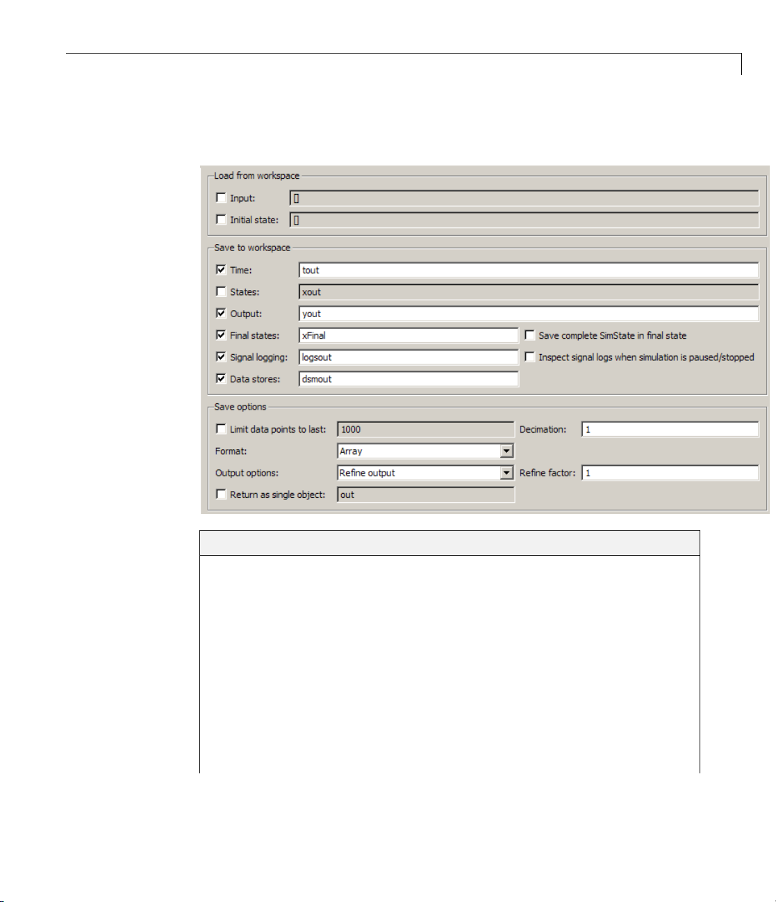
Data Import/Exp

The Data Import/ state data from a MATLAB standard or cus signals and to

Export pane allows you to import input signal and initial

workspace and export output signal and state data to the

worksp

tom MATLAB functions to generate a simulated system’s input

graph, analyze, or otherwise postprocess the system’s outputs.

ort Overview

ace during simulation. This capability allows you to use

Configuration

1 Specify the data to load from a workspace before simulation begins.

2 Specify the data to save to the MATLAB workspace after simulation

completes.

Tips

• For more i

Simulati

• See the do

availab

nformation on using this pane, see Importing and Exporting

on Data.

cumentation of the

leonlyforprogrammaticsimulation.

sim command for some cap a bilities th at are

Input

Loads input data from a workspace be fore the simulation beg ins.

Settings

Default: Off, [t,u]

Loads data from a workspace.

Specify a MATLAB expression for the data to be imported from a workspace. The Simulink software resolves symbols used in this specification as de scrib ed in “Resolving Symbols”. Th e input data can take any of the following forms:

• Time series

• Data array

• Time expression

1-80

• Data structure

See Importing Data from a Workspace for information on how to use this field.

Off

Does not load data from a workspace.

Tips

• You must select the Input check box before entering input data.

• Simulink software linearly interpolates or extrapolates input values as

necessary if the Interpolate data option is selected for the corresponding Inport.

• The use of the Input box is independent of the setting of the Format list

on the Data Import/Export pane.

Command-Line Information

Parameter: LoadExternalInput Type: string Value: Default: 'off'

Parameter: ExternalInput Type: scalar or vector Value: any valid value Default:

'on' | 'off'

[t,u]

Recommended Settings

Data Import/Export Pane

Application

Debugging No impact

Traceability No impact

Efficiency

Safety precaution No impact for simulation and during

Setting

No impact

development Off for production code generation

Initial state

Loads the model’

Settings

Default: Off,

Simulink software loads initial states from a workspace.

Specify the name of a variable that contains the initial state values, for example, a variable containing states saved from a previous simulation.

Use the structure or structure-with-time option to specify initial states if you want to accomplish any of the following:

• Associate initial state values directly with the full path name to the

states. This eliminates errors that could occur if Simulink software reorders the states, but the initial state array is not correspondingly reordered.

s initial states from a workspace before simulation begins.

xInitial

1-82

• Assign a different data type to each state’s initial value.

• Initialize only a subset of the states.

See Importing and Exporting States for more information.

Off

Simulink softw are does not load initial states from a workspace.

Tips

• You must select the Initial State check box before entering initial state

data.

• The initial values specified by the workspace variable override the initial

values specified by the model itself (thevaluesspecifiedbytheinitial condition parameters of those blocks in the model that have states).

• You must use the structure or structure-with-time format to initialize the

states of a top model and the models that it references.

Command-Line Information

Parameter: LoadInitialState Type: string Value: Default: 'off'

Parameter: InitialState Type: variable (string) or vector Value: any valid value Default:

'on' | 'off'

'xInitial'

Recommended Settings

Data Import/Export Pane

Application

Debugging No impact

Traceability No impact

Efficiency

Safety precaution No impact for simulation and during

Setting

No impact

development Off for production code generation

Time

Saves simulation time data to the specified v ariable during simulation.

Settings

Default: On, tout

Simulink software exports time data to the MATLAB workspace during simulation.

Specify the name of the MATLAB variable used to store time data. See Exporting Data to the MATLAB Works pace for more information.

Off

Simulink software does not export time data to the MATLAB workspace during simulation.

Tips

1-84

• You must

• Simulin

sample r output

• The Sav

amount

select the Time check box befo re entering the time variable.

ksoftwaresavestheoutputtotheMATLABworkspaceatthebase

ate of the model. Use a To Workspace block if you want to save

at a different sample rate.

eoptionsarea enables you to specify the format and restrict the

of output saved.

Command-Line Information

meter:

Para Type: string Value:

ult:

Defa

Parameter: TimeSaveName

e: string

Typ Value: any valid value Default:

SaveTime

'on' | 'off'

'on'

'tout'

Recommended Settings

Data Import/Export Pane

Application

Debugging No impact

Traceability No impact

Efficiency

Safety precaution No impact for simulation and during

Setting

No impact

development Off for production code generation

States

Saves state data

Settings

Default: Off,

Simulink software exports state data to the MATLAB w orkspace during simulation.

Specify the name of the MATLAB variable used to store state data. See Importing a nd Exporting States for more information.

Off

Simulink does not export state data during simulation.

Tips

to the specified MATLAB variable during a simulation.

xout

1-86

• You must select the States check box before entering the states variable.

• Simulink saves the states in a MATLAB workspace variable having the

specified name.

• The saved data has the format that you specify in the Save options area.

• Simulink creates empty variables for state logging (

conditions apply:

xout)ifbothofthese

- You enable States.

- A model has no states.

Command-Line Information

Parameter: SaveState Type: string Value: Default: 'off'

Parameter: StateSaveName Type: string Value: any valid value Default:

'on' | 'off'

'xout'

Recommended Settings

Data Import/Export Pane

Application

Debugging No impact

Traceability No impact

Efficiency

Safety precaution No impact for simulation and during

Setting

No impact

development Off for production code generation

Output

Saves signal data to the specified MATLAB variable during simulation.

Settings

Default: On, yout

Simulink software exports signal data to the MATLAB workspace during simulation.

SpecifythenameoftheMATLABvariableusedtostoresignaldata. See Exporting Data to the MATLAB Works pace for more information.

Off

Simulink software does not export signal data during simulation.

Tips

1-88

• You must select the Output check box before entering the output variable.

• Simulink software saves the output to the MATLAB workspace at the base

sample rate of the m odel. Use a To Workspace block if you want to save output at a different sample rate.

• The Save options area enables you to specify the format and restrict the

amount of output saved.

Command-Line Information

Parameter: SaveOutput Type: string Value: Default: 'on'

Parameter: OutputSaveName Type: string Value: any valid value Default:

'on' | 'off'

'yout'

Recommended Settings

Data Import/Export Pane

Application

Debugging No impact

Traceability No impact

Efficiency

Safety precaution No impact for simulation and during

Setting

No impact

development Off for production code generation

Final states

Saves the logged MATLAB variable

Settings

Default: Off,

Simulink software exports final logged state data to the MATLAB workspace during simulation.

Specify the name of the MATLAB variable in which to store the values of these final states. Se e Importing and Exporting States for more information.

Off

Simulink software does not export the final state data during simulation.

states of the model at the end of a simulation to the specified

xFinal

1-90

Tips

• You must select the Final states check box before entering the final states

variable.

• Simulink software saves the final states in a MATLAB workspace variable

having the specified name.

• The saved data has the format that you specify in the Save options area.

• Simulink creates empty variables for final state logging (

these conditions apply:

xfinal)ifbothof

- You enable Final states.

- A model has no states.

Command-Line Information

Parameter: SaveFinalState Type: string Value: Default: 'off'

Parameter: FinalStateName Type: string Value: any valid value Default:

'on' | 'off'

'xFinal'

Recommended Settings

Data Import/Export Pane

Application

Debugging No impact

Traceability No impact

Efficiency

Safety precaution No impact for simulation and during

Setting

No impact

development Off for production code generation

Save complete SimState in final state

At the end of a simulation, Simulink saves the complete set of states of the model, including logged states, to the specified MATLAB variable.

Settings

Default: Off, xFinal

Simulink software exports the complete set of final state data (i.e., the SimState) to the MATLAB workspace during simulation.

Specify the name of the MATLAB variable in which to store the values of the final states. See Importing and Exporting States for more information.

Off

Simulink software exports the final logged states during simulation.

1-92

Tips

• You must select the Final states check b ox to enable the Save complete

SimState in final state option.

• Simulink saves the final states in a MATLAB workspace variable having

the specified name.

• The saved data has the format that you specify in the Save options area.

Dependencies

This parameter is enabled by Final states.

Command-Line Information

Parameter: SaveCompleteFinalSimState Type: string Value: Default: 'off'

Parameter: FinalStateName

'on' | 'off'

Type: string Value: any valid value Default:

'xFinal'

Recommended Settings

Data Import/Export Pane

Application

Debugging No impact

Traceability No impact

Efficiency

Safety precaution

Setting

No impact

Signal logging

Globally enable

Settings

Default: On, l

Enables signal logging to the MATLAB workspace during simulation.

Specify the name of the signal logging object used to record logged signal data in the MATLAB workspace. See Logging Signals for more information.

Off

Disables signal logging to the MATLAB workspace during simulation.

Tips

or disable signal logging for this model.

ogsout

Data Import/Export Pane

• You must select the Signal logging check box before entering the signal

logging variable.

• Simulink software saves the signal data in a MATLAB workspace variable

having the specified name.

• The saved data has the format that you specify in the Save options area.

• Simulink software does not support signal logging for the following types of

signals:

- Output of a Function-Call Generator block

- Signal connected to the input of a Merge block

- Outputs of Trigger and Enable blocks

Dependencies

This parameter enables Inspect signal logs when simulation is paused/stopped.

1-95

1 Configuration Parameters Dialog Box

Command-Line Information

Parameter: SignalLogging Type: string Value: Default: 'on'

Parameter: SignalLoggingName Type: string Value: any valid value Default:

Recommended Settings

'on' | 'off'

'logsout'

Application

Debugging No impact

Traceability No impact

Efficiency

Safety precaution No impact for simulation and during

Setting

No impact

development Off for production code generation

Mathworks SIMULINK 7 Graphical User Interface

Specifications and Main Features

Frequently Asked Questions

User Manual

Configuration Parameters Dialog Box

Configuration Parameters Dialog Box Overview

Model Configuration Pane

Model Configuration Overview

Name

Settings

Description

Settings

Solver Pane

Solver Overview

Configuration

Tips

Start time

Settings

Command-Line Information

Recommended Settings

See Also

Stop time

Settings

Command-Line Information

Recommended Settings

See Also

Type

Settings

Dependencies

Command-Line Information

Recommended Settings

See Also

Solver

Settings

Tips

Dependencies

Command-Line Information

Recommended Settings

See Also

Max Step Size

Settings

Tips

Dependencies

Command-Line Information

Recommended Settings

See Also

Settings

Tips

Dependencies

Command-Line Information

Recommended Settings

See Also

Min Step Size

Settings

Tips

Recommended Settings

See Also

Settings

Tips

Dependencies

Command-Line Information

Recommended Settings

See Also

Settings

end of the simulation the Absolute tolerance is set to 1e-3.

Tips

Dependencies

Command-Line Information

Recommended Settings

See Also

Maximum order

Settings

Tips

Dependencies

Command-Line Information

Recommended Settings

See Also

Settings

Tips

Dependencies