

Page 1

Simscape™ 3
Reference
Page 2
How to Contact The MathWorks
www.mathworks.
comp.soft-sys.matlab Newsgroup
www.mathworks.com/contact_TS.html T echnical Support
suggest@mathworks.com Product enhancement suggestions
bugs@mathwo
doc@mathworks.com Documentation error reports
service@mathworks.com Order status, license renewals, passcodes
info@mathwo
com
rks.com
rks.com
Web
Bug reports
Sales, prici
ng, and general information
508-647-7000 (Phone)
508-647-7001 (Fax)
The MathWorks, Inc.
3 Apple Hill Drive
Natick, MA 01760-2098
For contact information about worldwide offices, see the MathWorks Web site.
Simscape™ Reference
© COPYRIGHT 2007–20 10 by The MathWorks, Inc.
The software described in this document is furnished under a license agreement. The software may be used
or copied only under the terms of the license agreement. No part of this manual may be photocopied or
reproduced in any form without prior written consent from The MathW orks, Inc.
FEDERAL ACQUISITION: This provision applies to all acquisitions of the Program and Documentation
by, for, or through the federal government of the United States. By accepting delivery of the Program
or Documentation, the government hereby agrees that this software or documentation qualifies as
commercial computer software or commercial computer software documentation as such terms are used
or defined in FAR 12.212, DFARS Part 227.72, and DFARS 252.227-7014. Accordingly, the terms and
conditions of this Agreement and only those rights specified in this Agreement, shall pertain to and govern
theuse,modification,reproduction,release,performance,display,anddisclosureoftheProgramand
Documentation by the federal government (or other entity acquiring for or through the federal government)
and shall supersede any conflicting contractual terms or conditions. If this License fails to meet the
government’s needs or is inconsistent in any respect with federal procurement law, the government agrees
to return the Program and Docu mentation, unused, to The MathWorks, Inc.
Trademarks
MATLAB and Simulink are registered trademarks of The MathWorks, Inc. See
www.mathworks.com/trademarks for a list of additional trademarks. Other product or brand
names may be trademarks or registered trademarks of their respective holders.
Patents
The MathWorks products are protected by one or more U.S. patents. Please see
www.mathworks.com/patents for more information.
Page 3

Revision History
March 2007 Online only New for Version 1.0 (Release 2007a)
September 2007 Online only Revised for Version 2.0 (Release 2007b)
March 2008 Online only Revised for Version 2.1 (Release 2008a)
October 2008 Online only Revised for Version 3.0 (Release 2008b)
March 2009 Online only Revised for Version 3.1 (Release 2009a)
September 2009 Online only Revised for Version 3.2 (Release 2009b)
March 2010 Online only Revised for Version 3.3 (Release 2010a)
Page 4

Page 5

Block Reference
1
Foundation ....................................... 1-2
Electrical
Hydraulic
Magnetic
Mechanical
Physical Signals
Pneumatic
Thermal
........................................ 1-2
........................................ 1-5
........................................ 1-6
....................................... 1-7
.................................. 1-10
....................................... 1-12
......................................... 1-14
Contents
Utilities
........................................... 1-16
v
Page 6

Blocks — Alphabetical List
2
Function Reference
3
Language Reference
4
Simscape Foundation Domains
5
Domain Types and Directory Structure .............. 5-2
vi Contents
Electrical Domain
Hydraulic Domain
Magnetic Dom ain
Mechanical Rotational Domain
Mechanical Translational Domain
Pneumatic Domain
Thermal Domain
................................. 5-4
................................. 5-5
.................................. 5-7
................................ 5-10
.................................. 5-12
..................... 5-8
.................. 5-9
Page 7

Configuration Parameters
6
Simscape Pane: General ............................ 6-2
Simscape Pane Overview
Editing Mode
Explicit solver used in model containing Physical Networks
blocks
Input f il teri ng used in model containing Physical Networks
blocks
Log simulation data
Workspace v aria ble name
Limit data points
Data history (last N steps)
..................................... 6-5
......................................... 6-7
......................................... 6-9
.................................. 6-12
........................... 6-4
............................... 6-10
........................... 6-11
.......................... 6-13
Bibliography
A
Glossary
Index
vii
Page 8

viii Contents
Page 9

Block Reference
1
Foundation (p. 1-2 )
Utilities (p. 1-16) Essential environment blocks for
Basic hydraulic, pneumatic,
mechanical, electrical, magnetic,
thermal, and physical signal blocks
creating Physical Networks models
Page 10

1 Block Reference
Foundation
Electrical (p. 1-2)
Hydraulic (p. 1-5)
Magnetic (p.
Mechanical (p. 1-7) Mechanical elements for rotational
Physical Signals (p. 1-10) Blocks for transmitting physical
Pneumatic (p. 1-12)
Thermal (p. 1-14)
1-6)
Basic electrical diagram blocks, such
as inductors, diodes, capacitors,
sensors and source s
Basic hydraul
such as orif ic
and sources,
Basic electromagnetic diagram
blocks, such as reluctances,
electromagnetic converters, sensors
and sources
and translational motion, as well as
mechanical sensors and sources
control signals
Basic pneumatic diagram blocks,
such as orifices, chambers, sensors
and s ou rces, and pneumatic utilities
thermal blocks, such as heat
Basic
sfer blocks, thermal mass,
tran
ors and source s
sens
ic diagram blocks,
es, chambers, sensors
and hydraulic utilities
1-2
Electrical
ctrical E lements (p. 1-3)
Ele
Electrical Sensors (p. 1-4) Current and voltage sensors
Electrical Sources (p. 1-4) Current and voltage sources
Electrical building blocks, such as
inductors, diodes, and capacitors
Page 11

Electrical Elements
Capacitor Simulate linear capacitor in
electrical systems
Foundation
Diode
Electrical Reference Simulate connection to electrical
Gyrator Simulate ideal gyrator in electrical
Ideal Transformer Simulate ideal transformer in
Inductor
Mutual Inductor
Op-Amp Simulate ideal operational amplifier
Resistor
Rotational Electromechanical
Converter
Switch Simulate switch controlled by
Translational Electromechanical
Converter
Simulate piecewise linear diode in
electrical systems
ground
systems
electrical systems
Simulate linear inductor in electrical
systems
Simulate mutual inductor in
electrical systems
Simulate linear resistor in electrical
systems
Provide i nterface between electrical
and mechanical rotational domains
external physical signal
Provide i nterface between electrical
and mechanical translational
domains
Variable Resistor
Simulate linear variable resistor in
electrical systems
1-3
Page 12

1 Block Reference
Electrical Sensors
Current Sensor Simulate current sensor in electrical
systems
Voltage Sensor Simulate v oltage sensor in electrical
systems
Electrical Sources
AC Current Source Simulate ideal sinusoidal current
source
AC Voltage Source Simulate ideal constant voltage
source
Controlled Current Source Simulate ideal current source driven
by input signal
Controlled Voltage Source Simulate ideal voltage source driven
by input signal
1-4
Current-Controlled Current Source Simulate linear current-controlled
current source
Current-Controlled Voltage Source Simulate linear current-controlled
voltage source
DC Current Source Simulate ideal constant current
source
DC Voltage Source Simulate ideal constant voltage
source
Voltage-Controlled Current Source Simulate linear voltage-controlled
current source
Voltage-Controlled Voltage Source Simulate linear voltage-controlled
voltage source
Page 13

Hydraulic
Foundation
Hydraulic Elements (p. 1-5)
Hydraulic Sen
Hydraulic So
Hydraulic Ut
sors (p. 1-6)
urces (p. 1-6)
ilities (p. 1-6)
Hydraulic Elements
Constant A
Constant
Chamber
Fluid Inertia
Hydra
Hydr
rea Hydraulic Orifice
Volume Hydraulic
ulic Piston Chamber
aulic Reference
Hydraulic build
such as orifice
hydro-mechani
Hydraulic sensors
Hydraulic sources
Basic hydraulic environment blocks,
such as custom hydraulic fluid
Simulate h
constant
Simulate
constan
Simulat
tube or
fluid v
Simul
capac
Simu
pres
cross-sectional area
tvolume
e pressure differential across
channel due to change in
elocity
ate variable volume hydraulic
ity in cylind ers
late connection to atmospheric
sure
ing blocks,
s, chambers, and
cal converters
ydraulic orifice with
hydraulic capacity of
Hydraulic Resistive Tube
Linear Hydraulic Resistance
Rotational Hydro-Mechanical
Converter
Translational Hydro-Mechanical
Converter
late hydraulic pipeline which
Simu
ounts for friction losses only
acc
ulate hydraulic pipeline with
Sim
near resistance losses
li
mulate ideal hydro-mechanical
Si
ansducer as building block for
tr
otary actuators
r
imulate single chamber of hydraulic
S
cylinder as building block for various
cylinder models
1-5
Page 14

1 Block Reference
Variable Area Hydraulic O rifice Simulate hydraulic variable orifice
created by cylindrical spool and
sleeve
Variable Hydraulic Chamber Simulate hydraulic capacity of
variable volume with compressible
fluid
Hydraulic Sensors
Hydraulic Flow Rate Sensor Simulate ideal flow meter
Hydraulic Pressure Sensor Simulate ideal pressure sensing
device
Hydraulic Sources
Hydraulic Flow Rate Source Simulate ideal source of hydraulic
energy, characterized by flow rate
1-6
Hydraulic Pressure Source Simulate ideal source of hydraulic
energy, characterized by pressure
Hydraulic Utilities
Custom Hydraulic Fluid Set working fluid prop erties by
specifying parameter values
Magnetic
Magnetic Elements (p. 1-7)
Magnetic Sensors (p. 1-7) Flux and mmf sensors
Magnetic Sources (p. 1-7) Flux and mmf sources
Magnetic building blocks, such
as reluctances, electromagnetic
converters, and actuators
Page 15

Magnetic Elements
Electromagnetic Converter Simulate lossless electromagnetic
energy conversion device
Magnetic Reference Simulate reference for magnetic
ports
Foundation
Reluctance
Reluctance Force Actuator Simulate magnetomotive device
Variable R eluctance
Simulate magnetic reluctance
based on reluctance force
Simulate variable reluctance
Magnetic Sensors
Flux Sensor Simulate ideal flux s ensor
MMF Sensor Simulate ideal magnetomotive force
sensor
Magnetic Sources
Controlled Flux Source Simulate ideal flux source driven by
input signal
Controlled MMF Source Simulate ideal magnetomotive force
source driven by input signal
Flux Source Simulate ideal flux source
MMF Source Simulate ideal magnetomotive force
source
Mechanical
Mechanical Sensors (p. 1-8)
Mechanical Sources (p. 1-8)
Mechanisms (p. 1-9)
Mechanical sensors and sources
Mechanical sensors and sources
Various simple mechanisms
1-7
Page 16

1 Block Reference
Rotational E lements (p. 1-9) Mechanical elements for rotational
motion
Translational Elements (p. 1-9) Mechanical elements for
translational motion
Mechanical Sensors
Ideal Force Sensor Simulate force sensor in mechanical
translational systems
Ideal Rotational Motion Sensor Simulate motion sensor in
mechanical rotational systems
Ideal Torque Sensor Simulate torque sensor in
mechanical rotational systems
Ideal Trans lational Motion Sensor Simulate motion sensor in
mechanical translational systems
1-8
Mechanical Sources
Ideal Angular Velocity Source Simulate ideal angular velocity
source in mechanical rotational
systems
Ideal Force Source Simulate ideal source of mechanical
energy that generates force
proportional to the input signal
Ideal Torque Source Simulate ideal source of mechanical
energy that generates torque
proportional to the input signal
Ideal Translational Velocity Source Simulate ideal velocity source in
mechanical translational systems
Page 17

Mechanisms
Gear Box Simulate gear bo xe s in mechanical
systems
Foundation
Lever
Wheel and Axle Simulate wheel and axle mechanism
Simulate lever in mechanical
systems
in mechanical system s
Rotational Elements
Inertia
Mechanical Rotational Reference Simulate reference for mechanical
Rotational Damper
Rotational Friction
Rotational Hard Stop Simulate double-sided rotational
Rotational Spring Simulate ideal spring in mechanical
Simulate inertia in mechanical
rotational systems
rotational ports
Simulate viscous damper in
mechanical rotational systems
Simulate friction in contact between
rotating bodies
hard stop
rotational systems
Translational Elements
Mass
Mechanical Translational Reference Simulate reference for mechanical
Translational Damper
Simulate mass in mechanical
translational systems
translational ports
Simulate viscous damper in
mechanical translational systems
1-9
Page 18

1 Block Reference
Translational Friction
Translational Hard Stop Simulate double-sided translational
Translational Spring Simulate ideal spring in mechanical
Simulate friction in contact between
moving bodies
hard stop
translational systems
Physical Signals
Functions (p. 1-10) Perform math operations on physical
signals
Linear Operators (p. 1-11) Simulate continuous-time functions
for physical signals
Lookup Tables (p. 1-11) Perform one- and two-dimensional
table lookup to generate physical
signals
Nonlinear O perators (p. 1-11) Simulate discontinuities, such as
saturation or dead zone, for physical
signals
Sources (p. 1-12) Simulate physical signal sources
1-10
Functions
PS Add Add two physical signal inputs
PSDivide Computesimpledivisionoftwo
input physical signals
PS Gain
PS Math Function Apply mathematical function to
Multiply input physical signal by
constant
input physical signal
Page 19

Foundation
PS Product
PS Subtract Compute simple subtraction of two
Multiply two physical signal inputs
input physical signals
Linear Operators
PS Integrator
Integrate physical signal
Lookup Tables
PS Lookup Table (1D) Approximate one-dimensional
function using specified lookup
method
PS Lookup Table (2D) Approximate two-dimensional
function using specified lookup
method
Nonlinear Operators
PS Abs Output absolute value of input
physical signal
PS Ceil Output the smallest integer larger
than or equal to input physical signal
PS Dead Zone Provide region of zero output for
physical signals
PS Fix
PS Floor Output the largest integer smaller
PS Max Output maximum of two input
PS Min Output minimum of two input
Round input physical signal toward
zero
than or equal to input physical signal
physical signals
physical signals
1-11
Page 20

1 Block Reference
PS Saturation Limit range of physical signal
PS Sign Output sign of input physical signal
PS Switch Simulate single-pole double-throw
switch controlled by external
physical signal
Sources
PS Constant Generate constant physical signal
Pneumatic
Pneumatic Elements (p. 1-12)
Pneumatic Sensors (p. 1-13)
Pneumatic Sources (p. 1-13)
Pneumatic Utilities (p. 1-14)
Pneumatic building blocks,
such as orifices, chambers, and
pneumo-mechanical converters
Pneumatic sensors
Pneumatic sources
Basic pneumatic environment
blocks, s uch as gas properties
Pneumatic Elements
Adiabatic Cup Simulate thermal element with no
thermal mass and perfect insulation
Constant Area Pneumatic Orifice Simulate sharp-edged orifice in
pneumatic systems
Constant Area Pneumatic Orifice
(ISO 6358)
Constant Volume Pneumatic
Chamber
Simulate fixed-area pn eumatic
orifice complying with ISO 6358
standard
Simulate constant volume pneumatic
chamber based on ideal gas law
1-12
Page 21

Pneumatic A bso lute Reference Simulate reference to zero absolute
pressure and temperature for
pneumatic ports
Pneumatic Atmospheric Reference Simulate reference to ambient
pressure and temperature for
pneumatic ports
Pneumatic Piston Chamber Simulate translational pneumatic
piston chamber based on ideal gas
law
Foundation
Pneumatic Resistive Tube
Rotary Pneumatic Piston Chamber Simulate rotational pneumatic
Rotational Pneumatic-Mechanical
Converter
Variable Area Pneumatic Orifice Simulate variable orifice in
Simulate pressure loss and added
heatduetoflowresistancein
pneumatic pipe
piston chamber based on ideal gas
law
Provide interface between pneumatic
and mechanical rotational domains
pneumatic systems
Pneumatic Sensors
Pneumatic Mass & H eat Flow Sensor Simulate ideal mass flow and heat
flow sensor
Pneumatic Pressure & Temperature
Sensor
Simulate ideal pressure and
temperature sensor
Pneumatic Sources
Controlled Pneumatic Flow Rate
Source
Simulate ideal compressor with
signal-controlled mass flow rate
Controlled Pneumatic Pressure
Source
Simulate ideal compressor with
signal-controlled pressure difference
1-13
Page 22

1 Block Reference
Pneumatic Flow Rate Source Simulate ideal compressor with
constant mass flow rate
Pneumatic Pressure Source Simulate ideal compressor with
constant pressure difference
Pneumatic Utilities
Gas Properties Specify pneumatic domain properties
for attached circuit
Thermal
Thermal Elements (p. 1-14)
Thermal Sensors (p. 1-15) Temperature and heat flow sensors
Thermal Sources (p. 1-15) Temperature and heat flow sensors
Thermal building blocks, such as
thermal mass and various heat
transfer blocks
and sources
and sources
Thermal Elements
Conductive Heat Transfer Simulate heat transfer by conduction
Convective Heat Transfer Simulate heat transfer by convection
Radiative Heat Transfer Simulate heat transfer by radiation
Thermal Mass
Thermal Reference Simulate reference for thermal ports
Simulate mass in thermal systems
1-14
Page 23

Thermal Sensors
Ideal Heat Flow Sensor Simulate ideal heat flow meter
Ideal Temperature Sensor Simulate ideal temperature sensor
Thermal Sources
Ideal Heat Flow Source Simulate ideal source of thermal
energy, characterized by heat flow
Ideal Temperature Source Simulate ideal source of
thermal energy, characterized
by temperature
Foundation
1-15
Page 24

1 Block Reference
Utilities
Connection Port Create P hysical Modeling connector
port for subsystem
PS-Simulink Converter Convert physical signal into
Simulink
Simulink-PS Converter Convert Simulink input signal into
physical signal
Solver Configuration
Two-Way Connection Create two-way connector port for
Represent Physical Networks
environment and solver
configuration
subsystem
®
output signal
1-16
Page 25

2
Blocks — Alphabetical List
Page 26

AC Current Source
Purpose Simulate ide al sinusoidal current source
Library Electrical Sources
Description The AC Current Source block represents an ideal current source that
maintains sinusoidal current through it, independent of the voltage
across its terminals.
The output current is defined by the following equation:
II t=+
iisin( )ωϕ
0
where
Dialog
Box a nd
Parameters
I
I
0
ω
φ
t
The p ositive direction of the current flow is indicated by the arro w.
Current
Peak amplitude
Frequency
Phase shift
Time
2-2
Page 27

AC Current Source
Peak amplitude
Peak current amplitude. The default value is 10*sqrt(2), or
14.1421 A.
Phase shift
Phase shift in angular units. The default value is
Frequency
Current frequency. The default value is
60 Hz.
Ports The block has two electrical conserving ports associated with its
terminals.
See Also AC Voltage Source
0.
2-3
Page 28

AC Voltage Source
Purpose Simulate ideal constant voltage source
Library Electrical Sources
Description The AC Voltage Source block represents an ideal voltage source that
maintains sinusoidal voltage across its output terminals, independent
of the current flowing through the source.
The output voltage is defined by the following equation:
VV t=+
where
V
V
0
ω
φ
t
Connections + and – are conserving electrical ports corresponding to the
positive and negative terminals of the voltage source, respectively. The
current is positive if it flows from positive to negative, and the voltage
across the source is equal to the difference between the voltage at the
positive and the negative terminal, V(+) – V(–).
iisin( )ωϕ
0
Voltage
Peak amplitude
Frequency
Phase shift
Time
2-4
Page 29

Dialog
Box a nd
Parameters
AC Voltage Source
Peak amplit
Peak voltag
169.71 V.
Phase shif
Phase shi
Frequenc
Voltage f
ude
e amplitude. The default value is 120*sqrt(2), or
t
ft in angular units. The default value is
y
requency. The default value is
Ports The block has the following ports:
+
Electrical conserving port associated with the source positive
terminal.
Electrical conserving port associated with the source negative
terminal.
See Also AC Current Source
0.
60 Hz.
2-5
Page 30

Adiabatic Cup
Purpose Simulate thermal element with no thermal mass and perfect insulation
Library Pneumatic Elements
Description The Adiabatic Cup block models a thermal element w ith no thermal
mass and perfect insulation. Use this block as an insulation for thermal
ports to prevent heat exchange with the environment and to model
an adiabatic process.
Dialog
Box a nd
Parameters
The block has no parameters.
Ports The block has one pneumatic conserving port.
2-6
Page 31

Capacitor
Purpose Simulate linear capacitor in electrical systems
Library Electrical Elements
Description The Capacitor block models a linear capacitor, described with the
following equation:
dV
IC
=
dt
where
I
V
C
t
The Initial voltage parameter sets the initial voltage across the
capacitor.
Note This value is not used if the solver configuration is set to Start
simulation from steady state.
The Series resistance and Parallel conductance parameters
represent small parasitic effects. The parallel conductance directly
across the capacitor can be used to model dielectric losses, or
equivalently leakage current per volt. The series resistance can be used
to represent component effective series resistance (ESR) or connection
resistance. Simulation of some circuits may require the presence of
the small series resistance. For more information, see “Modeling Best
Practices” in the Simscape™ User’s Guide.
Connections + and – are conserving electrical ports corresponding to
the p ositive and negative terminals of the capacitor, respectively. The
Current
Voltage
Capacitance
Time
2-7
Page 32

Capacitor
Dialog
Box a nd
Parameters
current is positive if it flows from positive to negative, and the voltage
across the capacitor is equal to the difference betw een the voltage at the
positive and the negative terminal, V(+) – V(–).
2-8
Capacitance
Capacitance, in farads. The default value is
Initial voltage
Initial voltage across the capacitor. This parameter is not used if
the solver configuration is set to Start simulation from steady
state. The default value is
Series resistance
Represents small parasitic effects. The series resistance can be
used to represent component internal resistance. Simulation
of some circuits may require the presence of the small series
resistance. The default value is
0.
1 µΩ.
1 µF.
Page 33

Parallel conductance
Represents small parasitic effects. The parallel conductance
directly across the capacitor canbeusedtomodelleakagecurrent
per volt. The default value is
Ports The block has the following ports:
+
Electrical conserving port associated with the capacitor positive
terminal.
-
Electrical conserving port as sociated with the capacitor negative
terminal.
Capacitor
0.
2-9
Page 34

Conductive Heat Transfer
Purpose Simulate heat transfer by conduction
Library Thermal Elements
Description The Conductive Heat Transfer block represents a heat transfer by
conduction between two layers of thesamematerial. Thetransfer
is governed by the Fourier law and is described with the following
equation:
A
Qk
=−i ()
where
Q Heat flow
k Material thermal conductivity
TT
AB
D
A
D
T
A,TB
Connections A and B are thermal conserving ports associated with
material layers. The block positive direction is from port A to port B.
This means that the heat flow is positive if it flows from A to B.
Area normal to the h eat flow direction
Distance between layers
Temperatures of the layers
2-10
Page 35

Dialog
Box a nd
Parameters
Conductive Heat Transfer
Area
Area of heat transfer, normal to the heat flow direction. The
default value is
Thickness
Thickness between layers. The default value is
0.0001 m^2.
0.1 m.
Thermal conductivity
Thermal conductivity of the material. The default value is
W/m/K.
Ports The block has the following ports:
A
Thermal conserving port associated with layer A.
B
Thermal conserving port associated with layer B.
See Also Convective Heat Transfer
Radiative Heat Transfer
401
2-11
Page 36

Connection Port
Purpose Create Physical Modeling connector port for subsystem
Library Utilities
Description The Connection Port block transfers both the conserving and the
physical signal connections to the outside boundary of a subsystem
block. This transfer is similar to the Inport and Outport blocks in
Simulink models. A subsystem needs a Connection Port block for each
physical connection line that crosses its boundary. You can manually
place a Conne ction Port block inside a subsystem, or Simulink can
automatically insert a Connection P ort block when you create a
subsystemwithinanexistingnetwork.
Port Appearance on Subsystem Boundary
The ports on the subsystem boundary change their appearance
depending on the type of port to which the Connection Port block is
connected inside the subsystem.
Connection Port Block Inside a
Subsystem Connects to ...
A Conserving port
A Physical Signal inport or outport
Atwo-wayconnectorportofthe
Two-Way Connection block
A SimMechanics™ connector port,
either:
Round connector port Round connector port
Body coordinate sys tem
port
2-12
... and Appears on the Outside Boundary of
the Subsystem as ...
A square Conserving port
A triangular Physical Signal
A two-way connector port
A SimMechanics connector port, either:
Body coordinate system port
inport or outport
Page 37

Connection Port
Port Location and Orientation on Subsystem Boundary
The orientation of the parent subsystem block and your choice of port
location determine the Connection Port block port location on the p arent
subsystem boundary.
• A subsystem is in its fundamental orientation when its Simulink
signal inports occur on its left side and its Simulink signal outports
occur on its right side.
When a subsystem is oriented in this way, the actual port location
on the subsystem boundary respects your choice of port location (left
or right) for the connector port.
• A subsyste m orientation is reversed, with left and right interchanged,
when its Simulink signal inports occur on i ts right side and its
Simulink signal outports occur on its left side.
When a subsystem is oriented in this way, the actual port location on
the subsystem boundary reverses your choice of port location. If you
choose left, the port appears on the right side. If you choose right,
the port appears on the left side.
2-13
Page 38

Connection Port
Dialog
Box a nd
Parameters
Port number
Labels the subsystem connector port that this block creates. Each
connector port on the boundary of a single subsystem requires a
unique number as a label. The default v alue for the first port is
1.
Port location on parent subsystem
Choose here which side of the parent subsystem boundary the
port is located. T h e choices are
is
Left.
See “Port Location and Orientation on Subsystem Boundary” on
page 2-13.
Left or Right. The default choice
See Also In the Simulink User’s Guide, see “Working w ith Block Masks”.
2-14
Page 39

Constant Area Hydraulic Orifice
⎝
⎠
Purpose Simulate hydraulic orifice with constant cross-sectional area
Library Hydraulic Elements
Description The Constant Area Hydraulic Orifice block models a sharp- e d ged
constant-area orifice. T he model distinguishes between the laminar and
turbulent flow regimes by comparing the Reynolds number with its
critical value. The flow rate through the orifice is proportional to the
pressure differential across the orifice, and is determined according
to the follow i ng equations:
⎧
⎪
⎪
q
=
⎨
⎪
⎪
⎩
pp p
=−
Re =
C
DL
D
=
H
where
q
p
pA,p
B
C A p sign p Re Re
D
CADpReRe
2
AB
qD
i
A
⎛
=
⎜
⎜
| | for >=
ρ
H
i
DL
i
νρ
H
()
iν
2
⎞
C
D
⎟
⎟
Re
cr
A
4
for <
cr
cr
2
ii
π
Flow rate
Pressure differential
Gauge pressures at the block terminals
2-15
Page 40

Constant Area Hydraulic Orifice
Basic
Assumptions
and
Limitations
C
A
D
ρ
ν
Re
Re
D
H
Flow discharge coe fficient
Orifice passage area
Orifice hydraulic diameter
Fluid density
Fluid kinematic viscosity
Reynolds number
Critical Reynolds num ber
cr
The block positive direction is from port A to port B. This means
thattheflowrateispositiveifitflowsfromAtoB,andthepressure
differential is determined as
pp p
=−
AB
.
The model is based on the following assumptions:
• Fluid inertia is not taken into account.
• The transition between laminar and turbulent regimes is assumed to
be sharp and taking place exactly at
Re=Re
.
cr
2-16
Page 41

Dialog
Box a nd
Parameters
Constant Area Hydraulic Orifice
Orifice area
Orifice passage area. The default value is
Flow discharge coefficient
Semi-empirical parameter for orifice capacity characterization.
Its value depends on the geometrical properties of the orifice, and
usually is provided in textbooks or manufacturer data sheets.
The default value is
Critical Reynolds number
The maximum Reynolds number for laminar flow. The transition
from laminar to turbulent re gime is supposed to take place
when the Reynolds number reaches this value. The value
of the parameter depends on orifice geometrical profile, and
the recommendations on the parameter value can be found in
hydraulic textbooks. The default value is
a round orifice in thin material with sharp edges.
0.7.
1e-4 m^2.
12, which corresponds to
2-17
Page 42

Constant Area Hydraulic Orifice
Global
Parameters
Fluid density
The parameter is determined by the type of working fluid selected
for the system under design. Use the Custom Hydraulic Fluid
block, or the Hydraulic Fluid block a vailable with SimHydraulics
block libraries, to specify the fluid properties.
Fluid kinematic viscosity
The parameter is determined by the type of working fluid selected
for the system under design. Use the Custom Hydraulic Fluid
block, or the Hydraulic Flui d block available with SimHydraulics
block libraries, to specify the fluid properties.
Ports The block has the following ports:
A
Hydraulic co n serving port a sso ciated with the orifice inlet.
B
Hydraulic conserving port associated with the orifice outlet.
See Also Variable Area Hydraulic Orifice
®
2-18
Page 43

Constant Area Pneumatic Orifice
Purpose Simulate sharp-edged orifice in pneumatic systems
Library Pneumatic Elements
Description The Constant Area Pneumatic Orifice block models the flow rate of an
ideal gas through a sharp-edged orifice.
Theflowratethroughtheorificeisproportion al to the orifice area and
the pressure differential across the orifice.
+
γ
⎤
γ
⎞
⎛
p
⎜
p
⎝
⎥
o
⎟
⎥
i
⎠
⎥
⎦
GCAp
=
ii i
di
γ
211
γ
−
⎡
⎛
⎢
⎜
⎢
RTpp
i
⎝
⎢
⎣
21
γ
⎞
o
−
⎟
i
⎠
where
G Mass flow rate
C
d
Discharge coefficient, to account for effective loss of area due
to orifice shape
A
p
i,po
Orifice cross-sectional area
Absolute pressures at the orifice inlet and outlet, respectively.
The inlet and outlet change depending on flow direction. For
positive flow (G >0),p
γ
R
T
The ratio of specific heats a t constant pressure and constant
volume, c
p/cv
Specific gas constant
Absolute gas temperature
= pA,otherwisepi= pB.
i
The choked flow occurs at the critical pressure ratio defined by
γ
β
==
cr
p
⎛
o
⎜
p
⎝
i
γ
−
1
⎞
2
⎟
1
γ
+
⎠
2-19
Page 44

Constant Area Pneumatic Orifice
after which the flow rate depends on the inlet pressure only and is
computed with the expression
+
γγ1
GCAp
=
ii i
diicr
The square root relationship has infinite gradient at zero flow, which
can present numerical solver difficulties. Therefore,forverysmall
pressure differences, defined by p
replaced by a linear flow-pressure relationship
GkCAT p p
=−
ii
di io
where k is a constant such that the flow predicted for po/piis the same
as that predicted by the original flow equatio n for p
Theheatflowoutoftheorificeisassumedequaltotheheatflowinto
the orifice, based on the following considerations:
γ
β
RT
−
05.
()
> 0.999, the flow equation is
o/pi
o/pi
=0.999.
2-20
• The orifice is square-edged or sharp-edged, and as such is
characterized by an abrupt change of the downstream area. This
means that practically all the dynamic pressure is lost in the
expansion.
• The lost energy appears in the form of internal energy that rises the
output temperature and makes it very close to the inlet temperature.
Therefore, q
= qo,whereqiand qoare the input and output heat flows,
i
respectively.
The block positive direction is from port A to port B. This means that
theflowrateispositiveifitflowsfromAtoB.
Page 45

Constant Area Pneumatic Orifice
Basic
Assumptions
and
Limitations
Dialog
Box a nd
Parameters
The model is based on the following assumptions:
• The gas is ideal.
• Specific heats at constant pressure and constant volume, c
are constant.
• The process is adiabatic, that is, there is no heat transfer with the
environment.
• Gravitational effects can be neglected.
• The orifice adds no net heat to the flow.
and cv,
p
Discha
Orifi
rge coefficient, Cd
Semi-e
Its val
usual
The de
ce area
Spec
m^2.
mpirical parameter for orifice capacity characterization.
ue depends on the geometrical properties of the orifice, and
ly is provided in textbooks or manufacturer data sheets.
fault value is
ify the orifice cross-sectional area. The default value is
0.82.
Ports The block has the following ports:
1e-5
2-21
Page 46

Constant Area Pneumatic Orifice
A
Pneumatic conserving port associated with the orifice inlet for
positive flow.
B
Pneumatic conserving port associated with the orifice outlet for
positive flow.
See Also Constant Area Pneumatic Orifice (ISO 6358)
Variable Area Pneumatic Orifice
2-22
Page 47

Constant Area Pneumatic Orifice (ISO 6358)
Purpose Simulate fixed-area pneumatic orifice complying with ISO 6358
standard
Library Pneumatic Elements
Description The Constant Area Pneumatic Orifice (ISO 6358) block models the flow
rate of an ideal gas through a fixed-area sharp-edged o rifice. The model
conforms to the ISO 6358 standard and is based on the following flow
equations, originally proposed by Sanville [1]:
⎧
kp
⎪
1
⎪
⎛
⎜
i
⎝
⎞
p
o
−
1iiif (laminarβ ))
⎟
p
i
⎠
⎪
⎪
⎪
⎪
G
=
ii iρβ1
⎨
i ref
⎪
T
ref
T
i
⎪
⎪
ii
T
ref
T
i
ρ
ref
⎪
iiρ<=
⎪
i ref
⎪⎪
⎩
1
=
kC
1
1
−
β
lam
where
G Mass flow rate
β
lam
Pressure ratio at laminar flow, a value between 0.999 and
0.995
b
Critical pressure ratio, that is, the ratio between the outlet
pressure p
and inlet pressure piat which the gas velocity
o
achieves sonic speed
T
ref
T
i
−
⎛
1
−
⎜
⎝
sign p p
⎛
⎜
⎜
⎜
⎜
⎝
β
lam
1
−
()
io
p
p
1
2
⎞
o
b
−
⎟
i
⎟
b
−
⎟
⎟
⎠
2
−
b
⎞
⎟
−
b
⎠
p
o
>
lam
p
i
p
o
if (pC
if (choked)pC
>>
lam
p
o
p
i
ssubsonic)
b
p
i
b
2-23
Page 48

Constant Area Pneumatic Orifice (ISO 6358)
C Sonic conductance of the component, that is, the ratio
between the mass flow rate and the product of inlet pressure
p
and the mass density at standard conditions when the flow
1
is choked
ρ
p
T
ref
i,po
i,To
Gas de nsity at standard conditions (1.185 kg/m^3 for air)
Absolute pressures at the orifice inlet and outlet, respectively.
The inlet and outlet change depending on flow direction. For
positive flow (G >0),p
= pA,otherwisepi= pB.
i
Absolute gas temperatures at the orifice inlet and outlet,
respectively
T
ref
Gas temperature at standard conditions (T
=293.15K)
ref
The equation itself, parameters b and C, and the heuristic on how
to measure these parameters experimentally form the basis for the
standard ISO 6358 (1989). The values of the critical pressure ratio
b and the sonic conductance C depend on a particular design of a
component. Typically, they are determined experimentally and are
sometimes given on a manufacturer data sheet.
The block can also be parameterized in terms of orifice effective area
or flow coefficient, instead of sonic conductance. When doing so,
block parameters are co nv erted into an equivalent value for sonic
conductance. When specifying effective area, the following formula
proposed by Gidlund and de tailed in [2] is used:
C =0.128d
2
where
C Sonic conductance in dm^3/(s*bar)
d
Inner diameter of restriction in mm
The effective area (whether specified directly, or calculated when the
orifice is parameterized in terms of C
or Kv, as described below) is used
v
2-24
Page 49

Constant Area Pneumatic Orifice (ISO 6358)
to determine the inner diameter d in the Gidlund formula, assuming a
circular cross section.
Gidlund also gives an approximate formula for the critical pressure
ratio in terms of the pneumatic line diameter D,
b = 0.41 + 0.272 d / D
This equation is not used by the block and you must specify the critical
pressure ratio directly.
If the orifice is parameterized in terms of the C
the C
coefficient is turned into an equivalent effective o rifice area for
v
[2] coefficient, then
v
use in the Gidlund formula:
A = 1.6986e – 5 C
v
By definition, an opening or restriction has a Cvcoefficient of 1 if it
passes 1 gpm (gallon per minute) of water at pressure drop of 1 psi.
If the orifice is parameterized in ter ms of the K
the K
coefficient is turned into an equivalent effective o rifice area for
v
[2] coefficient, then
v
use in the Gidlund formula:
A = 1.1785e – 6 C
Kvis the SI counterpart of Cv. An opening or restriction has a K
v
v
coefficient of 1 if it passes 1 lpm (liter per minute) of water at pressure
drop of 1 bar.
Theheatflowoutoftheorificeisassumedequaltotheheatflowinto
the orifice, based on the following considerations:
• The orifice is square-edged or sharp-edged, and as such is
characterized by an abrupt change of the downstream area. This
means that practically all the dynamic pressure is lost in the
expansion.
2-25
Page 50

Constant Area Pneumatic Orifice (ISO 6358)
• The lost energy appears in the form of internal energy that rises the
output temperature and makes it very close to the inlet temperature.
Basic
Assumptions
and
Limitations
Therefore, q
respectively.
The block positive direction is from port A to port B. This means that
theflowrateispositiveifitflowsfromAtoB.
The model is based on the following assumptions:
• The gas is ideal.
• Specific heats at constant pressure and constant volume, c
are constant.
• The process is adiabatic, that is, there is no heat transfer with the
environment.
• Gravitational effects can be neglected.
• The orifice adds no net heat to the flow.
= qo,whereqiand qoare the input and output heat flows,
i
and cv,
p
2-26
Page 51

Dialog
Box a nd
Parameters
Constant Area Pneumatic Orifice (ISO 6358)
2-27
Page 52

Constant Area Pneumatic Orifice (ISO 6358)
2-28
Orifice is s pecified with
Select one of the following model parameterization methods:
Page 53

Constant Area Pneumatic Orifice (ISO 6358)
• Sonic conductance —Providevalueforthesonicconductance
of the orifice. The values of the sonic conductance and the
critical pressure ratio form the basis for the ISO 6358 compliant
flow equations for the orifice. This is the default m ethod.
•
Effective area — Provide value for the orifice effective
area. This value is internally converted by the block into an
equivalent value for sonic conductance.
•
Cv coefficient (USCU) —Providevaluefortheflow
coefficient specified in US units. This value is internally
converted by the block into an equivalent value for the orifice
effective area.
•
Kv coefficient (SI) — Provide value for the flow coefficient
specified in SI units. This value is internally converted by the
block into an equivalent value for the orifice effective area.
Sonic conductance
Specify the sonic conductance of the orifice, that is, the ratio
between the mass flow rate and the product of upstream pressure
and the mass density at standard conditions w hen the flow is
choked. This value depends on the geometrical properties of the
orifice, and usually is provided in textbooks or manufacturer data
sheets. The default value is
in the dialog box if Orifice is specified with parameter is set
to
Sonic conductance.
1.6 l/s/bar. This parameter appears
Effective area
Specify the orifice cross-sectional area. The default value is
m^2. This parameter appears in the dialog box if Orifice is
specified with parameter is set to
Effective area.
Cv coefficient
Specify the value for the flow coefficient in US units. The default
value is
is specified with parameter is set to
0.6. This parameter appears in the dialog box if Orifice
Cv coefficient (USCU).
1e-5
2-29
Page 54

Constant Area Pneumatic Orifice (ISO 6358)
Kv coefficient
Specify the value for the flow coefficient in SI units. The default
value is
is specified with parameter is set to
Critical pressure ratio
Specify the critical pressure ratio, that is, the ratio between the
downstream pressure and the upstream pressure at w hich the gas
velocity achieves sonic speed. The default value is
Pressure ratio at laminar flow
Specify the ratio b etween the downstream pressure and the
upstream pressure at laminar flow. This value can be in the range
between 0.995 and 0.999. The default value is
Temperature at standard conditions
Specify the gas temperature at which the sonic conductance was
measured. The default value is
Pressure at standard conditions
Specify the gas pressure at which the sonic conductance was
measured. The default value is
8.5. This parameter appears in the dialog box if Orifice
Kv coefficient (SI).
293.15 K.
101325 Pa.
0.528.
0.999.
Ports The block has the following ports:
A
Pneumatic conserving port associated with the orifice inlet for
positive flow.
B
Pneumatic conserving port associated with the orifice outlet for
positive flow.
References [1] Sanville, F. E. “A New Method of Specifying the Flow Capacity of
Pneumatic Fluid Power Valves.” Paper D3, p.37-47. BHRA. Second
International Fluid Power Symposium, Guildford, England, 1971.
[2] Beater, P. Pneumatic Drives. System Design, Modeling, and Control.
New York: Springer, 2007.
2-30
Page 55

Constant Area Pneumatic Orifice (ISO 6358)
See Also Constant Area Pneumatic Orifice
Variable Area Pneumatic Orifice
2-31
Page 56

Constant Volume Hydraulic Chamber
Purpose Simulate hydraulic capacity of constant volume
Library Hydraulic Elements
Description The Constant Volume Hydraulic Chamber block models a fixed-volume
chamber with rigid or flexible walls, to be used in hydraulic valves,
pumps, manifolds, pipes, hoses, and so on. Use this block in models
where you have to account for some form of fluid compressibility. You
can select the appropriate representation of fluid compressibility using
the block parameters.
Fluid compressibility in its simplest form is simulated according to the
following equations:
V
dt
c
p
E
f
VV
=+
fc
dV
q
=
2-32
where
q
V
f
V
c
E
p
Flow rate into the chamber
Volume of fluid in the chamber
Geometrical chamber volume
Fluid bulk modulus
Gauge pressure of fluid in the chamber
If pressure in the chamber is likely to fall to negative values and
approach cavitation limit, the above equations must be enhanced. In
this block, it is done by representing the fluid in the chamb er as a
mixture o f liquid and a small amount of entrained, nondissolved gas.
The mixture bulk modulus is determined as:
Page 57

EE
where
Constant Volume Hydraulic Chamber
1
/
⎛
+
1
=
l
1
α
+
p
α
⎜
pp
a
⎝
1
p
a
i
np p
+
()
a
n
⎞
a
⎟
+
⎠
/
n
E
l
n
+
1
n
E
l
p
α
α
V
G
V
L
n
Pure liquid bulk modulus
Atmospheric pressure
Relative gas content at atmospheric pressure, α =
Gas volume at atmospheric pressure
Volume of liquid
Gas-specific heat ratio
V
G/VL
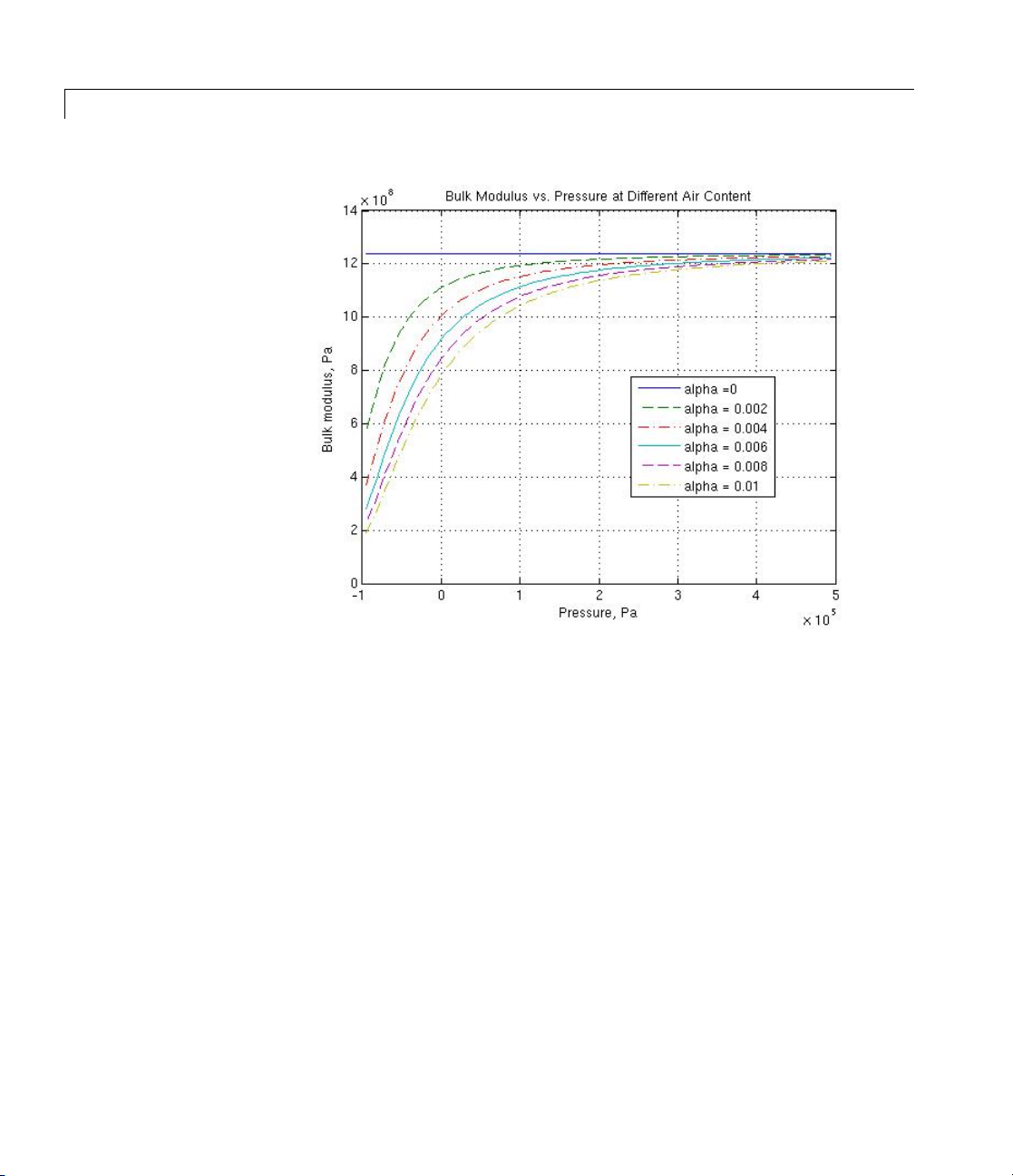
The main objective of representing fluid as a mixture of liquid and gas
is to introduce an approximate model of cavitation, which takes place
in a chamber if pressure drops below fluid vapor saturation level. As
it is seen in the graph below, the bulk modulus of a mixture decreases
at
pp
At high pressure,
, thus considerably slowing down further pressure change.
→
a
pp
>>
, a small amount of nondissolved gas has
a
practically no effect on the system behavior.
2-33
Page 58
Constant Volume Hydraulic Chamber
2-34
Cavitation is an inherently thermodynamic process, requiring
consideration of multiple-phase fluids, heat transfers, etc., and as
such cannot be accurately simulated with Simscape software. But the
simplified version implemented in the block is good enough to signal
if pressure falls below dangerous level, and to prevent computation
failure that normally occurs at negative pressures.
If it is known t hat cavitation is unlikely in the system under design, you
can set the relative gas content in the fluid properties to zero, thus
increasing the speed of computations. Use the Hydraulic Fluid or the
Custom Hydraulic Fluid block to set the fluid properties.
If chamber walls have noticeable compliance , the ab ov e equations must
be further enhanced by representing geometrical chamber volume as a
function of pressure:
Page 59

Constant Volume Hydraulic Chamber
VdL
=π24/ i
c
K
ds
where
() ()=
p
+1 τ
s
ps
d
L
K
p
τ
s
Coefficient
Internal diameter of the cylindrical chamber
Length of the cylindrical chamber
Proportionality coefficient (m/Pa)
Time constant
Laplace operator
K
establishes relationship between press ure and the
p
internal diameter at steady-state conditions. For metal tubes, the
coefficient can be computed as (see [1]):
22
⎛
K
dEDd
=
p
M
+
⎜
22
⎜
Dd
−
⎝
⎞
+
ν
⎟
⎟
⎠
where
D
E
M
Pipe external diameter
Modulus of elasticity (Young’s modulus) for the pipe material
Poisson’s ratio for the pipe material
For hoses, the coefficient can be provided by the manufacturer.
The process of expansion and contraction in pipes and especially in
hosesisacomplexcombinationofnonlinear elastic and viscoelastic
deformations. This process is approximated in the block with the
2-35
Page 60

Constant Volume Hydraulic Chamber
first-order lag, whose time constant is determined empirically (for
example, see [2]).
As a result, by selecting appropriate values, you can implement four
different models of fluid compressibility with this block:
• Chamber with rigid walls, no entrained gas in the fluid
• Cylindrical chamber with compliant walls, no entrained gas in the
fluid
• Chamber with rigid walls, fluid with entrained gas
• Cylindrical chamber with compliant walls, fluid with entrained g as
The block allows two methods of specifying the chamber size:
• By volume — Use this option for cylindrical or non-cylindrical
chambers w ith rigid walls. You only need to know the volume of the
chamber. This chamber type does not account for wall compliance.
• By length and diameter — Use this option for cylindrical chambers
with rigid or compliant walls, such as circular pipes or hoses.
Basic
Assumptions
and
Limitations
2-36
The block has one hydraulic conserving port associated with the
chamber inlet. The block positive direction is from its port to the
referencepoint. Thismeansthattheflowrateispositiveifitflows
into the chamber.
The model is based on the following assumptions:
• No inertia associated with pipe walls is taken into account.
• Chamber with compliant walls is assumed to have a cylindrical
shape. Chamber with rigid wall can ha ve any shape.
Page 61

Dialog
Box a nd
Parameters
Constant Volume Hydraulic Chamber
2-37
Page 62
Constant Volume Hydraulic Chamber
2-38
Page 63

Constant Volume Hydraulic Chamber
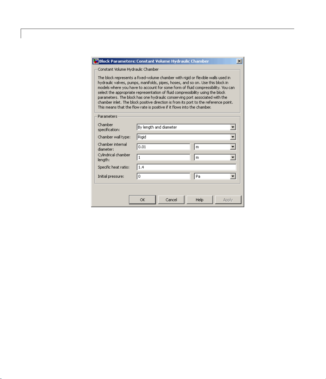
Chamber specification
Theparametercanhaveoneoftwovalues:
length and diameter
recommended if a chamber is formed by a circular pipe. If the
parameter i s set to
account. The default value of the parameter is
Chamber wall type
Theparametercanhaveoneoftwovalues:
If the parameter is set to
account, which can improve computational efficiency. The value
Compliant is recommended for hoses and metal pipes, where
.ThevalueBy length and diameter is
By volume, wall compliance is not taken into
Rigid, wall compliance is not taken into
By volume or By
By volume.
Rigid or Compliant.
2-39
Page 64

Constant Volume Hydraulic Chamber
compliance can affect the system behavior. The default value of
the p arameter is
specification parameter is set to
Chamber volume
Volume of fluid in the chamber. The default value is
The parameter is used if the Chamber specification parameter
is set to
By volume.
Chamber internal diameter
Internal diameter of the cylindrical chamber. The default value is
0.01 m. The parameter is used if the Chamber specification
parameter is set to
Cylindrical chamber length
Length of the cylindrical chamber. The default value is
parameter is used if the Chamber specification param eter is
set to
By length and diameter.
Static pressure-diameter coefficient
Coefficient
the internal diameter at steady-state conditions. The parameter
can be determ ined analytically or experimentally. The default
value is
1.2e-12 m/Pa. The parameter is used if Chamber wall
type is set to
Rigid. The parameter is used if the Chamber
By length and diameter.
K
that establishes relationship between pressure and
p
Compliant.
By length and diameter.
1e-4 m^3.
1 m. The
2-40
Viscoelastic process time constant
Time constant in the transfer function relating pipe internal
diameter to pressure variations. With this parameter, the
simulated elastic or v iscoelastic process is approximated with the
first-order lag. The parameter is determined experimentally or
provided by the manufacturer. The default value is
parameter is used if Chamber wall type is set to
Compliant.
Specific heat ratio
Gas-specific heat ratio. The default value is
1.4.
Initial pressure
Initial pressure in the chamber. This parameter specifies the
initial condition for use in computing the block’s initial state at
0.01 s. The
Page 65

Constant Volume Hydraulic Chamber
the beginning of a simulation run. For more information, see
“Computing Initial Conditions”. The default value is
Restricted Parameters
When your model is in Restricted editing mode, you cannot modify the
following parameters:
• Chamber specification
• Chamber wall type
All other block parameters are available for modification. The actual
set of modifiable block parameters depends on the values of the Tube
cross section type and Chamber wall type parameters at the time
the model entered Restricted mode.
0.
Global
Parameters
Fluidbulkmodulus
The parameter is determined by the type of working fluid selected
for the system under design. Use the Hydraulic Fluid block or the
Custom Hydraulic Fluid block to specify the fluid properties.
Nondissolved gas ratio
Nondissolved gas relative content determined as a ratio of gas
volume to the liquid volume. The parameter is determined by the
type of working fluid se le cted for the system under design. Use
the Hydraulic Fluid block or the Custom Hydraulic Fluid block
to specify the fluid properties.
Ports The block has one hydraulic conserving port associated with the
chamber inlet.
References [1] Meritt, H.E., Hydraulic Control Systems, John Wiley & Sons, N ew
York, 1967
[2] Holcke, Jan, Frequency Response of Hydraulic Hoses, RIT, FTH,
Stockholm, 2002
2-41
Page 66

Constant Volume Hydraulic Chamber
See Also Hydraulic Piston Chamber
Variable Hydraulic Chamber
2-42
Page 67

Constant Volume Pneumatic Chamber
Purpose Simulate constant volume pneumatic chamber based on ideal gas law
Library Pneumatic Elements
Description The Constant Volume Pneumatic Chamber block models a constant
volume pneumatic chamber based on the ideal gas law and assuming
constant specific heats.
The continuity equation for the network representation of the co n stant
chamber is
VRTdpdtpTdT
G
where
G Mass flow rate at input port
⎛
=−
⎜
⎝
dt
⎞
⎟
⎠
V
p
R
T
t
The energy equation is
where
Chamber volume
Absolute pressure in the chamber
Specific gas constant
Absolute gas temperature
Time
cV
v
q
=−i
Rdpdt
q
w
2-43
Page 68

Constant Volume Pneumatic Chamber
Basic
Assumptions
and
Limitations
Dialog
Box a nd
Parameters
q
q
w
c
v
Port A is the pneumatic conserving port associated with the chamber
inlet. Port H is a thermal conserving port through which heat exchange
with the environment takes place. The gas flow a nd the heat flow are
considered positive if they flow into the chamber.
The model is based on the following assumptions:
• The gas is ideal.
• Specific heats at constant pressure and constant volume, c
are constant.
Heat flow due to ga s inflow in the chamber (through the
pneumatic port)
Heat flow through the chamber walls (through the thermal
port)
Specific heat at constant volume
and cv,
p
2-44
Page 69

Constant Volume Pneumatic Chamber
Chamber volume
Specify the volume of the chamber. The default value is
Initial pressure
Specify the initial pressure in the chamber. This parameter
specifies the initial condition for use in computing the initial state
at the beginning of a simulation run. For more information, see
“Computing Initial Conditions”. The default val ue is
Initial temperature
Specify the initial temperature of the gas in the chamber. This
parameter specifies the initial condition for use in computing
the initial state at the beginning of a simulation run. For more
information, see “Computing Initial Conditions”. The default
value is
Ports The block has the following ports:
A
Pneumatic conserving port associated with the chamber inlet.
293.15 K.
.001 m^3.
101235 Pa.
H
Thermal conserving port through which heat exchange with the
environment takes place.
See Also Pneumatic Piston Chamber
Rotary Pneumatic Piston Chamber
2-45
Page 70

Controlled Current Source
Purpose Simulate ideal current source driven by input signal
Library Electrical Sources
Description The Controlled Current Source block repres ents an ideal current source
that is powerful enough to maintain the specified current through it
regardless of the voltage across the source.
The output current is I=Is,whereIs is the numerical value presented
at the physical signal port.
The p ositive direction of the current flow is indicated by the arro w.
Dialog
Box a nd
Parameters
The block has no parameters.
Ports The block has one physical signal input port and two electrical
conserving ports associated with its electrical terminals.
See Also Controlled Voltage Source
2-46
Page 71

Controlled Flux Source
Purpose Simulate ideal flux source driven by input signal
Library Magnetic Sources
Description The Controlled Flux Source block represents an ideal flux source that is
powerful enough to maintain the specified flux through it regardless of
the mmf across the source.
The output flux is PHI = PHIs,wherePHIs is the numerical value
presented at the physical signal port.
The positive direction of the flux flow is indicated by the arrow.
Dialog
Box a nd
Parameters
The block has no parameters.
Ports The blo
conse
ck has one physical signal input port and two magnetic
rving ports associated with its magnetic terminals.
See Also Controlled MMF Source
Flux Source
MMF Source
2-47
Page 72

Controlled MMF Source
Purpose Simulate ideal magnetomotive force source driven by input signal
Library Magnetic Sources
Description The Controlled MMF Source block represents an ideal magnetomotive
force (mmf) source that is powerful enough to maintain the specified
mmf at its output regardless of the flux passing through it.
The output mmf is MMF = MMFI,whereMMFI is the numerical value
presented at the physical signal port.
Dialog
Box a nd
Parameters
The block has no parameters.
Ports The block has one physical signal input port and two magnetic
conserving ports associated with its magnetic terminals.
See Also Controlled Flux Source
Flux Source
MMF Source
2-48
Page 73
Controlled Pneumatic Flow Rate Source
Purpose Simulate ideal compressor with signal-controlled mass flow rate
Library Pneumatic Sources
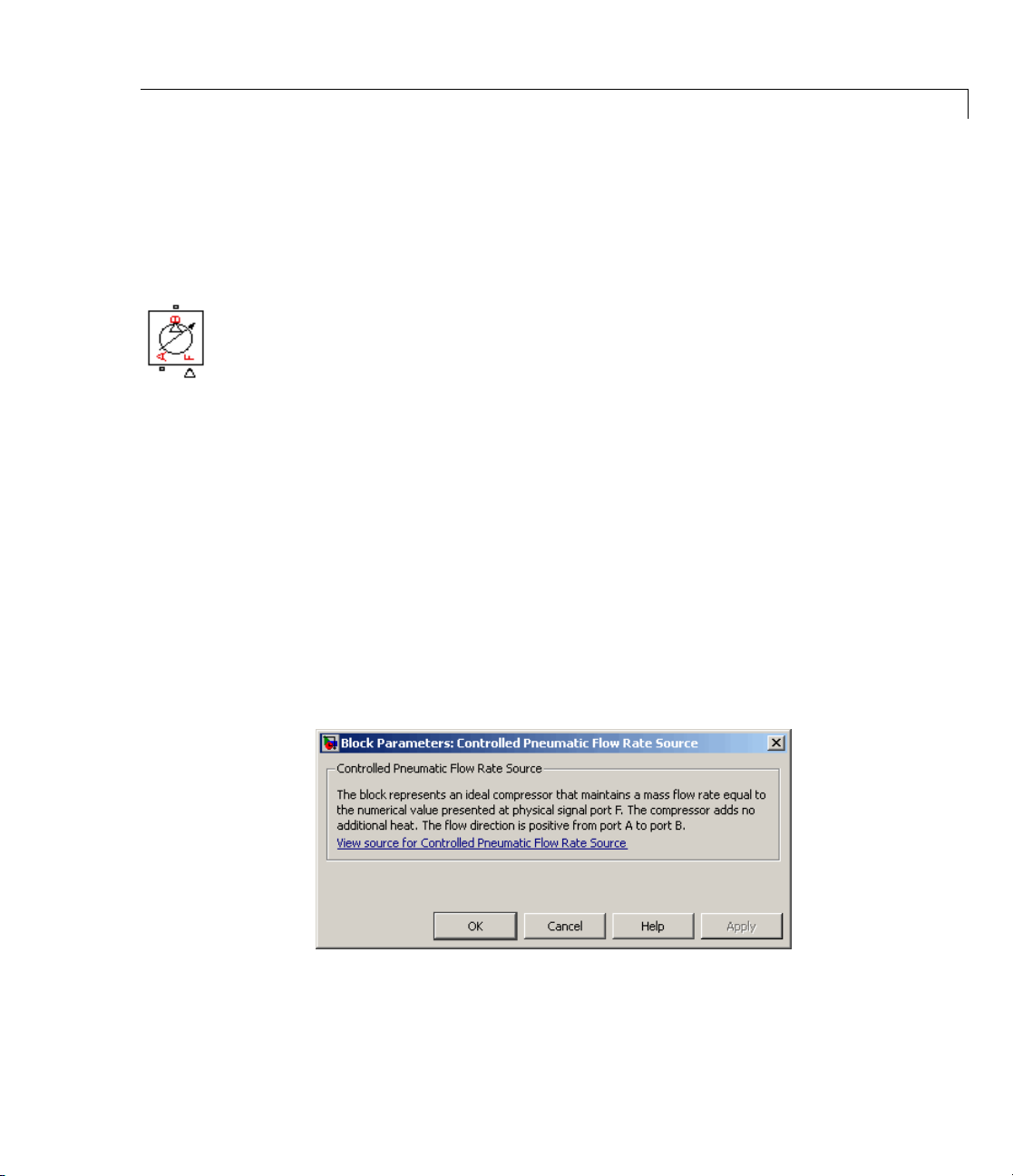
Description The Controlled Pneumatic Flow Rate Source block represents an ideal
compressor that maintains a mass flow rate equal to the numerical
value presented at physical signal port F. The compressor adds no heat.
Block connections A and B correspond to the pneumatic inlet and outlet
ports, respectively, and connection F represents a control signal port.
The block positive direction is from port A to port B. This means that
theflowrateispositiveifitflowsfromAtoB.Thepressuredifferential
is determined as p=p
outlet is greater than pressure at its inlet. The power generated by the
source is negative if the source adds energy to the flow.
Warning
Be careful w hen driving an orifice directly from a flow rate
source. The choked flow condition limits the flow that is
possible through an orifice as a function of upstream pressure
and temperature. Hence the flow rate value produced by the
flow rate source must be compatible with upstream pressure
and temperature. Specifying a flow rate that is too h igh will
result in an unsolvable set of equations.
and is negative if press ure at the source
A–pB
Dialog
Box a nd
Parameters
The block has no parameters.
2-49
Page 74

Controlled Pneumatic Flow R ate Source
Ports The block has the following ports:
A
Pneumatic conserving port associated with the source inlet.
B
Pneumatic conserving port associated with the source outlet.
F
Control signal port.
See Also Pneumatic Flow Rate Source
Pneumatic Mass & Heat Flow Sensor
2-50
Page 75

Controlled Pneumatic Pressure Source
Purpose Simulate ideal compressor with signal-controlled pressure difference
Library Pneumatic Sources
Description The Controlled Pneumatic Pressure Source block represents an ideal
compressor that maintains a pressure difference equal to the numerical
value presented at physical signal port F. The compressor adds no heat.
Block connections A and B correspond to the pneumatic inlet and outlet
ports, respectively, and connection F represents a control signal port.
A positive pressure difference results in the pre ssu re at port B being
higher than the pressure at port A.
Dialog
Box a nd
Parameters
The block has no parameters.
Ports The block has the following ports:
A
Pneumatic conserving port associated with the source inlet.
B
Pneumatic conserving port associated with the source outlet.
F
Control signal port.
2-51
Page 76

Controlled Pneumatic Pressure Source
See Also Pneumatic Pressure Source
Pneumatic Pressure & Temperature Sensor
2-52
Page 77

Controlled Voltage Source
Purpose Simulate ideal voltage source driven by input signal
Library Electrical Sources
Description The Controlled Voltage Source block represents an ideal voltage source
that is powerful enough to maintain thespecifiedvoltageatitsoutput
regardless of the current flowing through the source.
The output current is V=Vs,whereVs is the numerical value presented
at the physical signal port.
Dialog
Box a nd
Parameters
The block has no parameters.
Ports The block has one physical signal input port and two electrical
conserving ports associated with its electrical terminals.
See Also Controlled Current Source
2-53
Page 78
Convective Heat Transfer
Purpose Simulate heat transfer by convection
Library Thermal Elements
Description TheConvectiveHeatTransferblock represents a heat transfer by
convection between two bodies by means of fluid motion. T he transfer
is governed by the Newton law of cooling and is described with the
following equation:
QkAT T
=−ii()
where
Q Heat flow
AB
k
A
T
A,TB
Connections A and B are thermal conserving ports associated with the
points between which the heat transfer by convection takes place. The
block positive direction is from port A to port B. This means that the
heat flow is positive if it flows from A to B.
Convection heat transfer coefficient
Surface area
Temperatures of the bodies
2-54
Page 79

Dialog
Box a nd
Parameters
Convective Heat Transfer
Area
Surface area of heat transfer. The d efault value is
Heat transfer coefficient
Convection heat transfer coefficient. Th e default value is
W/m^2/K.
0.0001 m^2.
20
Ports The block has the following ports:
A
Thermal conserving port associated with body A .
B
Thermal conserving port associated with body B .
See Al
so
Condu
Radia
ctive Heat Transfer
tive Heat Transfer
2-55
Page 80

Current-Controlled Current Source
Purpose Simulate linear current-controlled current source
Library Electrical Sources
Description The Current-Controlled Current Source block models a linear
current-controlled current source, described with the following equation:
IKI21= i
where
Dialog
Box a nd
Parameters
I2
K
I1
To use the block, connect the + and – ports on the left side of the block
(the control ports) to the control current source. The arrow between
these p orts indicates the positive direction of the control current flow.
The two ports on the right side of the block (the output ports) generate
the output current, with the arrow between them indicating the positive
direction of the output current flow.
Output current
Current gain
Current flowing from the + to the – control port
2-56
Page 81

Current-Controlled Current Source
Current gain K
Ratio of the current between the two output terminals to the
current passing between the two control terminals. The default
value is
Ports The block has four electrical conserving ports. Connections + and – on
the left side of the block are the control ports. The other two ports are
the electrical terminals that provide the output current. The arrows
between each pair of ports indicate the positive direction of the current
flow.
See Also Current-Controlled Voltage Source
Voltage-Controlled Current Source
Voltage-Controlled Voltage Source
1.
2-57
Page 82

Current-Controlled Voltage Source
Purpose Simulate linear current-controlled voltage source
Library Electrical Sources
Description The Current-Controlled Voltage Source block models a linear
current-controlled voltage source, described with the following equation:
VKI= i 1
where
Dialog
Box a nd
Parameters
V
K
I1
To use the block, connect the + and – ports on the left side of the block
(the control ports) to the control current source. The arrow indicates the
positive direction of the current flow. The two ports on the right side
of the block (the output ports) generate the output voltage. Polarity
is indicated by the + and – signs.
Transresistance K
Voltage
Transresistance
Current flowing from the + to the – control port
Ratioofthevoltagebetweenthe two output terminals to the
current passing between the two control terminals. The default
value is
1 Ω.
2-58
Page 83

Current-Controlled Voltage Source
Ports The block has four electrical conserving ports. Connections + and –
on the left side of the block are the control ports. The arrow indicates
the positive direction of the current flow. The other two ports are
the electrical terminals that provide the output voltage. Polarity is
indicated by the + and – signs.
See Also Current-Controlled Current Source
Voltage-Controlled Current Source
Voltage-Controlled Voltage Source
2-59
Page 84

Current Sensor
Purpose Simulate current sensor in electrical systems
Library Electrical Sensors
Description The Current Sensor block represents an ideal current sensor, that is,
a device that converts current measured in any electrical branch into
a physical signal proportional to the current.
Connections + and – are electrical conserving ports through which the
sensor is inserted into the circuit. Connection I is a physical signal port
that outputs the measurement result.
Dialog
Box a nd
Parameters
Ports The blo
2-60
The block has no parameters.
ck has t he following ports:
+
rical conserving p ort associated with the sensor positive
Elect
nal.
termi
-
trical conserving port associated with the sensor negative
Elec
inal.
term
Page 85

I
Physical signal output port for current.
See Also Voltage Sensor
Current Sensor
2-61
Page 86

Custom Hydraulic Fluid
Purpose Set working fluid properties by specifying parameter values
Library Hydraulic Utilities
Description The Custom Hydraulic F luid block lets you specify the type of hydraulic
fluid used in a loo p of hydraulic blocks. It provides the hydraulic fluid
properties, such as kinematic viscosity, density, and bulk modulus, for
all the hydraulic blocks in the loop. These fluid properties are assumed
to be constant during simulation time.
The Custom Hydraulic Fluid block lets you specify the fluid properties,
such as kinematic viscosity, density, bulk modulus, and relative amount
of entrapped air, as block parameters.
The Custom Hydraulic Fluid block has one port. You can connect it to
a hydraulic diagram by branching a connection line off the main line
and connecting it to the port. When you connect the Custom Hydraulic
Fluid block to a hydraulic line, the software automatically identifies the
hydraulic blocks connected to the particular loop and propagates the
hydraulic fluid properties to all the hydraulic blocks in the loop.
2-62
Each topologically distinct hydraulic loop in a diagram requires exactly
one Custom Hydraulic Fluid block or Hydraulic Fluid block , available
with SimHydraulics libraries, to be connected to it. Therefore, there
must be as many Custom Hydraulic Fluid blocks (or Hydraulic Fluid
blocks) as there are loops in the system.
Note If no Hydraulic Fluid block or Custom Hydraulic Fluid block is
attached to a loop, the hydraulic blocks in this loop use the default fluid,
which is Skydrol LD-4 at 60°C and with a 0.005 ratio of entrapped air.
See the Hydraulic Fluid block reference page for more information.
Page 87

Dialog
Box a nd
Parameters
Custom Hydraulic Fluid
Fluid density
Density of the working fluid. The default value is 850 kg/m^3.
Kinematic viscosity
Kinematic viscosity of the working fluid. The default value is
1.8e-5 m^2/s.
Bulk modulus at atm. pressure and no gas
Bulk modulus of the working fluid, at atmospheric pressure and
with no entrapped air. The default value is 8e8 Pa.
Relative amount of trapped air
Amount of entrained, nondissolved gas in the fluid. The amount
is specified as the ratio of gas volume at normal conditions to the
fluid volume in the chamber. If set to 0, ideal fluid is assumed.
The default value is 0.005.
Ports The block has one hydraulic conserving port.
See Also Hydraulic Fluid
2-63
Page 88

DC Current Source
Purpose Simulate ideal constant current source
Library Electrical Sources
Description The DC Current Source block represents an ideal current source that
is powerful enough to maintain specified current through it regardless
of the voltage across the s ource.
You specify the output current by using the Constant current
parameter, which can be positive or negative.
The p ositive direction of the current flow is indicated by the arro w.
Dialog
Box a nd
Parameters
Constant current
Output current. You can specify positive or negative values. The
default value is
1 A.
Ports The block has two electrical conserving ports associated with its
terminals.
See Also DC Voltage Source
2-64
Page 89

DC Voltage Source
Purpose Simulate ideal constant voltage source
Library Electrical Sources
Description The DC Voltage Source block represents an ideal voltage source that is
powerful enough to maintain specified voltage at its o u tput regardless
of the current flowing through the source.
You specify the output voltage by using the Constant voltage
parameter, which can be positive or negative.
Connections + and – are conserving electrical ports corresponding to the
positive and negative terminals of the voltage source, respectively. The
current is positive if it flows from positive to negative, and the voltage
across the source is equal to the difference between the voltage at the
positive and the negative terminal, V(+) – V(–).
Dialog
Box a nd
Parameters
Constant voltage
Output voltage. You can specify positive or negative values. The
default value is
1 V.
Ports The block has the following ports:
+
Electrical conserving port associated with the source positive
terminal.
2-65
Page 90

DC Voltage Source
-
Electrical conserving port associated with the source negative
terminal.
See Also DC Current Source
2-66
Page 91

Diode
Purpose Simulate piecewise linear diode in electrical systems
Library Electrical Elements
Description The Diode block models a piecewise linear diode. If the voltage across
the diode is bigger than the Forward voltage parameter value, then
the diode beha ves like a linear resistor with low res ista nce, given by
the On resistance parameter value, plus a series voltage source. If the
voltageacrossthediodeislessthantheforwardvoltage,thenthediode
behaves like a linear resistor with low conductance given by the Off
conductance parameter value.
When forward biased, the series voltage source is described with the
following equation:
VVf R G
=−()1 i
where
on off
V
Vf
R
on
G
off
The R
Voltage
Forward voltage
On resistance
Off conductance
.
G
term ensures that the diode current is exactly zero when
on
off
the voltage across it is zero.
2-67
Page 92

Diode
Dialog
Box a nd
Parameters
Forward voltage
Minimumvoltagethatneedstobeappliedforthediodetobecome
forward-biased. The default value is
On resistance
Theresistanceofaforward-biaseddiode. Thedefaultvalueis
0.3 Ω.
0.6 V.
Off conductance
The conductance of a reverse-biased diode. The default value is
1e-8 1/Ω.
Ports The block has the following ports:
+
Electrical conserving port associated with the diode positive
terminal.
-
Electrical conserving port associated with the diode negative
terminal.
2-68
Page 93

Electrical Reference
Purpose Simulate connection to electrical ground
Library Electrical Elements
Description The Electrical Reference block represents an electrical ground.
Electrical conserving ports of all the blocks that are directly connected
to ground must be connected to an Electrical Reference block. A m odel
with electrical elements must contain at least one Electrical Reference
block.
Dialog
Box a nd
Parameters
The Electrical Reference block has no parameters.
Ports The bloc
k has one electrical conserving port.
See Also Hydraulic Reference
Mechanical Rotational Reference
Mechanical Translational Reference
Thermal Reference
2-69
Page 94

Electromagnetic Converter
Purpose Simulate lossless electromagnetic energy conversion device
Library Magnetic Elements
Description The Electromagnetic Converter block provides a generic interface
between the electrical and magnetic domains.
The block is based on the following equations:
F =⋅NI
d
VN
=− ⋅
where
Φ
dt
Basic
Assumptions
and
Limitations
F
Φ
I
V
N
t
Connections N and S are magnetic conserving ports, and connections +
and – are electrical conserving ports. If the current from the electrical +
to – ports is positive, then the resulting mmf is positive acting across
the magnetic N to S ports. A positive rate of change of flux flowing from
N to S results in a negative induced voltage across the + and – ports.
The model is based on the following assumption:
• Electromagnetic energy conversion is lossless.
Magnetomotive force (mmf) a cros s the magnetic ports
Flux through the magnetic ports
Current through the electrical ports
Voltage across the electrical ports
Number of electrical winding turns
Simulation time
2-70
Page 95
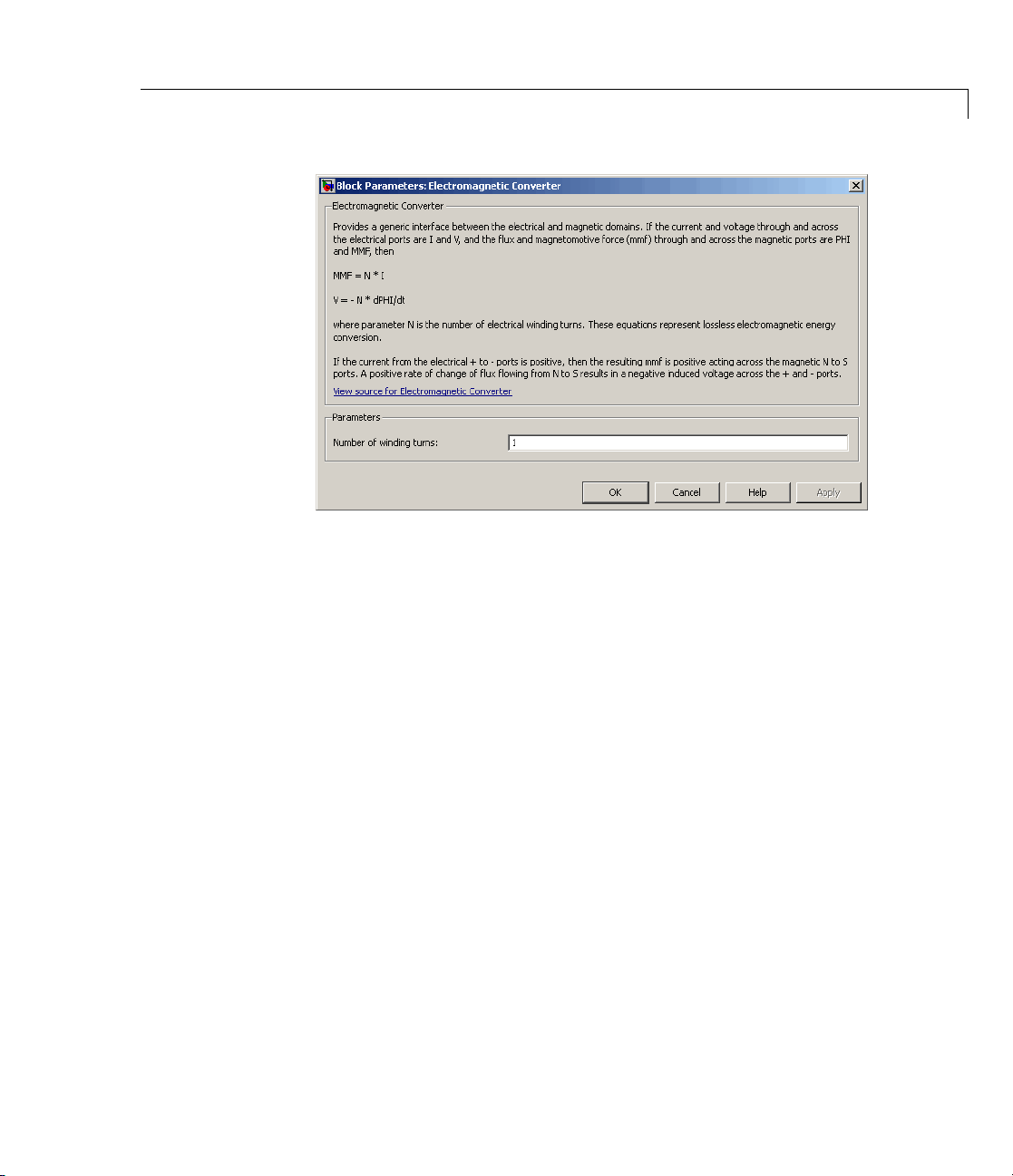
Dialog
Box a nd
Parameters
Electromagnetic Converter
Number of winding turns
Number of electrical winding turns. The default value is
1.
Ports The block has the following ports:
N
Magnetic conserving port associated with the block North
terminal.
S
Magnetic conserving port associated with the block South
terminal.
+
Positive electrical conserving port.
-
Negative electrical conserving port.
See A
lso
ctance Force Actuator
Relu
2-71
Page 96

Fluid Inertia
Purpose Simulate pressure differential across tube or channel due to change
in fluid velocity
Library Hydraulic Elements
Description The Fluid Inertia block models pressure differential, due to change in
fluid velocity, across a fluid passage of constant cross-sectional area.
The pressure differential is determined according to the following
equation:
LAdq
p
=ρ
dt
where
Assumptions
and
Limitations
p
ρ
L
A
q
t
Use this block in various pipe or channel models that require fluid
inertia to be accounted for.
The block positive direction is from port A to port B. This means that
theflowrateispositiveifitflowsfromAtoB.
The model is based on the following assumptions:
• Fluid density remains constant.
Pressure differential
Fluid density
Passage length
Passage area
Flow rate
Time
2-72
Page 97

Dialog
Box a nd
Parameters
Fluid Inertia
a
ge cross-sectional area. The default value is
ngth
he fluid passage. The default value is
low rate
low rate through the passage. This parameter specifies
al condition for use in computing the b lock’s initial state
inning of a simulation run. For more information, see
ing Initial Conditions”. The default value is
Global
Parameters
Passage are
Fluid passa
Passage le
Length of t
Initial f
Initial f
the initi
at the beg
“Comput
Fluid density
The parameter is determined by the type of working fluid selected
for the system under design. Use the Hydraulic Fluid block or the
Custom Hydraulic Fluid block to specify the fluid properties.
Ports The block has the following ports:
A
Hydraulic co nserving port asso ciated with the passage inlet.
B
Hydraulic conse rving port associate d with the passage outlet.
8e-5 m^2.
1 m.
0.
2-73
Page 98
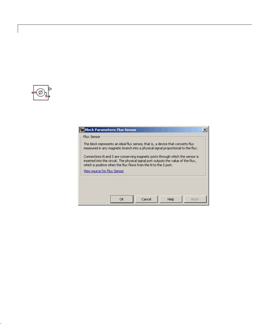
Flux Sensor
Purpose Simulate ideal flux sensor
Library Magnetic Sensors
Description The Flux Sensor block represents an ideal flux sensor, that is, a device
that converts flux measured in any magnetic branch into a physical
signal proportional to the flux.
Connections N and S are conserving magnetic ports through which the
sensor is inserted into the circuit. The physical signal port outputs the
value of the flux, w hich is positive when the flux flows from the N to
the S port.
Dialog
Box a nd
Parameters
The block has no parameters.
Ports The block has the following ports:
N
Magnetic conserving port associated with the sensor N orth
terminal.
2-74
Page 99

S
Magnetic conserving port associated with the sensor South
terminal.
The block also has a physical signal output port, which outputs the
value of the flux.
See Also Controlled Flux Source
Flux Source
Flux Sensor
2-75
Page 100

Flux Source
Purpose Simulate ideal flux source
Library Magnetic Sources
Description The Flux Source block represents an ideal flux source that is powerful
enough to maintain specified constan t flux through it, regardless of the
mmf across its terminals.
You specify the output flux by using the Constant flux parameter,
which can be positive, negative, or zero .
You can also model permanent magnets with this block, using the
following equation:
Constant flux = Gauss strength * Cross-sectional area
The positive direction of the flux flow is indicated by the arrow.
Dialog
Box a nd
Parameters
Constant flux
Output flux. You can specify any real value. The default value
is
0.001 Wb.
Ports The block has two magnetic conserving ports associated with its
terminals.
2-76
 Loading...