Mathworks SIMPOWERSYSTEMS 5 user guide

Download

SimPowerSystems™ 5

User’s Guide

Hydro-Québec

How to Contact The MathWorks

www.mathworks. comp.soft-sys.matlab Newsgroup www.mathworks.com/contact_TS.html T echnical Support

suggest@mathworks.com Product enhancement suggestions

bugs@mathwo doc@mathworks.com Documentation error reports service@mathworks.com Order status, license renewals, passcodes

info@mathwo

com

rks.com

Web

Bug reports

Sales, prici

ng, and general information

508-647-7000 (Phone)

508-647-7001 (Fax)

The MathWorks, Inc. 3 Apple Hill Drive Natick, MA 01760-2098

For contact information about worldwide offices, see the MathWorks Web site.

SimPowerSystems™ User’s Guide

The software desc ribed in this docu ment is furnished under a license ag reement. The software may be used or copied only under the terms of the license agreement. No part of this manual may be photocopied or reproduced in any form without prior written consent from The MathWorks, Inc.

FEDERAL ACQUISITION: This provision applies to all acquisitions of the Program and Documentation by, for, or through the federal government of the United States. By accepting delivery of the Program or Docum entation, the government hereby agrees tha t this software or documentation qualifies as commercial computer software or commercial computer software documentation as such terms are used or defined in FAR 12.212, DFARS Part 227.72, and DFARS 252.227-7014. Accordingly, the terms and conditions of this Agreement and only those rights specified in this Agreement, shall pertain to and govern theuse,modification,reproduction,release,performance,display,anddisclosureoftheProgramand Documentation by the federal government (or other entity acquiring for or through the federal governme nt) and shall supersede any conflicti ng contractual terms or conditions. If this License fails to meet the government’s needs or is inconsistent in any respect with federal procurement law, the government agrees to return the Program and Documentation, unused, to The MathWorks, Inc.

Trademarks

MATLAB and Simulink are registered trademarks of The MathWorks, Inc. See

www.mathworks.com/trademarks for a list of additional trademarks. Other product or brand

names may be trademarks or registered trademarks of their respective holders.

Patents

The MathWorks products are protected by one or more U.S. patents. Please see

www.mathworks.com/patents for more information.

Revision History

January 1998 First printing Version 1.0 (Release 10) September 2000 Second printing Revised for Version 2.1 (Release 12) June 2001 Online only Revised for Version 2.2 (Release 12.1) July 2002 Online only Revised for Version 2.3 (Release 13) (Renamed from Power

System Blockset User’s Guide) February 2003 Third printing Revised for Version 3.0 (Release 13SP1) June 2004 Online only Revised for Version 3.1 (Release 14) October 2004 Fourth printing Revised for Version 4.0 (Release 14SP1) March 2005 Online only Revised for Version 4.0.1 (Release 14SP2) May 2005 Online only Revised for Version 4.1 (Release 14SP2+) September 2005 Online only Revised for Version 4.1.1 (Release 14SP3) March 2006 Online only Revised for Version 4.2 (Release 2006a) September 2006 Online only Revised for Version 4.3 (Release 2006b) March 2007 Online only Revised for Version 4.4 (Release 2007a) September 2007 Online only Revised for Version 4.5 (Release 2007b) March 2008 Online only Revised for Version 4.6 (Release 2008a) October 2008 Online only Revised for Version 5.0 (Release 2008b) March 2009 Online only Revised for Version 5.1 (Release 2009a) September 2009 Online only Revised for Version 5.2 (Release 2009b) March 2010 Online only Revised for Version 5.2.1 (Release 2010a)

Acknowledgments

SimPowerSystems™ software was developed by the following people and organizations.

Gilbert Sybille

Hydro-Québec Research Institute (IREQ), Varennes, Québec. Original author of SimPowerSystems software, technical coordinator, author of the Ideal Switching Solution Method, autho r of phasor simulation, discretization techniques, and documentation. Technical supervision and design of the FACTS and Distributed Resources libraries , and documentation.

Louis-A. Dessaint

École de Technologie Supérieure (ETS), Montréal, Québec. Author of machine models. Technical supervision and design of the electric drive library contents, and documentation.

Bruno DeKelper

École de Technologie Supérieure (ETS), Montréal, Québec. Author of the Ideal Switching Solution Method and author of TLC functions associated with the simulation of the state space equations.

Olivier Tremblay, Jean-Roch Cossa

École de Technologie Supérieure (ETS), M o n tré al, Q u ébec. Validations and tests of the Ideal Sw itching Solution Method.

Patrice Brunelle

Hydro-Québec Research Institute (IREQ), Varennes, Québec. Main software engineer. Author of graphical user interfaces, model integration into Simulink

and Physical Modeling, and documentation.

Acknowledgments

Roger Champagne

École de Technologie Supérieure (ETS), Montréal, Québec. Author of machine models, of revised state space fo rmulation. Design of the graphical user interface of the electric drive library.

Pierre Giroux, Richard Gagnon, Silvano Casoria

Hydro-Québec Research Institute (IREQ), Varennes, Québec. Development of the FACTS and Distributed R esources libraries. Key beta testers and developers of several SimPowerSystems blocks, demos, and documentation.

Hoang Lehuy

Université Laval, Québec City. Validation tests and author of several models, functions, and documentation. Validation of the electric drives library.

Handy Fortin-Blanchette, Olivier Tremblay, Christophe Semaille

École de Technologie Supérieure (ETS), Montréal, Québec. Development of the AC and DC drives models.

Hassan Ouquelle, Jean-Nicolas Paquin

École de Technologie Supérieure (ETS), Montréal, Québec. Development of the Single-Phase Asynchronous Machine model and Saturation in Asynchronous Machine model.

Pierre Mercier

iOMEGAt. Project manager for the Power System Blockset™ software versions 1 and 2 and for the Simulink electric drives library.

The authors acknowledge the contributions of the following people:

Innocent Kamwa, Raymond Roussel, Kamal Al-Haddad, Mohamed Tou, Christian Dufour, Momcilo Gavrilovic, Christian Larose, David McCallum, Bahram Khodabakhchian, Manuel Alvarado Sandoval, and Stéphane Desjardins

Acknowledgments

Getting Started

Product Overview ................................. 1-2

Introduction TheRoleofSimulationinDesign SimPowerSystems Libraries Required and Related Products

...................................... 1-2

..................... 1-2

........................ 1-3

...................... 1-4

Contents

Using This Guide

If You Are a New User If You Are an Experienced Blockset User All Users Units

Building and Simulating a Simple Circuit

Introduction Building the Electrical Circuit with powerlib Library Interfacing the Electrical Circuit with Other Simulink

Blocks Measuring Voltages and Currents Basic Principles of Connecting Capacitors and Inductors Using the Powergui Block to Simulate SimPowerSystems

Models

Analyzing a Simple Circuit

Introduction Electrical State Variables State-Space Representation Using power_analyze Steady-State Analysis Frequency Analysis

........................................ 1-6

........................................... 1-6

........................................ 1-13

........................................ 1-16

.................................. 1-5

............................. 1-5

.............. 1-5

........... 1-7

...................................... 1-7

.................... 1-14

......................... 1-18

...................................... 1-18

........................... 1-18

.............................. 1-19

................................ 1-21

.... 1-8

.. 1-15

....... 1-19

vii

Specifying Initial Conditions ....................... 1-27

Introduction State Variables Initial States Specify Initial Electrical States with Powergui

...................................... 1-27

................................... 1-27

..................................... 1-28

.......... 1-29

Simulating Transients

Introduction Simulating Transients with a Circuit B reaker Continuous, Variable Time Step Integration Algorithms Discretizing the Electrical System

Introducing the Phasor Simulation Method

Introduction When to Use the Phasor Solution Phasor Simulation of a Circuit Transient

...................................... 1-33

...................................... 1-40

............................. 1-33

.......... 1-33

.................... 1-37

.......... 1-40

.................... 1-40

.............. 1-41

Advanced Components and Techniques

Introducing Power Electronics ..................... 2-2

Introduction Simulation of the TCR Branch Simulation of the TSC Branch

Simulating Variable Speed Motor Control

Introduction Building and Simulating the PWM Motor Drive Using the Multimeter Block Discretizing the PWM Motor Drive Performing Harmonic Analy sis Using the FFT Tool

...................................... 2-2

....................... 2-4

....................... 2-8

........... 2-11

...................................... 2-11

......... 2-13

......................... 2-19

................... 2-21

.. 1-35

..... 2-21

viii Contents

Three-Phase Systems and Machines

Introduction Three-Phase Network with Electrical Machines Load Flow and Machine Initialization Using the Phasor Solution Method for Stability Studies

...................................... 2-25

................. 2-25

................. 2-28

......... 2-25

.. 2-36

Building and Customizing Nonlinear Models ......... 2-40

Introduction Modeling a Nonlinear Inductance Customizing Your Nonlinear Model Modeling a Nonlinear Resistance Creating Your Own Library Connecting Your Model with Other Nonlinear Blocks

Building a Model Using Model Construction

Commands

...................................... 2-40

.................... 2-40

................... 2-45

..................... 2-48

......................... 2-53

...................................... 2-57

Improving Simulation Performance

How SimPowerSystems Software Works ............. 3-2

.... 2-53

Choosing an Integration Method

Introduction Continuous Versus Discrete Solution Phasor Solution Method

Simulating with Continuous Integration Algorithms

Choosing an Integration Algorithm Simulating Switches and Power Electronic Devices Using the Ideal Switching Device Method

Simulating Discretized Electrical Systems

Introduction Limitations of Discretization with Nonlinear Models

Simulating Power Electronic Models

Introduction Circuit Using Forced-Commutated Power Electronics Circuit Using Naturally Commutated Power Electronics

Increasing Simulation Speed

Ways to Increase Simulation Speed

...................................... 3-4

............................ 3-5

...................................... 3-15

...................................... 3-17

.................... 3-4

................. 3-4

................... 3-6

...... 3-7

.............. 3-8

........... 3-15

..... 3-15

................ 3-17

....................... 3-19

................... 3-19

.. 3-6

.... 3-17

.. 3-17

Using Accelerator Mode and Real-Time Workshop

Software

....................................... 3-19

The Nonlinear Model Library

HowtoAccesstheNonlinear Model Library The Continuous Library The Discrete Library The Phasors Library The Switch Current Source Library Limitations of the Nonlinear Models Modifying the Nonlinear Models of the powerlib_ m odels

Library

Creating Your Own Library of Models

Changing Your Circuit Parameters

Introduction Example of MATLAB Script Performing a Parametric

Study

........................................ 3-24

...................................... 3-26

......................................... 3-26

............................ 3-22

............................... 3-23

Systems with Electric Driv es

....................... 3-22

............ 3-22

................... 3-23

.................. 3-23

............... 3-25

.................. 3-26

x Contents

About the Electric Drives Library ................... 4-2

Getting Started with Electric Drives Library

What Is an Electric Drive? Three Main Components of an Electric Drive Multiquadrant Operation Average-Value Models User Interface General Layout of the Library’s GUIs Features of the New GUIs Advanced Usage

Simulating a DC Motor Drive

Introduction Regenerative Braking

.................................... 4-9

.................................. 4-12

...................................... 4-13

.......................... 4-4

........................... 4-7

............................. 4-8

................. 4-9

.......................... 4-10

....................... 4-13

.............................. 4-14

......... 4-4

........... 4-4

Example: Thyristor Converter-Based DC Motor Drive ... 4-14

Simulating an AC Motor Drive

Introduction Dynamic Braking Modulation Techniques Open-Loop Volts/Hertz Control Closed-Loop Speed Control with Slip Compensation Flux-Oriented Control Direct Torque Control Example: AC Motor Drive

Mechanical Models

Mechanical Shaft Block Speed Reducer Block

Mechanical Coupling of Two Motor Drives

Introduction System Description Speed Regulated AC4 with Torque Regulated DC2 Torque Regulated AC4 with Speed Regulated DC2

Winding Machine

Introduction Description of the Winder Block Description Simulation Results

...................................... 4-39

................................. 4-39

............................. 4-40

.............................. 4-46

.............................. 4-49

................................ 4-69

............................ 4-69

............................... 4-70

...................................... 4-71

................................ 4-72

.................................. 4-78

...................................... 4-78

................................. 4-80

................................ 4-83

...................... 4-39

...................... 4-45

.......................... 4-50

........................... 4-78

..... 4-46

........... 4-71

...... 4-74

...... 4-75

Robot Axis Control Using Brushless DC Motor Drive

Introduction Description of the Robot Manipu la tor Position Control Systems for Joints 1 and 2 Modeling the Robot Position Control Systems Tracking Performance of the Motor Drives

Building Your Own Drive

Introduction Description of the Drive Modeling the Induction Motor Drive Starting the Drive Steady-State Voltage and Current Waveforms

...................................... 4-86

................. 4-86

............ 4-87

.......... 4-88

............. 4-92

.......................... 4-97

...................................... 4-97

............................ 4-98

.................. 4-100

................................. 4-104

.......... 4-105

.. 4-86

Speed Regulation Dynamic Performance ............... 4-106

Advanced Users: Retune the Drive P a ra m ete rs

Modify the Motor Parameters Retune the Parameters of the Flux Regulator Retune the Parameters of the Speed Regulator Retune the Parameters of the DC Bus Voltage Simulate and Analyze the Results

Advanced Users: Modify a Drive Block

Disable the Drive Link Modify the Electrical Connections Simulate the Sys tem and Observe the R esults

Multi-Level Modeling for Rapid Prototyping

Introduction The System Architecture The Simplified Model The Average-Value Model The Detailed Model Comparison of the Multi-Level Modeling Precision Conclusion

...................................... 4-130

....................................... 4-150

............................. 4-123

.............................. 4-132

................................ 4-142

....................... 4-108

.......... 4-109

.......... 4-119

.................... 4-122

.............. 4-123

.................... 4-124

.......... 4-128

........................... 4-131

........................... 4-135

....... 4-108

......... 4-115

......... 4-130

...... 4-145

xii Contents

Transients and Power Electronics in Power

Series-Compensated Transmission System ........... 5-2

Description of the Transmission System Setting the Initial Load Flow and Obtaining Steady

State

.......................................... 5-8

Transient Performance for a Line Fault Frequency Analysis TransientPerformanceforaFaultatBusB2

Thyristor-Based Static Var Compensator

Introduction Description of the SVC

...................................... 5-20

................................ 5-13

............................. 5-21

............... 5-2

............... 5-9

........... 5-16

............ 5-20

Systems

Steady-State and Dynamic Performance of the SVC ..... 5-24

Misfiring of TSC1

................................. 5-26

GTO-Based STATCOM

Introduction Description of the STATCOM Steady-State and Dynamic Performance of the

STATCOM

Thyristor-Based HVDC Link

Description of the HVDC Transmission System Frequency Response of the AC and DC Systems Description of the Control and Protection Systems System Startup/Stop — Steady-State and Step

Response DC Line Fault AC Line-to-Ground Fault at the Inverter

VSC-Based HVDC Link

Introduction Description of the HVDC Link VSC Control System Dynamic Performance

...................................... 5-29

..................................... 5-36

...................................... 5-48

.................................... 5-54

...................................... 5-61

............................. 5-29

........................ 5-30

........................ 5-39

.............. 5-57

............................. 5-61

....................... 5-61

............................... 5-65

.............................. 5-71

......... 5-39

........ 5-41

...... 5-43

Transient Stability of Power Systems Using

Phasor Simulation

Transient Stability of a Power System with SVC and

PSS

Introduction Description of the Transmission System Single-Phase Fault — Impact of PSS — No SVC Three-Phase Fault — Impact of SVC — PSS in Service

Control of Power Flow Using a UPFC and a PST

Introduction Description of the Power System Power Flow Control with the UPFC

............................................ 6-2

...................................... 6-2

............... 6-2

...................................... 6-9

..................... 6-9

.................. 6-12

........ 6-4

... 6-6

..... 6-9

xiii

UPFC P-Q Controllable Region ...................... 6-13

Power Flow Control Using a PST

..................... 6-14

Wind Farm Using Doubly-Fed Induction Generators

Description of the Wind Farm TurbineResponsetoaChangeinWindSpeed Simulation of a Voltage Sag on the 120 kV System Simulation of a Fault on the 25 kV System

....................... 6-19

.......... 6-23

...... 6-25

............. 6-27

.. 6-19

Index

xiv Contents

Getting Started

• “Product Overview” on page 1-2

• “Using This Guide” on page 1-5

• “Building and Simulating a Simple Circuit” on page 1- 7

• “Analyzing a Simple Circuit” on page 1-18

• “Specifying Initial Conditions” on page 1-27

• “Simulating Transients” on page 1-33

• “Introducing the Phasor Simulation Method” on page 1-40

1 Getting Started

Product Overview

Introduction

SimPowerSystems software and other products of the Physical Modeling product family work together with Simulink software to model electrical, mechanical, and control s ystem s.

SimPowerSystems software operates in the Simulink environment. Therefore, before starting this user’s guide, make yourself familiar with Simulink documentation. Or, if you perform signal processing and communications tasks (as opposed to control system design tasks), see the Signal Processing Blockset™ documentation.

In this section...

“Introduction” on page 1-2 “The Role of Simulation in Design” on page 1-2 “SimPowerSystems Libraries” on page 1-3 “Required and Related Products” on page 1-4

1-2

TheRoleofSimulationinDesign

Electrical power systems are combinations of electrical circuits and electromechanical devices like motors and generators. Engineers working in this discipline are constantly improving the performance of the s ystem s. Requirements for dra stica lly increased efficiency have forced power system designers to use power electronic devices and sophisticated control system concepts that tax traditional analysis tools and techniques. Further complicating the analyst’s role is the fact that the system is often so nonlinear that the only way to understand it is through simulation.

Land-based power generation from hydroelectric, steam, or other devices is not the only use of power system s. A common attribute of these system s is their use of power electronics and control systems to achieve their performance objectives.

Product Overview

SimPowerSystems software is a modern design tool that allows scientists and engineers to rapidly and easily build models that simulate power systems. It uses the Simulink environment, allowing you to build a model using simple click and drag procedures. Not only can you draw the circuit topology rapidly, but your analysis of the circuit can include its interactions with mechanical, thermal, control, and other disciplines. This is possible because all the electrical parts of the simulation interact with the extensive Simulink modeling library. Since Simulink uses the MATLAB

computational engine, designers can also use MATLAB toolboxes and Simulink blocksets. SimPowerSystems software belongs to the Physical M odeling product family and uses similar block and connection line interface.

SimPowerSystems Libraries

SimPowerSystems libraries contain models of typical power equipment such as transformers, lines, machines, and power ele ctronics. These models are proven one s coming from textbooks, and their validity is based on the experience of the Power Systems Testing and Simulation Laboratory of Hydro-Québec, a large North American utility located in Canada, and also on the experience of École de Technologie Supérieure and Université Laval. The capabilities of SimPowerSystems software for modeling a typical electrical system are illustrated in demonstration files. And for users who w an t to refresh their knowledge of power system theory, there are also self-learning case studies.

The SimPowerSystems main library, powerlib, organizes its blocks into libraries according to their behavior. The powerlib library window displa ys the block library icons and names. Double-click a library icon to open the library and access the blocks. The main powerlib library window also contains the Pow erg u i block that opens a graphical user interface for the steady-state analysis of electrical circuits.

Nonlinear Simulink Blocks for SimPowerSystems Models

The nonlinear Simulink blocks of the powerlib library a re stored in a special block library named powerlib_models. These masked Simulink models are used by SimPowerSystems software to build the equivalent Simulink model of your circuit. See Chapter 3, “Improving Simulation Performance” for a description of the powerlib_models library.

1-3

1 Getting Started

Required and Rel

SimPowerSystem

• MATLAB

• Simulink

In addition to family includ and electric systems in Si toolboxes a with SimPow products, s the “Produc

ee the MathWorks Web site at

s software requires the following products:

SimPowerSystems software, the Physical Modeling product

es other products for modeling and simulating mechanical

al systems. Use these products together to model physical

mulink environment. There are also a number of closely related

nd other products from The MathWorks™ that you can use

erSystems software. For more information about any of these

ts” section.

ated Products

http://www.mathworks.com;see

1-4

Using This Guide

In this section...

“If You Are a New User” on page 1-5 “If You Are an Experienced Blockset User” on page 1-5 “All Users” on page 1-6 “Units” on page 1-6

If You Are a New User

Begin with this chapter and also the next chapter to learn how to

• Build and simulate electrical circui ts using the powerlib library

• Interface an electrical circuit with Simulink blocks

• Analyze the steady-state and frequency response of an electrical circuit

Using This Guide

• Discretize your model to increase simulation speed, especially for power

electronic circuits and large power systems

• Use the phasor simulation method

• Build your own nonlinear models

If You Are an Experienced Blockset User

See the Release Notes for details on the latest release.

Also, see these chapters:

• Chapter 1, “Getting Started” to learn how to simulate discretized electrical

circuits

• Chapter 2, “Advanced Components and Techniques” to learn how to apply

the phasor simulation to transient stability study of multimachine systems

• Chapter 3, “Improving Simulation Performance” to learn how to increase

simulation speed

1-5

1 Getting Started

All Users

For reference in use the SimPower

formation on blocks, simple demos, and G UI-based tools,

Systems Reference.

For commands, r syntax, as wel

l as a complete explanation of options and operation.

Units

This guide us system. See T

es the International System of Units (SI) and the per unit (pu)

echnical Conventions for details.

efer to “Function Reference” for a synopsis of the command

1-6

Building and Simulating a Simple Circuit

In this section...

“Introduction” on page 1-7 “Building the Electrical Circuit with powerlib Library” on page 1-8 “Interfacing the Electrical Circuit with Other Simulink Blocks” on page 1-13 “Measuring Voltages and Currents” on page 1-14 “Basic Principles of Connecting Capacitors and Inductors” on page 1-15 “Using the Powergui Block to Simulate SimPowerSystems Models” on page

1-16

Introduction

SimPowerSystems software allows you to build and simulate electrical circuits containing linear and nonlinear elem ents.

Building and Simulating a Simple Circuit

In this section you

• Explore the powerlib library

• Learn how to build a sim ple circuit from the powerlib library

• Interconnect Sim u l in k blocks with your circuit

The circuit below represe nts an equivalent power system feeding a 300 km transmission line. The line is compensated by a shunt inductor at its receiving end. A circuit breaker allows energizing a nd de-energizing of the line. To simplify matters, only one of the three phases is represented. The parameters shown in the figure are typical of a 735 kV power system.

1-7

1 Getting Started

CircuittoBeModeled

Building the Electrical Circuit with powerlib Library

The graphical user interface makes use of the Simulink functionality to interconnect various electrical components. The electrical components are grouped in a library called powerlib.

1 Open the SimPowerSystems main library by entering the following

command at the MATLAB prompt.

1-8

powerlib

This command displays a Simulink window showing icons of different block libraries.

You can open these libraries to produce the windows containing the blocks to be copied into your circuit. Each component is represented by a special icon having one or several inputs and outputs corresponding to the different terminals of the component:

2 From the File menu of the powerlib window, open a new window to

contain your first circuit and save it as

3 Open the Electrical Sources library and copy the AC Voltage Source block

into the circuit1 window.

circuit1.

Building and Simulating a Simple Circuit

4 Open the AC Voltage Source dialog box by double-clicking the icon and

enter the Amplitude, Phase, and Frequency parameters according to the valuesshowninCircuittoBeModeledonpage1-8.

Note that the amplitude to be specified f or a sinusoidal source is its p eak value (424.4e3*sqrt(2) volts in this case).

5 Change the name of this block from AC Voltage Source to Vs.

6 Copy the Parallel RLC Branch block, which can be found in the Elements

library of powerlib, set its parameters as shown in Circuit to Be Modeled on page 1-8, and n ame it Z_eq.

7 The resistance Rs_eq of the circuit can be obtained from the Parallel RLC

Branch block. Duplicate the Parallel RLC Branch block, which is already in your circuit1 window. Select R for the Branch Type parameter and set the R parameter according to Circuit to Be M odeled on page 1-8.

Once the dialog box is closed, notice that the L and C components have disappeared so that the icon now shows a single resistor.

Note With the Branch Type parameter set to RLC, setting L and C respectively to

inf and zero in a parallel branch changes automatically the

Branch Type to R and produces the same result. Similarly, with the Series RLC Branch block, setting R, L, and C respectively to zero, zero, and

inf

eliminates the corresponding element.

8 Name this block Rs_eq.

9 Resize the various components and interconnect blocks by dragging lines

from outputs to inputs of appropriate blocks.

1-9

1 Getting Started

10 To complete the circuit of Circuit to Be Modeled on page 1 -8, you need to

add a transmission line and a shunt reactor. You add the circuit breaker later in “Simulating Transients” on page 1-33.

The model of a line with uniformly distributed R, L, and C parameters normally consists of a delay equal to the wave propagation time along the line. This model cannot be simulated as a linear system because a delay corresponds to an infinite number of states. However, a good approximation of the line with a finite number of states can be obtained by cascading several PI circuits, each representing a small section of the line.

1-10

A PI section consists of a series R-L branch and two shunt C branches. The model accuracy depends on the number of PI sections used for the model. Copy the PI Section Line block from the Elements library into the circuit1 window, set its parameters as shown in Circuit to Be Modeled on page 1-8, andspecifyonelinesection.

11 The shunt reactor is modeled b y a resistor in serie s with an inductor. You

could use a Series RLC Branch block to model the shunt reactor, but then you would have to manually calculate and set the R and L values from the quality factor and reactive power specified in Circuit to Be Modeled on page 1-8.

Therefore, you might find it more convenient to use a Series RLC Load block that allows you to specify directly the active and re active powers absorbed by the shunt reactor.

Copy the Series RLC Load block, w h ich can be found in the Elements library of powerlib. Name this block 110 Mvar. Set its parameters as follows:

Building and Simulating a Simple Circuit

424.4e3 V

60 Hz 110e6/300 W (quality factor = 300) 110e6 vars

Note th at, as no reactive capacitive po w er is specified, the capacitor disappears o n the block icon when the dialog box is closed. Interconnect the newblocksasshown.

12 You need a Voltage Measurement block to measure the voltage at node B1.

This block is found in the Measurements library of powerlib.Copyitand name it U1. Connect its positive input to the node B1 and its negative input to a new Ground block.

13 To observe the voltage measured by the Voltage Measurement block

named U1, a display system is needed. This can be any device found in the Simulink Sinks library.

OpentheSinkslibraryandcopytheScopeblockintoyourcircuit1 window. If the scope were connected directly at the output of the voltag e measurement, it would display the voltage in volts. However, electrical engineers in pow er systems are used to working with normalized quantities (per unit system). The voltage is normalized by dividing the v alue in volts by a base voltage corresponding to thepeakvalueofthesystemnominal voltage. In this case the scaling factor K is

1-11

1 Getting Started

K =

424 4 10 2

14 Copy a Gain block from the Simulink library and set its gain as above.

××

Connect its output to the Scope block and connect the output of the Voltage Measurement block to the Gain bl ock . Duplicate this voltage measurement system at the node B2, as shown below.

15 Add a Powergui block to your model. The purpose of this block is discussed

in “Using the Powergu i Block to Simulate SimPowerSystems Models” on page 1-16.

1-12

16 From the Simulation menu, select Start.

17 Open the Scope blocks and o bs erve the voltages at nodes B1 and B2.

18 While the simulation is running, open the Vs block dialog box and modify

the amplitude. Observe the effect onthetwoscopes. Youcanalsomodify the frequency and the phase. You can zoom in on the waveforms in the scope windows by drawing a box around the region of interest with the left mouse button.

To simulate this circuit, the default integration algorithm (

ode45)wasused.

However, for most SimPowerSystems applications, your circuits contain switches and other nonlinear models. In such a case, you must specify a

Building and Simulating a Simple Circuit

different integration algorithm. This is discussed in “Simulating Transients” on page 1-33, where a circuit breaker is added to your circuit.

Interfacing the Electrical Circuit with Other Simulink Blocks

The Voltage Measurement block acts as an interface between the SimPowerSystems blocks and the Simulink blocks. For the system shown above, you implemented such an interface from the electrical system to the Simulink system. The Voltage Measurement block converts the measured voltages into Sim ulink signals.

Similarly, the Current Measurement block from the Measurements library of powerlib can be used to convert any measured current into a Simulink signal.

You can also interface from Simulink blocks to the electrical system. For example, you can use the Controlled Voltage Source block to inject a voltage in an electrical circuit, as shown in the following figure.

1-13

1 Getting Started

Electrical Terminal Ports and Connection Lines SimPowerSystems

modeling environment is similar to that of other products in the Physical Modeling family. Its blocks often feature both normal Simulink input and output ports

> and special electrical terminal ports :

• Lines that connect normal Simulink ports

• Lines that connect terminal ports

These lines are nondirectional and can be branched, but you cannot connect them to Simulink ports > or to normal Simulink signal lines.

• You can connect Simulink ports

electrical terminal ports

• Converting Simulink signals to electrical connections or vice versa requires

using a SimPowerSystems block that features both Simulink ports and electrical terminal ports.

Some SimPowerSystems blocks feature only one type of port.

only to other electrical terminal ports.

are special electrical connection lines.

> only to othe r Simulink ports and

> are directional signal lines.

Measuring Voltages and Currents

When you measure a current using a Current Measurement block, the positive direction of current is indicated on the block icon (positive current flowing from + terminal to – terminal). Similarly, when you measure a voltage using a Voltage Measurement block, the measured voltage is the voltage of the + terminal w ith respect to the – terminal. However, when voltages and currents of blocks from the Elements library are measured using the Multimeter block, the voltage and current polarities are not immediately obvious because blocks might have been rotated and there are no signs indicating polarities on the block icons.

1-14

Unlike Simulink signal lines and input and output ports, the SimPowerSystems connection lines and terminal ports directionality. The voltage and current polarities are determined, not by line direction, but instead by block orientation. To find out a block orientation, first click the block to select it. Then enter the following command.

get_param(gcb,'Orientation')

lack intrinsic

Building and Simulating a Simple Circuit

The following table indicates the polarities of the currents and voltages measured with the Multimeter block for single-phase and three-phase RLC branch and loads (and of the polarity of the capacitor voltage and the inductor current), surge arresters, and single-phaseandthree-phasebreakers.

Positive Current

Block Orientation

right

left

down

The natural orientation of the blocks (that is, their orientation in the Element library) is right for horizontal blocks and down for vertical blocks.

For single-phase transformers (linear or saturable), with the winding connectors appearing on the left and right sides, the winding voltages are the voltages of the top connector with respect to the bottom connector, irrespective of the block orientation (right or left). The winding currents are the currents entering the top connector.

Direction Measured Voltage

left —> right Vleft – Vright right —> left Vright – Vleft top —> bottom Vtop – Vbottom bottom —> top Vbottom – Vtop

For three-phase transformers, the voltage polarities and positive current directions are indicated by the signal labels used in th e Multimeter block. For example, Uan_w2 means phase A-to-ne utral voltage o f the Y connected winding #2 , Iab_w1 me an s winding current flowing from A to B in the delta-connected winding #1.

Basic Principles of Connecting Capacitors and Inductors

You have to pay particular attention when you connect cap a c itor elements together with voltage sources, or inductor elements in series with current sources. When you start the simulation, the software displays an error message if one of the following two connection errors are present in your diagram:

1-15

1 Getting Started

1 You have connected a voltage source in parallel with a capacitor, or a series

of capacitor elements in series, like in the two examples below.

To fix this problem, y ou can a dd a small resistance in series between the voltage source and the capacitors.

2 You have connected a current source in series with an inductor, or a s eries

of inductors connected in parallel, like in the example below.

1-16

To fix t induct

Using SimPo

The P cont Simu Sim

You

his problem, you can add a large re sistance in parallel with the

or.

the Powergui Block to Simulate

werSystems Models

owergui block is necessary for simulation of any Simulink model

aining SimPowerSystems blocks. It is use d to store the equivalent

link circuit that represents the state-space equations of the

PowerSystems blocks.

must follow these rules when using this block in a m o del:

Building and Simulating a Simple Circuit

• Place the Powergui block at the top lev el of diagram for optimal

performance. However, you can place it anywhere inside subsystems for your convenience; its functionality will not be affected.

• You can have a maximum of one Powerg ui block per m ode l

• You must name the block

powergui

Note When you start the simulation, yo u will get an error if no Powergui block is found in your model.

1-17

1 Getting Started

Analyzing a Simple Circuit

In this section...

“Introduction” on page 1-18 “Electrical State Variables” on page 1-18 “State-Space Representation Using power_analyze” on page 1-19 “Steady-State Analysis” on page 1-19 “Frequency Analysis” on page 1-21

Introduction

In this section you

• Obtain the state-space representation of your model with the

power_analyze comm and

• Compute the steady-state voltages and currents using the graphical user

interface of the Powergui block

1-18

• Analyze an electrical circuit in the frequency domain

Electrical State Variables

The electrical state variables are the Simulink states of your diagram associated to the capacitor and inductor devices of the SimPowerSystems blocks. Inductors and capacitors elements are found in the RLC-branch type blocks such as the Series RLC Branch block, Three-Phase Parallel RLC Load block, in the transformer models, in the PI Section Line block, in the snubber devices of the power e lectronic devices, etc.

The electrical state variables consist of the inductor currents and the capacitor voltages. Variable names forSimPowerSystems electrical states contain the name of the block where the inductor or capacitor i s found, preceded b y the

Il_ prefix for inductor currents or the Uc_ prefix for capacitor voltages.

Analyzing a Simple Circuit

State-Space Rep

You compute the s

power_analyze c

resentation Using power_analyze

tate-space representation of the model

ommand. Enter the following command at the MATLAB

circuitl with the

prompt.

[A,B,C,D,x0,electrical_states,inputs,outputs]=power_analyze('circuit1')

lyze

The power_ana the four matr electrical s inputs, and o

electrical_states =

Il_110 Mvars Uc_input PI Section Line Il_ sect1 PI Section Line Uc_output PI Section Line Il_Z_eq Uc_Z_eq

inputs =

U_Vs

ices A, B, C, and D. x0 is the vector of initial conditions of the

tates of your circuit. The names of the electrical state variables,

utputs are returned in three string matrices.

command returns the state-space model of your circuit in

outputs =

U_U1 U_U2

hat you could have obtained the names and ordering of the electrical

Note t

es, inputs, and outputs directly from the Powergui block. See the

stat

r_analyze

powe

ady-State Analysis

Ste

acilitate the ste ad y-state analysis of your circuit, the powerlib library

To f

ludes a graphical user interface tool. If the Powergui block is not already

inc

sent in your model, copy the block from the library into your circuit1

pre

del and double-click the block icon to open it.

reference page for more details on how to use this function.

1-19

1 Getting Started

From the Analysis tools menu of the Powergui block, select Steady-State Voltages and Currents. This opens the Steady-State Tool window where

thesteady-statephasorsvoltagesmeasuredbythetwovoltagemeasurement blocks of your model are displayed in polar form.

1-20

Eachmeasurementoutputisidentified b y a string corresponding to the measurement block name. The magnitudes of the phasors U1 and U2 correspond to the peak value of the sinusoidal voltages.

From the Steady-State Tool window, you can also display the steady-state values of the source voltage or the steady-state values of the inductor currents and capacitor voltages by selecting either the Sources or the States check box.

Analyzing a Simple Circuit

Note Depending on the order you added the blocks in your circuit1 diagram, the electrical state variables might not be ordered in the same way as in the preceding figure.

Refer to the section “Measuring Voltages and Currents” on page 1-14 for more details on the sign conventions used for the voltages and currents of sources and electrical state variables listed in the Steady-State Tool window.

Frequency Analysis

The Measurements library of powerlib contains an Impedance Measurement block that measures the impedance between any two nodes of a circuit. In the following two sections, you measure the impedance of your circuit between node B2 and ground by using two methods:

• Calculation from the state-space m odel

• Automatic measurement using the Impedance Measurement block and the

Powergui block

1-21

1 Getting Started

Obtaining the Impedance vs. Frequency Relation from the State-Space Model

Note The following section assumes you have Control System Toolbox™

software installed.

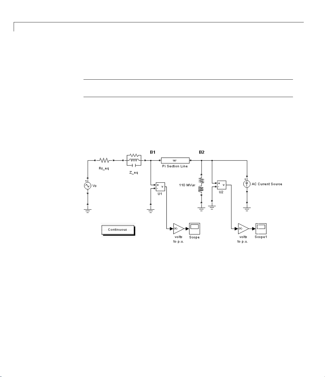
To measure the impedance versus frequency at node B2, you need a current source at node B2 providing a second input to the state-space model. Open the Electrical Sources library and copy the AC Current Source block into your model. Connect this source at node B2, as shown below. Set the current source magnitude to zero and keep its frequency at blocks as follows.

60 Hz. Rearrange the

1-22

AC Current Source at the B2 Node

Now compute the state-space representation of the model circuitl with the

power_analyze command. Enter the following command at the MATLAB

prompt.

sys1 = power_analyze('circuit1','ss')

This command returns a state-space model representing the continuous-time state-space model of your electrical circuit.

Analyzing a Simple Circuit

IntheLaplacedomain,theimpedanceZ2atnodeB2isdefinedasthetransfer function between the current injected by the AC current Source block and the voltage measured by the U2 Voltage Measurement block.

()

You obtain the names of the inputs and outputs of this state-space model as follows.

sys1.InputName ans =

'U_Vs'

'I_AC Current Source' sys1.OutputName ans =

'U_U2'

'U_U1'

The impedance at node B2 then corresponds to the transfer function between output 1 and input 2 of this state-space model. For the 0 to 1500 Hz range, it can be calculated and displayed as follows.

freq=0:1500; w=2*pi*freq; bode(sys1(1,2),w);

Repeat the same process to get the frequency response with a 10 section line model. Open the PI Section Line dialog box and change the number of sections from

1 to 10. To calculate the new frequency response and

superimpose it upon the one obtained with a single line section, enter the following commands.

sys10 = power_analyze('circuit1','ss'); bode(sys1(1,2),sys10(1,2),w);

Open the property editor of the Bode plot and select units for Frequency in H z using linear scale and Magnitude in absolute using log scale. The resulting plot is shown below.

1-23

1 Getting Started

Impedance at Node B2 as Function of Frequency

This graph indicates that the frequency rangerepresentedbythesingleline section model is limited to approximately 150 Hz. For higher frequencies, the 10 line section model is a better approximation.

1-24

The system with a single PI section has two oscillatory modes at 89 Hz and 229 Hz. The 89 Hz m ode is due to the equivalent source, which is modeled by a single pole equivalent. The 229 Hz mode is the first mode of the line modeled by a single PI section.

For a distributed parameter line model the propagation speed is

The propagation time for 300 km is therefore T = 300/293,208 = 1.023 ms and the frequency of the first line mode is f1 = 1/4T = 244 Hz. A distributed parameter line would have an infinite number of modes every 244 + n*488 Hz (n=1,2,3...). The10sectionlinemodelsimulatesthefirst10modes. The first three line modes can be seen in Impedance at Node B2 as Function of Frequency on page 1-24 (244 Hz, 732 Hz, and 1220 Hz).

⋅

=1293 208,/

km s=

Analyzing a Simple Circuit

Obtaining the Impedance vs. Frequency Relation from the Impedance Measurement and Powergui Blocks

The process described above to measure a circuit impedance has been automated in a SimPowerSystems block. Open the Measurements library of powerlib, copy the Impedance Measurement block into your model, and rename it ZB2. Connect the two inputs of this block between node B2 and ground as shown.

Measuring Impedance vs. Frequency with the Impedance Measurement Block

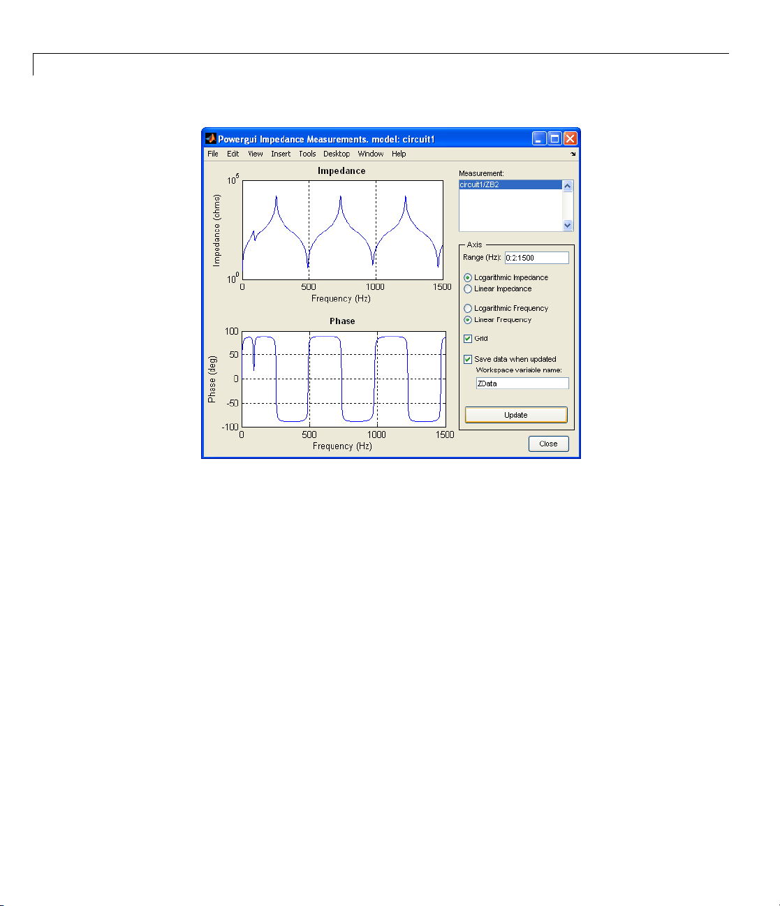
Now open the Powergui dialog. In the Tools menu, select Impedance vs Frequency Measurement. A new window opens, showing the list of

Impedance Measurement blocks available in your circuit.

In your case, only one impedance is measured, and it is identified by ZB2 (the name of the ZB2 block) in the window. Fill in the frequency range by en ter in g

0:2:1500 (zero to 1500 Hz by steps of 2 Hz). Select the logarithmic scale to

display Z magnitude. Select the Save data when updated check box and enter

ZData as the variable name to contain the impedance vs. frequency.

Click the Update button.

1-25

1 Getting Started

1-26

When the phase as plot (fo Freque variab column

r one line section) shown in Impedance at Node B2 as Function of ncy on page 1-24. If you look in your workspace, you should have a

le named

1 and complex impedance in column 2.

calculation is finished, the window displays the ma gnitude and

functions of frequency. The m agnitude should be identical to the

ZData. It is a two-column matrix containing frequency in

Specifying Initial Conditions

In this section...

“Introduction” on page 1-27 “State Variables” on page 1-27 “Initial States” on page 1-28 “Specify Initial Electrical States with Powergui” on page 1-29

Introduction

In this section you

• Learn what are the state variables of a Simulink diagram containing SimPowerSystems blocks

• Specify initial conditions for the electrical state variables

Specifying Initial Conditions

State Variables

The state variables of a Simulink diagram containing SimPowerSystems blocks consist of

• The electrical states associated to RLC branch-type SimPowerSystems blocks. They are defined by the state-space representation of your m odel. See “Electrical State Variables” on page 1 -18 for more details about the electrical states.

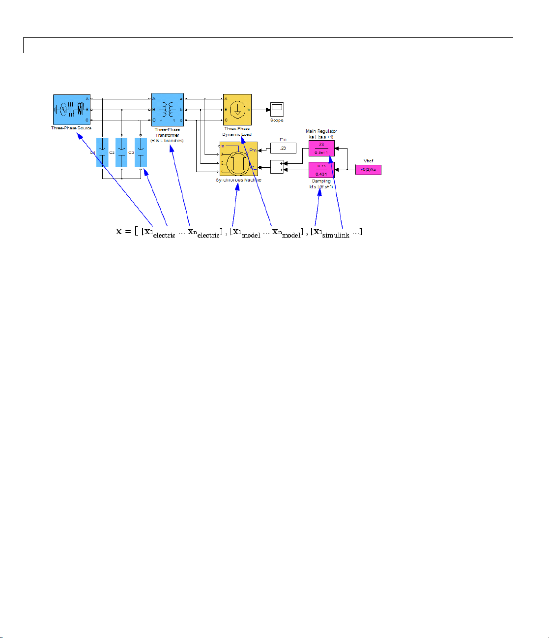
• The Simulink states of the SimPowerSystems electrical models such as the Synchronous Machine block, the Saturable Transformer block, or the Three-Phase Dynam ic Load block.

• The Simulink states of the other Simulink blocks of your model (controls, user-defined blocks, and other blocksets).

The following picture provides an example that contains the three types of state variables:

1-27

1 Getting Started

Initial States

Initial conditions, which are applied to the entire system at the start of the simulation, are generally set in the blo ck s. Most of the Simulink blocks allow you to specify initial conditions. For the case of the electrical states, the SimPowerSystems software automaticall y sets the initial values of the electrical states to start the simulation in steady state.

1-28

However, you can specify the initial conditions for the capacitor voltage and inductor currents in the mask of these blocks:

• the Series and Parallel RLC Branch blocks

• the Series and Parallel RLC Load blocks

The initial values entered in the mask of these block will overwrite the default steady-state parameters calculated by the SimPowe rSystem s software. In the same sense, you can overwrite initial conditions of the overall blocks by specifying them in the States area of the Configuration Parameters dialog box.

See the specify initial states for a Simulink diagram with SimPowerSystems blocks.

power_init function reference page for moredetailsonhowyoucan

Specifying Initial Conditions

Specify Initial Electrical States with Powergui

1 Open the Transient Ana lys is of a Linear Circuit demo by typing

power_transient at the comm and line. Rename the RLC Branch blocks

asshowninthenextfigure.

2 From the Analysis tools menu of the Powergui block, select Initial State

Settings. The initial values of the five electrical state variables (three

inductor currents and two capacitor voltages) are displayed. These initial values corresponds to the values that the software automatically sets to start the simulation in steady state.

1-29

1 Getting Started

1-30

3 Open the Scope block and start the simulation. As the electrical state

variables are automatically initialized, the system starts in steady state and sinusoidal waveforms are observed.

4 The initial value for STATE_D state is set to 1.589e5 V. It corresponds to the

initial capacitor voltage found in the

STATE_D block. Open this block, select

the Set the initial capacitor voltage parameter, then specify a capacitor initial voltage of -2e5 V. Click the OK button.

5 Click the From diagram button of the Powergui Initial States Tool to

refresh the display of initial states. The initial state of

STATE_D block is

now set to -2e5 V.

6 Start the simulation. In the second trace of the Scope block, z oom around

the transient at the beginning of the simulation. As expected, the model does not start in steady state, but the initial value for the capacitor voltage measured by the Voltage Measurement block is -2e5 V.

Specifying Initial Conditions

7 Select the STATE_A state variable in the Initial States Tool list. In t he

Set selected electrical state field, set the initial inductor current to 50 A, and click Apply.Openthemaskofthe

STATE_A block, and note that the

Set the initial inductor current parameter is selected and the initial inductor current is set to 50 A.

Run the simulation and observe the new transient caused by this new setting.

Forcing Initial States to Zero

Now suppose that you want to reset all the initial electrical states to zero without loosing the settings you have done in the previous steps.

1 From the Initial State Tool window, select the To zero check box under

Force initial electrical states,thenclickApply. Restart the simulation

and observe the transient when all the initial conditions starts from zero.

2 Open the masks of the STATE_C and STATE_A blocks and note that even if

initial conditions are still specified in these blocks, the setting for the initial states is forced to zero by the Powergui block.

A message is displayed at the command l ine to remind you every time you start the simulation that the e lectrical initial states of your model are forced to zero by the Powergui block, which overwrites the block settings in your model.

Forcing Initial States to Steady State

Similarly, you can set all the initial states to steady without loosing the settings you have done in the previous steps.

1 From the Initial State Tool window , select the To steady state check box

under Force initial electrical states,thenclickApply.

2 Restart the simulation and observe that the simulation starts in steady

state.

A message is displayed at the command line to remind you every time you start the simulation that the electrical initial states of your model are forced to steady state by the Powergui block.

1-31

1 Getting Started

Returning to Block Settings

To return to the block settings, clear both check boxes under Force initial electrical states,thenclickApply.

1-32

Simulating Transients

In this section...

“Introduction” on page 1-33 “Simulating Transients with a Circuit Breaker” on page 1-33 “Continuous, Variable Time Step Integration Algorithms” on page 1-35 “Discretizing the Electrical System” on page 1-37

Introduction

In this section you

• Learn how to create an electrical subsystem

• Simulate transients with a circuit breaker

• Compare time domain simulation results with different line models

Simulating Transients

• Learn how to discretize a circuit and compare results thus obtained with results from a continuous, variable time step algorithm

Simulating Transients with a Circuit Breaker

One of the main uses of SimPowerSystems software is to simulate transients in electrical circuits. This can be done with either mechanical switches (circuit breakers) or switches using power electronic devices.

First open your node B2. Save this new system as breaker, you need to modify the schematic diagram of group several components into a subsystem. This feature is useful to simplify complex schematic diagrams.

Use this feature to transform the source impedance into a subsystem:

1 Select the two blocks identified as Rs_eq and Z_eq by surrounding them by

a box with the left mouse button and use the Edit > Create subsystem menu item. The two blocks now form a new block called Subsystem.

circuit1 system and delete the current source connected at

circuit2. Before connecting a circuit

circuit2.Youcan

1-33

1 Getting Started

2 Using the Edit > Mask subsystem menu item, change the icon of that

subsystem. In the Icon section of the mask editor, enter the following drawing command:

disp('Equivalent\nCircuit')

The icon now reads Equivalent Circuit, as shown in the figure above.

1-34

3 Use the Format > Show drop shadow menu item to add a drop shado w

to the Subsystem block.

4 You can double-click the Subsystem block and look at its content.

5 Insert a circuit breaker into your circuit to sim ulate a line energization by

opening the Elements library of powerlib.CopytheBreakerblockinto your circuit2 window.

The circuit breaker is a nonlinear element modeled by an ideal switch in series with a resistance. Because of modeling constraints, this resistance cannot be set to zero. However, it can be set to a very small value, say 0.001 Ω, that does not affect the performance of the circuit:

1 Open the Breaker block dialog box and set its parameters as follows:

Ron

Initial state

0.001 Ω

0 (open)

inf

Simulating Transients

Switching times

2 Insert the circuit breaker in series with the sending end of the line, then

[(1/60)/4]

rearrange the circuit as shown in the previous figure.

3 Open the scope U2 and click the P ara me te rs icon and select the Data

history tab. Click the Save data to workspace button and specify a

variable name

U2 to save the simulation results; then change the Format

option for U2 to be Array.Also,clearLimit data points to last to display the entire waveform for long simulation times.

You are now ready to simulate your system.

Continuous, Variable Time Step Integration Algorithms

Open the PI section Line dialog box and make sure the num ber of sections is set to 1. Open the Simulation > Configuration Parameters dialog box. As you now have a system containing switches, you need a stiff integration algorithm to simulate the circuit. In the Solver pane, select the variable-step stiff integration algorithm

ode23tb.

Keep the default parameters (relative tolerance set at time to

0.02 seconds. Open the scopes and start the simulation. Look at

1e-3) and set the stop

the waveforms of the sending and receiving en d voltages on ScopeU1 and ScopeU2.

Once the simulation is complete, copy the variable

U2 into U2_1 by entering

the following command in the MATLAB Command Window.

U2_1 = U2;

These two variables now contain the waveform obtained with a single PI section line model.

1-35

1 Getting Started

Open the PI section Line dialog box and change the number of sections from

1 to 10. Start the simulation. Once the simulation is complete, copy

the variable

U2 into U2_10.

Before modifying your circuit to use a distributed parameter line m odel, save your system as

circuit2_10pi, which you can reuse later.

Delete the PI section line model and replace it with a single-phase D istributed Parameter Line block . S et the number of phases to

1 and use the same R, L,

C, and length parameters as for the PI section line (see Circuit to Be Modeled on page 1-8). Save this system as

circuit2_dist.

Restart the simulation and save the

U2 voltage in the U2_d variable.

You can now compare the three waveforms obtained with the three line models. Each variable

U2_1, U2_10,andU2_d is a t w o-column matrix where

thetimeisincolumn1andthevoltageisincolumn2. Plotthethree waveforms on the same graph by entering the following command.

plot(U2_1(:,1), U2_1(:,2), U2_10(:,1),U2_10(:,2), U2_d(:,1),U2_d(:,2));

These w av eforms are shown in the next f ig ure . As expected from the frequency analysis performed during “Analyzing a Simple Circuit” on page 1-18, the single PI model does not respond to frequencies higher than 229 Hz. The 10 PI section model gives a better accuracy, although high-frequency oscillations are introduced by the discretization of the line. You can clearly see in the figure the propagation time delay of 1.03 ms associated with the distributed parameter line.

1-36

Receiving End Voltage Obtained with Three Different Line Models

Simulating Transients

Discretizing the Electrical System

An important product feature is its ability to simulate either with continuous, variable step integration algorithms or w ith discrete solvers. For small systems, variable time step algorithms are usually faster than fixed step methods, because the number of integration steps is lower. For large systems that contain many states or many nonli near blocks such as power electronic switches, however, it is advantageous to discretize the electrical system.

When you discretize your system, the precision of the simulation is controlled by the time step. If you use too large a time step, the precision might not be sufficient. The only way to know if it is accept able is to repeat the simula t ion withdifferenttimestepsandfindacompromise for the largest acceptable time step. Usually time steps of 20 µs to 50 µs give good results for simulation of switching transients on 5 0 Hz or 60 Hz power systems or on systems using line-commutated power electronic devices such as diodes and thyristors. You must reduce the time step for systems using forced-commutated power electronic switches. These devices, the insulated-gate bipolar transistor (IGBT), the field-effect transistor (FET), a n d the gate-turnof f th yri stor ( GT O ) are operating at high switching frequencies.

1-37

1 Getting Started

For example, simulating a pulse-width-modulated (PWM) inverter operating at 8 kHz would require a time step of at most 1 µs.

Younowlearnhowtodiscretizeyoursystem and compare simulation results obtained with continuous and discrete systems. Open the

circuit2_10pi

system that you saved from a previous simulation. This system contains 24 electrical states and one switch. Open the Powergui, click Configure

Parameters, and in the Powergui block parameters dialog box set Simulation type to

Discrete.Setthesampletimeto25e-6 s. When you

restart the simulation, the power system is discretized using the Tustin method (corresponding to trapezoidal integration) using a 25 µs sample time.

Open the Simulation > Configuration Parameters dialog box and on the Solver pane set the simulation time to

0.2 s. Start the simulation.

Note Once the system is discretized, there are no more continuous states in the electrical system. So you do not need a variable-step integration method to simulate. In the Sim ulation > Configuration Parameters > Solver pane, you could have selected the

states)

options and specified a fixe d step of 25 µs.

Fixed-step and Discrete (no continuous

1-38

To measure the simulation time, you can restart the simulation by e ntering the following commands.

tic; sim(gcs); toc

When the simulation is finished the elapsed time in seconds is displayed in the MATLA B Command Window.

To return to the continuous simulation, open the Powergui block parameters dialog box a nd set Simulation type to

Continuous.Ifyoucomparethe

simulation times, you find that the discrete system simulates approximately

3.5 times faster than the continuous system.

To compare the precision of the two methods, perform the following three simulations:

1 Simulate a continuous s ystem , with Ts = 0.

Simulating Transients

2 Simulate a discrete system, with Ts = 25 µs.

3 Simulate a discrete system, with Ts = 50 µs.

For each simulation, save the voltage U2 in a different variable. Use respectively

U2c, U2d25,andU2d50. Plot the U2 waveforms on the same graph

by entering the following command.

plot(U2c(:,1), U2c(:,2), U2d25(:,1),U2d25(:,2), U2d50(:,1),U2d50(:,2))

Zoom in on the 4 to 12 ms region of the plot window to compare the differences on the high-frequency transients. The 25 µs compares reasonably well with the continuous simulation. However, increasing the time step to 50 µs produces appreciable errors. The 25 µs time step would therefore be acceptable for this circuit, while obta ining a gain of 3.5 on simulation speed .

parison of Simulation Results for Continuous and Discrete Systems

Com

1-39

1 Getting Started

Introducing the Phasor Simulation Method

In this section...

“Introduction” on page 1-40 “When to Use the Phasor Solution” on page 1-40 “Phasor Simulation of a Circuit Transient” on page 1-41

Introduction

In this section, you

• Apply the phasor simulation method to a simple linear circuit

• Learn advantages and limitations of this method

Up to now you have used two methods to simulate electrical circuits:

• Simulation with variable time steps using the continuous Simulink solvers

1-40

• Simulation with fixed time steps using a discretized system

This section explains how to use a third simulation method, the phasor solution method.

When to Use the Phasor Solution

The phasor solution method is mainly used to study electromechanical oscillations of power systems consisting o f large generators and motors. An example of this method is the simulation of a multimachine system in “Three-Phase Systems and Machines” on page 2-25. However, this technique is not restricted to the study of transient stability of machines. It can be applied to any linear system.

If, in a linear circuit, you are interested only in the changes in magnitude and phase of all voltages and currents when switches are closed or opened, you do not need to solve all differential equations (state-space model) resulting from the interaction of R, L, and C elements. You can instead solve a much simpler set of algebraic equations relating the voltage and current phasors. This is what the phasor solution method does. As its name implies, this method

Introducing the Phasor Simulation Method

computes voltages and currents as p hasors. Phasors are complex numbers representing sinusoidal voltages and currents at a particular frequency. They can be expressed either in Cartesian coord inates (real and imaginary) or in polar coordinates (amplitude and phase). As the electrical states are ignored, the phasor solution method does no t require a particular solver to solve the electrical part of your system. T he simulation is therefore much faster to execute. You must keep in mind, however, that this faster solution technique gives the solu tion only at one particular frequency.

Phasor Simulation of a Circuit Transient

You now apply the phasor solution method to a simple linear circuit. Open the demo named Transient Analysis of a Linear Circuit (

power_transient).

Simple Linear Circuit

This circuit is a simplified model of a 60 Hz, 230 kV three-phase power system where only one phase is represented. The equivalent source is modeled by a voltage source (230 kV RMS / sqrt(3) or 132.8 kV RMS, 60 Hz) in series with its internal impedance (Rs Ls). The source feeds an RL load through a 150 km transmission line modeled by a single PI section (RL1 branch and two shunt capacitances, C1 and C2). A circuit breaker is used to switch the load (75 MW,

1-41

1 Getting Started

20 Mvar) at the receiving end of the transmission line. Two measurement blocks are used to monitor the load voltage and current.

The Powergu i block at the lower-left corner indicates that the model is continuous. Start the simulation and observe transients in voltage and current waveforms when the load is first switched off at t = 0.0333 s (2 cycles) and switched on again at t = 0.1167 s (7 cycles).

Invoking the Phasor Solution in the Powergui Block

You now simulate the same circuit using the phasor simulation method. This option is accessible through the Powergui block. Open the Powergui, click Configure Parameters, and in the Powergui block parameters dialog box set Simulation type to to solve the algebraic network equations. A default value of 60 Hz should already be entered in the Phasor frequency field. Close the Powergui and notice that the word that the Powergui now applies this me thod to simulate your circuit. Before restarting the simulation, you need to specify the appropriate format for the two signals sent to the Scope block.

Phasor. You must also specify the frequency used

Phasors now appears on the Pow ergui icon, indicating

1-42

Selecting Phasor Signal Measurement Formats

If you now double-click the Voltage Measurement block or the Current Measurement block, you see that a menu allows you to output phasor signals in four different formats:

Magnitude-Angle,orjustMagnitude.TheComplex format is useful when you

want to process com plex signals. Note that the oscilloscope d oes not accept complex signals . Select the Load Current Measurement blocks. This will allow you to observe the magnitude of the voltage and current phasors.

Restart the simulation. The magnitudes of the 60 Hz voltage and current are now displayed o n the scope. Waveforms obtained from the continuous simulation and the phasor simulation are superimposed in this plot.

Magnitude format for both the Line Voltage and

Complex (default choice), Real-Imag,

Introducing the Phasor Simulation Method

Waveform

Note tha occurs a whereas becaus

s Obtained with the Continuous and Phasor Simulation Methods

t with continuous simulation, the opening of the circuit breaker

t the next zero crossing of current following the opening order;

for the phasor simulation, this opening is instantaneous. This is

e there is no concept of zero crossing in the phasor simulation.

Processing Voltage and Current Phasors

The Co phaso that y

P and

and c

mplex

rs without separating real and imaginary parts. Suppose, for example,

ou need to compute the power consumption of the load (active power

reactive power

urrent phasors as

SPjQ VI=+ =⋅⋅

format allows the use of complex operations and processing of

Q). The complex power S is obtained from the voltage

∗

1-43

1 Getting Started

where I* is the conjugate of the current phasor. The 1/2 factor is required to convert magnitudes of voltage and current from peak values to RMS values.

Power Co

Select the the Simulink Math library, implement the power measurement as shown.

mputation Using Complex Voltage and Current

The Comp phasor

The pow SimPo block

Complex format for both current and voltage and, using blocks from

lex to Magnitude-Angle blocks are now required to convert complex

s to magnitudes before sending them to the scope.

er computation system you just implemented is already built into the

werSystems software. The Active & Reactive Power (Phasor Type)

is available in the Extras/Phasor library.

1-44

Advanced Components and Techniques

This chapter introduces methods and devices that enhance your power system simulations and make them more realistic.

The first two tutoria ls illustrate power electronics, simple motors, and Fourier analysis. The third tutorial demonstrates three-phase power systems, electrical machinery, load flow, and use of the phasor solution method for transient stability studies of electromechanical systems. The fourth explains how you can create and customize your own nonlinear blocks.

• “Introducing Power Electronics” on page 2-2

• “Simulating Variable Speed Moto r Control” on page 2-11

• “Three-Phase Systems and Machines” on page 2-25

• “Building and Customizing Nonlinear Models” on page 2-40

• “Building a Model Using Model Construction Commands” on page 2-57

2 Advanced Components and Techniques

Introducing Power Electronics

In this section...

“Introduction” on page 2-2 “Simulation of the TCR Branch” on page 2-4 “Simulation of the TSC Branch” on page 2-8

Introduction

In this section you

• Learn how to use power electronics components

• Learn how to use transformers

• Change initial conditions of a circuit

SimPowerSystems software is designed to simulate power electronic devices. This section uses a simple circuit basedonthyristorsasthemainexample.

2-2

Consider the circuit shown below. It represents one phase of a static var compensator (SVC) used on a 735 kV transmission network. On the secondary of the 735 kV/16 kV transformer, two variable susceptance branches are connected in parallel: one t h yri stor-controlled reactor (TCR) branch and one thyristor-switched capacitor (TSC) branch.

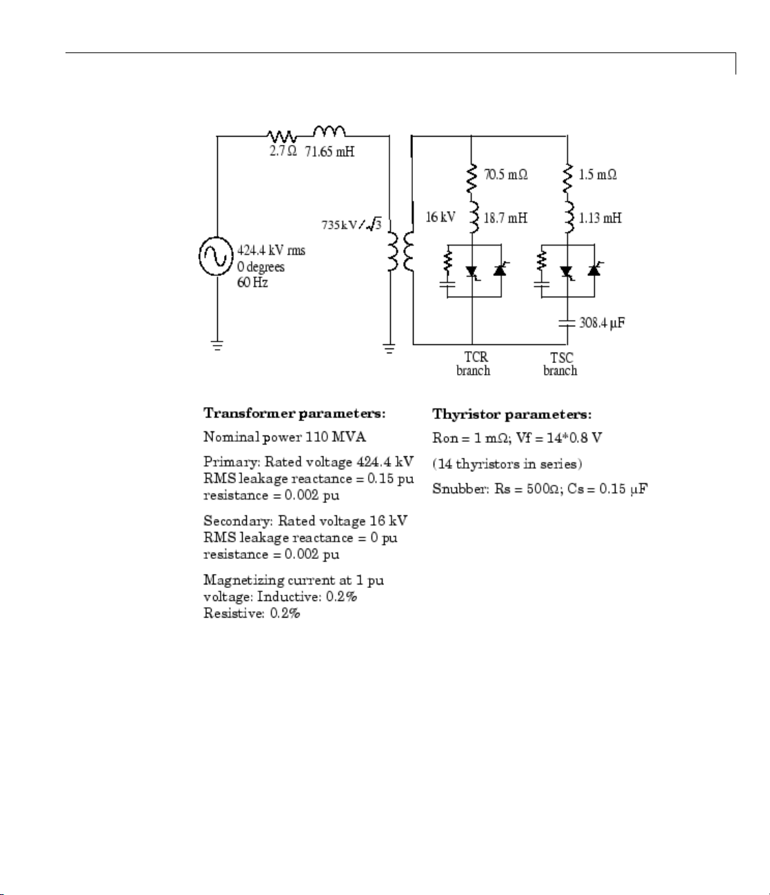
Introducing Power Electronics

One Phase of a TCR/TSC Static Var Compensator

The TCR and TSC branches are both controlled by a valve consisting of two thyristor strings con nected in antiparall el . An RC snubber circuit is connected across each valve. The TSC branch is switched on/off, thus providing discrete step variation of the SVC capacitive current. The TCR branch is phase controlled to obtain a continuous variation of the net SVC reactive current.

Now build two circuits illustrating the operation of the TCR and the TSC branches.

2-3

2 Advanced Components and Techniques

Simulation of the TCR Branch

1 Open a new window and save it as circuit3.

2 Open the Pow er Electronics library and copy the Thy risto r block into your

circuit3 model.

3 Double-click the block to open the Thyristor dialog box and set the

parameters as follows:

Ron

Lon

1e-3

14*0.8

500

0.15e-6

Notice that the snubber circuit is integral to the Thyristor dialog box.

4 Rename this block Th1 and duplicate it.

5 Connect this new thyristor Th2 in antiparallel with Th1, a s shown in

Simulation of the TCR Branch on page 2-6.

As the snubber circuit has already been specified with Th1, the snubber of Th2 m ust be eliminated.

6 Open the Th2 dialog box and set the snubber parameters to

Inf

2-4

Notice that the snubber disappears on the Th2 icon.

7 The Linear Transformer block is locat e d in the Elements library. Copy it,

rename it to TrA, and open its dialog box. Set its nominal power, frequency, and winding parameters ( winding 1 =

primary; winding 2 = secondary)

as shown in One Phase o f a TCR/TSC Static Var Compensator on page 2-3.

Introducing Power Electronics

The Units parameter allows you to specify the resistance R and leakage inductance L of each winding as well as the magnetizing branch Rm/Lm, either in SI units (ohms, henries) or in per units (pu). Keep the default pu setting to specify directly R and L in per unit quantities. As there is no tertiary winding, deselect Three windings transformer.Winding3 disappears on the TrA block.

Finally, set the magnetizing branch parameters Rm and Xm at

. These values correspond to 0.2% resistive and inductive currents.

500]

[500,

For more information on the per unit (pu) system, see “Per Unit”.

8 Add a voltage source, a Ground block, and a Series RLC Branch Block.

Set its parameters to

Branch type

Resistance

Inductance

9 Add a current measurement to measure the primary current. Interconnect

70.5e-3

18.7e-3

the circuit as shown in Simulation of the TCR Branch on page 2-6.

10 Notice that the Thyristor blocks have an output identified by the letter m.

This output returns a Simulink vectorized signal containing the thyristor current (Iak) and voltage (Vak). Connect a Demux block with two outputs at the m output of Th1. Then connect the two demultiplexer outputs to a dual trace scope that you rename Scope_Th1. (To create a second input to your scope, in the Scope properties > General menu item, set the number of axes to

2.) Label the two connection lines Ith1 and Vth1.These

labels are automatically displayed on the top of each trace.

2-5

2 Advanced Components and Techniques

Simulation of the TCR Branch

11 You can now model the synchronized pulse generators firing thyristors Th1

and Th2. Copy two Simulink pulse generators into your system, name them Pulse1 and Pulse2, and connect them to the gates of Th1 and Th2.

2-6

12 Now you have to define the timing of the Th1 and Th2 pulses. At every

cycle a pulse has to be sent to each thyristor α degrees after the zero crossing of the thyristor commutation voltage. Set the Pulse1 and Pulse2 block parameters as follows:

Amplitude

Period

Pulse width (% of period)

Phase Delay

13 The pulses sent to Th2 are delayed by 180 degrees with re spe ct to pulses

1/60 s

1% (3.6 degrees pulses)

1/60+T for Pulse1 1/60+1/120+T for Pulse2

sent to Th1. The delay T is used to specify the firing angle α.Togeta120 degree firing angle, specify

T = 1/60/3;

T in the workspace by entering

Introducing Power Electronics

14 Now open the Simulation > Configuration Parameters dialog box.

Select the set the relative tolerance to

15 Add a Powergui block at the top level of your model, then start the

ode23tb integration algorithm. Keep the default parameters but

1e-4 and the stop time to 0.1.

simulation. The results are shown in TCR Simulation Results on page 2-7.

Note You could also choose to discretize your system. Try, for example, asampletimeof50µs. Thesimulationresultsshouldcomparewellwith the continuous system.

Simulation Results

TCR

2-7

2 Advanced Components and Techniques

Simulation of the TSC Branch

You can now modify your circuit3 system and change the TCR branch to a TSC branch.

1 Save circuit3 a s a new system and nam e it circuit4.

2 Connect a capacitor of 308e-6 Farad in series with the RL inductor and

Th1/Th2 valve as shown in the fo llow ing figure, Simulation of the TSC Branch on page 2-9. Ch an g e the param e t ers of the RL block to

Resistance

Inductance

3 Connect a voltmeter and scope to monitor the voltage across the capacitor.

4 Contrary to the TCR branch, which was fired by a synchronous pulse

generator, a continuous firing signal is now applied to the two thyristors. Delete the two pulse generators. Copy a Step block from the Simulink library and connect its output at both gates of Th1 and Th2. Set its step time at 1/60/4 (energizing at the first positive peak of the source voltage). Your circuit should now be similar to the o ne shown here.

1.5e-3

1.13e-3

2-8

Introducing Power Electronics

Simulation of the TSC Branch

5 Open the three scopes and start the simulation.

As the capacitor is energized from zero, you can observe a low damping transient at 200 Hz, superimposed with the 60 Hz component in the capacitor voltage and primary current. During normal TSC operation, the capacitor has an initial voltage left since the last valve opening. To minimize the closing transient with a charged capacitor, the thyristors of the TSC branch must be fired when the source voltage is at maximum value and with the correct polarity. The initial capacitor voltage corresponds to the steady-state voltage obtained when the thyristor switch is closed. The capacitor voltage is 17.67 kVrms when the valve is conducting. At the closing time, the capacitor must be charged at the peak voltage.

=×=17670 2 24989

6 You can now use the Powergui block to change the capacitor initial voltage.

Open the Powergui and select Initial States Setting.Alistofallthe state variables with their default initial values appears. The value of the initial voltage across the capacitor C (variable

Uc_C) should be -0.314 1 V.

2-9

2 Advanced Components and Techniques

This voltage is not exactly zero because the snubber allows circulation of a small current when both thyristors are blocked. Now select the variable and enter button to make this change effective.

7 Start the simulation. As expected the transient component of capacitor

voltage and current has disappeared. The voltages obtained with and without initial voltage a re compared in this plot.

Uc_C state

24989 in the upper right field. Then click the Apply

2-10

Transient Capacitor Voltage With and Without Initial Charge

Simulating Variable Speed Motor Control

In this section...

“Introduction” on page 2-11 “Building and Simulating the PWM Motor Drive” on page 2-13 “Using the Multimeter Block” on page 2-19 “Discretizing the PWM Motor Drive” o n page 2-21 “Performing Harmonic Analysis Using the FFT Tool” on page 2-21

Introduction

In this section you

• Use electrical machines and power electronics to simulate a simple AC motor drive with variable speed control

• Learn how to use the Universal Bridg e block

Simulating Variable Speed Motor Control

• Discretize your model and compare variable-step and fixed-step simulation methods

• Learn how to use the Multimeter block

• Learn how to use the FFT tool

Variable speed control o f AC electrical machines makes use of forced-commutated electronic switches such as IGBTs, MOSFETs, and GTOs. Asynchronous machines fed by pulse width modulation (PWM) voltage sourced converters (VSC) are n owadays gradually replacing the DC motors and thyristor bridges. With PWM, combined with modern control techniques such as field-oriented control or direct torque control, you can obtain the same flexibility in speed and torque control as with DC machines. This section shows how to build a simple open loop AC drive controlling an asynchronous machine. Chapter 4 will introduce you to a specialized library containing 13 models of DC and AC drives. These “ready to use” models will enable you to simulate electric drive systems without the need to build those complex systems yourself.

2-11

2 Advanced Components and Techniques

The Machines library contains four of the most commonly used three-phase machines: simplified and complete synchronous machines, asynchronous machine, and p ermanent magnet synchronous machine. Each machine can be used either in generator or motor mode. Combined with linear and nonlinear elements such as transformers, lines, loads, breakers, etc., they can be used to simulate electromechanical transients in an electrical network. They can also be combined with power electronic devices to simulate drives.

The Power Electronics library contains blocks allowing you to simulate diodes, thyristors, GTO thyristors, MOSFETs, and IGBT devices. You could interconnect several blocks together to build a three-phase bridge. For examp le , an IGBT inverter bridge would require six IGBTs and six antiparallel diodes.

To facilitate implementation of bridges, the Universal Bridge block automatically performs these interconnections for you.

Circuit 5: PWM Control of an Induction Motor

2-12

Simulating Variable Speed Motor Control

Building and Sim

Follow these ste

ps to build a PWM -controlled motor.

ulating the PWM Motor Drive

Assembling and Configuring the Motor Blocks

In the first st

1 Open a new wind

2 Open the Power Electronics library and copy the U niv ersal Bridge block

into your

3 Open the Universal Bridge dialog box and set its parameters as follows:

Power electronic device

Snubber

Forward voltages

eps, you copy and set up the motor blocks:

ow and save it as

circuit5 model.

Ron

Vfd

circuit5.

IGBT/Diode

1e5 Ω

inf

1e-3 Ω

Tail

1e-

-6 s

Notice that the snubber circuit is integral to the Universal Bridge dialog box. As the Cs capacitor value of the snubber is set to

Inf (short-circuit), we

are using a purely resistive snubber. Generally, IGBT bridges do not use snubbers; however, because each nonlinear element in SimPowerSystems software is modeled as a current source, you have to provide a parallel path across each IGBT to allow connection to an inductive circuit (stator of the asynchronous machine). The high resistance value of the snubber does not affect the circuit performance.

2-13

2 Advanced Components and Techniques

4 Open the Machines library. Copy the Asynchronous Machine SI Units block

as well as the M achine Measurement Demux block into your model.

5 Open the Asynchronous Machine menu and look at its parameters. Set the

nominal power Pn parameter to 3*746 VA and the nominal line-to-line voltage Vn to 220 Vrms to implement a 3 HP, 60 Hz machine with two pairs of poles. Its nominal speed is therefore slightly lower th an the synchronous speed of 1800 rpm, or w

6 Notice that the three rotor terminals a,b,andc are made accessible.

During normal motor operation these terminals should be short-circuited together. In the Asynchronous Machine menu change the rotor type to Squirrel cage. Notice that after this change the rotor connections are no longer accessible.

7 Open the Machine Measurement Demux block menu. When this block is

connected to a machine measurement output, it allows you to access specific internal signals of the machine. First select the Asynchronous machine type. Deselect all signals except the following three signals: stator currents),

circuit5

= 188.5 rad/s.

is_abc (three

wm (rotor speed), and Te (electromagnetic torque).

2-14

Loading and Driving the Motor

You n ow implement the torque-spe ed characteristic of the motor load. Assume a quadratic torque-speed characteristic (fan or pump type load). The torque T is then proportional to the square of the speed ω.



×=3 746

188 5

11 87

188 5

11 87..

334 10

−

Tk=×

The nominal torque of the m otor is

TNm

Therefore, the constant k should be

== = ×

Simulating Variable Speed Motor Control

1 Open the User-Defined Functions library of Simulink and copy the Fcn

block into your expression of torque as a function of speed:

2 Connect the input of the Fcn block to the speed output of the Machines

Measurement Demux block, labeled of the motor, labeled

3 Open the Electrical Sources library and copy the DC Voltage Source block

into your

circuit5 model. Open the block menu and enter the

3.34e-4*u^2.

wm, and its output to the torque input

Tm.

circuit5 model. Open the block menu and set the v oltage to

400 V.

4 Open the Measurements library and copy a Voltage Measurement block

into your

5 Using Ground blocks from the Elements library, complete the power

circuit5 model. Change the block name to Vab.

elements and voltage sensor interconnections as shown in Circuit 5: PWM Control of an Induction Motor on page 2-12.

Controlling the Inverter Bridge with a Pulse Generator

To control your inverter bridge, you need a pulse generator. Such a generator is available in the Extras library of powerlib:

1 Open the Extras/Discrete Control blocks library and copy the Discrete

3-Phase PWM Generator block into your can be used to generate pulses for a t w o-lev el or a three-level bridge. In addition the block generates two sets of pulses (outputs P1 and P2) that can be sent to two different three-arm bridges when the converter uses a twin bridge configur a t ion . In this case, use it as a two-level single-bridge PWM generator. The converter operates in an open loop, and the three PWM modulating signals are generated internally. Connect the P1 output to the pulses input of the Universal Bridge block

2 Open the D iscrete Three-Phase PW M Generator block dialog box and set

the parameters as follows.

Type

Mode of operation

Carrier frequency

circuit5 model. This block

2 level

Un-synchronized

18*60Hz (1080 Hz)

2-15

2 Advanced Components and Techniques

Internal generation of modulating

selected

signals

Modulation index m

Output voltage frequency

Output voltage phase

Sample time

3 Use the Edit > Look Under Mask menu item of your model window to see

0.9

60 Hz

0 degrees

10e-6 s

how the PWM is implemented. This control system is made entirely with Simulink blocks. The block has been discretized so that the pulses change at multiples of the sp ecif ied time step. A time step of 10 µs corresp onds to +/- 0.54% of the switching period at 1080 Hz.

One common method of generating the PWM pulses uses comparison of the output voltage to synthesize (60 Hz in this case) with a triangular wave at the switching frequency (1080 Hz in this case). This is the method that is implemented in the Discrete 3-Phase PWM Generator block. The line-to-line RMS output voltage is a function of the DC input voltage and of the modulation index m as given by the following equation:

LLrms

=× =× ×

Vdc m VDC

0 612.

2-16

Therefore, a DC voltage of 400 V and a modulation facto r of 0.90 yield the 220 Vrms output line-to-line v oltag e, which is the nominal voltage of the asynchronous motor.

Displaying Signals and Measuring Fundamental Voltage and Current

1 You now add blocks measuring the fundamental component (60 Hz)

embedded in the chopped Vab voltage and in the phase A current. Open the Extras/Discrete Measurements library of powerlib and copy the dis crete Fourier block into your

circuit5 model.

Simulating Variable Speed Motor Control

Open the discrete Fourier block dialog box and check that the parameters are set as follows:

Fundamental frequency f1

Harmonic number

Initial input

Sample time

60 Hz

[0 0]

10e-6 s

Connect this block to the output of the Vab voltage sensor.

2 Duplicate the Discrete Fourier block. To measure the phase A current,

you need to select the first element of the

is_abc output of the ASM

Measurement Demux block.

Copy a Selector block from the Signals & Systems Simulink library.

Open its menu and set Element to second Discrete Fourier block and its input to the

1. Connect the Selector output to the is_abc output of the

Machines Measurement Demux block as shown in Circuit 5: PWM Control of an Induction Motor on page 2-12.

3 Finally, add scopes to your model. Copy one Scope block into your circuit.

This scope is use d to display the instantaneous motor voltage, currents, speed, and electromagnetic torque. In the Scope properties > General menu of the scope, set the following parameters:

Number of axes

Time range

Tick labels

0.05 s

bottom axis only

Connect the four inputs and label the four connection lines as shown in TCR Simulation Results on page 2-7. When you start the simulation, these labels are displayed on top of each trace.

To allow further processing of the signals displayed on the oscilloscope, you have to store them in a variable. In the Scope properties > Data

history menu of the scope, set the following parameters:

2-17

2 Advanced Components and Techniques

Limit data point to last

Save data to worksp ace

variable name

Format

After simulation, the four signals displayed on the scope are available in a structure array named ASM.

4 Duplicate the four-input Scope and change its number of inputs to 2. This

scopeisusedtodisplaythefundamental component of Vab voltage and Ia current. Connect the two inputs to the outputs of the Fourier blocks. Label the two connection lines as shown in TCR Simulation Results on page 2-7.

You are n ow ready to simulate the mot or starting.

deselected

selected

ASM

Structure with time

Simulating the PWM Motor Drive with Continuous Integration Algorithm

Open the Simulation > Configuration Parameters dialog box. S elect the

ode23tb integration algorithm. Set the relative tolerance to 1e-4,the

absolute tolerance and the Max step size to Start the simulation. The sim ulation results are shown in PWM Motor Drive ; Simulation Results for Motor Starting at Full Voltage on pag e 2-19.

auto, and the stop time to 1s.

2-18

The motor starts and r eaches its steady-state speed of 181 rad/s (1728 rpm) after 0.5 s. At starting, the magnitude of the 60 Hz current reaches 90 A peak (64 A RMS) whereas its steady-state value is 10.5 A (7.4 A RMS). As expected, the magnitude of the 60 Hz voltage contained in the chopped w ave stays at

220 2 311×= V

Also notice strong oscillations of the electromagnetic torque at starting. If you zoom in on the torque in steady state, you should observ e a noisy signal with a mean value of 11.9 N.m, corresponding to the load torque at nominal speed.

If you zoom in on the three motor currents, you can see that all the harmonics (multiples of the 1080 Hz switching frequency) are filtered by the stator inductance, so that the 60 Hz component is dominant.

Simulating Variable Speed Motor Control

PWM Motor Drive; Simulation Results for Motor Starting at Full Voltage

Using the Multimeter Block

The Universal Bridge block is not a conventional subsystem where all the six individual switches are accessible. If you want to measure the switch voltages and currents, you must use the Multimeter block, which gives access to the bridge internal signals:

1 Open the Universal Bridge dialog box and set the Measurement

parameter to

y the Multimeter block from the Measurements library into your

2 Cop

cuit5

cir

six switch currents appears.

the

Device currents.

circuit. Double-click the Multimeter block. A window showing

2-19

2 Advanced Components and Techniques

3 Select the two currents of the bridge arm connected to phase A. They are

identified as

iSw1

iSw2

4 Click OK. The number of signals (2) is displayed in the multimeter icon.

5 UsingaDemuxblock,sendthetwomultimeter output signals to a two-trace

scope and label the two connection lines (Trace 1:

6 Restart the simulation. The waveforms obtained for the first 20 ms are

Universal Bridge

iSw1 Trace 2: iSw2).

showninthisplot.

2-20

Currents in IGBT/Diode Switches 1 and 2

As expected, the currents in switches 1 and 2 are complementary. A positive current indicates a current flowing in the IGBT, whereas a n egative current indicates a current in the an t iparallel diode.

Simulating Variable Speed Motor Control

Note Multimeter block use is not limited to the Universal Bridge block. Many blocks of the Electrical Sources and Elements libraries have a Measurement parameter where you can select voltages, currents, or saturable transformer fluxes. A judicious use of the Multimeter block reduces the number of current and voltage sensors in your circu it, making it easier to follow.

Discretizing the PWM Motor Drive

You might have noticed that the simulation using a variable-step integration algorithm is relatively long. Depending on your computer, it might take tens of seconds to simulate one second. To shorten the simulation time, you can discretize your circuit and simulate at fixed simulation time steps.

Open the Powergui, click Configure Parameters, and in the Powergui block parameters dialog box set Simulation type to Sample time to including the asynchronous machine, is discretized at a 10 µs sample time.

10e-6 s. When you restart the simulation, the power system,

Discrete.Setthe

As there are no more continuous states in the electrical system, you do notneedavariable-stepintegrationmethod to solve this system. In the Simulation > Configuration Parameters > Solver dialog box pane, select the

Fixed-step and Discrete (no continuous states) options.

Start the simulation. Observe that the simulation is now approximately three times faster than with the continuoussystem. Resultscomparewell with the continuous system.

Performing Harmonic Analysis Using the FFT Tool

The two Discrete Fourier b locks allow computation of the fundamental component of voltage and current while simulation is running. If you would like to observe harmonic components alsoyouwouldneedaDiscreteFourier block for each harmonic. This approach i s not conve nient.

Now use the FFT tool of Powergui to display the frequency spectrum of voltage and current waveforms. These signals are stored in your workspace in the ASM structure with time variable generated by the Scope block. Because

2-21

2 Advanced Components and Techniques

your model is discretized, the signal saved in this structure is sampled at a fixed step and consequently satisfies the FFT tool requirements.

Open the Powergui and select FFT Analysis. A new window opens. Set the parameters specifying the analyzed signal, the time window, and the frequency range as follows:

Structure

Input

Signal number

Start time

Number of cycles

(pull-down menu)

Fundamental frequency

Max Frequency

Frequency axis

Display style

ASM

Vab

0.7 s

Display FFT window

60 Hz

5000 Hz

Harmonic order

Bar (relative to Fund or DC)

The analyzed signal is displayed in the upper w indow. Click Display.The frequency spectrum is displayed in the bottom window, as shown in the next figure.

2-22

Simulating Variable Speed Motor Control

FFT Analysis of the Motor Line-to-Line Voltage

The fundamental component and total harmonic distortion (THD)ofthe Vab voltage are displayed above the spectrum window. The magnitude of the fundamental of the inverter voltage (312 V) compares well with the theoretical value (311 V for m=0.9).

Harmonics are displayed in percent of the fundamental component. A s expected, harmonics occur around multiples of carrier frequency (n*18 +- k).

2-23

2 Advanced Components and Techniques

Highest harmonics (30%) appear a t 16th h armonic (18 - 2) and 20th harmonic (18 + 2).

Finally, select input Ia instead of Vab and display its current spectrum.

2-24

Three-Phase Systems and Machines

In this section...

“Introduction” on page 2-25 “Three-Phase Network with Electrical Machines” on page 2 -25 “Load Flow and Machine Initialization” on page 2-28 “Using the Phasor Solution Method for Stability Studies” on page 2-36

Introduction

In this section you

• Learn how to simulate a three-phase power system containing electrical machines and other three-phase models

• Perform a load flow study and initialize machines to start simulation in steady state by using the Load Flow and Machine Initialization option of the Powergui

Three-Phase Systems and Machines

• Simulate the power system and observe its dynam ic performance by using both the standard solution technique using a continuous solver and the phasor simulation method

You now use three types of machines of the Electrical Machines library: simplified synchronous machine, detailed synchronous machine, and asynchronous machine. You interconnect these machines with linear and nonlinear elements such as transformers, loads, and breakers to study the transient stability of an uninterruptible power supply using a diesel generator.

Three-Phase Network with Electrical Machines

The two-machine system shown in this single line dia gram is this section’s main example:

2-25

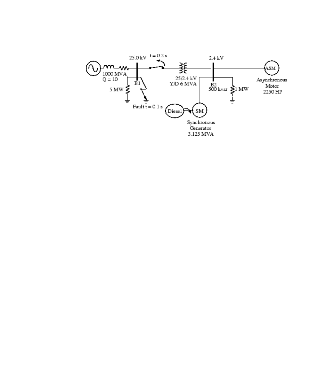
2 Advanced Components and Techniques

DieselGeneratorandAsynchronousMotoronDistributionNetwork

This system consists of a plant (bus B2), simulated by a 1 MW resistive load andamotorload(ASM)fedat2400Vfromadistribution25kVnetwork through a 6 MVA, 25/2.4 kV transformer, and from an emergency synchronous generator/diesel engine unit (SM).

2-26

The 25 kV network is modeled by a simple R-L equivalent source (short-circuit level 1000 MVA, quality factor X/R = 10) and a 5 MW load. The asynchronous motor is rated 2250 HP, 2.4 kV, and the synchronous machine is rated 3.125 MVA, 2.4 kV.

Initially, the motor develops a mechanical power of 2000 HP and the diesel generator is in standby, delivering no active power. The synchronous machine therefore operates as a synchrono us condenser g enerating only the reactive power required to regulate the 2400 V bus B2 voltage at 1.0 pu. At t = 0.1 s, a three-phase to ground fault occurs on the 25 kV system, causing the opening of the 25 kV circuit breaker at t = 0.2 s, and a s udden increase of the generator loading. During the transient period following the fault and islanding of the motor-generator system, the synchronous machine excitation system and the diesel speed governor react to maintain the voltage and speed at a constant value.

This system is modeled in the illustration.

power_machines demo, shown in the following

Three-Phase Systems and Machines

Power System of Diesel Generator and Asynchronous Motor on Distribution Network

The Synchronous Machine (SM) block uses standard parameters, whereas the Asynchronous Machine (ASM) block uses SI parameters.

The other three-phase elements such as the inductive voltage source, the Y grounded/Delta transformer, and the loads are standard blocks from the Electrical Source and Elements libraries of powerlib. If you open the dialog box of the Three-Phase Fault and Three-Phase Breaker blocks, you see how the switching times are specified. The M achine Measurement Demux block provided in the Machines library is used to demux the output signals of the SM and ASM machines.

The SM voltage and speed outputs are used as feedback inputs to a Simulink control system that contains the diesel engine and g ov ernor block as well as an excitation block. The excitation system is the standard block provided in the Machines library. The SM parameters as well as the diesel engine and governor models were taken from reference [1].

2-27

2 Advanced Components and Techniques

Diesel Engine and Governor System

If you simulate this system for the first time, you normally do not know what the initial conditions are for the SM and ASM to start in steady state.

These initial conditions are

• SM block: Initial values of speed deviation (usually 0%), rotor angle, magnitudes and phases of currents in stator windings, and initial field voltage required to obtain the desired terminal voltage under the specified load flow

2-28

• ASM block: Initial values of slip, rotor angle, magnitudes and phases of currents in stator windings

Open the dialog box of the Synchronous Machine and Asynchronous Machine blocks. All initial conditions should b e set at fieldvoltageandASMslip,whicharesetat monitoring the SM and ASM signals as well as the bus B2 voltage. Start the simulation and observe the first 100 ms before fault is applied.

As the simulation starts, note that the three ASM currents start from zero and contain a slowly decaying DC component. The machine speeds take a much longer time to stabilize because of the inertia of the motor/load and diesel/generator systems. In our example,theASMevenstartstorotatein the wrong direction because the motor starting torque is lower than the applied load torque. Stop the simulation.

0, except for the initial SM

1pu. Open the three scopes

Load Flow and Machine Initialization

To start the simulation in steady state with sinusoidal currents and constant speeds, all the machi n e states must be init ialized properly. This is a d if ficult task to perform manually, ev en for a simple system. In the next section you

Three-Phase Systems and Machines

learn how to use the Load Flow and Machine Initialization option of the Powergui block to perform a load flow and initialize the machines.

Double-click the Pow ergui block and click the Load Flow an d Machine Initialization button. A new window appears. In the upper right window you have a list of the machines appearing in your system. Select the SM 3.125 MVA machine. Note that for the Bus Type, you have a menu allowing you to choose either PV Generator, PQ Generator, or Swing G enerator.

For synchronous machines you normally specify the desired term in a l voltage and the active power that you want to generate (positive p ow er for generator mode)orabsorb(negativepowerformotormode). Thisispossibleaslongas you have a swing (or slack) bus that generates or absorbs the excess po we r required to balance the active powers throughout the network.

The swing bus can be either a voltage source or any other synchronous machine. If you do not have any voltage source in your system, you must declare one of the machines as a swing machine. In the next section, you perform a load flow with the 25 kV voltage source connected to bus B1, which is used as a swing bus.

Load Flow Without a Swing Machine

In the Load Flow window, your SM Bus Type should a lread y be initialized as

P & V generator, in d icating that the load flow is performed with the

machine controlling its active power and terminal voltag e. By default, the desired Terminal Voltage UAB is initialized at the nominal machine voltage (2400 Vrms). Keep it unchanged and set the Active Power to zero. The synchronous machine therefore absorbs or generates reactive power only to keep terminal voltage at 1 pu. Now select the ASM 2250 HP machine in the upper right window. The only parameter that is needed is the Mechanical

power developed by the motor. Enter 2000*746 (2000 HP) and click the Update Circuit & Measurements button. You now perform the load flow

with the f ollowing parameters.

Terminal Voltage

Active Power

2400 Vrms

0kW

2-29

2 Advanced Components and Techniques

ASM

Click the Update Load Flow button. Once the load flow is solved, the three phasors of line-to-line machine voltages as well as currents are updated as shownonthenextfigure.ValuesaredisplayedbothinSIunits(voltsRMS or amperes RMS) and in pu.

Mechanical Power

2000*746 W (2000 HP)

2-30

The SM active and reactive powers, mechanical power, and field voltage are displayed.

P0W

Q85

6 kvar

or 856/3125 = 0.2739 pu

Three-Phase Systems and Machines

Pmec

844.2 W

or 0.00027 pu, representing

internal machine losses in stator windings

Ef (field voltage) 1.427 pu

The ASM active and reactive powers absorbed by the motor, slip, and torque are also displayed.

P 1.515 MW (0.9024 pu)

Q 615 kvar (0.3662 pu)

Pmec 1.492 MW (2000 HP)

Slip 0.006119

Torque 7964 N.m (0.8944 pu)

Close t

The ASM block ASM di the lo You c of th of th

Faul

pha

he Load Flow window.

torque value (7964 N.m) should already be entered in the Constant

connected at the ASM torque input. If you now open the SM and

alog boxes you can see the updated initial conditions. If you open ad flow tool, you can see updated values of the measurement outputs. an also click the Nonlinear button to obtain voltages and currents

e nonlinear blocks. For example, you should find that the magnitude

e Phase A voltage across the fault breaker (named

t/Breaker1

) is 14.42 kV RMS, corresponding to a 24.98 kV RMS

Uc_3-Phase

se-to-phase voltage.

tart the simulation in steady state, the states of the Governor & D iesel

To s

ine and the Excitation blocks should also be initialized according to the

Eng

lues calculated by the load flow. Open the Governor & Diesel Engine

bsystem, which is inside the Diesel Engine Speed and Voltage Control

bsystem. Notice that the initial mechanical power has been automatically

tto

0.0002701 pu. Open the Excitation block and notice that the initial

erminal voltage and field voltage have been set respectively to

.427 pu

1.0 and

2-31

2 Advanced Components and Techniques

Note that t he load flow also initializes the Constant blocks connected at the reference inputs (wref and v ref) of the Governor and Excitation blocks as well as the Constant block connected at the load torque input (Tm) of the Asynchronous Machine block.

Open the three scopes displaying the internal signals of synchronous and asynchronous machines and phase A voltage. Start the simulation. The simulation results are shown in the following figure.

2-32

Simulation Results

Observe that during the fault, the terminal voltage drops to about 0.2 pu, and the excitation voltage hits the limit of 6 pu. After fault clearing and islanding, the SM m echanical power quickly increases from its initial value of 0 pu

Three-Phase Systems and Machines

to 1 pu an d stabilizes at the final value of 0.82 pu required by the resistive and motor lo ad (1.0 MW resistive lo ad + 1.51 MW motor load = 2.51 MW =

2.51/3.125 = 0.80 pu). After 3 seconds the terminal voltage stabilizes close to its reference value of 1.0 pu. The motor speed temporarily decreases from 1789 rpm to 1635 rpm, then recovers close to its normal value after 2 seconds.

If you increase the fault duration to 12 cycles by changing the breaker opening time to 0.3 s, notice that the system collapses. The ASM speed slows down to zero after 2 seconds.

Load Flow with a Swing Machine

In this section y ou make a load flow with two synchronous machine types: a PV generator and a swing generator.Inyourpower_machines window, delete the inductive source and replace it with the Simplified Synchronous Machine block in pu from the Machines library. Rename this machine SSM 1000MVA. Add two constant blocks at the Pm and E inputs of the Simplified Synchronous Machine. These two blocks, which are used to specify the mechanical power and the machine internal voltage, will be autom a tica lly initialized when you perform a new load flow. Save this new system in your working directory as box and enter the following parameters:

power_machines2.mdl.Open the SSM 1000 MVA dialog

Connection type

Pn(VA), Vn(Vrms),

3-wire Y

[1000e6 25e3 60]

fn(Hz) H(s), Kd(), p (),

R(pu), X(pu)

Init. cond.

[inf 0 2]

[0.1 1. 0]

Leave all initial conditions at zero.

As you specify an infinite inertia, the speed and therefore the frequency of the machine are kept constant. Notice how easily you can specify an inductive short-circuit level of 1000 MVA and a quality factor of 10 with the per unit system.

Also, connect at inputs 1 and 2 of the SSM block two Constant blocks specifying respectively the required mechanical power (Pmec) and its internal

2-33

2 Advanced Components and Techniques

voltage (E). These two constants are updated automatically according to the load flow solution.

When there is no voltage source imposi ng a reference ang le for voltages, you must choose one of the synchronous machines as a reference. In a load flow program, this reference is called the swing bus. The swing bus absorbs or generates the power neededtobalancetheactivepowergeneratedbytheother machines and the power dissip ated in loads as well as losses in all elemen ts.

Open the Powergui. In the Tools menu, select Load Flow and Machine Initialization. Change the SSM Bus Type to load flow by entering the following parameters for the SM and ASM machines:

SM 1000 MVA:

Terminal voltage UAB

Active power

ASM 2250 HP:

Mechanical power

Swing Generator.Specifythe

2400 Vrms

1.492e+06 W (2000 HP)

2-34

For the SSM swing machine you only have to specify the requested terminal voltage (magnitude and phase). The active power is unknow n . How ev er, you canspecifyanactivepowerthatisusedasaninitialguessandhelploadflow convergence. Respecify the following SSM param eters:

Terminal voltag e

24984 Vrms

(this voltage obtained at bus B1 from the previous load flow)

Phase of UAN voltage

Active power guess

0 degrees

7.5e6 W

(estimated power = 6 MW (resistive load) + 1.5 MW motor load)

Three-Phase Systems and Machines

Click the Update Load Flow button. Once the load flow is s olved the following solution is displayed. Use the scroll bar of the left window to look at the solution for each of the three machines.

The active and reactive electrical powers, mechanical power, and internal voltage are displayed for the SSM block.

.542 MW; Q=-147 kvar

P=7

ec=7.547 MW (or 7.547/1000=0.007547 pu)

ternal voltage E=1.0 pu

2-35

2 Advanced Components and Techniques

The active and reactive electrical powers, mechanical power, and field voltage of the SM block are

P=0 W; Q=856 kvar Pmec=844 W Vf=1.428 pu

The active and reactive powers absorbed by the motor, slip, and torque of the ASM block are also displayed.

P=1.515MW Q=615 kvar Pmec=1.492 MW (2000 HP) Slip=0.006119 Torque=7964 N.m

As expected, the solution obtained is exactly the same as the one obtained with the R-L voltage source. T he active power delivered by the swing bus is 7.54 MW (6.0 MW resistive load + 1.51 MW motor load = 7.51 MW, the difference (0.03 MW) corresponding to losses in the trans former).

Restart the simulation. You should get the same waveforms as those show n in the figure called Simulation Results o n page 2-32.

2-36

Reference

[1] Yeager, K.E., and J.R.Willis, “Modeling of Emergency Diesel Generators in an 800 Megawatt Nuclear Power Plant,” IEEE

Conversion, Vol. 8, No. 3, September, 1993.

Transactions on Energy

Using the Phasor Solution Method for Stability Studies

Up to now, you have simulated a relatively simple power system consisting of a maximum of three machines. If you increase complexity of your network by adding extra lines, loads, transformers, and machines, the required simulation time becomes longer and longer. Moreover, if you are interested in slow electromechanical oscillation modes (typically between 0.02 Hz and 2 Hzonlargesystems)youmighthavetosimulateforseveraltensofseconds, implying simulation times of minutes and even hours. The conventional continuous or discrete solution method is therefore not practical for stability studies involving low-frequency oscillation modes. To allow such studies, you

Three-Phase Systems and Machines

have to use the phasor technique (see “Introducing the Phasor Simulation Method” on page 1-40).

For a stability study, we are not interested in the fast oscillation modes resulting from the interaction of l inear R, L, C elements and distributed parameter lines. These oscillation modes, which are usually located above the fundamental frequency of 50 H z or 60 H z, do not interfere with the slow machine modes and regulator time constants. In the phasor solution method, these fast modes are ignored by replacing the network’s differential equations by a set of algebraic equations. The state-space model of the network is therefore replaced by a transfer function evaluated at the fundamental frequency and relating inputs (current injected by machines into the network) and outputs (voltages at machine terminals). The phasor solution method uses a reduced state-space model consisting of slow states of machines, turbines, and regulators, thus dramatically reducing the required simulation time. Continuous variable-step solvers are very efficient in solving this type of problem. Recommended solver is

ode23tb with a maximum time step of

one cycle of the fundamental frequency (1/60 s or 1/50 s).

Now apply the phasor solution method to the two-machine system you have just simulated with the conventional method. Open the

power_machines

demo.

Double-click the Powergui, click Configure Parameters,andinthe Powergui block parameters dialog box set Simulation type to

Phasor.You

must also specify the fundamental frequency used to solve the algebraic network equations. A default value of 60 Hz should already be entered in the Phasor frequency field. Close the Powergui and notice that the word

Phasors now appears on the Powergui icon, indicating that this new method

canbeusedtosimulateyourcircuit.Tostart the simulation in steady state, you must first repeat the load flow and machine initialization procedure explained in the previous section, “Load Flow and Machine Initialization” on page 2-28.

In the Configuration Parameters dialog box, specify a Max step size of

1/60 s (one cycle) and start the simulation.

Observe that simulation is now much faster. T he results compare well with those obtained in the previous simulation. A comparison of synchronous machine and asynchronous machine signals is shown b elow.

2-37

2 Advanced Components and Techniques

2-38

Comparison of Results for Continuous and Phasor Simulation Methods

The phasor solution method is illustrated on more complex networks presented as the following demos:

• Transient stability of two machines with power sys tem stabilizers (PSS) and a static var compensator (SVC) (

• Performance of three power system stabilizers for interarea oscillations (

power_PSS model)

power_svc_pss model)

Three-Phase Systems and Machines

The first demo illustrates the impact of PSS and use of a SVC to stabilize a two-machine system. The second demo compares the performance of three different types of power system stabilizers on a four-machine, two-area system.

The phasor solution method is also used for FACTS models available in the

factslib library. Three case studies demonstrating p h asor simulation are

presented in Chapter 6, “Transient Stability of Power Systems Using Phas or Simulation”.

2-39

2 Advanced Components and Techniques

Building and Customizing Nonlinear Models

In this section...

“Introduction” on page 2-40 “Modeling a Nonlinear Inductance” on page 2-40 “Customizing Your Nonlinear Model” on page 2 -45 “Modeling a Nonlinear Resistance” on page 2-48 “Creating Your Own Library” on page 2-53 “Connecting Your Model with Other Nonlinear Blocks” on page 2-53

Introduction

SimPowerSystems software provides a wide collection of nonlinear models. It can happen, however, that you need to interface your own nonlinear model with the standard models provided in the powerlib library. This model could be a simple nonlinear resistance simulating an arc or a varistor, a saturable inductor, a new type of motor, etc.

2-40

In the following section you learn how to build such a nonlinear m odel. A simple saturable inductance and a nonlinear resistance serve as examples.

Modeling a Nonlinear Inductance

Consider an inductor of 2 henries designed to operate at a nominal voltage, Vnom = 120 V RMS, and a nominal frequency, fnom = 60 Hz. From zero to 120 V RMS the inductor has a constant inductance, L = 2 H. W hen voltage exceeds its nominal voltage, the inductor saturates and its inductance is reduced to Lsat = 0.5 H. The nonlinear flux-current characteristic is plotted in the next figure. Flux and current scales are in per units. The nominal voltage and nominal current are chosen as base values for the per-unit system.

Building and Customizing Nonlinear Models

Flux-Curr

The curre that, in t are given

The model of the nonlinear inductance can therefore be implemented as a controlled current source, where current i is a nonlinear function of v oltage v,asshown.

Model of a Nonlinear Inductance

ent Characteristic of the Nonlinear Inductance

nt i flowing in the inductor is a nonlinear function of flux linkage ψ

urn, is a function of v appearing across its terminals. These relations

by the f ollowing equations:

didtd

=⋅ = = ⋅



()



vdt



∫

2-41

2 Advanced Components and Techniques

Implementation of a Nonlinear Inductance on page 2-42 shows a circuit using a 2 H nonlinear inductance. The nonlinear inductance is connected in series with two voltage sources (an AC Voltage Source block of 120 volts RMS, 60 Hz, and a DC Voltage Source block) and a 5 ohm resistor.

All the elements used to build the nonlinear model have been grouped in a subsystem named Nonlinear Inductance. The inductor terminals are labeled

In and Out. Notice that a second output returning the flux has been added to

the subsystem. You can use this output to observe the flux by connecting it to a Simulink Scope block.

The nonlinear model uses two powerlib blocks and two Simulink blocks. The two powerlib blocks are a Voltage Measurement block to read the voltage at the inductance terminals and a Controlled Current Source block. The direction of the arrow of the current source is oriented from input to output according to the model shown above.

The two Simulink blocks are an Integrator block computing the flux from the voltage input and a Look-Up Table block imp lementing the sa tu rati on characteristic i=f(ψ) described by Flux-Current Characteristic of the Nonlinear Inductance on page 2-41.

2-42

lementation of a Nonlinear Inductance

Imp

Mathworks SIMPOWERSYSTEMS 5 user guide

Specifications and Main Features

Frequently Asked Questions

User Manual

Acknowledgments

Getting Started

Product Overview

Introduction

TheRoleofSimulationinDesign

SimPowerSystems Libraries

Using This Guide

If You Are a New User

If You Are an Experienced Blockset User

All Users

Units

Building and Simulating a Simple Circuit

Introduction

Building the Electrical Circuit with powerlib Library

Interfacing the Electrical Circuit with Other Simulink Blocks

Measuring Voltages and Currents

Basic Principles of Connecting Capacitors and Inductors

Analyzing a Simple Circuit

Introduction

Electrical State Variables

Frequency Analysis

Specifying Initial Conditions

Introduction

State Variables

Initial States

Specify Initial Electrical States with Powergui

Forcing Initial States to Zero

Forcing Initial States to Steady State

Returning to Block Settings

Simulating Transients

Introduction

Simulating Transients with a Circuit Breaker

Continuous, Variable Time Step Integration Algorithms

Discretizing the Electrical System

Introducing the Phasor Simulation Method

Introduction

When to Use the Phasor Solution

Phasor Simulation of a Circuit Transient

Invoking the Phasor Solution in the Powergui Block

Selecting Phasor Signal Measurement Formats

Processing Voltage and Current Phasors

Advanced Components and Techniques

Introducing Power Electronics

Introduction

Simulation of the TCR Branch

Simulation of the TSC Branch

Simulating Variable Speed Motor Control

Introduction

Assembling and Configuring the Motor Blocks

Loading and Driving the Motor

Controlling the Inverter Bridge with a Pulse Generator

Displaying Signals and Measuring Fundamental Voltage and Current

Using the Multimeter Block

Discretizing the PWM Motor Drive

Performing Harmonic Analysis Using the FFT Tool

Three-Phase Systems and Machines

Introduction

Three-Phase Network with Electrical Machines

Load Flow and Machine Initialization

Load Flow Without a Swing Machine

Load Flow with a Swing Machine

Reference

Using the Phasor Solution Method for Stability Studies

Building and Customizing Nonlinear Models

Introduction

Modeling a Nonlinear Inductance