Mathworks SIMMECHANICS 3 user guide

Download

SimMechanics™ 3

User’s Guide

How to Contact The MathWorks

www.mathworks. comp.soft-sys.matlab Newsgroup www.mathworks.com/contact_TS.html Technical Support

suggest@mathworks.com Product enhancement suggestions

bugs@mathwo doc@mathworks.com Documentation error reports service@mathworks.com Order status, license renewals, passcodes

info@mathwo

com

rks.com

Web

Bug reports

Sales, prici

ng, and general information

508-647-7000 (Phone)

508-647-7001 (Fax)

The MathWorks, Inc. 3 Apple Hill Drive Natick, MA 01760-2098

For contact information about worldwide offices, see the MathWorks Web site.

SimMechanics™ User’s Guide

The software described in this document is furnished under a license agreement. The software may be used or copied only under the terms of the license agreement. No part of this manual may be photocopied or reproduced in any form without prior written consent from The MathW orks, Inc.

FEDERAL ACQUISITION: This provision applies to all acquisitions of the Program and Documentation by, for, or through the federal government of the United States. By accepting delivery of the Program or Documentation, the government hereby agrees that this software or documentation qualifies as commercial computer software or commercial computer software documentation as such terms are used or defined in FAR 12.212, DFARS Part 227.72, and DFARS 252.227-7014. Accordingly, the terms and conditions of this Agreement and only those rights specified in this Agreement, shall pertain to and govern theuse,modification,reproduction,release,performance,display,anddisclosureoftheProgramand Documentation by the federal government (or other entity acquiring for or through the federal government) and shall supersede any conflicting contractual terms or conditions. If this License fails to meet the government’s needs or is inconsistent in any respect with federal procurement law, the government agrees to return the Program and Docu mentation, unused, to The MathWorks, Inc.

Trademarks

MATLAB and Simulink are registered trademarks of The MathWorks, Inc. See

www.mathworks.com/trademarks for a list of additional trademarks. Other product or brand

names may be trademarks or registered trademarks of their respective holders.

Patents

The MathWorks products are protected by one or more U.S. patents. Please see

www.mathworks.com/patents for more information.

Revision History

December 2001 Online only Version 1.0 (Release 12.1+) July 2002 First printing Revised for Version 1.1 (Release 13) November 2002 Online only Revised for Version 2.0 (Release 13+) June 2004 Second printing Revised for Version 2.2 (Release 14) October 2004 Online only Revised for Version 2.2.1 (Release 14SP1) March 2005 Online only Revised for Version 2.2.2 (Release 14SP2) September 2005 O nline only Revised for Version 2.3 (Release 14SP3) March 2006 Online only Revised for Version 2.4 (Release 2006a) September 2006 Third printing Revised for Version 2.5 (Release 2006b) March 2007 Online only Revised for Version 2.6 (Release 2007a) September 2007 O nline only Revised for Version 2.7 (Release 2007b) March 2008 Online only Revised for Version 2.7.1 (Release 2008a) October 2008 Online only Revised for Version 3.0 (Release 2008b) March 2009 Online only Revised for Version 3.1 (Release 2009a) September 2009 O nline only Revised for Version 3.1.1 (Release 2009b) March 2010 Online only Revised for Version 3.2 (Release 2010a)

Modeling Mechanical Systems

Representing Machines with Models ................ 1-2

About Machines About SimM echanics Models Creating a SimMechanics Model Connecting SimMechanics Blocks Interfacing SimMechanics Blocks to Simulink Blocks Creating SimMechanics Subsystems Creating Custom SimMechanics Blocks with Masks

................................... 1-2

........................ 1-2

..................... 1-3

.................... 1-5

.................. 1-6

Contents

.... 1-6

..... 1-8

Modeling Grounds and Bodies

About Bodies and Grounds Modeling Grounds Modeling Rigid Bodies WorkingwithBodyCoordinateSystems

Modeling Degrees of Freedom

About Joints Modeling Joints Creating a Joint Modeling Massless Connectors Modeling Disassem bled Joints

Constraining and Driving Degrees of Freedom

About Constraints Types of Mechanical Constraints What Constraints and Drivers Do Directionality of Constraints and Drivers Solving Constraints Restrictions on Using Constraint and Driver Blocks Constraint Example: Gear Constraint Driver Example: Angle Driver

................................. 1-9

............................. 1-11

...................................... 1-19

................................... 1-20

................................... 1-27

................................. 1-38

................................ 1-40

...................... 1-9

.......................... 1-9

............... 1-14

...................... 1-19

....................... 1-30

....................... 1-34

..................... 1-38

.................... 1-39

.............. 1-40

................. 1-41

....................... 1-43

....... 1-38

..... 1-41

Cutting Machine Diagram Loops

Rules for Valid Machine Diagram Loops

.................... 1-46

............... 1-46

Rules for Automatic Loop Cutting .................... 1-46

Specifying a Loop Joint for Cutting Displaying the Cut Joints For More About Disassembled and Cut Joints For More About Constraints and Drivers

........................... 1-47

................... 1-47

.......... 1-47

.............. 1-47

Applying Motions and Forces

About Actuators Actuating a Body Varying a Body’s Mass and Inertia Tensor Actuating a Joint Actuating a Driver Specifying Initial Positions and Velocities

Sensing Motions and Forces

About Sensors SensingBodyMotions Sensing Joint Motions and Forces Sensing Constraint Reaction Forces

Adding Internal Forces

About Force Elements Inserting a Linear Force Between Bodies Inserting a Linear Force or Torque Through a Joint Customizing Force Elements with Sensor-Actuator

Feedback

Combining One- and Three-Dimensional Mechanical

Elements

About Interface Elements Working with Interface Elements Example: Rotational Spring-Damper with Hard Stop

.................................. 1-48

.................................. 1-50

.................................. 1-56

................................ 1-62

.................................... 1-68

.............................. 1-69

.............................. 1-74

...................................... 1-78

....................................... 1-79

....................... 1-48

............. 1-53

.............. 1-62

........................ 1-68

.................... 1-70

.................. 1-71

............................ 1-74

.............. 1-74

..... 1-76

........................... 1-79

.................... 1-81

.... 1-82

vi Contents

Validating Mechanical Models

Essential Tests for Model Validity Verifying Model Topology Counting Model Degrees of Freedom

........................... 1-85

...................... 1-85

.................... 1-85

.................. 1-89

Running M echanical Models

Configuring SimMechanics Models in Simulink ...... 2-2

SimMechanics and Simulink Options Distinguishing Models and Machines Machine Settings via the Machine Environment Block Model-Wide Settings via Simulink and Simscape

Software

....................................... 2-3

................. 2-2

... 2-2

Configuring Methods of Solution

About Mechanical and Mathematical Settings Defining Gravity Choosing Your Machine’s Dimensionality Choosing an Analysis Mode Hierarchy of Solvers and Tolerances Controlling Machine Assembly Maintaining Constraints Configuring a Simulink Solver Avoiding Simulation Failures

Starting Visualization and Simulation

About S im s cap e and Visualization Settings Using the Simscape Editing Mode Setting Up Visualization Starting the Simulation

How Sim Mechanics Software Works

About Machine Simulation Model Validation Machine In itialization Force Analys is and Motion Integration Stiction Mode Iteration

.................................. 2-6

........................... 2-12

........................... 2-22

............................ 2-23

.......................... 2-24

.................................. 2-24

.............................. 2-24

............................. 2-25

.................... 2-6

......................... 2-8

.................. 2-11

....................... 2-12

....................... 2-16

........................ 2-17

.................... 2-20

.......... 2-6

.............. 2-7

............... 2-20

............ 2-20

................. 2-24

................ 2-25

Troubleshooting Simulation Errors

About Simulation Errors Data Validation Errors Ground and Body Geometry Errors Joint Geometry Errors Block Connection and Topology Errors Motion Inconsistency and Singularity Errors

........................... 2-26

............................. 2-26

................... 2-27

............................. 2-27

................. 2-26

................ 2-28

........... 2-28

vii

Analysis M ode Errors .............................. 2-31

Improving Performance

Optimizing Mechanical and Mathematical Settings Simplifying the Degrees of Freedom Adjusting Constraint Tolerances Smoothing Motion Singularities Changing the Simulink Solver and Tolerances Adjusting the Time Step in Real-Time Simulation

Generating Code

About Code Generation from SimMechanics M odels Using Code-Related Products and Features How SimMechanics Code Generation Differs from

Simulink

Using Run-Time Parameters in Generated Code

Limitations

About SimMechanics and Simulink Limitations Continuous Sample Times Required Restricted Simulink Tools Unsupported Simulink Tool Simulink Tools Not Compatible with SimMechanics

Blocks Restrictions on Two-Dimensional Simulation Restrictions with Generated Code

........................................ 2-43

.................................. 2-38

...................................... 2-39

....................................... 2-42

............................ 2-32

.................. 2-32

..................... 2-34

............ 2-38

.................. 2-42

.......................... 2-42

......................... 2-43

.................... 2-44

...... 2-32

.......... 2-35

....... 2-36

..... 2-38

........ 2-40

........ 2-42

........... 2-44

viii Contents

Analyzing Motion

Dynamics of Mechanical Systems ................... 3-2

About Machine Dynamics Forward and Inverse Dynamics Forces, Torques, and Accelerations

Finding Forces from Motions

About Inverse Dynamics in SimMechanics Software Inverse Dynamics Mode with a Double Pendulum Kinematics Mode with a Four Bar Machine

........................... 3-2

...................... 3-3

................... 3-4

....................... 3-7

....... 3-8

............ 3-14

..... 3-7

Trimming M e chanical Models ...................... 3-18

About Trimming in SimMechanics S oftware Unconstrained Trimming of a Spring-Loaded Double

Pendulum

Constrained Trimming of a Four Bar Machine

..................................... 3-20

............ 3-18

.......... 3-26

Linearizing Mechanical Models

About Linearization and SimMechanics Software Open-Topology Linearization: Double Pendulum Closed-Loop Linearization: Four Bar Machine

..................... 3-32

....... 3-32

........ 3-34

.......... 3-40

Motion, Control, and Real-Time Simulation

Guide to This Chapter ............................. 4-3

AbouttheStewartPlatformandHowItIsModeled About the Case Studies Products N eeded for the Case Studies References

About the Stewart Platform

Origin and Uses of the Stewart Platform Characteristics of the Stewart Platform Counting Degre es of Freedom in the Stewart Platform

Modeling the Stewart Platform

How the Stewart Platform Is Modeled Modeling the Physical Plant Modeling Controllers Initializing the Stewart Platform Identifying the Simulink and Mechanical States of the

Stewart Platform

Visualizing the Stewart Platform M otion

....................................... 4-5

............................. 4-3

................. 4-4

........................ 4-7

.............. 4-7

............... 4-7

..................... 4-13

................. 4-13

......................... 4-13

............................... 4-15

..................... 4-18

............................... 4-21

.............. 4-23

..... 4-3

... 4-8

Trimming and Linearizing Through Inverse

Dynamics

About Trimm ing and Inverse Dynamics What Is Trimming? Ways to Find an Operating Point

....................................... 4-24

............... 4-24

................................ 4-24

..................... 4-25

Trimming in the Kinematics Mode ................... 4-25

Linearizing the Stewart Platform at an Operating Point Further Suggestions for Inverse Dynamics Trimming

.. 4-29

.... 4-32

About Controllers and Plants

Modeling Co ntrollers in Simulink and Plants in

SimMechanics Software Nature of the Control Problem Control Transfer Function Forms and Units Controller-Plant Case Study Files For More About Designing Controllers

Analyzing Controllers

Implementing a Simple Contro ller for the Stewart

Platform A First Look at the Stewart Platform Control M odel Improper and Biproper PID Controllers Analyzing the PID Controller Response

Designing and Improving Controllers

Creating Improved Controllers for the Stewart Platform Designing a New PID Controller Trimming and Linearizing the Platform Motion Improving the New PID Controller Synthesizing a Robust, Multichannel Controller

Generating an d Simulating with Code

About the Stewart Platform Code Generation Examples For More Information About Code Generation Learning About the Model Generating an S-Function Block for the Plant Model Referencing the Plant Generating Stand-Alone Code for the Whole Model

....................................... 4-39

.............................. 4-39

....................... 4-35

.......................... 4-35

....................... 4-36

............ 4-37

.................... 4-37

................ 4-37

............... 4-42

............... 4-46

............... 4-50

..................... 4-51

......... 4-53

................... 4-59

............... 4-71

.......... 4-71

.......................... 4-72

.......... 4-76

........................ 4-77

..... 4-39

.. 4-50

........ 4-66

.. 4-71

...... 4-80

x Contents

Simulating with Hardware in the Loop

About Dedicated Hardware Targets for Stewart Platform

Simulation For More Information About xPC Target Software Files Needed for This Study Adjusting Hardware for Computational Demands Downloading a Complete Model to the Target Configuring for Realistic Hardware

..................................... 4-82

......................... 4-83

.............. 4-82

.......... 4-85

................... 4-90

...... 4-83

....... 4-83

Index

xii Contents

Modeling Mechanical Systems

SimMechanics™ software gives you a complete set of block libraries for modeling machine parts and connecting them into a Simulink

• “Representing Machines with Models” on page 1-2

• “Modeling Grounds and Bodies” on page 1 -9

• “Modeling Degrees of Freedom” on page 1-19

• “Constraining and Driving Degrees of Freedom” on page 1-38

• “Cutting Machine Diagram Loops” on page 1-46

• “Applying Motions and Forces” o n page 1-48

• “Sensing Motions and Forces” on page 1-68

• “Adding Internal Forces” on page 1-74

• “Combining One- and Three-Dimensional Mechanical Elements” on page

1-79

• “Validating Mechanical Models” on page 1-85

Consult “Representing Motion” to review body kinematics. If you need more information on rigid body mechanics, consult the physics and engineering literature, beginning with the “Bibliography”. Classic engineering mechanics texts include Goodman and Warner [2], [3] and Meriam [8]. The books of Goldstein [1] and J osé and Saletan [5] are more theoretically oriented.

block diagram.

1 Modeling Mechanical Systems

Representing Machines with Models

In this section...

“About Machines” on page 1-2

“About SimMechanics Models” on page 1-2

“Creating a SimMechanics Model” on page 1-3

“Connecting SimMechanics Blocks” on page 1-5

“Interfacing SimMechanics Blocks to Simulink Blocks” on page 1-6

“Creating SimMechanics Subsystems” on page 1-6

“Creating Custom SimMechanics Blocks with Masks” on page 1-8

About Machines

The SimMechanics term machine has two meanings.

1-2

• It refers to a physical system that includes at least one rigid body. The

SimMechanics block library allows you to create Simulink models of machines.

• It also refers to a topologically distinct and separate block diagram

representing one physical m achine. A model can have one o r more machines.

This section explains the nature of machines an d SimMechanics models.

About SimMechanics Models

ASimMechanicsmodel consists of a block diagram composed of one or more machines, each of which is a set of connected blocks representing a single

physical machine. For example, the following model contains two mach ines.

Representing Machines with Models

Compari

A SimMechanics model differs significantly from other Simulink models in how it represents a machine.

• An ordinary Simulink model represents the mathematics of a machine’s

motion, i.e., the algebraic and differential equations that predict the machine’s future state from its present state. The mathematical model enables Simulink to simulate the machine.

• A SimMechanics model represents the physical structure of a machine,

the mass properties and geometric and kinematic relationships of its component bodies. SimMechanics software converts this structural representation to an internal, equivalent m athematical model. T his saves you the time and effort of developing the mathematical model yourself.

son to Other Simulink Models

Creating a SimMechanics Model

You create a SimMechanics model in much the same way you create any other Simulink model. First, you open a Simulink model window. Then you

1-3

1 Modeling Mechanical Systems

drag instances of SimMechanics and other Simulink blocks from the Simulink block libraries into the window and draw lines to interconnect the blocks (see “Connecting SimMechanics Blocks” on page 1-5).

The SimMechanics block library provides the following blocks specifically for modeling machines:

• Machine Environment blocks set the mechanical environment for a

machine. Exactly one Ground block in each machine m ust be connected to a Machine Environment block. See Chapter 2, “Running Mechanical Models”.

• Body blocks represent a machine’s components and the machine’s immobile

surroundings (ground). See “Modeling Grounds and Bodies” on page 1-9.

• Joint blocks represent the degrees of freedom of one body relative to

another body or to a point on ground. See “Modeling Degrees of Freedom” on page 1-19.

• Constraint and Driver blocks restrict motions of or impose motions on

bodies relative to one another. See “Constraining and Driving D egrees of Freedom” on page 1-38.

1-4

• Actuator blocks specify forces, motions, variable masses and inertias, or

initial conditions applied to bodies, joints, and drivers. See “Applying Motions and Forces” on page 1-48.

• Sensor blocks measure the forces on and motions of bodies, joints, and

drivers. See “Sensing Motions and Forces” on page 1-68.

• Force element blocks model interbody forces. See “Sensing Motions and

Forces” on page 1-68.

• Simscape™ mechanical elements model one-dimensional motion and, with

certain restrictions, can be interfaced with SimMechanics m achines. See “Combining One- and Three-Dimensional Mechanical Elements” on page 1-79.

You can use blocks from othe r Simulink libraries in SimMechanics models. For example, you can connect the output of SimMechanics Sensor blocks to Scope blocks from the Simulink Sinks library to display the forces and motions of your model’s bodies and joints. Similarly, you can connect blocks from the Simulink Sources library to SimMechanics Driver blocks to specify relative motions of your machine’s bodies.

Representing Machines with Models

Connecting SimM

In general, you c other Simulink b exist, however SimMechanics b

Connection Lines

The lines tha lines, repre represented SimMechani and spatial

You can dra available branch exi connected

only on SimMechanics blocks (see next section) and you cannot

Connector Ports

Standar SimMech you to dr connec

d Simulink blocks have input and output ports. By contrast, most

anics blocks contain only specialized connector ports that permit

aw connection lines among SimMechanics blocks. SimMechanics

tor ports are of two types: Body CS ports and general-purpose ports.

onnect SimMechanics blocks in the same w ay you connect locks: by drawing lines between them. Significant differences

, between connecting standard Simulink blocks and connecting

locks. This section discusses these differences.

t you dra w between standard Simulink blocks, called signal

sent inputs to and outputs from the mathematical functions

by the blocks. By contrast, the lines that you draw between cs blocks, called connection lines, represent physical connections

relationships among the bodies represented by the blocks.

w connection lines only between specialized connector ports

sting connection lines. Connection lin es appe ar as so lid black w he n and as dashed red lines when either end is unconnected.

echanics Blocks

Body CS on a bod origi

General-purpose connector ports appear on Joint, Constraint, Driver, Sensor, and Actuator blocks. They permit you to connect Joints to Bodies and connect Sensors and Actuators to Joints, Constraints, and Drivers. General-purpose

ports appear on Body and Ground blo cks and define connection points

y or ground. Each is associated with a local coordinate system whose

nspecifiesthelocationoftheassociated connection point on the body.

1-5

1 Modeling Mechanical Systems

connector ports appear as circles on the block icon. The circle is unfilled if the port is unconnected and filled if the port is connected.

Interfacing

SimMechanic 1-48) contain Simulink bl SimMechani and Forces Simulink b

SimMechanics Blocks to Simulink Blocks

s Actuator blocks (see “Applying Motions and Forces” on page standard Simulink input ports. Thus, you can connect standard

ocks to a SimMechanics model via Actuator blocks. Sim ilarly,

cs Sensor blocks contain output ports (see “Sensing Motions

” on page 1-68). Thus, you can connect a SimMechanics model to

locks via Sensor blocks.

Creating SimMechanics Subsystems

Large, complex block diagram models are often ha rd to analyze. Enclosing functionally related groups of blocks in subsystems alleviates this difficulty and facilitates reuse of block groups in different models.

1-6

You can create subsystems containing SimMechanics blocks that you can connect to other SimMechanics blocks. You do this in two ways:

Representing Machines with Models

• Automatically

• Manually

The Simulink documentation explains more about creating subsystems.

Creating a Subsystem Automatically

To create a SimMechanics subsystem automatically,

1 Create the subsystem block diagram in your model window, leaving

unconnected ports for external connections.

2 Group-se

3 Select Create subsystem from the Edit menu of the Simulink model

lect the subsystem block diagram.

window.

The last step replaces the block diagram with a Subsystem block co ntaining the selected block diagram. It also creates and connects SimMechanics Connection Port blocks for the ports that you left unconnected in the block diagram. The Connection Port blocks in turn create connector port icons on the subsystem icon, enabling you to connect external SimMechanics blocks to the new subsystem.

1-7

1 Modeling Mechanical Systems

Creating a S

Sometimes you need to make a subsystem configured differently from an automatically created one. To create a SimMechanics subsystem manually,

1 Drag a Subsystem block into your model window.

2 Open the S

3 Create the subsystem block diagram in the subsystem wi ndow .

4 Drag a Connection Port block from the SimMechanics Utilities library

into the subsystem window for each port that you want to be available externally.

5 Connec

Creat

You ca aspr diag diag to th or w sub to c

ing Custom SimMechanics Blocks with Masks

n create your own SimMechanics blocks from subsystems, for example,

ing-loaded Joint block or a sphere Body block. To do this, create a block ram that implements the functionality of your custom block, enclose the ram as a subsystem, and add a mask (i.e., a graphical user interface)

e subsystem. To facilitate sharing your custom blocks across m odels

ith other users, create a Simulink block library and add these masked

system blocks to the library. The Simulink documentation explains how reate custom blocks with masks.

ubsystem Manually

ubsystem block.

t the external connector ports to the Connection Port blocks.

1-8

Modeling Grounds and Bodies

In this section...

“About Bodies and Grounds” on page 1-9

“Modeling Grounds” o n page 1-9

“Modeling Rigid Bodies” on page 1-11

“Working w ith Body Coordinate Systems” on page 1-14

About Bodies and Grounds

The basic components of any mechanism are its constitu ent rigid bodies. A SimMechanics body refers to any point or spatially extended object that has mass. SimMechanics bodies, unlike physical bodies, do not have degrees of freedom. The SimMechanics Bodies library contains two blocks for representing bodies in a Simulink model:

• Ground

Modeling Grounds and Bodies

Models a point on an ideal body of infinite mass and extent that serves as a fixed reference point for machines (see “Modeling Grounds” on page 1-9).

• Body

Models rigid bodies of finite mass and extent, including their attached body coordinate systems (see “Modeling Rigid Bodies” on page 1-11 and “Working with Body Coordinate Systems” on page 1-14).

“Representing Motion” explains, with detailed examples, more about configuring bodies and their coordinate systems in space.

Modeling Grounds

ASimMechanicsground refers to a body of infinite mass that acts both as a reference frame at rest for a whole machine and as a fixed base for attaching machine components, e.g., the factory floor on which a robot stands. SimMechanics Ground blocks enable you to represent points on ground in your machine. This in turn enables you to specify the degrees of freedom that your system has relative to its surroundings. You do this by connecting Joint blocks

1-9

1 Modeling Mechanical Systems

representing the degrees of freedom between the Body blocks representing parts of your machine and the Ground blocks representing ground points.

Each Ground block has a single connector port to which you can connect a Joint block that can in turn be connected to a single Body block. Each Ground block therefore allows you to represent the degrees of freedom betw een a single part of your machine and its surroundings. If you want to specify the motion of other parts of your machine relative to the surroundings, you must create additional Ground blocks.

Caution Each machine in a SimMechanics m odel must contain at least one Ground block connected to a Body block via a Joint block. Each submachine connected by a Shared Environment block must have at least one Ground.

Machine Environment Required for Each Machine

One Ground block in each machine of your model plays a second role, connection to that machine’s Machine Environment block, which sets its mechanical environment. See Chapter 2, “Running Mechanical Models”.

1-10

Caution Exactly one Ground block in each machine in your model must be connected to a Machine Environment block.

World and Grounded Coordinate Systems

The SimMechanics master coordinate system and reference frame is called World. All grounds are at rest in World. The connector port of each Ground block defines a grounded coordinate system called GND. The GND coordinate system’s axes are parallel to World.

Modeling Grounds and Bodies

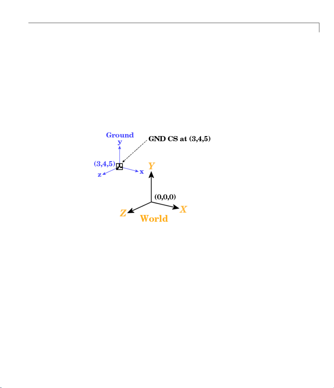
By default the origin of the grounded coordinate sys tem coincides with the origin of the World coordinate system. The Location field of a Ground block’s dialog allows you to move the origin of GND to some other point in the World coordinate system, as in the exampl e “Modeling and Simulating a Simple Machine”.

The GND coordinate system allows you to specify the positions and motions of parts of your machine relative to fixed points in the machine’s surroundings. With a shifted origin, GND remains at rest.

Modeling Rigid Bodies

The SimMechanics Body block enables you to model rigid bodies of finite mass and extent. A body is rigid if its internal parts cannot move relative to one another.

About Body Blocks

A B od y block allows you to specify the following attributes of a rigid body.

Mass Properties. These include the body’s mass, which determines its response to translational forces, and its inertia tensor, which determines its response to rotational torques.

1-11

1 Modeling Mechanical Systems

Body Coordinate Systems. By default a Body block defines three local

coordinate systems, one associated with a body’s center o f gravity, labeled CG, and two others, labeled CS1 and CS2, respectively, associated w ith two otherpointsonthebodythatyoucanspecify.YoucancreateadditionalBody coordinate systems or delete them as necessary.

A Body block’s dialog box allows you to specify a Body CS’s origin (see “Setting a Body CS’s Pos itio n” on pag e 1-14) and orientation (see “Setting a Body CS’s Orientation” on page 1-16). The origin and orientation of a body’s CG CS specify the body’s starting location and orientation. The origins o f the other Body coordinate systems specify the initial locations of other points on the body.

The Body b lock allows flexibility in specifying the origi ns and orientations of Body coordinate systems. You can specify the origin and orientation of a body CS relative to

• The World CS

• Any other CS on the same body

1-12

• The Adjoining CS, the CS on the neighboring body or ground directly

connected by a Joint, Constraint, orDrivertotheselectedBodyCSyou are configuring

This simplifies creation and maintenance of models. The only limitation is that you must specify the origin and location of at least one of a machine’s Body coordinate systems relative to the World CS.

Home Configuration. Once you enter all the needed positions and orientations into the Bodies of your model, your machine is in its home configuration. The body velocities are zero, and any disassembled joints remain disassembled.

Connector Ports. AnyBodyCScandisplayaBodyCSPort. ABodyCSPort allows you to attach Joints, Actuators, and Sensors to a Body. By default, a Body’s CS1 and CS2 coordinate systems each display a Body CS port. You can display a port for any other Body coordinate system as well, including aBody’sCGCS.

Modeling Grounds and Bodies

Creating a Body Block

To create a Body block,

1 Drag a Body block icon from the SimMechanics Bodies Library and drop

it into your model window.

2 Open the Body block’s dialog box.

3 Enter the mass of the body you are modeling in the Mass field.

4 Select the units of mass from the adjacent units list.

5 Enter a 3-by-3 matrix representing the body’s inertia tensor relative to its

center of gravity coordinate system (CG CS) origin and axes in the Inertia field (see “Determining Inertia Tensors for Common Shapes” on page 1-13).

6 Enter the initial positions of the body’s C G and coordinate systems in the

Position tab.

7 Enter the initial orientation of the body’s CG and coordinate systems in

the Orientation tab.

8 Click OK or A pply.

Determining Inertia Tensors for Common Shapes

The following table enables you to determine the inertia tensors for some common shapes. For each shape of mass moments of inertia, I

, I2,andI3,alongthex-, y-,andz-axes of th e shape’s

CG coordinate system.

Shape I

Thin rod of length L aligned

along z

Sphere of radius R

Cylinder of radius R and height h aligned along z

2mR

(m/4)(R2+

/3)

m, the table lists the shape’s principal

/12 mL2/12

/5 2mR2/5 2mR2/5

(m/4)(R

/3)

1-13

1 Modeling Mechanical Systems

Shape I

Rectangular parallelopiped of sides a, b,andc aligned

(m/12)(b

)

(m/12)(a

)

(m/12)(a

)

along x, y, z,respectively

Cone of base radius R and height h along z

Ellipsoid of semiaxes a, b,

(m/4)(3R2/5

)

(m/4)(3R +h

)

(m/5)(b2+c2)(m/5)(a2+c2)(m/5)(a2+b2)

3mR

/10

and c aligned along x, y , z, respectively

The c orresponding inertia tensor for the shape is the following 3-by-3 matrix:

⎛

⎜

⎜ ⎜

⎝

⎞ ⎟

⎟ ⎟

⎠

Working with Body Coordinate Systems

Every SimMechanics body has Body coordinate systems (CSs) attached to it. The location of a body CS is the origin of that CS. The CS’s rectangular x-y-z coordinate axes are rotated at some o rie ntatio n. Y ou set up body CS origins and orientations before running your model. But once the bodies start to move, the origins and orientations of a body’s CSs remain fixe d in the body . The elements of a body’s inertia tensor also remain fixed in the body. Consult “Representing Motion” for more about orienting bodies and body CSs.

1-14

The sections “Managing Body Coordinate Systems” on page 1-17 and “Creating B ody CS Ports” on page 1-18 explain how to create custom Body coordinate sy stems and Body CS ports or delete existing ports.

Setting a Body CS’s Position

The Position tab of a Body block’s dialog box allows you to specify the position of any of a body’s local coordinate systems.

The Tran slate d from Origin of and Components in Axes of lists in the tab together specify which other of your machine’s coordinate systems you

Modeling Grounds and Bodies

use as reference points and orientations to set up the coordinate s ystem s of the body y ou are configuring.

To specify the position of a Body CS,

1 Open the Body block’s dialog box.

The dialog box’s Position tab lists the body’s local coordinate systems in atable.

Each row specifies the position of the coordinate system specified in the Name column.

2 Select the units in which you want to specify the origin of the Body CS from

the CS’s Units list.

3 Specify the reference coordinate systems for the Body CS, i.e., the

coordinate systems relative to which you want to m easure the Body CS origin and the orientation of the Body CS’s coordinate axes. The choices are World, the adjoining CS, and other Body CSs on the same Body.

You must directly or indirectly define all Body CSs by reference to a Ground or to World. Indirect reference means that you specify a Body CS relative to another CS and so on, in a chain of references that ultimately ends in a Ground or World.

1-15

1 Modeling Mechanical Systems

You do this by selecting the origin and orientation of the specification CS from the Body CS’s Translated from Origin o f and Components in Axes of lists, respectively. For example, suppose that you want to specify the position of CS2 relative to another coordinate system , whose origin is at the origin of CS1 but whose axes run parallel to those of the CG CS. Then you would select CS1 from the Translated from Origin of list of CS2 an d CG from the Components in Axes of list of CS2.

1-16

4 Enter a ve

Position

The components of the vector must be in the units that you selected a nd relative to the coordinate system that you selected. For example, suppose that you had selected and World as the CSs specifying the origin and orientation for CS2. Now suppose that you want to specify the loca tion of CS2 as one meter to the right of CS1 along the W orld x-axis. Then you would enter CS2’s position vector.

5 Click Apply to accept the p osition setting or OK to accept the setting and

dismiss the dialog box.

ing a Body CS’s Orientation

Sett

The Orien tation tab of a Body block’s dialog box allows you to specify the orientation of any of a body’s local coordinate systems.

To specify the orientation of a Body CS,

ctor specifying the location of the Body CS in the Origin

Vector [x y z] field of the CS.

m as the unit for specifying CS2’s origin and CS1

[1 0 0] as

Modeling Grounds and Bodies

1 Open the Body block’s dialog box.

2 Select the dialog box’s Orientation tab.

3 Select the units (degrees or radians) in which you want to specify the

orientation of the CS from the CS’s Units list.

4 Selectthecoordinatesystemrelativetowhichyouwanttospecifythe

orientation of the Body CS from the Body CS’s Relative CS list. The choices are World, the adjoining CS, and other Body CSs on the same Body.

5 Select the convention y ou want to use to specify the orientation of the Body

CS from the CS’s Specified Using Convention list.

6 Enter a vector that specifies the orientation of the Body CS relative to

the CS you choose for that purpose, according to the selected specification convention.

7 Click Ap ply to accept the orientation setting or OK to accept the setting

and dismiss the dialog box.

Managing Body Coordinate Systems

You will often need to modify the default Body coordinate systems of a Body block. You might want to connect a Body to more than two Joints, in which case you need not only more Body CSs, but their Body CS ports as well. Connecting Actuators and Sensors to Bodies requires a Body CS and Body CS port for each connection.

The Body coordinate systems tab of a Body block’s dialog box contains a row of buttons that allow you to add, delete, and reorder a Body’s local coordinate systems.

1-17

1 Modeling Mechanical Systems

To use these b

• Delete to re

• Up to move th

• Down to move

Select Add

uttons, select a Body CS in the CS table and select

move the selected CS from the table

e CS’s entry one row up in the CS table

theCS’sentryonerowdownintheCStable

to add a new CS.

Creating Body CS Ports

To add or d and sele table. C

elete a port from a Body block’s icon, open the block’s dialog box ct or clear the CS’s Show Port check box in the dialog box’s Body CS lick OK or Apply to confirm the change.

1-18

Modeling Degrees of Freedom

In this section...

“About Joints” on page 1-19

“Modeling Joints” on page 1-20

“Creating a Joint” on page 1-27

“Modeling Massless Connectors” on page 1-30

“Modeling Disassembled Joints” on page 1-34

About Joints

A SimMechanics joint represents the degrees of freedom (DoF) that one body (the follower) has relative to another body (the base). The base body can be a movable rigid body or a ground. Unl ike a physical joint, a SimMechanics joint has no mass, although some joints have spatial extension (see “Modeling Massless Connectors” on page 1-30).

Modeling Degrees of Freedom

A SimMechanics joint does not necessarily imply a physical connection between two bodies. For example, a SimMechanics Six-DoF joint allows the follower, e.g., an airplane, unconstrained movement relative to the base, e.g., ground, and does not require that the followerevercomeintocontactwith the base.

SimMechanics joints only add degrees of freedom to a machine, because the Body blocks carry no degrees of freedom. Contrast this with physical joints, which both add DoFs (with axes of motion) and remove DoFs (by connecting bodies). See “Counting Model Degrees of Freedom” on page 1-89 for more on this point.

The SimMechanics Joints Library provides an extensive selection of blocks for modeling various types of jo ints. This section explains how to use these blocks.

1-19

1 Modeling Mechanical Systems

Note A SimMechanics joint represents the relative degrees of freedom of

one body relative to another body. Only if a joint is connected on one side to a ground and on the other to a body does the joint represent an absolute DoF of the body with respect to World.

Modeling Joints

Modeling with Joint blocks requires an understanding of the following key concepts:

• Joint primitives

• Joint types

• Joint axes

• Joint directionality

• Assembly restrictions

1-20

Joint Primitives

Each Joint block bundles together one or more joint primitives that together specify the degrees of freedom that a follower body has relative to the base body. The following table summarizes the joint primitives found singly or multiply in Joint blocks.

Primitive Type Symbol Degrees of Freedom

Prismatic

Revolute

Spherical

Weld

One degree of translational freedom along a prismatic axis

One degree of rotational f reedom about a revolute axis

Three degrees of rotational freedom about a pivot point

Zero degrees of freedom

Modeling Degrees of Freedom

Joint Types

The blocks in the SimMechanics Joint Library fall into the following categories:

• Primitive joints

Each of these blocks contains a single joint primitive. For example, the Revolute block contains a revolute joint primitive.

• Composit

These bl specify relativ Gimbal

multiple rotational and translational degrees of freedom of one body

e to another. Some model idealized real joints, for example, the

ejoints

ocks contain combinatio ns of joint primitives, enabling you to

and Bearing joints.

1-21

1 Modeling Mechanical Systems

Others spec the Six-Do the base.

The Custom of rotati prefabri of their p

• Massles

These bl primit

assembled joints

• Dis

ify a bstract combinations of degrees of freedom. For example,

F block specifies unlimited motion of the follower relative to

Joint allows you to create joints with any desired combination onal and translational degrees of freedom, in any order. The cated composite Joints of the Joints library have the type and order

rimitives fixed. See “Axis Order” on page 1-24.

s connectors

ocks represent extended joints with spatially separated joint

ive axes, for example, a Revo lute-Rev olute Massless Connector.

1-22

Modeling Degrees of Freedom

These blocks represent joints not assembled until simulation starts — for example, a Disassembled Prismatic.

See “Assembly Restrictions” on page 1-26 and “Modeling Disassembled Joints” on page 1-34.

Joint Axes

Joint blocks define one or more axes of translation or rotation along which or around which a fo ll ower block can move in relation to the base b lock. T he axes of a Joint block are the axes defined by its component primitives:

• A prismatic primitive defines an axis of translation.

• A revolute primitive defines an axis of revolution.

• A spherical primitive defines a pivot point for axis-angle rotation.

For example, a Planar Joint block combines two prismatic axes and hence defines two axes of translation.

Axis Direction. By default the axes of prismatic and revolute primitives point in the same direction as the z-axis of the World coordinate system (CS). A Joint block’s dialog box allows you to point its prismatic and revolute axes in any other direction (see “Directing Joint Axes” on page 1-28).

1-23

1 Modeling Mechanical Systems

Axis Order. Composite SimMechanics Joints execute their motion one joint

primitive at a time. A joint that defines more than one axis of motion also defines the order in which the follower body moves along each axis or about a pivot. The order in which the axes and/or pivot appear in the Joint block’s dialog box is the order in which the follower body moves.

Different primitive execution orders are physically equivalent, unless the joint includes one spherical or three revolute primitives. Pure translations and pure two-dimensional rotations are independent of primitive ordering.

Axis Span. The span of the primitive axes is the complete space spanned by their combination. For example, one primitive axis defines a line, a nd two primitive axes define a plane.

Joint Directionality

Directionality is a property of a joint that determines the dependence of the joint on the sign of forces or torques applied to it. A joint’s directionality also determines the sign of signals output by sensors attached to the joint. Every SimMechanics joint in your model has a directionality. You must be able to determine the directionality of a joint in order to actuate it correctly and to interpret the output of sensors attached to it.

1-24

A joint’s follower moves relative to the joint’s bas e. The joint’s directionality takes into account the joint type and the direction of the joint’s axis, as follows.

Modeling Degrees of Freedom

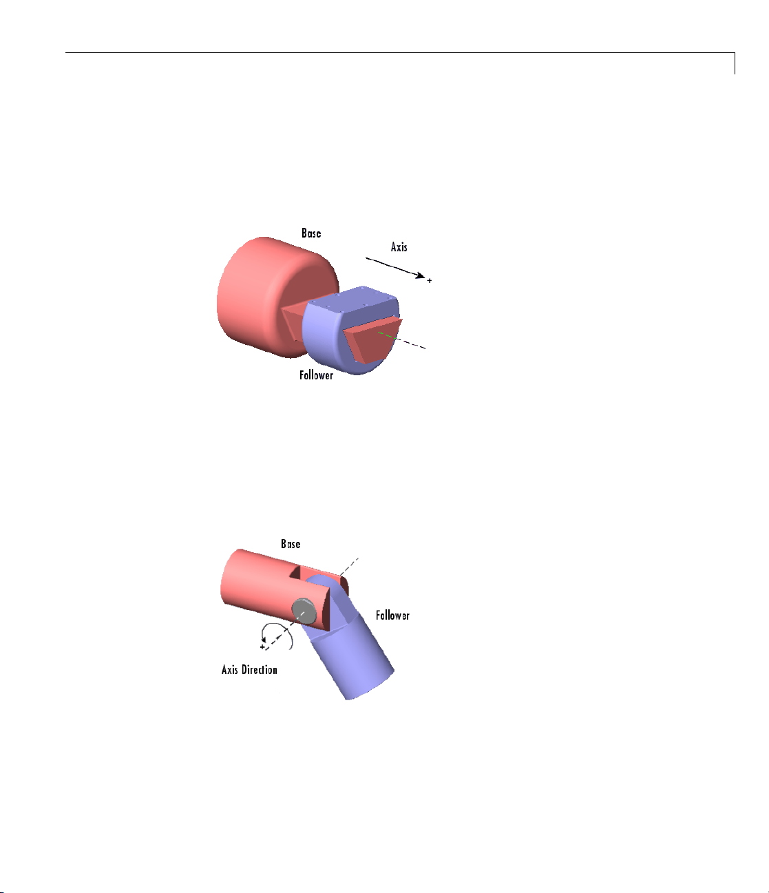
Directionality of a Prismatic Joint. If the joint is prismatic, a positive force applied to the joint moves the follower in the positive direction along the axis of translation. A sensor attached to the joint outputs a positive signal if the follower moves in a positive direction along the joint’s axis of translation relative to the base.

Directionality of a Revolute J oint. If the joint is revolute, a positive torque applied to the joint rotates thefollowerbyapositiveanglearound the joint’s axis of rotation, as determined by the right-hand rule. A sensor attached to the revolute joint outputs a positive signal if the follower rotates by a positive angle around the joint’s axis of revolution, as determined by the right-hand rule.

1-25

1 Modeling Mechanical Systems

Directionality of a Spherical Joint. Spherical joint directionality means

the positive sense of rotation of the three rotational DoFs. P ick a rotation axis, rotating using the right-hand rule from the base Body CS axes. Then rotate the follower Body about that axis in the right-handed sense.

Directionality and Or d er ing of Composite Joint Primitives. Each joint primitive separately has its own directionality, based on the primitive’s type and the direction of its axis of tran slation or rotation. In each case, the follower body of the composite joint moves along or around the joint primitive’s axis relativetothebasebody.

The order of primitives in the composite Joint’s dialog determines the spatial construction of the joint.

The first listed primitive is attached to the base, the second to the first, and so on, down to the follower, which is attached to the last primitive.

• Moving the first listed primitive moves the subsequent primitives in the

list, including the follower, relative to the base.

1-26

• Moving any primitive moves the primitives below it in the list (but not

those above it), as well as the follower.

• Moving the last listed primitive moves only the follower.

Changing the Directionality of a Joint. You can change the directionality

of a joint by either

• Reversing and reconnecting the Joint block to reverse the roles of the base

and follower bodies.

• Reversing the sign (direction) of the joint axis.

Assembly Restrictions

Many joints impose one or more restrictions, called assembly restrictions, on the placement of the bodies that they join. The conjoined bodies must satisfy these restrictions at the beginning of simulation and thereafter within assembly tolerances tha t you can specify (see “Co ntrolling Mach i n e Assembly” on page 2-12). For example, the Body CSs attached to revolute and spherical joints must coincide within assembly tolerances; the Body CSs attached to a Prismatic joint must lie on the prismatic axis within assembly tolerances; the

Modeling Degrees of Freedom

Body CSs attached to a Planar joint must be coplanar with Planar primitives, etc. Composite joints, e.g., the Six-DoF joint, impose assembly restrictions equal to the most restrictive of its joint primitives. See the block reference for each Joint for information on the assembly restrictions, if any, that it imposes.

Positioning bodies so that they satisfy a joint’s assembly restrictions is called assembling the joint.

AllSimMechanicsJointsexceptblocksintheDisassembledJointssublibrary require m anual assembly. Manual assembly entails your setting the initial positions of conjoined bodies to valid locations (see “Assembling Joints” on page 1-29). The simulation assembles disassembled joints during the model initialization phase. It assumes that you have already assembled all other joints before the start of simulation. Hence joints that require manual assembly are called assembled joints. During model initialization and at each time step, the simulation also checks to ensure that your model’s bodies satisfy all assembly restrictions. If any of your model bodies fails to satisfy assembly restrictions, the simulation stops and displays an error message.

Creating a Joint

A joint must connect exactly two bodies. Tocreateajointbetweentwobodies:

1 Select the Joint from the SimMechanics Joints library that best represents

the degrees of freedom of the follower body relative to the base body.

2 Connect the base connector port of the Joint block (labeled B) to the

Body CS origin on the base block that serves as the point of reference for specifying the degrees of fre edom of the follower block.

3 Connect the follo we r connector port of the Joint block (labeled F) to the

Body CS origin on the follower block that serves as the point of reference for specifying the degrees of freedom of the base block.

4 Specify the directions of the joint’s axes (see “Directing Joint Axes” on

page 1-28).

5 If you plan to attach Sensors or Actuators to the Joint, create an additional

port for each Sensor and Actuator (see “Creating Actuator and Sensor Ports on a Joint” on page 1-28).

1-27

1 Modeling Mechanical Systems

6 If the joint is an assembled joint, assemble the bodies joined by the joint

(see “Assembling Joints” on page 1-29).

Directing Joint Axes

By default the prism atic and revolute axes of a joint point in the same direction as the z-axis of the World coordinate system. To change the direction of the axis of a joint primitive:

1 Open the joint’s dialog box and select a reference coordinate system for

specifying the axis direction from thecoordinatesystemlistassociated with the axis p rimitive.

TheoptionsaretheWorldcoordinate system or the local coordinate systems of the base or follower attachment point. Choose the coordinate system that is most convenient.

1-28

2 Enter in the primitive’s axis direction field a vector that points in the

desired direction of the axis in the selected coordinate system.

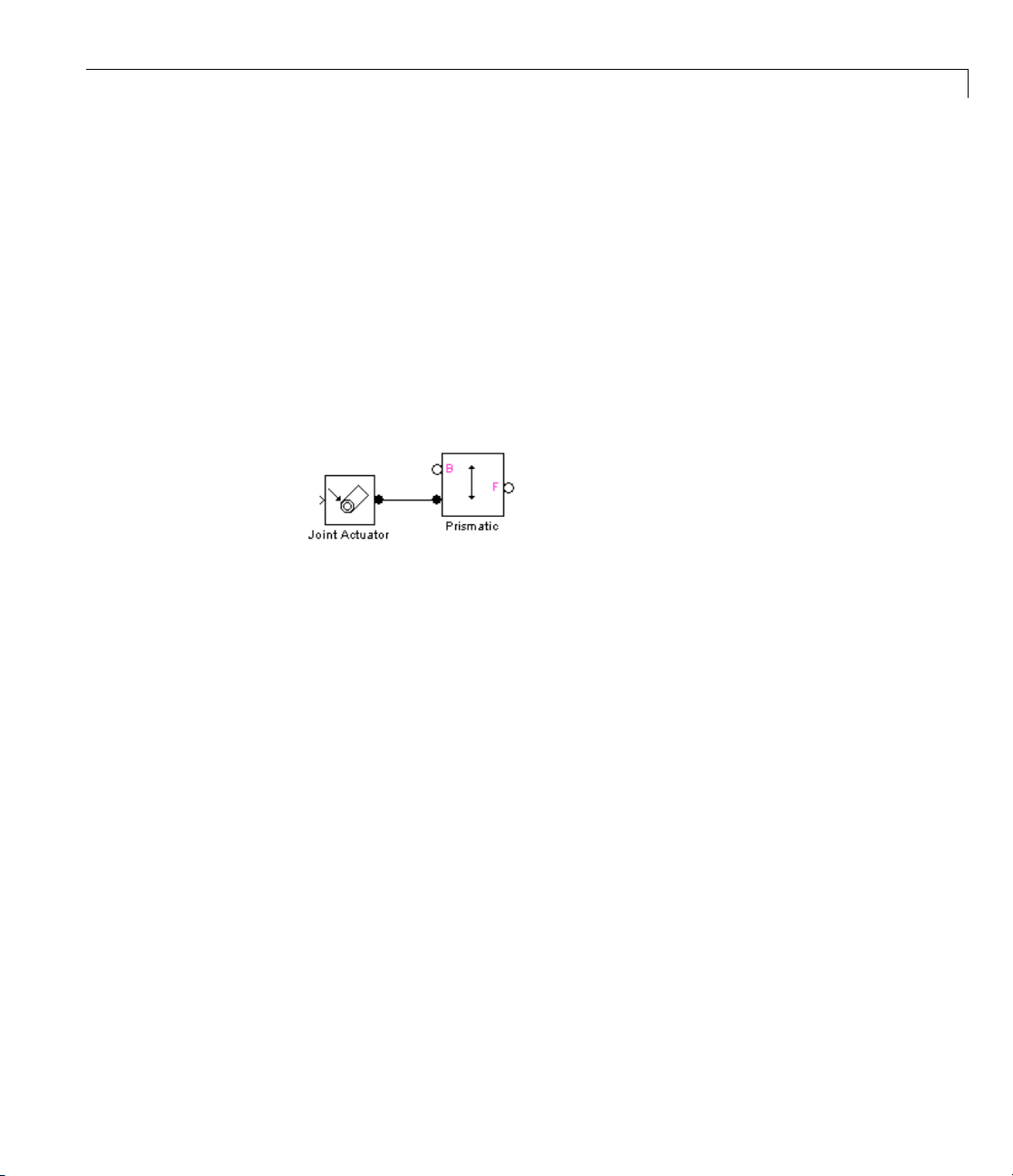
ting Actuator and Sensor Ports on a Joint

Crea

To create additional connector ports on a Joint for Actuators and Sensors, open the Joint’s dialog box and set the Number of sensor/actuator ports to the number of Actuators and Sensors you plan to attach to the Joint.

Modeling Degrees of Freedom

Apply the setting by clicking OK or Apply.

Assembling Joints

You must manually assemble all assembled joints in your model. Assembling a joint requires setting the initial positions of its attached base and follower Body CSs such that they satisfy the assembly restrictions imposed by the joint (see “Assembly Restrictions” on page 1-26). Consider, for example, the “Modeling and Simulating a Clo sed-Loop Machine”.

This model comprises three bars connected by revolute joints to each other and to two ground points. The model collocates the CS o rigins of the Body CS ports connected to each Joint, thereby satisfying the assembly restrictions imposed by the revolute joints.

Assembled Revolute Joint in the Four Bar Mechanism

1-29

1 Modeling Mechanical Systems

Modeling Massle

Massless connec light body to con use a Body block motion might be and the simula avoids global model the conn

A massless co Think of a mas at each end.

tors simplify the modeling of machines that use a relatively

nect two relatively massive bodies. For example, you could

to model such a connector. But the resulting equations of

ill-conditioned, because that connectingbody’smassissmall,

tion can be slow or prone to failure. A massless connector also

inconsistencies that can arise if you use a Constraint block to

ector.

nnector consists of a pair of joints located a fixed distance apart.

sless connector as a massless rod with a joint primitive affixed

ss Connectors

1-30

nitial orientation and length of the massless connector are defined by

The i

tor drawn from the base attachment point to the follower attachment

avec

nt. During simulation, the orientation of the massless connecto r can

poi

nge b ut not its length. In other words, the massless connector preserves

cha

initial separation of the base and follower bodies during machine motion.

the

Modeling Degrees of Freedom

Note You cannot actuate or sense a massless connector.

The SimMechanics Joints/Massless Connectors sublibrary contains these Massless Connectors:

• Two revolute primitives (Revolute-Revolute)

• A revolute primitive and a spherical primitive (Revolute-Spherical)

• Two spherical primitives (Spherical-Spherical)

Creating a Massless Connector

To create a massless connector between two bodies:

1 Drag an instance of a Massless Connector block from the Massless

Connectors sublibrary into your model and connect it to the base and follower blocks.

You can set the direction of the axes of revolute primitives. If necessary, point the axes of the connector’s revolute joints in the direction required by thedynamicsofthemachineyouaremodeling.

2 Assemble the connector by setting the initial positions of the base and

follower body attachment points to the initial positions required by your machine’s structure.

During simulation, the massless connector maintains the initi al separation between the bodies though not necessari ly the initial relative orientation.

1-31

1 Modeling Mechanical Systems

Massless Connector Example: Triple Pendulum

Consider a triple pendulum comprising massive upper and lower bodies and a middle body of negligible mass. The following model uses a Revolute-Revolute massless connector to model such a pendulum.

In this model, the joint axes of the Revolute-Revolute connector have their default orientation along the World z-axis. As a result, the lower arm (Body1) rotates parallel to the World’s x-y plane.

1-32

Modeling Degrees of Freedom

Massless Connector Example: Four Bar Mechanism

The following model replaces one of the bars (Bar2) in the mech_four_bar model from the Demos library with a Revolute-Revolute massless connector.

This model changes the Body CS origins of Bar3 to the following values.

Name Origi

CG [-0.

CS1 [0.

CS2 [0 0

054 0.096 0]

npositionvector

027 -0.048 0]

lated from origin of

Trans

CS1

CS2

ADJ

OINING

(Ground_2)

This creates a separation between Bar3 and Bar1 equal to the length of Bar2 in the original model.

1-33

1 Modeling Mechanical Systems

Try simulating both the original and the modified model. Notice that the massless connector vers ion moves differently, because you eliminated the mass of B ar2 from the model. Notice also that the massless bar does not appear in the animation of the massless connector version of the model.

1-34

Modeling Disassembled Joints

The SimMechanics Joints/Disassembled Joints sublibrary contains a set of joints automatically assembled at the start of simulation; that is, the simulation positions the joints such that they satisfy the assembly restrictions imposed by the type of joint, e.g., prismatic or revolute. Using these joints eliminates the need for you to assem ble the joints yourself.

Disassembled joints differ from assembled joints in significant ways. An assembled joint primitive has only one axis of translation or rev olu ti on or on e spherical pivot point. A disassembled prismatic or revolute primitive has two axes of translation or rotation, one for the base and one for the follower body. A disassembled spherical primitive similarly has two pivot points.

Modeling Degrees of Freedom

Caution Disassembled joints can appear only in closed loops. Each closed loop can contain at most one disassembled joint.

The dialog box for a disassembled joint allows you to specify the direction of each axis.

During model assembly, the simulation determines a common axis of revolution or translation that satisfies model assembly restrictions, and aligns the base and follower axes along the common axis.

Controlling Automatic Assembly and the Assembled Configuration

If your machine contains Joint Initial Condition Actuator (JICA) blocks, the machine is moved from its hom e to its initial configuration by applying the initial condition information to the machine’s joints first. Then any disassembled joints are assembled, leading to the assembled configuration.

During model assembly, the simulation might move bodies connected by assembled joints from their in itia l positions in order to assemble the disassembled joints. The SimMechanics solution to the assembly problem cannot be predicted beforehand, except in simple cases. If you do not want bodies to move during model assembly, use JICA blocks to specify the initial positions of bodies whose positions you want to remain fixed during the assembly process. The resulting assembly will satisfy the initial conditions specified by the JICA blocks.

1-35

1 Modeling Mechanical Systems

Disassembled Joint Example: Four Bar Mechanism

This example creates and runs a model of a disassembled four bar machine.

1-36

Refer to the tutorial, “Modeling and Simulating a Closed-Loop Machine”, and the

1 Disconnect the Joint Sensor1 block from the Revolute3 block.

2 Replace Revolute3 with a Disassembled Revolute block from the

mech_four_bar demo:

Joints/Disassembled Joints sublibrary.

3 Open the Disassembled Revolute dialog box and, under Axis of Action for

both

Base and Follower axes, enter [001]. Close the dialog.

4 Open the Bar2 dialog box and dislocate the joint by displacing Bar2’s CS2

origin from Bar 3 ’s CS1 origin.

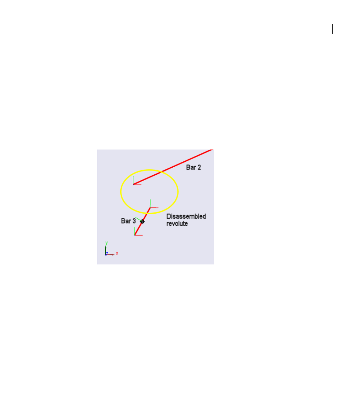
Modeling Degrees of Freedom

Do this by entering a nonzero vector under Origin Position Vector [x yz]for CS2, then changing the Translated from Origin of pull-down

entry to

ADJOINING. CS1 on Bar3 is the Adjoining CS of CS2 of Bar2.

Close the dialog.

5 To avoid circular CS referencing, you must check the Bar3 dialog entry for

CS1 on Bar3. Be sure that CS1 on Bar3 does not reference CS2 on Bar2. Reference it instead to CS2 on Bar3, which adjoins Ground_2.

6 Rerun the model.

Note that the motion is different from the manually assembled case.

1-37

1 Modeling Mechanical Systems

Constraining and Driving Degrees of Freedom

In this section...

“About Constraints” on page 1-38

“Types of Mechanical Constraints” on page 1-38

“What Constraints and Drivers D o” on page 1-39

“Directionality of Constraints and Drivers” on page 1-40

“Solving Constraints” on page 1-40

“Restrictions on Using Constraint and Driver Blocks” on page 1-41

“Constraint Example: Gear Constraint” on page 1-41

“Driver Example: Angle Driver” on page 1-43

About Constraints

The SimMechanics Constraints & Drivers Library provides a set of blocks to model constraints on the relative motions of two bodies. You model the constraint by connecting the appropriate Constraint or Driver block between thetwobodies. Aswithjoints,theblockseachhaveabaseandfollower connector port, with the body connected to the follower port viewed as moving relative to the body connected to the base port. For example, the following model constrains Body2 to move along a track that is parallel to the track of Body1.

1-38

TypesofMechanicalConstraints

Constraint and Driver blocks enable you to model time-independent constraints or time-dependent drivers.

Constraining and Driving Degrees of Freedom

• Constraint and unactuated Driver blocks model scleronomic

(time-independent) constraints.

• Actuated Driver blocks (see “Actuating a Driver” on page 1-62) model

rheonomic (time-dependent) constraints.

Scleronomic constraints lack explicit time dependence; that is, the ir time dependence appears only implicitly through the coordinates x.Rheonomic constraints have explicit time de pendence as well, in addition to impli c it time dependence through the x.

Holonomic constraint functions depend only on body p ositions, not velocities:

(,;)xx = 0

Constraints of the form

can sometimes be integrated into a form dependent only on positions; but if not, they are nonholonomic. For example,

• The one-dimensional rolling of a wheel of radius R along a line (the x-a xis)

imposes a holonomic constraint, x = Rθ.

• The two-dimensional rolling of a sphere of radius R on a plane (the

xy-plane) imposes a nonholonomic constraint, ds = R·dθ,withds

+dy2. This constraint is nonholo nomic because there is not enough information to solve the constraint independently of the dynamics.



(,,,;)xxxx

BBFF

= 0

=dx

What Constraints and Drivers Do

Constrained and driven bodies are still free to respond to externally imposed forces/torques, but only in a way consistent with the constraints.

Constraints and drivers can only remove degrees of freedom from a machine. Constraints and unactuated Drivers prevent the machine from moving in certain ways. Unactuated Drivers hold the constrained degrees of freedom between the connected pair of bodies in their initial state. Actuated Drivers externally impose a relative motion between pairs of bodies, starting with the bodies’ initial state. See “Counting Model Degrees of Freedom” on page 1-89.

1-39

1 Modeling Mechanical Systems

This section discusses modeling constraints and drivers in a general way.

• “Directionality of Constraints and Drivers” on page 1-40

• “Solving Constraints” on page 1-40

• “Restrictions on Using Constraint and Driver Blocks” on page 1-41

The section ends with two examples, “Constraint Example: Gear Constraint” on page 1-41 and “Driver Example: Angle Driver” on page 1-43.

See the reference pages for information on the specific constraint that a Constraint or D riv er block imposes.

Directionality of Constraints and Drivers

Like joints, constraints and drivers have directionality. The sequence of base to follower body determines the directionality of the constraint or driver. The directionality determines how the sign of Driver Actuator signals affects the motion of the follower relative to the base and the sign of sign als output by constraint and driver sensors.

1-40

Solving Constraints

A SimM echanics simulation uses a constraint solver to find the motion, given the model’s Constraint and Driver blocks. You can specify both the constraint solver type and the constraint tolerances used to find the constraint solution. See “Maintaining Constra in ts” on page 2-12 for more in f o rm ation.

Mitigating Constraint Singularities

Some constraints, whether time-independent (Constraints) or time-dependent (Drivers), can become singular when the constrained bodies take on certain relative configurations; for example, if the two body axes line up when the Bodies are connected by an Angle Driver. The simulation slows down as a constraint becomes singular.

If you find a constrained model running slowly, consider selecting the Use robust singularity handling option in the Constraints tab of your machine’s Machine Environment block dialog. See “Handling Mo tion Singularities” on page 2-18.

Constraining and Driving Degrees of Freedom

Restrictions on

The following re in a model:

• Constraint and

cannot contai

• AConstrainto

Constraint E

The mech_ge a Gear Constr

strictions apply to the use of Constraint and Driver blocks

Driver blocks can appear only in closed loops. A closed loop

n m ore than one Constraint or Driver block.

r Driver must connect exactly two Bodies.

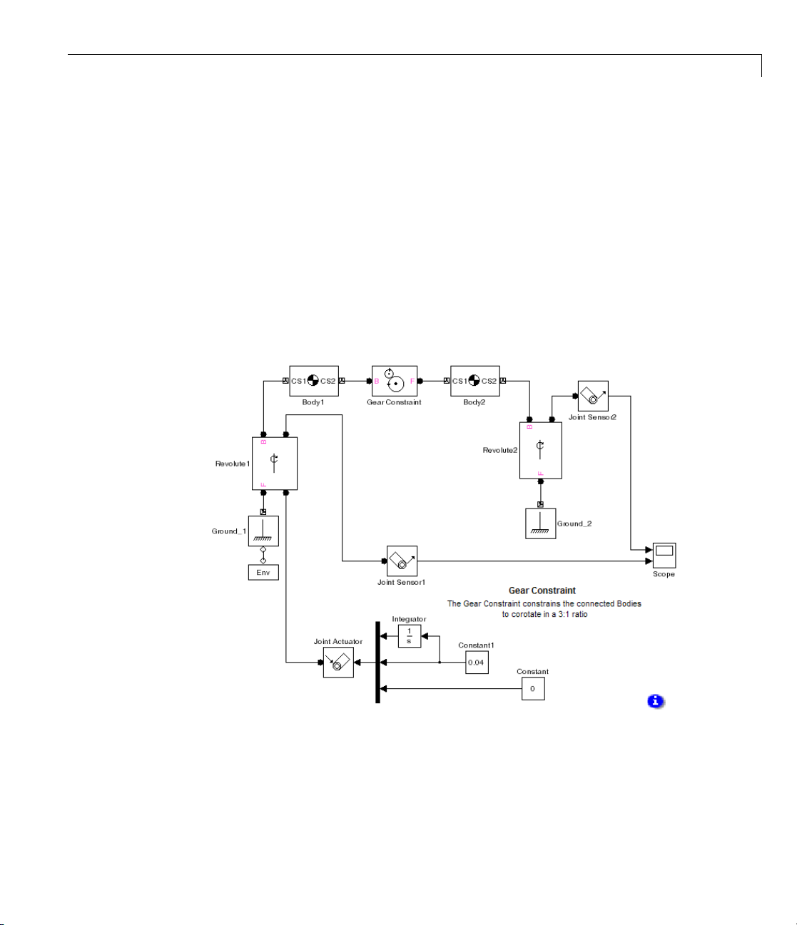
xample: G ear Constraint

model illustrates the Gear Constraint. Open the Body and

aint blocks.

Using Constraint and Driver Blocks

y1 and Body2 have their CG positions 2 meters apart. CS1 and CS2 on

Bod

y1 are collocated with the Body1 CG, and similarly, CS1 and CS2 on

Bod

y2 are collocated with the Body2 CG.

Bod

1-41

1 Modeling Mechanical Systems

The Gear Constraint between them has two pitch circles. One is centered ontheCS2atthebaseBody,whichisBody1,andhasradius1.5meters. The other is centered on CS1 at the follower Body, which is Body2, and has radius 0.5 meters. The distance between CS2 on Body1 and CS1 on Body2 is 2 meters. The sum of the pitch circle radii equals this distance, as it must.

Visualizing the Gear Motion

The model is set up to open the visualization window automatically upon simulation start, with convex hulls, as explained in the SimMechanics Visualization and Import Guide. Start the simulation and watch the CG CS axis triads sp in around. The CG triad at Body2 rotates three times faster than the CG triad at Body1, because the pitch circle centered on Body2 is three times smaller.

You can see the same behavior in the Scope. The upper plot shows the motion of Revolute2, and the lower plot the motion of Revolute1. Note that angular motion is mapped to the interval (-180

, +180o] degrees.

1-42

Constraining and Driving Degrees of Freedom

The Gear Constraint is inside a closed loop formed by

Ground_1–Revolute1–Body1–Gear Constraint–Body–Revolute2–Ground_2

Although Ground_1 and Ground_2 are distinct blocks, they represent different points on the same immobile ground at rest in World. So the blocks form a loop.

Driver Example: Angle Driver

The following two models illustrate the Angle Driver, both without and with a Driver Actuator.

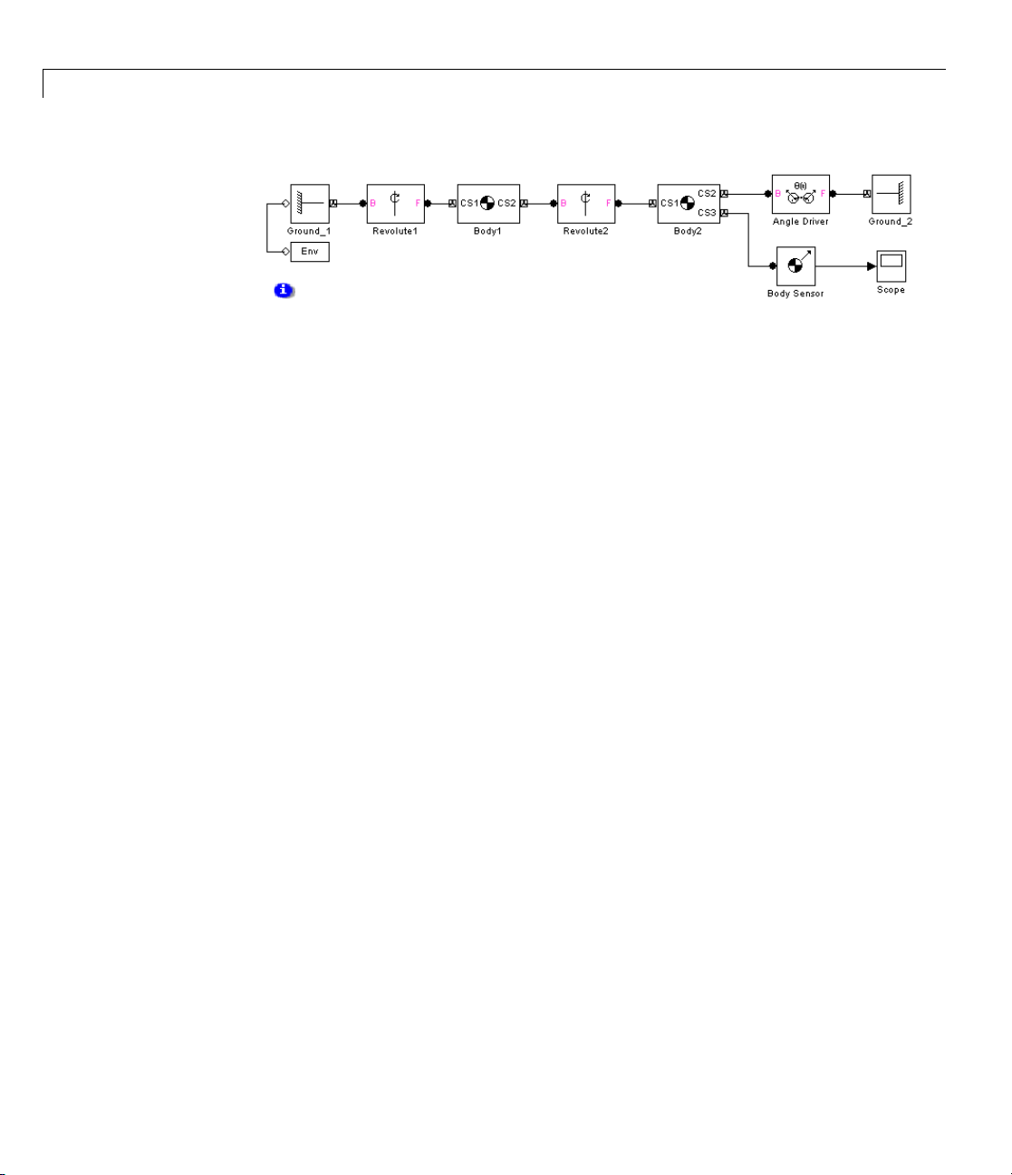
The Angle Driver Without a Driver Actuator

The first is mech_angle_unact.OpentheBody2block.

1-43

1 Modeling Mechanical Systems

The bodies for to Body2 at CS3 velocity vect

The Angle Dri Angle Drive time-indep constant at

m a double pendulum of two rods. The Body Sensor is connected

= CS2 and measures all three components of Body2’s angular

or with respect to the ground.

ver is connected between Body2 and Ground_2. Because the

r is not actuated in this model, it acts during the simulation as a

endent constraint to hold the angle between Body2 and Ground_2

its initial value.

Visualizing the Angle Driver Motion

The model simulati

Visualiz

Start th body mai ground. and thi

is set up to open the visualization window automatically upon

on start, with convex hulls, as explained in the SimMechanics

ation and Import Guide.

e simulation. The upper body swings like a pendulum, but the lower

ntains its horizontal orientation with respect to the horizontal

The Scope measures Body2’s angular velocity with respect to ground,

s remains at zero.

1-44

Constraining and Driving Degrees of Freedom

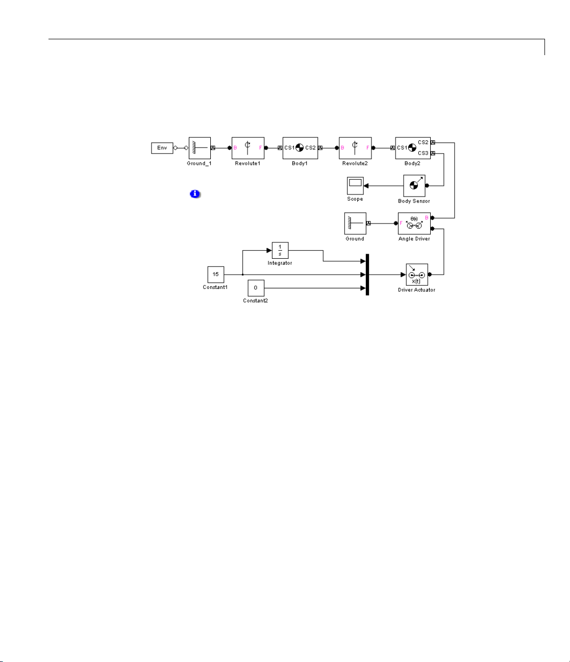
The Angle Driver With a Driver Actuator

The second model is mech_angle_act. Open the Driver Actuator block.

The Driver Actuator drives the Angle Driver block. Here, the Actuator accepts a constant angu la r velocity signal from the Simulink blocks. The Actuator also requires the angle itse lf and the angular acceleration, together with the angular velocity, in a vector signal format. The Angle Driver’s angle signal is added to the angle’s initial value.

The Body Sensor again measures three components of Body2’s angular velocity with respect to the ground. Constant1 drives the angle at 15

/second. While the simulation is running, this angle changes at the constant rate. At the same time, the assembly and the constant length of the two pendulum rods must be maintained by Simulink, while both rods are subject to gravity. As the two axes line up, the mutual constraint between the bodies enforced the D river becomes singular. The simulation slows down.

As in the Gear Constraint model, the two Ground blocks in these models represent points on the same immobile ground at rest in World, so the Angle Driver is part of a closed loop.

1-45

1 Modeling Mechanical Systems

Cutting Machine Diagram Loops

In this section...

“Rules for Valid Machine Diagram Loops” on page 1-46

“Rules for Automatic Loop Cutting” on page 1-46

“Specifying a Loop Joint for Cutting” on page 1-47

“Displaying the Cut Joints” on page 1-47

“For More About Disassembled and Cut Joints” on page 1-47

“For More About Constraints and Drivers” on page 1-47

Rules for Valid Machine Diagram Loops

In a SimMechanics model, you form a closed loop by the closure of SimMechanics blocks, of any type, on themselves. From a starting point, you can trace a path around a closed loop back to the starting point with no jumps or cuts. A closed loop is valid if it contains:

1-46

• AtleastoneJointblock

• No more than one Disassembled Joint block

• No more than one Constraint or Driver block

To simulate a model containing closed loops, the SimMechanics simulation internally co nverts a closed-loop model to an op en-topology tree model. This is accomplished by internally cutting each of the model’s closed loops once, at a joint, constraint, or driver block, then replacing each cut by an additional internal constraint.

Rules for Automatic Loop Cutting

A SimMechanics simulation follows these loop-cutting rules.

• If a loop contains a constraint, driver, or disassembled joint, the simulation

cuts the loop at one of those blocks. Selecting a preferred cut joint has no effect.

Cutting Machine Diagram Loops

• If the loop does not contain a constraint, driver, or disassembled joint, the

simulation cuts the loop at the preferred cut joint if you have specified one.

• If the loop does not contain a constraint, drive r , or disassembled joint, and

you have not specified a preferred cut joint, the simulation cuts the loop at the joint with the most degrees of freedom.

Note A SimMechanics simulation cuts a closed loop at a Disassembled Joint, Constraint, or Driver block, if one or more of these blocks is present, regardless of other Joints also present in the loop or of your preferred cut choice.

Specifying a Loop Joint for Cutting

You can specify a joint to cut if the loop does not contain a disassembled joint, constraint, or driver. Open the joint’s dialog box and select the Mark as the

preferred cut joint check box on the Advanced tab in that joint’s dialog Parameters area.

Displaying the Cut Joints

To display automatically cut joints in your model, select the Mark automatically cut joints check box in the Diagnostics area of the SimMechanics node of your model’s Configuration Parameters dialog. See

“Configuring SimMechanics Simulation Diagnostics” on page 2-18.

For More About Disassembled and Cut Joints

Refer to “Modeling Disassembled Joints” on page 1-34 for more on disassembled joints. Consult “Verifying Model Topology” on page 1-85 to learn more about closed loop analysis.

For More About Constraints and Drivers

A SimMechanics simulation represents a cut Joint, Constraint, or Driver as an additional internal constraint. See “Constraining and Driving Degrees of Freedom” on page 1-38 for more about these specialize d blocks.

1-47

1 Modeling Mechanical Systems

Applying Motions and Forces

In this section...

“About Actuators” on page 1-48

“Actuating a Body” on page 1-50

“Varying a Body’s Mass and Inertia Te ns or” on page 1-53

“Actuating a Joint” on page 1-56

“Actuating a Driver” on page 1-62

“Specifying Initial PositionsandVelocities”onpage1-62

About Actuators

The SimMechanics Actuators & Sensors Library provides a set of Actuator blocks that enable you to apply time-dependent forces and motions to bodies, joints, and drivers. You can also vary a body’s mass and inertia tensor.

1-48

Caution Do not connect an Actuator to a Ground. An error results if you attempttosimulateorupdateamodelcontaining such a connection. This is because ground is immobile and cannot be actuated.

You can use Actuator blocks to perform the following tasks:

• Apply a time-varying force or torque to a body o r joint.

• Specify the position, velocity, and acceleration of a joint or driver as a

function of time.

• Specify the initial position and velocity of a joint primitive.

• Specify the mass and/or inertia tensor of a body as a function of time.

In general, actuators can apply any combination of forces and motions to a machine provided that

• The applied forces and motions are consistent with each other and with the

machine’s g eometry, constraints, and assembly restrictions.

Applying Motions and Forces

• The actuation signals representing these forces and motions remain

consistent when differentiated or integrated. See “Stabilizing Numerical Derivatives in Actuator Signals” on page 1-49.

• Itispossibletofindauniquesolutionforthemotionofeachactuated

degree of freedom (D oF).

Stabilizing Numerical Derivatives in Actuator Signals

To actuate a phys ical system m od eled by blocks, you often need to differentiate an incoming Simulink actuation signal.

Simulink provides a Derivative block for numerical differentiation of a signal. However, this block’s output is sometimes not stable or accurate enough for Physical Modeling purposes. Recommended alternatives to the Derivative block include the following.

Integrating Higher Derivative Signals. Start by specifying the highest derivative signal (such as an acceleration), then integrate this signal to obtain lower derivative signals (such as a velocity) using the Integrator block.

Transforming Signals with Transfer Functions. To differentiate a signal, use a transfer function block (Transfer Fcn). This block actually performs a Laplace transform convolution to smooth the output, which is not exactly the derivative.

You can eliminate this drawback by filtering the original signal f,then defining exact derivatives dF/dt, etc., of the filtered signal F by adding higher orders to the transfer function numerator. The order of the denominator should be equal to or greater than the number of output signals. Use the filtered signal F (instead of f), as well as the filtered derivatives.

In this example, the constant τ represents a smoothing time. The transfer functions define a filtered signal and its first derivative, two signals in all. Therefore, the transfer function deno minator should be seco nd order or high er.

1-49

1 Modeling Mechanical Systems

Examples of Numerical Deriv atives of Actuator Signals

A SimMechanics example requiring numerical derivatives is motion actuation of a joint, which requires position, velocity, and acceleration of each joint primitive as a function of time. You specify this information as a set of Simulink signals, which you can stabilize with one of the previous methods.

The transfer function method is illustrated by the model. For an example of the derivative-integration method, see the

mech_body_driver model.

mech_stewart_control

Actuating a Body

You can use the Body Actuator to apply forces and/or torques, but not motions, to bodies. (You can apply motions to a body indirectly, using Joint Actuators. See “Applying Motions to Bodies” on page 1-52.)

To actuate a body,

1 If there is not already a n unused connector port available for the Actuator

create a Body CS port on the Body for the Actuator. See the Body block reference if you need to learn how.

2 Drag a Body Actuator block from the Sensors & Actuators library into your

model and connect its output port to a Body CS port on the Body.

3 Open

4 Choose to apply a force or torque to the body:

the Actuator’s d ialog box.

• Select the Applied force check box if you want to apply a force to the

body, and select the units of force from the adjacent list.

1-50

Applying Motions and Forces

• Select the Applied torque check box if you want to apply a torque to

the body, and select the units of torque from the adjacent list.

5 Selectthecoordinatesystemusedtospecify the applied torque from the

With respect to CS list.

The list allows you to choose either the World CS or the Body CS of the port to which you attached the Actuator.

6 Create vector signals that specify thevalueoftheappliedtorqueandforce

at each time step.

You can use any Simulink source block (for example, an Input port block or a Sine Wave block) or combination of Simulin k blocks to cre ate the Body Actuator signal. You can also use the output of a Sensor block connected to the Body as input to the Actuator, thereby creating a feedback loop. Such loops are useful for modeling springs and dampers (see “Validating Mechanical Models” on page 1-85).

7 Connect the force and/or torque signal to the input port of the Actuator.

If you are applying both a force and a torque to the body, connect the force and torque signals to the inputs of a two-input Mux block. Then connect the o utput of the Mux block to the input of the Actuator.

Body Actuator Example: Pure Kinetic Friction

The mech_ballistic_kin_fric model in the Demos library provides an example of how to implement pure kinetic friction. This type of friction is a continuous force that depends on a body’s motion relative to a medium (such as air), as well as on physical characteristics of the body. K inetic friction, unlike “stiction,” involves no “sticking” or locking of motion, and the friction is not discontinuous. While you could use the Joint Stiction Actuator, this is not necessary. This model applies air friction or drag to a projectile w ith a Body Actuator.

1-51

1 Modeling Mechanical Systems

Open the Air Drag subsystem. If you double-click the block, a mask dialog box opens asking for the drag coefficient Look under mask, the subsystem itself appears:

Cd. If you right-click the block and select

1-52

The Air Drag subsystem computes the air friction according to a standard air friction m odel. (See the Aerospace Blockset documentation for more information.) The drag always opposes the projectile’s motion and is proportional to the product of the air density, the projectile’s cross-sectional area, and the square of its speed.

Run the model with the default drag coefficient (zero). The XY Graph window opens to plot the parabolic path o f the projectile. Now open the Air Drag dialog again and experiment w ith different drag coefficients C smallvaluessuchasC

= 0.05. For a rigid sphere, Cdis two. The effect of the

. Start with

drag is dramatic in that case.

Applying Motions to Bodies

The Body Actuator block cannot actuate a Body with motion signals. But y ou can construct such body motion actuators with a combination of other blocks. See “Joint Actuator Example: Body Driver” on page 1-58.

Applying Motions and Forces

Varying a Body’ s

The Variable Mas mass and/or iner functions with

Caution The Va thrust forces particular d apply these f

The variabl apply force by initial c affect its forces/to

The Varia mass and r body at a mass and externa invisib mass, n two con

s/torques on the body. When a body’s motion is determined only

onditions, changing the mass or inertia tensor of a body does not

motion, because the variable mass/inertia actuator does not apply

rques to the body.

ble Mass & Inertia Actuator block changes the actuated Body’s

otational inertia by attaching an invisible body to the actuated

particular Body coordinate system (CS). This invisible body has a

an inertia tensor that vary in time as specified by the Actuator’s

l Simulink signal. The simulation treats the actuated body and the

le body as a single composite body. The composite body has a new

ew center of gravity ( CG ), and new inertia tensor com po unded from its stituent bodies.

s & Inertia Actuator block gives you a w a y to vary a body’s

tia tensor as external functions of time. You specify these

incoming Simulink signals.

riable Mass & Inertia Actuator block does not apply any

or torques to the Body so actuated. Mass loss or gain in a

irection results in thrust forcesandtorquesonthebody. Youmust

orces/torques to the Body separately with B ody Actuator blocks.

e mass/inertia actuator affects a body’s motion only when you

Mass and Inertia Tensor

1-53

1 Modeling Mechanical Systems

You can add multiple Variable Mass & Inertia Actuator blocks to one Body. In that case, the simulation treats the actuated body and all attached invisible bodies as a single composite body. This composite body’s mass, CG, and inertia tensor are compounded from its constituent bodies.

1-54

Attaching Variable Mass and Inertia Bodies to a Visible Body

To vary the mass and/or inertia tensor of a Body with this Actuator:

1 From the Sensors & Actuators library, drag a Variable Mass & Inertia

Actuator block into your model.

2 Attach the Actuator’s connector port to the Body CS on the Body where you

want the invisible variable mass to be. If a suitable Body CS port does not exist on the Body, open its dialog and create one.

3 Create an external Simulink signal to model the time-varying mass and/or

inertia tensor for this invisible body. Connect it to the Variable Mass & Inertia Actuator b lock’s Simulink input port.

This Simulink signal can have one, nine, or ten components, depending on whether you are varying the mass only, the inertia tensor only, or both.

Applying Motions and Forces

Example: Simple Rocket

The following model simulates a simple rocket. It treats the rocket as a point mass moving upward (+y direction) with an exhaust pointing downward (-y direction). The rocket losesmassataconstantrate.

The Rocket block is the point mass. The Thrust Velocity block represents the downward exhaust and, multiplied by the mass loss represented by the Fuel Loss block, actuates the Rocket body with a thrust force pointing upward. The Thrust block (a body actuator) applies this force at the local Body CS, which, for a point rocket, is identical to the Rocket’s CG CS.

The same mass loss from the Fuel Loss block that produces the thrust force also must vary the rocket’s mass directly. The Variable Mass Actuator block accomplishes this by feeding the same mass loss signal to the Rocket block.

1-55

1 Modeling Mechanical Systems

Actuating a Joint

You individually actuate each of the prismatic and revolute primitives of an assembled joint with a Joint Actuator. You can apply

• Forces or translational motions (but not both) to prismatic primitives

• Torques or rotational motions (but not both) to revolute primitives

Caution You cannot actuate spherical or weld primitives, disassembled

joints, or massless connectors.

Do not connect multiple Actuators to the same joint primitive. An error results if you attempt to update or simulate a model containing such a connection.

Exception: You can apply a Joint Initial Condition Actuator and force or torque actuation (including stiction) to the same primitive. You cannot apply a Joint Initial Condition Actuator and motion actuation to thesameprimitive. See “Specifying Initial Positions and V elocities” on page 1-62.

1-56

Actuating a Joint Primitive

Tip If you have multiple forces/torques or motions you want to apply to a

joint primitive, sum their values as Simulink signals first, then apply the net result as the input to the Joint Actuator.

To actuate a prismatic or revolute joint primitive of an assembled joint:

1 Create an Actuator port on the Joint block for the primitive (see “Creating

Actuator and Sensor Ports on a Joint” on page 1-28).

2 Drag a Joint Actuator or Joint Stiction Actuator from the Sensors &

Actuators library into your model and connect its output port to the Actuator port on the Joint.

remaining steps in this procedure apply to the creation of a standard

The

nt Actuator. For information on creating a stiction actuator, which

Joi

Applying Motions and Forces

applies classical Coulombic friction to a prismatic or revolute joint, see the Joint Stiction Actuator block reference page.

3 Open the Joint Actuator’s dialog box.

4 Select the primitive you want to actuate from the Connected to primitive

list on the dialog box.

5 SelectthetypeofactuationyouwanttoapplyfromtheActuate with

pull-down menu, either

6 If you are actuating a prismatic primitive:

Generalized Forces or Motion.

• If you selected

Generalized Forces as the actuation type, select the

units of force from the Applied force units list.

• If you selected

Motion as the actuation type, select the units for each

motion to be actuated (position, velocity, acceleration).

7 If you are actuating a revolute primitive:

• If you selected

Generalized Forces as the actuation type, select the

units of torque from the Applied torque units list.

• If you selected

Motion as the actuation type, select the units for each

motion to be actuated (angle, angular velocity, angular acceleration).

8 Click OK to apply your choices and dismiss the dialog box.

Each joint primitive that you motion-actuate is lost as a true degree of freedom in your machine. That is because the DoF can no lo nger respond freely to externally applied forces or torques. See “Co unting Model Degre es of Freedom” on page 1-89.

9 Create a signal that specifies the applied force, torque, or motions at each

time step.

You can use any Simulink source block or any combination of blocks to create the actuator signal. You can also connect the output of a Sensor block attached to the Joint to the Actuator input, thereby creating a feedback loop. You can use such loops to model springs and dampers attached to the joint.

1-57

1 Modeling Mechanical Systems

A force or torque signal must be a scalar signal. A motion signal must be a 1-D array signal comprising three components: position, velocity, and acceleration. The directionality of thejointdeterminestheresponseofthe follower to the sign of the actuator signal (see “Joint Directionality” on page 1-24).

10 Connect the Actuator signal to the Actuator port on the Joint.

Joint Actuator Example: Body Driver

The mech_body_driver model illustrates the use of Joint Actuators to create a custom driver.

1-58

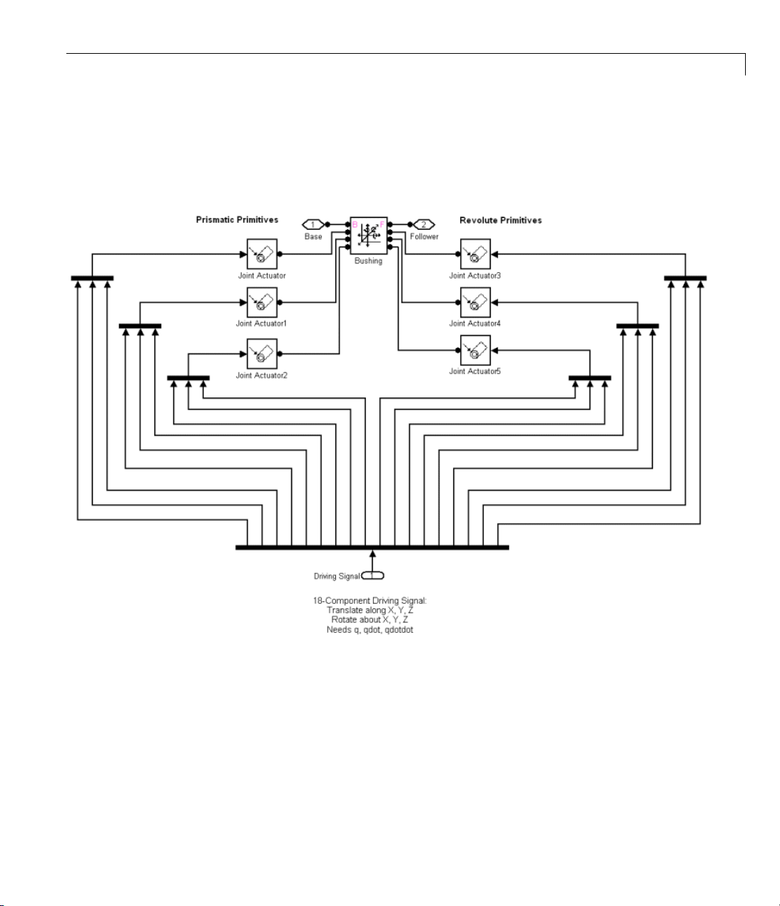
Applying Motions and Forces

The Body Driver subsystem accepts an 18-component signal that feeds the coordinates, velocities, and accelerations for all six relative DoFs between Body and Body1. The subsystem uses a Bushing block that contains three translational and three rotational primitivestorepresenttherelativeDoFs:

You can modify the body driver to move only one of the bodies, thereby creating a motion actuator. To move B od y1 relative to World, for example, remove the blocks Body and Weld and connect the subsystem Body Driver directly to Ground.

1-59

1 Modeling Mechanical Systems

Joint Stiction Actuator Example: Mixed Static and Kinetic Friction

Tip You should use the Joint Stiction Actuator block only if you need static

(locking) friction that removes one or more degrees of freedom from your machine.

You can model pure kinetic friction (damping) with other Actuator and Sensor blocks. See “Actuating a Body” on page 1-50 and “Adding Internal Forces” on page 1-74.

The mech_dpen_sticky model in the Demos library illustrates a driven double pendulum, with “sticky” friction or stiction applied to both revolute joints with the Joint Stiction Actuator block.

1-60

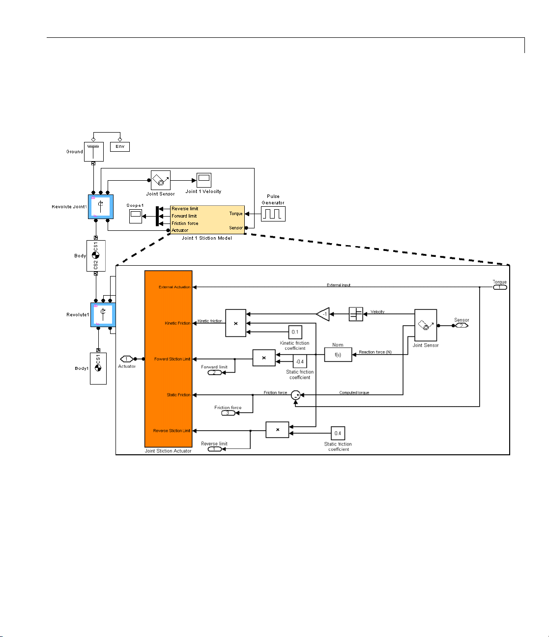
Applying Motions and Forces

Open the unmasked Joint1 or Joint2 Stiction Model blocks (marked in yellow) to view the subsystems:

Each Stiction subsystem contains a Joint Stiction Actuator block (marked in orange) that requires static and kinetic friction coefficients via their respective blocks. For either revolute, an angular velocity threshold, specified through the block dialog, determines if a joint locks. Once locked, the joint cannot move until a combination of forces reaches a threshold specified by the

Forward Stiction Limit or Reverse Stiction Limit.

1-61

1 Modeling Mechanical Systems

Run the m odel with different kinetic and static friction coefficients and different velocity thresholds. View the results in the Scope blocks and through a visualization window. You can find more details on how SimMechanics stiction works by consulting the Joint Stiction Actuator block reference page.

Actuating a Driver

Actuating a Driver with a Driver Actuator allows you to specify the time dependence of the rheonomic constraint applied by the Driver.

To actuate a Driver:

1 Create an additional connector port on the Driver for the Actuator.

Create the additional port in the same way you create an additional Sensor/Actuator port on a Joint (see “Creating Actuator and Sensor Ports on a Joint” on page 1-28).

2 Drag an instance of a Driver Actuator from the Sensors & Actuators library

into your model.

1-62

3 Connect the Actuator’s output port to the Actuator port on the Driver.

4 Create a signal that specifies the time dependence of the Driver constraint.

5 Connect the actuation signal to the input port of the Driver Actuator.

Specifying Initial Positions and Velocities

The Joint Initial Condition Actuator (JICA) block allows you to specify the initial positions and velocities of unactuated joints and hence the bodies attached to them. You can use JICA blocks to

• Specify nonzero initial joint velocities

The default initial velocity of a joint primitive is zero. You m ust use a JICA block to specify a joint’s initial velocity if the initial velocity is not zero.

• Override the initial position settings of a body pair

TheCGCSoriginsettingsinthedialogboxesofBodyblocksspecifythe bodies’ initial positions. Using JICA blocks, you can override these initial

Applying Motions and Forces

body positions by resetting their relative positions in the Joints connecting them.

Your model simulation starts with your machines at first in their home configurations, defined by the Body dialog data. It then transforms your machines to their initial configurations by applying JICA data.

Caution You cannot simultaneously actuate a joint primitive with a Joint Initial Condition Actuator and motion actuation from a Joint Actuator block.

Using JICA Blocks

Specifying initial conditions on a joint p rimitive is a special kind of actuation, one that occurs only once at the beginning of simulation. That is why the JICA block resides in the Sensors & Actuators library.

Note A JICA block, unlike other Actuators, does not have an input port. The JICA’s dialog box specifies the Actuator input completely.

With a JICA block, you can specify the initial positions and velocities of any combination of prismatic and revolute primitives within a given Joint. (You cannot specify ICs for spherical and w eld primitives.)

To specify the initial velocity and/or position of a joint primitive:

1 Drag a JICA block from the Sensors & Actuators library and drop it into

your model window.

2 Create an additional connector port on the Joint block containing the

primitive whose initial condition you want t o specify.

3 Connect the connector port on the JICA block to the new connector port on

the Joint block.

1-63

1 Modeling Mechanical Systems

Caution Do not connect the JICA block to the Joint ports marked "B" or

"F" (base or follower). These ports are intended for connecting to Bodies.

4 Open the JICA block’s dialog box. From the primitive list for the Joint,

choose the primitives you want to actuate by selecting their check boxes.

5 Enter the init ial positions of the actuated primitives, relative to the Body

CSs attached to the Joint, in the Position field.

From the pull-down menu on the right, select Units for the initial positions.

6 Enter the initia l velocities of the actuated primitives, re la t ive t o the Body

CSs attached to the Joint, in the Velocity field.

From the pull-down menu on the right, select Units for t he initial velocities.

7 Click Apply or OK.

1-64

JICA Example: A Simple Pendulum

Open mech_spen from the Demos library, then open the Sensors & Actuators library. Follow the steps from the preceding section, “Using JICA Blocks” on page 1-63, to connect one Joint Initial Condition Actuator block to the Revolute block and configure it. This Joint contains only one primitive, which is the primitive listed in the JICA dialog box.

R1,

Applying Motions and Forces

Set the initial conditions in two ways and compare the resulting simulations in the scope:

1 First set the initial Position (angle) to 60 deg,whichis60

the left horizontal (30 Velocity to

0 deg/s.

clockwise from vertically down), and set the initial

down from

1-65

1 Modeling Mechanical Systems

2 Run the simulation for one second. Note in the scope that the initial angle

(yellow curve) is displaced upward to 60

, while the i nitial velocity (purple

curve) still s tarts at zero.

3 Now reset the initial Velocity to 30 deg/s, leaving the initial Position

(angle) at

4 Rerun the simulation for one second. Note in Scope that the initial angle

is still displaced upward to 60 upward to 30

60 deg.

/sec.

, but the initial velocity is also displaced

1-66

Applying Motions and Forces

The joint directionality is assigned in mech_spen so that the positive rotation axis is the +z-axis. Looking from the front, positive rotation sw ings down and right, counterclockwise.

1-67

1 Modeling Mechanical Systems

Sensing Motions and Forces

In this section...

“About Sensors” on page 1-68

“Sensing Body Motions” on page 1-69

“Sensing Joint Motions and Forces” on page 1-70

“Sensing Constraint Reaction Forces” on page 1-71

About Sensors

The SimMechanics Sensors & Actuators library p rovides a set of Sensor blocks that enable you to measure

• Body motions

• Joint motions and forces or torques on joints

• Constraint reaction forces and torques

1-68

All Sensor output is defined with respect to a fixed, conventional “zero.” See “Home C onfiguratio n and Position-Orientation Measurements” on page 1-68.

Tip You can feed Sensor output back into Actuator blocks to model springs, dampers, and other mechanical devices that depend on force feedback. See “Actuating a Body” on page 1-50, “Actuating a Joint” on page 1-56, “Adding Internal Forces” on page 1-74, and “Validating Mechanical Models” on page 1-85.

Home Configuration and Position-Orientation Measurements

The Body and Joint Sensor blocks can measure the position and/or orientation of bodies and degrees of freedom. They make these measurements relative to the home configuration of the machine, the machine state before the application of initial condition actuators and assembly of disassembled joints. Thus motion sensors include the effect of the latter, which act before the simulation starts.

Sensing Motions and Forces

For furthe r discussion, see “Modeling Disassembled Joints” on page 1-34 and “Specifying Initial Positions and Velocities” on page 1-62, and “Kinematics and the Machine’s State of Motion”.

Sensing Body Motions

To sense the position, velocity, or acceleration of a body represented by a Body block with a Body Sensor:

1 If the Body block does not have a spare local coordinate system with a

Body CS port, create one (see “Managing Body Coordinate Systems” on page 1-17).

2 Drag a Body Sensor block from the Sensors & Actuators library into your

model.

3 Connect its connector port to a spare Body CS port on the Body.

4 Open the Sensor’s dialog box.

1-69

1 Modeling Mechanical Systems

5 Selectthecoordinatesystemrelativetowhichthesensormeasuresits

output from the With respect to CS list.

6 Select the check boxes next to the motions that you want to sense ( see the

Body Sensor block reference page).

7 Ifyouhavechosentosensemorethanonetypeofmotionandwantthe

Sensor to multiplex the motions into a single output signal, select the Output selected parameters as one signal check box.

8 Click OK or A pply.

9 Connect the output of the Body Sensor block to a Simulink Scope or other

signal sink or to a motion feedback loop, depending on your needs.

Sensing Joint Motions and Forces

The Joint Sensor block enables you to measure the motions of degrees of freedom. It can also measure the relative forces and torques between the bodies connected to the joint. These include the computed force or torque (the force or torque needed to reproduce the joint’s motion) and the reaction force and torque on a joint primitive. (You cannot measure the computed force or torque on a spherical or weld primitive.) You must connect a separate Joint Sensor block to a Joint block for each joint primitive that you want to sense.

1-70

To sense the motions, forces, and torques of a joint primitive contained by a Joint block:

1 If the Joint block does not have a spare Sensor port, create one (see

“Creating Actuator and Sensor Ports on a Joint” on page 1-28).

2 Drag a Joint Sensor block from the Sensors & Actuators library into your

model.

3 Connect its connector port to the spare Sensor port on the joint.

4 Use the Sensor’s dialog box to configure the Sensor to measure the motions,

forces, and torques that you want to measure (see the Joint Sensor block reference page).

5 Connect the output of the Joint Sensor block to a Simulink Scope or other

signal sink or to a motion feedback loop, depending on your needs.

Sensing Motions and Forces

Sensing Constraint Reaction Forces

The Constraint & Driver Sensor block enablesyoutomeasurethereaction forces and torques induced on the constraints modeled by SimMechanics Constraint and Driver blocks.

To sense the reaction force and/or torque induced by a constraint or driver,

1 If the Constraint or Driver does not have a spare Sensor port, create one.

2 Drag a Constraint & Driver Sensor block from the Sensors & Actuators

library into your model.

3 Connect its

connector port to a Sensor port on the Constraint or Driver

block.

4 Open the Sensor block’s dialog box.

5 Select the body (follower or base) on which to measure the reaction force

from the Reactions measured on list.

6 Select the coordinate system relativetowhichtheSensormeasuresits

output from the W ith respect to coordinate system list.

7 Select the Reaction torque check box if you want the Sensor to output

the reaction torque on the base (or follower) body.

1-71

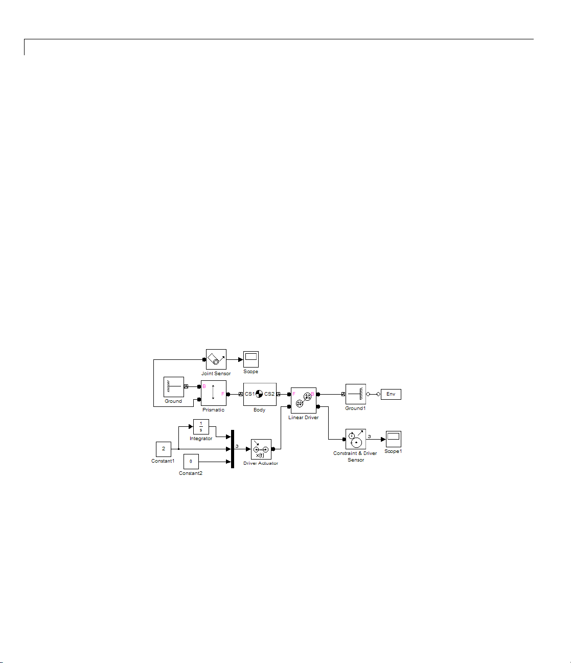
1 Modeling Mechanical Systems

8 Select the Reaction force check box if you want the Sensor to output the

reaction force on the base (or follower) body.

9 Ifyouhavechosentooutputbothreactionforceandtorqueandwantthe

Sensor to multiplex them into a single output signal, select the Output selected parameters as one signal check box.

10 Click OK or Apply. Connect the output of the Constraint & Driver Sensor

block to a Simulink Scope or other signal sink or to a motion feedback loop, depending on your needs.

Not all the reaction force/torque components are significant. Only those components projected into the subspace of constrained or driven degrees of freedom (DoFs) are physical. Components orthogonal to the constrained or driven degrees of freedom are not physical.

Example: Linear Driver

In this example, you drive a body along the x-axis, but only allow it a prismatic DoF tilted at an angle in the x-y plane. Construct the following model.

1-72

Configure the Constraint & Driver Sensor to measure only the reaction force, not the torque. Configure the Linear Driver to drive the Body along the W orld x-axis, but set up the Prismatic with a primitive axis along (1, 2, 0). The body can then move only along this axis, but is driven along the horizontal x-axis. Measure all motions and forces in World. Leave all other settings at default.

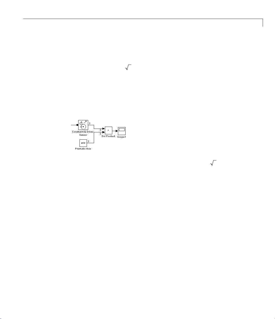
Sensing Motions and Forces

Open the Scopes and run the model. The measured reaction force lies along the x-axis, with a value of -19.62 N (newtons) = -2mg. Because the constrained DoF is not parallel to the x-axis, you need to project the reaction force along

the unit vector (1, 2, 0)/

defining the direction of the prismatic primitive

to obtain the physical part.

Add to the model the Simulink blocks that form a dot product between the reaction force signal (three components) and the prismatic unit vector (also three components). (You can define a workspace vector for this axis and use it in both the joint and the dot product.) Reconnect Scope1 to measure this physical component of the reaction force.

The physical component of the reaction force is -(19.62 N)·(1/5)=-8.77N. The component of the reaction force orthogonal to (1, 2, 0) is not physical.

1-73

1 Modeling Mechanical Systems

Adding Internal Forces

In this section...

“About Force Elements” on page 1-74

“Inserting a Linear Force Between Bodies” on page 1-74

“Inserting a Linear Force or Torque Through a Joint” on page 1-76

“Customizing Force Elements with Sensor-Actuator Feedback” on page 1-78

About Force Elements

Internal forces are forces the machine applies to itself as a result of its own motion. Unlike actuation forces, you do not apply these forces from outside the machine with Simulink signals. The body motions instead generate the forces and torques directly.

The Force Elements library provides ready-made blocks to represent certain kinds of internal forces and torques acting between bodies. You can also create y our own customized sensor-actuator feedback loops to model springs, dampers, and more complex internal force s.

1-74

Inserting a Linear Force Between Bodies

A generalized linear force between two bodie s is a linear function of the two bodies’ relative displacement vector r and relative velocity v,withconstant coefficients. The Body Spring & Damper block models a force acting between two bodies along the axis r connecting them:

F =-k(r - r

The block is connected on either side to Bodies at a Body coordinate system (CS). The displacement r is a vector from one Body CS on one Body to the other Body CS on the other Body. Newton’s third law requires that the forces that the bodies exert on one another be equal and opposite.

The common physical s ystem this force modelrepresentsisaspring-damper combination, where the damper is a dashpot acting only along the spring axis. The damping is solely a function of the component v

)-bv

of the velocity

Adding Internal Forces

vector projected along the displacement r . (Thus the damping in this block cannot represent the damping due to a viscous medium, because there is no damping force perpendicular to the spring axis. See “Inserting a Linear Force or Torque Through a Joint” on page 1-76.)

You enter the constant parameters r dialog. r

is the spring’s natural length, the length it has when no forces

, k,andb in the Body Spring & Damper

areactingonit. Thespringconstantk and damping constant b should be nonnegative.

To complete a linear force model between bodies, you need to model the translational d eg ree s of free do m (DoFs) between them, as the Force Element block itself does not represent these DoFs. You can use any Joint block containing at least one prismatic primitive to represent translational motion. The two Bodies, the Joint, and the Body Spring & Damper must form a closed loop.

The following block diagram represents two Bodies w ith a damped spring between them. The Custom Joint represents the bodies’ relative translational DoFs with three prismatic primitives. In this case, CS2 and CS3 on Body1 are the same, and CS2 and CS3 on Body2 are the same. Thus, the Joint is connected to the same Body CSs that define the ends of the spring-damper axis.

1-75

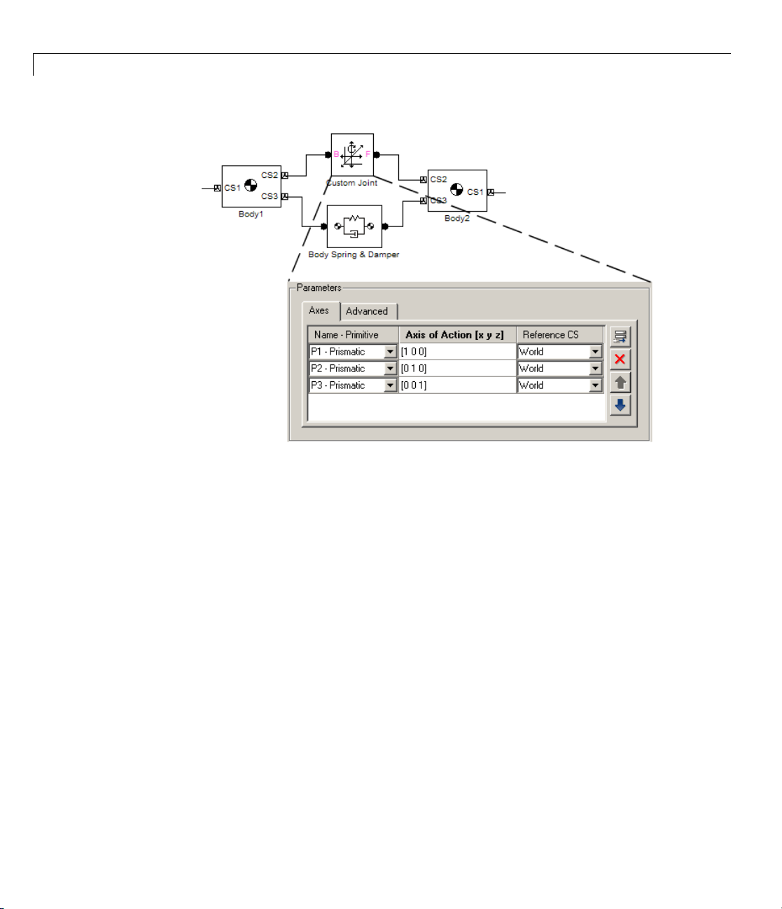
1 Modeling Mechanical Systems

1-76

Inserting a Linear Force or Torque Through a Joint

Another way of inserting a linear force element between two bodies is to connect it to a joint that already connects the bodies. You have to apply the force element, like an actuator, to each primitive in the joint individually. This approach has several advantages over the Body Spring & Damper:

• You can create a different force law, with a different spring length, spring

constant, and damping constant, for each of the joint’s primitives.

• The spring and damper forces acting on each primitive act independently

in their respective directions, instead of depending on just the interbody distance with a single spring length, spring constant, and damping constant.

This allo ws you t o create sprin g and damping forces that act independently in two or three dimensions, unlike the Body Spring & Damper force, which acts only along a single axis. Damping forces acting on multiple primitives act as a two- and three-dimensional viscous medium, not as a dashpot.

• The joint representing the DoFs between the bodies is already present.

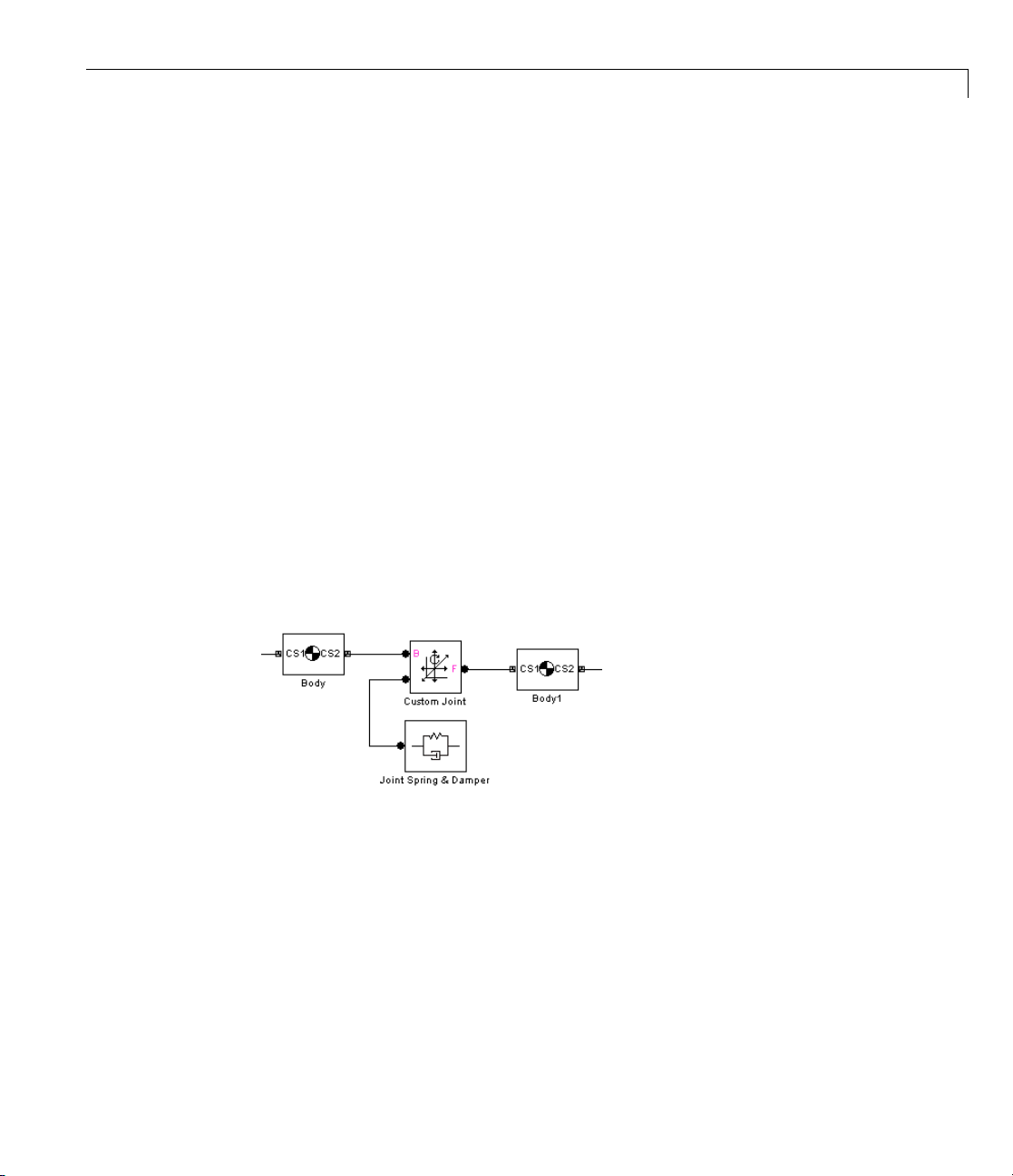
Adding Internal Forces

You use the Joint Spring & Damper block to implement such spring-damper forces/torques together with a Joint. With it, you can apply a linear spring and damper force to each prismatic primitive and a linear torsion and damper torque to each revolute primitive in a Joint block. (You cannot apply these torques to a spherical primitive.)

Pick a Joint already connected between two Bodies. You connect the Joint Spring & Damper block to a Joint block at a sensor/actuator port on the Joint. (The section “Actuating a Joint” on page 1-56 explains how to create such a port.) The Joint Spring & Damper dialog then lists each primitive in t h e Joint.

For each prismatic primitive you want to actuate with a spring-damper force, you specify a natural spring length (offset), spring constant, and damping constant. For each revolute primitive you want to actuate with a torsion-damper torque, you specify a natural torsion angle (offset, or angle in which the primitive points absent any torques), torsion constant, and damping constant. You make these specifications in the Joint Spring & Damper dialog.

Here are two bodies connected by a Custom Joint in turn connected to a Joint Spring & Damper block.

Unlike the example in the preceding section, “Inserting a Linear Force Between Bodies” on page 1-74, the Custom Joint can have up to three prismatics and three revolutes, each with a separate linear force or torque acting through it. Each force or torque acts equally and oppositely on each body, following Newton’s third law.

1-77

1 Modeling Mechanical Systems

Customizing For Feedback

You can create yo by using Sensor only model lin and velocitie

This simple ex Hooke’s law s to its displa

The followi law.

ng SimMechanics model represents a spring that obeys Hooke’s

ur own force elements acting through Joints or on Bodies

-Actuator feedback loops. With this technique, you can not

ear forces, but any force that depends on body or joint positions

ample illustrates the method w ith a linear spring force law.

tates that the force exerted by an extended spring is proportional

cement from its unextended position: F =-kx.

ce Elements with Sensor-Actuator

1-78

The mo displ the sp by the Actu subs

del uses the Gain block labeled Spring Constant to multiply the

acement of the prismatic joint labeled Spring along the World’s y-axis by

ring constant

spring. The model feeds the force back into the prismatic joint via the ator labeled Force. The model encapsulates the spring block diagram in a ystem to clarify the model and to allow a spring to be i nserted elsewhere.

-0.8. The output of the Gain block is the force exerted

Combining One- and Three-Dimensional Mechanical Elements

Combining One- and Three-Dimensional M echanical Elements

In this section...

“About Interface Elements” on page 1-79

“Working with Interface Elements” on page 1-81

“Example: Ro t ati on al Spring-Damper with Hard Stop” on page 1-82

About Inter

SimMechan one-dimen about a sin Simscape and torqu Elements amechan

Consult one-dim

Foundation library include ma sse s , inertias, and internal forces

es, as well as sensors and actuators. The blocks of the Interface

library allow you to selectively couple a SimMechanics machine to

ical circuit.

the Simscape documentation for more about Physical Networks and

ensional domains.

face Elements

ics software is built on the Simscape environment, which supports

sional domains of translational and rotational motion, along or

gle axis for one body at a time. The mechanical elements of the

How Mechanical Inter face Elements Couple Motion and Forces Between SimMechanics Machines and Simscape Circuits

BecauseSimscapemodelssimulatemotion along or about one axis, one Interface Element block can couple only one SimMechanics joint primitive at a time to a Simscape circuit, interfacing through a Sensor/Actuator port on a Joint block. An Interface Element neither adds nor subtracts degrees of freedom (DoFs) to or from the combined machine-mechanical circuit. Its coupling is like a force element between the two domains (see “Adding Internal Forces” on page 1-74):

• From the point of view of the SimMechanics machine, an Interface Element

behaves like a force actuator acting on the selected joint primitive. The interface block injects f orce or torque from the mechanical circuit between the Bodies connected to either side of the Joint.

1-79

1 Modeling Mechanical Systems

• From the point of view of the Simscape mechanical circuit, an Interface

Element behaves like a mo tion actuator. The interface block injects translational or rotational motion from the machine into the circuit connection line.

• The directionality or sense of motion, established by the base (B)-follower

(F) order in the SimMechanics Joint, is preserved in the Simscape mechanical circuit.

• An Interface Element preserves the force or torque flowing through the

Interface Element into the machine and the motion acting across the Joint transmitted into the mechanical circuit. Interface Elements thus conserve mechanical power, transferring it without loss between the two domains.

Interface Elements can couple prismatic or revolute joint primitives to translational or rotational motion, through the Prismatic-Translational Interface o r Revolute-Rotational Interface blocks, respectively.

Limitations on the Inter faced Simscape Mechanical Circuit

SimMechanics and Simscape mechanical simulations are separately valid. However, simulation of moving bodies modeled as Simscape mass and inertia elements coupled through Interface Elements to a SimMechanics machine is not complete and requires care to avoid unphysical results. These limitations arise from their different representations of motion and dynamics coming into conflict:

1-80

• One-dimensional motion in Simscape circuits versus three-dimensional

motion in SimMechanics machines.

A Simscape circuit does not model the motion of such bodies along or about axes orthogonal to the coupled primitiveaxischosenintheinterfacedJoint.

• Absolute motion of each Simscape mass and inertia represented by

connection lines versus relative motion, represented by Joints, between SimMechanics bodies.

All masses in Simscape models live in an implicit inertial reference frame. A Simscape mechanical circuit interfaced to a SimMechanics machine in general moves in an accelerated frame. A simulation wi th such a circuit does not include the pseudoforces acting on the Simscape mass and inertia elements as experienced in such a noninertial frame and thus violates Newton’s second law of mechanics.

Combining One- and Three-Dimensional Mechanical Elements

As the mass and/or inertia modeled in the interfaced mechanical circuit is increased, so is the violation of Newton’ssecondlaw. Assuchmassand/or inertia is decreased, so is the violation.

Warning Model all masses and inertias in your system as Bodies in the SimM echanics machine and avoid placing mass and inertia elements into any interfaced Simscape mechanical circuits.

Models with mass and inertia elements in Simscape mechanical circuits interfaced to a SimMechanics machine are not physically valid. Simulating with such models does not yield valid results.

Working with Interface Elements

To interface a Joint with a Simscape mechanical circuit:

1 Select the appropriate Interface Element block, prismatic or revolute, from

the Interface Elements library.

• Ifyouwishtocoupleatranslational mechanical circuit to a prismatic

primitive, select Prismatic-Translational Interface.

• Ifyouwishtocouplearotationalmechanical circuit to a revolute

primitive, select Revolute-Rotational Interface.

You cannot mix translational and rotational motion with an Interface Element.

2 Copy the selected Interface Element block into your model.

3 Open the Joint dialog and add an extra Sensor/Actuator port. Close the

dialog.

4 Connect the Interface Element mechanical connector port to the new

Sensor/Actuator port on the Joint.

1-81

1 Modeling Mechanical Systems

5 Open the Interface Element dialog. The Connected to primitive

pull-down menu contains a list of all the primitives of appropriate type (prismatic or re vo lute) in the interfaced Joint.

Select the primitive you want to interface. The Simscape circuit will move along or about that axis. Click OK or Apply.

On the machine side, the Joint must follow the standard rules for Joints and in particular be connected to a Body on each side. (See “Modeling Degre es of Freedom” on page 1-19.) You should connect the Interface Element with the rest of the mechanical circuit.

1-82

Example: Rotational Spring-Damper with Hard Stop

The mech_ inte rface_rot_spr_damper demo illustrates proper interface of Simscape mechanical elements with a three-dimensional SimMechanics machine.

Combining One- and Three-Dimensional Mechanical Elements

The interfaced mechanical circuit has no inertia or mass elements, which prevents the problems discussed in “Limitations on the Interfaced Simscape Mechanical Circuit” on page 1-80. It contains only force elements: a rotational spring, a rotational damper, and a rotational hard stop. Together, these force elements create a hard stop for the Revolute block. This block contains only one primitive,

R1, which you can view by opening its dialog. Through

this primitive, the Simscape force elements act between Body A and Body B, limiting their relative angular motion about the revolute

R1 axis to ±π/6

radians.

1-83

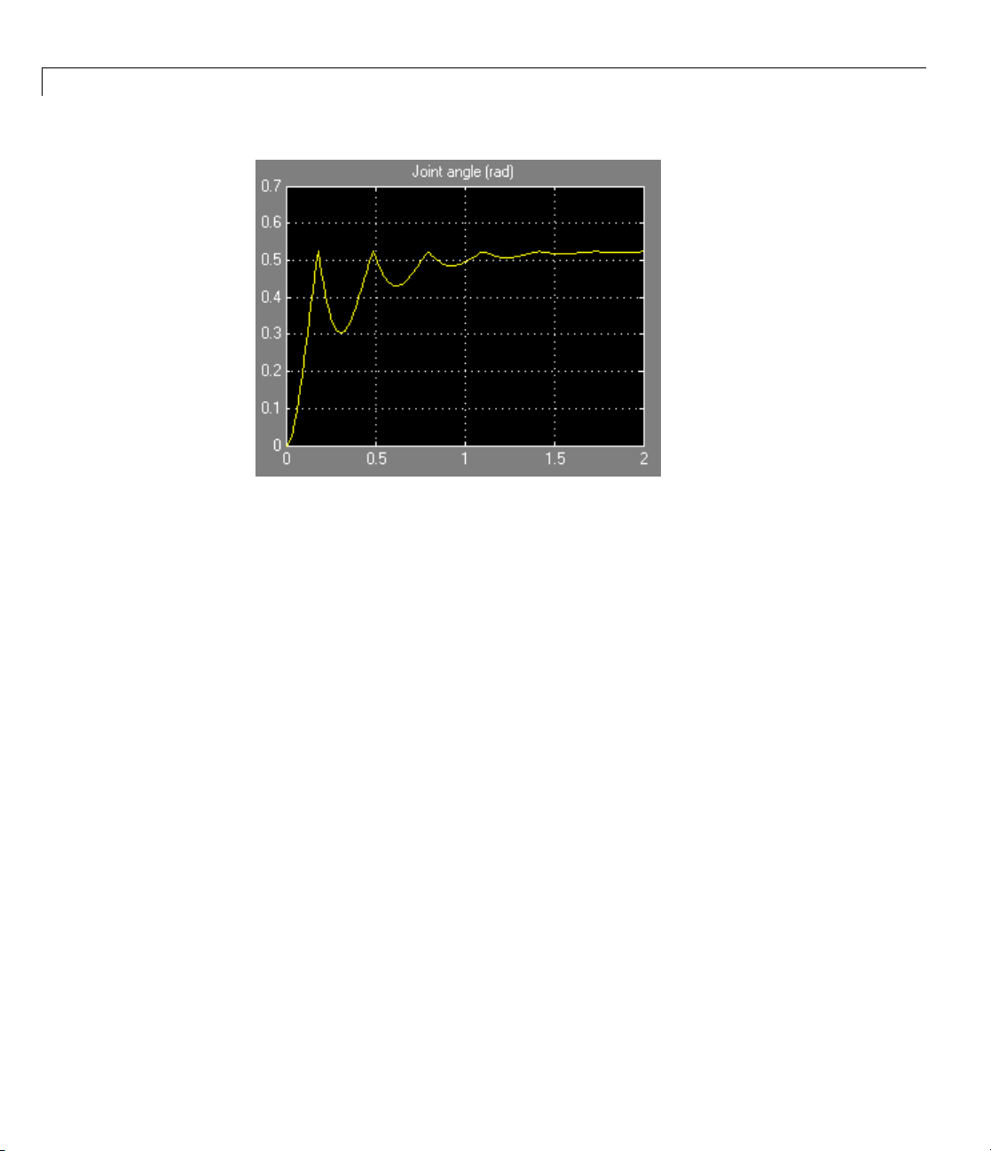
1 Modeling Mechanical Systems

1-84

Validating Mechanical Models

In this section...

“Essential Tests for Model Validity” on page 1-85

“Verifying Model Topology” on page 1-85

“Counting Model Degrees of Freedom” on page 1-89

Essential Tests for Model Validity

Simulink can simulate a SimMechanics model only if it is valid. A model is valid if it satisfies the following rules:

• Each machine in the model contains at least one Ground, and exactly one

Ground in each machine is connected to a Machine Environment block. Each submachine connected to a full machine by a Shared Environment block must have at least one Ground.

See “Representing Machines with Models” on page 1-2.

Validating Mechanical Models

• Every machine in the model is topologically valid. See “Verifying Model

Topology” on page 1-85.

• The model contains at least one degree of freedom. See “Counting Model

Degrees of F reedom” on page 1-89.

• Any machine in the model interfaced to Simscape mechanical circuits

satisfies both SimMechanics and Simscape modeling rules. See “Combining One- and Three-Dimensional Mechanical Elements” on page 1-79.

Verifying Model Topology

To avoid simulation failures, you must ensure that the topology of your block diagram is valid. A block diagram is topologically valid if each machine that it contains is valid. A machine is valid if its spanning tree is valid. Th us to determine if your model is valid, first determine the spanning tree of each machine that it contains and then the validity of each resulting tree.

1-85

1 Modeling Mechanical Systems

Machine Topology and Subsystems

When examining your model’s topology, be sure to inspect all its subsystems, including m asked subsystems, down to the bottom of the model’s subsystem hierarchy.

Determining a Mach ine’s Spanning Tree

You can think of a machine as a graph with elements (bodie s) and connectors (joints, constraints, and drivers). A spanning tree is a reduced graph with bodies connected only by joints and all closed loops cut once.

To determine the spanning tree of a machine, remove all blocks from the machine except Body and Joint blocks and open every closed loop in the resulting reduced machine. To open a closed loop, follow the loop-cutting rules in “Cutting Machine Diagram Loops” on page 1-46.

For example, here is a machine with two closed loops.

1-86

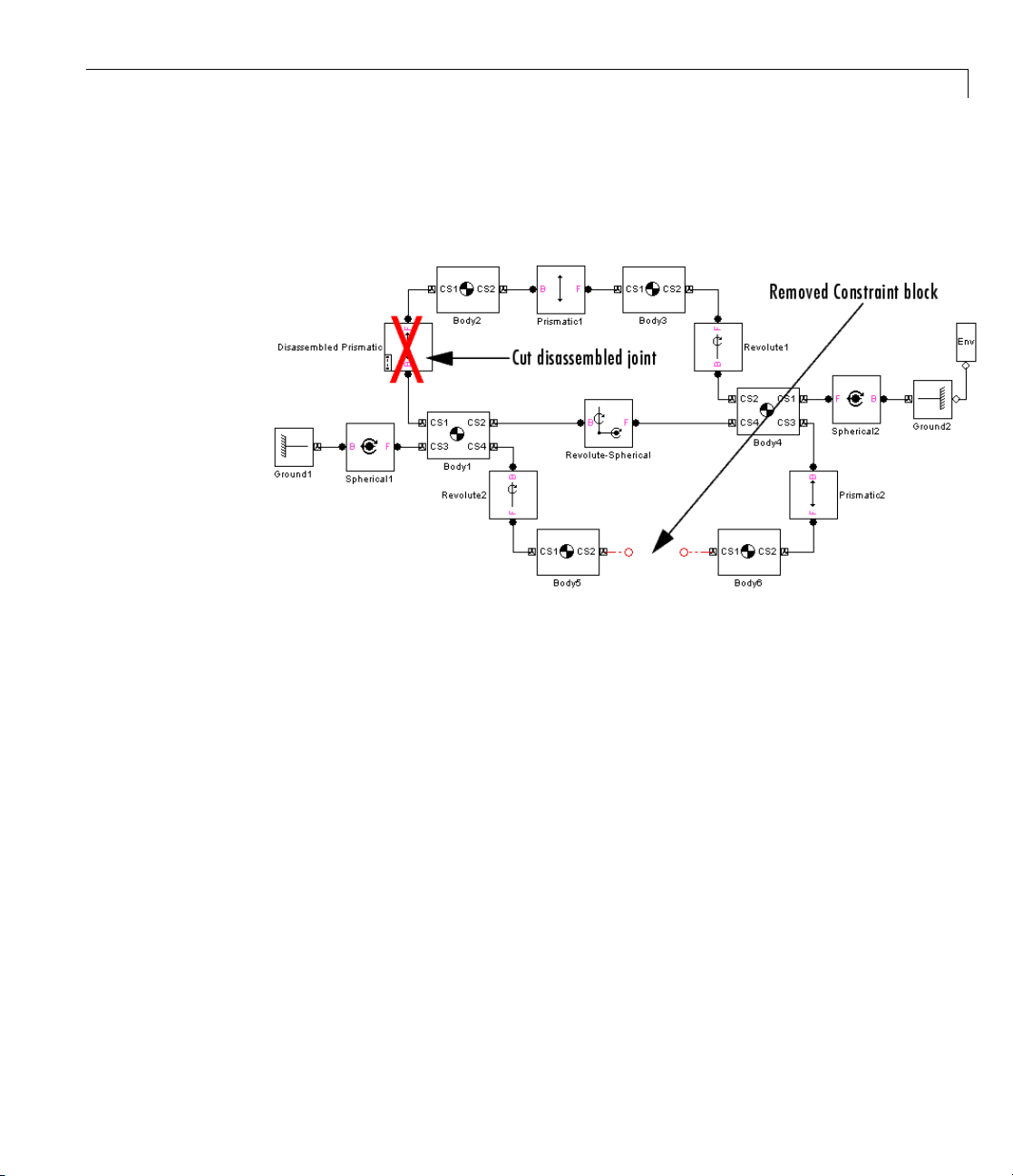
Validating Mechanical Models

CuttingthetoploopattheDisassembledPrismaticandremovingtheParallel Constraint block (thus simultaneously cutting the bottom loop) yields the machine’s spanning tree, as shown here.

Determining the Validity of a Spanning Tree

To be valid, a spanning tree must meet these requirements:

• ThespanningtreemusthaveatleastoneGroundblocktoserveasa

reference to World.

• Every Joint block must be connected to exactly two Body blocks.

• Every non-Ground Body block must have a unique path to a Ground block.

(This need not be true of the whole machine.) This ensures that, while each body moves via joints relative to other bodies, the simulation can resolve all bodies’ motions relative to one another into absolute motions with respect to World.

• Every non-Ground Body block at an end of a chain of Bodies must have

nonzero inertia (mass or inertial moment) associated with all joint primitives that can move. Each translational DoF must carry a nonzero mass, and each rotational DoF a nonzero inertial moment. This prevents infinite accelerations when forces and torques are applied.

1-87

1 Modeling Mechanical Systems

Examples of Invalid Machine Topologies

Herearesomeexamplesofinvalidtopologies:

• This one-loop machine lacks a Ground block.

• This open machine has a dangling Joint block.

1-88

Mathworks SIMMECHANICS 3 user guide

Specifications and Main Features

Frequently Asked Questions

User Manual

Modeling Mechanical Systems

Representing Machines with Models

About Machines

About SimMechanics Models

Creating a SimMechanics Model

Connection Lines

Connector Ports

Creating SimMechanics Subsystems

Creating a Subsystem Automatically

Modeling Grounds and Bodies

About Bodies and Grounds

Modeling Grounds

Machine Environment Required for Each Machine

World and Grounded Coordinate Systems

Modeling Rigid Bodies

About Body Blocks

Creating a Body Block

Determining Inertia Tensors for Common Shapes

Working with Body Coordinate Systems

Setting a Body CS’s Position

Managing Body Coordinate Systems

Creating Body CS Ports

Modeling Degrees of Freedom

About Joints

Modeling Joints

Joint Primitives

Joint Types

Joint Axes

Joint Directionality

Assembly Restrictions

Creating a Joint

Directing Joint Axes

Assembling Joints

Creating a Massless Connector

Massless Connector Example: Triple Pendulum

Massless Connector Example: Four Bar Mechanism

Modeling Disassembled Joints

Controlling Automatic Assembly and the Assembled Configuration

Disassembled Joint Example: Four Bar Mechanism

Constraining and Driving Degrees of Freedom

About Constraints

TypesofMechanicalConstraints

What Constraints and Drivers Do

Directionality of Constraints and Drivers

Solving Constraints

Mitigating Constraint Singularities

Visualizing the Gear Motion

Driver Example: Angle Driver

The Angle Driver Without a Driver Actuator

Visualizing the Angle Driver Motion

The Angle Driver With a Driver Actuator

Cutting Machine Diagram Loops

Rules for Valid Machine Diagram Loops

Rules for Automatic Loop Cutting

Specifying a Loop Joint for Cutting

Displaying the Cut Joints

For More About Disassembled and Cut Joints

For More About Constraints and Drivers

Applying Motions and Forces

About Actuators

Stabilizing Numerical Derivatives in Actuator Signals

Examples of Numerical Deriv atives of Actuator Signals

Actuating a Body

Body Actuator Example: Pure Kinetic Friction

Applying Motions to Bodies

Example: Simple Rocket

Actuating a Joint

Actuating a Joint Primitive

Joint Actuator Example: Body Driver

Actuating a Driver

Specifying Initial Positions and Velocities

Using JICA Blocks

JICA Example: A Simple Pendulum

Sensing Motions and Forces

About Sensors

Home Configuration and Position-Orientation Measurements