Mathworks SIMHYDRAULICS 1 user guide

Download

SimHydraulics

User’s Guide

How to Contact The MathWorks

www.mathworks. comp.soft-sys.matlab Newsgroup www.mathworks.com/contact_TS.html Technical Support

suggest@mathworks.com Product enhancement suggestions

bugs@mathwo doc@mathworks.com Documentation error reports service@mathworks.com Order status, license renewals, passcodes

info@mathwo

com

rks.com

Web

Bug reports

Sales, prici

ng, and general information

508-647-7000 (Phone)

508-647-7001 (Fax)

The MathWorks, Inc. 3 Apple Hill Drive Natick, MA 01760-2098

For contact information about worldwide offices, see the MathWorks Web site.

SimHydraulics

The software described in this document is furnished under a license agreement. The software may be used or copied only under the terms of the license agreement. No part of this manual may be photocopied or reproduced in any form without prior written consent from The MathW orks, Inc.

FEDERAL ACQUISITION: This provision applies to all acquisitions of the Program and Documentation by, for, or through the federal government of the United States. By accepting delivery of the Program or Documentation, the government hereby agrees that this software or documentation qualifies as commercial computer software or commercial computer software documentation as such terms are used or defined in FAR 12.212, DFARS Part 227.72, and DFARS 252.227-7014. Accordingly, the terms and conditions of this Agreement and only those rights specified in this Agreement, shall pertain to and govern theuse,modification,reproduction,release,performance,display,anddisclosureoftheProgramand Documentation by the federal government (or other entity acquiring for or through the federal government) and shall supersede any conflicting contractual terms or conditions. If this License fails to meet the government’s needs or is inconsistent in any respect with federal procurement law, the government agrees to return the Program and Docu mentation, unused, to The MathWorks, Inc.

Trademarks

MATLAB and Simulink are registered trademarks of The MathWorks, Inc. See

www.mathworks.com/trademarks for a list of additional trademarks. Other product or brand

names may be trademarks or registered trademarks of their respective holders.

Patents

The MathWorks products are protected by one or more U.S. patents. Please see

www.mathworks.com/patents for more information.

User’s Guide

Revision History

March 2006 Online only New for Version 1.0 (Release 2006a+) September 2006 O nline only Revised for Version 1.1 (Release 2006b) March 2007 Online only Revised for Version 1.2 (Release 2007a) September 2007 O nline only Revised for Version 1.2.1 (Release 2007b) March 2008 Online only Revised for Version 1.3 (Release 2008a) October 2008 Online only Revised for Version 1.4 (Release 2008b) March 2009 Online only Revised for Version 1.5 (Release 2009a) September 2009 O nline only Revised for Version 1.6 (Release 2009b) March 2010 Online only Revised for Version 1.7 (Release 2010a)

Getting Started

Product Overview ................................. 1-2

Product Description Assumptions and Limitations The Physical Modeling Product Family Getting Online Help

............................... 1-2

....................... 1-2

................ 1-3

............................... 1-3

Contents

Getting Started

• “Product Overview” on page 1-2

• “Related Products” on page 1-5

• “Modeling Physical Networks with S imHydraulics Blocks” on page 1-6

• “Running Hydraulic Models” on page 1-7

• “Troubleshooting Hydraulic Models” on page 1-8

• “Using Simscape E diting Modes” on page 1-10

1 Getting Started

Product Overview

Product Description

SimHydraulics®software is a modeling environment for the engineering design and simulation of hydraulic power and control systems within Simulink the Simscape™ modeling environment and contains a comprehensive library of hydraulic blocks tha t extends the Simscape libraries of basic hydraulic, electrical, and one-dimensional translational and rotational mechanical elements and utility blocks.

In this section...

“Product Description” on page 1-2

“Assumptions and Limitations” on page 1-2

“The Physical Modeling Product Family” on page 1-3

“Getting Online Help” on page 1-3

and MATLAB®. It is based on the Physical Network approach of

1-2

Assumptions and Limitations

SimHydraulics software performs transient analysis of hydro-mechanical systems. You may be able to use the higher-level library blocks, or you may need to build your actuators out of the lower-level library blocks. SimHydraulics software is specifically developed to cover modeling scenarios with hydraulic actuators as part of a control system. It is also appropriate for systems that allow consideration in lumped parameters.

SimHydraulics software does not have the capability to model the followin g types of systems:

• Fluid transportation

• Water supply and sewer systems

• Distributed parameters systems

Product Overview

SimHydraulics software is based on the assumption that fluid temperature remains constant during the simulated time interval, and this temperature must be set as a parameter together with the relative amount of entrapped air.

ThePhysicalModelingProductFamily

SimHydraulics software is based on the Simscape platform product for the Simulink Physical Modeling family, encompassing the modeling and design of systems according to basic physical principles. Simscape software runs within the Simulink e nvironment and interfaces seamlessly with the rest of the Sim ulink and MATLAB product families. Unlike other Simulink blocks, which represent mathematical operations or operate on signals, Simscape blocks represent physical components or relationships directly.

Note This SimHydraulics User’s Guide assumes that you have some experience with modeling hydraulic systems, as well as with building and running models in the Simulink environment.

Getting Online Help

Using the MATLAB Help System for Documentation and Demos

TheMATLABHelpbrowserallowsyoutoaccessthedocumentationanddemo models for all the MATLAB and Simulink based products that you have installed. Consult “Overview of Help” in MATLAB documentation for more information about the Help system.

For...

List of blocks “Block Reference”

Advanced tutorials

Product demonstrations

What’s new in this product

See...

Examples

SimHydraulics Demos

Release Notes

1-3

1 Getting Started

The MathWorks Online

Point your Internet brow ser to the MathWorks Web site for additional information and support at http://www.mathworks.com/products/simhydraulics/.

1-4

Related Products

In this section...

“Product Requirements” on page 1-5

“Other Related Products” on page 1-5

Product Requirements

SimHydraulics software is the extension of Simscape platform product, expanding its capabilities to model and simulate hydraulic elements and devices.

SimHydraulics software requires these products:

• MATLAB

• Simulink

• Simscape

Other Related Products

The related products listed in the SimHydraulics product page a t the MathWorks Web site include toolboxes and blocksets that extend the capabilities of MATLAB and Simulink. These products will enhance your use of SimHydraulics software in various applications.

For more information about The MathWorks™ software products, see either

• The online documentation for that product if it is installed

• The MathWorks Web site at

www.mathworks.com

1-5

1 Getting Started

Modeling Physical Networks with SimHydraulics Blocks

Simscape modeling environment provides the Physical Network approach for modeling and solving systems under design as one-dimensional networks. SimHydraulics software utilizes these basic modeling principles and contains a library of specialized hydraulic blocks that seamlessly interact with basic Simscape blocks.

SimHydraulics models are essentially Simscape block diagrams. When building a S imHydraulics model, you use a combination of SimHydraulics blocks with the blocks from the Simscape Foundation and Utilities libraries. Each SimHydraulics diagram must have at least one Solver Configuration block from the Simscape Utilities library. You can use basic hydraulic, electrical, and one-dimensional translational and rotational mechanical elements from the Simscape Foundation library and directly connect them to SimHydraulics blocks. You can also use basic Simulink blocks, such as sources and scopes, but you need to connect them through the Simulink-PS Converter and P S-Simulink Converter blocks from the Simscape Utilities library. You can also use these converter blocks to specify the desired input and output signal units. For more information on specifying units in SimHydraulics diagrams, see “Working with Physical Un its” in the Simscape documentation.

1-6

General rules that you must follow when building a hydraulic model are described in “Basic Principles of Modeling Physical Networks” in the Simscape documentation. Chapter 2, “Modeling Hydraulic Systems” in this SimHydraulics User’s Guide briefly reviews these rules and provides specific examples of modeling hydraulic systems and their components, such as power units and directional valves.

Running Hydraulic Models

SimHydraulics software gives you multiple ways to simulate and analyze hydraulic power and control systems in the Simulink environment. Running a hydraulic simulation is similar to running a simulation of any other Simscape model. See “Simulating Physical Models” in the Simscape documentation for a discussion of the following topics:

• Explanation of how SimHydraulics software validates and simulates a

model

• Specifics of using Simulink linearization commands in SimHydraulics

models

• Generating code for SimHydraulics models

• Restrictions and limitations on using Simulink tools in SimHydraulics

models

All th ese aspects of simulating SimHydraulics models are exactly the same as for Simscape models.

Running Hydraulic Models

1-7

1 Getting Started

Troubleshooting Hydraulic Models

SimHydraulics simulations can stop before completion with one or more error messages. For a discussion of generic error types and error-fixing strategies, see “Troublesho oting Simulation Errors” in the Simscape documentation. The following troubleshooting techniquesarespecifictohydraulicmodels:

• Review the model configuration. If your error message contains a list of

blocks, look at these blocks first. Also look for:

- Wrong connections — Verify that the model makes sense as a hydraulic

system. For example, look for accumulators connected to the pump outlet without check valves; cy linde rs connected against each other, so that they try to move in opposite directions; directional valv es bypassed by a huge orifice, and so on.

- Wronguseofhydraulicelements—SimHydraulicsblocksmodeltheir

respective hydraulic units within certain limits. For example, an Ideal Pressure Source block can simulate a pump only when the pressure remains constant (see “Modeling Power Units” on page 2-27). Similarly, the P ressu re Relief Valve block is a steady-state representation of a real valve. A block may exhibit wrong behavior if it is placed in the wrong environment. Always check the va lidity of the model for a particular environment and the simulation objectives.

1-8

• Avoid portions of the system getting isolated from the main system.

An isolated or "hanging" part of the system could affect computational efficiency and even cause failure of computation. Use the Leakage Area parameter, introduced specifically for this purpose, to maintain numerical integrity of the circuit. This parameter is pres ent in all the directional valve blocks, pressure control and flow control valve blocks, and most of the variable orifices.

• Avoid "dry" nodes in a hydraulic system. By adding a hydraulic chamber to

a node, you can considerably improve the convergence and computational efficiency of a model. Mathematically, the hydraulic chamber works in approximately the same way a s mechanical inertia does in mechanical systems. The hydraulic chamber is represented by the Constant Volume Hydraulic Chamber block in the Simscape Hydraulic Elements library.

The MathWorks recommends that you build, simu la te, and test your model incrementally. Start with an idealized, simplified model of your

Troubleshooting Hydraulic Mod els

system, simulate it, verify that it works the way you expected. Then incrementally make your model more realistic, factoring in effects such as fluid compressibility, fluid inertia, and the other things that describe real-world phenomena. Simulate and test your model at every incremental step. Use subsystems to capture the model hierarchy, and simulate and test your subsystems separately before testing the whole model configuratio n. This approach helps you keep your models well organized and makes it easier to troubleshoot them.

1-9

1 Getting Started

Using Simscape Editing Modes

The Simscape Editing Mode functionality lets you open, simulate, and save models that contain blocks from add-on products, including SimHydraulics blocks, in Restricted mode, without checking out add-on product licenses, as long as the products are installed on your machine.

This functionality allows a user, model developer, to build a model that uses Simscape and SimHydraulics blocks and share that model with other users, model users. When building the model in Full mode, the model developer must have both a Simscape license and a SimHydraulics license. Once the model is built, model users need only to check out a Simscape license to simulate the model and fine-tune its parameters in Restricted mode. As long as no structural changes are made to the model, model users can work in Restricted mode and do not need to check out SimHydraulics licenses.

Another workflow lets multiple users, who all have Simscape licenses, share a small number of SimHydraulics licenses by working mostly in Res tricted mode, and temporarily switching models to Full mode only when they need to perform a specific design task that requires being in Full mode.

1-10

For a complete description of this functionality, see “Using the Simscape Editing Mode” in the Simscape documentation.

Modeling Hydraulic Systems

• “Introducing the SimHydraulics Block Libraries” on page 2-2

• “Essential Steps to Building a Hydraulic Model” on page 2-5

• “Creating a Simple Model” on page 2-8

• “Modeling Power Units” on page 2-27

• “Modeling Directional Valves” on page 2-31

• “Modeling Low-Pressure Fluid TransportationSystems”onpage2-45

2 Modeling Hydraulic Systems

Introducing the SimHydraulics Block Libraries

In this section...

“Library Structure Overview” on page 2-2

“Using the Simulink Library Browser to Access the Block Libraries” on page 2-2

“Using the Command Prompt to Access the Block Libraries” on page 2-4

Library Structure Overview

SimHydraulicssoftwareusestheSimscape library as its main library. Simscape modeling environment provides the Physical Network approach for modeling and solving systems under design as one-dimensional networks. SimHydraulics software utilizes these basic modeling principles and contains a library of specialized hydraulic blocks that seamlessly interact with basic Simscape blocks. When modeling hydraulic power and control systems, you use the following Simscape libraries:

2-2

• Foundatio n library — Contains basic hydraulic, mechanical, and physical

signal blocks

• SimHydraulics library — Contains advanced hydraulic diagram blocks,

such as valves, cylinders, pipelines, pumps, and accumulators

• Utilities library — Contains essential environment blocks for creating

Physical Networks models

You can combine all these blocks in your SimHydraulics diagrams to model hydraulic systems. You can also use the basic Simulink blocks in your diagrams, s uch as sources or scopes. See“ConnectingSimscapeDiagramsto Simulink Sources and Scopes” for more information on how to do this.

Using the Simulink Library Browser to Access the Block Libraries

You can access the blocks through the Simulink Library Browser. To display the Library Browser, click the Library Browser button in the toolbar of the MATLAB desktop or Simulink model window:

Introducing the SimHydraulics®Block Libraries

Alternatively, you can type simulink in the MATLAB Command Window. Then expand the Simscape entry in the contents tree.

For more information on using the Library Brow ser, see “Library Browser” in the Simulink Graphical User Interface documentation.

2-3

2 Modeling Hydraulic Systems

Using the Comman Libraries

Another way to ac using the comm a

• To open just th

Command Windo

• To open the Si

hydraulic s o

simscape in t

• To open the m

simulink in

The SimHyd in the foll sublibrar more deta “Block Re

owing illustration. Some of these libraries contain second-level

ies. You can expand each library by double-clicking its icon. For

ils on library hierarchy and descriptions of block categories, see

ference”.

cess the block libraries is to open them individually by

nd prompt:

e SimHydraulics library, type

mscape library (to access the utility blocks, as w ell as

urces, sensors, and other Foundation library blocks), type

he MATLAB Command Window.

ain Simu link library (to access generic Simulink blocks), type

the MATLAB Command Window.

raulics library consists of eight top-level libraries, as shown

d Prompt to Access the Block

sh_lib in the MATLAB

2-4

Essential Steps to Building a Hydraulic Model

In this section...

“Overview of Modeling Rules” on page 2-5

“Working with Fluids” on page 2-6

Overview of Modeling Rules

The rules that you must follow when building a hydraulic model are described in “Basic Principles of Modeling Physical Network s ” in the Sims ca pe documentation. This section briefly reviews these rules.

• SimHydraulics blocks, in general, feature C onserving ports

Signal inports and outports

• There are three types of Physical Conserving ports used in SimHydraulics

blocks: hydraulic, mechanical translational, and mechanical rotational. Each type has specific Through and Across variables associated with it.

• You can connect Conserving ports only to other Conserving ports of the

same type.

• The Physical connection lines that connect Conserving ports together

are bidirectional lines that carry physical variables (Across and Through variables, as described above) rather than signals. You cannot connect Physical lines to Simulink ports or to Physical Signal ports.

• Two directly connected Conserving ports must have the same values for all

their A cross variables (such as pressure or angular velocity).

• You can branch Physical connection lines. When you do so, components

directly connected with one another continue to share the same Across variables. Any Through variable (such as flow rate or torque) transferred along the Physical connection line is divided among the multiple components connected by the branches. How the Through variable is divided is determined by the system dynamics.

For each Through variable, the sum of all its values flowing into a branch point equals the sum of all its values flowing out.

and P h ysical

2-5

2 Modeling Hydraulic Systems

• You can connect Physical Signal ports to other Physical Signal ports with

• You can connect Physical Signal ports to Simulink ports through special

• Unlike Simulink signals, which are essentially unitless, Physical Signals

For examples of applying these rules w hen creating an actual hydraulic model,see“CreatingaSimpleModel”onpage2-8.

The MathWorks recommends that you build, simulate, and test your model incrementally. Start with an idealized, simplified model of your system, simulate it, verify that it works the way you expected. Then incrementally make your model more realistic, factoring in effects such as friction loss, motor shaft compliance, hard stops , and the other things that describe real-world phenomena. Simulate and test your model at every incremental step. Use subsystems to capture the model hierarchy, and simulate and test your subsystems separately before testing the whole model configuratio n. This approach helps you keep your models well organized and makes it easier to troubleshoot them.

regular connection lines, similar to Simulink signal connections. These connection lines carry physical signals betw een SimHydraulics blocks.

converter blocks. Use the Simulink-PS Converter block to connect Simulink outports to Physical Signal inports. Use the PS-Simulink C onverter block to connect Physical Signal outports to Simulink inports.

can h ave units ass ociated with them. SimHydraulics block dialogs let you specify the units along with the param eter values, where appropriate. Use the converter blocks to associate units with an input signal and to specify the desired output signal units.

2-6

Working with Fluids

A change in the working fluid of your SimHydraulics model affects the global parameters of the system. Global parameters, determined by the type of working fluid, are used in equations for most hydraulic blocks. For example, valves, orifices, and pipelines use fluid density and fluid kinematic viscosity; chambers and cylinders use fluid bulk modulus; and so on. When you change the type of fluid, the appropriate changes to the global parameter values are propagated to all the blocks in the hydraulic circuit.

Essential Steps to Building a Hydraulic Model

Each topologically distinct hydraulic circuit in a diagram requires exactly one hydraulic fluid to be associated with it. You can specify the fluid by connecting a Hydraulic Fluid block or Custom Hydraulic Fluid block to the circuit.

• The Custom Hydraulic Flu i d block, available i n the Simscape Foundation

library, lets you directly specify the fluid properties, such as fluid density, kinematic viscosity, bulk modulus, and the amount of entrapped air, in the block dialog.

• The Hydraulic Fluid block lets you select a type of fluid from a predefined

list and specify the amount of entrapped air and fluid temperature. SimHydraulics software determines the fluid properties associated with this type of fluid and these conditions, and displays them in the block dialog.

In both cases, SimHydraulics software then applies the fluid properties as global parameters to all the blocks in the hydraulic circuit.

Note If no Hydraulic Fluid block or Custom Hydraulic Fluid block is attached to a circuit, the hydraulic blocks in this circuit use the default fluid, which is Skydrol LD-4 at 60°C and with a 0.005 ratio of entrapped air. See the Hydraulic Fluid block reference page for more information.

2-7

2 Modeling Hydraulic Systems

Creating a Simple Model

In this section...

“Building a SimHydraulics Diagram” on page 2-8

“Modifying Initial Settings” on page 2-16

“Running the Simulation” on page 2-20

“Adjusting the Parameters” on page 2-22

Building a SimHydraulics Diagram

In this example, you are going to model a simple hydraulic system and observe its behavior under various conditions. This tutorial illustrate s the essential steps to building a hydraulic model, described in the previous section, and makes you familiar with using the basic SimHydraulics blocks.

The following schematic represents the model you are about to build. It contains a single-acting hydraulic cylinder, which is controlled by an electrically operated 3-way directional valve. The cylinder drives a load consisting of a mass, viscous friction, and preloaded spring.

2-8

Creating a Simple Model

The power unit consists of a motor, a positive-displacement pump, and a pressure relief valve. Depending on its characteristics, such a power unit can be modeled in a variety of ways, as described in “Modeling Power Units” on page 2-27. In this example, the pump unit is assumed to be powerful enough to maintain constant pressure at the valve inlet. Therefore, we are going to representitinthediagrambyaHydraulic Pressure Source block.

To create an equivalent SimHydraulics diagram, follow these steps:

1 Open the Simscape and Simulink block libraries, as described in

“Introducing the SimHydraulics Block Libraries” on page 2-2.

2 Create a new m odel. To do this, click the New button on the Library

Browser’s toolbar or choose New from the library window’s File menu and select Model. The software creates an empty model in memory and displays it in a new model editor window.

Note Alternately, you can type ssc_new at the MATLAB Command prompt, to create a new model prepopulated with certain required and commonly-used blocks. For more information, see “Creating a New Simscape Model”.

3 Open the Simscape > Foundation Library > Hydraulic > Hydraulic Sources

library and drag the Hydraulic Pressure Source block into the model window.

4 OpentheSimscape>SimHydraulics>Hydraulic Cylinders library and

place the Single-Acting Hydraulic Cylinder block into the model window.

5 To model the valve, open the Simscape > SimHydraulics > Valves library.

Place the 3-Way Directional Valve block, found in the Directional Valves sublibrary, a nd the 2-Position Valve Actuator block, found in the Valve Actuators sublibrary, into the model window.

2-9

2 Modeling Hydraulic Systems

6 Connect the blocks as shown in the following illustration.

2-10

Creating a Simple Model

7 Ports T of the Hydraulic Pressure Source and 3-Way Directional Valve

blocks have to be connected to the tank, at atmospheric pressure. To model this connection, open the Simscape > Foundation Library > Hydraulic > Hydraulic Elements library and add the Hydraulic Reference block to your diagram, as shown below. To do this, connect the only port of the Hydraulic Reference block to port T of the Hydraulic Pressure Source block, then right-click this connection line to create a branching point, and connect this point to port T of the 3-Way Directional Valve block.

2-11

2 Modeling Hydraulic Systems

8 Model the mechanical load for the cylinder. Open the Simscape >

Foundation Library > Mechanical > Translational Elements library and add the Mass, Translational Spring, Translational Damper, and three Mechanical Translational Reference blocks to your diagram.

To indicate that the cylinder case is fixed, connect port C of the Single-Acting Hydraulic Cylinder block to one of the Mechanical Translational Reference blocks. To rotate the Mechanical Translational Reference block, select it and press Ctrl+R. You can also shorten the block nametoMTRtomakethediagrameasiertoread.

Connect the other blocks to port R of the Single-Acting Hydraulic Cylinder block, as shown below .

2-12

Creating a Simple Model

9 Now you need to add the sources and scopes. They are found in the regular

Simulink libraries. Open the Simulink > Sources library and copy the Constant block and the Sine Wave block into the model. Then open the Simulink > Sinks library and copy two Scope blocks. Rename one of the Scope blocks to

Valve. It will monitor the valve opening based on the input

signal variation. The other Scope block will monitor the position of the cylinder rod; rename it to

Position.

2-13

2 Modeling Hydraulic Systems

10 Double-click the Valve scopetoopenit. Inthescopewindow,click to

11 Every time you connect a Simulink source or scope to a SimHydraulics

access the scope parameters, change Number of axes to The scope window now displays two sets of axes, and the the diagram has two input ports.

diagram, you have to use an appropriate converter block, to conve rt Simulink signals into physical signals and vice versa. Open the Simscape > Utilities library and copy two Simulink-PS Converter blocks and two PS-Simulink Converter blocks into the model. Connect the blocks as shown below.

2,andclickOK. Valve scope in

2-14

Creating a Simple Model

12 To specify the fluid propertie s, add the Hydraulic Fluid block, found in the

Simscape > SimHydraulics > Hydraulic Utilities library, to your diagram. You can add this block anywhere on the hydraulic circuit by creating a branching point and connecting it to the only port of the Hydraulic Fluid block.

13 Each topologically distinct physical network in a diagram requires exactly

one Solver Configuration block, found in the Simscape > Utilities library. Copy this block into your model and connect it to the circuit, similar to the Hydraulic Fluid block. Your diagram now should look like this.

14 Your block diagram is now complete. Save it as simple_hydro1. mdl.

2-15

2 Modeling Hydraulic Systems

Modifying Initial Settings

After you have put together a block diagram of your model, as described in the previous sectio n, you nee d to select a solver and provide the correct values for block parameters. All the blocks have default parameter values that allow them to run “out of the box,” but you may need to change some of them to suit your particular application.

To prepare for simulating the model, follow these steps:

1 Select a Simulink solver. On the top menu bar of the model window,

select Simulation > Configuration Parameters. The Configuration Parameters dialog box o pens, showing the Solver node.

Under Solver options,setSolver to size to

Also note that Simulation time is specified to be between 0 and 10 seconds. You can adjust this setting later, if needed.

0.2.

ode15s (Stiff/NDF) and Max step

2-16

Creating a Simple Model

Click OK to close the Configuration Parameters dialog box.

2 Select a fluid. Double-click the Hydraulic Fluid block. In the Block

Parameters dialog box, set Hydraulic Fluid to

Skydrol 5 and set the

other block parameters as shown below.

2-17

2 Modeling Hydraulic Systems

2-18

Click OK to close the Block Parameters dialog box.

3 Specify the units for the pressure input signal. Simulink signals are

unitless. When you conv ert them to physical signals, you can supply units by using the converter blocks. Double-click the Simulink-PS Converter1 block, enter

Pa in the Input signal unit combo box, and click OK.When

the physical modeling software parses the model, it matches the input signal units with the block input ports and provides error messages if there is a discrepancy. For more information, see “Model Validation”.

4 Specify a realistic value for the pressure input signal. Double-click the

Constant block, enter

5 Open the 2-Position Valve Actuator block and note that its Nominal

Signal Value parameter is set to

10e5 in the Constant value text box, and click OK.

24.

Creating a Simple Model

6 Double-clicktheSineWaveblockandchangeitsAmplitude to a value

greater than 50% of the nominal signal value for the 2-Position Valve Actuator block, for example, to

7 Adjust the 3-Way Directional Valve block parameters as shown below.

20.

8 Adjust the Single-Acting Hydraulic Cylinder block parameters as shown

below.

2-19

2 Modeling Hydraulic Systems

2-20

9 Double-click the Mass block and change its Mass to 4.5 kg.

10 Doubl

11 Double-click the Translational Spring block. Set its Spring rate to 6e3

12 Save the model.

e-click the Translational Damper block, which models the viscous

ion, and change its Damping coefficient to

frict

and Initial deformation to 0.02 m.

N/m

250 N/(m/s).

Running the Simulation

After you’ve put together a block diagram and specified the initial settings for your model, you can run the simulation.

Creating a Simple Model

1 The input signal for the valve opening isprovidedbytheSineWaveblock.

The Valve scope reflects both the in put signal and the valve opening as functions of time. The Position scope outputs the cylinder rod displacement as a function of time. Double-click both scopes to open them.

2 To run the simulation, click in the model window toolbar. The physical

modeling solver evaluates the model, calculates the initial conditions, and runs the simulation. For a detailed description of this process, see “How Simscape Simulation Works”. Completion of this step may take a few seconds. The message in the bottom-left corner of the model window provides the status update.

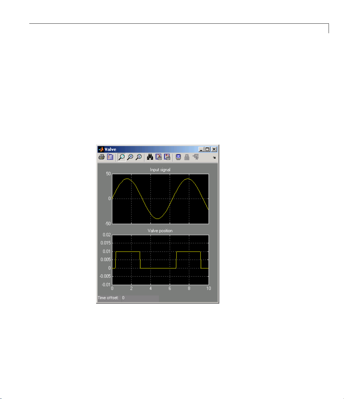
3 Once the simulation starts running, the Valve and Position scope windows

display the simulation results, as showninthenextillustration.

2-21

2 Modeling Hydraulic Systems

In the beginning, the valve is closed. Then, as the input signal reaches 50% of the actuator’s nominal signal, the valve gradually opens t o its maximum value and moves the cylinder rod in the positive direction. W hen the input signal goes below 50% of the nominal signal, the actuator closes the valve. The spring returns the cylinder rod to its initial position.

2-22

You can now adjust various inputs and block parameters and see their effect on the valve opening profile and the cylinder rod displacement.

Adjusting the Parameters

After running the initial simulation, you can experiment with adjusting various inputs and block parameters.

Try the following adjustments:

1 Change the input signal for valve opening.

2 Change the cylinder load parameters.

3 Change the rod position output units.

Creating a Simple Model

Changing the Valve Input Signal

This example shows how a change in the input signal affects the opening of the valve, and therefore the cylinder rod displacement.

1 Double-clicktheSineWaveblock,enter40 in the Amplitude text box,

and click OK.

2 Run the simulation. The simulation results are shown in the following

illustration. With the increase in the input signal a m plitude, it reach es 50% of the actuator’s nominal signal sooner, and the valve stays open longer, which in turn affects the cylinder rod position.

2-23

2 Modeling Hydraulic Systems

Changing the Cylinder Load Parameters

In our model, the cylinder drives a load consisting of a mass, viscous friction, and preloaded spring. This example shows how a change in the spring stiffness affects the cylinder rod displacement.

2-24

1 Double-click the Translational Spring block. Set its Spring rate to 12e3

N/m

2 Run the simulation. The va lve opening profile is not affected, but

increase in spring stiffn e ss results in smaller amplitude of cylinder rod displacement, as shown in the following illustration.

Creating a Simple Model

Changing the Rod Position Output Units

In our model, we have used the PS-Simulink Converter block in its default parameter configuration, which does not specify units. Therefore, the

Position scope outputs the cylinder rod displacement in the units specified

fortheparametersoftheSingle-ActingHydraulicCylinderblock;inthis case, in meters. This example shows how to change the output units for the cylinder rod displacement to millimeters.

1 Double-click the PS-Simulink Converter block. Type mm in the Output

signal unit text box and click OK.

2 Run th

the sc as sho

e simulation. In the

ope axes. The cylinder rod displacement is now output in millimeters,

wn in the following illustration.

Position scope window, click to autoscale

2-25

2 Modeling Hydraulic Systems

2-26

Modeling Power Units

The power unit is perhaps the most prevalent unit in hydraulic systems. Its main function is to supply the required amount of fluid under specified pressure. There is a wide variety of power unit designs varying by the amount and type of pumps, prime movers, valves, tanks, etc. The set of blocks available in th e SimHydraulics libraries allows you to simulate practically any of these configurations. This section considers basic approaches in simulating power units and examples of typical schematics.

A typical power unit of a hydraulic system,asshowninthefollowing illustration, consists of a fixed-displacement or variable-displacement pump, reservoir, pressure-relief valve, and a prime mover that drives the hydraulic pump.

Modeling Power Units

al Hydraulic Power Unit

Typ i c

eloping a model of a power unit, you must reach a compromise between

In dev

obustness, speed of simulation, and accuracy, meaning that the model

the r

ld be as simple as possible to provide acceptable accuracy within the

shou

ing range of variable parameters.

work

first option is to simulate a power unit literally, as it is, reproducing

The

its components. This approach is illustrated in the Power Unit with

all

ed-Displacement Pump demo (

Fix

er unit consists of a fixed-displacementpump,whichisdrivenbyamotor

pow

rough a compliant transmission, a pressure-relief valve, and a variable

sh_power_unit_fxd_dspl_pump). The

2-27

2 Modeling Hydraulic Systems

orifice, which simulates system fluid consumption. The motor model is represented as a source of angular velocity rotating shaft at 188 rad/s at zero torque. The load on the shaft decreases the velocity with a slip coefficient of

1.2 (rad/s)/Nm. The load on the driving shaft is mea su r ed with the torque sensor. The shaft between the motor and the pump is assum ed to be compliant and simulated with rotational spring and damper.

The simulation starts with the variable orifice opened, which results in a low system pressure and the maximum flow rate going to the system. The orifice starts closing at 0.5 s, and is closed completely at 3 s. The output pressure builds up until it reaches the pressure setting of the relief valve (75e5 Pa) and is maintained at this level by the valve. At 3 s, the variable orifice starts opening, thus returning system to its initial state.

You can implement a considerably more complex model of a prime mover by following the pattern used in the dem o. For instance, the shaft can be represented with multiple segments and intermediate bearings. The model of a prim e mover can be more comprehensive, accounting for its type (DC or AC electric motor, diesel or gasoline engine), characteristics, control type, and so on. In addition, a complex mechanical transmission driven by a diesel or gasoline internal combustion engine modeled using SimDriveline™ software canbecombinedwiththeSimHydraulics model of the hydraulic portion of a power unit.

2-28

Depending on your par ticular application, you may be able to simplify the model of a power unit practically without a loss in accuracy. The main factors to be considered in this process are the driving shaft angular velocity variation magnitude and the system pressure variation range. If the prime mover angular velocity remains practically constant during simulated time or varies insignificantly with respect to its steady-state value, the entire driving shaft subsystem can be replaced with the Ideal Angular Velocity Source block, whose output is set to the steady-state value, as it is shown in the following illustration.

Modeling Power Units

Using the Ideal Angular Velocity Source Block in Modeling Power Units

Furthermore, if pump delivery exceeds the system’s fluid requirements at all times, the pump output pressure remains practically constant and close to the pressure setting of the pressure-relief valve. If this assumption is true and acceptable, the entire power unit can be reduced to an ideal Hydraulic Pressure Source block, as shown in the next illustration.

2-29

2 Modeling Hydraulic Systems

Using the Hydraulic Pressure Source Block in Modeling Power Units

The two previous examples demonstrate that the use of ideal sources is a powerful means of reducing the complexity of models. However, you should exercise extreme caution every time you use an ideal source instead of a real pump. The substitution is possible only if there is an assurance that the controlled parameter (angular velocity in the first example, and pressure in the second example) remains constant. If this is not the case, the power unit represented with an ideal source will generate considerably more power than its simulated physical counterpart, thus making the simulation results incorrect.

2-30

Modeling Directional Valves

In this section...

“Types of Directional Valves” on page 2-31

“4-Way Directional Valve Configurations” on page 2-32

“Building Blocks and How to Use Them” on page 2-37

“Example of Building a Custom Directional Valve” on page 2-41

TypesofDirectionalValves

The main function of directional valves in hydraulic systems is to direct and distribute flow between consumers. As far as the valve modeling is concerned, the valves are classified by the following main characteristics:

• Number of external paths (connecting ports) — One-way, two-way,

three-way, four-way, multiple-way

Modeling Directional Valves

• Number of positions a control member of the valve can assume —

Two-position, three-position, multiple-position, continuous (can assume any position within working range)

• Control member type — Spool, pop p e t, sliding flat spool, and so on

As an example, the following illustration shows a portion of a hydraulic system with a 4-way, 3-position directional valve controlling a double-acting cylinder, next to its schematic diagram.

2-31

2 Modeling Hydraulic Systems

Throughout SimHydraulics libraries, hydraulic ports are identified with the following symbols:

• P — Pressure port

• T — Return (tank) port

2-32

• A, B — Actuator ports

• X, Y — Pilot or control ports

4-Way Directional Valve Configurations

4-way directional valves are available in multiple configurations, depending on the port connections in three distinctive valve positions: leftmost, neutral, and rightmost. Each configuration is characterized by the number of variable orifices, the way the orifices are connected, and initial openings of the orifices. Ten 4-way directional valve blocks in SimHydraulics libraries represent twenty most typical valve configurations. Configurations that differ only by the v alues of initial openings are covered by the same model.

The basic 4-Way Directional Valve block lets you m odel eleven most popular configurations by changing the initial openings of the orifices, as shown in the following table.

Basic 4-Way Directional Valve Configurations

Modeling Directional Valves

Configuration

Initial Openings

All four orifices are overlapped in neutral position:

• Orifice P-A initial opening <0

• Orifice P-B initial open ing <0

• Orifice A-T initial opening <0

• Orifice B-T initial opening <0

All four orifices are open (underlapped) in neutral position:

• Orifice P-A initial opening >0

• Orifice P-B initial open ing >0

• Orifice A-T initial opening >0

• Orifice B-T initial opening >0

Orifices P-A and P-B are overlapped. Orifices A-T and B-T are o verlapped for more than valve stroke:

• Orifice P-A initial opening <0

• Orifice P-B initial open ing <0

• Orifice A-T initial opening <–

valve_stroke

• Orifice B-T initial opening <–valve_stroke

Orifices P-A and P-B are overlapped, while orifices A-T and

B-T are open:

• Orifice P-A initial opening <0

• Orifice P-B initial open ing <0

• Orifice A-T initial opening >0

• Orifice B-T initial opening >0

2-33

2 Modeling Hydraulic Systems

Basic 4-Way Directional Valve Configurations (Continued)

Configuration

Initial Openings

Orifices P-A and A-T areopeninneutralposition,while orifices

• Orifice P-A initial opening >0

• Orifice P-B initial open ing <0

• Orifice A-T initial opening >0

• Orifice B-T initial opening <0

Orifice A-T is initially open, while all three remaining orifices are overlapped:

• Orifice P-A initial opening <0

• Orifice P-B initial open ing <0

• Orifice A-T initial opening >0

• Orifice B-T initial opening <0

Orifice B-T is initially open, while all three remaining orifices are overlapped:

• Orifice P-A initial opening <0

• Orifice P-B initial open ing <0

P-B and B-T are overlapped:

2-34

• Orifice A-T initial opening <0

• Orifice B-T initial opening >0

Orifices P-A and P-B are open, while orifices A-T and B-T are overlapped:

• Orifice P-A initial opening >0

• Orifice P-B initial open ing >0

• Orifice A-T initial opening <0

• Orifice B-T initial opening <0

Basic 4-Way Directional Valve Configurations (Continued)

Modeling Directional Valves

Configuration

Initial Openings

Orifice P-A is initially open, while all three remaining orifices are overlapped:

• Orifice P-A initial opening >0

• Orifice P-B initial open ing <0

• Orifice A-T initial opening <0

• Orifice B-T initial opening <0

Orifice P-B is initially open, while all three remaining orifices are overlapped:

• Orifice P-A initial opening <0

• Orifice P-B initial open ing >0

• Orifice A-T initial opening <0

• Orifice B-T initial opening <0

Orifices P-B and B-T are open, while orifices P-A an d A-T are overlapped:

• Orifice P-A initial opening <0

• Orifice P-B initial open ing >0

• Orifice A-T initial opening <0

• Orifice B-T initial opening >0

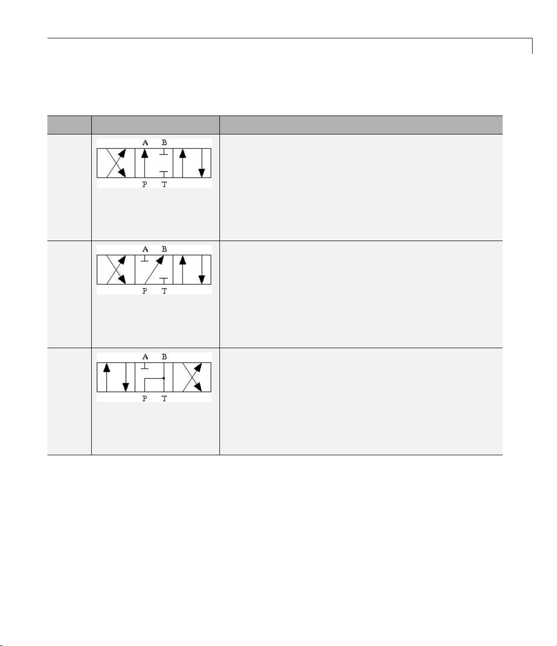
The other nine configurations are covered by the remaining 4-way directional valve blocks (A through K), as shown in the next table.

2-35

2 Modeling Hydraulic Systems

Other 4-Way Directional Valve Blocks

Block Name

4-Way Directional Valve A Contains two additional

4-Way Directional Valve B

4-Way Directional Valve C

4-Way Directional Valve D

4-Way Directional Valve E

Configuration

Description

normally-open, sequentially-located orifices. Valve displacement to the left or to the right closes the path to tank.

Ports P and A are permanently connected through fixed orifice. Orifices

P-B an d B-T are initially open

(underlapped).

Ports P and B are permanently connected through fixed orifice. Orifices

P-A, A-T and B-T are initially

open (underlapped).

Two orifices are installed in the P-A link. Port A never connects to port T.

Two orifices are installed in the P-B link. Port B never connects to port T.

4-Way Directional Valve F

2-36

Two parallel orifices in the P-A arm and two series orifices in the A-T arm.

Other 4-Way Directional Valve Blocks (Continued)

Modeling Directional Valves

Block Name

4-Way Directional Valve G Two parallel orifices in the

4-Way Directional Valve H

4-Way Directional Valve K

Configuration

Description

P-B arm and two series orifices in the B-T arm.

Two parallel orifices in the P-B arm and two series orifices in the P-T arm.

Two parallel orifices in the P-A arm and two series orifices in the P-T arm.

Building Blocks and How to Use Them

The Directional V alves library offers several pre built directional valve models. As indicated in their descriptions, all of them are symmetrical, continuous valves. In other words, the control member in 2-way, 3-way, 4-way, and 6-way valves can assume any position, controlled by the physical signal port S. The valves are symmetrical in that all the orifices the valve is built of are of the same type and size. The only possible difference between orifices is the orifice initial opening.

These configurations cover a substantial portion of real valves, but the directional valves family is so diverse as to make it practically impossible to have a library model for every member. Instead, Sim Hydraulics libraries offer a set of building blocks that is comprehensive enough to build a model for any real configuration. This section describes the rules of building a custom model of a directional valve.

All directional valve models are built of variable orifices. In SimHydraulics libraries, the following variable orifice models are available:

2-37

2 Modeling Hydraulic Systems

• Annular Orifice

• Orifice with Variable Area Round Holes

• Orifice with Variable Area Slot

• Variable Orifice

• Ball Valve

• Ball Valve with Conical Seat

• Needle Valve

• Poppet Valve

To simplify the way variable orifices are combined in a model, their instantaneous opening is computed in the same way for all types of orifices. The orifice opening is always computed in the direction the spool, or any other control member, opens the orifice. In other words, positive value of the opening co rresponds to open orifice, while negative value denotes overlapped, or closed, orifice. The origin always corresponds to zero-lap position, when the e dge of the control member coincides with the edge of the orifice. In the illustration below, origins are marked with area ro und holes (schematic on the left) and for the orifice with variable slot (schematic on the right). The opening is measured in both cases.

0 for the orifice with variable

x arrow denotes the direction in which orifice

2-38

Modeling Directional Valves

The instantaneous value of the orifice opening is determined as

hx x or

=+0i

where

Instantaneous orifice opening.

Initial opening. The initial opening value is positive for initially open (underlapped) orifices and negative for overlapped orifices.

Spool (or other control member) displacement from initial position, which controls the orifice.

Orifice orientation indicator. The variable assumes +1 value if a spool displacement in the globally assigned positive direction opens the orifice, and -1 if positive motion decreases the opening.

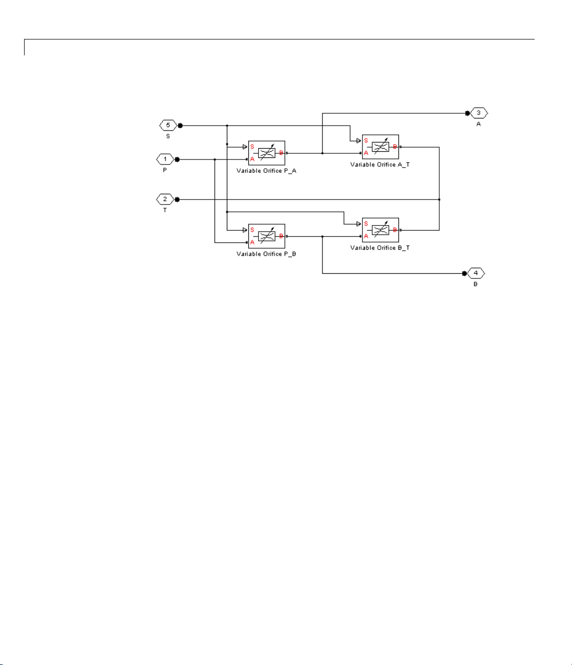
The number of variable orifices and the way they are connected are determined by the valve design. Usually, the model of a valve mimics the physical layout of a real valve. The illustration below shows an example of a 4-way valve, its symbol, an d an equ iv a len t circuit of its SimHydraulics model.

2-39

2 Modeling Hydraulic Systems

The 4-way valve in its simplest form is built of four variable orifices. In the equivalent circuit, they are named Orifice block, which is the most generic model of a variable orifice in the SimHydraulics libraries, is used in this particular example. You can use any other variable orifice blocks if the real valve design employs a configuration backed by a stock model, such as an orifice with round holes or rectangular slots, poppet, ball, or needle. In general, all orifices in the model can be simulated with different blocks or with the sam e block, but with different way of parameterization. For instance, two orifices can be represented by their pressure-flow characteristics, while two others can be simulated with the table-specified area variation option (for details, see the Variable Orifice block reference page).

P_A, P_B, A_T,andB_T. The Variable

2-40

The next example shows a no the r configuration of a 4-way directional valve. This valve unloads the pump in neutral position and requires six variable orifice blocks. The Orifice with Variable Area Round Holes blocks h ave been used as a variable orifice in this model. Port T1 corresponds to an intermediate point between ports P and T.

Modeling Directional Valves

Example of Building a Custom Directional Valve

Finally, let us consider a more complex directional valve example. The figure below shows basic elements of a front loader hydraulic system. Both the lift and the tilt cylinders are controlled by custom 3-position, 5-way valves, developed for this particular application. The valves are designed in such a

2-41

2 Modeling Hydraulic Systems

way that the pump delivery is diverted to tank (unloaded) if both cylinders are commanded to be in neutral position. The pump is disconnected from the tank if either of the two control valves is shifted from neutral position.

2-42

To develop a model, the physical version of the valve must be created first. The following illustration shows one of the possible configurations of the valve.

Modeling Directional Valves

The SimHyd configur

ation.

raulics model, shown below, is an exact copy of the physical valve

2-43

2 Modeling Hydraulic Systems

2-44

All the orifices in the model are closed (overlapped) in valve neutral position, except orifices extent that allows pump delivery to be discharged at low pressure.

P_T1_1 and P_T1_2. These two orifices should be set open to an

Modeling Low-Pressure Fluid Transportation Systems

In this section...

“How Fluid Transportation Systems Differ from Power and Control Systems” on page 2-45

“Available Blocks and How to Use Them ” on page 2-47

“Example of a Low-P ressure Fluid Transportation System” on page 2-49

How Fluid Transportation Systems Differ from Power and Control Systems

In hydraulics, the steady uniform flow in a component with one entrance and one exit is characterized by the following energy equation



VVgpp

−=



−

221

2 ρ

−

+−+

zzh

(2-1)

where

eperformedbyfluid

ow rate

velocity at the exit



, p

Work rat

Mass fl

Fluid

Fluid velocity at the entrance

Static pressure at the entrance and the exit, respectively

Gravity acceleration

Fluid density

, z

Elevation above a reference plane (datum) at the entrance and

the exit, respectively

ydraulic loss

Subscripts 1 and 2 refer to the entrance and exit, respectively. All the terms in Equation 2-1 have dimensions of height and are named kinematic head,

2-45

2 Modeling Hydraulic Systems

piezometric head, geometric head, and loss head, respectively. For a variety of reasons, analysis of hydraulic pow er and control systems is performed with respect to pressures, rather than to heads, and Equation 2-1 for a typical passive component is presented in the form

Vp gz Vp gzp

1211 2222

++ = ++ +

(2-2)

where

, p1,

, p2,

Term

ρgz

Velocity, static pressure, and elevation at the entrance, respectively

Velocity, static pressure, and elevation at the ex it, respectively

Pressure loss

is frequently referred to as kinematic, or dynamic, pressure, and

as piezometric pressure. Dynamic pressure terms are usually neglected

because they are very small, and Equation 2-2 takes the form

pgzp gzp

+=++ρρ

L1122

(2-3)

The size of a typical pow er and control system is usually small and rarely exceeds 1.5 – 2 m. To add to this, these systems operate at pressures in the

range 50 – 300 bar. Therefore,

ρgz

terms are negligibly small compared to static pressures. As a result, SimHydraulics components (with the exception of the ones designed specifically for low-pressure simulation, described in “Available B locks and How to Use Them ” on page 2-47) have been developed with respect to static pressures, with the following equations

2-46

pp fq

===()

qfpp

(, )

where

(2-4)

Modeling Low-Pressure Fluid Transportation Systems

Pressure difference between component ports

Flow rate through the component

Fluid transportation systems usually operate at low pressures (about 2 -4 bar), and the difference in component elevation with respect to reference plane can be very large. Therefore, geometrical head becomes an essential part of the energy balance and m ust be accounted for. In other words, the low-pressure fluid transportation systems must be simulated with respect to piezometric

ppgz

pressures

=+ρ

, rather than static pressures. This requirement is

reflected in the component equations

pp fqzz

===(, , )

qfppzz

(, ,,)

1212

(2-5)

Equations in the form Equation 2-5 must be applied to describe a hydraulic component with significant difference between port elevations. In hydraulic systems, there is only one type of such components: hydraulic pipes. The models of pipes intended to be used in low pressure systems must account for difference in elevation of their ports. The dimensions of the rest of the components are too small to contribute n oticeablytoenergybalance,andtheir models can be built with the constant ele vation assumption, like all the other SimHydraulics blocks. To sum it up:

• You can build models of low-pressure systems with difference in elev ations

of their components using regular SimHydraulics blocks, with the exception of the pipes. Use low-pressure pipes, described in “Available Blocks and HowtoUseThem”onpage2-47.

• When modeling low-pressure systems, you must use low-pressure pipe

blocks to connect all nodes with difference in elevation, because these are the only blocks that provide information about the vertical locations of the system parts. Nodes connected with any other blocks, such as valves, orifices,actuators,andsoon,willbetreatedasiftheyhavethesame elevation.

Available Blocks and How to Use Them

When modeling low-pressure hydraulic systems, use the pipe blocks from the Low-Pressure Blocks library instead of the regular pipe blocks. These blocks

2-47

2 Modeling Hydraulic Systems

account for the port elevation above reference plane and differ in the extent of idealization, just like their high-pressure counterparts:

• Resistive Pipe LP — Models hydraulic pip e with circular and noncircular

• Resistive Pipe LP with Variable Elevation — Models hydraulic pipe with

• Hydraulic Pipe LP — Models hydraulic pipe with circular and noncircular

• Hydraulic Pipe LP with Variable Elevation — Models hydraulic pipe with

cross sections and accounts for friction loss only, similar to the Resistive Tube block, available in the Simscape Foundation library.

circular and noncircular cross sections and accounts for friction losses and variable port elevations. Use this block for low-pressure system simulation in wh ich the pipe ends change their positions with respect to the reference plane.

cross sections and accounts for friction loss along the pipe length and for fluid compressibility, similar to the Hydraulic Pipeline block in the Pipelines library.

circular and noncircular cross sections and accounts for friction loss along the pipe length and for flui d compressibility, as well as variable port elevations. Use this block for low-pressure system simulation in which the pipe ends change their positions with respect to the reference plane.

2-48

• Segmented Pipe LP — Models circular hydraulic pipe and accounts

for friction loss, fluid compressibility, and fluid inertia, similar to the Segmented Pipe block in the Pipelines library.

Use these low-pressure pipe blocks to connect all hydraulic nodes in your model with difference in elevation, because these are the only blocks that provide informatio n about the vertical location of the ports. Nodes connected with any other blocks, such as valves, orifices, actuators, and so on, will b e treated as if they have the same elevation.

The additional models of pressurized tanks available for low-pressure system simulation include:

• Constant Head Tank — Represents a pressurized hydraulic reservoir,

in which fluid is stored under a specified pressure. The size of the tank is assumed to be large enough to neglect the pressurization and fluid level change due to fluid volume. The block accounts for the fluid level elevation with respect to the tank bottom, as well as for pressure loss in

Modeling Low-Pressure Fluid Transportation Systems

the connecting pipe that can be caused by a filter, fittings, or some other local resistance. The loss is specified with the pressure loss coefficient. Theblockcomputesthevolumeoffluidinthetankandexportsitoutside through the physical signal port V.

• Variable Head Tank — Represents a pressurized hydra ulic reservoir,

in which fluid is stored under a specified pressure. The pressurization remains constant regardless of volume change. The block accounts for the fluid lev el change caused by the volume variation, a s well as for pressure loss in the connecting pipe that can be caused by a filter, fittings, or some other local resistance. The loss is specifie d with the pressure loss coefficient. The block computes the volume of fluid in the tank and exports it outside through the physical signal port V.

• Variable Head Two-Arm Tank — Represents a two-arm pressurized tank,

in which fluid is stored under a specified pressure. The pressurization remains constant regardless of volume change. The block accounts for the fluid lev el change caused by the volume variation, a s well as for pressure loss in the connecting pipes that can be caused by a filter, fittings, or some other local re sis tance. The loss is specified with the pressure loss coefficient at each outlet. The block computes the volume of fluid in the tank and exports it outside through the physical signal port V.

• Variable Head Three-Arm Tank — Represents a three-arm pressurized

tank, in which fluid is stored under a specified pressure. The pressurization remains constant regardless of volume change. The block accounts for the fluid lev el change caused by the volume variation, a s well as for pressure loss in the connecting pipes that can be caused by a filter, fittings, or some other local re sis tance. The loss is specified with the pressure loss coefficient at each outlet. The block computes the volume of fluid in the tank and exports it outside through the physical signal port V.

Example of a Low-Pressure Fluid Transportation System

The following illustration shows a simple system consisting of three tanks whose bottom surfaces are located at heights H1, H2, and H3, respectively, from the reference plane. The tanks are connected by pipes to a hydraulic manifold, which may contain any hydraulic elements, such as valves, orifices, pumps, accumulators, other pipes, and so on, but these elements have one feature in common – their elevations are all the same and equal to H4.

2-49

2 Modeling Hydraulic Systems

2-50

The models of tanks account for the fluid level heights F1, F2, and F3, respectively, and represent pressure at their bottoms as

pgF i

==ρ for 1 2 3,,

The components inside the manifold can be simulated with regular SimHydraulics blocks, like you would use for hydraulic power and control systems simulation. The pipes must be simulates with one of the low-pressure pipe models: Resistive Pipe LP, Hydraulic Pipe LP, or Segmented Pipe LP, depending on the required extent of idealization. Use the Constant Head Tank or Variable Head Tank blocks to simulate the tanks. For details of implementation, see the Water Supply System ( and the Fluid Transportation System with Three Tanks ( demos.

sh_water_supply_system)

sh_three_tanks)

Examples

Use this list to find examples in the documentation.

A Examples

Getting Started

“Creating a Simp

le Model” on page 2-8

Modeling Directional Valves

“Example of Building a Custom Directional Valve” on page 2-41

Modeling Lo

w-Pressure Fluid Transportation Systems

“Example of a Low-Pressure Fluid Transportation System” on page 2-49

A-2

Index

IndexH

hydraulic fluids

specifying properties 2-6

SimHydraulics® software

about 1-2 block library structure 2-2 simulating models 1-7

Index-1

Mathworks SIMHYDRAULICS 1 user guide

Specifications and Main Features

Frequently Asked Questions

User Manual

Getting Started

Product Overview

Product Description

Assumptions and Limitations

ThePhysicalModelingProductFamily

Getting Online Help

Using the MATLAB Help System for Documentation and Demos

The MathWorks Online

Related Products

Product Requirements

Other Related Products

Modeling Physical Networks with SimHydraulics Blocks

Running Hydraulic Models

Troubleshooting Hydraulic Models

Using Simscape Editing Modes

Modeling Hydraulic Systems

Introducing the SimHydraulics Block Libraries

Library Structure Overview

Using the Simulink Library Browser to Access the Block Libraries

Essential Steps to Building a Hydraulic Model

Overview of Modeling Rules

Working with Fluids

Creating a Simple Model

Building a SimHydraulics Diagram

Modifying Initial Settings

Running the Simulation

Adjusting the Parameters

Changing the Valve Input Signal

Changing the Cylinder Load Parameters

Changing the Rod Position Output Units

Modeling Power Units

Modeling Directional Valves

TypesofDirectionalValves

4-Way Directional Valve Configurations

Basic 4-Way Directional Valve Configurations

Other 4-Way Directional Valve Blocks

Building Blocks and How to Use Them

Example of Building a Custom Directional Valve

Modeling Low-Pressure Fluid Transportation Systems

Available Blocks and How to Use Them

Example of a Low-Pressure Fluid Transportation System

Examples

Getting Started

Modeling Directional Valves

Index