Mathworks SIMDRIVELINE 1 user guide

Download

SimDriveline™ 1

User’s Guide

How to Contact The MathWorks

www.mathworks. comp.soft-sys.matlab Newsgroup www.mathworks.com/contact_TS.html Technical Support

suggest@mathworks.com Product enhancement suggestions

bugs@mathwo doc@mathworks.com Documentation error reports service@mathworks.com Order status, license renewals, passcodes

info@mathwo

com

rks.com

Web

Bug reports

Sales, prici

ng, and general information

508-647-7000 (Phone)

508-647-7001 (Fax)

The MathWorks, Inc. 3 Apple Hill Drive Natick, MA 01760-2098

For contact information about worldwide offices, see the MathWorks Web site.

SimDriveline™ User’s Guide

The software described in this document is furnished under a license agreement. The software may be used or copied only under the terms of the license agreement. No part of this manual may be photocopied or reproduced in any form without prior written consent from The MathW orks, Inc.

FEDERAL ACQUISITION: This provision applies to all acquisitions of the Program and Documentation by, for, or through the federal government of the United States. By accepting delivery of the Program or Documentation, the government hereby agrees that this software or documentation qualifies as commercial computer software or commercial computer software documentation as such terms are used or defined in FAR 12.212, DFARS Part 227.72, and DFARS 252.227-7014. Accordingly, the terms and conditions of this Agreement and only those rights specified in this Agreement, shall pertain to and govern theuse,modification,reproduction,release,performance,display,anddisclosureoftheProgramand Documentation by the federal government (or other entity acquiring for or through the federal government) and shall supersede any conflicting contractual terms or conditions. If this License fails to meet the government’s needs or is inconsistent in any respect with federal procurement law, the government agrees to return the Program and Docu mentation, unused, to The MathWorks, Inc.

Trademarks

MATLAB and Simulink are registered trademarks of The MathWorks, Inc. See

www.mathworks.com/trademarks for a list of additional trademarks. Other product or brand

names may be trademarks or registered trademarks of their respective holders.

Patents

The MathWorks products are protected by one or more U.S. patents. Please see

www.mathworks.com/patents for more information.

Revision History

August 2004 Online only New for Version 1.0 (Release 14+) October 2004 Online only Revised for Version 1.0.1 (Release 14SP1) March 2005 Online only Revised for Version 1.0.2 (Release 14SP2) April 2005 Online only Revised for Version 1.1 (Release 14SP2+) September 2005 O nline only Revised for Version 1.1.1 (Release 14SP3) March 2006 First printing Revised for Version 1.2 (Release 2006a) September 2006 O nline only Revised for Version 1.2.1 (Release 2006b) March 2007 Online only Revised for Version 1.3 (Release 2007a) September 2007 O nline only Revised for Version 1.4 (Release 2007b) March 2008 Online only Revised for Version 1.5 (Release 2008a) October 2008 Online only Revised for Version 1.5.1 (Release 2008b) March 2009 Online only Revised for Version 1.5.2 (Release 2009a) September 2009 O nline only Revised for Version 1.5.3 (Release 2009b) March 2010 Online only Revised for Version 1.5.4 (Release 2010a)

Introducing SimDriveline Software

Product Overview ................................. 1-2

Product Definition Driveline Simulation and Physical Modeling

................................. 1-2

........... 1-2

Contents

Introducing SimDriveline Software

With SimDriveline™ software, you can model drivetrain and powertrain systemsinaneasy,naturalwaywithinMATLAB chapter introduces you to SimDriveline software, with an overview and an example of modeling drivetrains.

• “Product Overview” on page 1-2

• “Related Products” on page 1-4

• “Running a Demo Model” on page 1-6

• “What Can You Do with Sim Driveline Software?” on page 1-20

• “Learning More” on page 1-25

and Simulink®.This

1 Introduc ing SimDriveline™ Software

Product Overview

In this section...

“Product Definition” on page 1-2

“Driveline Simulation and Physical Modeling” on page 1-2

Product Definition

SimDriveline software is a block diagram modeling environment for the engineering design and simulation of drivelines, or idealized powertrain systems. A driveline propels a vehicle or craft by transferring its engine torque and rotational power into vehicle kinetic energy and translational momentum. The vehicle moves through or on a medium (air, water, ground) which propels it by reaction forces an d which acts as a load on th e engine. Drivelines consist of b odies spinning around fixed axes and subject to Newton’s laws of motion. T he bodies can revolve about one axis, multiple parallel axes, or multiple nonparallel axes. Simp l e and complex gears constrain the bodies to revolve together and transfer torque up and down the driveline axes. Locking and unlocking clutches switch the driveline from one gear set to another. Gears and clutches make up transmissions.

1-2

With SimDriveline software, you represent a driveline with a connected block diagram, like other Simulink models, and you can group blocks in to hierarchical subsystems. You can initiate and maintain rotational motion in a driveline with actuators wh ile measuring, via sensors, the motions of driveline elements and the torques acting on them. You can return sensor signals to the driveline via actuators, forming feedback loops and the basis for controls.

The SimDriveline libraries offer blocks to represent rotating bodies; gear constraints among bodies; dynamic elements such as spring-damper forces, rotational stops, and clutches; transmissions; and sensors and actuators. You can also analyze linearized versions of your SimDriveline models and generate code from them.

Driveline Simulation and Physical Modeling

SimDriveline software is based on the Simscape™ environment, the platform product for the Simulink Physical Modeling family, encompassing the

Product Overview

modeling and design of systems according to basic physical principles. Simscape software runs within the Simulink environment and interfaces seamlessly with the rest of Simulink and with MATLAB. Unlike other Simulink blocks, which represent mathematical operations or operate on signals, Simscape blocks represent physical components or relationships directly.

Note This SimDriveline User’s Guide assumes that you have some experience with modeling drivetrains and with building and running models in Simulink.

1-3

1 Introduc ing SimDriveline™ Software

Related Products

In this section...

“Required Products” on page 1-4

“Other Related Products” on page 1-4

Required Products

You must have current versions of the following products installed to use the SimDriveline product:

• MATLAB

• Simulink

• Simscape

Other Related Products

The related products listed on the SimDriveline product page at the MathWorks™ Web site include toolboxes and blocksets that extend the capabilities of MATLAB and Simulink. These products will enhance your SimDriveline experience in various applications.

1-4

Physical Modeling Product Family

Use the Physical Modeling product family to model physical systems in Simulink. In addition to SimDriveline software, they include:

• Simscape, the platform and unifying environment for Physical Modeling

products

• SimElectronics

• SimHydraulics

• SimMechanics™, for modeling and simulating mechanical systems

• SimPowerSystems™, for modeling and simulating electrical power systems

, for modeling and simu l ati ng el ectronic systems

, for modeling and simulating hydromechanical systems

For Information About MathWorks Products

For more information about any MathWorks software products, see either

• The online documentation for that product if it is installed

• The MathWorks Web site at

www.mathworks.com; see the “Products” section

1-5

1 Introduc ing SimDriveline™ Software

Running a Demo Model

In this section...

“What the Model Represents” on page 1-6

“What the Model Illustrates” o n page 1-6

“Opening the M odel” on page 1-7

“Running the Model” on page 1-11

“Modifying the Model” on page 1-15

What the Model Represents

The demo model of this section, drive_crcr_ideal, simulates a complete drivetrain. This model will help you understand how to model driveline components with SimDriveline blocks, connect them into a realistic model, use Simulink blocks as well, and simulate and modify a drivetrain model.

1-6

The d riveline mechanism modeled here is part of a full vehicle, without the engine or engine-drivetrain coupling, and without the final differential and wheel assembly. The model includes an actuating torque, driver and driven shafts, a four-speed transmission, and a braking clutch.

What the Model Illustrates

The drive_crcr_ideal model contains a driveline that accepts a driving torque and transfers this torque and the associated angular motion from the input or drive shaft to an output or driven shaft through a transmission. The model includes a CR-CR (carrier-ring–carrier-ring) four-speed transmission subsystem, based on two gears and four clutches. (The demo does not use the reverse gear available in the CR-CR transmission.) You can set the transmission to four different gear combinations, allowing four different effective torque and angular velocity ratios. A fifth clutch, outside the transmission, acts as a brake on the driven shaft.

The CR-CR 4-Speed Transmission subsystem illustrates a critical feature of transmission design, the clutch schedule. Tobefullyengaged,the transmission, with four clutches and two gears, requires two clutches to be locked and the other two unlocked at any time. (The transmission’s

Running a Demo Model

reverse clutch is not counted here.) The choice of which two clutches to lock determines the effective gear ratio across the transmission. T he clutch schedule is the table of locked and free clutches corresponding to different gear settings. If all four clutches are unlocked, the transmission is in neutral. If the clutches are completely disengaged, no torque or angular motion at all is transferred across the transmission.

Clutch Schedule for the CR-CR 4-Speed Transmission

Gear Setting

Clutch A State

Clutch B State

Clutch C State

Clutch D State

L FFL

L F L F

LLFF

F LLF

L = locked, F = free

Opening the Model

To get started q u ickly with the CR-CR transmission demo model, follow either of these steps:

• Enter

• If you are working with the MATLAB Help browser, click the model name

Opening General SimDriveline Demos

You can open the complete SimDriveline demos list by:

drive_crcr_ideal at the MATLAB command line.

drive_crcr_ideal here.

1 Clicking the Start button on the lower left of the MATLAB desktop.

2 In the pop-up menu, selecting Simulink,thenSimDriveline,andthen

Demos.

This opens the SimDriveline demos list in the MATLAB Help browser.

1-7

1 Introduc ing SimDriveline™ Software

You can locate and select any specific demo entry from the list of models.

Alternatively, you can open the same SimDriveline demos list by entering

demo simulink simdriveline or demo('simulink','simdriveline') at

the MATLAB command line.

The Block Diagram Model

Examine the model and its structure. The main model window contains the CR-CR transmission subsystem, the input or driver shaft assembly, and the output or drive n shaft assembly. Each assembly consists of a wheel with applied kinetic friction. The driver shaft transmits an externally specified torque down the driveline.

The m ain model also includes a brake clutch. When this clutch is locked, the driven shaft stops turning. This clutch must remain unlocked if the C R-C R transmission is engaged.

1-8

nModelWindow

Mai

Running a Demo Model

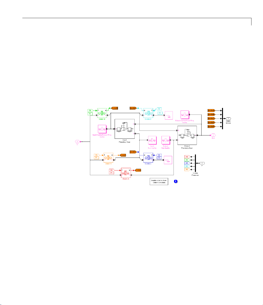
What the Model Contains — Opening the Subsystems

Open each subsystem in turn.

• The CR-CR 4-Speed Transmission subsystem is a set of fou r clutches,

two planetary gears, and four inertias (rotating bodies). (Ignore the

reverse gear and associated clutch.) Within the subsystem, open the

clutch schedule block to see the four possible (forward) gear settings for

the C R-CR 4-speed transmission. Exactly two clutches must be locked at

any one time for the transmission to be engaged and to avoid conflicting

constraints on the gear motions.

CR-CR 4-Speed Transmission Subsystem

1-9

1 Introduc ing SimDriveline™ Software

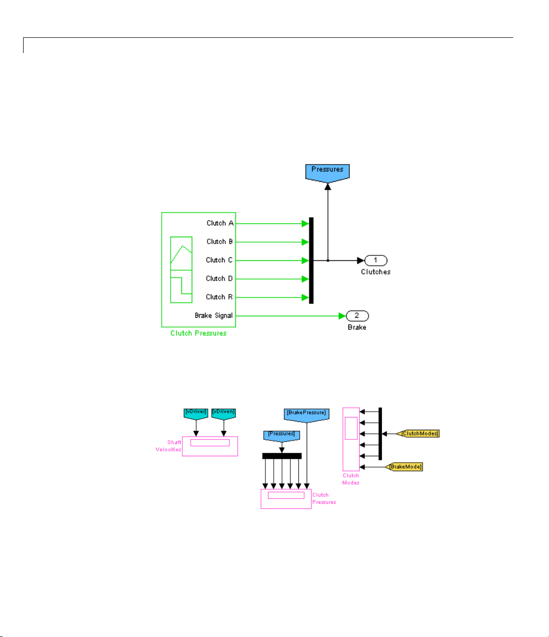
• The Clutch Control subsystem provides the pressures that lock the

necessary clutches. The clutch controller is programmed to move the

transmission through a fixed sequence of gears, then unlock all the

transmission clutches, allowing the driven shaft to “coast” for a time, and

then engage and lock the brake clutch to stop the driven shaft.

1-10

Clutch Control Subsystem

• The Scopes subsystem provides Scope blocks to display the clutch pressure,

driver and driven shaft velocity, and clutch mode signals.

Scopes Subsystem

Running a Demo Model

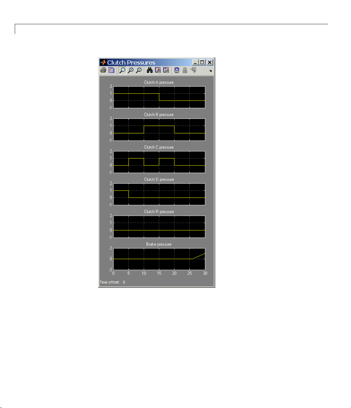
Running the Mode

To display the CR

1 Open the Scopes

Scopes subsyst

2 Click Start. The model steps through the gears and then brakes.

3 Observe how the clutch pressure signals move the transmission into

one gear after another, at 0, 5, 10, and 15 seconds of simulation time.

Compare these clutch pressure signals to the clutch schedule in the CR-CR

transmission subsystem to determine which gear settings the model is

implementing. (In fact, the model ste ps through gears 1, 2, 3, and 4, before

coasting and then braking.)

-CR driveline mo del’s behavior,

subsystem and then each of the Scope blocks. Close the

em.

1-11

1 Introduc ing SimDriveline™ Software

1-12

Running a Demo Model

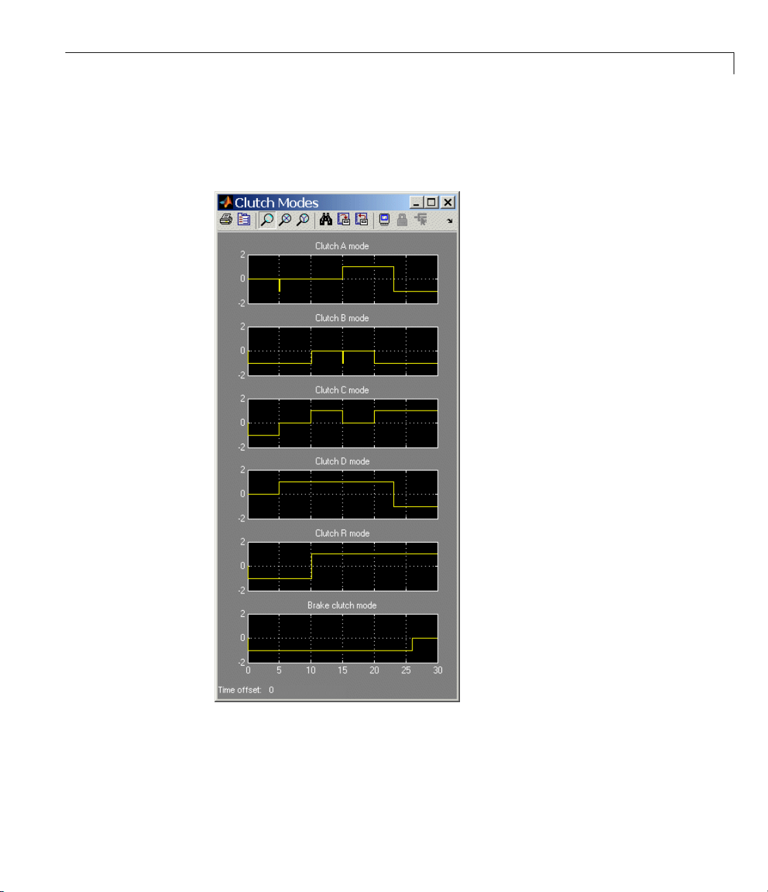
4 Observe the clutch modes at the same time. When a clutch mode is zero,

that clutch is locked. The sequence of clutch locking and unlocking matches

the sequence from the clutch schedule.

1-13

1 Introduc ing SimDriveline™ Software

5 Compare the angular velocities of the driven and driver shafts. The effect

of the transmission is the result of the two planetary gears coupled in

different ways in the different gear settings. The effective drive ratio

of output to input shafts is the reciprocal of the ratio of output to input

angular velocities.

1-14

6 Observe what happens at 20 seconds. The transmission clutch pressures

drop to zero, and the transmission disengages. The transmission ceases

to transfer angular m otion and torque from the driver to the driven shaft,

and the driven shaft continues to spin simply from inertia. A small kinetic

friction damping gradually slows the driven shaft over the next 6 seconds.

Running a Demo Model

7 At 26 seconds of simulation time, the brake clutch pressure begins to rise

from zero, and the brake clutch engages. The driven shaft decelerates more

drastically now. Between 26.0 and 26.1 seconds, the brake clutch locks,

and the driven shaft stops rotating completely.

Modifying the Model

You can modify this demo model to explore other SimDriveline features. Here you modify and rerun the model to investigate two aspects of its motion.

• Measure the effective drive ratio of the CR-CR transmission in each gear

setting that it steps through.

• Change the gear sequence.

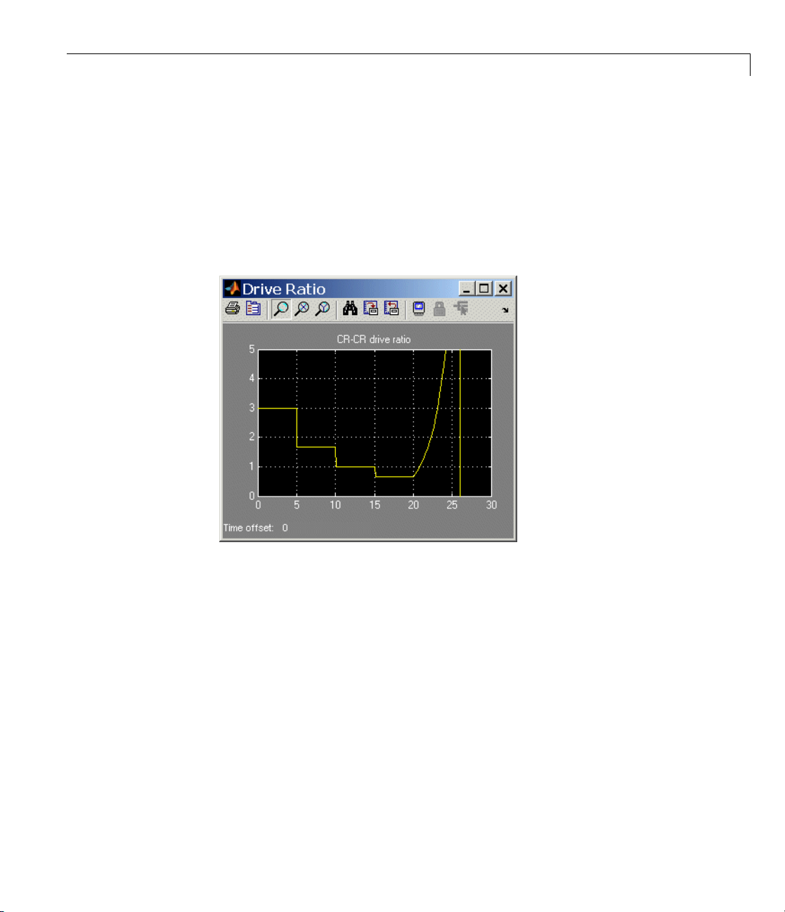
Measuring the Drive Ratio of the CR-CR Transmission States

The gear ratio (output to input) is the ratio of the output gear wheel radius to the input gear radius. Equivalently, thegearratioistheratioofthenumber of teeth on the output gear wheel to the number on the input wheel, or the ratio of the output torque to the input torque. The ratio of the angular velocities of output to input is the reciprocal of this gear ratio.

A transmission is a set of coupled gears. But for a particular transmission gear setting, the ratio of driven (output) shaft velocity to the driver (input) is fixed. Its reciprocal, the drive ratio, is like a gear ratio of an individ ual gear coupling, but for the whole transmission.

1-15

1 Introduc ing SimDriveline™ Software

Add and connect the Simulink blocks necessary to measure the drive ratio of the transmission.

1 From the Simulink Math Op e ra tions lib rary, copy a Divide block and, from

the Simulink Sinks library, copy a Scope block.

2 From the Torque Driver subsystem outport, branch a signal line from

Motion Sensor1’s angular velocity output and connect it to the

on the Divid e block. From the velocity output of Motion Sensor2, on the

driven (output) shaft, again branch a signal line. Connect it to the ÷ inport

on the Divide block.

The effective output-to-input drive ratio is the ratio of input to output

velocities.

3 Connect the outport of the Divide block to the Scope. Rename Scope to

Drive Ratio.

X inport

1-16

CR-CR 4-Speed Model with Drive Ratio Measurement

Running a Demo Model

4 OpentheDriveRatioscopeandrestartthedemo. Observehowthedrive

ratio steps through a sequence of five-second states, in parallel with the

clutch pressures and clutch modes, until it reaches 20 seconds. The

drive ratio measurement after 20 seconds is not meaningful because the

transmission is uncoupled.

Just after 26 seconds, the driven shaft velocity drops to zero, and the Div ide

block produces divide-by-zero warnings at the MATLAB command line.

5 Look inside the CR-CR 4-Speed Trans mission subsystem for the Clutch

Schedule block and open it. Consult the drive ratios for each gear, 1, 2,

3, and 4, in terms of the gear ratios of the transmission’s two Planetary

Gears. Determine the numerical values for these drive ratios for gear

settings1,2,3,and4andcheckthemagainstthevaluesdisplayedinthe

Drive Ratio scope.

The drive ratio sequence should be 3, 5/3, 1, and 2/3, respectively, for the

first, second, third, and fourth intervals of five seconds each.

nging the Transmission Gear Sequence

Cha

The d rive_crcr_ideal demo, when you open it, is programmed to step through CR-CR gear settings 1, 2, 3, and 4, before disengaging. Modify it to step through settings 1, 2, 3, and 1, then disengage. T he fourth gear requires

1-17

1 Introduc ing SimDriveline™ Software

A, B, C, and D to be free, locked, locked, and free, respectively . You will modify the clutch pressure signal sequence from 15 to 20 seconds so that the transmission is set in first, not fourth, gear. The first gear requires clutches A, B, C, and D to be locked, free, free, and locked, respectively.

1 Open the C lutch Control and CR-CR transmission subsystems. Within

the transmission, open the Clutch Schedule block and review the clutch

lockings for each gear setting.

2 Open the Signal Builder block, labeled Clutch Pressures, to view the clutch

pressure signals.

Modify clutch pressure signals A, B, C, and D so that, between 15 and 20

seconds, clutches A and D are locked (not free) and clutches B and C are

free (not locked). Sufficient pressure will lock the clutches, while zero input

pressure leaves a clutch unlocked.

1-18

Modified CR-CR 4-Speed Transmission Clutch Pressures

Running a Demo Model

3 Restart the model. Observe that between 15 and 20 seconds of simulation

time the clutch pressures, the clutch modes, and the driven shaft velocity

are now different from the original version of the model.

Check the effective drive ratio between 15 and 20 seconds to confirm that

the CR-CR transmission during that time is set in gear 1, not gear 4. This

fourth interval of five seconds should exhibit a drive ratio of 3 instead of 2/3.

1-19

1 Introduc ing SimDriveline™ Software

What Can You Do with SimDriveline Software?

In this section...

“About SimDriveline Software” on page 1-20

“Modeling Drivetrains” on page 1-20

“Connector Ports and Connection Lines” on page 1-21

“Inertias and Gears” on page 1-22

“Complex Driveline Elements” on page 1-22

“Actuating and Sensing Motion” on page 1-23

“Simulating and Analyzing Motion” on page 1-24

About SimDriveline Software

SimDriveline software is a set of block libraries and special simulation features for use in the Simulink environment. You connect SimDriveline blocks to normal Simulink blocks through Sensor and Actuator blocks.

1-20

The blocks in these libraries are the e lem ents you need to model driveline systems consisting of any number of rotating inertias, rotating about one or more axes, constrained to rotate together by gears, which transfer torque to different parts of the driveline. You can represent drivelines with components organized into hierarchical subsystems, as in normal Simulink models. You can add complex dynamic elements such as clutches and transmissions, actuate bodies with external torques or motions, integrate the Newtonian rotational dynamics, and measure the resulting motions.

Modeling Drivetrains

SimDriveline software extends Simulink with blocks to specify a driveline’s components and properties and to solve the equations of motion. The blocks are similar to other Simulink blocksets, with some properties unique to SimDriveline software.

These are the major steps you follow to build and run a SimDriveline model representation of a driveline:

What Can You Do with SimDriveline™ Software?

1 Specify rotational inertia for each body and connect the bodies with

driveline connection lines representing driveline axes. If needed, ground

the driveline to one or more housings fixed in space.

2 Constrain the driveline axes to rotate together by connecting them with

gears. Gears impose static constraints on driveline motions and transfer

torques at fixed ratios.

3 As necessary and desired, add dynamic driveline elements that transfer

torque and motion among driveline axes in a nonstatic way. These

elements include internal torque-generating components such as damped

springs, clutches and transmissions, and torque converters. You can also

construct and connect your own dynamic elements.

4 Setupactuatorsandsensorstoinitiateandrecordbodymotions,aswellas

apply external torques to the driveline.

5 Connect the Sim Driveline motion solv er to the driveline and configure it.

Start the simulation, calling the Simulink solvers to find the motions of the

system. Display and analyze the motion.

Connector Ports and Connection Lines

Most SimDriveline blocks have special driveline ports . You connect driveline ports with driveline connection lines, distinct from normal Simulink lines. Driveline connection lines represent physical rotation axes along which torque is transferred and around which inertias rotate.

• You can connect driveline ports only to other driveline ports.

• The driveline connection lines that connect driveline ports together are

not normal Simulink lines, which carry signals or indicate mathematical

operations. You cannot connect driveline lines directly to Simulink inports

and outports >.

• Two directly connected driveline components must corotate at the same

angular velocity.

• You can branch SimDriveline connection lines. When you do so, components

directly connected with one another continue to share the same angular

velocity. The torque transferred along the driveline axis is divided among

the multiple components connected by the branches. How the torque is

divided is determined by the driveline dynamics.

1-21

1 Introduc ing SimDriveline™ Software

The sum of all torques flowing into a branch point equals the sum of all

torques flowing out.

Inertias and Gears

SimDriveline software defines a drive line as a collection of bodies rotating about driveline axes represented by connection lines. The bodies are defined by their rotational inertias. The lines carry the rotational degrees of freedom (DoF) and, unconstrained, rotate freely. Directly connecting one body to another constrains both bodies to rotate at th e same angular velocity. A torque applied to one body is effectively applied to both.

You can also ground driveline axes to housings that do not move and that represent infinite effective inertia.

Note All SimDriveline rotational DoFs are ab sol ute and m easured with respect to a single implicit global coordinate system at rest.

1-22

In a real driveline, the bodies can also be connected indirectly by gears that couple driveline axes. The gears constrain the axes to rotate together. T hese gears can be simple or complex and can couple two or more axes. The g ears have two roles:

• They constrain the connected axes to corotate at angular velocities in

fixed ratio or ratios.

• They transfer the torques flowing along one or more axes to other axes,

also in fixed ratio or ratios.

Complex Driveline Elements

Tip These blocks serve as suggestions for developing variant or entirely new

models to simulate the same components. You can study these subsystems by looking under their masks. If necessary, break the block’s library link before modifying it, and then create your own version. Or create your own completely new block from scratch.

What Can You Do with SimDriveline™ Software?

Tocreatemorerealisticdrivelinemodels, you elaborate on simple drivelines consisting of inertias and gears by adding complex mechanical elements that generate torques internally within the driveline, between one axis and another. Certain SimDriveline blocks encapsulate as subsystems entire models of complex dri veline elements:

• Clutches that model the locking and unlocking of pairs of driveline axes by

applying kinetic and static friction.

Note In the default case, adding clutches introduces algebraic loops (mode

iterations), non-time-based simulation steps.

• Transmission models that incorporate multigear sets and clutches into a

single subsystem

• Vehicle component models that represent engines, tires, and vehicle

dynamics

• Specialized torque models, such as torque converters, bilateral stops, and

damped spring-like torsion

Actuating and Sensing Motion

Sensors and Actuators are the blocks you use to interface between SimDriveline blocks and normal Simulink blocks:

• Actuator blocks impart motion to driveline axes, e ither at zero time or

through the course of a simulation, and impose externally defined torques

on the bodies of a driveline.

• Sensor blocks measure the motions of, and the torques transferred along,

theaxesofadrivelinesystem.

Actuating inputs and sensor outputs are Simulink signals that you can define and use like any other Simulink signal. For example, you can connect a Sensor output to a Simulink Scope block and display the torques in a driveline as functions of time.

1-23

1 Introduc ing SimDriveline™ Software

Simulating and A

Once you specify the bodies with g of finding the s prepare it for s environment. Newtonian dyn torques and co

Once your mod motions and i

all the rotational inertias of the bodies and interconnect

ears and other driveline elements, the dynamical problem

ystem’s motion is solvable. To finish a driveline model and

imulation, you must connect the driveline to the SimDriveline

The environment defines the solver that integrates the

amics for the system, applying all internal and external

nstraints to find the motions of the bodies.

el is ready for simulation, you can run it and analyze its

nternal torques.

nalyzing Motion

Trimming and Linearizing the Motion

In many cas of motions torques, y trajector consists

Aspecial searchi acceler tools in how the system

es, you do not know the torques necessary to produce a given set

. By motion-actuating your driveline and measuring the resulting

ou can find the torques necessary to produce a specified motion y. This technique inverts the canonical approach to dynamics, which of finding motions from torques.

case of inverse dynamics is trimming. This technique involves

ng for steady-state motions of the bodies, when their angular

ations and the torques they experience vanish. Using the linearization

Simulink, you can perturb such a steady motion state slightly to find

system responds to small disturbances. Theresponseindicatesthe

’s stability and suitability for controllers.

1-24

Generating Code — Clutches and Algebraic Loops

SimDr Realvers enha

The p and The gen

iveline software is compatible with Simulink Acceleration modes,

Time Workshop

ions of the models you create originally in Simulink with block diagrams,

ncing simulation speed and model portability.

resence of clutches in a driveline model induces mode iterations

dynamical discontinuities and triggers algebraic loops in Simulink.

se discontinuities and algebraic loops place certain restrictions on code

eration.

and xPC Target™ software. They let you generate code

Learning More

In this section...

“Using the MATLAB Help System for Documentation and Demos” on page 1-25

“Finding Special SimDriveline Help” on page 1-25

Using the MATLAB Help System for Documentation and Demos

Youcangethelponlineinanumberofwaystoassistyouwhileyouuse SimDriveline software. The MATLAB help browser allows you to access the documentation and demo models for a ll the MATLAB and Simulink based products that you have installed. The online help includes an online index and search system.

Consult the MATLAB Getting Started Guide for more about the MATLAB help system.

Learning More

Finding Special SimDriveline Help

This user’s guide includes these reference chapters:

• Appendix A, “Technical Conventions” explains special conventions,

abbreviations, and units.

• Appendix B, “Bibliography” lists external references on driveline and

powertrain modeling and related topics.

In addition, many SimDriveline demos have help links represented by the information symbol

in the Help browser.

. Click this symbol to open that demo’s documentation

1-25

1 Introduc ing SimDriveline™ Software

1-26

Simple Models

This chapter introduces you to modeling drivetrains in the SimDriveline environment. After showing you how you how to access the SimDriveline block library and reviewing the essential rules of connecting blocks and transferring angular motion and torque, it moves you from modeling simple gears to simulating a full car in a series of short tutorials.

• “Introducing the SimDriveline Block Libraries” on page 2-2

• “Essential Steps to Building a Driveline Model” on page 2-7

• “Representing and Transferring Driveline Motion and Torque” on page 2-9

• “Actuating Drivelines with Torques and Motions” on page 2-22

• “Controlling Gear Couplings with Clutches” on page 2-28

• “Combining Clutches and Gears into Transmissions” on page 2-42

• “Modeling and Simulating a Complete Car” on pag e 2-58

This user’s guide assumes that you are familiar with building models in Simulink. If not, see the Simulink documentation.

2 Simple Models

Introducing the SimDriveline Block Libraries

In this section...

“About the SimDriveline Block Library” on page 2-2

“Accessing the Libraries” on page 2-2

“Using the Libraries ” on page 2-4

About the SimDriveline Block Library

SimDriveline software is organized into a set of libraries of closely related blocks. This section shows you how to opentheseSimDriveline block libraries and explains the nature of each library.

Accessing the Libraries

There are several ways to open the SimDriveline block library.

2-2

You can access the blocks through the Simulink Library Browser. Open the

browser by clicking the Simulink button then the SimDriveline subentry, in the contents tree.

. Expand the Simscape entry,

Introducing the SimDriveline™ Block Libraries

You can also access the blocks directly inside the SimDriveline library in several ways:

• In the Simulink Library Browser, right-click the SimDriveline subentry

under Simscape and select Open SimDriveline Library. The library appears.

• Click the Start button in the lower-left corner of your MATLAB desktop.

In the pop-up menu, select Simulink,thenSimDriveline,thenBlock Library.

• Enter

drivelib at the MATLAB command line.

2-3

2 Simple Models

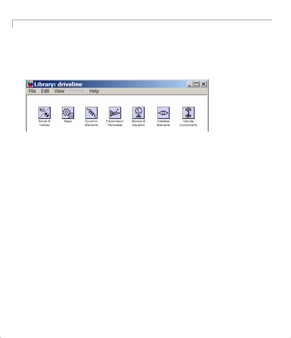
SimDriveline Library

Once you perform one of these steps, the SimDriveline library opens. This library displays seven top-level block groups. You can expand each library by double-clicking its icon.

The next section summarizes the blocks of each library and their use. For explanations of individual blocks, consult the SimDriveline “Block Reference” reference.

2-4

Using the Libraries

The SimDriveline block library is organized into separate libraries, each with a different type of driveline block.

Solver & Inertias

The Solvers & Inertias library provides the Inertia block, which represents a rotating body specified by its moment of inertia, the fundamental unit of driveline modeling. It also contains the Housing block, which represents an immobile rotational ground.

Finally, the library contains the Driveline Environment block, which configures the driveline settings of a SimDriveline block diagram, and the Shared Environment block, which allows you to connect two driveline block diagrams in a nonphysical way so that they share the same driveline environment settings.

Gears

The Gears library contains blocks that represent simple and complex gears, driveline elements that couple distinct driveline axes and constrain their

Introducing the SimDriveline™ Block Libraries

relative motions. The Gear blocks range from simple two-wheel gear couplings with fixed and variable gear ratios, to complex multiwheel and multiaxis gears such as planetary and differential gears.

Dynamic Elements

The Dynamic Elements library contains blocks that model such critical drivetrain components as clutches, torque converters, damped springs, and stops. Dynamic elements generate internal driveline torques.

The blocks of this library serve as suggestions for developing variant or entirely new models to simulate the same components. Look under the block mask, break the block’s library link before modifying it, and create your own version.

Transmission Templates

The Transmission Templates are a set of predesigned transmission examples constructed from gears, clutches, and inertias. You can copy and use these examples in your drivetrain models.

Transmission templates copied into your model are not linked to the block library. You can modify and rebuild these template copies at will.

Sensors & Actuators

The Sensors & Actuators library provides blocks for sensing and initiating the motions of driveline axes and applying and sensing torques along those axes.

Interface Elements

The Interface Elements library enables connections between SimDriveline driveshaft connection lines and Simscape mechanical rotational motion.

Vehicle Components

The Vehicle Components library contains blocks that represent components of a full vehicle beyond the drivetrain itself. It includes models of engines, wheeled vehicles, and tires in contact with the ground.

2-5

2 Simple Models

2-6

Essential Steps to Building a Driveline Model

The demo model of Chapter 1, “Introducing SimDriveline Software” illustrates a typ ica l drivetrain system you can model with SimDriveline software. It also illustrates the key rules for connecting driveline blocks to each other and the dual roles of driveline connection lines: transferring torque and enforcing angular velocity constraints. You should review these rules before building and running the tutorial models of this chapter.

• Driveline blocks, in general, feature both driveline connector ports

regular Simulink inports and outports one another and Simulink ports to one another. But you cannot connect a drivelineporttoaSimulinkport.

• The driveline connection lines interconnecting driveline connector ports

represent driveline axes and enforce physical relationships. Unlike Simulink lines, they do not represent signals or mathematical operations, and they have no inherent directionality.

• A driveline connection line represents an idealized massless and perfectly

rigid spinning shaft. A driveline conne ction line between two ports enforces the constraint that the two driveline components so connected rotate at the same angular velocity. The connection line also transfers any torque applied to a driveline component at one end to the component at the other end.

• You can branch driveline connection lines. You must connect the end of

any branch of a driveline connection line to a driveline connector port

• Branching a driveline connection line modifies the physical constraints

that it represents. All driveline components connected to the ends of a set of b ranched lines rotate at the same angular velocity. The torque transferred along the input driveline axis is split up among the branches. How the torque is split depends on the dynamical details of the system that you are modeling.

>. You connect connector ports to

and

• Driveline connection lines satisfying the angular velocity constraint must

havethesameinitialangularvelocities.

2-7

2 Simple Models

Branching Driveline Connection Lines

The Driveline Environment block does not use any torque. It does share the angular velocity constraint from the branch point.

2-8

Symbolically, the branching conditions o n driveline connection lines are

ω = ω

τ = τ

= ω2= ω3...

+ τ2+ τ3...

The driveline axes have an implicit directionality. Torque and motion are transferred “down” the driveline from input or drive shafts to output or driven shafts. Certain SimDriveline blocks require explicit directionality and represent it by designating one driveline connector port as the input base (B) and the other a s the output follower (F). Relative motion of driveline axes or shafts, when needed, is measured as follower relative to base.

Caution All motion in SimDriveline models, except when relativ e motion is explicitly required, is measured in implicit absolute coordinates. An absolute orientation defines zero angle, and an absolute reference frame defines zero angular velocity. The Housing block implements the absolute zero angular velocity and, if connected to a drivelineaxis,enforcesthiszero-motionstate on that axis.

Representing and Transferring Driveline Motion and Torque

In this section...

“About Inertia, Motion, and Gears” on page 2-9

“Coupling Rotational Motion with Gears” on page 2-9

“Coupling Two Spinning Inertias with a Simple Gear” on page 2-11

“Coupling Two Spinning Inertias with a Variable Gear” on page 2-16

“Coupling Three Spinning Inertias with a Planetary Gear” on page 2-17

About Inertia, Motion, and Gears

The purpose of a gear set is to transfer rotational motion and torque at a known ratio from one driveline axis to another. This section introduces you to modeling gears and using them to couple bodies rotating on driveline axes.

Coupling Rotational Motion with Gears

A gear set consists of two or more meshed gears corotating at some specified gear ratios. The ratios might or mightnotbeconstant. Thegearratios determine how angular velocity and torque are transferred from one driveline component to another.

Gear Coupling Rules

Ideal gears mesh and corotate at a point of contact without frictional loss or slippage.

The simplest gear coupling consists of two circular gear wheels of radii r

, spinning with angular velocities ω1and ω2,respectively,andlyinginthe

same plane. Their connected shafts are parallel and carry torques τ The gear ratio of gear 2 to gear 1 is the ratio of their respective radii: g

. The power transferred along either shaft is ω·τ.

2/r1

The gear couplin g is often sp ecified in terms of the number of gear teeth on each gear, N

2/r1

and N2. The gear ratio of gear 2 to gear 1 is then g21= N2/N1=

and τ2.

and

2-9

2 Simple Models

The fundamental conditions on the simple gear coupling of rotational motion are ω

=±1/g21and τ2/τ1=±g21. That is, the ratio of angular velocities is the

2/ω1

reciprocal of the ratio of radii, while the ratio of torques is the ratio of radii. The transferred power, being the product of angular velocity and torque, isthesameoneithershaft.

The choic e of signs indicates that the gears ca n spin in the same or in opposite directions. If the gears are external to one another (corotating on their respective outside surfaces), they rotate in opposite directions. If the gears are internal to one another (corota tin g with the outsid e of the smaller gear meshing with inside of the larger gear) , they rotate in the same direction.

Warning Gear ratios should always be strictly positive. If a gear ratio vanishes or becomes negative, the SimDriveline simulation stops with an error.

Generalized Gear Coupling Rules

You need the general ideal gear coupling conditions if you are coupling gears that are not constant in radii, not lying in the s ame plane, or not circular.

2-10

The general velocity constraint requires that the linear velocities of the gears at the point of contact be the same. This is a vector condition on the angular velocities ω

and ω2and the radius vectors r1and r2: ω

x r

= ω

x r

.The

alternative form in terms of the number of gear teeth is equivalent to this linear velocity constraint. For the gear teeth to mesh, the number of teeth per unit length of gear circumference must be the same on the two gears.

The g eneral torque condition arises from the force equilibrium at the point of contact. If there is no linear motion of the w h ole gear a sse mbly, the forces at contact F must be equal and opposite. The ratio of torque s is then:

|τ

|/|τ1|=|r

x F|/|r1x F|

The power transferred along either shaft is conserved across ideal gear couplings:

·(r

x F)=ω

·(r

x F)

Representing and Transferring Driveline Motion and Torque

Coupling Two Spi

In this example, (driveline axis spinning along velocities; an spinning at di most basic Sim Environment.

you couple two spinning inertias, first, along a single shaft

), so that they spin with the same angular velocity; then

two shafts and coupled by a gear so that they spin at different

d finally, coupled by a gear and actuated by an external torque,

fferent rates and experiencing different torques. You use the

Driveline blocks, such as Inerti a, Simple Gear, and Driveline

nning Inertias with a Simple Gear

Modeling Two Spinning Inertias

Here you cre spinning to block libra

1 Drag and drop two Inertia, two Motion Sensor, and one Initial Condition

blocks into the model window.

2 Every topologically distinct driveline block diagram requires exactly one

Driveline Environment block, found in the SimDriveline Solver & Inertias library. Copy one such block into your model.

3 From the

connect

ate the first version of the simplest driveline model, tw o inertias

gether along the same axis. Open the SimDriveline and Simulink

ries and a new Simulink model window.

Simulink library, drag and drop a Scope and a Mux block. Then

theblocksasshown.

2-11

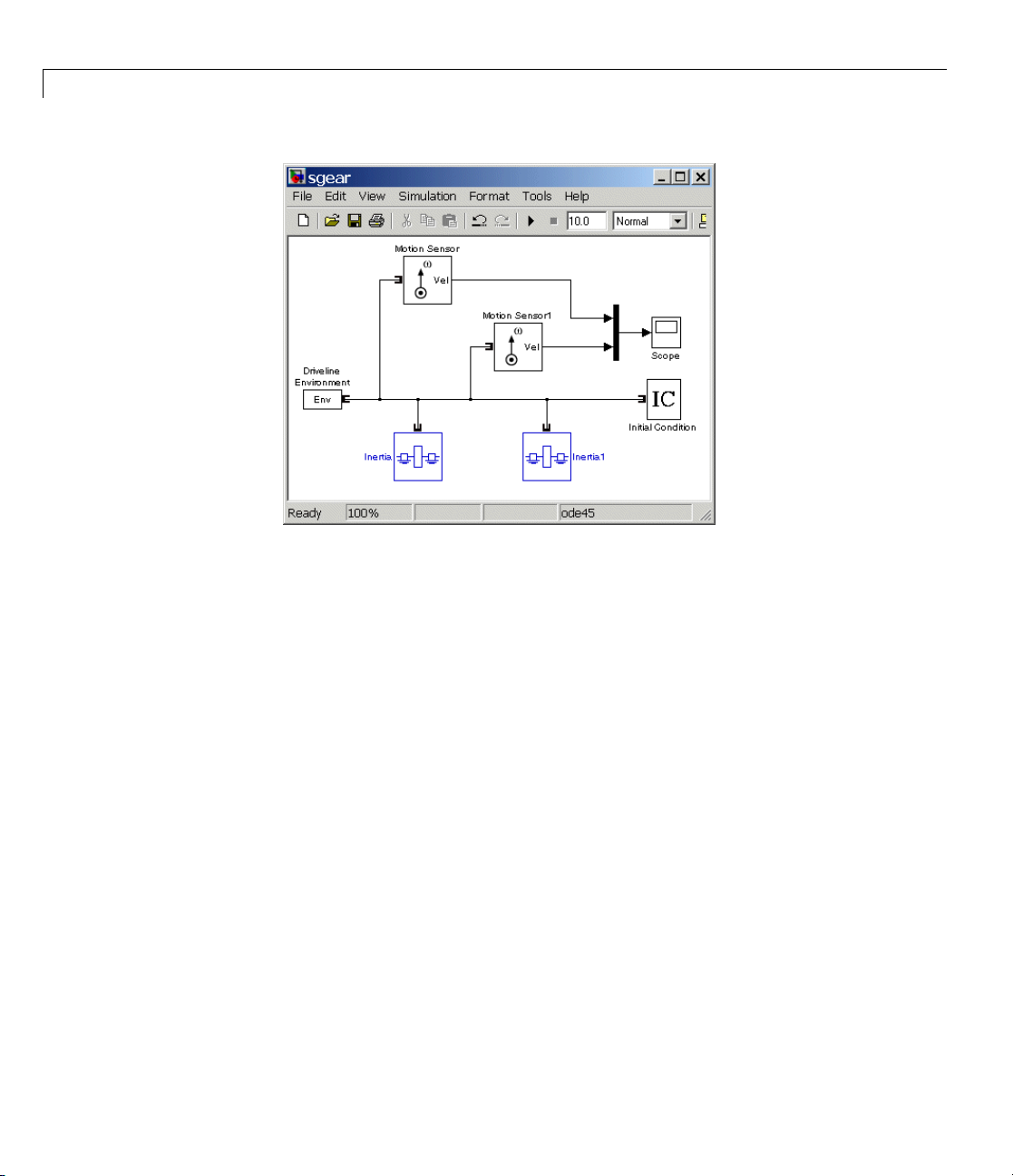
2 Simple Models

Two Spinning Inertias

2-12

4 Open the Initial Condition block. In the Initial angular velocity field,

replace its default

0 entry with pi radians/second (rad/s). Click OK.

If you do not connect an Initial Condition block to a driveline axis, the axis by default starts the simulation with zero angular velocity. You must ensure that the initial angular velocities of your coupled driveline axes are consistent with one another. If they are not, the simulation stops with an error.

5 Open the Scope block and start the simulation. The two angular velocities

are constant at 3.14 radians/second.

Coupling Two Spinning Inertias with a Simple Gear

Now you modify the model you just created by coupling the two spinning inertias with a simple, ideal gear with a fixed gear ratio.

1 From the SimDriveline block library, drag and drop a Simple Gear block

into your model. Open the block. Leave the default follower-base gear ratio value at check box and click OK. The simple gear then represents two gear wheels

2.CleartheFollower and base rotate in opposite directions

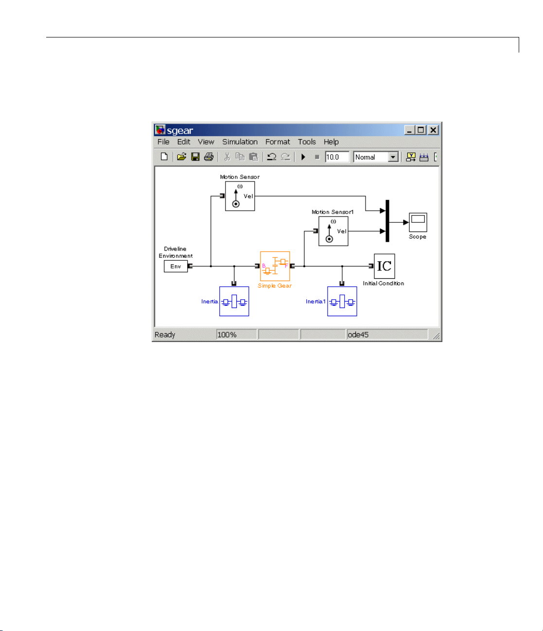
Representing and Transferring Driveline Motion and Torque

corotating in the sam e direction, with the sm aller wheel inside the larger. Reconnect the b locks as shown.

Two Spinning Inertias Coupled by a Gear

Leave the initial angular velocities at pi in the Initial Condition block. SimDriveline software automatically sets the correct initial angular velocity for Inertia.

2 Open the Scope and start the simulation. The two angular velocities

are constant at 3.14 and 6.28 radians/second for Inertia1 and Inertia, respectively. The fo llower-base gear ratio is 2, and the angular velocity of Inertia is twice that of Inertia1, with the same sign, because the two bodies are spinning in the same direction.

3 Now s

4 Restart the simulation. The two angular velocities are 3.14 and -6.28

elect the Follower and base r otate in opposite directions check

. The simple gear then becomes two w heels corotating in opposite

box

ections, with the two wheels meshed on their respective outer surfaces.

dir

radians for Inertia1 and Inertia, respectively. The second angular velocity

2-13

2 Simple Models

is twice the first and with opposite sign, because the two bodies are spinning in opposite directions.

5 Finally, again clear the Follower and base rotate in opposite

directions check box.

Torque-Actuating Two Coupled, Spinning Inertias

In the final version of the simple gear model, you actuate the inertias with an external torque instead of starting them with fixed initial angular velocities. The external torque varies sinusoidally. You can find a completed version of this model in the demo drive_sgear.

1 From the SimDriveline block library, copy a Torque Actuator and two

Torque Sensor blocks. From the Sim ulink block library, drag and drop a second Scope block, a second Mux block, and a Sine Wave block.

2 Disconnect the Inertia blocks from theSimpleGearandinserttheTorque

Sensors. Disconnect and delete the Initial Condition blo ck. The two axes will now default back to zero angular velocities.

2-14

Connect the other blocks as shown.

Representing and Transferring Driveline Motion and Torque

Two Spinn

3 Open both Scope blocks and start the simulation.

ing Inertias Coupled by a Gear and Actuated with Torque

The measured torques and angular velocities vary sinusoidally. The angular velocity of Inertia1 is half that of Inertia, as you saw in the previous models. But the torque in the second shaft is twice that in the first, as required by the laws of gear coupling.

If you select the Follower and base rotate in opposite directions check box in Simple Gear and restart the simulation, the same angular velocities and torques result, except that the values associated with Inertia1 and the second shaft are negative, because the second body and second shaft are spinning in opposite directions.

Sensing and Actuating Motion and Torque

The Sensor and Actuator blocks you use in the preceding mo de ls illustrate their dual nature: they act as driveline components themselves, but also let you connect drivelin e blocks with the rest of Simulink.

2-15

2 Simple Models

• Sensor & Actuator blocks have both driveline connector ports and normal

Simulink ports Simulink outports. You can actuate motion or apply external torques by feeding in actuation signals with a block’s Simulink inports.

Many other SimD r iveline blocks feature Simulink ports for inserting and measuring signals.

• You connect a Torque Sensor along a driveline axis, by placing it in series

with other driveline components.

• You connect the other Sensor and Actuator blocks across a driveline axis,

by branching the driveline connectionlineofftoonesideandconnecting this secondary line to the block; or by connecting the block to the end of adrivelineaxis.

>. You can extract sensor signal information with a block’s

Coupling Two Spinning Inertias with a Variable Gear

You can modify the simple gear model further by replacing the fixed-ratio gear with a gear whose gear ratio variesintime. Youspecifythegearratio variation with a Simulink signal. Start with the simple gear model you built in the preceding section or by opening and editing the drive_sgear demo.

2-16

1 From the SimDriveline block library, drag and drop a Variable Ratio Gear

block and replace the Simple Gear block with it. Open Variable Ratio Gear and ensure that the Follower and base rotate in opposite directions check box is selected (the default). The two shafts will spin in opposite directions.

2 The Variable Ratio Gear block accepts the continuously varying gear ratio

as a Simulink signal through the extra inport labeled create a S i m ulink signal f or the gear ratio with a Signal Builder block from the Sim ul ink block library . Build a signal that rises with consta n t slope from 1 to 2 over 10 seconds. Then connect the Signal Builder block to the

r port.

r. For this ex ample,

Representing and Transferring Driveline Motion and Torque

Simple Variable Ratio Gear Model

3 Leave the other, original settings of the simple gear m o del unchanged.

Open both Scopes and start the simulation.

The two shafts’ angular velocities and torques have opposite signs. Apart from this sign difference, the ratios of angular velocities and torques start at 1, because the initial gear ratio is 1. But as the gear ratio increases toward 2, the angular velocity of Inertia1 becomes smaller than that of Inertia, while the associated torque in the second shaft (apart from the opp osite s ign) becomes larger than that in the first shaft. Because of the changing gear ratio, the motion and the torques are no longer strictly sinusoidal, even though the actuating external torque is.

The drive_vgear demo is a full model of this type. To learn more about how to use variable gears, including the Coriolis acceleration, consult the Variable Ratio Gear block reference page.

Coupling Three Spinning Inertias with a Planetary Gear

You can further modify the simple gear model and use it as a starting point for studying more complex gear sets. One of the most important is the planetary gear, which has three wheels, the ring, the sun, and the planet, all held in place by a common carrier body. The planetary gear is inte resting in its own

2-17

2 Simple Models

right, but also important because it is a common component in complex, realistic transmissions.

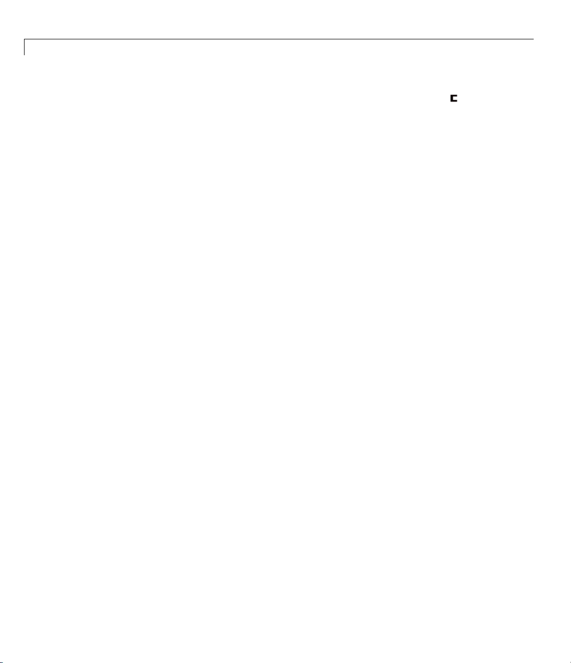
1 Replace the Simple Gear in your model with a Planetary Gear from the

SimDriveline block library. A planetary gear splits input angular motion from the carrier between the ring and sun wheels, each connected to their respective bodies.

2 Copy another Inertia and another Motion Sensor as well. Connect the

blocks to form the new diagram as shown.

2-18

Simple Planetary Gear Model

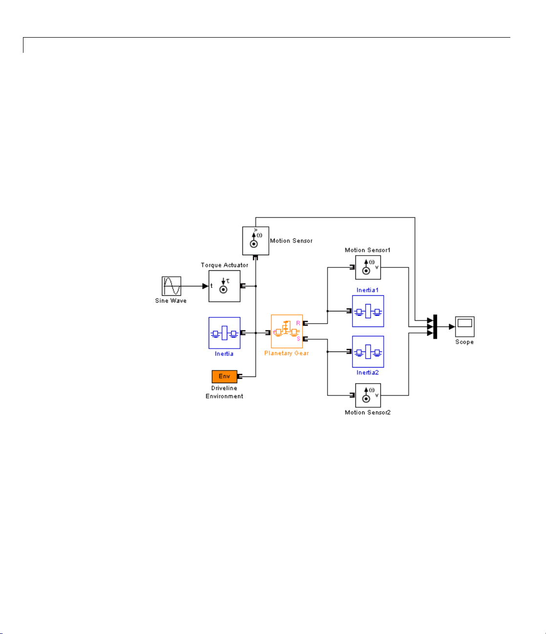
3 Enter 2 for the Ring/Sun gear ratio in Planetary Gear. Open the Scope

and start the simulation to observe the angular velocities of the ring, carrier, and sun, from largest to smallest. The ratio of the ring to sun gear velocities is always two.

Representing and Transferring Driveline Motion and Torque

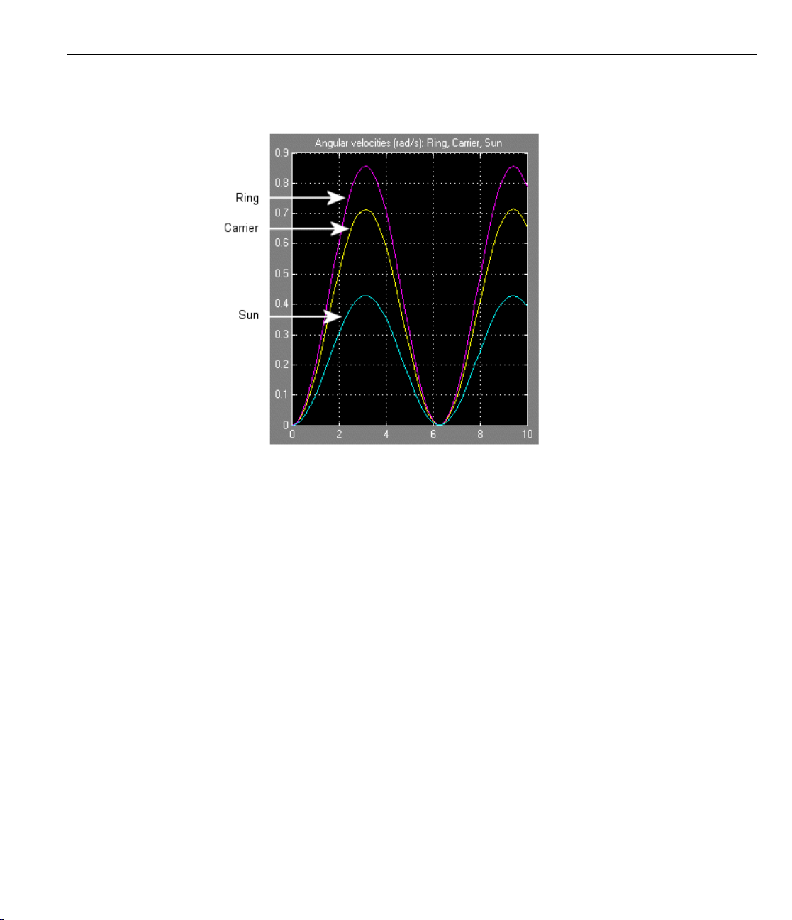
4 To see the ring and sun wheels spinning alone, you must lock the carrier.

In this case, you switch the torque actuation to the ring wheel. Copy a Housing block from the SimDriveline block library. Disconnect and delete Inertia, replacing it on the carrier driveline axis w ith Housing, and reconnect the Driveline Environment block to this connection line.

5 Insert a Torque Actuator and move the Sine Wave block next to it. Connect

it to the inport.

2-19

2 Simple Models

Simple Planetary Gear Model with Locked Carrier

2-20

6 Open the Scope and start your model. Observe the angular velocities of

the ring, carrier, and sun.

Representing and Transferring Driveline Motion and Torque

The carrier, connected to Housing, does not move. The ring is driven with a sinusoidal torque, and the sun responds by spinning in the opposite direction (ring and sun g ear wheels are external to one another) at tw ice the rate. The ring wheel has twice the radius (or twice the number of teeth) as the sun, so itspinshalfasfast.

To learn more about modeling planetary gears, see the Planetary Gear block reference page.

2-21

2 Simple Models

Actuating Drivelines with Torques and Motions

In this section...

“About Torques, Motions, and Actuation” on page 2-22

“Modeling the Effect of a Variable Inertia” o n page 2-24

“Actuating a Driveline with Torques” on page 2-25

“Actuating a Driveline with Motions” on page 2-26

“Setting the Motion Initial Conditions of a Driveline” on page 2-26

About Torques, Motions, and Actuation

A SimDriveline simulation solves, from the torques applied to spinning inertias, a driveline’s dynamics for its motions. H ow ev er, it can also accept motions imposed on a driveline and solve for the torques needed to produce those motions. A driveline simulation is typically a mixture of these two requirements, solving dynamics both forward (torque to motion) and inverse (motion to torque). Imposing motions and applying torques are together forms of driveline actuation.

2-22

This section discusses actuating drivelines with time-varying inertias, torques, motions, and motion initial conditions. All of these actuation types (except for initial conditions) require input Simulink signals to define time-varying functions.

Torque and Motion Actuation are Complementary and

ally Exclusive

Mutu

In all cases, you should exercise care as you apply a mixture of actua tion s to a driveline and its degrees of freedom (DoFs), as discussed in greater detail by the section, “Analyzing Degrees of Freedom” on page 3-14. The complete effect of the actuations must be such that

• Driveline DoFs actuated by torques are not also subject to motion

actuations. (They can be subject to motion initial condition actuation.)

• Driveline DoFs actuated by motions are not also subject to torque

actuations.

Actuating Drivelines with Torques and Motions

For a SimDriveline model to successfully simulate nontrivial motion, torque and motion actuations must exactly complement one another to account consistently for the motion of all the DoFs, no more and no less. If this criterion is not satisfied, one of these outcomes results.

• The motion of the driveline is trivial, staying in its initial motion state for

the entire simulation.

• The actuations are inconsistent with each other, and the simulation stops

with an error.

• The actuations leave the driveline underdetermined or overdetermined,

and the simulation stops with an error.

For more about driveline simulation errors, see “Troubleshooting Simulation Errors” on page 3-11.

Stabilizing Numerical Derivatives in Actuator Signals

To actuate a phys ical system m od eled by blocks, you often need to differentiate an incoming Simulink actuation signal.

Simulink provides a Derivative block for numerical differentiation of a signal. However, this block’s output is sometimes not stable or accurate enough for Physical Modeling purposes. Recommended alternatives to the Derivative block include the following.

Integrating Higher Derivative Signals. Start by specifying the highest derivative signal (such as an acceleration), then integrate this signal to obtain lower derivative signals (such as a velocity) using the Integrator block.

Transforming Signals with Transfer Functions. To differentiate a signal, use a transfer function block (Transfer Fcn). This block actually performs a Laplace transform convolution to smooth the output, which is not exactly the derivative.

You can eliminate this drawback by filtering the original signal f,then defining exact derivatives dF/dt, etc., of the filtered signal F by adding higher orders to the transfer function numerator. The order of the denominator should be equal to or greater than the number of output signals. Use the filtered signal F (instead of f), as well as the filtered derivatives.

2-23

2 Simple Models

In this example, the constant τ represents a smoothing time. The transfer functions define a filtered signal and its first derivative, two signals in all. Therefore, the transfer function deno minator should be seco nd order or high er.

Modeling th

You cannot However, y Ratio Gear momentum

1 Place a Va

2 Connect this constant Inertia to the Gear’sbase(B)orfollower(F)port.

3 Vary the gear ratio of the Variable Ratio Gear with an incoming Simulink

signal.

By changing the gear ratio, you change the effective inertia on the shaft from the constant Inertia.

• Effective inertia = (constant inertia)•(variable gea r ratio)

if the B port is connected to Inertia

• Effective inertia = (constant inertia)/(variable gear ratio)

if the F port is connected to Inertia

e Effect of a Variable Inertia

vary the inertia value of an Inertia block during a simulation.

ou can model a time-varying inertia indirectly with a Variable

block. This method relies on the conservation of angular

riable Ratio Gear between a shaft and an Inertia.

2-24

Actuating Drivelines with Torques and Motions

Effective Variable Inertia with a Variable Ratio Gear

Actuating a Driveline with Torques

You can apply a torque to a driveshaft

• Directly, with a Torque Actuator block

• Indirectly, with a block that generates torque, using a Torque Actuator as

part of a larger subsystem. Such blocks include:

- Dynamic elements such as clutches, torque converters, and engines

- Transmissions, which contain clutches

In any case, a Torque Actuator accepts an incoming Simulink signal and originates, from its driveline connector port, a driveline connection l in e carrying that torque.

The SimDriveline simu la t ion so lves for the motion of the spinning driveshaft, given the torque it is subject to. Therefore you cannot, in addition, subject that same driveshaft to motion actuation.

2-25

2 Simple Models

Caution A driveline actuated by a torque must have a nonzero inertia,

represented by one or more connected Inertia blocks. A torque-actuated driveline without any inertia experiences a singular acceleration. In this case, the SimDriveline simulation will stop with an error.

Actuating a Driveline with Motions

You can apply a motion to a driveshaft directly, with a Motion Actuator block.

A Motion Actuator accepts an incoming Simulink signal and originates, from its driveline connector port, a driveline connection lin e spinning with the specified motion.

TheSimDrivelinesimulationsolvesforthetorquecarriedbythespinning driveshaft, given its motion. Therefore you cannot, in addition, subject that same driveshaft to torque actuation.

2-26

Setting the Motion Initial Conditions of a Driveline

When driveline simulation starts, the c omplete driveline determines the initial motion of all dri veshafts by a combination of constra in ts, motio n actuators, and initial condition actuators. If, after the application of the complete driveline’s con strai nts and actuators, one or more of the driveshaft motions remain undetermined, these driveshafts start simulation with zero angular velocity by default.

You can exercise direct control over how a driveshaft starts motion during simulation by connecting it to an Initial Condition actuation block. You set the initial velocity of the driveshaft in the block’s dialog.

For more about constraints and degrees of freedom, see “Analyzing Degrees of Freedom” on page 3-14.

Actuating Drivelines with Torques and Motions

Caution You must ensure that whatever initial conditions you impose on the driveshafts in yo ur driveline are consistent with all of the driveline’s constraints and motion actuators. If an inconsistency occurs, the SimDriveline simulation stops with error.

Resolving Undetermined Motions in Complex Gears

A simple gear has two ports and imposes one constraint between them, leaving one independent DoF. Once one port is connected to a driveshaft, the motion of the other port’s driveshaft is determined.

A complex gear has three or more ports and imposes one or more constraints among them. A complex gear can have any number of independent DoFs, including none.

For more about complex gears, see “Representing and Transferring Drivel ine Motion and Torque” on page 2-9.

Tip If a simulation apportions the initial motions of a complex gear in an unsatisfactory way, determine how you want the overall initial motion divided up and enforce that division with one or more Initial Condition blocks on one or more of the complex gear shafts.

However you divide the initial motion among the gear shafts, ensure that this division is consistent with all constraints in your driveline, as well as any motion actuators.

2-27

2 Simple Models

Controlling Gear Couplings with Clutches

In this section...

“About M otion, Gears, and Clutches” on page 2-28

“Engaging and Disengaging Gears with Clutches” on page 2-28

“Modeling Re alistic Clutch Systems with Loss” on page 2-34

“Braking Motion with Clutches” on page 2-37

“Modeling Friction Clutches a t a F undamental Level” on page 2-41

About Motion, Gears, and Clutches

The most important requirement of a practical drivetrain is the ability to transfer rotational motion and torque among spinning components at different speeds and gear ratios. A single set of gears is usually not sufficient to accomplish this. Clutches are the critical components that allow the drivetrain to selectively transfer mot ion and torque at different gear ratios under manual or automatic control.

2-28

This section e xplains how to model and use clutches in driveline models without and with frictional losses and braking.

Engaging and Disengaging Gears with Clutches

A common problem in drivetrain design is transferring motion and torque at different fixed gear ratios. Drivetrains are typically designed to switch among a set of discrete gear ratios. Implementing the switch from one gear ratio to another requires gradually disengaging one set of driveline couplings and engaging another set. Clutches allow you to gradually engage and disengage driveline shafts from one another.

The Controllable Friction Clutch block represents a standard surface friction-based clutch that models this behavior and requires no more than modest preparation to use. This section uses this block. You also can model clutches in greater detail u sing the Fundamental Friction Clutch block, which requires you to specify the static and kinetic clutch friction more completely. See “Modeling Friction Clutches at a Fundamental Level” on page 2-41.

Controlling Gear Couplings with Clutches

Tip You can model continuous motion-torque transfer with the Torque Converter block, which simulates fluid viscosity instead of surface friction and which never locks.

How a Clutch Works

A clutch makes two shafts spinning at different rates spin at a single rate by applying forces that tend to accelerate one shaft and decelerate the other. The most common way for a clutch to accomplish this is with surface friction. Such a clutch can operate in one of three modes of motion:

• Disengaged: the clutch applies no friction at all.

• Engaged but unlocked: the clutch applies kinetic friction, and the two

shafts spin at different rates.

• Engaged and locked: the clutch applies static friction, and the two shafts

spin together.

A clutch consists of mated frictional surfaces overlapping one another and connected on either side to a shaft. If the clutch is disengaged, the frictional surfaces have no contact and the shafts spin independently. To engage the clutch, a moderate amount of contact between two surfaces is induced by applying clutch pressure (a force normal to the surfaces). The two surfaces in contact and moving relative to one another experience kinetic friction, which causes them to narrow their relative velocity. The faster surface tends to slow down (unless an external torque is acting) and the slower one to speed up. At some critical combination of reduced relative speed and pressure (normal force), the clutch locks, so that the two shafts are spinning at the same rate. The locking of the shafts is controlled by static friction, which holds the shafts together as long as sufficient normal force is applied and no relative torque is large enough to overcome the locking. If the clutch unlocks but is still engaged, it again applies kinetic rather than static friction.

2-29

2 Simple Models

Note The transition between unlocked and locked states is discontinuous.

Modeling a clutch locking or unlocking requires searching for the correct combination o f pressure and torque acting on the clutch.

The locking and unlocking are determined during simulation by accurate zero-crossing detection and repeated mode iteration. In the default case, this mode iteration induces algebraic loops in Simulink, non-time-based simulation steps that trigger warnings at the MATLAB command line. You can change this default behavior through your driveline’s Driveline Environment block.

Engaging and Disengaging a Gear with a Clutch

Here you construct a simple model that simulates a gear being engaged, then disengaged, by a clutch. Torque and motion are transferred from one s haft to another over a finite time interval. Start with the simple gear model of the last section or with the drive_ sge ar demo. The completed clutch model is the drive_sclutch demo.

2-30

1 From the SimDriveline block library, you need a Controllable Friction

Clutch block. Also copy a Signal Builder and a Constant block from the Simulink block library.

2 Remove the Torque Sensor blocks, insert the Clutch between Inertia1 and

Simple Gear, then reconnect the connection lines.

3 In the Clutch dialog, select the Output clutch mode check box, but leave

the other defaults. Rearrange and connect the blocks as shown here.

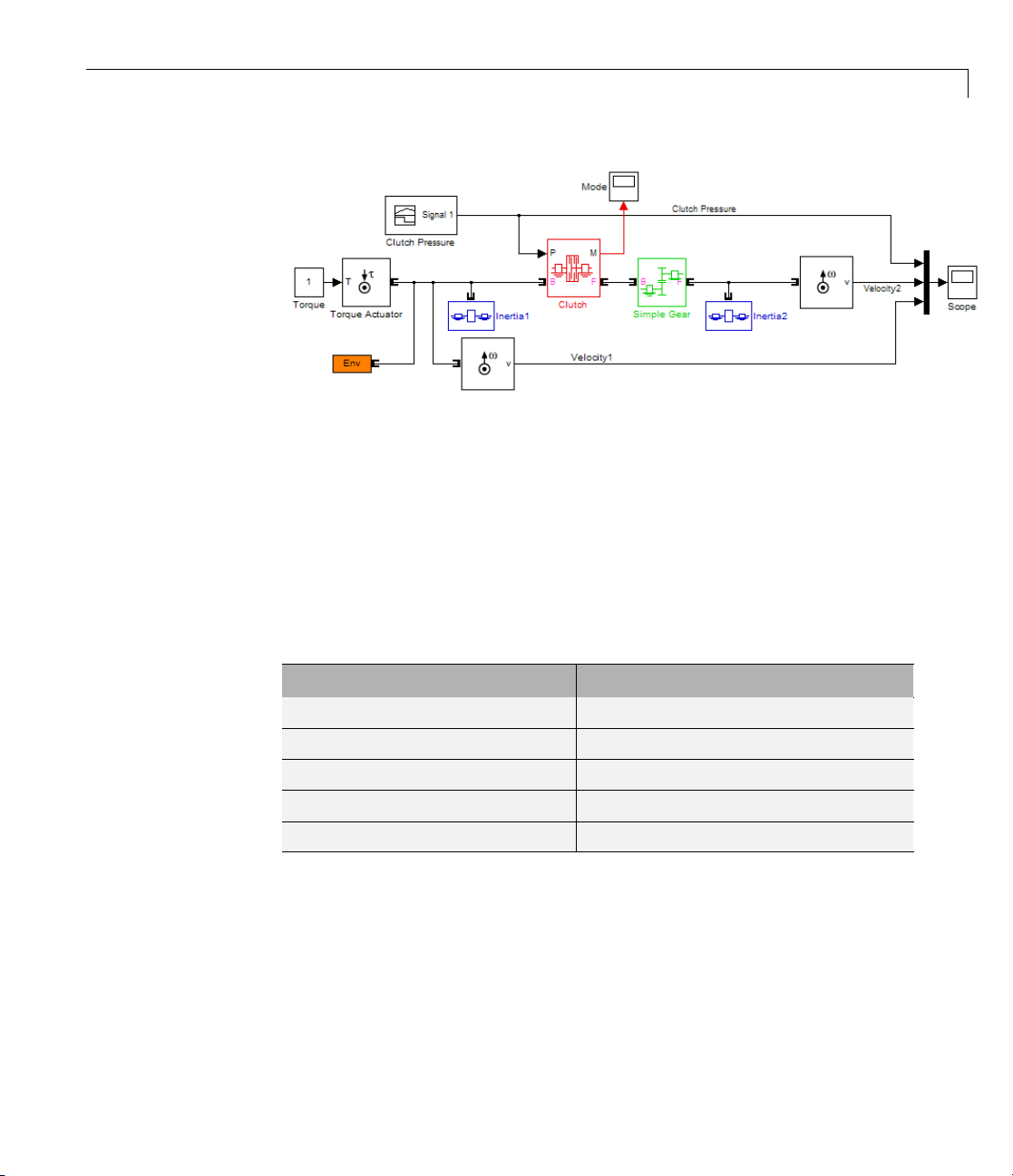
Controlling Gear Couplings with Clutches

Simple Clutch Model with Programmed Clutch Pressure

4 Use the Constant block as the input torque signal in place of the sinusoidal

signal. Reconfigure Mux and the first Scope blocks to accept three signals, the two angular velocities and the clutch pressure. Connect the second ScopetodisplaytheClutchmodesignal.

5 Open Signal Builder and construct the following signal. Signal Builder

specifies the clutch pressure signal, which is normalized between 0 and

1. (The Peak normal force field in Clutch determines the maximum clutch pressure.)

Time Range (Seconds) Signal Value

0–2 0

2–4

0–0.8withconstantslope

4–6 0.8

6–7

0.8–0withconstantslope

7–10 0

6 Open the Scopes and start the simulation.

The normalized clutch pressure signal follows the profile you created in Signal Builder and determines the model’s behavior.

• From 0 to 2 seconds, the velocity of Inertia1 increases linearly because

it is subject to a constant torque.

2-31

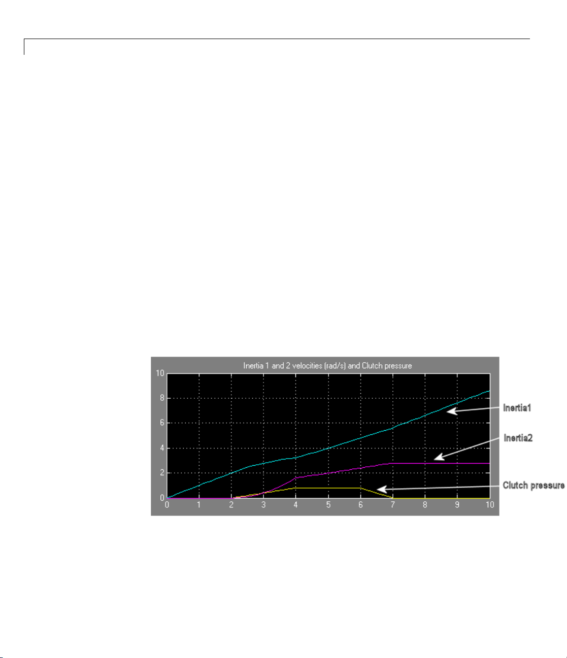
2 Simple Models

• At 2 seconds, the clutch begins to engage, and Inertia2 begins to spin. The

velocity of Inertia1 continues to rise, although at a slower rate, because the two inertias now share the external torque.

• At 4 seconds, the pressure reaches its maximum, and the clutch locks. The

driveshafts connected by the clutch spin together. Inertia1 and Inertia2 continue to speed up at constant accelerations.

• At 6 seconds, the clutch begins to disengage as the pressure drops. Inertia1

and Inertia2 continue to accelerate with the applied torque.

The clutch unlocks at 6.77 seconds and fully disengages at 7 seconds. (The clutch unlocks a little before completely disengaging because the pressure, even before vanishing, becomes too small to maintain the lock.) Inertia1 is still accelerating. But Inertia2 now freeofthedriveshaftanditstorque,no longer accelerates and instead spins at a constant rate without frictional loss.

While the two shafts are locked, between 4 and 6.77 seconds, Inertia1 and Inertia2 spin in a fixed 2:1 ratio. The Simple Gear, with a gear ratio of 2 between follower and base, transforms Inertia2’s velocity to half that of Inertia1.

2-32

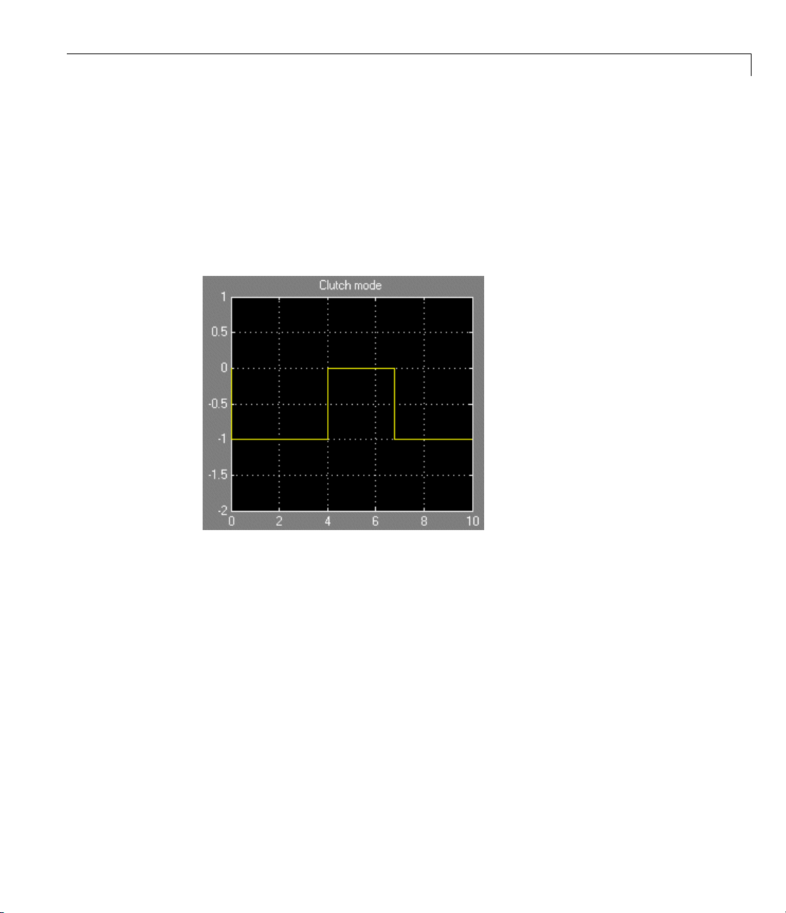
Controlling Gear Couplings with Clutches

How the Clutch Mode Indicates Locking and Unlocking. The Clutch mode signal indicates the relative motion of its two connected shafts. From 0 to 4 seconds, the two shafts are moving relative to one another. The follower (driven) shaft is slower than the base (drive) shaft, so the mode signal is -1. Once the two shafts lock, their relative velocity is 0, and the mode signal switches to 0. At 6.77 seconds, they u nl ock , and the drive (base) shaft starts accelerating faster than the driven (follower) shaft. The mode signal switches back to -1.

Engaging and Disengaging Driveshafts with a Clutch and Witho

To see the two Inertias of the preceding model locked and spinning at the same rate,

1 Remove Simple Gear and connect Inertia1 directly to the Clutch. Change

2 Rest

ut a Gear

the Peak normal force value in Clutch to

art the simulation. Inertia1 and Inertia2 now spin at the same rate

le the clutch is locked between 4 and 6.77 seconds.

whi

2.5 (ne w ton s ) .

2-33

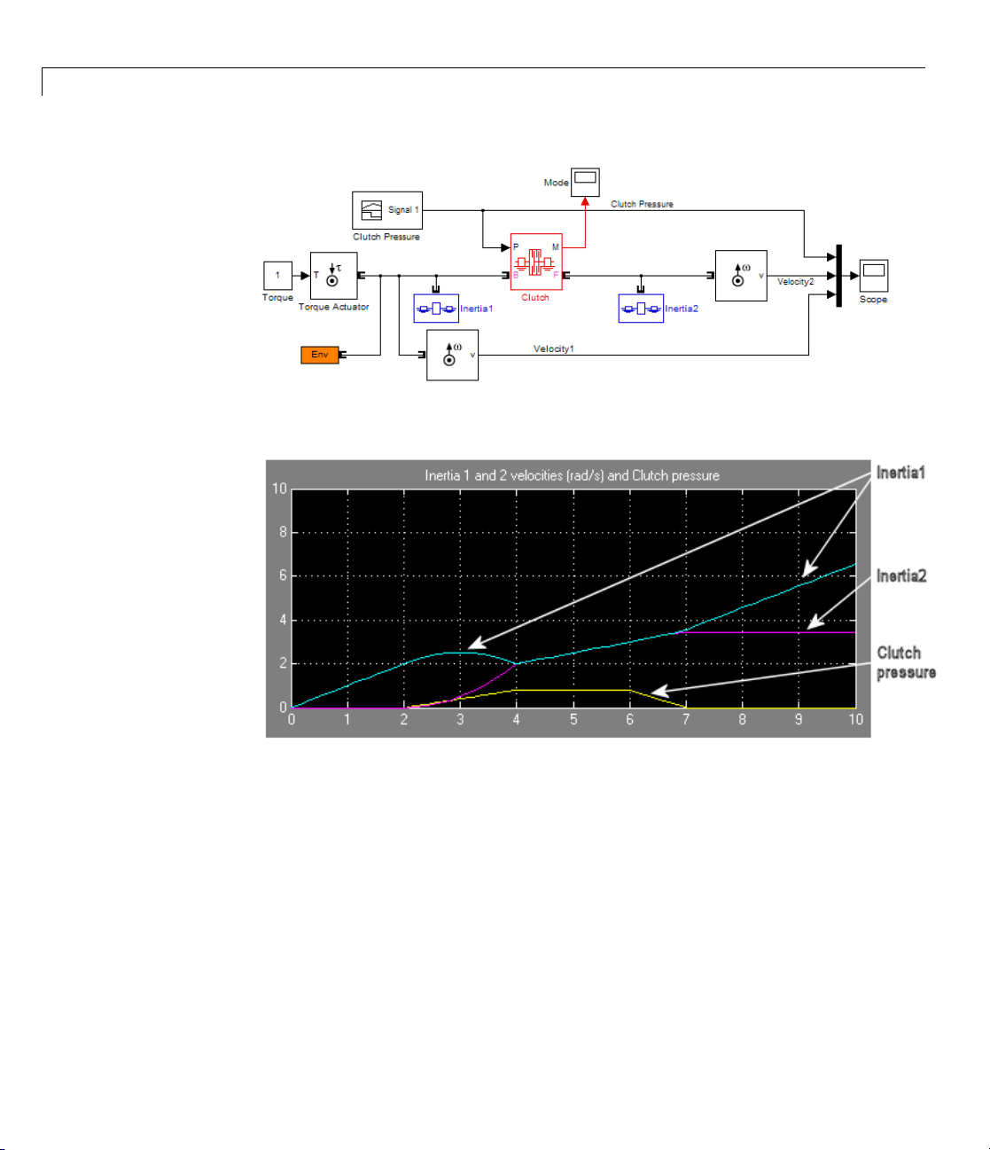
2 Simple Models

Simple Clutch Model with No Ge ar

2-34

Modeling Realistic Clutch Systems with Loss

To make your clutch system model more realistic, you should add frictional damping to the spinning shafts of drive_sclutch. Here you add a kinetic friction torque proportional to the angular velocity to both sides of the clutch. A simple way to do this is to create a friction subsystem that applies such a torque to any driveline axis it is connected to. Then you can copy the subsystem and m odify your existing clutch model by connecting the two copies on either side of the clutch.

Controlling Gear Couplings with Clutches

Tip The velocity used for this damping is the absolute velocity of a single shaft relative to rest (as defined by a Housing block, for example). If you had two driveline shafts and wanted to exert a relative damping between them as a function of their relative velocities, you could use the Torsional Spring-Damper b lock. In general, this block applies a mixture of spring-like and damping torques between the two connected axes. But you can apply a pure damping torque by simply settingthespringconstanttozero.

Creating a Torque Damping Subsystem

The frictional torque is τ constant. To apply the frictional torque proportional to the velocity, you need to

1 Measure the angular velocity of the driveline axis

2 Multiply it by -μ, because the frictional torque opposes the motion

=-μω,whereμ is the frictional proportionality

fric

3 Apply the resulting torque bac k to the dr iveline axis

To implement kinetic damping torque:

1 Copy Motion Sensor and Torque Actuator blocks and, from the Simulink

library, a Gain block, into your model window.

2 Connect the angular velocity port Vel to the inport of the Gain block and

the outport of the Gain block to the torque inport of the Torque Actuator block. Enter

-0.3 for the Gain value in the Gain dialog, leaving the other

defaults.

3 With your cursor, select the connected Sensor-Gain-Actuator block set, and

create a subsystem. Call it port appearing on its block is a driveline connector port port

Now create a second copy of

Damper. When you create the subsystem, the

, not a Simulink

Damper.

2-35

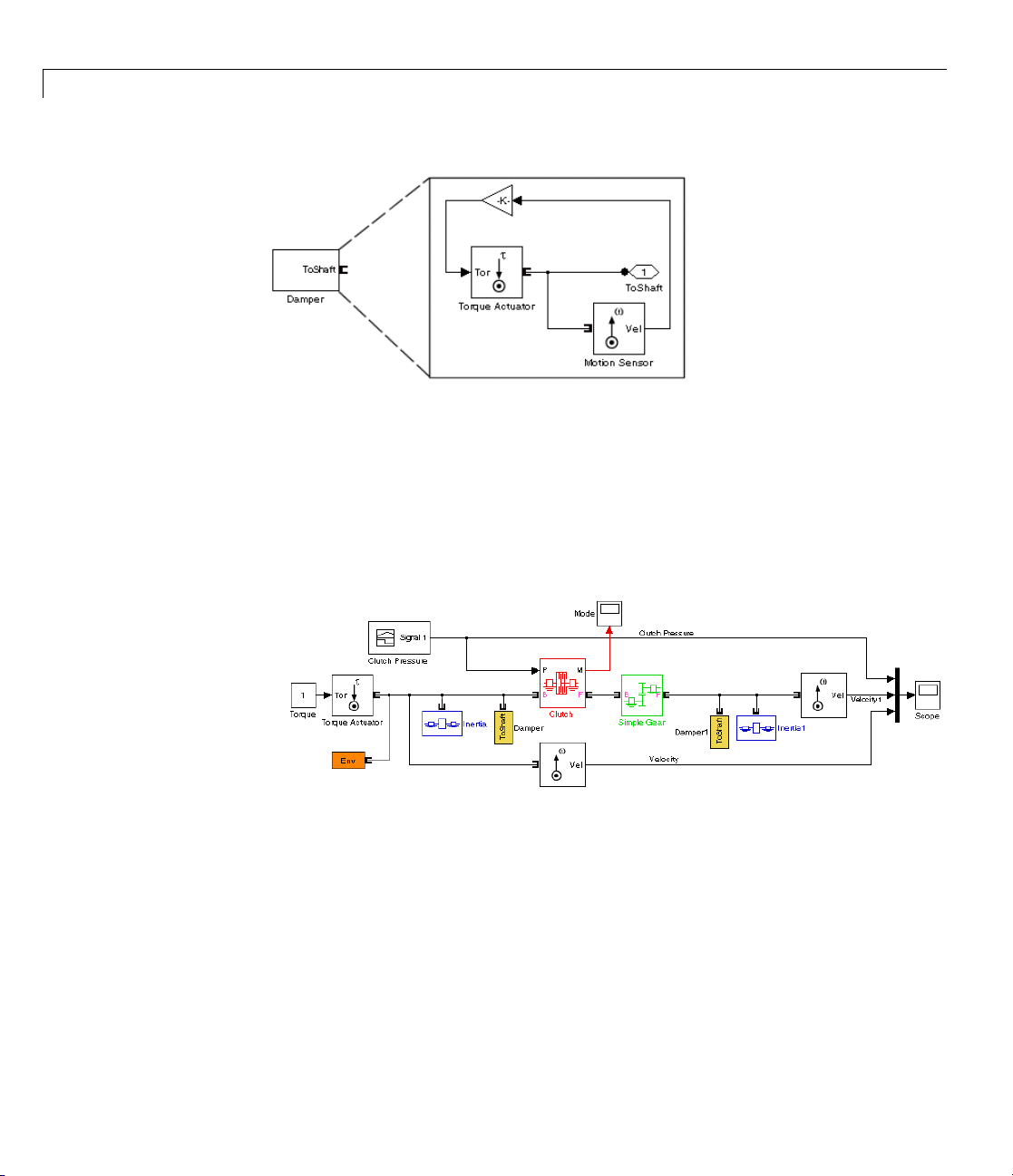
2 Simple Models

Rotational Kinetic Damping Subsystem

Connecting and Simulating the Damped Clutch S ystem

Complete and run the model.

1 Connect the two Damper subsystems to the driveline of your previous

clutch model as shown.

2-36

Damped Simple Clutch Model

2 Changethesimulationtimeto20seconds. ThenopentheScopeblocks

and click Start.

Readjust the horizontal axes of the Scopes with Autoscale to see the full plots. The clutch pressure and external torques are applied as before. But the shaft rotations are different now because of the damping.

Controlling Gear Couplings with Clutches

Inertia1, as before, begins to spin when the clutch starts to engage at 2 seconds. After the clutch locks at 4 seconds, the body continues to accelerate, but at a slower rate than it did without damping. At 6 seconds, the clutch begins to disengage and completely disengages at 7 seconds. Unlike the friction-free case, Inertia1, subject to friction, now starts to slow down. Its angular velocity d rops exponentiallywithtimeoncetheexternaltorque is removed.

The behavior of Inertia is more complex. It begins to spin up, but at a lower rate than before, because of the damping. Between 2 and 7 seconds, Inertia has to share the external torque with Inertia1 via the Clutch and the Simple Gear. After seven seconds, the external torque applies to Inertia alone. It continues to accelerate, but at an ever-slowing rate, because of the damping. If you let the simulation run without stopping, Inertia will approach its terminal angular velocity, a state where the frictional torque exactly balances the externally applied torque. The terminal velocity is ω

term

= τ

/μ or 1/0.3 =

ext

3.3333 radians/second in this case. The Scope plot shows this terminal value.

Braking Motion with Clutches

A special case of transferring motion occurs when you want to brake the spinning of a driveline component, slowing it down until it stops. The common way to brake the motion is to couple the spinning component to a fixed housing, which effectively has infinite inertia and is represented by a SimDriveline Housing block. Because the housing cannot move, a driveline

2-37

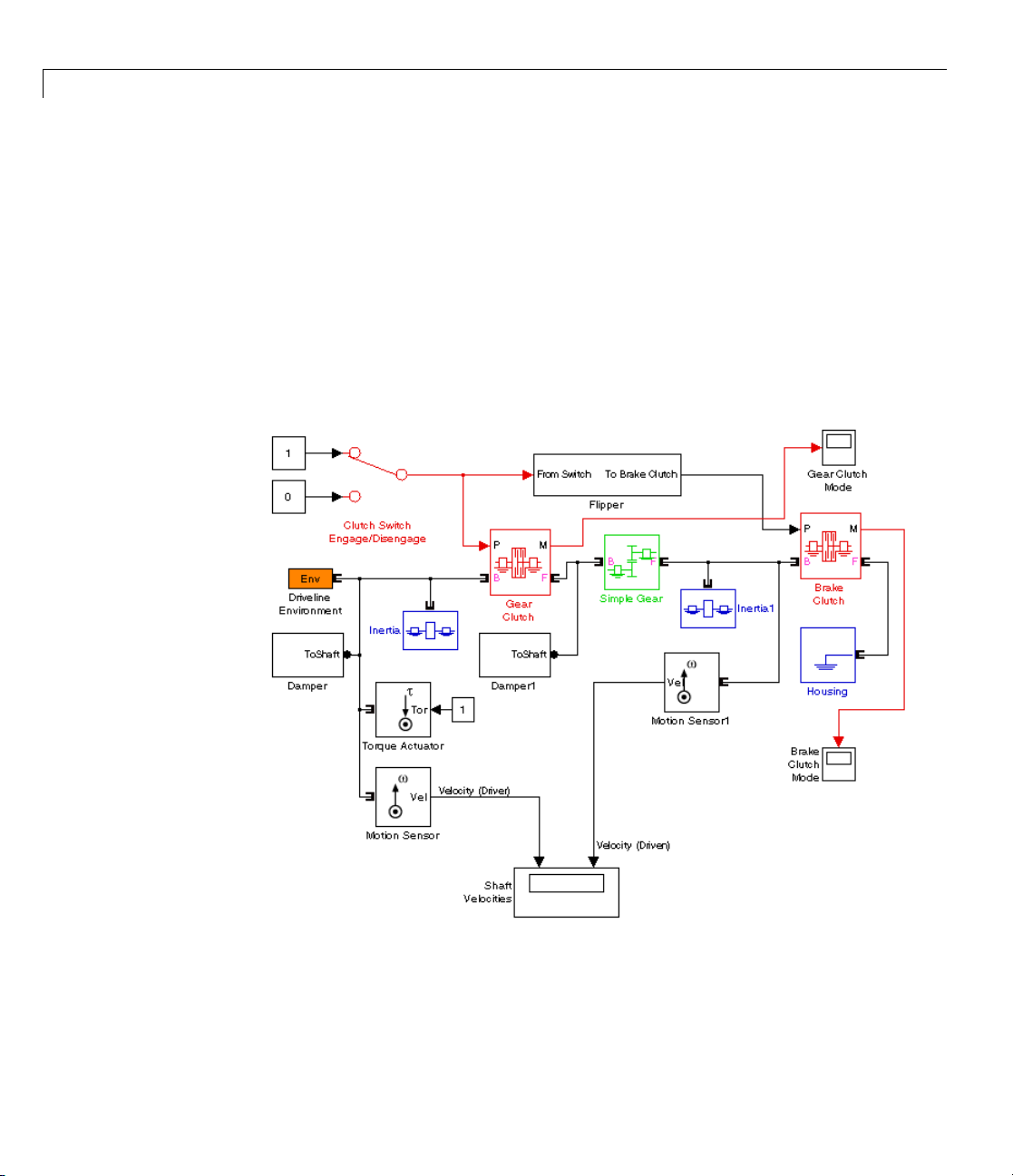
2 Simple Models

axis locked to a housing also cannot move. You can implement the gradual engagement or disengagement of a driveline component with a housing using a clutch, just as you use a clutch to gradually couple or uncouple two spinning shafts.

Braking with a Double-Clutch System

The drive_clutch_engage demo model is an elaboration on the preceding models of this chapter and features two clutches, one of which acts as a brake. The model also includes frictional damping for greater realism. The simulation time is set to

inf (infinity).

2-38

ple Clutch Model with Brake Clutch

Sim

is model again uses the basic structure of inertia-clutch-gear-inertia.

efirstbody,Inertia,isstilldrivenby an external torque, and the initial

Controlling Gear Couplings with Clutches

velocities are still 0. There is, however, another clutch for the second body, Inertia1, that can couple Inertia1 to the Housing and bring it to a stop. Another new feature, compared to the preceding models, is the switching assembly made of the Clutch Switch and Flip per blocks. You can flip this switch to apply a constant clutch pressure signal to either Gear Clutch or Brake Clutch. The two Damper subsystems are identical to those you constructed in “Modeling Realistic Clutch Systems with Loss” on page 2-34, except that the frictional constants, the Gain values of the Gain blocks, are set to

-0.1.

1 Start the model with the Clutch Switch set to 1. T he clutch pressure is

then applied to Gear Clutch, which engages and locks the driver and driven shafts and causes Inertia and Inertia1 to rotate together.

The angular velocity of Inertia1 (2.5 radians/second) is half that of Inertia (5 radians/second) because the gear rat io of the Simple Gear block is 2, follower to base. In this switch mode, no clutch pressure is applied to Brake Clutch, which remains unengaged. The mode of Brake Clutch is then -1, because Brake Clutch’s follower, the Housing block, is at rest, while the base, Inertia1, is spinning. The mode of Gear Clutch is 0, because its base and follower, the driver and driven shafts, are locked together.

After an initial transient, the system settles into a steady state of motion where the external torque is exactly balanced by the frictional losses. The effective frictional constant, with two dampers, is 0.2. With an external torque of 1 newton-meter, the terminal angular velocity of Inertia is then ω = 1/0.2 = 5 radians/second.

2 With the simulation running, n ow change the Clutch Switch to 0 to

disengage Gear Clutch and engage Brake Clutch. The system undergoes another transient while Gear Clutch disengages and Brake Clutch engages.

The angular velocity of Inertia and the driver shaft settles down to a new steady state of 10 radians/second, twice its old speed. The mode of Gear Clutch is now -1, because the driven shaft (follower) is not moving, while the driver shaft (base) continues to spin.

Because Gear Clutch is now disengaged, Inertia is no longer subject to the second frictional damping block, Damper1. The effective frictional constant drops in half, to 0.1, and the terminal velocity doubles. At the same time, Inertia1 is no longer receiving torque through Gear Clutch. But

2-39

2 Simple Models

Brake Clutch is engaged and couples Inertia1 to the immobile Housing. Once engaged, the kinetic friction of Brake Clutch and Damper1 bring the driven shaft and Inertia1 to a stop. Because it locks, Brake Clutch’s mode becomes 0.

To see the transient behavior at simulation start and when you switch the clutches,

1 Start the simulation and let it run for a short time. Then switch Clutch

Switch to the other mode.

2 After another short time, stop the sim ulation. Use the Autoscale feature

of the Scopes to capture the entire simulation sequence. The transients from the starting behavior and the switching transition will be visible.

For example, in these plots, the model was started with Clutch Switch set to 1 (Gear Clutch locked, Brake Clutch disengaged, no braking). The velocities quickly climbed to their steady-state values. Then Clutch Switch was changed at about 682 seconds of simulation time. Gear Clutch disengaged and Brake Clutch engaged, braking the driven shaft. The driver shaft’s angular velocity rose from 5 to 10 radians /seco n d. The driven shaft’s angular velocity dropped to 0.

2-40

Controlling Gear Couplings with Clutches

Modeling Fricti

The Controllabl normalized pres other characte

Modeling a fri the kinetic an gives you that external sig friction and

e F riction Clutch block is easy to use, requiring only a single

sure signal to modulate the kinetic friction. You fix all its

ristics before starting simulation.

ctionclutchatafundamentallevel requires direct control over

d static friction torques. The Fundamental Friction Clutch block

greater control. With this block, you must specify, by either

nals or internal sensor-actuator feedback, the clutch’s kinetic

static friction limits (positive and negative) as functions of time.

on Clutches at a Fundamental Level

2-41

2 Simple Models

Combining Clutches and Gears into Transmissions

In this section...

“About G ears, Clutches, and Transmissions” on page 2-42

“Modeling a Simple Two-Speed Transmission with Braking” on page 2-43

“Introducing the Transmission Templates Library” on page 2-50

“Modeling a CR-CR 4-Speed Transmission Driveline with Braking” on page 2-51

About Gears, Clutches, and Transmissions

In a real drive train, you coup le an input or drive shaft to one of many output or driven shafts, or to one driven shaft with a choice of several gear ratios. Thedrivetrainthenrequiresseveralclutches to switch between gears. You couple one of the driven shafts or one of the gear sets by engaging one of the clutches. You then sw itch to another output shaft or another gear ratio by disengaging one clutch and engaging another.

2-42

You can also engage more than one clutch at a time to use multiple gear sets simultaneously. Realistic transmissions engage multiple gear sets at the same time to produce a single effective gear ratio, or drive ratio. Changing gears requires disengaging one set of clutches and engaging another set. You specify the set of clutches to engage and disengage for each desired gear ratio in a clutch schedule. Designing a clutch schedule and shaping and sequencing the clutch pressure signals frequently constitute the most difficult part of transmission design. A realistic transmission model must also include losses duetofrictionandimperfect gear meshing.

This section explains how to model transmissions, first by creating a transmission mo del from g ears and clu tches, then by using the SimDriveline library of predesigned transmission subsystems. One such predesigned transmission, the CR-CR 4-speed transmission, is the basis of another example.

Combining Clutches and Gears into Transmissions

Note The examples in this section contain unrealistic clutch pressure signals that rise and fall sharply. A realistic transmis sio n is controlled by clutch pressure signals that rise and fall s m oothly. For a car demo with smoothed clutch pressure signals, see “Modeling and Simulating a Complete Car” on page 2-58. “Improving Performance” on page 3-5 discusses the relationship of sharp and smooth clutch pressure signals to the Simulink solver choice and settings.

Modeling a Simple Two-Speed Transmission with Braking

The demo model drive_strans_ideal contains a driveline system that makes up a simple but complete transmission.

Simple Transmission with Two Gear-Clutch Pairs and Braking

2-43

2 Simple Models

The model is an elaboration of the drive_clutch_engage demo model presented in “Braking Motion with Clutches” on page 2-37. This model also contains two driveline shafts or axes, with an actuating torque applied to the driven shaft. Both the driver and the driven shafts are subject to, respectively, large and very small kinetic damping torques. (The kinetic to rqu e constants μ are

0.1 and 10 In the steady state, the driving and damping torques balance one another, and the two shafts spin at constant rates. (If braking is engaged, the driven shaft is stopped, as before.) But there are now two selectable gears to couple the two axes, instead of one.

This transmission model couples the gears in a simple way, with each gear and the brake associated with its own respective clu tch . Coupling one gea r requires engaging and locking its corresponding clutch, while ensuring that the other two clutches are disengaged. Switching on the brake requires disengaging the two gear clutches and locking the brake clutch.

-4

newton-seconds/radian, respectively, in Damper1 and Damper2.)

Setting Up the Gears, Clutches, and Brake

The two gears are Simple Gear blocks with different gear ratios, each connected in series with its corresponding clutch. The two gear-clutch pairs are coupled in parallel, and this parallel assem bly then cou ples the driv er shaft to the driven shaft, with their two spinning inertias. One gear is a “low” gear, the other a “high” gear. The “low” and “high” labels, following common usage for automobile gears, refer, not to the gear ratios, but the angular velocity ratios.

2-44

Caution The ratio of speeds in a gear is the reciprocal of the gear ratio.

• The “low” gear is the Simple Gear 5:1 block, which can be coupled by

engaging its corresponding clutch, modeled by the Lo Gear Clutch block. The gear ratio is 5:1, so that the ratio of output to input (follower to base) angular speeds is 1/5. Hence the name “low gear.” Such a gear, by the same token, has a high torque transfer ratio of 5, from base to follower. In an automobile, a “low” gear like this is used to accelerate the vehicle from a stop by transferring a large torque down the drivetrain from the engine.

• The “high” gear is the Simple Gear 2:1 block, coupled by engaging its own

clutch, represented by the Hi Gear Clutch block. The gear ratio is 2:1, and

Combining Clutches and Gears into Transmissions

theangularvelocityratiooffollowertobaseis1/2,or5/2timestheratioin the“low”gear. Hencethename“highgear.”Thetorquetransferratiois only2frombasetofollower. Anautomotive “high” gear is used for milder acceleration or coasting once a vehicle is moving at a significant speed. The vehicle acceleration generated by this gear is less than that generated by the “low” gear.

While either Gear Clutch is engaged, the Brake Switch is disable d. Yo u can start braking and bring the driven shaft to a stop by engaging Brake Clutch. This clutch, once locked, holds the driven axis fixed relative to the Housing. The driver shaft contin ue s to spin, subject to the competing driving and damping torques. In this transmission, the brake is completely disabled if either gear clutch is engaged. Disengaging the gears puts the transmission into “neutral” and allows you to use the Brake Switch to apply or not apply brake clutch pressure.

Clearly, this simple transmission is based o n mapping each transmission state one-to-one with an engaged clutch. You cannot engage more than one clutch at a time without creating conflicts between gear ratios or between the driver shaft and the Housing. In a real tr ansmissio n, such conflicts generate internal stresses and might destroy the driveline. Such conflicts cause a SimDriveline simulation to stop with an error.

Controlling the Transmission State with a Clutch Schedule

The requirement to engage a certain clutch or set of clutches and disengage others, both to implement transmissio n functions and to avoid motion conflicts between gears, is the basis for all clutch schedules. Simulink provides a number of ways to implement clutch schedules, depending on the complexity of the transmission and how much realism you require for the clutch pressure signals.

Warning You must check every transmission’s clutch schedule to implement the various transmission states correctly and to avoid motion conflicts among gear sets. You must also check clutch pressure signal profiles to make sure that any transmission’s clutches are engaged, locked, unlocked, and disengaged in a realistic and conflict-free manner. Unphysical or conflicting clutch schedules and clutch pressure signals lead to SimDriveline simulation errors.

2-45

2 Simple Models

Avoiding such conflicts leads, for the drive_strans_ideal model, to a unique clutch schedule.

Clutch Schedule for the Simple Two-Speed Transmission

Transmission State

Neutral/Braked

Low Gear

High Gear

The model contains a simple Clutch Control subsystem to implement the clutch schedule and to output (or, in the case of the brake, enable) the clutch pressure signals to lock each clutch as needed.

h Control Subsystem for Simple Transmission Model

Clutc

is simplified and unrealistic clutch control model, the clutch pressure

In th

als are just constants: 1 to engage and lock a clutch, and 0 to disengage it.

sign

utch pressure signal is normalized to equal 1 when the surface friction

(A cl

e equals the peak normal force specified in the Controllable Friction

forc

tch dialog.) The brake signal is not a pressure, but only an enabling signal

Clu

the Brake Switch in the main model. The table of these constants, for

for

h transmission state, is contained in the Clutch Schedule Table block,

eac

tomized from the Simulink LookupND Direct block, which is discussed in

cus

e Simulink documentation. Open the dialog to see this table.

Clutch1 State Clutch2 State Clutch3 State

D/L

Disengaged Locked Disengaged

Disengaged Disengaged Locked

Disengaged Disengaged

2-46

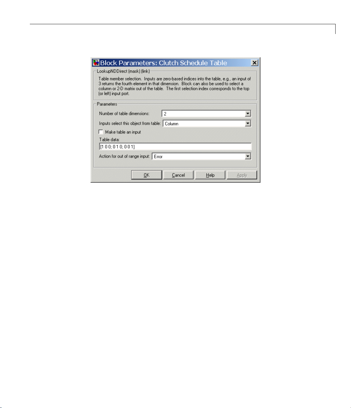
Combining Clutches and Gears into Transmissions

Thetableisindexed,startingfromzero, in both row and column. An input signal of 0 causes the block to output the first column of table values; a value of 1 outputs the second column; and a value of 2, the third column. The first column applies zero pressure to the two gear clutches and enables the Brake Switch in the main model. Turning this switch on applies full pressure to the brake clutch. Turning it off releases the brake pressure. The second column applies full pressure to the low gear clutch and zero pressure to the high gear and the brake clutches. The third column applies full pressure to the high gear clutch and zero pressure to the other two.

These different table columns are activated by changing the positions of the two M anual Switch b locks, labeled G ea r Switch and Neutral Switch. Putting the transmission into “neutral” and enabling the brake (upper position of Neutral Switch) feeds a zero signal to Clutch Schedule Table and activates the braking schedule. Switching the brake to off (lower position) allows the Gear Switch schedule signal to pass through instead. This signal has value 1 forthelowgearand2forthehighgear.

This clutch control subsystem is adequate for a simple model like this one, but not realistic. A full clutch control model requires realistic clutch pressure signals that rise from and fall back to zero in a smooth way. See “Shaping

2-47

2 Simple Models

Realistic Clutch Pressure Signals” on page 2-57 for more about modeling realistic clutch control pressures.

Running the Model, Switching Gears, and Braking

To see how gear switching works,

1 Start the model.

Its initial transmission state is low gear. The driven shaft spins at one-fifth therateofthedrivershaft.

2 Change the Gear Switch from Low to High, and observe how the driven

shaft velocity increases in the Shaft Velocities scope.

The driven-to-driver ratio is no w one-half. (The driver shaft velocity decreases slightly, because it experiences the damping torque on the driven shaft differently depending on which gear is engaged.)

3 Change the Gear Switch back to Low, then observe that the driven shaft

again spins more slowly.

2-48

At the same tim e, while you switch the gears back and forth, the clutches, asshownintheClutchModesscope,switchfromLoGearClutchbeing locked, to the Hi Gear Clutch being locked, and back. When one is locked, the other is unlocked.

4 Now enable the brake by changing the Neutral Switch to the upper position.

The two gear clutches unlock and dis engage . The driven shaft, subject to very light damping, now slows gradually. The Brake Clutch remains unengaged.

5 By turning the Brake Switch to on, you can switch the Brake Clutch to the

locked mode and bring the driven shaft to an immediate and complete stop. The driver shaft continues to spin at 10 radians/second.

Running the Model Without Clutch Mode Iteration

In realistic transmissions, the pressure signal applied to one clutch is often determined by the locked/unlocked mode of another clutch. Simulation of such a system requires simulation timetobrieflystopprogressingandmode

Combining Clutches and Gears into Transmissions

iteration to search for a self-consistent state of all clutches across the entire driveline.

This transmission is simple and non-self-referential, insofar as each clutch is controlled by external signals only. No clutch is controlled by the mode of another clutch. In such a case, you do not need mode iteration for the clutches, because the simulation does not have to search for a collective self-consistent state of all clutches. The externally imposed clutch schedule does that automatically.

To turn off clutch mode iteration,

1 Open the model’s Driveline Environment block (the block with the “Env”

icon).

2 Select the Disable m od e iteration for clutch locking check box.

3 Start the model again. The model runs faster and without mode iterations.

Disabling clutch mode iteration to avoid algebraic loops is sometimes necessary when you are using code generation-based simulation options in Simulink and Real-Time Workshop. See the Controllable Friction Clutch and Driveline Environment block reference pages for more details.

Adding Realistic Clutch Signals

The most critical addition you can make to the drive_strans_ideal model for greater realism is to change the clutch pressure signals from step functions (0 to 1, or 1 to 0) to signals with a smooth rise and fall. A variant model, drive_strans, has smoothed clutch pressure signals. The price of this greater realism is a potentially more complex model. It is critical for Simulink to determine transmission motion for exactly two clutches to always remain locked, or for all four to be unlocked, at any instant. Changing the transmission’s gear settings while maintaining this requirement is an example of the central problem of transmission design.

The final case study of the chapter, “Modeling and Simulating a Complete Car” on page 2-58, implements smoothed clutch pressure signals. See “Shaping Clutch Pressure Signals” on page 2-69.

2-49

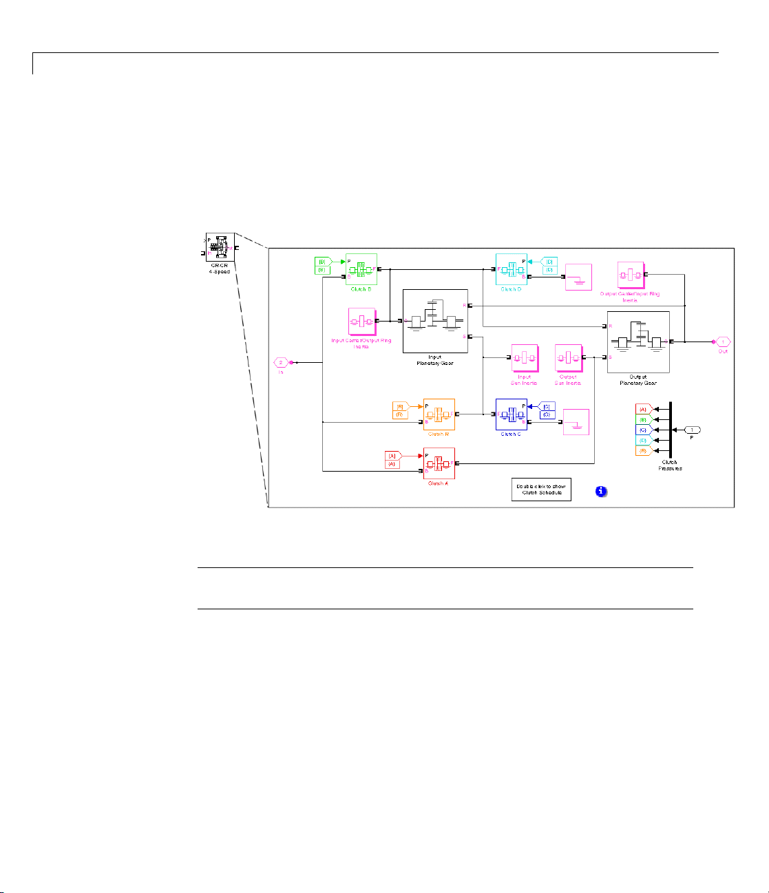
2 Simple Models

Introducing the

The SimDrivelin complete, worki library are unm subsystem open

CR-CR 4-Speed Transmission Template Subsystem

e Transmission Templates library provides examples of ng multiclutch transmission subsystems. The blocks in this asked. If you copy one into a model and double-click it, the s directly, allowing you to inspect the component blocks.

Transmission Templates Library

2-50

Note The Transmission blocks are not library-linked. Once you make a copy from the library to your model, you are free to modify your copy.

Each type of transmission block has its own clutch schedule, which you can view by opening the subsystem, then opening the clutch schedule block inside. (The corresponding block reference pages also list the clutch schedules for each Transmission block.) Properly engaging a transmission in a particular gear setting requires engaging a certain number of clutches, no more and no fewer. Locking too few or too many clutches, or engaging the wrong clutches, will lead to conflicting gear meshings and simulation errors. You can disen gage a transmission by setting all clutch pressure signals to 0.

Combining Clutches and Gears into Transmissions

Customizing and Using Transmission Blocks

Becauseyoudonothavetotakeanyextra steps to unlink a transmission block from its library, you can easily modify the Transmission block copies in your models. You will typical ly need to change gear ratios, clutch pressures, and gear shaft inertias in any case. If you open the Transmission block to view the underlying subsystem, you can proceed to modify blocks at will.

Caution Observe certain cautions when modifying the transmission subsystem component blocks:

• Do not rem ov e any of the gear shaft inertiablocksorsettheirinertiavalues

to 0. These inertias are needed for realistic simulation and preventing acceleration singularities when torques are applied.

• The clutch schedule for any transmission type specifies those clutches

that must be engaged and those that must be free at any instant for the transmission to be properly in gear. Make sure that your clutch pressures respect this requirement. Set all clutch pressures to 0 only if you want to disengage the transmission completely (place it in neutral). Do not engage any more or fewer clutches than needed, at any time during simulation.

• If you want to redesign the transmis s ion, by adding or removing gears,

you must consider whether you need as well to add or remove clutches and redesign the clutch schedule. You also might need to add or remov e gear shaft inertias.

The next section presents a driveline model based on the CR-CR 4-speed transmission model of the Transmissions library.

Modeling a CR-CR 4-Speed Transmission Driveline with Braking

The drive_crcr_ideal demo model builds on the previous clutch and transmission models with a more realistic transmission. (This is the same model presented in “Running a Demo Model” on page 1-6.) It uses the CR-CR 4-Speed transmission block from the Transmissions library to transfer motion

2-51

2 Simple Models

and torque from one shaft and inertia to another. T he model is otherwise similar to drive_strans_ideal.

CR-CR 4-Speed Transmission Model

2-52

A Torque Driver subsystem feeds a constant driving torque to the driver shaft (Inertia1). Two damping subsystems apply hea vy and light kinetic friction to the driver and driven shafts, respectively. The three Scopes measure the shaft velocities, clutch pressures, and clutch modes, respectively. T he model pre-load function defines essential parameters in the workspace. You can view these by opening the Workspace Variables block or opening the Callbacks tab of the File > Model Properties dialog. The CR-CR 4-Speed transmission subsystem couples the driver to the driven shaft (Inertia2). A brake clutch and fixed housing allow you to brake the driven shaft if the transmission is disengaged. When you first open the model, the Clutch Control subsystem contains a set of program med clutch signals for shifting the CR-CR transmission through a preconfigured gear and braking sequence over 30 seconds.

For clarity, the model’s major signal buses have been bundled as vectors and directed using Goto and From blocks. The Scopes are collected in the Scopes subsystem for convenience.

lacing Programmed with Controllable Clutch Pressures

Rep

To achieve manual control over the clutch pressure s,

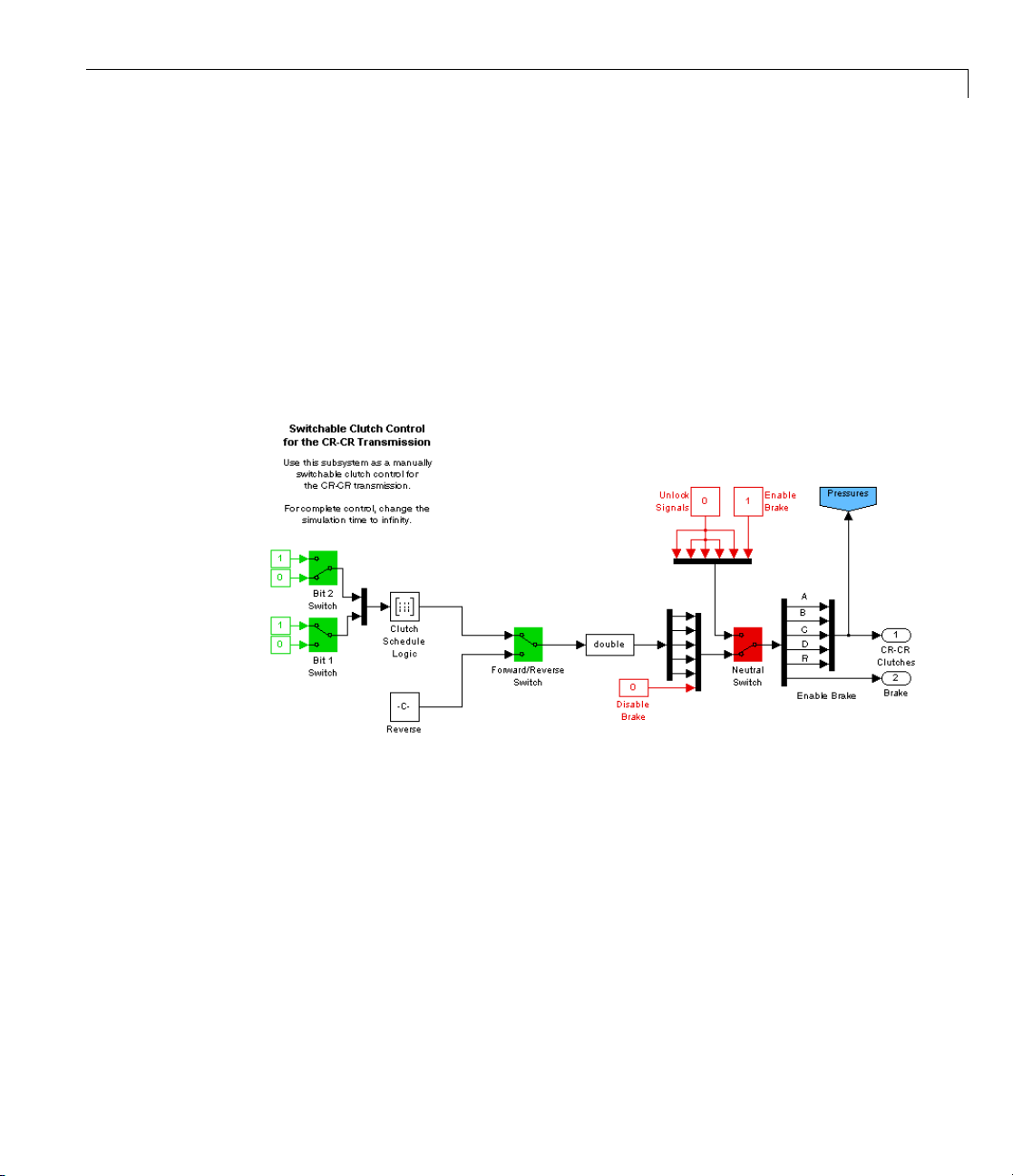
Combining Clutches and Gears into Transmissions

1 Change the sim ulation time in the Simulink model to o lbar from 30 to inf.

2 Open the drive_crcr_clutch_control_switch model and convert the entire

model to a replacement Clutch Control subsystem. (This model is not intended to be run by itself.)

3 Delete the original Clutch Control subsystem in drive_crcr_ideal and

replace it with this new subsystem.

When you have completed these steps, you can run the model without stopping and manually switch the transmission into different gear settings.

Manual

Clutch Control for CR-CR Transmission

Configuring the CR-CR Transmission Subsystem

R-CR 4-Speed transmission block used in drive_crcr_ideal has

The C

ult settings for its component Gears, Clutches, and Inertias, with some

defa

ptions. C ertain parameters are changed for greater realism and are

exce

renced to variables defined in the workspace when the model opens. These

refe

iables are used in the four CR-CR Clutch blocks A, B, C, and D. (Ignore

var

reverse gear clutch, Clutch R.)

the

2-53

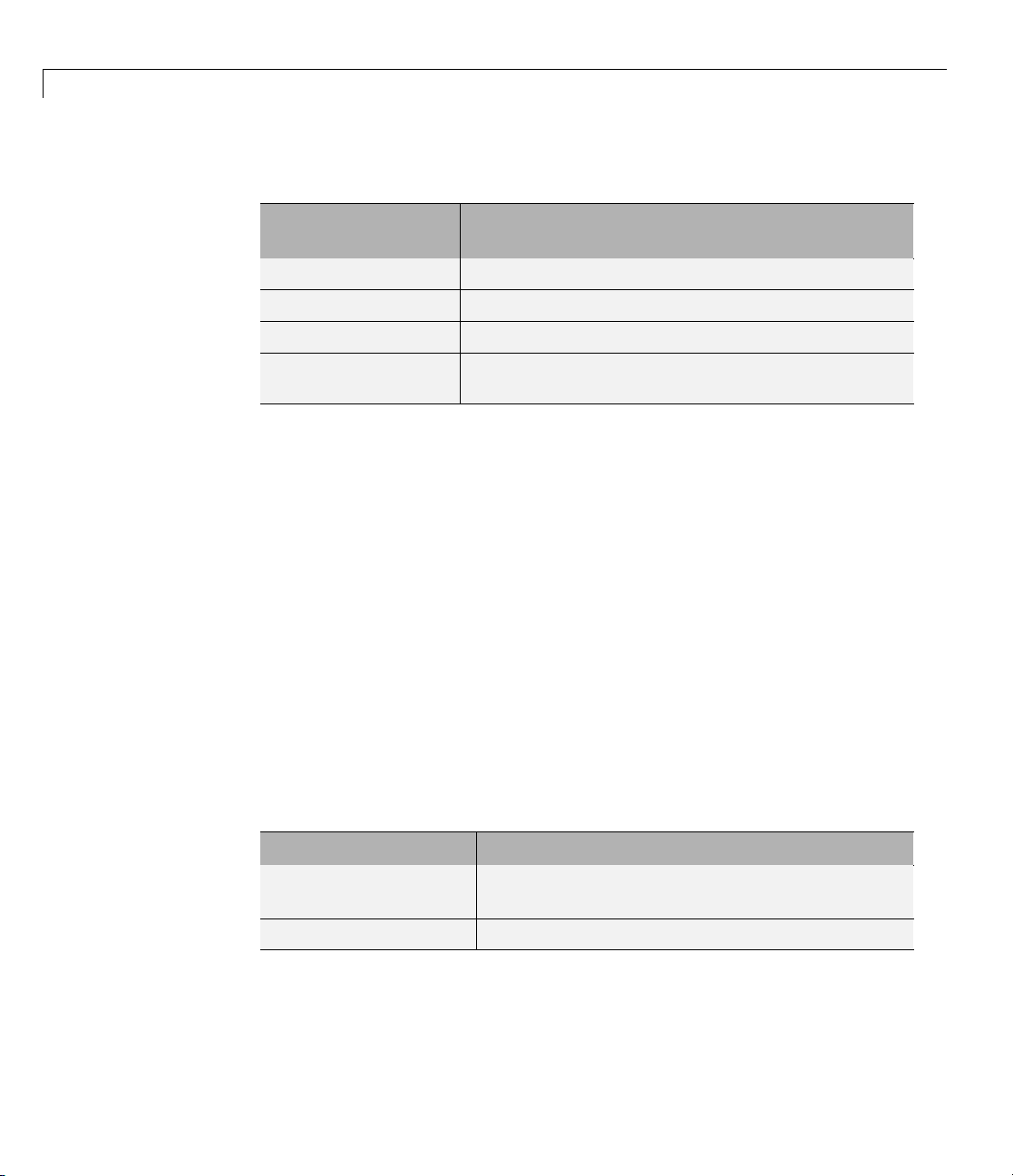
2 Simple Models

CR-CR 4-Speed Transmission Clutch Variables

Workspace

Meaning

Variable

num_fric_surf

eff_tor_rad

peak_normal

fric_coeff (matrix) Kinetic friction coefficient as a function of the

Number of frictional surfaces in each clutch

Effective torque radius in each clutch (m)

Peak normal force on clutch surfaces (N)

relative angular velocity of the clutch shafts

Within the CR-CR transmission subsystem,

1 Open the Clutch Schedule block to see the table of gear settings, clutch

lockings, and gear ratios. (The CR–CR 4-Speed block reference page also discusses the clutch schedule.)

There are four distinct (forward) gear settings, each with a different effective gear ratio. For the transmission to be properly engaged and transmit torque and motion, exactly two clutches must be locked at any instant. Unlocking all the clutches simultaneously puts the transmission into neutral (no motion or torque transfer).

2 Close t

The mai dampi trans

he transmission subsystem and return to the main m odel window.

n model’s Damping subsystems use these variables for frictional

ng of the driving (engine) and driven shafts coupled across the

mission.

2-54

Drive

Shaft Damping Coefficients

Workspace Variable

eng_damping

driven_damping

Meaning

Driver (engine) shaft kinetic friction coefficient (N·m·s/rad)

Driven shaft kinetic friction coefficient (N·m·s/rad)

Combining Clutches and Gears into Transmissions

Programming the Clutch Schedule Logic

Note This and the following sections assume you have replaced the original

programmed Clutch Control subsystem with the manually switchable replacement subsystem. See “Replacing Programmed with Controllable Clutch Pressures” on page 2-52.

From the main model, open the Clutch Control subsystem. The Clutch Schedule Logic block embo dies the CR-CR 4-Speed clutch schedule as a truth table for the four forward gears. Each row re presents a different gear setting. You select a particular row for output by inputting a set of 1’s and 0’s that specify the row value as a binary number.

CR-CR 4-Speed Clutch Schedule Log ic

Gear Setting

201

310

Truth Table Row Truth Table Value

=0 10010

=1 10100

=2 11000

=3 01100

In the order of the CR-CR Clutches — A, B, C, and D, respectively — the sequence of 1’s and 0’s indicates which clutches are locked (1) and which are free (0). These Boolean values are then converted into normalized clutch pressure signals. The fifth value in each row represents the disengaged reverse gear Clutch R.

Programming the Reverse Gear. By default, the Forward/Reverse Switch is set to the up position, placing the transmissioninforwardmotion. Ifyou want to engage the reverse gear, flip the switch to the down position.

Open the corresponding Reverse block to see the reverse gear clutch schedule as a truth table.

2-55

2 Simple Models

CR-CR Reverse Gear Clutch Schedule Logic

Gear Setting

Reverse

Truth Table Value

00011

Running the CR-CR Transmission Model — Changing Gears

You are now ready to run the model.

1 Open the Scopes subsystem, then the individual Scope blocks. Close the

Scopes subsystem.

With the Scopes, you can observe the angular velocities of the driving and driven shafts, and the pressures and modes of the four clutches.

2 Open the Clutch Control subsystem. (This should be the manually

switchable subsystem.) Ensure that the Forward/Reverse Switch is set to up and the Neutral Switch to down.

Start the model. You can change the forward gear settings by flipping the Bit0 and Bit1 Switch b locks and moving through truth table entries corresponding to each setting. (See the table, CR-CR 4-Speed Clutch Schedule Logic on page 2-55.) Switching from one gear setting to another unlocks some clutches and locks others, but always leaves two clutches locked. As you flip betwee n gear settings, the transmission transfers motion and torque at different ratios.

2-56

3 You can disengage the CR-CR transmission completely by flipping the

Neutral Switch to up. This step also enables the Brake Switch in the main model. (If the transmission is engaged, not in neutral, the Brake Switch is disabled.)

If the transmission is disengaged but without braking, the driven shaft velocity slowly decreases under the influence of frictional damping. If you brake, however, by switching on the Brake Switch, the driven shaft velocity im mediately drops to 0. Th e braking here works the same way as in the p revious examples.

Combining Clutches and Gears into Transmissions

4 You can put the CR-CR transmission into reverse by keeping the Neutral

Switch flipped to down and by flipping the Forward/Reve rse Switch to down.

As with a real transmission, it is best to transition the transmission model through neutral and bring the driven shaft to a rest before putting the transmission into reverse gear.

Shaping Realistic Clutch Pressure Signals

The drive_crcr_ideal model allows you to switch forward gear settings without placing the CR-CR transmission in neutral. Of course, controlling a real manual transmission requires moving the transmission out of gear and into neutral, picking a new gear setting, then putting the transmission into the new gear. You can mimic these steps by flipping the Neutral Switch on, changing the gear setting, then slipping the Neutral Switch off.

The most critical addition you can make to this model for greater realism is to change the clutch pressure signals from step functions (0 to 1, or 1 to 0) to signals with a smooth rise and fall. A variant model, drive_crcr, has smoothed clutch pressure signals. The price of this greater realism is a potentially more complex model. It is critical for Simulink to determine transmission motion for exactly two clutches to always remain locked, or for all four to be unlocked, at any instant. Changing the CR-CR transmission’s gear settings while maintaining this requirement is an example of the central problem of transmission design.

The following case study, “Modeling and Simulating a Complete Car” on page 2-58, implements smoothed clutch pressure signals. See “Shaping Clutch Pressure Signals” o n page 2-69.

2-57

2 Simple Models

Modeling and Simulating a Complete Car

In this section...

“About the Full Car Model” on page 2-58

“Modeling the Engine” on page 2-59

“Modeling the Transmission” on page 2-61

“Coupling the Engine to the Transmission” on page 2 -62

“Modeling the Wheel Assembly and Road Coupling” on page 2-63

“Controlling the Clutches and Braking” on page 2-67

“Running the Model” on page 2-70

About the Full Car Model

The full car drivetrain simulation of the drive_full_car demo encompasses all the points of this chapter and many key SimDriveline features. It includes engine and transmission models and a simplified model of the drivetrain-wheel-road coupling. The engine and transmission are coupled with a torque converter. Programmed clutch control steps the transmission through four gears and neutral before a braking torque is applied. The clutch press ure signals are smooth and more realistic than the sharp clutch pressure signals used in the preceding studies. This section explains these features, subsystems, and their relationship and purposes, leading you to actual simulation.

2-58

Understanding the Model’s Global Structure

Open the demo. The model pre-load function defines a set of workspace variables in MATLAB used by some of the blocks. N ote the major systems of this car model.

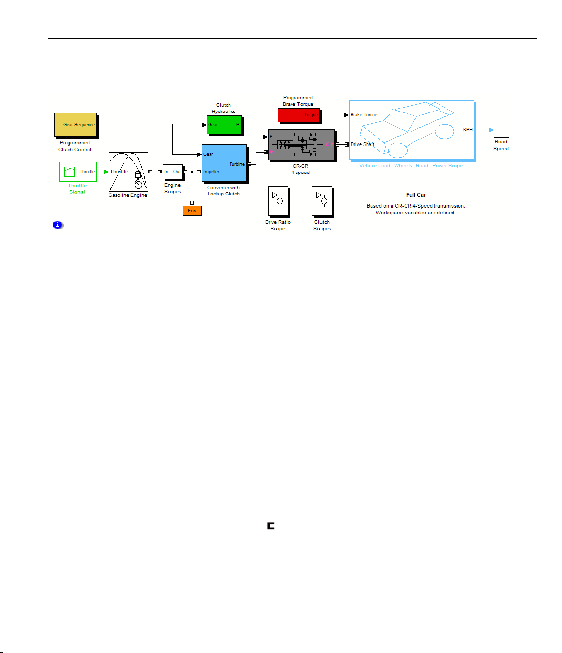
Full Car Model

Modeling and Simulating a Complete Car

The main driveline subsystems are

• Engine

• Torque converter

• Transmission

The large subsystem to the right represents the final part of the drivetrain: the vehicle inertia, the wheels, their coupling to the road, and braking. All the other subsystems in the model represent inputs that control the drivetrain or outputs that measure its behavior.

Modeling the Engine

SimDriveline software is primarily devoted to modeling the rotational dynamics of drivelines, accepting rotational power from any source that can be modeled in Simulink and converted to a connection line transferring torque. In most applications, your modeled driveline power and torque sources will represent engines and motors. For the purposes of system modeling, an engine or motor specifies an output torque as a function of driveline speed. However you specify the behavior of theengineormotor,itsSimDriveline output is a connector port

transferring torque to the rest of the system.

2-59

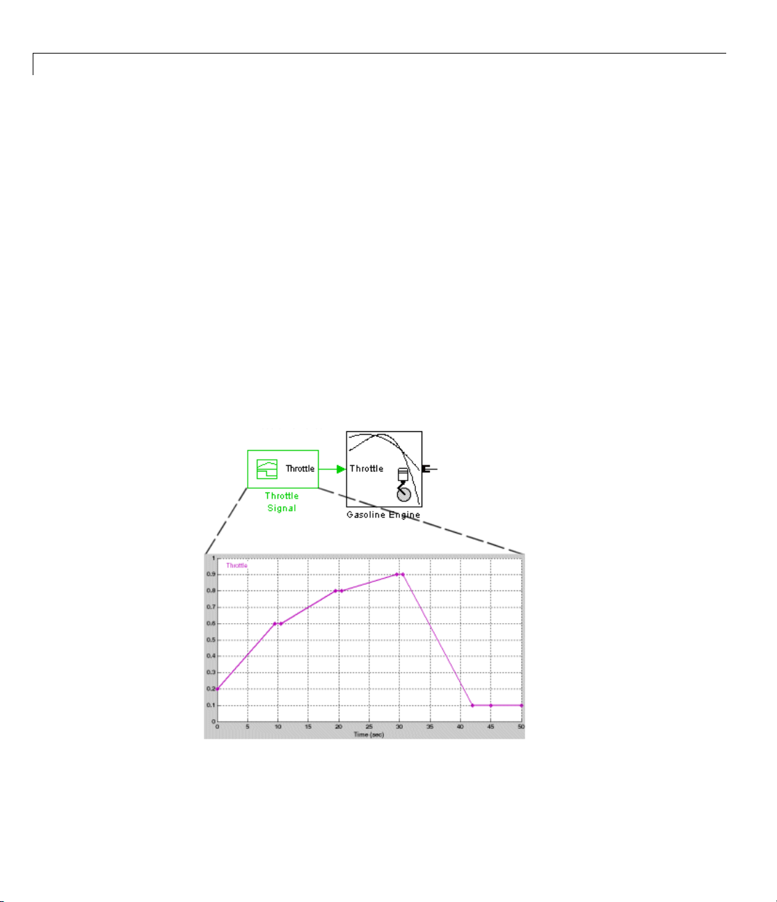
2 Simple Models

Using an Engine Block from Vehicle Components

The Vehicle Components library containsblocksrepresentingsimpleengine models. You control these engine models with a Simulink throttle signal. The heart o f the engine model is a function that specifies the maximum engine torque possible for each engine speed. The throttle signal controls how much torque, out of this maximum possible, the engine can deliver. The m aximum possible torque itself is a function of the engine speed at any instant.

The drive_full_car demo uses a Gasoline Engine block from Vehicle Components. Th e block’s properties specified i n its dia log inclu d e the engi n e’s maximum power, its speed at maximum power, and its maximum possible speed. The throttle signal is programmed by a Signal Builder block that specifies a time-depend throttle profile over the course of the simulation. Open these block dialogs to view these settings and the throttle profile. The throttle signal is programmed to produce a realistic acceleration profile and to be consistent with the gear shifting sequence discussed in “Controlling the Clutches and Braking” on page 2-67.

2-60

Engine Throttle Signal Profile

Modeling and Simulating a Complete Car

Learn more about the Engine block models from their b lock reference pages. See also “Vehicle Components” on page 2-5.

Alternative and Advanced Methods for Modeling Engines

The engine models of the Vehicle Components library are simple. You can create your own, more complex, engine models by elaborating on the b asic pattern of engine speed determining enginetorqueoutput. Thecomplete engine model involves a feedback loop because the output torque, once connected to the external load, determines how fast the output driveshaft spins. The engine model then uses this output speed to set the maximum possible torque.

Several important engine features to consider in a more complete model would be

• Distinguishing steady-state behavior from engine start-up, when the

engine speed-engine torque function has not yet reached its maximum possible envelope

• Details of mechanical power production, such as air-fuel compression and

combustion, or electromagnetic induction

• Additional controls beyond what can be represented by a single throttle

signal

Modeling the Transmission

The CR-CR 4-speed transmission subsystem in the drive_full_car model is similar to the previous example, “Modeling a CR-CR 4-Speed Transmission Driveline with Braking” on page 2-51. The clutch and planetary gear properties are set in the block dialogs with workspace variables.

Workspace Variable

inPlanetRatio

outPlanetRatio

numFricSurf

effTorqueRadius

Meaning

Gear: input planetary gear ring/sun ratio

Gear: output planetary gear ring/sun ratio

Clutch: number of surface friction surfaces

Clutch: effective torque radius (m)

2-61

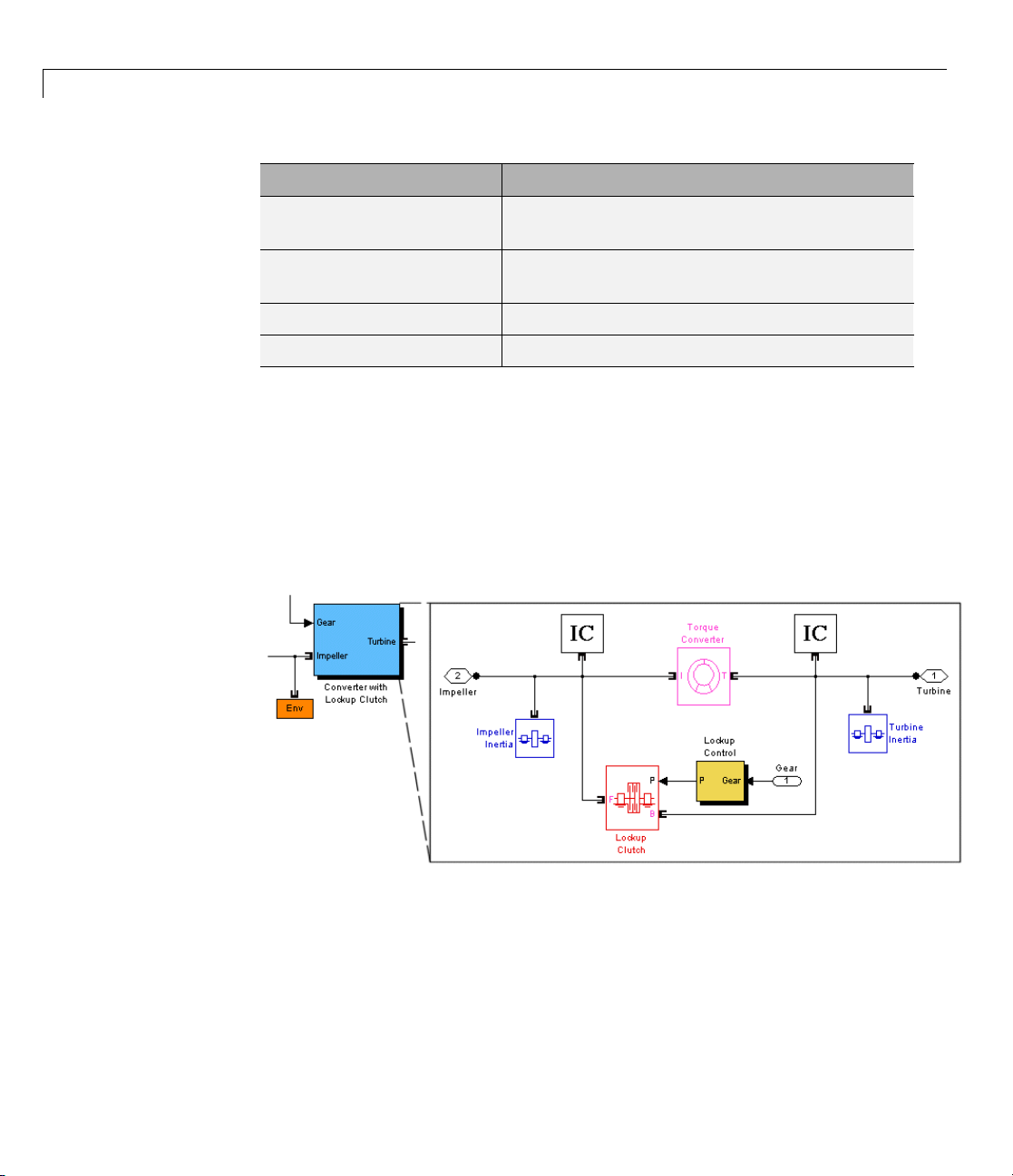
2 Simple Models

Workspace Variable

peakNormForce

coeffFricTable (matrix) Clutch: surface friction function (tabulated

staticFricPeak

velTol

For more about gears, clutches, and transmissions, see the Controllable Friction Clutch and CR–CR 4-Speed block reference pages, as well as “Gears” on page 2-4 and “Transmission Templates” on page 2-5.

Meaning

Clutch: peak normal force on friction surfaces (N)

discrete function)

Clutch: static (locking) friction peak factor

Clutch: clutch velocity locking tolerance (rad/s)

Coupling the Engine to the Transmission

The drive_full_car model couples the engine and the transmission through a torque converter subsystem.

2-62

Torque Converter Subsystem

A torque converter, like a clutch, couples two independent driveline axes in such a way as to transfer angular motion and torque from an input to an output shaft. However, unlike a clutch, a torque converter never locks and the output shaft never exactly reaches the speed of the input. (The torque converter transfers motion by hydrodynamic viscosity, not by surface friction.)

Modeling and Simulating a Complete Car

So a torque converter does not step through discrete stages and avoids the motion discontinuities inherent in friction clutches.

To mimic engine idling at the start of the simulation, the initial condition (IC) actuators start the input and output shafts at nonzero velocities.

The clutch in this subsystem is present to lock the input and output shafts together once the main clutches of the transmission have reached the highest gear. See “Controlling the Clutches and Braking” on page 2-67.

See the To rque Converter and Initial Condition block reference pages for more details about these blocks.

Modeling the Wheel Assembly and Road Coupling

The CR-CR 4-speed transmission feeds its output torque to the final drive subsystem, Vehicle Load - Wheels - Road - Power Scope, which represents the vehicle inertia (the load on the transmission), the wheels, and the wheel contact with the road. This subsystem also incorporates a brake model that can impose, with the appropriate input signal, a brake torque on the wheels. This torque acts on the driveline in addition to the reaction stress imposed by the wheel contact with the road. The wheel-road load model is implemented with Simulink alone.

This final drive subsystem is masked. Open it by right-clicking it, then selecting Look Under Mask.

2-63

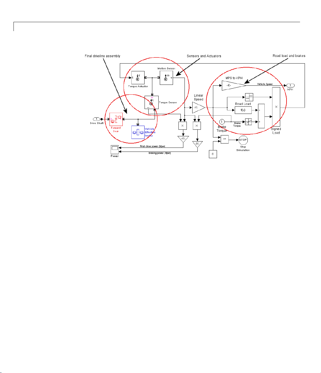
2 Simple Models

Final Drive Subsystem: Vehicle Load, Wheels, and Road Coupling

The subsystem has three major areas:

2-64

• Ontheleftmostpartofthediagramisthe terminus of the driveline proper,

where the driveline connection lines end.

• Attheupperleftareacollectionofsensor and actuator blocks coupling the

driveline proper to the wheels and brakes.

• In the center and right are the Simulink blocks that model the wheel-road

coupling and braking.

Modeling the Final Driveline Assembly and Vehicle Load

The driveline connection line sequence of the whole full car model ends with the first set of blocks on the left of the subsystem. The torque and motion are transferred forward through the Forward Gear and are loaded down with the Vehicle Effective Inertia. Two workspace variables specify the relevant variables.

Mathworks SIMDRIVELINE 1 user guide

Specifications and Main Features

Frequently Asked Questions

User Manual

Introducing SimDriveline Software

Product Overview

Product Definition

Driveline Simulation and Physical Modeling

Related Products

Required Products

Other Related Products

Physical Modeling Product Family

For Information About MathWorks Products

Running a Demo Model

What the Model Represents

What the Model Illustrates

Clutch Schedule for the CR-CR 4-Speed Transmission

Opening the Model

Opening General SimDriveline Demos

The Block Diagram Model

What the Model Contains — Opening the Subsystems

Modifying the Model

Measuring the Drive Ratio of the CR-CR Transmission States

What Can You Do with SimDriveline Software?

About SimDriveline Software

Modeling Drivetrains

Connector Ports and Connection Lines

Inertias and Gears

Complex Driveline Elements

Actuating and Sensing Motion

Trimming and Linearizing the Motion

Generating Code — Clutches and Algebraic Loops

Learning More

Using the MATLAB Help System for Documentation and Demos

Finding Special SimDriveline Help

Simple Models

Introducing the SimDriveline Block Libraries

About the SimDriveline Block Library

Accessing the Libraries

SimDriveline Library

Using the Libraries

Solver & Inertias

Gears

Dynamic Elements

Transmission Templates

Sensors & Actuators

Interface Elements

Vehicle Components

Essential Steps to Building a Driveline Model

Representing and Transferring Driveline Motion and Torque

About Inertia, Motion, and Gears

Coupling Rotational Motion with Gears

Gear Coupling Rules

Generalized Gear Coupling Rules

Modeling Two Spinning Inertias

Coupling Two Spinning Inertias with a Simple Gear

Torque-Actuating Two Coupled, Spinning Inertias

Sensing and Actuating Motion and Torque

Coupling Two Spinning Inertias with a Variable Gear

Coupling Three Spinning Inertias with a Planetary Gear

Actuating Drivelines with Torques and Motions

About Torques, Motions, and Actuation

Stabilizing Numerical Derivatives in Actuator Signals

Actuating a Driveline with Torques

Actuating a Driveline with Motions

Setting the Motion Initial Conditions of a Driveline

Resolving Undetermined Motions in Complex Gears

Controlling Gear Couplings with Clutches

About Motion, Gears, and Clutches

Engaging and Disengaging Gears with Clutches

How a Clutch Works

Engaging and Disengaging a Gear with a Clutch

Modeling Realistic Clutch Systems with Loss

Creating a Torque Damping Subsystem

Connecting and Simulating the Damped Clutch S ystem

Braking Motion with Clutches

Braking with a Double-Clutch System

Combining Clutches and Gears into Transmissions

About Gears, Clutches, and Transmissions

Modeling a Simple Two-Speed Transmission with Braking