Mathworks SIGNAL PROCESSING BLOCKSET 7 user guide

Download

Signal Processing

User’s Guide

Blockset™ 7

How to Contact The MathWorks

www.mathworks. comp.soft-sys.matlab Newsgroup www.mathworks.com/contact_TS.html T echnical Support

suggest@mathworks.com Product enhancement suggestions

bugs@mathwo doc@mathworks.com Documentation error reports service@mathworks.com Order status, license renewals, passcodes

info@mathwo

com

rks.com

Web

Bug reports

Sales, prici

ng, and general information

508-647-7000 (Phone)

508-647-7001 (Fax)

The MathWorks, Inc. 3 Apple Hill Drive Natick, MA 01760-2098

For contact information about worldwide offices, see the MathWorks Web site.

Signal Processing Blockset™ User’s Guide

The software described in this document is furnished under a license agreement. The software may be used or copied only under the terms of the license agreement. No part of this manual may be photocopied or reproduced in any form without prior written consent from The MathW orks, Inc.

FEDERAL ACQUISITION: This provision applies to all acquisitions of the Program and Documentation by, for, or through the federal government of the United States. By accepting delivery of the Program or Documentation, the government hereby agrees that this s oftware or docume n tation qualifies as commercial computer software or commercial computer software documentation as such terms are used or defined in FAR 12.212, DFARS Part 227.72, and DFARS 252.227-7014. Accordingly, the terms and conditions of this Agreement and only those rights specified in this Agreement, shall pertain to and govern theuse,modification,reproduction,release,performance,display,anddisclosureoftheProgramand Documentation by the federal government (or other entity acquiring for or through the federal government) and shall supersede any conflicting contractual terms or conditions. If this License fails to meet the government’s needs or is inconsistent in any respect with federal procurement law, the government agrees to return the Program and Docu mentation, unused, to The MathWorks, Inc.

Trademarks

MATLAB and Simulink are registered trademarks of The MathWorks, Inc. See

www.mathworks.com/trademarks for a list of additional trademarks. Other product or brand

names may be trademarks or registered trademarks of their respective holders.

Patents

The MathWorks products are protected by one or more U.S. patents. Please see

www.mathworks.com/patents for more information.

Revision History

April 1995 First printing New for Version 1.0 May 1997 Second printing Revised for Version 2.0 January 1998 Third printing Revised for Version 2.2 (Release 10) January 1999 Fourth printing Revised for Version 3.0 (Release 11) November 2000 Fifth printing Revised for Version 4.0 (Release 12) June 2001 Online only Revised for Version 4.1 (Release 12.1) July 2002 Sixth printing Revised for Version 5.0 (Release 13) April 2003 Seventh printing Revised for Version 5.1 (Release 13SP1) June 2004 Online only Revised for Version 6.0 (Release 14) (Renamed from DSP

Blockset User’s G uide) October 2004 Online only Revised for Version 6.0.1 (Release 14SP1) March 2005 Online only Revised for Version 6.1 (Release 14SP2) September 2005 Online only Revised for Version 6.2 (Release 14SP3) March 2006 Online only Revised for Version 6.3 (Release 2006a) September 2006 Online only Revised for Version 6.4 (Release 2006b) March 2007 Online only Revised for Version 6.5 (Release 2007a) September 2007 Online only Revised for Version 6.6 (Release 2007b) March 2008 Online only Revised for Version 6.7 (Release 2008a) October 2008 Online only Revised for Version 6.8 (Release 2008b) March 2009 Online only Revised for Version 6.9 (Release 2009a) September 2009 Online only Revised for Version 6.10 (Release 2009b) March 2010 Online only Revised for Version 7.0 (Release 2010a)

Working with Signals

Discrete-Time Signals .............................. 1-2

Time and Frequency Terminology Recommended Settings for D i screte-Time Simulations Other Settings for Discrete-Time Simulations

.................... 1-2

.......... 1-6

Contents

... 1-4

Continuous-Time Signals

Continuous-Time Source Blocks Continuous-Time Nonsource Blocks

Sample-Based Signals

Sample-Based Single Channel Signals Sample-Based Multichannel Signals

Frame-Based Signals

Frame-Based Single Channel Signals Frame-Based Multichannel Signals Benefits of Frame-Based Processing

Creating Sample-Based Signals

Using the Constant Block Using the Signal from Workspace Block

Creating Frame-Based Signals

Using the Sine Wave Block Using the Signal from Workspace Block

Creating Multichann el Sample-Based Signals

Multichannel Sample-Based Signals Combining Single-Channel Sample-Based Signals Combining Multichannel Sample-Based Signals

........................... 1-11

...................... 1-11

.................. 1-11

.............................. 1-13

................ 1-13

.................. 1-13

............................... 1-15

................. 1-15

................... 1-15

.................. 1-16

..................... 1-19

........................... 1-19

............... 1-21

...................... 1-25

.......................... 1-25

............... 1-28

.................. 1-32

........ 1-32

....... 1-32

........ 1-35

Creating Multichann el Frame-Based Signals

......... 1-38

Multichannel Frame-Based Signals ................... 1-38

Combining Frame-Based Signals

..................... 1-39

Deconstructing Multichannel Sample-Based Signals

Splitting Multichannel Sample-Based Signals into

Individual Signals

Splitting Multichannel Sample-Based Signals into Several

Multichannel Signals

Deconstructing Multichannel Frame-Based Signals

Splitting Multichannel Frame-Based Signals into

Individual Signals

Reordering Channels in Multichannel Frame-Based

Signals

Importing and Exporting Sample-Based Signals

Importing Sample-Based Vector Signals Importing Sample-Based Matrix Signals Exporting Sample-Based Signals

Importing and Exporting Frame-Based Signals

Importing Frame-Based Signals Exporting Frame-Based Signals

Displaying Time-Domain Data

Displaying Time Domain Data in the Vector Scope Displaying Time-Domain Data in the Time Scope

........................................ 1-54

............................... 1-42

............................ 1-45

............................... 1-49

...... 1-58

............... 1-58

.............. 1-61

..................... 1-65

....... 1-70

..................... 1-70

..................... 1-73

...................... 1-79

...... 1-79

....... 1-82

.. 1-42

... 1-49

vi Contents

Displaying Frequency-Domain Data

................. 1-100

Advanced Signal Concepts

Inspecting Sample Rates and Frame Rates ........... 2-2

Sample Rate and Frame Rate Concepts Inspecting Sample-Based Signals Using the Probe Block Inspecting Frame-Based Signals Using the Probe Block Inspecting Sample-Based Signals Using Color Coding

............... 2-2

.. 2-3 .. 2-5

.... 2-7

Inspecting Frame-Based Signals Using Color Coding .... 2-9

Converting Sample and F ram e Rates

Rate Co nv ersion Blocks Rate Conversion by Frame-Rate Adjustment Rate Conversion by Frame-Size Adjustment Avoiding Unintended Rate Conversion Frame Rebuffering Blocks Buffering with Preservation of the Signal Buffering with Alteration of the Signal

Converting Frame Status

Frame Status Buffering Sample-Based Signals into Frame-Based

Signals

Buffering Sample-Based Signals i nto Frame-Based Signals

with Overlap

Buffering Frame-Based Signals into Other Frame-Based

Signals Buffering Delay and Initial Conditions Unbuffering Frame-Based Signals into Sample-Based

Signals

Delay and Latency

Computational Delay Algorithmic Delay Zero Algorithmic Delay Basic Algorithmic Delay Excess Algorithmic Delay (Tasking Latency) Predicting Tasking Latency

..................................... 2-33

........................................ 2-33

................................... 2-37

........................................ 2-41

........................................ 2-45

............................ 2-11

.......................... 2-24

........................... 2-33

................................. 2-49

.............................. 2-49

................................. 2-51

............................. 2-51

............................ 2-54

......................... 2-59

................ 2-11

........... 2-12

............ 2-15

................ 2-19

.............. 2-27

................ 2-30

................ 2-44

........... 2-57

Digital Filter Block ................................ 3-2

Overview o f the Digital Filter Block Implementing a Lowpass Filter Implementing a Highpass Filter Filtering High-Frequency Noise

.................. 3-2

...................... 3-3

..................... 3-4

...................... 3-5

Filters

vii

Specifying Static Filters ............................ 3-9

Specifying Time-Varying Filters Specifying the SOS Matrix (Biquadratic Filter

Coefficients)

.................................... 3-15

..................... 3-10

Digital Filter Design Block

Overview o f the Digital Filter Design Block Choosing Betw een Filter Design Blocks Creating a Lowpass Filter Creating a Highpass Filter Filtering High-Frequency Noise

Filter Realization Wizard

Overview o f the Filter Realization Wizard Designing and Implementing a Fixed-Point Filter Setting the Filter Structure and Number of Filter

Sections

Optimizing the Filter Structure

Analog Filter Design Block

Adaptive Filters

Creating an Acoustic Environment Creating an Adaptive Filter Customizing an Adaptive Filter Adaptive Filtering Demos

Multirate Filters

Filter Banks Multirate Filtering Examples

....................................... 3-48

................................... 3-53

................................... 3-66

...................................... 3-66

......................... 3-17

............... 3-18

.......................... 3-21

.......................... 3-23

...................... 3-25

........................... 3-31

............. 3-31

...................... 3-49

......................... 3-51

................... 3-53

......................... 3-55

...................... 3-60

........................... 3-64

........................ 3-74

............ 3-17

....... 3-32

viii Contents

Transforming Time-Domain Data into the Frequency

Domain

......................................... 4-2

Transforms

Transforming Frequency-Domain Data into the Time

Domain

......................................... 4-7

Linear and Bit-Reversed Output Order

FFT and IFFT Blocks Data Order Finding the Bit-Reversed Order of Y our Frequency

Indices

Calculating the Channel Latencies Required for

Wavelet Reconstruction

Analyzing Your Model Calculating the Group Delay of Your Filters Reconstructing the Filter Bank System Equalizing the Delay on Each Filter Path Updating and Running the Model References

........................................ 4-12

.......................... 4-14

.............................. 4-14

....................................... 4-22

.................... 4-12

.................... 4-21

.............. 4-12

............ 4-16

................ 4-18

.............. 4-18

Quantizers

Scalar Quantizers ................................. 5-2

Analysis and Synthesis of Speech Identifying Your Residual Signal and Reflection

Coefficients

Creating a Scalar Quantizer

.................................... 5-4

.................... 5-2

......................... 5-5

Vector Quantizers

Building Your Vector Quantizer Model Configuring and Running Your Model

................................. 5-10

................ 5-10

................. 5-11

Statistics, Estimation, and Linear Algebra

Statistics .......................................... 6-2

Statistics Blocks

.................................. 6-2

Basic Operations .................................. 6-3

Running Operations

............................... 6-4

Power Spectrum Estimation

Linear Algebra

Linear Algebra Blocks Linear System Solvers Matrix Factorizations Matrix Inverses

.................................... 6-7

.............................. 6-7

.............................. 6-9

................................... 6-11

........................ 6-6

............................. 6-7

Working with Fixed-Point Data

Fixed-Point Signal Processing Development ......... 7-2

Fixed-Point Features Benefits of Fixed-Point Hardware Benefits of Fixed-Point Design with Signal Processing

Blockset Software

Fixed-Point Signal Processing Applications

Concepts and Terminology

Fixed-Point Data Types Scaling Precision and Range

.......................................... 7-6

.............................. 7-2

.................... 7-2

............................... 7-3

............ 7-4

......................... 7-5

............................ 7-5

............................... 7-7

x Contents

Arithmetic Operations

Modulo Arithmetic Two’s Complement Addition and Subtraction Multiplication Casts

Specifying Fixed-Point Attributes

Fixed-Point Block Parameters Specifying System-Level Settings Inherit via Internal Rule

........................................... 7-17

.................................... 7-14

............................. 7-11

................................ 7-11

................................ 7-12

........................... 7-13

....................... 7-22

........................... 7-26

................... 7-22

.................... 7-25

Example: Selecting and Specifying Data Types for

Fixed-Point Blocks

.............................. 7-37

Fixed-Point Filtering

Fixed-Point Filtering Blocks Filter Implementation Blocks Filter Design and Implementation Blocks

.............................. 7-45

......................... 7-45

........................ 7-45

.............. 7-46

Getting Started with System Objects

What Are System Objects? .......................... 8-2

Setting Up and Running System Objects

Creating an Instance of a System Object Using Methods to Run System Objects Finding Help and Demos for System Objects

Using System Objects with the Embedded MATLAB

Subset

Considerations for Using System Objects with the

Embedded MATLAB Subset Using System Objects with Embedded MATLAB Coder Using System Objects with the Embedded MATLAB

Function Block Using System Objects with Embedded MATLAB MEX

.......................................... 8-9

....................... 8-9

................................. 8-12

............. 8-3

............... 8-3

................ 8-6

........... 8-8

.. 8-11

... 8-12

Using Signal Processing System Objects

What Are Signal Processing System Objects? ......... 9-2

Generating Code for Signal Processing System

Objects

......................................... 9-3

Working with Signals and Fixed-Point Data .......... 9-5

What Are Sample- and Frame-Based Processing? Working with Fixed-Point Data

Example: Using System Objects in Signal Processing

Applications: Filtering an Audio Stream

...................... 9-10

....... 9-5

........... 9-15

Index

xii Contents

Working with Signals

This chapter helps you understand how sample-based and frame-based signals are represented in the Simulink single-channel and multichannel sample-based and frame-based signals. You also learn how to extract single-chan n el signals from multichannel signals. Lastly you explore how to import signals into signal processing models and export signals to the MATLAB

• “Discrete-Time Signals” on page 1-2

• “Continuous-Time Signals” on page 1-11

• “Sample-Based Signals” on page 1-13

• “Frame-Based Signals” on page 1-15

• “Creating Sample-Based Signals” on page 1-19

• “Creating Frame-Based Signals” on page 1-25

• “Creating Multichannel Sample-Based Signals” on page 1-32

• “Creating Multichannel Frame-Based Signals” on page 1-38

• “Deconstructing Multichannel Sample-Based Signals” on page 1-42

• “Deconstructing Multichannel Frame-Based Signals” on page 1-49

• “Importing and Exporting Sample-Based Signals” on page 1-58

• “Importing and Exporting Frame-Based Signals” on page 1-70

environment. You learn how to create

workspace.

• “Displayin g Time-Doma in Data” on page 1-79

• “Displaying Frequency-Domain Data” on pa g e 1-100

1 Working with Signals

Discrete-Time Signals

In this section...

“Time and Frequency Terminology” on page 1-2

“Recommended Settings for Discrete-Time Simulations” on page 1-4

“Other Settings for Discrete-Time Simulations” on page 1-6

Time and Frequency Terminology

Simulink models can process both discrete-time and continuous-time signals. Models built with Signal Processing Blockset™ software are often intended to process discrete-time signals only. A discrete-time signal is a sequence of values that correspond to particular instants in time. The time instants at which the signal is defined are the si gn al’s sample times, and the associated signal values are the signal’s samples. Traditionally, a discrete-time signal is considered to be undefined at points in time between the sample times. For a periodically sampled signal, the equal interval between any pair of consecutive sample times is the signal’s sample period, T

, is the reciprocal of the sample period, or 1/Ts. T h e sample rate is the

number of samples in the signal per second.

.Thesample rate,

1-2

The 7.5-second triangle wave segment below has a sample period of 0.5 second, and sam pl e times of 0.0, 0.5, 1.0, 1.5, ...,7.5. Th e sample rate of the sequence is therefore 1/0.5, or 2 Hz.

A number of different terms are used to describe the characteristics of discrete-time signals found in Simulink models. These terms, which are listed inthefollowingtable,arefrequentlyusedtodescribethewaythatvarious blocks operate on sample-based and frame-based signals.

Term Symbol Units Notes

Discrete-Time Signals

Sample period

Frame period

Signal period

Sample frequency

Frequency

Nyquist rate

Nyquist frequency

Normalized frequency

Angular frequency

Digital (normalized angular) frequency

Seconds

Seconds The time interval between consecutive frames in a

Seconds The time elapsed during a single repetition of a

Hz (samples per second)

f Hz (cycles

per second)

Hz (cycles per second)

nyq

Hz (cycles per second)

Two cycles per sample

Radians per second

Radians per sample

The time interval between consecutive samples in a sequence, as the input to a block (T from a block (T

sequence, as the input to a block (T from a block (T

)ortheoutput

) or the output

periodic signal.

The number of samples per unit time, Fs=1/Ts.

The number of repetitions per unit time of a periodic signal or signal component, f =1/T.

The minimum sample rate that avoids aliasing, usually twice the highest frequency in the signal being sampled.

Half the Nyquist rate.

Frequency (linear) of a periodic signal normalized to halfthesamplerate,f

= ω/π =2f/Fs.

Frequency of a periodic signal in angular units, Ω =2πf.

Frequency (angu lar) of a periodic signal normalized to the sample rate, ω = Ω/F

= πfn.

Note In the Block Parameters dialog boxes, the term sample time is used to refer to the sample period, T

. For example, the Sample time parameter

in the Signal From W orkspace block specifies the imported signal’s sample period.

1-3

1 Working with Signals

Recommended Settings for Discrete-Time Simulations

Simulink allows you to select from several different simulation solve r algorithms. You can access these solver a lgorithms from a Simulink model:

1 In the Simulink model window, from the Simulation menu, select

Configuration Parameters.TheConfiguration Parameters dialog

box opens.

2 In the Select pane, click Solver.

The sele ctions that you make here determine how discrete-time signals are

processed in Simulink. The recommended Solver option s settings for

signal processing simulations are

• Type:

• Solver: Discrete (no continuous states)

• Fixed step size (fundamental sample time): auto

• Tasking mode for periodic sample times: SingleTasking

Fixed-step

1-4

Discrete-Time Signals

You can automatically set the above solver options for all new models by running the

dspstartup.m file. See “Configuring th e Simulink Environment

for Signal Processing Models ” in the Signal Processing Blockset Getting Started Guide for more information.

Fixed-step SingleTasking mode, discrete-time sig nals differ from the

prototype described in “Time and Frequency Terminology” on page 1-2 by remaining defined between sample times. For example, the representation ofthediscrete-timetrianglewavelookslikethis.

1-5

1 Working with Signals

The above signal’s value at t=3.112 seconds is the same as the signal’s value at t=3 seconds. In are the instants where the signal is allowed to change values, rather than where the signal is defined. Between the sample times, the signal takes on thevalueattheprevioussampletime.

Fixed-step SingleTasking mode, a signal’s sample times

As a result, in cross-rate operations such as the addition of two signals of different rates. This is explained further in “Cross-Rate Operations” on page 1-7.

Fixed-step SingleTasking mode, Simulink permits

Other Settings for Discrete-Time Simulations

It is useful to know how the other solver options available in Simulink affect discrete-time signals. In particular, you should be aware of the properties of discrete-time signals under the following settings:

• Type:

• Type: Variable-step (the Simulink default solver)

• Type:

When the Fixed-step MultiTasking solver is selected, discrete signals in Simulink are undefined between sample times. Simulink generates an error when operations attempt to reference the undefined region of a signal, as, for example, when signals with different sample rates are added.

When the defined between sample times, just as in the case described in “Recommended Settings for Discrete-Time Simulations” on page 1-4. When the are allowed by Simulink.

Fixed-step, Mode: MultiTasking

Fixed-step, Mode: Auto

Variable-step solver is selected, discrete time signals remain

Fixed-step SingleTasking

Variable-step solver is selected, cross-rate operations

1-6

In the mode, single-tasking or multitasking, that is best suited to the model. See “Simulink Tasking Mode” on page 2-57 for a description of the criteria that Simulink uses to m ake this decision. For the typical model containing multiple rates, Sim u li n k selects the mult ita sking mode.

Fixed-step Auto setting, Simulink automatically selects a tasking

Discrete-Time Signals

Cross-Rate Operations

When the Fixed-step MultiTasking solver is selected, discrete signals in Simulink are undefined between sample times. Therefore, to perform cross-rate operations like the additionoftwosignalswithdifferentsample rates, you must convert the two signalstoacommonsamplerate. Several blocks in the Signal Operations and Multirate Filters libraries can accomplish this task. See “Converting Sample and Frame Rates” on page 2-11 for more information. By requiring explicit rate conversions for cross-rate operations in discrete mode, Simulink helps you to identify sample rate conversion issues early in the design process.

When the

Variable-step solver or Fixed-step SingleTasking solver

is selected, discrete time signals remain defined between sample times. Therefore, if you sample the signal with arateorphasethatisdifferentfrom the s ign a l’s own rate and phase, you will still measure meaning ful values:

1 At the MATLAB command line, type doc_sum_tut1.

The Cross-Rate Sum Example model opens. This model sums two signals

with different sample periods.

1-7

1 Working with Signals

1-8

2 Double-click the upper Signal From Workspace block. The Block

Parameters: Signal From Workspace dialog box opens.

3 Set the Sample time parameter to 1.

This creates a fast signal, (T

4 Double-click the lower Signal From Workspace block

5 Set the Sample time parameter to 2.

This creates a slow signal, (T

6 From the Format menu choose Sample Time Display > Colors.

=1), with sample times 1, 2, 3, ...

=2), with sample times 1, 3, 5, ...

Discrete-Time Signals

Checking the Colors option al lows you to see the different sampling rates i n

action. For more information about the color coding of the sample times see

“How to View Sample Time Information” in the Simulink documentation.

7 Run the model.

Note Using the dspstartup configurations with cross-rate operations

generates errors even though the

Fixed-step SingleTasking solver is

selected.ThisisduetothefactthatSingle task rate transition is set

error in the Sample Time pane of the Diagnostics section of the

Configuration Parameters dialog box.

8 At the MATLAB command line, type dsp_examples_yout.

The following output is displayed:

dsp_examples_yout =

112 213 325 426 538 639 7411 8412 9514

10 5 15

066

Thefirstcolumnofthematrixisthefastsignal,(Ts=1). The second column

of the matrix is the slow signal (T

=2). The third column is the sum of the

two signals. As expected, the slow signal changes once every 2 seconds, half

as often as the fast signal. Nevertheless, the slow signal is defined at every

moment because Simulink holds the previous value of the slower signal

during time instances that the block doesn’t run.

1-9

1 Working with Signals

In general, for Variable-step and Fixed-step SingleTasking modes, when you measure the value of a discrete signal between sample times, you are observing the value of the signal at the previous sample time.

1-10

Continuous-Time Signals

In this section...

“Continuous-Time S ource Blocks” on page 1-11

“Continuous-Time N onsource Blocks” on page 1-11

Continuous-Time Source Blocks

Most signals in a signal processing model are discrete-time signals. However, many blocks can also operate on and generate continuous-time signals, whose values vary continuously with time. Source blocks are those blocks that generate or import signals in a model. Most source blocks appear in the Signal Processing Sources library. The sample period for continuous-time source blocks is set internally to zero. This indicates a continuous-time signal. The Simulink Signal Generator and Constant blocks are examples of continuous-time source blocks. Continuous-time signals are rendered in black when, from the Format menu, you point to Sample Time Display and select Colors.

Continuous-Time Signals

When connecting continuous-time source blocks to discrete-time blocks, you might need to interpose a Zero-Order Hold b lo ck to discretize the signal. Specify t he desired sample period for the discrete-time signal in the Sample time parameter of the Zero-Order Hold block.

Continuous-Time Nonsource Blocks

Most nonsource blocks in Signal Processing Blockset software accept continuous-time signals, and all nonsource blocks inherit the sample period of the input. Therefore, continuous-time inputs generate continuous-time

1-11

1 Working with Signals

outputs. Blocks that are not capable of accepting continuous-time signals include the Digital Filter, FIR Decimation, FIR Interpolation blocks.

1-12

Sample-Based Signals

In this section...

“Sample-Based Single Channel Signals” on page 1-13

“Sample-Based Multichannel Signals” on page 1-13

Sample-Based Single Chan nel Signals

Signals can be sample-based or frame-based, sing le channel or multichannel. The following figure shows a discrete-time signal. If this s ignal is propagated through a model sample-by-sample, rather than in batches of samples, it is called a sample-based signal. It is also single-channel signal, because there is only one independent sequence of numbers.

Sample-Based Signals

The representation of single-channel signals is actually a specia l case of the general multichannel signal.

Sample-Based Multichannel Signals

Sample-based multichannel signals are represented as matrices. An M-by-N sample-based matrix represents M*N independent channels, each containing a single value. In other words, each matrix elemen t represents one sample from a distinct channel.

1-13

1 Working with Signals

As an example, consider the 24-channel (6-by-4) sample-based signal in the figure below, where u

t=2

is the third, and so on.

t=0

is the first matrix in the series, u

t=1

is the second,

The signal in channel 1 is composed of the following sequence:

ttt

uuu

,,,…

11011111

2===

1-14

Similarly, channel 9 (counting down the columns) contains the following sequence:

ttt

uuu

,, ,…

32032132

2===

In practice, signal samples are frequently transmitted in batches, or frames, and several channels of data are often transmitted simultaneously in order to accelerate simulations. Hence, most signals are frame-based and multichannel signals.

Frame-Based Signals

In this section...

“Frame-Based Single Channel Signals” on page 1-15

“Frame-Based Multichannel Signals” on page 1-15

“Benefits of Frame-Based Processing” on page 1-16

Frame-Based Single Channel Signals

Signals can be sample-based or frame-based, sing le channel or multichannel. The following figure shows a discrete-time signal. If this s ignal is propagated through a model in batches of samples, it is called a frame-based signal. It is also a single-channel signal, because there is only one independent sequence of numbers.

Frame-Based Signals

Frame-based single channel signals are represented as vectors. An M-by-1 frame-based v ector represents M consecutive samples from a single channel. In other words, each matrix row represents one sample, or time slice, from one distinct channel.

Frame-Based M ultichannel Signals

Frame-based multichannel signals are represented as matrices. An M-by-N frame-based matrix represents M consecutive samples from each of N independent channels. In other words, each matrix row represents one sample, or time slice, from N distinct signal channels, and each matrix column represents M consecutive samples from a single channel.

1-15

1 Working with Signals

Consider a sequence of frame matrices, where u series, u

t=1

is the second, u

t=2

is the third, and so on.

The signal in channel 1 is the following sequence:

tttMtttt

uuu uuuu u

,,,,,,, ...,... ,

11021031

1011121131

1== = ====

ttt MM

1111221

,, ...,

t=0

is the firs t matrix in a

2===

1-16

arly, the signal in channel 3 is the following sequence:

Simil

tt tMt ttt

uu u uuuu u

, , ,..., , , , ...,

3013123133

1== = ====

===

M13023033

,,,...

33113223

2ttt

Benefits of Frame-Based Processing

Frame-based processing is an established method of accelerating both real-time systems and simula tions.

Accelerating Real-Time Systems

Frame-based data is a common format in real-time systems. Data acquisition hardware often operates by accumulating a large number of signal samples

Frame-Based Signals

at a high rate, and propagating these samples to the real-time system as a block of data. This maximizes the efficiency of the system by distributing the fixed process overhead across many samples; the “fast” data acquisition is suspended b y “slow” interrupt processes after each frame is acquired, rather than after each individual sample.

The figure below illustrates how throughput is increased by frame-based data acquisition. The thin blocks each represent the time elapsed during acquisition of a sample. The thicker blocks each represent the time elapsed during the interrupt service routine (ISR) that reads the data from the hardware.

In this example, the frame-based operation acquires a frame of 16 samples between each ISR. The frame-based throughput rate is therefore many times higher than the sample-based alternative.

It’simportanttonotethatframe-based processing introduces a certain amount of latency into a process due to the inherent lag in buffering the initial frame. In many instances, however, it is p os sible to select frame sizes that improve throughput without creating unacceptable latencies. For more information, see “Delay and Latency” on page 2-49.

1-17

1 Working with Signals

Accelerating Simulations

The simulation of your model also benefits from frame-based processing. In this case, it is the overhead of block-to-block communications that is reduced by propagating frames rather than individual samples.

1-18

Creating Sample-Based Signals

In this section...

“Using the Constant Block” on page 1-19

“Using the Signal from Workspace Block” on page 1-21

Using the Constant Block

A constant sample-based signal has identical successive samples. The Signal Processing Sources library provides the following blocks for creating constant sample-based signals:

• Constant Diagonal Matrix

• Constant

• Identity Matrix

The m ost versatile of the blocks listed above is the Constant block. This topic discusses how to create a constant sample-based signal using the Constant block:

Creating Sample-Based Signals

1 Create a new Simulink model.

2 From the Signal Processing Sources library, click-and-drag a Constant

block into the model.

3 From t

into t

4 Connect the two blocks.

5 Double-click the Constant block, and set the block parameters as follows:

• Constant value =

he Signal Processing Sinks library, click-and-drag a Display block

he model.

[123;456]

• Interpret vector parameters as 1–D = Clear th is check box

• Sampling Mode =

Sample based

• Sample time = 1

1-19

1 Working with Signals

Based on these parameters, the Constant block outputs a constant,

discrete-valued, sample-based matrix signal with a sample period of 1

second.

The Constant block’s Constant value parameter can be any valid

MATLAB variable or expression that evaluates to a matrix. See “Linear

Algebra” in the MATLAB documentation for a thorough introduction to

constructing and indexing matrices.

6 Save these parameters and close the dialog box by clicking OK.

7 From the Format menu, point to Port/ Signal Displays and select

Signal Dimensions.

8 Run the model and expand the Display block so you can view the entire

signal.

You have now successfully created a six-channel, constant sample-based

signal with a sample period of 1 second.

1-20

To view the model you just created, and to learn how to create a 1–D vector

signal from the block diagram you just constructed, continue to the next

section.

Creating a 1-D Vector Signal

You can create a 1-D vector signal by modifying the block diagram you constructed in the previous section:

1 To add another sample-based signal to your model, copy the block diagram

you created in the previous section and paste it below the existing

sample-based signal in your model.

2 Double-click the Constant1 block, and set the block parameters as follows:

• Constant value =

• Interpret vector parameters as 1–D =Checkthisbox

• Sample time =

3 Save these parameters and close the dialog box by clicking OK.

[123456]

Creating Sample-Based Signals

4 Run the model and expand the Display1 block so you can view the entire

signal.

Your model should now look similar to the following figure. You can also

open this model by typing

line.

doc_usingcnstblksb at the MA TLAB command

The Co nstant1 block generates a length-6 1-D vector signal. This means that the output is not a matrix. However, most nonsource signal processing blocks interpret a length-M 1-D vector as an M-by-1 matrix (column vector).

Note A 1-D vector signal must always be sample based.

Using the Signal from Workspace Block

This topic discusses h ow to create a four-channel sample-based signal with a sample perio d of 1 second using the Signal From Workspace block:

1-21

1 Working with Signals

1 Create a new Simulink model.

2 From the Signal Processing Sources library, click-and-drag a Signal From

Workspace block into the model.

3 From the Signal Processing Sinks library, click-and-drag a Signa l To

Workspace block into the model.

4 Connect the two blocks.

5 Double-click the Signal From Workspace block, and set the block

parameters as follows:

• Signal =

cat(3,[1 -1;0 5],[2 -2;0 5],[3 -3;0 5])

• Sample time = 1

• Samples per frame = 1

• Form output after final data value by = Setting to zero

Based on these parameters, the Signal From Workspace block outputs a

four-channel sample-based signal with a sample period o f 1 second. After

the block has output the signal, all subsequent outputs have a value of

zero. The four channels contain the following values:

• Channel1: 1,2,3,0,0,...

• Channel 2: -1, -2, -3, 0, 0,...

• Channel3: 0,0,0,0,0,...

• Channel4: 5,5,5,0,0,...

6 Save these parameters and close the dialog box by clicking OK.

7 From the Format menu, point to Port/Signal D isplays,andselect

Signal Dimensions.

8 Run the model.

1-22

Creating Sample-Based Signals

The following figure is a graphical representation of the model’s

behavior during simulation. You can also open the model by typing

doc_usingsfwblksb at the MATLAB command line.

9 At the MATLAB command line, type yout.

The following is a portion of the output:

yout(:,:,1) =

1-1 05

yout(:,:,2) =

2-2 05

yout(:,:,3) =

3-3 05

1-23

1 Working with Signals

yout(:,:,4) =

00 00

You have now successfully created a four-channel sample-based signal with sample perio d of 1 second using the Signal From Workspace block.

1-24

Creating Frame-Based Signals

In this section...

“UsingtheSineWaveBlock”onpage1-25

“Using the Signal from Workspace Block” on page 1-28

Using the Sine Wave Block

A frame-based signal is propagated through a model in batches of samples called frames. Frame -based processing can significantly improve the performance of your model by decreasing the amo unt of time it takes your simulation to run. The Signal Processing Sources library provides the following blocks for automatically generating common frame-based signals:

• Chirp

• Discrete Impulse

• Constant

Creating Frame-Based Signals

• Multipha se Clock

• N-Sample Enable

• Signal From Workspace

• Sine Wave

For information about the specific functionality of these blocks, see their respective block refere nce pages.

One of the most commonly used blocks in the Signal Processing Sources library is the Sine Wave block. This topic describes how to create a three-channel frame-based signal using the Sine Wave block:

1 Create a new Simulink model.

2 From the Signal Processing Sources library, click-and-drag a Sine Wave

block into the model.

om the Matrix Operations library, click-and-drag a Matrix Sum block

3 Fr

to the model.

1-25

1 Working with Signals

4 From the Signal Processing Sinks library, click-and-drag a Signal to

Workspace block into the model.

5 Connect the blocks in the order in which you added them to your model.

6 Double-click the Sine Wave block, and set the block parameters as follows:

• Amplitude =

[1 3 2]

• Frequency = [100 250 500]

• Sample time = 1/5000

• Samples per frame = 64

Based on these parameters, the Sine Wave block outputs three sinusoids

with amplitudes 1, 3, and 2 and frequencies 100, 250, and 500 hertz,

respectively. The sample period, 1/5000, is 10 times the highest sinusoid

frequency, which satisfies the Nyquist criterion. The frame size is 64 for all

sinusoids, and, therefore, the output has 64 rows.

7 Save these parameters and close the dialog box by clicking OK.

You have now successfully created a three-channel frame-based signal

using the Sine Wave block. The rest o f this procedure describes how to

add these three sinusoids together.

8 Double-click the Matrix Sum block. Set the Sum over parameter to

Specified dimension, and set the Dimension parameter to 2.ClickOK.

9 From the Format menu, point to Port/Signal D isplays,andselect

Signal Dimensions.

10 Run the model.

1-26

Creating Frame-Based Signals

Your model should now look similar to the following figure. You can

also open the model by typing

doc_usingsinwaveblkfb at the MATLAB

command line.

The three signals are summed point-by-point by a Matrix Sum block. Then,

they are exported to the MATLAB workspace.

1-27

1 Working with Signals

11 At the MATLAB command line, type plot(yout(1:100)).

Your plot should look similar to the following figure.

1-28

This figure represents a portion of the sum of the three sinusoids. You have now a dded the channels of a three-channel frame-based signal together and displayed the results in a figure window.

Using the Signal from Workspace Block

A frame-based signal is propagated through a model in batches of samples called frames. Frame -based processing can significantly improve the performance of your model by decreasing the amount of time it takes your simulation to run. This topic describes how to create a two-channel

Creating Frame-Based Signals

frame-based signal with a sample period of 1 second, a frame period of 4 seconds, and a frame size of 4 samples using the Signal From Workspace block:

1 Create a new Simulink model.

2 From the Signal Processing Sources library, click-and-drag a Signal From

Workspace block into the model.

3 From the Signal Processing Sinks library, click-and-drag a Signa l To

Workspace block into the model.

4 Connect the two blocks.

5 Double-click the Signal From Workspace block, and set the block

parameters as follows:

• Signal =

[1:10; 1 1 0 0 1 1 0 0 1 1]'

• Sample time = 1

• Samples per frame = 4

• Form output after final data value by = Setting to zero

Based on these parameters, the Signal From Workspace block outputs a

two-channel, frame-based signal has a sample period of 1 second, a frame

period of 4 seconds, and a frame size of four samples. After the block

outputs the signal, all subsequent outputs have a value of zero. The two

channels contain the following values:

• Channel1:1,2,3,4,5,6,7,8,9,10,0,0,...

• Channel2:1,1,0,0,1,1,0,0,1,1,0,0,...

6 Save these parameters and close the dialog box by clicking OK.

7 From the Format menu, point to Port/Signal D isplays,andselect

Signal Dimensions.

1-29

1 Working with Signals

8 Run the model.

The following figure is a graphical representation of the model’s

behavior during simulation. You can also open the model by typing

doc_usingsfwblkfb at the MATLAB command line.

1-30

9 At the MATLAB command line, type yout.

The following is the output displayed at the MATLAB command line.

yout =

Creating Frame-Based Signals

21 30 40 51 61 70 80 91

10 1

00 00

Note that zeros were appended to the end of each channel. You have now successfully created a two-channel frame-based signal an d exported it to the MATLAB workspace.

1-31

1 Working with Signals

Creating Multichannel Sample-Based Signals

In this section...

“Multichannel Sample-Based Signals” on page 1-32

“Combining Single-Channel Sample-Based Signals” on page 1-32

“Combining Multichannel Sample-Based Signals” on page 1-35

Multichannel Sample-Based Signals

When you want to perform the same operations on several independent signals, you can group those signals together as a multichannel signal. For example, if you need to filter each of four independent signals using the same direct-form II transpose filter, you can combine the signals into a multichannel signal, and connect the signal to a single Digital Filter Design block. The block applies the filter to each channel independently.

A sample-based signal with M*N channels is represented by a sequence of M-by-N matrices. Multiple sample-based signals can be combined into a single multichannel sample-based signal using the Concatenate block. In addition, several multichannel sample-based signals can be combined into a single multichannel sample-based signal using the same technique.

1-32

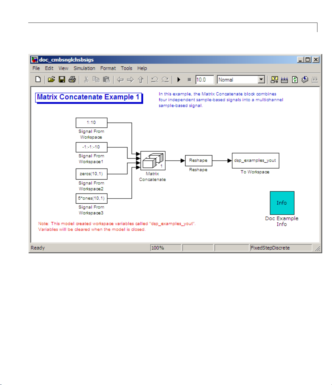
Combining Single-Channel Sample-Based Signals

You can combine individual sample-based signals into a multichannel signal by using the Matrix Concatenate block in the Simulink Math Operations library:

1 Open the Matrix Concatenate Example 1 model by typing

doc_cmbsnglchsbsigs

at the MATLAB command line.

Creating Multichannel Sample-Based Signals

2 Double-click the Signal From Workspace block, and set the Signal

parameter to

3 Doub

4 Double-click the Signal From Workspace2 block, and set the Signal

le-click the Signal From Workspace1 block, and set the Signal

meter to

para

parameter to

5 Double-click the Signal From Workspace3 block, and set the Signal

parameter to

1:10.ClickOK.

-1:-1:-10.ClickOK.

zeros(10,1).ClickOK.

5*ones(10,1).ClickOK.

1-33

1 Working with Signals

6 Double-click the Matrix Concatenate block. Set the block parameters as

follows, and then click OK:

• Number of inputs =

• Mode = Multidimensional array

• Concatenate dimension = 1

7 Double-click the Reshape block. Set the block parameters as follows, and

then click OK:

• Output dimensionality =

Customize

• Output dimensions = [2,2]

8 Run the model.

Four independent sample-based signals are combined into a 2-by-2

multichannel matrix signal.

Each 4-by-1 output from the Matrix Concatenate block contains one sample

from each of the four input signals at the same instant in time. The

Reshape block rearranges the samples into a 2-by-2 matrix. Each element

of this matrix is a separate channel.

Note that the Reshape block works columnwise, so that a column vector

input is reshaped as shown below.

1-34

The 4-by-1 matrix output by the Matrix Concatenate block and the 2-by-2

matrix output by the Reshape block in the above model represent the same

four-channel sample-based signal. In s ome cases, one representation of the

signal may be more useful than the other.

9 At the MATLAB command line, type dsp_examples_yout.

The four-channel, sample-based signal is displayed as a series of matrices

in the MATLAB Command Window. Note that the last matrix contains

Creating Multichannel Sample-Based Signals

only zeros. This is because every Signal From Workspace block in this

model has its Form output after final data value by parameter set

Setting to Zero.

Combining Multichannel Sample-Based Signals

You can combine existing multichannel sample-based signals into larger multichannel signals using the Simulink Matrix Concatenate block:

1 Open the Matrix Concatenate Example 2 model by typing

doc_cmbmltichsbsigs

at the MATLAB command line.

1-35

1 Working with Signals

1-36

2 Double-click the Signal From Workspace block, and set the Signal

parameter to

3 Double-click the Signal From Workspace1 block, and set the Signal

parameter to

4 Double-click the Matrix Concatenate block. Set the block parameters as

[1:10;-1:-1:-10]'.ClickOK.

[zeros(10,1) 5*ones(10,1)].ClickOK.

follows, and then click OK:

• Number of inputs =

• Mode = Multidimensional array

Creating Multichannel Sample-Based Signals

• Concatenate dimension = 1

5 Run the model.

The model combines both two-channel sample-based signals into a

four-channel signal.

Each 2-by-2 output from the Matrix Concatenate block contains both

samples from each of the two input signals at the same instant in time.

Each element of this matrix is a separate channel.

1-37

1 Working with Signals

Creating Multichannel Frame-Based Signals

In this section...

“Multichannel Frame-Based Signals” on page 1-38

“Combining Frame-Based Signals” on page 1-39

Multichannel Frame-Based Signals

A frame-based signal with N channels and frame size M is represented by a sequence of M-by-N matrices. Multiple individual frame-based signals, with the same frame rate and size, can be combined into a multichannel frame-based signal using the Simulink Matrix Concatenate block. Individual signals can be added to an existing multichannel signal in the same way.

1-38

Creating Multichannel F rame-Based Signals

Combining Frame

You can combine e signal by using t the same frame r frame-based si produce a thre

1 Open the Matri

doc_combiningfbsigs

at the MATLA

xisting frame-based signals into a larger multichannel

he Simulink Concatenate block. All signals must have

ate and frame s ize. In this example, a single-channel gnal is combined with a two-channel frame-based signal to e-channel frame-based signal:

x Concatenate Example 3 model by typing

B command line.

-Based Signals

1-39

1 Working with Signals

1-40

2 Double-click the Signal From Workspace block. Set the block parameters

as follows:

• Signal =

• Sample time = 1

• Samples per frame = 4

Based on these parameters, the Signal From Workspace block outputs a frame-based signal with a frame size of four.

3 Save these parameters and close the dialog box by clicking OK.

[1:10;-1:-1:-10]'

Creating Multichannel F rame-Based Signals

4 Double-click the Signal From Workspace1 block. Set the block parameters

as follows, and then click OK:

• Signal =

5*ones(10,1)

• Sample time = 1

• Samples per frame = 4

The Signal From Workspace1 block has the same sample time and frame size as the Signal From Workspace block. When yo u combine frame-based signals into multichannel signals, the original signals must have the same frame rate and frame size.

5 Double-click the Matrix Concatenate block. Set the block parameters as

follows, and then click OK:

• Number of inputs =

• Mode = Multidimensional array

• Concatenate dimension = 2

6 Run the model.

The 4-by-3 matrix output from the Matrix Concatenate block contains all three input channels, and preserves their common frame rate and frame size.

1-41

1 Working with Signals

Deconstructing Multichannel Sample-Based Signals

In this section...

“Splitting Multichannel Sample-Based Signals into Individual Signals” on page 1-42

“Splitting Multichannel Sample-Based Signals into Several Multichannel Signals” on page 1-45

Splitting Multichannel Sample-Based Signals into Individual Signals

Multichannel signals, rep resen t ed by matrices in the Simul in k environment, are frequently used in signal processing models for efficiency and compactness. Though most of the signal processing blocks can process multichannel signals, you may need to access just one channel or a particular range of samples in a multichannel signal. You can access individual channels of the multichannel signal by using the blocks in the Indexing library. This library includes the Selector, Submatrix, Variable Selector, Multiport Selector, and Submatrix blocks.

1-42

You can split a multichannel sample-based signal into single-channel sample-based signals using the Multiport Selector block. This block allows you to select specific rows and/or columns and propagate the selection to a chosen output port. In this example, a three-channel sample-based signal is deconstructed into three independent sample-based signals:

1 Open the Multiport Selector Example 1 model by typing

doc_splitmltichsbsigsind at the MATLAB command line.

Deconstructing Multichannel Sample-Based Signals

2 Double-click the Signal From Workspace block, and set the block

parameters as follows:

• Signal =

randn(3,1,10)

• Sample time = 1

• Samples per frame = 1

ed on these parameters, the Signal From Workspace block outputs a

Bas

ee-channel, sample-based signal with a sample period of 1 second.

thr

3 Save these parameters and close the dialog box by clicking OK.

1-43

1 Working with Signals

4 Double-click the Multiport Selector block. Set the block parameters as

follows, and then click OK:

• Select =

Rows

• Indices to output = {1,2,3}

Based on these parameters, the M ultiport Selector block extracts the rows of the input. The Indices to output parameter setting sp ecifies that row 1 of the input should be reproduced at output 1, row 2 of the input should be reproduced at output 2, and row 3 of the input should be reproduced at output 3.

5 Run the model.

6 At the MATLAB command line, type dsp_examples_yout.

The following is a portion of what is displayed at the MATLAB command line. Because the input signal is random, your output might be different than the output show here.

dsp_examples_yout(:,:,1) =

-0.1199

dsp_examples_yout(:,:,2) =

-0.5955

1-44

dsp_examples_yout(:,:,3) =

-0.0793

This sample-based signal is the first row of the input to the Multiport Selector block. You can view the other two input rows by typing

dsp_examples_yout1 and dsp_examples_yout2,respectively.

You have now successfully created three, single-channel sample-based signals from a multichannel sample-based signal using a Multiport Selector block.

Deconstructing Multichannel Sample-Based Signals

Splitting Multi

channel Sample-Based Signals into

Several Multich

Multichannel si are frequently Though most of you may need to multichannel signal by usin Selector, Su blocks.

You can spli sample-bas most versat channel se sample-ba signal fro

1 Open the S

at the MAT

gnals, represented by matrices in the Simulink environment,

used in signal processing models for efficiency and compactness.

the signal processing blocks can process multichannel signals,

access just one channel or a particular range of samples in a signal. You can access individual channels of the multichannel g the blocks in the Indexing library. This library includes the

bmatrix, Variable Selector, Multiport Selector, and Submatrix

t a multichannel sample-based signal into other multichannel

ed signals using the Submatrix block. The Submatrix block is the

ile o f the blocks in the Indexing library because it allows arbitrary

lections. Therefore, you can extract a portion of a multichannel

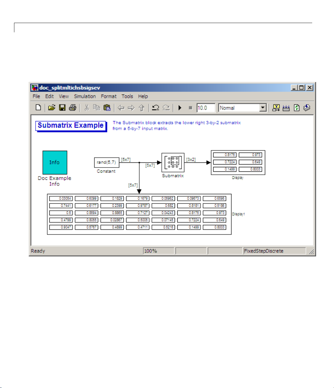
sed signal. In this example, you extract a six-channel, sample-based

m a 35-channel, sample-based signal (5-by-7 matrix):

ubmatrix Example model by typing

LAB command line.

annel Signals

doc_splitmltichsbsigsev

1-45

1 Working with Signals

1-46

2 Double

• Consta

• Inter

• Sampl

• Samp

-click the Constant block, and set the block parameters as follows:

nt value =

rand(5,7)

pret vector parameters as 1–D = Clear th is check box

ing mode =

le Time =

Sample based

Based on these parameters, the Constant block outputs a constant-valued, sample-based signal.

3 Save these parameters and close the dialog box by clicking OK.

ble-click the Submatrix block. Set the block parameters as follows,

4 Dou

dthenclickOK:

Deconstructing Multichannel Sample-Based Signals

• Row span = Range of rows

• Starting row = Index

• Starting row index = 3

• Ending row = Last

• Column span = Range of columns

• Starting column = Offset from last

• Starting column offset = 1

• Ending column = Last

Based on these parameters, the Submatrix block outputs rows three to five, the last row of the input signal. It also outputs the second to last column and the last column of the input signal.

1-47

1 Working with Signals

5 Run the model.

The model should now look similar to the following figure.

1-48

e that the output of the Submatrix block is equivalent to the matrix

Notic

ted by rows three through five and columns six through seven of the

crea

tmatrix.

inpu

ave now successfully created a six-channel, sample-based signal from a

You h

channel sample-based signal using a Submatrix block.

35-

Deconstructing Multichannel Frame-Based Signals

In this section...

“Splitting Multichannel Frame-Based Signals into Individual Signals” on page 1-49

“Reordering Channels in Multichannel Frame-Based Signals” on page 1-54

Splitting Multichannel Frame-Based Signals into Individual Signals

You can use the Multiport Selector block in the Indexing library to extract the individual channels of a multichannel frame-based signal. These signals form single-channel frame-based signals that have the same frame rate and size of the m ultichannel signal.

1-49

1 Working with Signals

The figure below is a graphical repre sentation of this process.

In this example, you use the Multiport Selector block to extract a single-channel and a two channel frame-based signal from a multichannel frame-based signal:

1-50

1 Open the Multiport Selector Example 2 model by typing

doc_splitmltichfbsigsind

at the MATLAB command line.

Deconstructing Multichannel Frame-Based Signals

2 Doubl

e-click the Signal From Workspace block, and set the block

param

• Sign

• Samp

eters as follows:

al =

[1:10;-1:-1:-10;5*ones(1,10)]'

les per frame =

Based on these parameters, the Signal From Workspace block outputs a three-channel, frame-based signal with a frame size of four.

3 Save these parameters and close the dialog box by clicking OK.

1-51

1 Working with Signals

4 Double-click the Multiport Selector block. Set the block parameters as

follows, and then click OK:

• Select =

• Indices to output = {[1 3],2}

Based on these parameters, the Multiport Selector block outputs the first andthirdcolumnsatthefirstoutputportandthesecondcolumnatthe second output port of the block. Setting the Select parameter to ensures that the block preserves the frame rate and frame size of the input.

5 Run the model.

The figure below is a graphical representation of how the Multiport Selector block splits one frame of the three-channel frame-based signal into a single-channel signal and a two-channel signal.

Columns

1-52

Deconstructing Multichannel Frame-Based Signals

The Multiport Selector block outputs a two-channel frame-based signal, comprised of the first and third column of the input signal, at the first port. It outputs a single-channel frame-based signal, comprised of the second column of the input signal, at the second port.

1-53

1 Working with Signals

You have now successfully created a single-channel and a two-channel frame-based signal from a multichannel frame-based signal using the Multiport Selector block.

Reordering Channels in Multichannel Frame-Based Signals

Multichannel signals, represented by matrices in Simulink, are frequently used in signal processing models for efficiency and compactness. Though most of the signal processing blocks can process multichannel signals, y ou may need to access just one channel or a particular range of samples in a multichannel signal. You can access individual channels of the multichannel signal by using the blocks in the Indexing library. This library includes the Selector, Submatrix, Variable Selector, Multiport Selector, and Submatrix blocks. ItisalsopossibletousethePermute Matrix block, in the Matrix operations library, to reorder the channels of a frame-based signal.

Some Signal Processing Blockset blocks have the ability to process the interaction of channels. Typically, Signal Processing Blockset blocks com pare channel one of signal A to channel one of signal B. However, you might want to correlate channel one of signal A with channel three of signal B. In this case, in order to compare the correct signals, you need to use the Permute Matrix block to rearrange the channels of your frame-based signals. This example explains how to accomplish this task:

1-54

1 Open the Permute Matrix Example model by typing

doc_reordermltichfbsigs at the MATLAB command line.

Deconstructing Multichannel Frame-Based Signals

2 Double-click the Signal From Workspace block, and set the block

parameters as follows:

• Signal =

[1:10;-1:-1:-10;5*ones(1,10)]'

• Sample time = 1

• Samples per frame = 4

Based on these parameters, the Signal From Workspace block outputs a three-channel, frame-based signal with a sample period of 1 second and a frame size of 4. The frame period of this block is 4 seconds.

3 Save these parameters and close the dialog box by clicking OK.

1-55

1 Working with Signals

4 Double-click the Constant block. Set the block parameters as follows, and

then click OK:

• Constant value =

[1 3 2]

• Interpret vector parameters as 1–D = Clear th is check box

• Sampling mode =

Frame based

• Frame period = 4

The discrete-time, frame-based vector output by the Constant block tells the Permute Matrix block to swap the second and third columns of the input signal. Note that the frame period of the Constant block must match the frame period of the Signal From Workspace block.

5 Double-click the Permute Matrix block. Set the block parameters as

follows, and then click OK:

• Permute =

Columns

• Index mode = One-based

Based on these parameters, the Permute Matrix block rearranges the columns of the input signal, and the index of the first column is now one.

6 Run the model.

The f igure below is a graphical representation of what happens to the first input frame during sim u la tion.

1-56

Deconstructing Multichannel Frame-Based Signals

The second and third channel of the frame-based input signal are swapped.

7 At the MATLAB command line, type yout.

You can now verify that the second and third columns of the input signal are rearranged.

You have now successfully reordered the channels of a frame-based signal using the Permute Matrix block.

1-57

1 Working with Signals

Importing and Exporting Sample-Based Signals

In this section...

“Importing Sample-Based Vector Signals” on page 1-58

“Importing Sample-Based Matrix Signals” on page 1-61

“Exporting Sample-Based Signals” on page 1-65

Importing Sample-Based Vector Signals

The Signal From Workspace block generate s a sample-based vector signal when the variable or expression in the Signal parameter is a matrix and the Samples per frame parameter is set to represents a different channel. Beginning with the first row of the matrix, the block outputs one row of the matrix at each sample time. Therefore, if the Signal parameter specifies an M-by-N matrix, the output of the Signal From Workspace block is M 1-by-N row vectors representing N channels.

1.Eachcolumnoftheinputmatrix

1-58

Importing and Exporting Sample-Based Signals

The figure below is a graphical representation of this pro cess for a 6-by-4 workspace matrix,

In the following example, you use the Signal From Workspace block to import a sample-based vector signal into your model:

1 Open the Signal From Workspace Example 3 model by typing

doc_importsbvectorsigs at the MATLAB comm and line.

1-59

1 Working with Signals

1-60

2 At the MATLAB command line, type A = [1:100;-1:-1:-100]';

The matrix A represents a two column signal, where each column is a different channel.

3 At the MATLAB command line, type B = 5*ones(100,1);

The vector

4 Double-click the Signal From Workspace block, and set the block

B represents a single-channel signal.

parameters as follows:

• Signal =

[A B]

• Sample time = 1

• Samples per frame = 1

• Form output after final data value = Setting to zero

Importing and Exporting Sample-Based Signals

The Signal expression [A B] uses the standard MATLAB syntax for horizontally concatenating matrices a nd appends column vector right of matrix

A. The Signal From W orkspace block outputs a sample-based

B to the

signal with a sample period of 1 second. After the block has output the signal, all subsequent outputs have a value of zero.

5 Save these parameters and close the dialog box by clicking OK.

6 Run the model.

The following figure is a graphical representation of the model’s behavior during simulation.

The first row of the input matrix [AB]is output at time t=0, the second row o f the input matrix is output at time

t=1,andsoon.

You have now successfully imported a sample-based vector signal into your signal processing model using the Signal From Workspace block.

Importing Sample-Based Matrix Signals

The Signal From Workspace block generates a sample-based matrix signal when the variable or expression in the Signal parameter is a three-dimensional array and the Samples per frame parameter is set to Beginning with the first page of the array, the block outputs a single page of the array to the output at each sample time. Therefore, if the Signal parameter specifies an M-by-N-by-P array, the output of the Signal From Workspace block is P M-by-N matrices representing M*N channels.

1-61

1 Working with Signals

The f ol lowing f ig u re is a graphical illustration of this process for a 6-by-4-by-5 workspace array

1-62

In the following example, you use the Signal From Workspace block to import a four-channel, sample- based matrix signal into a Simulink model:

1 Open the Signal From Workspace Example 4 model by typing

doc_importsbmatrixsigs at the MATLAB comm and line.

Importing and Exporting Sample-Based Signals

Also, the following variables are loaded into the MATLAB workspace:

Fs 1x1 8 double array

dsp_examples_A 2x2x100 3200 double array

dsp_examples_sig1 1x1x100 800 double array

dsp_examples_sig12 1x2x100 1600 double array

dsp_examples_sig2 1x1x100 800 double array

dsp_examples_sig3 1x1x100 800 double array

dsp_examples_sig34 1x2x100 1600 double array

1-63

1 Working with Signals

dsp_examples_sig4 1x1x100 800 double array

mtlb 4001x1 32008 double array

2 Double-click the Signal From Workspace block. Set the block parameters

as follows, and then click OK:

• Signal =

dsp_examples_A

• Sample time = 1

• Samples per frame = 1

• Form output after final data value = Setting to zero

The dsp_examples_A array represents a four-channel, sample-based signal with 100 samples in each channel. This is the signal that you want to import, and it was created in the following way:

dsp_examples_sig1 = reshape(1:100,[1 1 100]) dsp_examples_sig2 = reshape(-1:-1:-100,[1 1 100]) dsp_examples_sig3 = zeros(1,1,100) dsp_examples_sig4 = 5*ones(1,1,100) dsp_examples_sig12 = cat(2,sig1,sig2) dsp_examples_sig34 = cat(2,sig3,sig4) dsp_examples_A = cat(1,sig12,sig34) % 2-by-2-by-100 array

3 Run the model.

Thefigurebelowisagraphicalrepresentation of the model’s behavior during simulation.

1-64

Importing and Exporting Sample-Based Signals

The Signal From Workspace block imports the four-channel sample based signal from the MATLAB workspace into the Simulink model one matrix at atime.

You have now successfully imported a sample-based matrix signal i n t o your model using the Signal From Workspace block.

Exporting Sample-Based Signals

The Signal To Workspace and Triggered To Works pace blocks are the primary blocks for exporting signals of all dimensions from a Simulink model to the MATLAB workspace.

1-65

1 Working with Signals

A sample-based signal, w ith M*N channels, is represented in Simulink as a sequence of M-by-N matrices. When the input to the Signal To Workspace block is a sample-based signal, the block creates an M-by-N-by-P array in the MATLAB works pace containing the P most recent samples from each channel. The number of pages, P, is specified by the Limit data points to last parameter. The newest samples are added at the end of the array.

The f ol lowing figure is the graphical illustration of this process using a 6-by-4 sample-based signal exported to workspace array

1-66

The workspace array always has time running along its third dimension, P. Samples are saved along the P dimension whether the input is a matrix, vector, or scalar (single channel case).

InthefollowingexampleyouuseaSignalToWorkspaceblocktoexporta sample-based matrix signal to the MATLAB workspace:

Importing and Exporting Sample-Based Signals

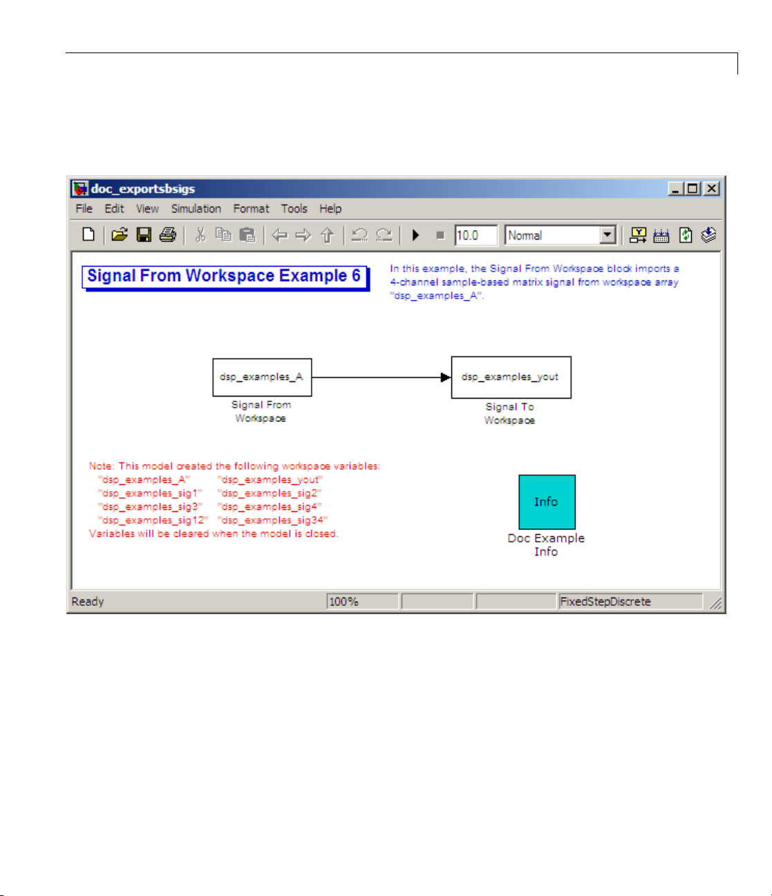
1 Open the Signal From Workspace Example 6 model by typing

doc_exportsbsigs at the MATLAB command line.

Also, the following variables are loaded into the MATLAB workspace:

dsp_examples_A 2x2x100 3200 double array

dsp_examples_sig1 1x1x100 800 double array

dsp_examples_sig12 1x2x100 1600 double array

dsp_examples_sig2 1x1x100 800 double array

dsp_examples_sig3 1x1x100 800 double array

1-67

1 Working with Signals

dsp_examples_sig34 1x2x100 1600 double array

dsp_examples_sig4 1x1x100 800 double array

In this model, the Signal From Workspace block imports a four-channel sample-based signal called

dsp_examples_A. This signal is then exported

to the MATLAB workspace using a Signal to Workspace block.

2 Double-click the Signal From Workspace block. Set the block parameters

as follows, and then click OK:

• Signal =

dsp_examples_A

• Sample time = 1

• Samples per frame = 1

• Form output after final data value = Setting to zero

Based on these parameters, the Signal From Workspace block outputs a sample-based signal with a sample period of 1 second. After the block has output the signal, all subsequent outputs have a value of zero.

3 Double-click the Signal To Workspace block. Set the block parameters as

follows, and then click OK:

• Variable name =

dsp_examples_yout

• Limit data points to last parameter to inf

• Decimation = 1

Based on these parameters, the Signal To Workspace block exports its sample-based input signal to a variable called

dsp_examples_yout in the

MATLAB workspace. The workspace variable can grow indefinitely large in order to capture all of the input data. The signal is not decimated before it is exported to the MATLAB workspace.

4 Run the model.

1-68

5 At the MATLAB command line, type dsp_examples_yout.

The four-channel sample-based signal,

dsp_examples_A,isoutputatthe

MATLAB command line. The following is a portion of the output that is displayed.

dsp_examples_yout(:,:,1) =

1-1 05

dsp_examples_yout(:,:,2) =

2-2 05

dsp_examples_yout(:,:,3) =

3-3 05

dsp_examples_yout(:,:,4) =

4-4 05

Importing and Exporting Sample-Based Signals

Each page of the output represents a different sample time, and each element of the matrices is in a separate channel.

You h ave now successfully exported a four-channel sample-based signal from a Simulink model to the MATLAB workspace us in g the Signal To Workspace block.

1-69

1 Working with Signals

Importing and Exporting Frame-Based Signals

In this section...

“Importing Fram e-Based Signals” on page 1-70

“Exporting Frame-Based Signals” on page 1-73

Importing Frame-Based Signals

The Signal From Workspace block creates a frame-based multichannel signal when the Signal parameter is a matrix, and the Samples per frame parameter, M, is greater than matrix, the block releases M rows of the matrix (that is, one frame from each channel) to the output port every M*T parameter s pecifies a W-by-N workspace matrix, the Signal From Workspace block outputs a series of M-by-N matrices representing N channels. The workspace matrix must be oriented so that its columns represent the channels of the signal.

1. Beginning with the first M rows of the

seconds. Therefore, if the Signal

1-70

The figure below is a graphical illustration of this process for a 6-by-4 workspace matrix,

A,andaframesizeof2.

Importing and Exporting Frame-Based Signals

Note Although independent channels are generally represented as columns, a single-channel signal can be represented in the workspace as either a column vector or row vector. The output from the Signal From Workspace block is a column vector in both cases.

In the following example, you u se the Signal From W orkspace block to create a three -channe l frame-based signal and import it into the model:

1 Open the Signal From Workspace Example 5 model b y typing

doc_importfbsigs

at the MATLAB command line.

dsp_examples_A = [1:100;-1:-1:-100]'; % 100-by-2 matrix dsp_examples_B = 5*ones(100,1); % 100-by-1 column vector

The variable called dsp_examples_A represents a two-channel signal with 100 samples, and the variable called dsp_exam ples_

B represents a

one-channel signal with 100 samples.

Also, the following variables are defined in the MATLAB workspace:

1-71

1 Working with Signals

1-72

2 Double-click the Signal From Workspace block. Set the block parameters

as follows, and then click OK:

• Signal parameter to

• Sample time parameter to 1

• Samples per frame parameter to 4

• Form output after final data value parameter to Setting to zero

Based on these parameters, the Signal From Workspace block outputs aframe-basedsignalwithaframesizeof4andasampleperiodof1 second. The signal’s frame period is 4 seconds. The Signal parameter uses the standard MATLAB syntax for horizontally concatenating matrices to append column vector

dsp_examples_A. After the block has output the signal, all subsequent

outputshaveavalueofzero.

[dsp_examples_A dsp_examples_B]

dsp_examples_B to the right of matrix

Importing and Exporting Frame-Based Signals

3 Run the model.

Thefigurebelowisagraphicalrepresentation of how your three-channel, frame-based signal is imported into your model.

You have now successfully imported a three-channel frame-based signal into your model using the Signal From Workspace block.

Exporting Frame-Based Signals

The Signal To Workspace and Triggered To Works pace blocks are the primary blocks for exporting signals of all dimensions from a Simulink model to the MATLAB workspace.

Aframe-basedsignalwithN channels and frame size M is represented by a sequence of M-by-N matrices. When the input to the Signal To Workspace block is a frame-based signal, the block creates a P-b y-N array in the MATLAB workspace containing the P most recent samples from each channel. The number of rows, P,isspecifiedbytheLimit data points to last parameter. The newest samples are added at the bottom of the matrix.

1-73

1 Working with Signals

The following figure is a graphical illustration of this pro cess for three consecutive frames of a frame-based signal with a frame size of 2 that is exported to matrix

A in the MATLAB workspace.

1-74

In the fol frame-b

1 Open the

doc_ex

lowing example, you use a Signal To Workspace block to export a

ased signal to the MATLAB workspace:

Signal From Workspace Example 7 model by typing

portfbsigs

at the MATLAB command line.

Importing and Exporting Frame-Based Signals

Also, th

The variable called dsp_examples_ with 100 samples, and the variable called dsp_exam ples_

e following variables are defined in the MATLAB workspace:

A represents a two-channel signal

B represents a

one-channel signal with 100 samples.

dsp_examples_A = [1:100;-1:-1:-100]'; % 100-by-2 matrix dsp_examples_B = 5*ones(100,1); % 100-by-1 column vector

2 Double-click the Signal From Workspace block. Set the block parameters

as follows, and then click OK:

• Signal =

[dsp_examples_A dsp_examples_B]

• Sample time = 1

• Samples per frame = 4

• Form output after final data value = Setting to zero

1-75

1 Working with Signals

dsp_examples_A. After the block has output the signal, all subsequent

dsp_examples_B to the right of matrix

outputshaveavalueofzero.

3 Double-click the Signal To Workspace block. Set the block parameters as

follows, and then click OK:

• Variable name =

dsp_examples_yout

• Limit data points to last = inf

• Decimation = 1

• Frames = Concatenate frames (2-D array)

Based on these parameters, the Signal To Workspace block exports its frame-based input sig n al to a varia ble called

dsp_examples_yout in the

MATLAB workspace. The workspace variable can grow indefinitely large in order to capture all of the input data. The signal is not decimated before it is exported to the MATLAB workspace, and each input frame is vertically concatenated to the previous frame to produce a 2-D array output.

4 Run the model.

The following figure is a graphical representation of the model’s behavior during simulation.

1-76

Importing and Exporting Frame-Based Signals

5 At the MATLAB command line, type dsp_examples_yout.

The output is shown below:

dsp_examples_yout =

1-1 5 2-2 5 3-3 5 4-4 5 5-5 5 6-6 5 7-7 5 8-8 5

9-9 5 10 -10 5 11 -11 5 12 -12 5

1-77

1 Working with Signals

Theframesofthesignalareconcatenated to form a two-dimensional array.

You have now successfully output a frame-based signal to the MATLAB workspace using the Signal To Workspace block.

1-78

Displaying Time-Domain Data

You can use Signal Processing Blockset blocks to work with signals in both the time and frequency domain. The Signal Processing Sinks library contains the following blocks for displaying time-domain signals:

• Time Scope

• Vector Scope

• Matrix Viewer

• Waterfall Scope

See the following sections for examples of how you can use the Vector Scope and Time Scope blocks to display time-domain data:

• “Displayin g Time Domain Data in the Vector Scope” on page 1-79

• “Displaying Time-Domain Data in the Time Scope” on page 1-82

Displaying Time-Domain Data

Displaying Time Domain Data in the Vector Scope

The following example shows you how you can use the Vector Scope block to display time-domain signals:

1 At the MATLAB command prompt, type doc_vectorscope_tut.

The Vector Scope Example opens and the variables into the MATLAB workspace.

Fs and mtlb are loaded

1-79

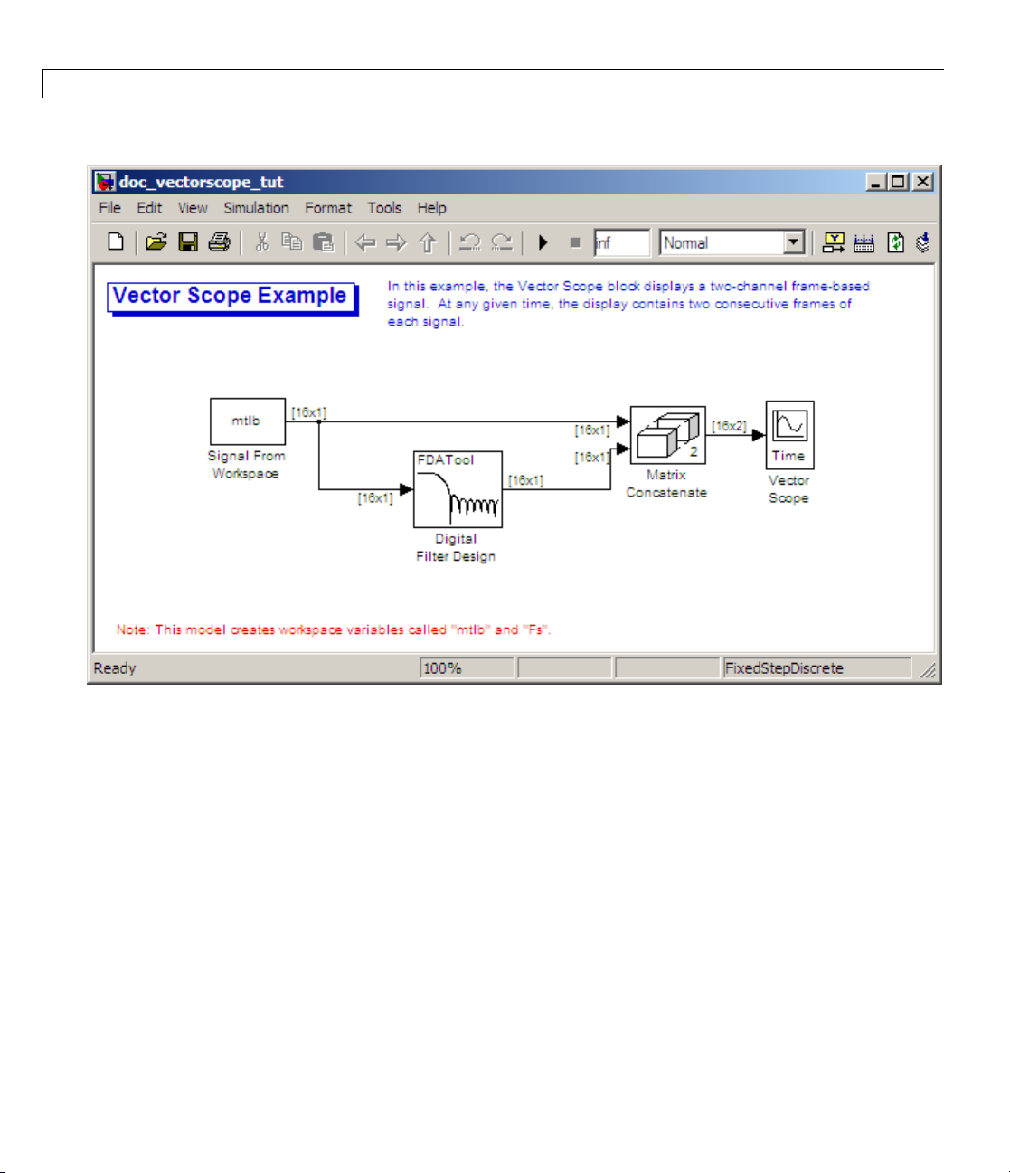
1 Working with Signals

1-80

2 Double-click the Signal From Workspace block. The Block Parameters:

Signal From Workspace dialog box opens.

3 Set the

• Signa

• Sampl

• Samp

• Form

block parameters as follows:

l =

mtlb

etime=

les per frame =

output after final data value =

Cyclic Repetition

Based on these parameters, the Signal From Workspace block outputs a frame-basedsignalwithaframesizeof16andasampleperiodof1second. The frame period of the signal is 16 seconds. Your input signal is output repeatedly from the Signal From Workspace block.

Displaying Time-Domain Data

4 Save these parameters and close the dialog box by clicking OK.

5 Double-click the Digital Fi lter Design block.

You are going to use this block to f ilter the input signal in order to produce two distinct signals to send to the Vector Scope block.

6 To specify a lowpass filter, in the Response Type section, choose Lowpass.

7 In the Design Method section, choose FIR. Then, from the list, select

Window.

8 In the Filter Order section, select Specify order and enter 22.

9 From the Window list, select Hamming.

10 In the Frequency Specifications section, from the Units list, select

Normalized (0 to 1).

11 In the Frequency Specifications section, set the wc parameter to 0.25.

12 Click Design Filter. Then, close the Block Parameters: Digital Filter

Design dialog box.

13 Double-click the Matrix Concatenate block. The Function Block

Parameters: Matrix Concatenate dialog box opens.

14 Set the block parameters as follows:

• Number of inputs =

• Mode = Multidimensional array.

• Concatenate dimension =

Based on these parameters, the Matrix Concatenate block combines the two signals so that each column corresponds to a different signal.

15 Save these parameters and close the dialog box by clicking OK.

16 Double-click the Vector Scope block.

17 Set the block parameters as follows, and then click OK:

1-81

1 Working with Signals

• Click the Scope Properties tab.

• Input domain =

• Time display span (number of frames) = 2

When you run the model, the Vector Scope block plots two consecutive frames of each channel at each update.

18 Run the model.

The Vector Scope window displays the original signal in blue and the filtered signal in black. To display the channel legend, right-click inside of the Vector Scope window and select Channel legend from the menu.

You have now successfully displayed two frame-based signals in the time domain using the Vector Scope block.

Time

Displaying Time-Domain Data in the Time Scope

Thefollowingexampleshowsyouhowtoconfigure the Time Scope blocks in the d oc_timesco pe _tut model to display time-domain signals.

1-82

Displaying Time-Domain Data

The Time Scope – Configuration dialog box provides a central location from which you can change the appearance and behavior of the Time Scope block. To open the Time Scope – Configuration dialog box, double-click the Time Scope block in your model and select File > Configuration.

1-83

1 Working with Signals

The Time Scope – Configuration dialog box has three different tabs, Core, Visuals,andTools, each of which offers you a different set of options. For

more information about the options available on e ach of the tabs, see the Time Scope reference page.

1-84

Example W

orkflow

Use the following workflow to configure the Time Scope blocks in the

doc_timescope_tut model:

1 “ConfiguringtheTimeScope”onpage1-85

2 “Using

3 “Modifying the Scope Display” on page 1-91

4 “Inspecting Your Data (Scaling the Axes and Zooming)” on page 1-94

5 “Man

To ge at t

the Playback Controls” on page 1-89

aging M ultiple Time Scopes” on page 1-97

t started with this example, open the model by typing doc_timescope_tut

he MATLAB command line.

Displaying Time-Domain Data

Configuring the Time Scope

To open the Time Scope – Configuration dialog box, you mu st first open the Time Scope window by double-clicking the Time Scope block in your model. When the window opens, select File > Configuration.

First, you configure the appearance of the Time Scope window and specify how the Time Scope block should interpret input signals using the Time Scope – Visuals:Time Domain Options dialog box.

Note As you progress through this workflow, notice the blue question mark

icon (

) in the lower-left corner of the subsequent dialog box es. This icon indicates that context-sensitive help is available. You can get more information about any of the parameters on the dialog box by right-clicking the parameter name and selecting What’s This?

Configuring Appearance and Specifying Signal Interpretation. To configure the appearance of the Time Scope window and specify how the Time Scope block interprets input signals:

1 Click the Visuals tab of the main Time Scope – Configuration dialog

box.

2 Select Time Domain, and click the Options button.

The following options dialog box appears.

1-85

1 Working with Signals

This table shows the appropriate parameter settings for the Main tab of the Visuals:Time Domain Options dialog box.

1-86

Parameter

Input Processing

Show grid Checked

Channel legend Checked

The Time Scope block accepts both sample- and frame-based input signals, but you must specify how the b lock should handle them. To do so, set the Input processing parameter on the Time Scope – Visuals:Time Domain Options dialog box to the appropriate choice.

In this example, you want the block to treat the input signal as frame based, so you must set the Input processing parameter to

channels (Frame-based)

Setting Axis Properties. Navigate to the Axis Properties tab of the Visuals:Time Domain O ptions dialog box, and set the parameters to the

values shown in the following table.

Setting

Columns as channels (Frame-based)

Columns as

Displaying Time-Domain Data

Parameter

Time range

Time display offset

Minimum Y-limit

Maximum Y-limit

Y-axis label

Setting

Input sample time

-2.5

2.5

Amplitude

The Time range parameter allows you to enter a numeric value, a variable that evaluates to a numeric value, or select the

Input sample time menu

option. The actual range of values that the block displays on the X-axis depends on the value of b oth the Time range and Time display offset parameters. See the following figure.

For information on the other labels in thescopewindow,seetheTimeScope reference page. In this example, the values on the X-axis range from the

Input sample time,wheretheInput sample time is 0.05 seconds (50

0 to

ms). Click OK to save your changes and close the Visuals:Time Domain Options dialog box.

1-87

1 Working with Signals

Configuring Axis Scaling and Data Alignment. The Plot Navigation

options for the Time Scope block allow you to control when and how the block scales the axes. These options also control how the block aligns your data with respect to the axes. The following table describes these options.

Parameter

Axis scaling Allows you to specify when the block should

Data range (%) Allows you to s pecify how much white space

Align Allows you to specify where the block should

Description

scaletheaxes. Youcanchoosetoscale the axes manually, allow the scope to automatically scale the a xes when simulation stops, or allow scaling as needed throughout simulation.

surrounds your signal in the scope window. You can specify a value for both the Y- and X-axis. The higher the value you enter for the Y-axis Data range (%),thetighterthe Y-axis range is with respect to the minimum and maximum values in your signal. For example, to have your signal cover the entire Y-axis range when the block scales the axes, set this value to

align your data with respect to each axis. You can choose t o have your data aligned with the top, bottom, or center of the Y-axis. Additionally, if you select the Scale X-axis limits check box, you can choose to have your data aligned with the right, left, or center of the X-axis.

100.

1-88

1 To open the Plot Navigation options dialog box, navigate to the Tools

tab of the main configuration dialog box, and click Options.

Mathworks SIGNAL PROCESSING BLOCKSET 7 user guide

Specifications and Main Features

Frequently Asked Questions

User Manual

Working with Signals

Discrete-Time Signals

Time and Frequency Terminology

Recommended Settings for Discrete-Time Simulations

Other Settings for Discrete-Time Simulations

Cross-Rate Operations

Continuous-Time Signals

Continuous-Time Source Blocks

Continuous-Time Nonsource Blocks

Sample-Based Signals

Sample-Based Single Chan nel Signals

Sample-Based Multichannel Signals

Frame-Based Signals

Frame-Based Single Channel Signals

Frame-Based M ultichannel Signals

Benefits of Frame-Based Processing

Accelerating Real-Time Systems

Accelerating Simulations

Creating Sample-Based Signals

Using the Constant Block

Creating a 1-D Vector Signal

Using the Signal from Workspace Block

Creating Frame-Based Signals

Using the Sine Wave Block

Using the Signal from Workspace Block

Creating Multichannel Sample-Based Signals

Multichannel Sample-Based Signals

Combining Single-Channel Sample-Based Signals

Combining Multichannel Sample-Based Signals

Creating Multichannel Frame-Based Signals

Multichannel Frame-Based Signals

Deconstructing Multichannel Sample-Based Signals

Deconstructing Multichannel Frame-Based Signals

Reordering Channels in Multichannel Frame-Based Signals

Importing and Exporting Sample-Based Signals

Importing Sample-Based Vector Signals

Importing Sample-Based Matrix Signals

Exporting Sample-Based Signals

Importing and Exporting Frame-Based Signals

Importing Frame-Based Signals

Exporting Frame-Based Signals

Displaying Time-Domain Data

Displaying Time Domain Data in the Vector Scope

Displaying Time-Domain Data in the Time Scope

Configuring the Time Scope