


Signal Processing
Getting Star ted Guide
Blockset™ 7

How to Contact The MathWorks
www.mathworks.
comp.soft-sys.matlab Newsgroup
www.mathworks.com/contact_TS.html Technical Support
suggest@mathworks.com Product enhancement suggestions
bugs@mathwo
doc@mathworks.com Documentation error reports
service@mathworks.com Order status, license renewals, passcodes
info@mathwo
com
rks.com
rks.com
Web
Bug reports
Sales, prici
ng, and general information
508-647-7000 (Phone)
508-647-7001 (Fax)
The MathWorks, Inc.
3 Apple Hill Drive
Natick, MA 01760-2098
For contact information about worldwide offices, see the MathWorks Web site.
Signal Processing Blockset™ Getting Started Guide
© COPY R IGHT 2004–2010 The MathW orks, Inc.
The software described in this document is furnished under a license agreement. The software may be used
or copied only under the terms of the license agreement. No part of this manual may be photocopied or
reproduced in any form without prior written consent from The MathW orks, Inc.
FEDERAL ACQUISITION: This provision applies to all acquisitions of the Program and Documentation
by, for, or through the federal government of the United States. By accepting delivery of the Program
or Documentation, the government hereby agrees that this s oftware or docume n tation qualifies as
commercial computer software or commercial computer software documentation as such terms are used
or defined in FAR 12.212, DFARS Part 227.72, and DFARS 252.227-7014. Accordingly, the terms and
conditions of this Agreement and only those rights specified in this Agreement, shall pertain to and govern
theuse,modification,reproduction,release,performance,display,anddisclosureoftheProgramand
Documentation by the federal government (or other entity acquiring for or through the federal government)
and shall supersede any conflicting contractual terms or conditions. If this License fails to meet the
government’s needs or is inconsistent in any respect with federal procurement law, the government agrees
to return the Program and Docu mentation, unused, to The MathWorks, Inc.
Trademarks
MATLAB and Simulink are registered trademarks of The MathWorks, Inc. See
www.mathworks.com/trademarks for a list of additional trademarks. Other product or brand
names may be trademarks or registered trademarks of their respective holders.
Patents
The MathWorks products are protected by one or more U.S. patents. Please see
www.mathworks.com/patents for more information.

Revision History
June 2004 First printing New for Version 6.0 (Release 14)
October 2004 Second printing Revised for Version 6.0.1 (Release 14SP1)
March 2005 Online only Revised for Version 6.1 (Release 14SP2)
September 2005 Online only Revised for Version 6.2 (Release 14SP3)
March 2006 Online only Revised for Version 6.3 (Release 2006a)
September 2006 Online only Revised for Version 6.4 (Release 2006b)
March 2007 Online only Revised for Version 6.5 (Release 2007a)
September 2007 Third Printing Revised for Version 6.6 (Release 2007b)
March 2008 Fourth Printing Revised for Version 6.7 (Release 2008a)
October 2008 Online only Revised for Version 6.8 (Release 2008b)
March 2009 Online only Revised for Version 6.9 (Release 2009a)
September 2009 Online only Revised for Version 6.10 (Release 2009b)
March 2010 Online only Revised for Version 7.0 (Release 2010a)


Introduction
1
Product Overview ................................. 1-2
Contents
System Setup
Installation
Required Products
Related P roducts
Product Demos
Demos in the Help Browser
Demos on the Web
Demos on MATLAB Central
Working with the Documentation
Viewing the Documentation
Printing the Documentation
Using This Guide
...................................... 1-3
...................................... 1-3
................................. 1-3
.................................. 1-4
.................................... 1-5
......................... 1-5
................................. 1-10
......................... 1-11
................... 1-12
......................... 1-12
......................... 1-13
................................. 1-13
Concepts, Terminology, and Feature Overview
2
Sample Model and Block Libraries .................. 2-2
Modeling System Behavior
Signal Processing Blockset Blocks
.......................... 2-2
.................... 2-5
Key Blockset Concepts
Signals
Sample Time
State
Sample-Based Signals
Frame-Based Signals
.......................................... 2-10
..................................... 2-10
............................................ 2-11
............................. 2-10
.............................. 2-11
.............................. 2-12
v

Tunable Parameters ............................... 2-14
Signal Processing Blockset Product Features
Frame-Based Operations
Multirate Processing
Fixed-Point Support
Real-Time Code Generation
Adaptive and Multirate Filtering
Quantization
Statistical Operations
Linear Algebra
Parametric Estimation
Matrix Support
Data Type Support
Configuring the Simulink Environment for Signal
Processing Models
Using dspstartup.m
Settings in dspstartup.m
..................................... 2-18
.................................... 2-19
................................... 2-20
........................... 2-16
............................... 2-17
............................... 2-17
......................... 2-18
..................... 2-18
.............................. 2-19
............................. 2-19
................................ 2-20
............................... 2-23
................................ 2-23
........................... 2-24
Signal Processing Models
3
........ 2-16
vi Contents
Creating a Block Diagram .......................... 3-2
Setting the Model Parameters
Running the Model
Modifying Your Model
................................ 3-9
............................. 3-12
...................... 3-6
4
Digital Filters ..................................... 4-2
Filters

Designing a Digital Filter ........................... 4-2
Adding a Digital Filter to Your Model
................. 4-6
Adaptive Filters
Designing an Adaptive Filter
Adding the Adaptive Filter to Your Model
Viewing the Coefficients of Your Adaptive Filter
................................... 4-9
........................ 4-9
............. 4-14
........ 4-19
Code Generation
5
Understanding Code Gener a tio n .................... 5-2
Code Generation with the Real-Time Workshop Product
Highly Optimized Generated ANSI C Code
Generating Code
SettingUptheBuildFolder
Setting Configuration Parameters
Generating Code
Viewing the Generated Code
.................................. 5-4
......................... 5-4
.................... 5-5
.................................. 5-10
........................ 5-11
............. 5-3
.. 5-2
Frequency Domain Signals
6
Power Spectrum Estimates ......................... 6-2
Creating the Block Diagram
Setting the Model Parameters
Viewing the Power Spectrum Estimates
Spectrograms
Modifying the Block Diagram
Setting the Model Parameters
Viewing the Spectrogram of the Speech Signal
..................................... 6-12
......................... 6-2
....................... 6-3
............... 6-9
........................ 6-12
....................... 6-14
.......... 6-18
vii

Index
viii Contents

Introduction
• “Product Overview” on page 1-2
• “System Setup” on page 1-3
• “Product Demos” on page 1-5
• “Working with the Documentation” on page 1-12
1

1 Introduction
Product Overview
Signal Processing Blockset™ provides algorithms a nd tools for the design and
simulation of signal processing systems. You can develop DSP algorithms
for speech and audio processing, signal detection, radar tracking, baseband
communications, and other applications. Most algorithms and tools are
available as both System objects (for use in MATLAB
Simulink
The blockset provides techniques for FFTs, FIR and IIR digital filtering,
spectral estim ation, statistical and linear algebra computations, streaming,
and multirate processing. It also includes signal generators, interactive
scopes, spectrum analyzers, and other tools for visualizing signals and
simulation results.
You can use the blockset to develop and validate real-time signal processing
systems. For embedded system design and rapid prototyping, the blockset
supports fixed-point arithmetic, C-code generation, and implementation on
embedded hardware.
®
®
).
) and blocks (for use in
1-2

System Setup
Installation
Before you begin working, you need to install the product on your computer.
Installing the Signal Processing Blockset Software
The Signal Processing Blockset software follows the same installation
procedure as the MATLAB toolboxes. See the MATLAB installation
documentation for your platform.
System Setup
In this section...
“Installation” on page 1-3
“Required Products” on page 1-3
“Related Products” on page 1-4
Installing Online Documentation
Installing the documentation is part of the installation process:
• Installation from a DVD — Start the MathWorks™ installer. When
prompted, select the Product check boxes for the products you want to
install. The documentation is installed along with the products.
• Installation from a Web download — If you update the Signal Processing
Blockset software using a Web download and you want to view the
documentation with the MATLA B Help browser, you must install the
documentation on your hard drive.
Download the files from the Web. Then, start the installer, and select
the Product check boxes for the products you want to install. The
documentation is installed along with the products.
Required Products
The Signal Processing Blockset product is part of a family of products from The
MathWorks™. You need to install the following products to use the blockset:
1-3

1 Introduction
• MATLAB — You use MATLAB to open model files and view Signal
Processing Blockset demos. You can import signal values from the
MATLAB workspace into signal processing models and export signal values
from signal processing models to the MATLA B workspace.
• Simulink — Simulink provides an environment that enables you to create a
block diagram to model your physical system. You can create these block
diagrams by connecting blocks and using graphical user interfaces (GUIs)
to edit block parameters.
• Signal Processing Toolbox™ — The Signal Processing To olbox product
provides basic filter capabilities. You can design and implement filters
using the Filter Design and Analysis Tool (FDATool) and use them in your
signal processing models.
Related Products
The MathWorks provides several products that are relevant to the kinds of
tasks you can perform with Signal Processing Blockset softw are.
For more information about any of these products, see either
1-4
• The online documentation for that product if it is installed on your system
• The MathWorks Web site, at
http://www.mathworks.com/products/sigprocblockset/related.jsp

Product Demos
In this section...
“Demos in the Help Browser” on page 1-5
“Demos on the Web” on page 1-10
“Demos on MATLAB Central” on p age 1-11
Demos in the Help Browser
You can find interactive Signal P ro cessing Blockset demos in the MATLAB
Help browser. This example show s you how to locate and open some typical
demos:
1 To open the Help browser, type doc at the MATLAB command line.
2 Expand the Signal Processing Blockset node in the Help browser, then
the Demos node.
Product Demos
1-5

1 Intr oduc tion
1-6
There are two entries under the Signal Processing Blockset Demos node:
• Simulink Demos — Expand this entry to see a categorical list of
block-based Signal Processing Blockset demos.
• MATLAB Demos — Expand this entry to see a categorical list of Signal
Processing Blockset System object demos.
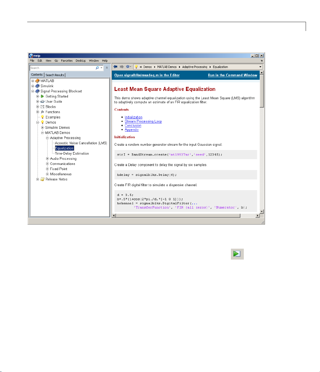
3 To view the description of the Simulink-based Equalization demo, which
demonstrates adaptive channel equalization, expand the Simulink Demos
and Adaptive Processing nodes, then click Equalization.

Product Demos
a Click Open this model to display the Simulink mod el for the
Equalization demo. The model window opens, and a Results window
opens to display the simulation results.
1-7

1 Intr oduc tion
1-8
b Run the model by selecting Start from the Simulation menu in the
model window. The results of the simulation appear in the Results
window.
4 To view
MATLAB
nodes,
a version of the Equalization d emo that uses System objects in
,expandtheMATLAB Demos and Adaptive Processing
then click Equalization.
Product Demos
a Click Open signalblkslmsadeq.m in the Editor to display the System
object Equalization demo in the MATLAB editor.
b Run the demo by clicking the Run toolbar button ( ). The results of
thedemoappearinthefollowingfigure.
1-9

1 Intr oduc tion
1-10
Demos on the Web
The MathWorks Web site contains demos that show you how to use
Signal Processing Blockset software. You can find these demos at
http://www.mathworks.com/products/sigprocblockset/demos.jsp.
You can run these demos without having MATLAB or the Signal Processing
Blockset product installed on your system.

Product Demos
Demos on MATLAB C
MATLAB Central c
developers of Si
products. Cont
browse these ca
Blockset soft
Central is loc
ware or a specific problem that you want to solve. MATLAB
ontains files, including demos, contributed by users and
gnal Processing Blockset, MATLAB, Simulink, and other
ributors submit their files to one o f a list of categories. You can
tegories to find submissions that pertain to Signal Processing
ated at
http://www.mathworks.com/matlabcentral/.
entral
1-11

1 Intr oduc tion
Working with the Documentation
In this section...
“Viewing the Documentation” on page 1-12
“Printing the Documentation” on page 1-13
“Using This Guide” on pag e 1-13
Viewing the Documentation
You can access the Signal Processing Blockset documentation using files you
installed on your system or from the Web using the MathWorks Web site.
DocumentationintheHelpBrowser
This procedure shows you how to use the Help browser to view the blockset
documentation installed on your system:
1 In the MATLAB window, from the Help menu, click Product Help.The
Help browser opens.
1-12
2 From the list of products in the left pane, click Signal Processing
Blockset. In the right pane, the Help browser displays the Signal
Processing Blockset roadmap page.
3 Under
Help b
the section titled Documentation Set,clickGetting Started.The
rowser displays the chapters of this manual.
DocumentationontheWeb
an also view the documentation from the MathWorks Web site. The
You c
mentation available on these Web pages is for the latest release,
docu
rdless of whether the release was distributed on a DVD or as a Web
rega
nload:
dow
igatetotheProductPageat
1 Nav
p://www.mathworks.com/products/sigprocblockset/
htt
2 Click the Documentation link on the left side of the page. The blockset
documentation is displayed.
.

Working with the Documentation
Printing the Doc
The Signal Proce
PDF format. To vi
1 In the MATLAB wi
Help browser o
2 From the list of products in the left pane, click Signal Processing
Blockset. In the right pane, the Help browser displays the Signal
Processing Blockset roadmap page.
3 Under the Printable (PDF) Documentation on the Web section, click
the links to view PDF versions of the blockset documentation.
ssing Blockset documentation is also available in printable
umentation
ew the documentation in PDF format:
ndow, from the Help menu, click Product Help.The
pens.
Using This Guide
To help you effectively read and use this guide, here is a brief description of
the chapters and a suggested reading path.
Expected
This manual assumes that you are already familiar with the following
products:
• MATLAB, to write scripts and functions, and to use functions with the
command-line interface
Background
• Simulink,tocreatesimplemodelsas block diagrams and simulate those
models
What C
If You Are a New User — In the Getting Started Guide:
• Read Chapter 1, “Introduction” to learn about the installation process, the
products required to run Signal Processing Blockset software, and how
to view the blockset demos.
• Read Chapter 2, “Concepts, Terminology, and Feature Overview” to learn
about blockset functionality, review key concepts and terminology, and find
out more about product features.
hapters Should I Read?
1-13

1 Intr oduc tion
• Read Chapter 3, “Signal Processing Models” to learn how to build a signal
processing model and simulate its behavior.
• Read Chapter 4, “Filters” to create an adaptive noise cancellation system
using digital and adaptive filters.
• Read Chapter 5, “Code Generation” to generate ANSI
signal processing model.
• Read Chapter 6, “Frequency Domain Signals” to learn how to view the
spectral content of a speech signal.
If You Are an Experienced User — In the User’s Guide:
• Read Chapter 1, “Working with Signals” and Chapter 2, “Advanced Signal
Concepts” for details on key operations common to many signal processing
tasks.
• Read the following chapters for discussions of how to implement various
signal processing operations:
®
C code from your
- Chapter 3, “Filters”
1-14
- Chapter 4, “Transforms”
- Chapter 5, “Quantizers”
- Chapter 6, “Statistics, Estimation, and Linear Algebra”
- Chapter 7, “Working with Fixed-Point Data”
• See the block reference for a description of each block’s operation,
parameters, and characteristics.

2
Concepts, Terminology, and Feature Overview
• “Sample Model and Block Libraries” on page 2-2
• “Key Blockset Concepts” on page 2-10
• “Signal Processing Blockset Product Features” on page 2-16
• “Configuring the Simulink Environment for Signal Processing Models”
on page 2-23

2 Concepts,Terminology,andFeatureOverview
Sample Model and Block Libraries
In this section...
“Modeling System Behavior” on page 2-2
“Signal Processing Blockset Blocks” on page 2-5
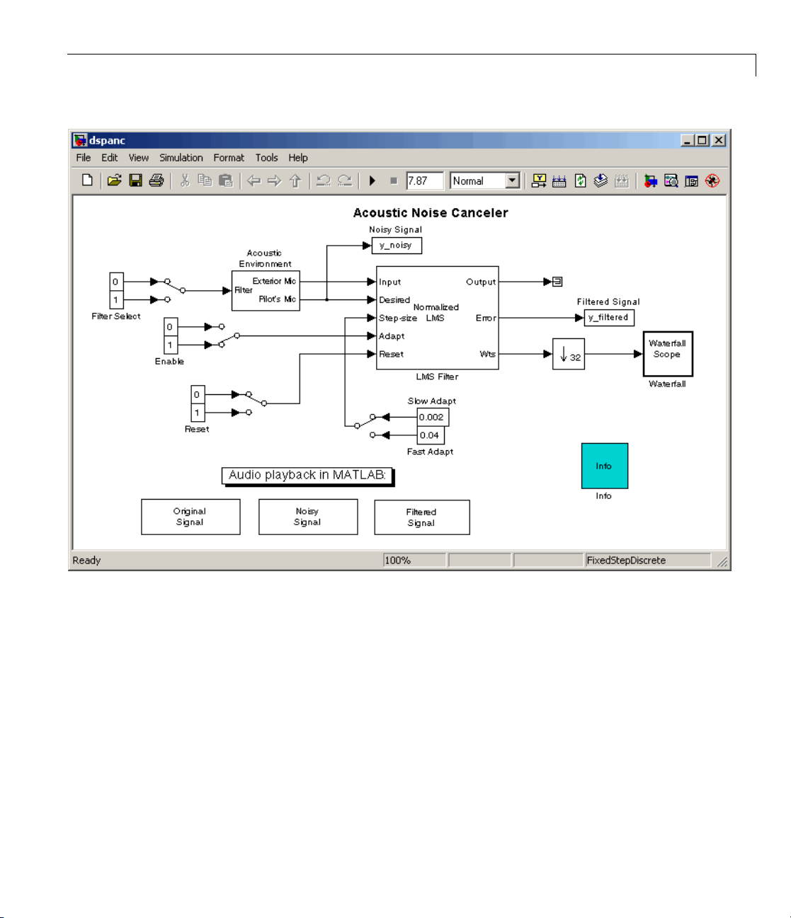
Modeling System Behavior
Signal Processing Blockset blocks can simulate the behavior of complex signal
processing systems. For example, the Acoustic Noise Canceler demo model in
this section illustrates some of the capabilities of the blockset. In the mode l,
the signal output at the upper port of the Acoustic Environment subsystem
is white noise. The signal output at the lower port contains colored noise
and a signal from a
remove the noise from the signal output at the lower port. When you run the
model, you hear both noise and a person playing the drums. Over time, the
adaptive filter in the model filters out the noise so all you hear is the person
playing the drums.
.wav file. This demo model uses an adaptive filter to
2-2
Note Later, this manual shows you how to create a similar model.
1 Open the A coustic Noise Canceler demo model by typing dspanc at the
MATLAB command prompt. The demo model and the dspanc/Waterfall
scope window open. We discuss the scope window later in this procedure.
Sample Model and Block Libraries
2 Run this demo by selecting Start from the Simulation menu.
3 After the demo runs, listen to each o f the signals by double-clicking the
Original Signal, Noisy Signal, and Filtered Signal blocks. Notice that as
the filter coefficients change, the noise in the signal decreases and you
can hear the drums more clearly.
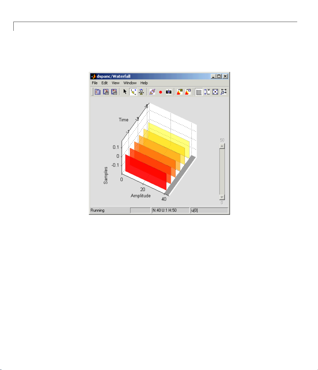
4 The d
spanc/Waterfall scope window displays the behavior of the adaptive
er coefficients. The following figure shows the scope window when the
filt
lation begins. Each plot represents the values of the filter coefficients
simu
normalized LMS adaptive filter. In the figure, you can see that they
of a
initialized to zero. Also, the color of the plots fades from red to yellow.
are
2-3
2 Concepts,Terminology,andFeatureOverview
The current filter coefficients are plotted in red. The other plots represent
the filter coefficients at previous simulation times.
2-4
Thenextfigureshowsthedspanc/Waterfall scope window when the filter
coefficients have reached their steady state.

Sample Model and Block Libraries
5 To speed up or slow down the rate of filter adaption, double-click the switch
attached to the blocks labeled Fast Adapt and Slow Adapt. When you
connect the switch to the block labeled Fast Adapt, the filter coefficients
reach steady state in a shorter time. To hear the difference in the filtered
signals, run the demo using both the fast adapt and the slow adapt rates.
Listen to the filtered signal produced by each.
The “A daptive Filters” se ction of the Signal Processing Blockset User’s Guide
contains more information o n the Acoustic Noise Canceler demo.
Signal Processing Blockset Blocks
The Signal Processing Blockset produ ct organizes a collection of blocks
within nested libraries. These libraries are specifically for digital signal
processing applications. They include blocks for o perations su ch as multirate
and adaptive filtering, matrix manipulation, linear algebra, statistics, and
time-frequency transforms. You can locate these blocks using the main Signal
Processing Blockset library or the Simulink Library Browser:
2-5
2 Concepts,Terminology,andFeatureOverview
• “Accessing Blocks Directly” on page 2-6
• “Accessing Blocks with the Library Browser” on page 2-8
Accessing Blocks Directly
You can access the main Signal P rocessing Blockset l ib rary from the MATLAB
command line. This procedure shows you how to open this library and locate
the source blocks:
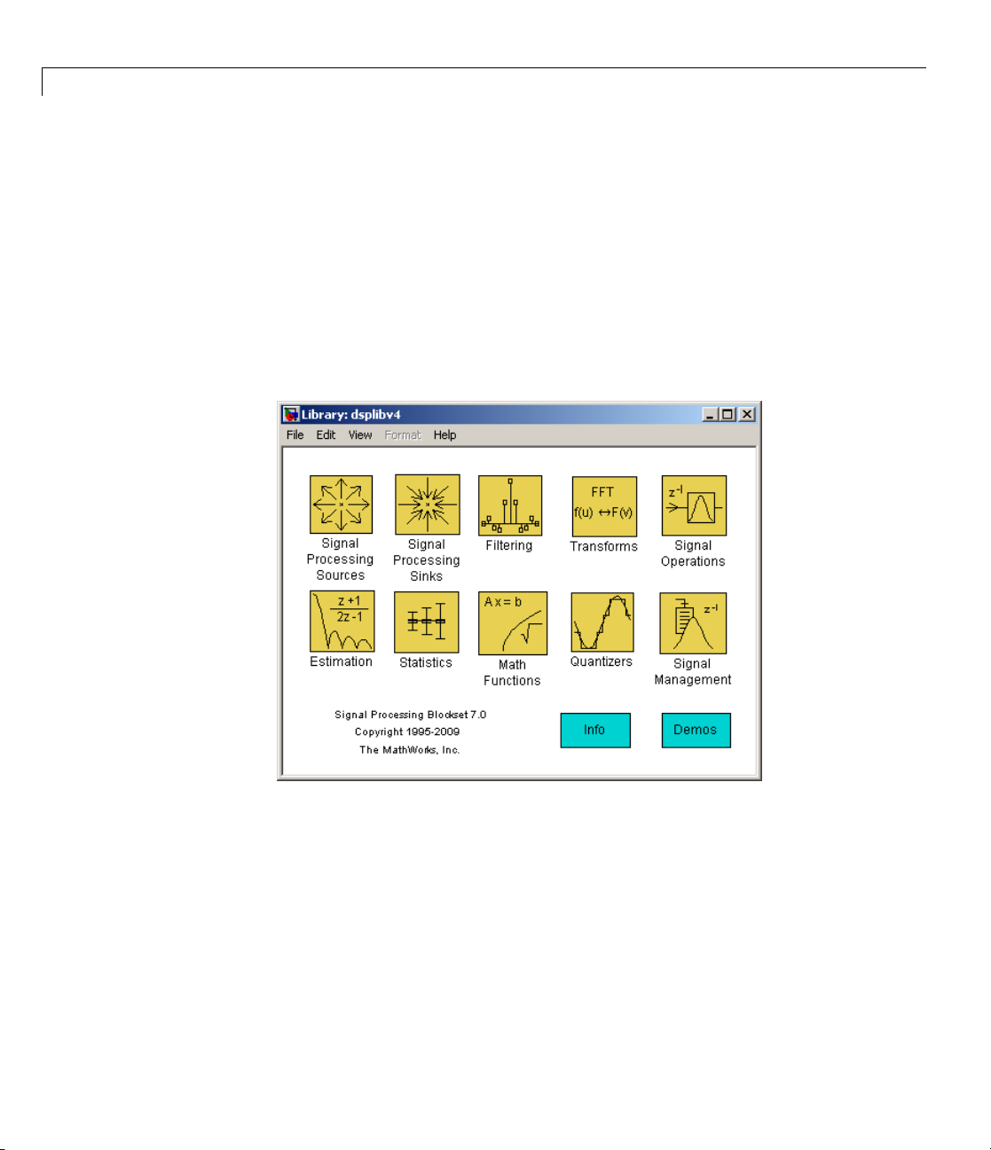
1 Open the library by typing ds plib at the MATLAB command prompt.
2-6
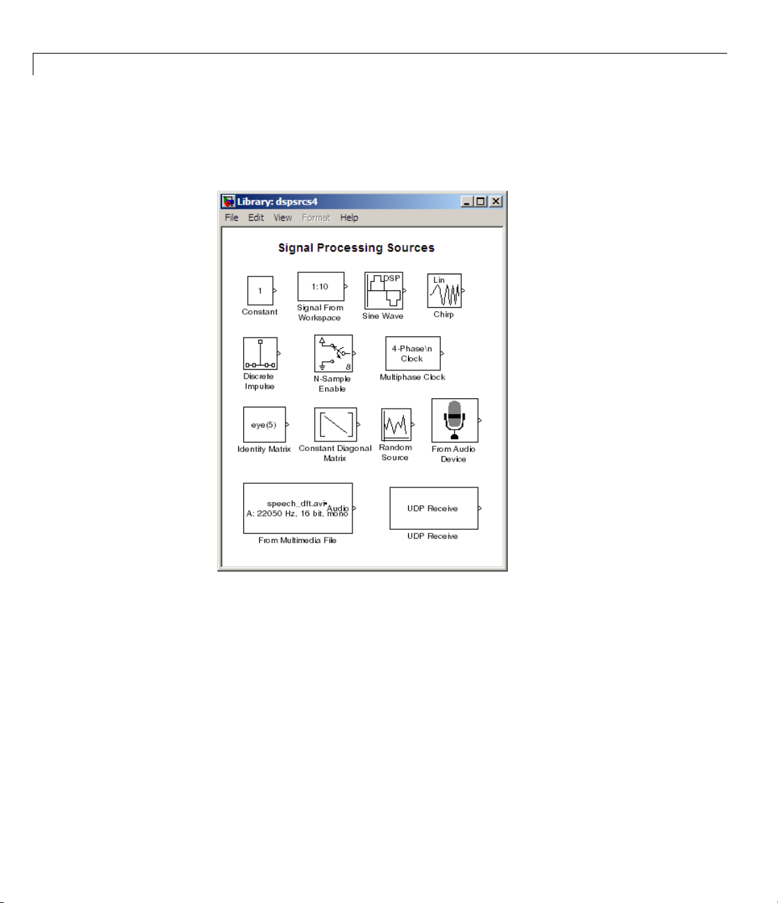
The Signal Processing Blockset libraries are
• Signal Processing Sources — Blocks that create discrete-time or
continuous-time signals or import these signals from the MATLAB
workspace
• Signal Processing Sinks — Blocks used to display data in a scope or s end
data to the MATLAB workspace
• Filtering — Blocks used to design digital, analog, adaptive, and
multirate filters

Sample Model and Block Libraries
• Transforms — Blocks that transform data into different domains
• Signal Operations — Blocks that perform operations such as convolution,
downsampling, upsampling, padding, and delaying the input
• Estimation — Blocks for linear prediction, parametric estimation, and
power spectrum estimation
• Statistics — Blocks that perform statistical operations such as
correlation, maximum, and mean
• Math Functions — Blocks used to perform mathematical operations,
matrix operations, and polynomial functions
• Quantizers — Blocks that create scalar and vector quantizers as well
as uniform encoders and decoders
• Signal Management — Blocks for buffering, selecting part of a signal,
modifying signal attributes, and edge detection
2 Double-click the Signal Processing Sources library. The library displays
the blocks it contains. You can use the blocks in this library to create
discrete-time or continuous-time signals.
2-7

2 Concepts,Terminology,andFeatureOverview
2-8
3 Drag any block into a model, double-click the block, and click Help to learn
more about the block functionality.
Acces
Starting the Simulink product displays the Simulink Library Browser. To
start Simulink, type
to explore the Signal Processing Blockset product is to expand the Signal
Processing Blockset entry in the tree pane of this browser.
sing Blocks with the Library Browser
simulink at the MATLAB command line. One way

Sample Model and Block Libraries
2-9

2 Concepts,Terminology,andFeatureOverview
Key Blockset Concepts
In this section...
“Signals” on page 2-10
“Sample Time” on page 2-10
“State” on page 2-11
“Sample-Based Signals” on page 2-11
“Frame-Based Signals” on page 2-12
“Tunable Parameters” on page 2-14
Signals
Signals in the Simulink environment can be real or complex valued. You
can represe nt signals w ith data types such as single-precision floating point,
double-precision floating point, or fixed point. Signals can be either sample
based or frame based, and single channel or multichannel.
2-10
Sample Time
A discrete-time signal is a sequence of values that correspond to particular
instants in time. The time instants at which the signal is defined are the
signal sample times, and the associated signal values are the signal samples.
For a periodically sampled signal, the equal interval between any pair of
consecutivesampletimesisthesignalsampleperiod,T
is the reciprocal of the sample period. It represents the number of samples in
the signal per second:
1
F
=
s
T
s
Note In the block parameter dialog boxes, the term sample time refers to
the sample period of the signal T
.
s
.Thesamplerate,Fs,
s

State
Some Signal Proc
ablockdoesnoth
current input.
current input a
If a block has state, the output of the block depends on the
s well as past inputs and/or outputs.
Key Blockset Concepts
essing Blockset blocks have state and others do not. If
ave state, the block calculates its output using only the
Sample-Based
Asignalissa
time. To repr
matrix. Each
is the total
signal with
matrix elem
total numb
Consider t
mple based if it propagates through the model one sample at a
esent a single-channel sample-based signal, create a 1-by-1-by-T
matrix element represents one sample from the channel, and T
number o f samples in the channel. To represent a multichannel
M*N independent channels, create an M-by-N-by-T matrix. Each
ent represents one sample from a distinct channel, and T is the
erofsamplesineachchannel.
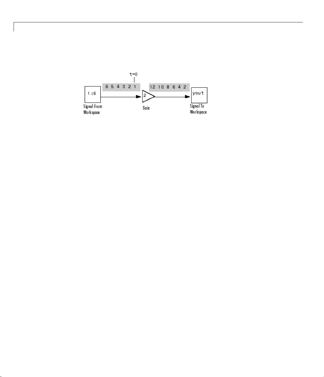
he following model.
Signals
The Signal From W orkspace block outputs a sample-based signal. The Gain
block multiplies all the samples of the signal by two. Then, the Signal To
Workspace b lock outputs the signal to the M ATLA B workspace in a variable
2-11
2 Concepts,Terminology,andFeatureOverview
called yout. The following figure is a symbolic representation of how the
single-channel, sample-based signal propagates through the model.
If you type yout at the MATLAB command prompt after you run the model,
you see, in part:
yout(:,:,1) =
2
yout(:,:,2) =
2-12
4
yout(:,:,3) =
6
Because yout represents a single-channel, sample-based signal, each sample
of the signal is a different page of the output matrix.
Frame-Based Signals
A signal is frame based if it propagates through a model one frame at a time.
A frame of data is a collection of sequential samples from a single channel o r
multiple channels. One frame of a single-channel signal is represented by an
M-by-1 column vector. One frame of a multichannel signal is represented by
anM-by-N matrix. Each matrix column is a different channel, and the number
of row s in the matrix is the number of samples in each frame.
You can typically specify whether a signal is frame based or sample based
using a source block from the Signal Processing Sources library. Most o ther

Key Blockset Concepts
signal processing blocks preserve the frame status of an input signal, but
some do not.
The process of propagating frames of data through a model is frame-based
processing. Because multiple samples can process at once, the computational
time of the model improves. “Working with S ignals” in the Signal Processing
Blockset User’s Guide contains more information about frame-based
processing.
Consider the following model.
To have the Signal From Workspace block output a frame-based signal, set
the Samples per frame parameter to
2 and run the model. The lines that
connect the blocks become double lines, indicating a frame-based signal; in
this example, there are two signals per frame.
The Gain block multiplies all the samples of this signal by two. Then, the
Signal To Workspace block outputs the signal to the MATLAB workspace
in the f orm of a variable called
yout. The following figure is a symbolic
representation of how the frame-based signal propagates through the model.
2-13

2 Concepts,Terminology,andFeatureOverview
If, after you ru
the following i
yout =
10
12
Because yo
is a column
workspac
Tunable P
There ar
To chang
open its
and the
Note Op
Simul
dialo
nclickOK. The simulation now uses the new parameter settings.
ink is paused, you can edit the parameter values. You must close the
g box to have the changes take effect and allow Simulink to continue.
nthemodel,youtype
s a portion of w hat you would s ee:
2
4
6
8
ut
represents a single-channel, frame-based signal, the output
vector. Once you export your signal values into the MATLAB
e, they are no longer grouped into frames.
arameters
e some parameters that you can change, or tune, during simulation.
e a tunable parameter during simulation, double-click the block to
dialog box, change any tunable parameters to the desired settings,
ening a dialog box for a source block causes Simulink to pause. While
yout at the M ATLA B command prom pt,
2-14
ule, parameters that specify numeric values are tunable. However, some
As a r
meters are not tunable, such as parameters that change the operational
para
of a block. For example, you cannot directly or indirectly change the
mode
lowing while a simulation is running:
fol
• Num
ber of block ports

Key Blockset Concepts
• Block sample rate
• Signal data type
For more information on tunable parameters, see the “Tunable Parameters”
section of the Simulink documentation.
2-15

2 Concepts,Terminology,andFeatureOverview
Signal Processing Blockset Product Features
In this section...
“Frame-Based Operations” on page 2-16
“Multirate Processing” on page 2-17
“Fixed-Point Support” on page 2-17
“Real-Time Code Generation” on page 2-18
“Adaptive and Mu ltira t e Filtering” on page 2-18
“Quantization” on page 2-18
“Statistical Operations” on page 2-19
“Linear Algebra” on page 2-1 9
“Parametric E stimation” on page 2-19
“Matrix Support” on page 2-20
“Data Type Support” on page 2-20
2-16
Frame-Based Operations
Most real-time signal processing systems optimize throughput rates
by processing data in “batch” or “frame-based” mode. By propagating
multisample frames instead of the individual signal samples, the signal
processing system can take advantage of the speed of signal processing
algorithm execution, while simultaneously reducing the demands placed on
the data acquisition (DAQ) hardware.
For an example of frame-based operations, open the LPC Analysis and
Synthesis of Speech demo by typing
prompt. To run this demo, from the Simulation menu, select Start.A
frame-based signal is used for computation throughout the model.
For more information about frame-based signals, see “Frame-Based Signals”
on page 2-12.
dsplpc at the MATLAB command

Signal Processing Blockset™ Product Features
Multirate Proce
Signal Proces si
that one port can
block. Multira
across the bloc
sublibrary, t
For more infor
Signal Proce
the Real-Tim
Fixed-Poin
Many Signal
you to desi
fixed-poi
• Signed tw
• Word size
• Word siz
• Overflo
nt arithmetic. Fixed-point support in the blockset includes:
code-ge
ng Blockset blocks support multirate processing. This means
have a different sample time than another port on the same
te processing is achieved by port-based sample time support
ks. Y ou can find multirate blocks in the Multirate Filters
he Signal Operations library, and the Buffers sublibrary.
mation, see “Inspecting Sample Rates and Frame Rates” in the
ssing Blockset User’s Guide and “Scheduling Considerations” in
eWorkshop
tSupport
Processing Blockset blocks have fixed-point support. This allows
gn discrete-time dynamic signal processing systems that use
o’s complement fixed-point data types
sfrom2to128bitsinsimulation
es from 2 to the size of a
neration target
w handling, scaling, and rounding methods
ssing
®
documentation.
long in the Real-Time Workshop ANSI C
• ANSI C c
proces
all all
autom
Simul
in har
ides built-in fixed-point operations that save time in simulation and
prov
ide automatically optimized code.
prov
ixed-point blocks, the Signal Processing Blockset and Real-Time
For f
kshop products produce optimized fixed-point code ready for execution
Wor
fixed-point processor. All the choices you make during simulation with
on a
blockset in terms of scaling, overflow handling, and rounding methods
the
e automatically optimized in the generated code, without the need for
ar
me-consuming and costly hand-optimized code.
ti
ode generation for deployment on a fixed-point embedded
sor, with the Real-Time Workshop product. The generated code uses
owed simulation data types supported by the embedded target, and
atically includes all necessary shift and scaling operations.
ating your fixed-point development choices before implementing them
dware saves time and money. Signal Processing Blockset software
2-17

2 Concepts,Terminology,andFeatureOverview
For more information on fixed-point sup p ort in the Signal Processing Blockset
product, see “Working with Fixed-Point Data” in the Signal Processing
Blockset User’s Guide.
Real-Time Code Generation
For all Signal Processing Blockset blocks, the Signal Processing Blockset and
Real-Time Workshop products produce optimized, compact, ANSI C code.
Chapter 5, “Code Generation” explains this process in more details.
Adaptive and Multirate Filtering
The Adaptive Filters and Multirate Filters sublibraries provide key tools
for the co ns truction of advanced signal processing systems. You can use
adaptive filter block parameters to tailor signal processing algorithms to
application-specific environments.
For an example of adaptive filtering, open the LMS Adaptive Equalization
demo by typing
is important in the field of communications. It involves estimating and
eliminating dispersion present in communication channels. In this demo, the
LMS Filter block models the dispersion of the system. The plot of the squared
error demonstrates the effectivenessofthisadaptivefilter.
lmsadeq at the MATLAB command prompt. Equalization
2-18
For more information on adaptive filters, see “Adaptive Filters” on page 4-9.
For more information on multirate filters, see “Multirate Filters” in the
Signal Processing Blockset User’s Guide.
Quantization
The process of quantization allows you to represent your input signal with
a finite number of values. This process helps you limit the bandwidth of
your transmitted signal. The Signal Processing Blockset product has a
number of blocks that can help you to design and implement scalar and
vector quantizers. In the main Signal Processing Blockset library, open the
Quantizers library to view the available blocks. See the block reference pages
for any of these blocks to find out more information about their functionality.

Signal Processing Blockset™ Product Features
For more inform ation about quantization, see “Analysis and Synthesis of
Speech” in the Signal Processing Blockset User’s Guide.
Statistical Operations
Use the blocks in the Statistics library for basic statistical analysis. These
blocks calculate measures of central tendency and spread such as mean,
standard deviation, and so on. They can also calculate the frequency
distribution of input values.
See “Statistics” in the Signal Processing Blockset User’s Guide for more
information.
Linear Algebra
The Matrices and Linear Algebra sublibrary provides Cholesky, LU, LDL,
and QR matrix factorization methods and equation solvers based on these
methods. It also provides blocks for common matrix operations.
See “Linear Algebra” in the Signal Processing Blockset User’s Guide for more
information.
Parametric Estimation
The Parametric Estimation sublibrary provides four blocks for modeling a
signal as the output of an AR system:
• Burg AR Estimator
• Covariance AR Estimator
• Modified Covariance AR Estim ator
• Yule-Wal ker AR Estimator
These blocks allow you to compute the AR s ystem parameters based on
forward error minimization, backward error minimization, or both.
In the Comparison of Spectral Analysis Techniques demo,
all-pole filter filters a Gaussian noise sample. Three different blocks, each
with its own method, estimate the spectrum of the IIR filter.
dspsacomp,anIIR
2-19

2 Concepts,Terminology,andFeatureOverview
Matrix Support
The Signal Processing Blockset product takes full advantage of the matrix
format of the Simulink environment. Some typical uses of matrices in signal
processing simulations are:
• General two-dimensional array
A matrix can be used in its traditional mathematical capacity, as a simple
structured array of numbers. The Matrices and Linear Algebra sublibrary
contains most of the blocks used for general matrix operations.
• Factored submatrices
A number of the matrix factorization blocks in the Matrix Facto r izations
sublibrary store the submatrix factors (such as low er and upper
submatrices) in a single compoun d matrix. See th e LDL Factorization and
LU Factorization b lo cks for examples.
• Multichannel frame-based signal
The standard format for m ultichannel frame-based signals is a matrix,
where each column represents a different channel. For example, a matrix
with three columns contains three channels of data. The number of rows in
the matrix is the number of samples in each frame.
2-20
The following sections of the Signal Processing Blockset User’s Guide provide
more information about working with matrices:
• “Creating Sample-Based Signals”
• “Creating Frame-Based Signals”
• “Creating Multichannel Sample-Based Signals”
• “Creating Multichannel Frame-Based Signals”
• “Deconstructing Multichannel Sample-Based S ig n als”
• “Deconstructing Multichannel Frame-Based Signals”
Data Type Support
All Signal Processing Blockset blocks support single- and double-precision
floating-point data types during both simulation and Real-Time Workshop C
code generation. Many blocks also support fixed-point and Boolean d ata types.

Signal Processing Blockset™ Product Features
To see which data types a particular block supports, refer to the “Supported
Data Types” section of the block reference page.
For information about data type support and code generation coverage for
all Signal Processing Blockset blocks, use the Signal Processing Blockset
Data Type Support Table. To access the table, select Help > Block
Support Table > Signal Processing Blockset or Help > Block Support
Table > All Tables from the Simulink model help menu.
You can also access the Signal Processing Blockset Data Type Support Table
by typing
showsignalblockdatatypetable at the MATLAB command line.
It is often necessary to convert between different data types when working
with Simulink models. The following table lists all data types supported by
2-21

2 Concepts,Terminology,andFeatureOverview
Signal Processing Blockset blocks and which function or block to use when
converting between data types.
Supported Data Types
Data Types
Supported by Signal
Processing Blockset
Blocks
Double-precision
floating point
Single-precision floating
point
Boolean
Integer (8-,16-, or
32-bits)
Unsigned integer
(8-,16-, or 32-bits)
Functions and Blocks for
Converting Data Types Comments
•
double
• Data Type Conversion block
single
•
• Data Type Conversion block
•
boolean
• Data Type Conversion block
int8, int16, int32
•
• Data Type Conversion block
•
uint8, uint16, uint32
• Data Type Conversion block
Simulink built-in data type
supported by all Signal
Processing Blockse t blocks
Simulink built-in data type
supported by all Signal
Processing Blockse t blocks
Simulink built-in data type.
Simulink built-in data type.
Simulink built-in data type.
Fixed-point data types
2-22
• Data Type Conversion block
• Simulink
num2fixpt function
®
Fixed Point™ product
• Functions and GUIs for designing
quantized filters with the Filter
Design Toolbox™ (compatible with
Filter Realization Wizard block)
To learn more a bout
fixed-point data types in th e
Signal Processing Blockset
product, see “Working with
Fixed-Point Data” in the
Signal Processing Blockset
User’s Guide.

Configuring the Sim uli nk®Environment for Signal Processing Models
Configuring the Simulink Environment for Signal
Processing Models
In this section...
“Using dspstartup.m” on page 2-23
“Settings in dspstartup.m” on page 2-24
Using dspstartup.m
The Signal Processing Blockset product provides a file, dspstartup.m,
that lets you automatically configure the Simulink environment for signal
processing simulation. We recommend these configuration parameters for
models that contain Signal Processing Blockset blocks. Because these blocks
calculate values directly rather than solving differential equations, you must
configure the Simulink solver to behave like a scheduler. The solver, while in
scheduler mode, uses a block sample time to determine when the code behind
each block executes. For example, if the sample time of a Sine Wave block
is
0.05, the solver executes the code behind this block and every other block
with this sample time once every 0.05 seconds.
Note When working with models that contains Signal Processing Blockset
blocks, use source blocks that enable you to specify their sample time. When
your source block does not have a Sample time parameter, you must add a
Zero-Order Hold block in your model and use it to specify the sample time.
For more information, see “Continuous-Time Source Blocks” in the Signal
Processing Blockset User’s Guide. The exception to this rule is the Constant
block, which can have a constant sample time. When it does, Simulink
executes this block and records the constant value once, which allows for
faster simulations and more compact generated code.
To use the dspstartup file to configure Simulink for signal processing
simulations, you can
• Type
dspstartup at the MATLAB command line. All new models have
settings customized for signal processing applications. Existing models
are not affected.
2-23

2 Concepts,Terminology,andFeatureOverview
• Place a call to dspstartup within the startup.m file. Thisisanefficient
way to use
you start Simulink. F or more information about performing automated
tasks a t startup, see the documentation for the
MATLAB Function Reference.
The
dspstartup file executes the following commands:
set_param(0, ...
dspstartup if you want these settings tobeineffecteverytime
'SingleTaskRateTransMsg','error', ...
'multiTaskRateTransMsg', 'error', ...
'Solver', 'fixedstepdiscrete', ...
'SolverMode', 'SingleTasking', ...
'StartTime', '0.0', ...
'StopTime', 'inf', ...
'FixedStep', 'auto', ...
'SaveTime', 'off', ...
'SaveOutput', 'off', ...
'AlgebraicLoopMsg', 'error', ...
'SignalLogging', 'off');
startup command in the
2-24
You can edit the dspstartup file to change any of these settings or to add
your own custom setting s. For complete information about these settings, see
“Model and Block Parameters” in the Simulink documentation.
Settings in dspstartup.m
A number of the settings in the dspstartup file are ch osen to improve the
performance of the simulation:
•
'Solver' is set to 'fixedstepdiscrete'.
This selects the fixed-step solver option instead of the Simulink default
variable-step solver. This mode enables code generation from the model
using the Real-Time Workshop product.
•
'Stop time' is set to 'Inf'.
The simulation runs until you manually stop it by selecting Stop from
the Simulation menu.
'SaveTime' is set to 'off'.
•

Configuring the Sim uli nk®Environment for Signal Processing Models
Simulink does not save the tout time-step vector to the workspace.
The time-step record is not usually ne eded for analyzing discrete-time
simulations, and disabling it saves a considerable amount of memory,
especially when the simulation runs for an extended time.
•
'SaveOutput' is set to 'off'.
Simulink Outport blocks in the top level of a model do not generate an
output (
yout)intheworkspace.
2-25

2 Concepts,Terminology,andFeatureOverview
2-26

Signal Processing Models
• “Creating a Block Diagram” on page 3-2
• “Setting the Model Parameters” on page 3-6
• “Running the Model” on page 3-9
• “Modifying Your Model” on page 3-12
3

3 Sign al Processing Models
Creating a Block Diagram
You can build signa l processing models using blocks from many different
Simulink and Signa l Processing Blockset libraries. In this section, you move
through the tasks needed to create a signal processing model that displays a
sine wave over time:
• Opening a new model
• Dragging blocks into the model
• Connecting the blocks
In subsequent procedures, you set the blo ck parameters and run the model.
Later in the book, you expand upon this model to create a system capable of
adaptive noise cancellation. You also use the Real-Time Workshop product to
generate code from this model:
1 Begin building y our model. Open the main Signal Processing Blockset
library by typing
dsplib at the MATLAB command prompt.
3-2

Creating a Block Diagram
2 Open a ne
Proces
sing Blockset library window.
w model by selecting File > New > Model in the Signal
3-3
3 Sign al Processing Models
3 Display the Signal Processing Blockset Sources sublibrary by
double-clicking the Signal Processing Sources icon in the main library
window.
3-4
4 Click-and-drag a Sine Wave block into your new model. The Sine Wave
block generates a sinusoidal signal.

Creating a Block Diagram
5 Add a Scope block from the Simulink Sinks library to your model.
6 Connect the two blocks by selecting the Sine Wave block, holding down the
Ctrl key, and then selecting the Scope block.
Now that you have created a model, you are ready to set your model
parameters.
3-5

3 Sign al Processing Models
Setting the Model Parameters
Once you have built your signal processing model, you can set your m odel
parameters. Nearly all blocks have an associated block parameters dialog
box. Double-click the block to display th is dialog box. Enter values into
this dialog box to ensure that your model accurately simulates the desired
behavior of your system.
Note Thesoftwareprovidespremademodels as starting points to each
procedure in this manual. To prev ent yourself from overwriting these models,
from the File menu, select Save as. Then, save your modified model in a
different folder.
1 If the model you created in “Creating a Block Diagram” on page 3-2 is not
open on your desktop, you can open an equivalent model by typing
doc_gstut1
3-6
at the MATLAB command prompt.
2 Open the Configuration Parameters dialog box by selecting
Simulation > Configuration Parameters from the model menu.
3 Set the
• Type:
• Solver: Discrete (no continuous states)
These are the recom mended Solver options for Signal Processing Blockset
models. For more information on recommended settings, see “Configuring
the Simulink Environment for Signal Processing Models” on page 2-23.
The C
following Solver options:
Fixed-step
onfiguration Parameters dialog box should now appear as follows:

Setting the Model Parameters
4 Click O
5 OpentheSineWavedialogboxbydouble-clickingtheSineWaveblock.
6 Set the block parameters as follows:
• Frequency (Hz) =
K to apply the change and close the dialog box.
0.5
• Sample time = 0.05
3-7

3 Sign al Processing Models
3-8
Note On Signal Processing Blockset blocks, the Sample time parameter
represents the sample period of the signal. The sample period is the
amount of time between each sample of the signal.
7 Click OK to apply the settings and close the dialog box. Now that you
have set your model parameters, you are ready to run your model and
view its behavior.

Running the Model
After you set the desired model parameters, you can run your model and view
its behavior. The Signal P rocessing Blockset product has many scope blocks
thatyoucanusetodisplayyourmodel output. In this example, you use a
Simulink Scope block to view your sinusoida l signal:
1 If the model you created in “Setting the Model Parameters” on page 3-6 is
notopenonyourdesktop,youcanopenanequivalentmodelbytyping
doc_gstut2
at the MATLAB command prompt.
2 Run the model by selecting Start from the Simulation menu.
Running the Model
3 Display th
Scope bloc
4 Autoscale the output to fit in the scope window by clicking .
e sinusoidal signal in the Scope window by double-clicking the
k.
3-9

3 Sign al Processing Models
You can achieve a m o re finely sampled output by decreasing the Sample
time parameter. For example, change the Sample time parameter in the
Sine Wave block to
Scope window should now look similar to the following figure.
0.005, run the model, and autoscale the output. The
3-10

Running the Model
5 Experiment with your model. Change the Frequency (Hz) and Sample
time parametersoftheSineWaveblock. The n, run your model to see
the effect. Now you are ready to add noise to your sinusoidal signal and
view its effect.
3-11

3 Sign al Processing Models
Modifying Your Model
A system’s input signal can contain noise that was introduced as the signal
traveled over a wire or through the air. You can incorporate noise into
the model of your system to simulate this real-world noise. Then, you can
experiment with ways to eliminate its effect at both low and high frequencies.
In this topic, you model a real-world signal by adding noise to your input
signal. In the next chapter, you u se a filter to convert this noise to low
frequency noise and another filter to eliminate this noise from your signal:
1 If the model you worked with in “Running the Model” on page 3-9 is not
open on your desktop, you can open an equivalent model by typing
doc_gstut2
at the MATLAB command prompt.
2 Add a Random Source block to your model from the Signal P rocessing
Sources library to represent the noise in your system. Set the block
parameters before you connect the blocks. Double-click the Random Source
block and set the block parameters as follows:
3-12
• Source type =
• Method = Ziggurat
• Mean = 0
• Variance = 1
• Repeatability = Specify seed
• Initial seed = [23341]
• Sample time = 0.05
Based on these parameters, the Random Source block produces Gaussian
random values using the
Initial seed parameters ensure that the block outputs the same signal
each time you run the model. The following figure shows the completed
Random Source dialog box.
Gaussian
Ziggurat method. The Repeatability and

Modifying Your Model
Opening this dialog box causes a running simulation to pause. While
simulation is paused, you can edit the parameter values. You mus t close the
dialog b ox to h av e the changes take effect and allow simulation to resume.
3 Add a Sum block to your model from the Simulink Math Operations library
to add rand om noise to your input signal.
3-13

3 Sign al Processing Models
4 Set the Sum block parameters. Open the Sum dialo g box by double-clicking
the Su m block. Change the List of signs parameter to ++| and click OK.
5 Set the Scope parameters. Open the Scope window by double-clicking
the Scope block. Open the Scope parametersdialogboxbyclickingthe
Parameters icon in the Scope window.
3-14
In the Scope parameters dialog box, set the Number of axes parameter
to
2 and click OK. Now, the Scope window has two plotting windows and
the Scope block has two input ports.

Modifying Your Model
6 Connect the output of the Sine Wave block and the output of the Random
Source block to the input of the Sum block. Then, connect the output of the
Sum block to the second input of the Scope block. When you are finished,
your model should look similar to the figure below.
7 Verify the parameters of your Sine Wave block. Open the Sine Wave dialog
box by double-clicking the Sine Wave block. Verify that the Frequency
(Hz) parameter is set to
0.05. Note that the value of the Sample time parameter of the Sine
0.5 and the Sample time parameter is set to
Wave block is the same as the value of the Sample time parameter of
the Random Source block.
8 Run
your model and view the results in the Scope window. The block
plays the original sinusoidal signal in the top axes and the signal with
dis
noise in the bottom axes.
the
3-15

3 Sign al Processing Models
Note You can change the signal labels in the Scope w indow by
right-clicking the axes and selecting Axes properties.IntheTitle text
box, enter your signal label.
3-16
You have now created and run a signal processing model that displays a
sinusoidal signal over time. During this process, you created a digital sine
waveandvieweditintheScopewindow. Youalsoaddednoisetoyour
sinusoidal signal and viewed its effect. InChapter4,“Filters”,youincrease
the complexity of your signal processing model by adding filters to eliminate
thepresenceofthisnoise.

Filters
• “Digital Filters” on page 4-2
• “Adaptive Filters” on page 4-9
4

4 Filters
Digital Filters
In this section...
“Designing a Digital Filter” o n page 4-2
“Adding a Digital Filter to Your Model” on page 4-6
Designing a Digital Filter
You can design lowpass, highpass, bandpass, and bandstop filters using either
the Digital Filter Design block or the Filter Realization Wizard. These blocks
are capable of calculating filter coefficients for various filter structures. In
Chapter 3, “Signal Processing Models”, you added white noise to a sine wave
and viewed the resulting signal on a scope. In this section, you use the Digital
Filter Design block to convert this white noise to low frequency noise so you
can simulate its effect on your system.
As a practical application, suppose a pilot is speaking into a microphone
within the cockpit of an airplane. The noise of the wind passing over the
fuselage is also reaching the microphone. A sensor is measuring the noise of
the wind on the outside of the plane. You want to estimate the wind noise
insidethecockpitandsubtractitfromtheinputtothemicrophonesothat
only the pilot’s voice is transmitted. In this chapter, you first learn how to
model the low frequency noise that is reaching the microphone. Later, you
learn how to remove this noise so that only the pilot’s voice is heard.
4-2
In this topic, you use a Digital Filter Design block to create low frequency
noise, which models the wind noise inside the cockpit:
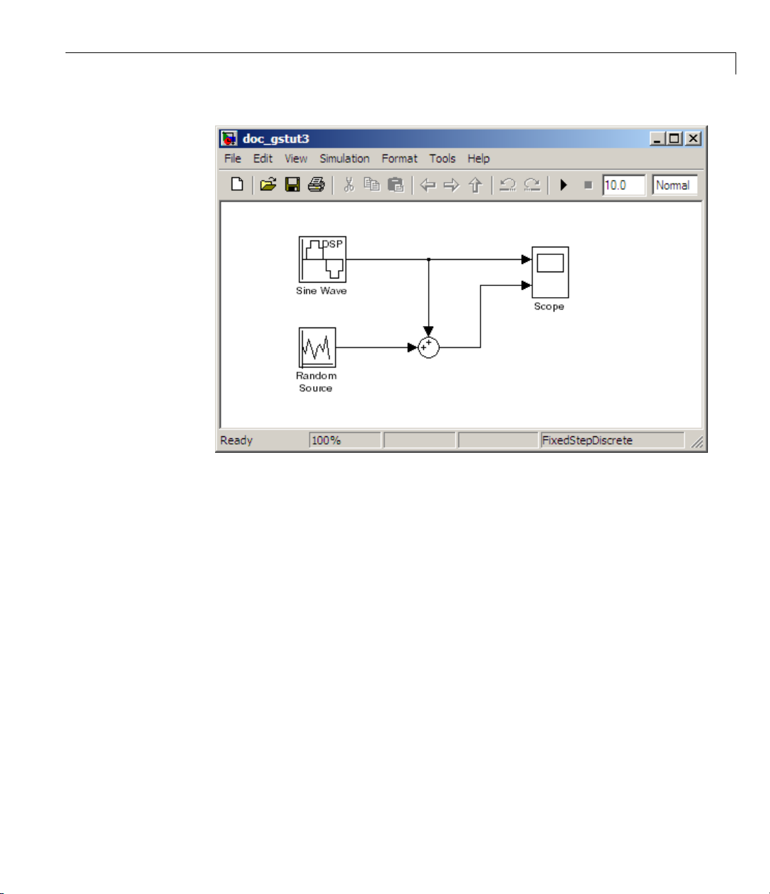
1 If the model you created in “Modifying Your Model” on page 3-12 is not
open on your desktop, you can open an equivalent model by typing
doc_gstut3
at the MATLAB command prompt. This model contains a Scope block that
displaystheoriginalsinewaveandthesinewavewithwhitenoiseadded.
Digital Filters
2 Open the Signal Processing Blockset library by typing dsplib at the
MATLAB command prompt.
3 Convert white noise to low frequency noise by introducing a Digital Filter
Design block into your model. In the airplane scenario, the air passing over
the fuselage creates white noise that is measured by a sensor. The Random
Source block models this noise. The fuselage of the airplane converts this
white noise to low frequency noise, a type of colored noise, which is h eard
inside the cockpit. This noise contains only certain frequencies and is more
difficult to eliminate. In this example, you model the low frequency noise
using a Digital Filter Design block. This block uses the functionality of the
Filter Design and Analysis Tool (FDATool) to design a filter.
le-click the Filtering library, and then double-click the Filter Designs
Doub
ibrary. Click-and-drag the Digital Filter Design block into your model.
subl
4-3

4 Filters
4-4
4 Set the Digital Filter Design block parameters to design a lowpass filter
and create low frequency noise. Open the block parameters dialog box by
double-clicking the block. Set the parameters as follows:
• Response Type =
• Design Method = FIR and, from the list, choose Window
• Filter Order = Specify order and enter 31
• Scale Passband —Cleared
• Window =
• Units = Normalized (0 to 1)
• wc = 0.5
Based on these parameters, the Digital Filter Design block designs a
lowpass FIR filter with 32 coefficients and a cutoff frequency of 0.5. The
block multiplies the time-domain response of your filter by a 32 sample
Hamming window.
Hamming
Lowpass

5 Click Design Filter at the bottom center of the dialog box to view the
magnitude response of your filter in the Magnitude R esponse pane. The
Digital Filter Design dialog box should now look similar to the following
figure.
Digital Filters
You have now designed a digital lowpass filter using the Digital Filter De sign
block.
You can experiment with the D igital Filter Design block in order to design a
filter of your own. For more information on the block functionality, see the
Digital Filter Design block reference page. For more information on the Filter
4-5

4 Filters
Design and Analysis Tool, see “FDATool: A Filter Design and Analysis GUI”
in the Signal Processing Toolbox documentation.
Adding a Digital Filter to Your Model
In this topic, you add the lowpass filter you designed in “Designing a Digital
Filter” on page 4-2 to your block diagram. Use this filter, which converts
white noise to colored noise, to simulate the low frequency wind noise inside
the cockpit:
1 If the model you created in “Designing a Digital Filter” on page 4-2 is not
open on your desktop, you can open an equivalent model by typing
doc_gstut4
at the MATLAB command prompt.
4-6

2 Incorporate the Digital Filter Design block into your block diagram by
placing it between the Random Source block and the Sum block.
Digital Filters
3 Run your model and view the results in the Scope window. This window
shows the original input signal and the signal with low frequency noise
added to it.
4-7

4 Filters
You have now built a digital filter and used it to model the presence of colored
noise in your signal. This is analogous to modeling the low frequency noise
reaching the microphone in the cockpit of the aircraft. Now that you have
added noise to your system, you can experiment with methods to eliminate it.
4-8

Adaptive Filters
In this section...
“Designing an Adaptive Filter” on page 4-9
“Adding the Adaptive Filter to Your Model” on page 4-14
“Viewing the Coefficients of Your Adaptive Filter” on page 4-19
Designing an Adaptive Filter
Adaptive filters track the dynamic nature of a system and allow you to
eliminate time-varying signals. The Signal Process ing Blockset libraries
contain blocks that implement least-mean-square (LMS), Block LMS, Fast
Block LMS, and recursive least s quares (RLS) adaptive filter algorithms.
These filters minimize the difference between the output signal and the
desired signal by altering their filter coefficients. Over time, the adaptive
filter’s output signal more closely approximates the signal you want to
reproduce.
Adaptive Filters
Inthistopic,youdesignanLMSadaptive filter to remove the low frequency
noise in your signal:
1 If the model you created in “Adding a Digital Filter to Your Model” on page
4-6 is not open on your des ktop, you can open an equivalent model by typing
doc_gstut5
at the MATLAB command prompt.
4-9

4 Filters
4-10
2 Open the Signal Processing Blockset library by typing dsplib at the
MATLAB command prompt.
3 Remove the low frequency noise from your signal by adding an LMS
Filter block to your system. In the airplane scenario, this is equivalent
to subtracting the wind noise inside the cockpit from the input to the
microphone. Double-click the Filtering sublibrary, and then double-click
the Adaptive Filters library. Add t h e LMS Filter block into your model.

Adaptive Filters
4 Set the LMS Filter block parameters to model the output of the Digital
Filter Design block. Open its dialog box by double-clicking the block. Set
the block parameters as follows:
• Algorithm =
Normalized LMS
• Filter length = 32
• Specify step size via = Dialog
• Step size (mu) = 0.1
• Leakage factor (0 to 1) = 1.0
• Initial value of filter weights = 0
4-11

4 Filters
• Clear the Adapt port check box.
• Reset port =
• Select the Output filter weights check box.
The LMS Filter dialog box should now look like the following figure:
None
4-12

Adaptive Filters
5 Click Apply.
4-13

4 Filters
Based on these parameters, the LMS Filter block computes the filter weights
using the normalized LMS equations. The filter order you specified is the
same as the filter order of the Digital Filter Design block. The Step size (mu)
parameter defines the granularity of the filter update steps. Because you set
the Leakage factor (0 to 1) parameter to
values depend on the filter’s initial conditions and all of the previous input
values. The initial valu e of the filter weights (coefficients) is zero. Since you
selected the Output filter weights check box, the Wts port appears on the
block. The block outputs the filter weights from this port.
Now that you have set the block parameters of the LMS Filter block, you can
incorporate this block into your block diagram.
1.0, the current filter coefficient
Adding the Adaptive Filter to Your Model
In this topic, you recover your original sinusoidal signal by incorporating the
adaptivefilteryoudesignedin“DesigninganAdaptiveFilter”onpage4-9
into your system. In the aircraft scenario, the adaptive filter models the low
frequency noise heard inside the cockpit. As a result, you can remove the
noise so that the pilot’s voice is the only input to the microphone:
4-14
1 If the model you created in “Designing an Adaptive Filter” on page 4-9 is
notopenonyourdesktop,youcanopenanequivalentmodelbytyping
doc_gstut6
at the MATLAB command prompt.

Adaptive Filters
2 Add a Sum block to your model to subtract the output of the adaptive filter
from the sinusoidal signal with low frequency noise. From the Simulink
Math Operations library, drag a Sum block into your model. Open the
Sum dialog box by double-clicking this block. Change the List of signs
parameter to |+- and then click OK.
3 Incorporate the LMS Filter block into your system.
a Connect the output of the Random Source block to the Input port of the
LMS Filter block. In the aircraft scenario, the random noise is the white
noise measured by the sensor on the outside of the airplane. The LMS
Filter block models the effect of the airplane’s fuselage on the noise.
b Connect the output of the Digital Filter De s ig n block to the De s ire d port
on the LMS Filter block. This is the signal you want the LMS block to
reproduce.
4-15

4 Filters
c Connect the output of the LM S Filter block to the negative port of the
Sum block you added in step 2.
d Connect the output of the first Sum block to the positive port of the
second Sum block. Your m odel should now look similar to the following
figure.
4-16
The positive input to the second Sum block is the sum of the input signal
and the low frequency noise, s(n)+y. The negative input to the second Sum
block is the LMS Filter block’s best estimation of the low frequency noise,

Adaptive Filters
y’. When you subtract the two signals, you are left with an approximation
of the input signal.
sn sn y y
() () ’=+−
approx
In this equation:
• s(n) is the input signal
sn
()
•
approx
is the approxim ation of the input signal
• y is the noise created by the Random Source block and the Digital Filter
Design block
• y’ is the LMS Filter block’s approximation of the noise
Because the LMS Filter block can only approximate the noise, there is still
a difference between the input signal and the approximation of the input
signal. In subsequent steps, you set up the Scope block so you can compare
the original sinusoidal signal with its approximation.
4 Add two additional inputs and axes totheScopeblock. OpentheScope
dialog box by do ubl e-click in g the Scope block. Click the Parameters
button. For the Number of axes parameter, enter
4. Close the dialog
box by clicking OK.
5 Label the new Scope axes. In the Scope window, right-click on the third
axes and select Axes properties. The Scope properties: axis 3 dialog box
opens. In the Title box, enter
Approximation of Input Si gnal.Close
the dialog box by clicking OK. Repeat this procedure for the fourth axes
and label it
6 Connect the output of the second Sum block to the third port of the Scope
Error.
block.
7 Connect the output of the Error port on the LMS Filter block to the fourth
port of the Scope block. Your mo de l should now look similar to the following
figure.
4-17

4 Filters
4-18
In this example, the output of the Error port is the difference between the
LMS filter’s desired signal and its output signal. Because the error is never
zero, the filter continues to modify the filter coefficients in order to better
approximate the low frequency noise. The better the approximation, the more
low frequency noise that can be removed from the sinusoidal signal. In the
next topic, “Viewing t he Coefficients of Your Adaptive Filter” on page 4-19,
you learn how to view the coefficients of your adaptive filter as they change
with time.

Adaptive Filters
Viewing the Coefficients of Your Adaptive Filter
The coefficients of an adaptive filter change with time in accordance with a
chosen algorithm. Once the algorithm optimizes the filter’s performance,
these filter coefficients reach their steady-state values. You can view the
variation of your coefficients, while the simulation is running, to see them
settle to their steady-state values. Then, you can determine whether you can
implement these values in your actual system:
1 If the model you created in “Adding the Adaptive Filter to Your Model” on
page4-14isnotopenonyourdesktop,youcanopenanequivalentmodel
by typing
doc_gstut7
at the MATLAB comm and prompt. Note that the Wts port of the adaptive
filter, which outputs the filter weights, still needs to be connected.
4-19

4 Filters
4-20
2 Open the Signal Processing Blockset library by typing dsplib at the
MATLAB command prompt.
3 View the filter coefficients using a Vector Scope block from the Signal
Processing Sinks library.
4 Open the Vector Scope dialog box by double-clicking the block. Set the
block parameters as follows:
a Click the Scope P roperties tab.

• Input domain = Time
• Time display span (number of frames) = 1
b Click the Display Properties tab.
• Select the following check boxes:
– Show grid
– Fram e number
– C ompact display
– Open scope at start of simulation
c Click the Axis Properties tab.
Adaptive Filters
• Minimum Y-limit =
-0.2
• Maximum Y-limit = 0.6
• Y-axis label = Filter Weights
d Click the Line Properties tab.
• Line visibilities =
on
• Line style = :
• Line markers =.
• Line colors = [0 0 1]
e Click OK.
5 Connect the Wts port of the LMS Filter block to the Vector Scope block.
4-21

4 Filters
4-22
6 Set the configuration parameters:
a Open the Configuration Parameters dialog box by selecting
Configuration Parameters from the Simulation menu, and navigate
to the Solver pa ne.
b Enter inf for the Stop time parameter.
c Choose Fixed-step from the Type list.
d Choose Discrete (no continuous states) from the Solver list.

Adaptive Filters
We recommend these configuration parameters for models that contain
Signal Processing Blockset blocks. Because these blocks calculate values
directly rather than solving d if ferential equations, you must configure the
Simulink Solver to behave like a scheduler. The Solver, while in scheduler
mode, uses a block’s sample time to determine when the code behind each
block is executed. For example, the sample time of the Sine Wave and
Random Source blocks in this model is
0.05. The Solver executes the code
behind these blocks, and every other block with this sample time, once
every 0.05 second.
Note When working with models that contain Signal Processing Blockset
blocks, use source blocks that enable you to specify their sample time. If
your source block does not have a Sample time parameter, you must add a
Zero-Order Hold block in your model and use it to specify the sample time.
For more information, see “Continuous-Time Source Blocks” in the Signal
Processing Blockset User’s Guide. The exception to this rule is the Constant
block, which can have a constant sample time. When it does, Simulink
executes this block and records the constant value once, which allows for
faster simulations and more compact generated code.
7 ClosethedialogboxbyclickingOK.
8 Open the Scope window by double-clicking the Scope block.
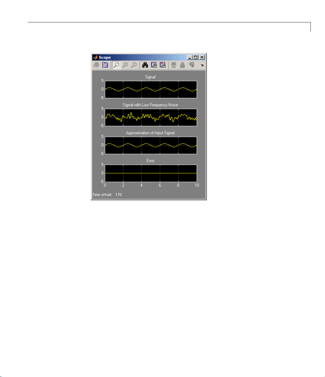
9 Run your model and view the behavior of your filter coefficients in the
Vector Scope window, which opens automatically when your simulation
starts. Over time, you see the filter coefficients change and approach their
steady-state values, shown below.
4-23

4 Filters
4-24
You can simultaneously view the behavior of the system in the Scope
window. Over time, you see the error decrease and the approximation of
the input signal more closely match the original sinusoidal input signal.
Adaptive Filters
You have
far, you
Design
LMS Fil
capabl
infor
Signa
Becau
sing
in yo
Simu
solv
the
In C
to g
now created a model capable of adaptive noise cancellation. So
have learned how to design a lowpass filter using the Digital Filter
block. You also learned how to create an adaptive filter using the
ter block. The Signal Proce ssing Blockset product has other blocks
e of designing and implementing digital and adaptive filters. For m ore
mation on the filtering capabilities of this product, see “Filters” in the
l Processing Blockset User’s Guide.
seallblocksinthismodelhavethesamesampletime,thismodelis
le rate and Simulink ran it in
SingleTasking solver mode. If the blocks
ur model have different sample times, your model is multirate and
link might run it in
MultiTasking solv er mode. For more information on
er mo de s, see “Recommended Settings for Discrete-Time Simulations” in
Signal Processing Blockset User’s Guide.
hapter 5, “Code Generation”, you use the Real-Time Workshop product
enerate code from your model.
4-25

4 Filters
4-26

Code Generation
• “Understanding Code Generation” on page 5-2
• “Generating Code” on page 5-4
5

5 Code Generation
Understanding Code Generation
In this section...
“CodeGenerationwiththeReal-TimeWorkshopProduct”onpage5-2
“Highly O ptimized Generated ANSI C Code” on page 5-3
Code Generation with the Real-Time Workshop Product
You can use the Signal Processing Blockset, Real-Time Workshop, and
Real-Time Workshop
code that you can use to implement your model for a practical application.
For instance, you can create an executable from your Simulink model to run
on a target chip.
This chapter introduces you to the basic concepts of code generation
using these tools. For more information on code generation, see “Building
Executables” in the Real-Time Workshop documentation.
®
Embedded Coder™ products together to generate
5-2
Shared Library Dependencies
For the blocks listed in the table be low, copy the shared library files from the
machine where the blockset software is installed to a folder on the system
path of the destination machine.
Block
To Multimedia File
From Multimedia File
udio Device
To A
From Audio Device
Depend
tommf
Sldir
from
Sld
libaudiodevice.dll
libportaudio.dll
libaudiodevice.dll
libportaudio.dll
ent library file
ile.dll
ectShow.dll
mmfile.dll
irectShow.dll

Understanding Code Generation
Highly Optimize
AllSignalProce
This C code is oft
following opti
• Function reus
common algori
functions are
core algorit
precompiled
generate sma
• Parameter r
many cases,
same value f
variable i
• Blocks hav
blocks, s
enable yo
optimiza
• Other op
reusabl
smaller
ssing Blockset blocks generate highly optimized ANSI C code.
en suitable for embedded applications, and includes the
mizations:
e(run-timelibraries)— The generated code reuses
thmic functions via calls to run-time functions. Run-time
highly optimized ANSI/ISO C functions that implement
hms such as FFT and convolution. Run-time functions are
into ANSI/ISO C run-time libraries, and enable the blocks to
ller, faster code that requires less m emory.
euse (Real-Time Workshop run-time parameters) —In
if there are multiple instances of a block that all have the
or a specific parameter, each block instance points to the same
n the generated code. This process reduces memory requirements.
e parameters that affect code optimization —Various
uch as the FFT and Sine Wave blocks, have parameters that
u to optimize the simulation for memory or for speed. These
tions also apply to code generation.
timizations — Use of contiguous input and output arrays,
e inputs, overwritable arrays, and inlined algorithms provide
generated C code that is more efficient at run time.
d Generated ANSI C Code
5-3

5 Code Generation
Generating Code
In this section...
“Setting Up the Build Folder” on page 5-4
“Setting Configuration Parameters” on page 5-5
“Generating C ode” on page 5-10
“Viewing the Generated Code” on page 5-11
Note You must hav e both the Signal Processing Blockset and Real-Time
Workshop products installed on your computer to complete this section’s
procedures.
Setting Up the Build Folder
First, you need to create a filter folder and put a local copy of your model in
it. The Real-Time Workshop software creates a build folder within this filter
folder during code generation. The build folder name is
derived from the nam e of the source model and the selected target. The build
folder contains generated source code and other files created during the build
process. This procedure assumes that yourfilterfolderresidesondriveD:
(PC) or your home folder (UNIX):
model_target_rtw,
5-4
1 Setupyourfilterfolderbytyping
!mkdir d:\filter_example
on a PC, or
!mkdir ~/filter_example
on UNIX.
The “!” character passes the command that follows it to the operating
system, which creates the folder.
kethisyourworkingfolderbytyping
2 Ma
cd d:\filter_example.

Generating Code
3 If the model you created in “Viewing the Coefficients of Your Adaptive
Filter” on page 4-19 is not open on your desktop, you can open an equivalent
model by typing
doc_gstut8
at the MATLAB command prompt.
4 Save this model as gstut8.mdl in your new working folder.
Setting Configuration Parameters
Before you can generate code, you must set several model parameters using
the Configuration Parameters dialog box. To learn how to configure your
model and Real-Time Workshop product settings so that your generated code
accurately reflects your system, see the following topics:
• “Selecting a Solver Algorithm” on page 5-5
• “Selecting a Target Configuration” on page 5-6
• “Controlling Other Co de Generation Options” on page 5-9
In these procedures, you continue to work with
gstut8.mdl,themodelyou
saved in your working folder in “Setting Up the Build Folder” on page 5-4.
Selecting a Solver Algorithm
Specify parameters that enable Simulink software to solve your model:
1 Open the Configuration Parameters dialog box for this model by selecting
Configuration Parameters from the Simulation menu.
2 In the Select pane, click Solver . Set the parameters as follows:
• Start Time =
• Stop Time = 60.0
• Type = Fixed-step
• Solver = Discrete (no continuous states)
• Fixed step size (fundamental sample time) = 0.01
0.0
5-5

5 Code Generation
• Tasking mode for periodic sample times = SingleTasking
3 Click Apply.
When you are finished setting the parameters, the Solver pane should look
similar to the following figure.
5-6
cting a Target Configuration
Sele
All Signal Processing Blockset blocks support the following code generation
targets:
• Generic Real-Time (GRT) target
• Embedded Real-Time (ERT) target

Generating Code
The MathWorks supplies the Generic Real-Time (GRT) target with the
Real-Time Workshop product. This target uses the real-time code format and
supports external mode communication. You can use this target as a starting
point when creating a custom rapid prototyping target, or for validating the
generated code on your workstation.
The MathWorks supplies the Embedded Real-Time (ERT) target
with the Real-Time W orkshop Embedded Coder product. This
target configuration generates mo de l code for execution on an
independent embedded real-time system. For more information, see
http://www.mathworks.com/products/rtwembedded/.
A target configuration consists of system target file, a template makefile, and
a
make command. In most situations, rather than specifying these parameters
individually, you use the ready-to-run generic real-time target configuration.
This GRT target is designed to build a stand-alone executable program that
runs on your workstation:
1 If you have not already done so, open the Configuration Parameters dialog
box. In the Select pane, click Real-Time Workshop.
5-7

5 Code Generation
5-8
2 Make su
select
an exec
3 Select a target configuration. If the System target file is not already
specified as
re that the Generate code only check box is not selected. If y ou
this check box, the Real-Time Workshop product does not generate
utable after it has created source code.
grt.tlc,opentheSystem target file browser dialog box by
clicking Browse next to the System target file box. The System target
file browser displays a list of all currently available target configurations.
When you select a target configuration, the appropriate system target file,
template makefile, and
From the list of available configurations, select
Target
and then click OK.
make command are automatically chosen.
Generic Real-Time

Generating Code
The Real-Time Workshop pane now displays the correct system target
file (
grt.tlc), make command (make_rtw). and template makefile
(
grt_default_tmf).
Controlling Other Code Generation Options
There are a number of additional options that you can set using the
Configuration Parameters dialog box:
1 If you have not already done so, open the Configuration Parameters dialog
box.
2 Prevent data from being logged to the MATLAB w orkspace . In the Select
pane, click Data Import/Export,andthencleartheTime and Output
check boxes. The se check boxes control whether or not the respective
variables are sent to the w orkspace.
3 Create a navigable summary of source files when the model is bui lt. In the
Select pane, expand Real-Time Workshop.ClickReport,andselectthe
Create Code Generation repo rt and Launch report automatically
check boxes.
4 Make blocks that were eliminated as a result of optimizations appear as
comments i n the generated code. In the Select pane, expand Real-Time
5-9

5 Code Generation
Workshop.ClickComments, and then select the Show eliminated
blocks check box.
5 View progress information during code generation. In the Select pane, click
Debug, and then select the Verbose build check box. When this option is
selected, the MATLAB Command Window displays progress information
during code generation. The compiler also reports its progress there.
6 Apply these settings and close this dialog box by clicking OK.
7 Save the model in your working folder. Your configuration parameters are
saved within the model file.
Once you have configured your model, you are ready to generate code.
Generating Code
After you set the configuration parameters, you can generate code from your
model. In this procedure, you continue to work with
you saved in your working folder in “Setting Configuration Parameters” on
page 5-5:
gstut8.mdl,themodel
5-10
1 Open the Configuration Parameters dialog box. In the Select pane, click
Real-Time Workshop.
2 To start the build process, click Build on the Real-Time Workshop pane.
A number of message s concerning code generation and compilation appear
in the MATLAB Command Window. The initial messages are
### Starting Real-Time Workshop build procedure for model: gstut8
### Generating code int o build folder:
d:\filter_example\gstut8_grt_rtw
The content of the succeeding messages depends on your compiler and
operating system. The final message is
### Successful completion of Real-Time Workshop build procedure for model: gstut8
3 Type dir at the MATLAB command prompt. The working folder now
contains a build folder,
gstut8_grt_rtw, which the Real-Time W orkshop
product created. The generated source files a re in this folder.
 Loading...