Mathworks ROBUST CONTROL TOOLBOX 3 user guide

Download

Robust Control Too

User’s Guide

Gary Balas Richard Chiang Andy Packard Michael Safonov

lbox™ 3

How to Contact The MathWorks

www.mathworks. comp.soft-sys.matlab Newsgroup www.mathworks.com/contact_TS.html T echnical Support

suggest@mathworks.com Product enhancement suggestions bugs@mathwo doc@mathworks.com Documentation error reports service@mathworks.com Order status, license renewals, passcodes info@mathwo

com

rks.com

Web

Bug reports

Sales, prici

ng, and general information

508-647-7000 (Phone)

508-647-7001 (Fax)

The MathWorks, Inc. 3 Apple Hill Drive Natick, MA 01760-2098

For contact information about worldwide offices, see the MathWorks Web site.

Robust Control Toolbox™ User’s Guide

The software described in this document is furnished under a license agreement. The software may be used or copied only under the terms of the license agreement. No part of this manual may be photocopied or reproduced in any form without prior written consent from The MathW orks, Inc.

FEDERAL ACQUISITION: This provision applies to all acquisitions of the Program and Documentation by, for, or through the federal government of the United States. By accepting delivery of the Program or Documentation, the government hereby agrees that this software or documentation qualifies as commercial computer software or commercial computer software documentation as such terms are used or defined in FAR 12.212, DFARS Part 227.72, and DFARS 252.227-7014. Accordingly, the terms and conditions of this Agreement and only those rights specified in this Agreement, shall pertain to and govern theuse,modification,reproduction,release,performance,display,anddisclosureoftheProgramand Documentation by the federal government (or other entity acquiring for or through the federal government) and shall supersede any conflicting contractual terms or conditions. If this License fails to meet the government’s needs or is inconsistent in any respect with federal procurement law, the government agrees to return the Program and Docu mentation, unused, to The MathWorks, Inc.

Trademarks

MATLAB and Simulink are registered trademarks of The MathWorks, Inc. See

www.mathworks.com/trademarks for a list of additional trademarks. Other product or brand

names may be trademarks or registered trademarks of their respective holders.

Patents

The MathWorks products are protected by one or more U.S. patents. Please see

www.mathworks.com/patents for more information.

Revision History

September 2005 First printing New for Version 3.0.2 (Release 14SP3) March 2006 Online only Revised for Version 3.1 (Release 2006a) September 2006 Online only Revised for Version 3.1.1 (Release 2006b) March 2007 Online only Revised for Version 3.2 (Release 2007a) September 2007 Online only Revised for Version 3.3 (Release 2007b) March 2008 Online only Revised for Version 3.3.1 (Release 2008a) October 2008 Online only Revised for Version 3.3.2 (Release 2008b) March 2009 Online only Revised for Version 3.3.3 (Release 2009a) September 2009 Online only Revised for Version 3.4 (Release 2009b) March 2010 Online only Revised for Version 3.4.1 (Release 2010a)

Building Uncertain Models

Introduction to Uncertain Atoms .................... 1-2

Uncertain Real Parameters Uncertain LTI Dynamics Atoms Complex Parameter Atoms ComplexMatrixAtoms Unstructured Uncertain Dynamic Systems

......................... 1-3

..................... 1-10

.......................... 1-13

............................. 1-15

............ 1-17

Contents

Uncertain Matrices

Creating Uncertain Matrices from Uncertain Atoms Accessing Properties of a umat Row and Column Referencing MatrixOperationonumatObjects Substituting for Uncertain Atoms

Uncertain State-Space Systems (uss)

Creating Uncertain Systems Properties of uss Objects Sampling Uncertain Systems Feedback Around an Uncertain Plant Interpreting Uncertainty in Discrete Time Lifting a ss to a uss Handling Delays in uss

Uncertain frd

Creating Uncertain Frequency Response Objects Properties of ufrd Objects Interpreting Uncertainty in Discrete Time Lifting an frd to a ufrd Handling Delays in ufrd

................................ 1-19

....................... 1-20

....................... 1-21

................... 1-22

.................... 1-23

................ 1-26

........................ 1-26

............................ 1-27

........................ 1-28

................. 1-29

............. 1-31

................................ 1-32

............................. 1-32

..................................... 1-35

........................... 1-35

............. 1-37

............................. 1-38

............................ 1-38

..... 1-19

........ 1-35

Basic Control System Toolbox and MATLAB

Interconnections

................................ 1-39

Simplifying Representation of U ncertain Objects ..... 1-40

Effect of the Autosimplify Property Direct Use of simplify

.............................. 1-43

................... 1-41

Sampling Uncertain Objects

Generating One Sample Generating Many Samples Sampling ultidyn Atoms

Substitution by usubs

Specifying the Substitution with Structures Nominal and Random Values

Array Management for Uncertain Objects

Referencing Arrays Creating Arrays with stack and cat Functions Creating Arrays by Assignment Binary Operations with Arrays Creating Arrays with usample Creating Arrays with usubs Creating Arrays with gridureal Creating Arrays with repmat Creating Arrays with repsys Using permute and ipermute

Decomposing Uncertain Objects (for Advanced

Users)

Normalizing Functions for Uncertain Atoms Properties of the Decomposition Syntax of lftdata Advanced Syntax of lftdata

.......................................... 1-63

.............................. 1-49

................................ 1-52

.................................. 1-65

........................ 1-45

............................ 1-45

.......................... 1-45

............................ 1-46

............ 1-50

........................ 1-51

............ 1-52

.......... 1-53

...................... 1-55

...................... 1-56

....................... 1-57

......................... 1-58

...................... 1-59

........................ 1-60

........................ 1-61

........................ 1-62

........... 1-63

...................... 1-64

.......................... 1-68

vi Contents

Generalized Robustness Analysis

Introduction to Generalized Robustness Analysis .... 2-2

Robust Stability Marg in

............................ 2-4

Robust Performance Margin ........................ 2-5

Worst-Case Gain Measure

.......................... 2-6

Introduction to Linear Matrix Inequalities

Linear Matrix Inequalities ......................... 3-2

LMI Features

LMIs and LMI Problems

Three Generic LMI Problems

Further Mathematical Background

Bibliography

..................................... 3-2

............................ 3-4

........................ 3-5

................. 3-10

...................................... 3-11

LMI Lab

Introduction ...................................... 4-2

Some Terminology Overview o f the LMI Lab

SpecifyingaSystemofLMIs

ASimpleExample Initializing the LMI System Specifying the LMI Variables Specifying Individual LMIs Specifying LMIs with the LMI Editor How It All Works

Querying the LMI System Description

lmiinfo

.......................................... 4-21

................................. 4-2

........................... 4-5

........................ 4-8

................................. 4-9

......................... 4-11

........................ 4-11

......................... 4-13

................. 4-16

.................................. 4-19

............... 4-21

vii

lminbr and matnbr ................................ 4-21

LMI Solvers

From Decision to Matrix Variables and Vice Versa

Validating Results

Modifying a System of LMIs

Deleting an LMI Deleting a Matrix Variable Instantiating a Matrix Variable

Advanced Topics

Structured Matrix Variables Complex-Valued LMIs Specifying c Feasibility Radius Well-Posedness Issues Semi-Definite B(x) in gevp Problems Efficiency and Complexity Issues Solving M + P

Bibliography

....................................... 4-22

................................. 4-29

........................ 4-30

.................................. 4-30

.......................... 4-30

...................... 4-31

.................................. 4-33

........................ 4-33

............................. 4-35

xObjectivesformincx ................... 4-38

................................. 4-40

............................. 4-40

.................. 4-42

..................... 4-42

XQ + QTXTP<0 ...................... 4-43

...................................... 4-45

... 4-28

viii Contents

Analyzing Uncertainty Effects in Simulink

Overview ......................................... 5-2

Robust Control Toolbox Block Library

Specifying Uncertainty Using Uncertain State Space

Blocks

How to Specify Uncertainty i n Uncertain State Space

Next Steps

.......................................... 5-5

Blocks

........................................ 5-5

....................................... 5-7

.............. 5-4

Simulating Uncertainty Effects ..................... 5-8

How to Simulate Effects of Uncertainty How to Vary Uncertainty Values

Computing Uncertain State-Space Models from

Simulink Models

Ways to Compute Uncertain State-Space Models from

Simulink Models

Working with Models Conta in in g Uncertain State Space

Blocks

Working with Models Contain ing Core Simulink or Custom

Blocks

Next Steps

........................................ 5-19

........................................ 5-20

....................................... 5-25

................................ 5-19

..................... 5-8

............... 5-8

Analyzing Stability Margins

Using the loopmargin Command How Stability Margin Analysis Using Loopmargin Differs

Between Simulink and LTI Mode ls How to Analyze Stability Marg in of Si mulink Models Example — Computing Stability Margins of a Simulink

Model

......................................... 5-28

........................ 5-26

..................... 5-26

................. 5-26

Examples

Building Uncertain Models ......................... A-2

The LMI Lab

Analyzing U ncertainty Effects in Simulink

...................................... A-2

........... A-2

.... 5-27

x Contents

Building Uncertain Models

• “Introduction to Uncertain Atoms” on page 1-2

• “Uncertain Matrices” on page 1-19

• “Uncertain State-Space Systems (uss)” on page 1-26

• “Uncertain frd” on page 1-35

• “Basic Control System Toolbox and MATLAB Interconnections” on page

1-39

• “Simplifying Representation of Uncertain Objects” on page 1-40

• “Sampling Uncertain Objects” on page 1-45

• “Substitution by usubs” on page 1-49

• “A rray Management for Uncertain Objects” on page 1-52

• “D eco m po sing Uncertain Objects (for Advanced Users)” on page 1-63

1 Building Uncertain Models

Introduction to Uncertain Atoms

Uncertain atoms are the building blocks used to form uncertain matrix objects and uncertain system objects. There are 5 classes of uncertain atom s:

Function Description

ureal

ultidyn

ucomplex

ucomplexm

udyn

Uncertain real parameter

Uncertain, linear, time-invariant dynamics

Uncertain c

omplex parameter

Uncertain complex matrix

Uncertain dynamic system

All of th and set m System T instan

set(b,

Functi proper

For

Fo wi mo

e atoms have properties, which are accessed through

ethods. This

oolbox™ and MATLAB

ce,

get(a,'PropertyName') isthesameasa.PropertyName,and

'PropertyName',Value)

get and set interface mimics the Control

Handle Graphics®behavior. For

is the sam e as b.PropertyName = value. onality also includes tab-completion and case-insensitive, partial name ty matching.

eal

, ucomplex and ucomplexm atoms, the syntax is

p1 = ureal(name, NominalValue, Prop1, val1, Prop2, val2,...); p2 = ucomplex(name, NominalValue, Prop1, val1, Prop2, val2,...); p3 = ucomplexm(name, NominalValue, Prop1, val1, Prop2, val2,...);

ultidyn and udyn,theNominalValue is fixed, so the syntax is

p4 = ultidyn(name, ioSize, Prop1, val1, Prop2, val2,...); p5 = udyn(name, ioSize, Prop1, val1, Prop2, val2,...);

ureal, ultidyn, ucomplex and ucomplexm atoms, the command usample

ll generate a random instance (i.e., not uncertain) of the atom, within its

deled range. For example,

usample(p1)

get

1-2

Introduction to Uncertain Atoms

creates a random instance of the uncertain real parameter p1.Withan integer argument, whole array s of in stances can be created. For instance

usample(p4,100)

generates an array of 100 instances of the ultidyn object p4.See“Sampling Uncertain Objects” on page 1-45 to learn more about

usample.

Uncertain Real Parameters

An uncertain real parameter is used to represent a real number whose value is uncertain. Uncertain real parameters have a name (the and a nominal value (the (

PlusMinus, Range, Percentage) describe the uncertainty in parameter

NominalValue property). Several other properties

values.

Name property),

All properties of a

ureal can be accessed through get and set. The properties

are:

Properties Meaning Class

Name

NominalValue

Mode

Internal name

Nominal value of atom

Signifies whi ch description (from

'PlusMinus', 'Range', 'Percentage')

char

double

char

of uncertainty is invariant when

NominalValue is ch an ged

PlusMinus

Range

Percentage

Additive variation

Numerical range

Additive variation (% of absolute value of

scalar or 1x2 double

1x2 double

scalar or 1x2 double

nominal)

AutoSimplify

'off' | {'basic'} |'full'

char

The properties Range, Percentage an d PlusMinus are all automatically synchronized. If the nominal value is 0, then the

Mode cannot be

1-3

1 Building Uncertain Models

Percentage.TheMode property controls what aspect of the uncertainty

remains unchanged when

NominalValue is changed. Assigning to any of

Range/Percentage/PlusMinus changes the value, but does not change the

mode.

The

AutoSimplify property controls how expressions involving the real

parameter are simplified. Its default value is

'basic',whichmeans

elementary methods of sim pl if ication are applied as operations are completed. Other values for

'full' (model-reduction-like techniques are applied). See “Simplifying

AutoSimplify are 'off' (no simplification performed) and

Representation of Uncertain Objects” on page 1-40 to learn more about the

AutoSimplify property and the command simplify.

If no property/value pairs are specified, default values are used. The default

Mode is PlusMinus,andthedefaultvalueofPlusMinus is [-1 1].Some

examples are shown below. In many cases, the full property name is not specified, taking advantage of the case-insensitive, p artial name property matching.

1-4

Create an uncertain real parameter, nominal value 3, with default values for all uns pecified properties (including plus/minus variability of 1). View the properties and their values, and note that the

Range and Percentage

descriptions of variability are automatically ma intained.

a = ureal('a',3)

Uncertain Real Parameter: Name a, NominalValue 3, variability = [-1 1]

get(a)

Name: 'a'

NominalValue: 3

Mode: 'PlusMinus'

Range: [2 4]

PlusMinus: [-1 1]

Percentage: [-33.3333 33.3333]

AutoSimplify: 'basic'

Create an uncertain real parameter, nominal value 2, with 20% variability. Again, view the properties, and note that the

Range and PlusMinus

descriptions of variability are automatically ma intained.

b = ureal('b',2,'percentage',20)

Introduction to Uncertain Atoms

Uncertain Real Parameter: Name b, NominalValue 2, variability = [-20 20]%

get(b)

Name: 'b'

NominalValue: 2

Mode: 'Percentage'

Range: [1.6000 2.4000]

PlusMinus: [-0.4000 0.4000]

Percentage: [-20.0000 20.0000]

AutoSimplify: 'basic'

Change the range of the parameter. All descriptions of variability are automatically updated, while the nominal value remains fixed. Although the change in variability was accomplished by specifying the unaffected, and remains

b.Range = [1.9 2.3]; get(b)

Name: 'b'

NominalValue: 2

Mode: 'Percentage'

Range: [1.9000 2.3000]

PlusMinus: [-0.1000 0.3000]

Percentage: [-5.0000 15.0000]

AutoSimplify: 'basic'

Percentage.

Range,theMode is

As mentioned, the Mode property signifies what aspect of the uncertainty remains unchanged when parameter is in

Percentage mode, then the Range and PlusMinus properties

are determined from the

NominalValue preserves the Percentage property, and automatically updates

the

Range and PlusMinus properties.

b.NominalValue = 2.2; get(b)

Name: 'b'

NominalValue: 2.2000

Mode: 'Percentage'

Range: [2.0900 2.5300]

PlusMinus: [-0.1100 0.3300]

Percentage: [-5.0000 15.0000]

NominalValue is modified. Hence, if a real

Percentage property and NominalValue. Changing

1-5

1 Building Uncertain Models

AutoSimplify: 'basic'

Create an uncertain parameter with an unsymmetric variation about its nominal value.

c = ureal('c',-5,'per',[-20 30]); get(c)

Name: 'c'

NominalValue: -5

Mode: 'Percentage'

Range: [-6 -3.5000]

PlusMinus: [-1 1.5000]

Percentage: [-20 30]

AutoSimplify: 'basic'

Create an uncertain parameter, specifying variability with Percentage,but force the

d = ureal('d',-1,'mode','range','perc',[-40 60]); get(d)

Mode to be Range.

Name: 'd'

NominalValue: -1

Mode: 'Range'

Range: [-1.4000 -0.4000]

PlusMinus: [-0.4000 0.6000]

Percentage: [-40.0000 60]

AutoSimplify: 'basic'

1-6

Finally, create an uncertain real parameter, and set the AutoSimplify property to 'full'.

e = ureal('e',10,'plusminus',[-23],'mode','perce',...

'autosimplify','full')

Uncertain Real Parameter: Name e, NominalValue 10, variability = [-20 30]%

get(e)

Name: 'e'

NominalValue: 10

Mode: 'Percentage'

Range: [8 13]

PlusMinus: [-2 3]

Introduction to Uncertain Atoms

Percentage: [-20 30]

AutoSimplify: 'full'

Specifying conflicting values for Range/Percentage/PlusMinus in a multiple property/value property is used. This last occurrence also determines the

Mode is explicitly specified, in which ca se that is used, regardless of the

set is not an error. In this case, the last (in list) specified

Mode, unless

property/value pairs ordering.

f = ureal('f',3,'plusminus',[-2 1],'perce',40)

Uncertain Real Parameter: Name f, NominalValue 3, variability = [-40 40]%

g = ureal('g',2,'plusminus',[-2 1],'mode','range','perce',40)

Uncertain Real Parameter: Name g, NominalValue 2, Range [1.2 2.8]

g.Mode

ans =

Range

Create an uncertain real parameter, use usample to generate 1000 instances (resulting in a 1-by-1-by-1000 array), reshape the array, and plot a histogram, with 20 bins (within the range of 2 to 4).

h = ureal('h',3); hsample = usample(h,1000); hist(reshape(hsample,[1000 1]),20);

1-7

1 Building Uncertain Models

Make the range unsymmetric about the nominal value, and repeat the sampling, and histogram plot (with 40 bins over the range of 2-to-6)

1-8

h.Range = [2 6]; hsample = usample(h,1000); hist(reshape(hsample,[1000 1]),40);

Introduction to Uncertain Atoms

Note that the distribution is skewed. However, the number of samples less than the nominal value and the number of samples greater than the nominal value is equal (on average). Verify this.

length(find(hsample(:)<h.NominalValue)) ans =

509 length(find(hsample(:)>h.NominalValue)) ans =

491

The distribution used in usample is uniform in the normalized description of the uncertain real parameter. See “Decomposing Uncertain Objects (for Advanced Users)” on page 1-63 to learn more about the normalized description.

Thereisnonotionofanempty

ureal, by itself, creates an unnamed atom, with default property values. The

given name is

get(ureal)

'UNNAMED'. This can be observed with get and set.

Name: 'UNNAMED'

ureal (oranyotheratom,forthatmatter).

1-9

1 Building Uncertain Models

NominalValue: 0

Mode: 'PlusMinus'

Range: [-1 1]

PlusMinus: [-1 1]

Percentage: [-Inf Inf]

AutoSimplify: 'basic'

set(ureal)

Name: 'String'

NominalValue: '1x1 real DOUBLE'

Mode: 'Range | PlusMinus'

Range: '1x2 DOUBLE'

PlusMinus: '1x2 or scalar DOUBLE'

Percentage: 'Not settable since Nominal==0'

AutoSimplify: '['off' | 'basic' | 'full']'

Uncertain LTI Dynamics Atoms

Uncertain linear, time-invariant objects, ultidyn, are used to represent unknown linear, time-invariant dynamic objects, whose only known attributes are bounds on their frequency response. Uncertain linear, time-invariant objects have an internal name (the specifying their size (number of outputs and number of inputs).

Name property), and are created by

1-10

The property frequency response are related to gain or phase. The property

'GainBounded' or 'PositiveReal'. The default value is 'GainBounded'.

The property

Type specifies whether the known attributes about the

Type may be

Bound is a single number, which along with Type, completely

specifies what is known about the uncertain frequency response. S pecifically, if Δ is an

ultidyn atom, and if γ denotes the value of the Bound property, then

the atom represents the set of all stable, linear, time-invariant systems whose frequency response satisfies certain conditions:

Type is 'GainBounded', for all frequencies. When Type is

'GainBounded', the default value for Bound (i.e., γ)is1. TheNominalValue

of Δ is always the 0-matrix.

Type is 'PositiveReal', Δ(ω)+Δ

'PositiveReal', the default value for Bound (i.e., γ)is0.TheNominalValue

(ω)≥2·γ for all frequencies. When Type is

is always (γ+1+2|γ|)I.

Introduction to Uncertain Atoms

All properties of a ultidyn are can be accessed with get and set (although the

NominalValue is determined from Type and Bound, and not accessible

with

set). The properties are

Properties Meaning Class

Name

NominalValue

Type

Bound

SampleStateDim

Internal Name

Nominal value of atom

'GainBounded' |'PositiveReal'

Norm bound or minimum real

State-space dimension of random

char

See above

char

scalar double

samples of this uncertain element

AutoSimplify

'off' | {'basic'} |'full'

char

The SampleStateDim property specifies the state dimension of random samples of the atom wh en using

AutoSimplify property serves the same function as in the uncertain real

usample. The default value is 1. The

parameter.

You can create a 2-by-3 gain-bounded uncertain linear dynamics atom. Verify its size, and check the properties.

f = ultidyn('f',[2 3]); size(f) ans =

get(f)

Name: 'f'

NominalValue: [2x3 double]

Type: 'GainBounded'

Bound: 1

SampleStateDim: 1

AutoSimplify: 'basic'

You can create a 1-by-1 (scalar) positive-real uncertain linear dynamics atom, whose frequency response always has real part greater than -0.5. Set the

SampleStateDim property to 5. View the properties, and plot a Nyquist plot

of 30 instances of the atom.

1-11

1 Building Uncertain Models

g = ultidyn('g',[1 1],'type','positivereal','bound',-0.5); g.SampleStateDim = 5; get(g)

Name: 'g'

NominalValue: 1.5000

Type: 'PositiveReal'

Bound: -0.5000

SampleStateDim: 5

AutoSimplify: 'basic' nyquist(usample(g,30)) xlim([-2 10]) ylim([-6 6]);

1-12

Time-Domain of ultidyn Atoms

ts ow n, every

On i

h uncertain behavior, quantified by bounds (gain or real-part) on its

wit

quency response. To see this, create a

fre

everal random samples of the atom.

of s

ultidyn atom is interpreted as a continuous-time, system

ultidyn,andviewthesampletime

Introduction to Uncertain Atoms

h = ultidyn('h',[1 1]); get(usample(h),'Ts') ans =

0 get(usample(h),'Ts') ans =

However, when a ultidyn atom is an uncertain element of an uncertain state space model (

uss), then the time-domain characteristic of the atom is

determined from the time-domain characteristic of the system. The bounds (gain-bounded or positivity) apply to the frequency-response of the atom. This is explained and demonstrated in “Interpreting Uncertainty in Discrete Time” on page 1-31.

Complex Parameter Atoms

The ucomplex atom represents an uncertain complex n um ber, whose value lies in a disc, centered at property. The size of the disc can also be specified by Percentage,which means the radius is derived from the absolute value of the properties of

ucomplex objects a re

NominalValue, with radius specified by the Radius

NominalValue.The

Properties Meaning Class

Name

NominalValue

Mode

Radius

Percentage

AutoSimplify

Internal Name

Nominal v alue of atom

'Range' | 'Percentage'

Radius of disk

Additive variation (percent of

Radius)

'off' | {'basic'} | 'full'

char

double

char

double

char

The simplest construction requires only a nam e and nominal value. The default

Mode is Radius, and the default radius is 1.

1-13

1 Building Uncertain Models

a = ucomplex('a',2-j) Uncertain Complex Parameter: Name a, NominalValue 2-1i, Radius 1 get(a)

Name: 'a'

NominalValue: 2.0000- 1.0000i

Mode: 'Radius'

Radius: 1

Percentage: 44.7214

AutoSimplify: 'basic'

set(a)

Name: 'String'

NominalValue: '1x1 DOUBLE'

Mode: 'Radius | Percentage'

Radius: 'scalar DOUBLE'

Percentage: 'scalar DOUBLE'

AutoSimplify: '['off' | 'basic' | 'full']'

Sample the uncertain complex parameter at 400 values, and plot in the complex plane. Clearly, the samples appear to be from a disc of radius 1, centeredinthecomplexplaneatthevalue2-j.

1-14

asample = usample(a,400); plot(asample(:),'o'); xlim([0 4]); ylim([-3 1]);

Introduction to Uncertain Atoms

Complex Matrix Atoms

The uncertain complex matrix class, ucomplexm, represents the set of matrices given by the formula

where N,WL,WR are known matrices, and Δ is any complex matrix with

roperties of a

.Allp

The properties are

set.

Properties Meaning Class

Name

minalValue

Int

Nom

ucomplexm are c an be accessed with get and

ernal Name

inal value of atom

ft weight

char

uble

1-15

1 Building Uncertain Models

Properties Meaning Class

AutoSimplify

Right weight

'off' | {'basic'} | 'full'

double

char

The simplest construction requires only a nam e and nominal value. The defaultleftandrightweight matrices are identity.

You can create a 4-by-3

m = ucomplexm('m',[1 2 3;4 5 6;7 8 9;10 11 12]) Uncertain Complex Matrix: Name m, 4x3 get(m)

Name: 'm'

NominalValue: [4x3 double]

AutoSimplify: 'basic' m.NominalValue ans =

123 456 789

10 11 12 m.WL ans =

1000 0100 0010 0001

ucomplexm element, and view its properties.

WL: [4x4 double] WR: [3x3 double]

Sample the uncertain matrix, and compare to the nominal value. Note the element-by-element sizes of the difference are generally equal, indicative of the d efault (identity) weighting matrices that are in place.

1-16

abs(usample(m)-m.NominalValue) ans =

0.2948 0.1001 0.2867

0.3028 0.2384 0.2508

0.3376 0.1260 0.2506

Introduction to Uncertain Atoms

0.2200 0.3472 0.1657

Change the left and right weighting matrices, making the uncertainty larger as you move down the rows, and across the columns.

m.WL = diag([0.2 0.4 0.8 1.6]); m.WR = diag([0.1 1 4]);

Sample the uncertain matrix, and compare to the nominal value. Note the element-by-element sizes of the difference, and the general trend that the smallest differences are near the (1,1) element, and the largest differences are near the (4,3) element, which is completely expected by choice of the diagonal weighting matrices.

abs(usample(m)-m.NominalValue) ans =

0.0091 0.0860 0.2753

0.0057 0.1717 0.6413

0.0304 0.2756 1.4012

0.0527 0.4099 1.8335

Unstructured Uncertain Dynamic Systems

The unstructured uncertain dynamic system class, udyn,represents completely unknown multi va r iable, time-varying nonlinear systems.

For practical purposes, these uncertain elements represent noncommuting symbolic variables (placeholders). All algebraic operations, such as addition, subtraction, multiplication (i.e., cascade) operate properly, and substitution (with

usubs) is allowed. However, all of the analysis too ls (e.g., robuststab)

do not handle these types of uncertain elements. As such, these elements do not provide a significant amount of usability, and their role in the user’s guide is small.

You can create a

m = udyn('m',[2 3]) Uncertain Dynamic System: Name m, size 2x3 size(m) ans =

2-by-3 udyn element. Check its size, and properties.

1-17

1 Building Uncertain Models

get(m)

Name: 'm' NominalValue: [2x3 double] AutoSimplify: 'basic'

1-18

Uncertain Matrices

Uncertain m atrices (class umat) are built from double s, and uncertain atoms, using traditional MATLAB matrix building syntax. Uncertain matrices can be added, subtracted, multiplied, inverted, transposed, etc., resulting in uncertain matrices. The rows and columns of an uncertain matrix are referenced in the same manner that MATLAB references rows and columns of an array, using parenthesis, and integer indices. The uncertain matrix is the result obtained when all uncertain atoms are replaced with their own accessible through the within a

umat can be changed directly.

Uncertain Matrices

NominalValue of a

NominalValue. The uncertain atoms making u p a umat are

Uncertainty gateway, and the properties of each atom

Using atoms w ithin a

usubs, specific values may be substituted for any of the uncertain

umat.Thecommandusample generates a random sample of

the uncertain matrix, substituting random samples (within their ranges) for each of the uncertain atoms.

The command

wcnorm computes tight bounds on the worst-case (maximum

over the uncertain elements’ ranges) norm of the uncertain matrix.

Standard MATLAB numerical matrices (i.e.,

double) naturally can be viewed

as uncertain matrices without any uncertainty.

Creating Uncertain Matrices from Uncertain Atoms

You can create 2 uncertain real parameters, and then a 3-by-2 uncertain matrix using these uncertain atoms.

a = ureal('a',3); b = ureal('b',10,'pe',20); M = [-a 1/b;b a+1/b;1 3] UMAT: 3 Rows, 2 Columns

a: real, nominal = 3, variability = [-1 1], 2 occurrences b: real, nominal = 10, variability = [-20 20]%, 3 occurrences

ThesizeandclassofM are as expected

size(M) ans =

1-19

1 Building Uncertain Models

32 class(M) ans = umat

Accessing Properties of a umat

Use get to view the accessible properties of a umat.

get(M)

NominalValue: [3x2 double]

Uncertainty: [1x1 atomlist]

The NominalValue is a double, obtained by replacing all uncertain elements with their nominal values.

M.NominalValue ans =

-3.0000 0.1000

10.0000 3.1000

1.0000 3.0000

1-20

The Uncertainty property is a atomlist object, which is simply a gateway from the

umat to the uncertain atoms.

class(M.Uncertainty) ans = atomlist M.Uncertainty

a: [1x1 ureal] b: [1x1 ureal]

Direct access to the atoms is facilitated through Uncertainty.Checkthe

Range of the uncertain element named 'a' within M, then change it.

M.Uncertainty.a.Range ans =

24 M.Uncertainty.a.Range = [2.5 5]; M UMAT: 3 Rows, 2 Columns

Uncertain Matrices

a: real, nominal = 3, variability = [-0.5 2], 2 occurrences b: real, nominal = 10, variability = [-20 20]%, 3 occurrences

The change to the uncertain real parameter a only took place within M.Verify that the variable

a intheworkspaceisnolongerthesameasthevariablea

within M.

isequal(M.Uncertainty.a,a) ans =

Note that combining atoms which have a common internal name, but different properties leads to an error. For instance, subtracting the two atoms gives an error, not 0.

M.Uncertainty.a - a ??? Error using ==> ndlft.lftmask

Atoms named 'a' have different properties.

Row and Column Referencing

Standard Row/Column referencing is allowed. Note, however, that single-indexing is only allowed if the

Reconstruct

a = ureal('a',3); b = ureal('b',10,'pe',20); M = [-a 1/b;b a+1/b;1 3]; M.Uncertainty.a.Range = [2.5 5]; M(2:3,:) UMAT: 2 Rows, 2 Columns

a: real, nominal = 3, variability = [-0.5 2], 1 occurrence b: real, nominal = 10, variability = [-20 20]%, 2 occurrences

M (if need be), and make a 2-by-2 selection from M

Make a single column selection from M, and use single-index references to access elements of it.

h = M([2 1 2 3],2) UMAT: 4 Rows, 1 Columns

umat is a column or a row.

1-21

1 Building Uncertain Models

a: real, nominal = 3, variability = [-0.5 2], 1 occurrence

b: real, nominal = 10, variability = [-20 20]%, 1 occurrence h(2) UMAT: 1 Rows, 1 Columns

b: real, nominal = 10, variability = [-20 20]%, 1 occurrence h(3) UMAT: 1 Rows, 1 Columns

a: real, nominal = 3, variability = [-0.5 2], 1 occurrence

b: real, nominal = 10, variability = [-20 20]%, 1 occurrence

Finally, make the (3,2) entry of M uncertain.

M(3,2) = ureal('c',3,'perc',40) UMAT: 3 Rows, 2 Columns

a: real, nominal = 3, variability = [-0.5 2], 2 occurrences

b: real, nominal = 10, variability = [-20 20]%, 2 occurrences

c: real, nominal = 3, variability = [-40 40]%, 1 occurrence

Matrix Operation on umat Objects

Many matrix operations are allowed, such as matrix-multiply, transpose, and inverse. Combinations of certain (i.e., not uncertain) matrices and uncertain matrices are allowed.

1-22

Premultiply

M1 = [2 3 1]*M UMAT: 1 Rows, 2 Columns

a: real, nominal = 3, variability = [-0.5 2], 1 occurrence

b: real, nominal = 10, variability = [-20 20]%, 2 occurrences

c: real, nominal = 3, variability = [-40 40]%, 1 occurrence

M by a 1-by-3 constant matrix, resu ltin g in a 1-by-2 umat.

Verify that the 1st entry of M1 is -2*a + 3*b + 1. Direct subtraction yields a

umat without any dependence on uncertain elements. Simplifying the class

shows that the result is zero as expected.

d = M1(1) - (-2*M.Uncertainty.a + 3*M.Uncertainty.b + 1) UMAT: 1 Rows, 1 Columns simplify(d,'class') ans =

Uncertain Matrices

Transpose M, form a product, an inverse, and sample the uncertain result. As expected, the result is th e 2-by-2 identity matrix.

H = M.'*M; K = inv(H); usample(K*H,3) ans(:,:,1) =

1.0000 -0.0000

-0.0000 1.0000

ans(:,:,2) =

1.0000 -0.0000

-0.0000 1.0000

ans(:,:,3) =

1.0000 -0.0000

-0.0000 1.0000

Substituting for Uncertain Atoms

Uncertain atoms can be substituted for using usubs. For more information, see “Substitution by usubs” on page 1-49. Here, we illustrate a few special cases.

Substitute all instances of the uncertain real parameter named number 4. This results in a parameters

M2 = usubs(M,'a',4) UMAT: 3 Rows, 2 Columns

b: real, nominal = 10, variability = [-20 20]%, 2 occurrences

c: real, nominal = 3, variability = [-40 40]%, 1 occurrence

b and c.

umat, with dependence on the uncertain real

a with the

Similarly, we can substitute all instances of the uncertain real parameter named uncertain real parameters

b with M.Uncertainty.a,resultinginaumat with dependence on the

a and c.

M3 = usubs(M,'b', M.Uncertainty.a) UMAT: 3 Rows, 2 Columns

a: real, nominal = 3, variability = [-0.5 2], 4 occurrences

c: real, nominal = 3, variability = [-40 40]%, 1 occurrence Nominal and/or random instances can easily be specified.

1-23

1 Building Uncertain Models

M4 = usubs(M,'a','nominal','b','random') UMAT: 3 Rows, 2 Columns

c: real, nominal = 3, variability = [-40 40]%, 1 occurrence

If one value is being substitut ed for many different atoms, the atom na m es can be listed in a cell array, and then the value given. For example, substitute

a and b with the number 4, and c with the number 5.

M5 = usubs(M,{'a' 'b'},4,'c',5) M5 =

-4.0000 0.2500

4.0000 4.2500

1.0000 5.0000

The command usample also generates multiple random instances of a umat (and uss and ufrd). See “Sampling Uncertain Objects” o n page 1-45 for details.

Lifting a double matrix to a umat

A not-uncertain matrix may be interpreted as an uncertain matrix that has no dependence on uncertain atoms. Use the to the umat class.

umat command to lift a double

1-24

Md = [1 2 3;4 5 6]; M = umat(Md) UMAT: 2 Rows, 3 Columns

High dimensional double matrices can also be lifted. Note from the display that once the matrix is interpreted as a

umat, the third dim ension and beyond

are interpreted as array dimensions. See “Array Management for Uncertain Objects” on page 1-52 for more information about how multidimensional arrays of uncertain objects are handled.

Md = randn(4,5,6); M = umat(Md) UMAT: 4 Rows, 5 Columns [array, 6 x 1] Md = randn(4,5,6,7); M = umat(Md) UMAT: 4 Rows, 5 Columns [array, 6 x 7] Md = randn(4,5,6,7,8);

M = umat(Md) UMAT: 4 Rows, 5 Columns [array, 6 x 7 x 8]

Uncertain Matrices

1-25

1 Building Uncertain Models

Uncertain State-Space Systems (uss)

Uncertain systems (uss) are linear systems with uncertain state-space matrices and/or uncertain linear dynamics. Like their certain (i.e., not uncertain) counterpart, the matrices using the

ss command. In the case where some of the state-space

matrices are uncertain, the result will be a uncertain state-space (

ss object, they are often built from state-space

uss)object.

Combining uncertain systems with uncertain systems (with the

feedback

command, for example) usually leads to an uncertain system. Not-uncertain systems can be combined with uncertain systems. Usually the result is an uncertain system.

The nominal value of an uncertain system is a

ss object, which is familiar to

Control System T oolbox software users.

Creating Uncertain Systems

Uncertain systems (class uss) are built from of certain and/or uncertain state-space matrices, usually using the

In the exam ple below, the

A, B and C matrices are made up of uncertain

real parameters. Packing them together with the continuous-time uncertain system.

You can create three uncertain real parameters. Then create 3 uncertain matrices

A, B and C,andonedouble matrix D.

p1 = ureal('p1',10,'pe',50); p2 = ureal('p2',3,'plusm',[-.5 1.2]); p3 = ureal('p3',0); A = [-p1 p2;0 -p1]; B = [-p2;p2+p3]; C = [1 0;1 1-p3]; D = [0;0];

ss command.

ss command results in a

1-26

Pack the 4 matrices together using the ss command. This results in a continuous-time 2-output, 1-input, 2-state uncertain system.

sys = ss(A,B,C,D)

Uncertain State-Space Systems (uss)

USS: 2 States, 2 Outputs, 1 Input, Continuous System

p1: real, nominal = 10, variability = [-50 50]%, 2 occurrences

p2: real, nominal = 3, variability = [-0.5 1.2], 2 occurrences

p3: real, nominal = 0, variability = [-1 1], 2 occurrences

Properties of uss Objects

View the properties with the get command.

get(sys)

a: [2x2 umat] b: [2x1 umat] c: [2x2 umat] d: [2x1 double]

StateName: {2x1 cell}

Ts: 0

InputName: {''} OutputName: {2x1 cell} InputGroup: [1x1 struct]

OutputGroup: [1x1 struct]

NominalValue: [2x1 ss]

Uncertainty: [1x1 atomlist]

Notes: {}

UserData: []

The properties a, b, c, d,andStateName behave in exactly the same manner as Control System Toolbox

OutputName, InputGroup and OutputGroup behave in exactly the sam e

manner as a ll of the Control System Toolbox system objects ( and

frd).

The

NominalValue is a C ontrol System Toolbox ss object, and hence all

methods for

ss objects are available. For instance, compute the poles and

ss objects. The properties InputName,

ss, zpk, tf,

step response of the nominal system.

pole(sys.NominalValue) ans =

-10

step(sys.NominalValue)

1-27

1 Building Uncertain Models

Just as with the umat class, the Uncertainty property is a atomlist object, acting as a gateway to the uncertain atoms. Direct access to the atoms is facilitated through named

'p2' within sys, then change its left endpoint.

Uncertainty.ChecktheRange of the uncertain element

1-28

sys.Uncertainty.p2.range ans =

2.5000 4.2000

sys.Uncertainty.p2.range(1) = 2;

Sampling Uncertain Systems

The command usample randomly samples the uncertain system at a specified number of points.

Randomly sample the uncertain system at 20 points in its modeled uncertainty range. This gives a 20-by-1 tools from Control System Toolbox software are available.

manysys = usample(sys,20); size(manysys) 20x1 array of state-space models Each model has 2 outputs, 1 input, and 2 states.

ss array. Consequently, all analysis

step(manysys)

Uncertain State-Space Systems (uss)

The command step can be called directly on a uss object. The default behavior samples the

uss object at 20 instances, and plots the step responses

of these 20 models, as well as the nominal value.

The same features are available for

step.

bode, bodemag, impulse, nyquist and

Feedback Around an Uncertain Plant

It is possible to form interconnections of uss objects. A common example is to form the feedback interconnection of a given controller with an uncertain plant.

First create the uncertain plant. Start with two uncertain real parameters.

gamma = ureal('gamma',4); tau = ureal('tau',.5,'Percentage',30);

1-29

1 Building Uncertain Models

Next, create an unm odeled dynamics atom, delta, and a 1st order w eighting function, whose DC value is 0.2, high-frequency gain is 10, and whose crossover frequency is 8 rad/sec.

delta = ultidyn('delta',[1 1],'SampleStateDim',5); W = makeweight(0.2,6,6);

Finally, create the uncertain plant consisting of the uncertain parameters and the unmodeled dynamics.

P = tf(gamma,[tau 1])*(1+W*delta);

You can create an integral controller based on nominal plant parameters. Nominally the closed-loop system will have damping ratio of 0.707 and time constant of

KI = 1/(2*tau.Nominal*gamma.Nominal); C = tf(KI,[1 0]);

2*tau.

Create the uncertain closed-loop sy stem using the feedback command.

1-30

CLP = feedback(P*C,1);

Using usample and step, plot samples of the open-loop and closed-loop step responses. As expected the i ntegral controller reduces the variability in the low frequency response.

subplot(2,1,1); step(P,5,20) subplot(2,1,2); step(CLP,5,20)

Uncertain State-Space Systems (uss)

Interpreting Uncertainty in Discrete Time

The interpretation of a ultidyn atom as a continuous-time or discrete-time system depends on the nature of the uncertain system ( it is an uncertain element.

uss) within which

For example, create a scalar 1-output uss objects using the

ultidyn object. Then, create two 1-input,

ultidyn object as their “D” matrix. In one case,

create without specifying sample-time, which indicates continuous time. In the second case, force discrete-time,withasampletimeof0.42.

delta = ultidyn('delta',[1 1]); sys1 = uss([],[],[],delta) USS: 0 States, 1 Output, 1 Input, Continuous System

delta: 1x1 LTI, max. gain = 1, 1 occurrence sys2 = uss([],[],[],delta,0.42) USS: 0 States, 1 Output, 1 Input, Discrete System, Ts = 0.42

delta: 1x1 LTI, max. gain = 1, 1 occurrence

Next, get a random sample of each system. When obtain in g random samples using

usample, the values of the atoms used in the sample are returned in the

2nd argument from

usample as a structure.

1-31

1 Building Uncertain Models

[sys1s,d1v] = usample(sys1); [sys2s,d2v] = usample(sys2);

Look at d1v.delta.Ts and d2v.delta.Ts. In the first case, since sys1 is continuous-time, the system case, since

sys2 is discrete-time, with sample time 0.42, the system d2v.delta

d1v.delta is continuous-time. In the second

is discrete-time, with sample time 0.42.

d1v.delta.Ts ans =

0 d2v.delta.Ts ans =

0.4200

Finally, in the case of a discrete-time uss object,itisnotthecasethat

ultidyn objects are interpreted as continuous-time uncertainty in feedback

with sampled-data systems. This very interesting hybrid theory is beyond the scope of the toolbox.

1-32

Lifting a ss to a uss

A not-uncertain state space object may be interpreted as an uncertain state space object that has no dependence on uncertain atoms. Use the

uss

command to “lift” a ss to the uss class.

sys = rss(3,2,1); usys = uss(sys) USS: 3 States, 2 Outputs, 1 Input, Continuous System

Arrays of ss objects can also be lifted. See “Array Management for Uncertain Objects” on page 1-52 for more information about how arrays of uncertain objects are handled.

Handling Delays in uss

In the current implementation, delays are not allowed. Delays are omitted and a warning is displayed when

sys = rss(3,2,1);

ss objects are lifted to uss objects.

Uncertain State-Space Systems (uss)

sys.inputdelay = 1.3; usys = uss(sys) Warning: Omitting DELAYs in conversion to USS > In uss.uss at 103 USS: 3 States, 2 Outputs, 1 Input, Continuous System

This lifting process happens in the background whenever ss objects are combined with any uncertain object. Consequently all delays will be lost in such operations.

Use the command in the

ss object. Before operations involving ss objects containing delays

and uncertain objects, use the

pade to approximately preserve the effect of the time delay

pade command to convert the ss object to a

delay free object.

For example, consider an uncertain system with a time constant approximately equal to 1, an extra input delay of 0.3 seconds, second-order rolloff beyond 20 rad/s, and an uncertain steady-state gain ranging from 4 to

6. This can be approximated using the

sys = tf(1,[1 1])*tf(1,[0.05 1]); sys.inputdelay = 0.3; gain = ureal('gain',5); usys = gain*pade(sys,4) USS: 6 States, 1 Output, 1 Input, Continuous System

gain: real, nominal = 5, variability = [-1 1], 1 occurrence

pade command, as follows:

If gain is multiplied by sys directly, the time delay is unfortunately omitted, since this operation involves lift in g

sys to a uss as described above. The

difference is obvious from the step responses.

step(usys,gain*sys,4,5) Warning: Omitting DELAYs in conversion to USS > In uss.uss at 103

In umat.umat at 98 In atom.mtimes at 7

1-33

1 Building Uncertain Models

1-34

Uncertain frd

Uncertain frequency responses (ufrd) arise naturally when computing the frequency response of an uncertain state-space ( frequency response data (in an concatenated, etc.) to an uncertain matrix (

Creating Uncertain Frequency Response Objects

The most common manner in which a ufrd arises is taking the frequency response of a overloaded version in the

Uncertain frd

uss). They also arise when

frd object) is combined (added, multiplied,

umat).

uss. The natural command that would do this is frd (an

@uss folder).

Reconstruct

p1 = ureal('p1',10,'pe',50); p2 = ureal('p2',3,'plusm',[-.5 1.2]); p3 = ureal('p3',0); A = [-p1 p2;0 -p1]; B = [-p2;p2+p3]; C = [1 0;1 1-p3]; D = [0;0]; sys = ss(A,B,C,D) USS: 2 States, 2 Outputs, 1 Input, Continuous System

p1: real, nominal = 10, variability = [-50 50]%, 2 occurrences p2: real, nominal = 3, variability = [-0.5 1.2], 2 occurrences p3: real, nominal = 0, variability = [-1 1], 2 occurrences

sys, if necessary.

Compute the uncertain frequency response of the uncertain system. Use the

frd command,alongwithafrequencygridcontaining100points. Theresult

is an uncertain frequency response data object, referred to as a

sysg = frd(sys,logspace(-2,2,100)) UFRD: 2 Outputs, 1 Input, Continuous System, 100 Frequency points

p1: real, nominal = 10, variability = [-50 50]%, 2 occurrences p2: real, nominal = 3, variability = [-0.5 1.2], 2 occurrences p3: real, nominal = 0, variability = [-1 1], 2 occurrences

ufrd.

Properties of ufrd Objects

View the properties with the get command.

1-35

1 Building Uncertain Models

get(sysg)

Frequency: [100x1 double]

ResponseData: [2x1x100 umat]

Units: 'rad/s'

Ts: 0

InputName: {''} OutputName: {2x1 cell} InputGroup: [1x1 struct]

OutputGroup: [1x1 struct]

NominalValue: [2x1 frd]

Uncertainty: [1x1 atomlist]

Notes: {}

UserData: []

Version: 4

The properties ResponseData and Frequency behave in exactly the same manner asControl System Toolbox

frd objects, except that ResponseData

is a umat. The properties InputName, OutputName, InputGroup and

OutputGroup behave in exactly the same manner as all of the Control System

Toolbox system obje c ts (

ss, zpk, tf, and frd).

1-36

The

NominalValue is a Control System Toolbox frd object, and hence all

methods for frd objects are available. For instance, plot the Bode response of the nominal system.

bode(sysg.nom)

Uncertain frd

Just as w

atomli

the a to the unc of the (

sysg.unc.p1.nom = 14 UFRD: 2 Outputs, 1 Input, Continuous System, 100 Frequency points

ith the

object, acting as a gateway to the uncertain atoms. Direct access to

ms is facilitated through

ertain element named

new) nominal system.

p1: real, nominal = 14, variability = [-50 50]%, 2 occurrences p2: real, nominal = 3, variability = [-0.5 1.2], 2 occurrences p3: real, nominal = 0, variability = [-1 1], 2 occurrences

umat and uss classes, the Uncertainty property is an

Uncertainty. Change the nominal value of

'p1' within sysg to 14, and replot the Bode plot

Interpreting Uncertainty in Discrete Time

See “Interpreting Uncertainty in Discrete Time” on page 1-31. The issues are identical.

1-37

1 Building Uncertain Models

Lifting an frd to a ufrd

A not-uncertain frequency response object may be interpreted as an uncertain frequency response object that has no dependence on uncertain atoms. Use the

ufrd command to “lift” an frd object to the ufrd class.

sys = rss(3,2,1); sysg = frd(sys,logspace(-2,2,100)); usysg = ufrd(sysg) UFRD: 2 Outputs, 1 Input, Continuous System, 100 Frequency points

Arrays of frd objects can also be lifted. See “Array Management for Uncertain Objects” on page 1-52 for more information about how arrays of uncertain objects are handled.

Handling Delays in ufrd

See “Handling Delays in uss” on page 1-32. The issues are identical.

1-38

Basic Control System Toolbox and MATLAB Interconnections

This list has all of the basic system interconnection functions defined in Control System Toolbox software or in MATLAB.

•

append

• blkdiag

• series

• parallel

• feedback

• lft

• stack

These functions work with uncertain objects as well. Uncertain objects may be combined with certain objects, resulting in an uncertain object.

1-39

1 Building Uncertain Models

Simplifying Representation of Uncertain Objects

A minimal real ization of the transfer function ma trix

has only 1 state, obvious from the decomposition

However, a “natural” construction, formed by

sys11 = ss(tf(2,[1 1])); sys12 = ss(tf(4,[1 1])); sys21 = ss(tf(3,[1 1])); sys22 = ss(tf(6,[1 1])); sys = [sys11 sys12;sys21 sys22] a=

x1 x2 x3 x4

x1 -1 0 0 0 x2 0 -1 0 0 x300-10 x4000-1

u1 u2

x120 x202 x320 x402

x1 x2 x3 x4 y11200 y2 0 0 1.5 3

1-40

Simplifying Representation of Uncertain Objects

u1 u2 y100 y200

Continuous-time model

has four states, and is nonminimal.

In the same manner, the internal representation of uncertain objects built up from uncertain atoms can become nonminimal, depending on the sequence of operations in their construction. The command

simplify employs

ad-hoc simplification and reduction schemes to reduce the complexity of the representation of uncertain objects. T he re are three levels of simplification: off, basic and full. Each uncertain atom has an valueisoneofthestrings is

'basic'.

'off', 'basic' or 'full'. The default value

AutoSimplify property whose

After (nearly) every operation, the command

simplify is automatically run

on the uncertain object, cycling through all of the uncertain atoms, and attempting to simplify (without error) the representation of the effect of that uncertain object. The of computations that are performed. In the even attempted. In nonminimal representations are used. Finally, i n

AutoSimplify property of each atom dictates the types

'off' case, no simplification is

'basic', fairly simple schemes to detect and eliminate

'full', numerical based

methods similar to truncated balanced realizations are used, with a very tight tolerance to minimize error.

Effect of the Autosimplify Property

Create an uncertain real parameter, view the AutoSimplify property of a, and then create a 1-by-2 parameter.

a = ureal('a',4); a.AutoSimplify ans = basic m1 = [a+4 6*a] UMAT: 1 Rows, 2 Columns

a: real, nominal = 4, variability = [-1 1], 1 occurrence

umat, both of whose entries involve the uncertain

1-41

1 Building Uncertain Models

Note that although the uncertain real parameter a appears in both (two) entries of the matrix, the resulting uncertain matrix occurrence” of

m1 only depends on “1

Set the 1-by-2 “2 occurrences” of

AutoSimplify property of a to 'off' (from 'basic'). Recreate the

umat. Now note that the resulting uncertain matrix m2 depends on

a.AutoSimplify = 'off'; m2 = [a+4 6*a] UMAT: 1 Rows, 2 Columns

a: real, nominal = 4, variability = [-1 1], 2 occurrences

The 'basic' level of autosimplification often detects (and simplifies) duplication created by linear terms in the various entries. Higher order (quadratic, bilinear, etc.) duplication is often not detected by the

'basic'

autosimplify level.

For example, reset the Create an uncertain real parameter, and a 1-by-2

AutoSimplify property of a to 'basic' (from 'off').

umat,bothofwhoseentries

involve the square of the uncertain parameter.

a.AutoSimplify = 'basic'; m3 = [a*(a+4) 6*a*a] UMAT: 1 Rows, 2 Columns

a: real, nominal = 4, variability = [-1 1], 4 occurrences

Note that the resulting uncertain matrix m3 depends on “4 occurrences” of a.

1-42

Set the 1-by-2 “2 occurrences” of

AutoSimplify property of a to 'full' (from 'basic'). Recreate the

umat. Now note that the resulting uncertain matrix m4 depends on

a.AutoSimplify = 'full'; m4 = [a*(a+4) 6*a*a] UMAT: 1 Rows, 2 Columns

a: real, nominal = 4, variability = [-1 1], 2 occurrences

Simplifying Representation of Uncertain Objects

Although m4 has a less complex representation (2 occurrences of a rather than 4asin

m3), som e numerical variations are s een when both uncertain objects

are evaluated at (say) 0.

usubs(m3,'a',0) ans =

00 usubs(m4,'a',0) ans =

1.0e-015 *

-0.4441 0

Small numerical differences are also noted at other evaluation points. The example below shows the differences encountered evaluating at

usubs(m3,'a',1) ans =

56 usubs(m4,'a',1) ans =

5.0000 6.0000

a equal to 1.

Direct Use of simplify

The simplify command can be used to override all uncertain element’s

AutoSimplify property. The first input to the simplify command is an

uncertain object. The second input is the desired reduction technique, which can either

Again create an uncertain real parameter, and a 1-by-2 entries involve the square of the uncertain parameter. Set the property of a to 'basic'.

a.AutoSimplify = 'basic'; m3 = [a*(a+4) 6*a*a] UMAT: 1 Rows, 2 Columns

Note that the resulting uncertain matrix m3 depends on four occurrences of a.

'basic' or 'full'.

umat,bothofwhose

AutoSimplify

a: real, nominal = 4, variability = [-1 1], 4 occurrences

1-43

1 Building Uncertain Models

The simplify command can be used to perform a 'full' reduction on the resulting

m4 = simplify(m3,'full') UMAT: 1 Rows, 2 Columns

The resulting uncertain matrix m4 depends on only two occurrences of a after the reduction.

umat.

a: real, nominal = 4, variability = [-1 1], 2 occurrences

1-44

Sampling Uncertain Objects

The command usample is used to randomly sample an uncertain object, giving a not-uncertain instance of the uncertain object.

Generating One Sample

If A is an uncertain object, then usample(A) generates a single sample of A.

Sampling Uncertain Objects

For example, a sample of a

A = ureal('A',6); B = usample(A) B=

5.7298

ureal is a scalar double.

Create a 1-by-3 umat with A and an uncertain complex parameter C.Asingle sample of this

C = ucomplex('C',2+6j); M = [A C A*A]; usample(M) ans =

5.9785 1.4375 + 6.0290i 35.7428

umat isa1-by-3double.

Generating Many Samples

If A is an uncertain object, then usample(A,N) generates N samples of A.

For example, 20 samples of a

B = usample(A,20); size(B) ans =

1120

ureal gives a 1-by-1-20 double array.

Similarly, 30 samples of the 1-by-3 umat M yields a 1-by-3-by-30 array.

size(usample(M,30)) ans =

1330

1-45

1 Building Uncertain Models

See “Creating Arrays with usample” on page 1-57 for more information on sampling uncertain objects.

Sampling ultidyn Atoms

When sampling a ultidyn atom (or an uncertain object that contains a

ultidyn atom in its Uncertainty gateway) the result is always a state-space

(

ss) object. The property SampleStateDim of the ultidyn class determines

the state dimension of the samples.

Create a 1-by-1, gain bounded

ultidyn object, with gain-bound 3. Verify that

thedefaultstatedimension for samples is 1.

del = ultidyn('del',[1 1],'Bound',3); del.SampleStateDim ans =

Sample the uncertain atom at 30 points. Verify that this creates a 30-by-1 ss array of 1-input, 1-output, 1-state systems.

delS = usample(del,30); size(delS) 30x1 array of state-space models Each model has 1 output, 1 input, and 1 state.

Plot the Nyquist plot of these samples and add a disk of radius 3. Note that the gain bound is satisfied and that the Nyquist plots are all circles, indicative of 1st order systems.

nyquist(delS) hold on; theta = linspace(-pi,pi); plot(del.Bound*exp(sqrt(-1)*theta),'r'); hold off;

1-46

Sampling Uncertain Objects

Change the SampleStateDim to 4, and repeat entire procedure. The Nyquist plots satisfy the gain bound and as expected are more complex than the circles found in the 1st-order sampling.

del.SampleStateDim = 4; delS = usample(del,30); nyquist(delS) hold on; theta = linspace(-pi,pi); plot(del.Bound*exp(sqrt(-1)*theta),'r'); hold off;

1-47

1 Building Uncertain Models

1-48

Substitution by usubs

If an uncertain object (umat, uss, ufrd) has many uncertain parameters, it is often necessary to freeze some, but not all, of the uncertain parameters to specific values. The complicated substitutions for an atom.

usubs accepts a list of atom names, and respective values to substitute for

them. You can create three uncertain real parameters and use them to create a 2-by-2 uncertain matrix

delta = ureal('delta',2); eta = ureal('eta',6); rho = ureal('rho',-1); A = [3+delta+eta delta/eta;7+rho rho+delta*eta] UMAT: 2 Rows, 2 Columns

delta: real, nominal = 2, variability = [-1 1], 2 occurrences

eta: real, nominal = 6, variability = [-1 1], 3 occurrences rho: real, nominal = -1, variability = [-1 1], 1 occurrence

Substitution by usubs

usubs command accomplishes this, and also allows more

Use usubs to su value 2.3, lea an uncertain

B = usubs(A,'delt UMAT: 2 Rows, 2 Co

eta: real, nomin rho: real, nomin

bstitute the uncertain element named

ving all other uncertain atoms intact. Note that the result,

matrix with dependence only on

eta and rho.

a',2.3)

lumns al = 6, variability = [-1 1], 3 occurrences al = -1, variability = [-1 1], 1 occurrence

delta in A with the

B,is

To set multiple atoms, list individually, or in cells. The follow i n g are the same

B1 = usubs(A,'delta',2.3,'eta',A.Uncertainty.rho); B2 = usubs(A,{'delta';'eta'},{2.3;A.Uncertainty.rho});

In each case, delta is replaced by 2.3, and eta is replaced by

A.Uncertainty.rho.

If it makes sense, a single replacementvaluecanbeusedtoreplacemultiple atoms. So

B3 = usubs(A,{'delta';'eta'},2.3);

1-49

1 Building Uncertain Models

replaces both the atoms delta and eta with the real number 2.3. A ny superfluous substitution requests are ignored. Hence

B4 = usubs(A,'fred',5);

isthesameasA,and

B5 = usubs(A,{'delta';'eta'},2.3,{'fred' 'gamma'},0);

is the same as B3.

Specifying the Substitution with Structures

An alternative syntax for usubs is to specify the substituted values in a structure, whose fieldnames are the names of the atoms being substituted with values.

Create a structure

NV with 2 fields, delta and eta. Set the values of these

fields to be the desired substituted values. Then perform the substitution with

usubs.

NV.delta = 2.3; NV.eta = A.Uncertainty.rho; B6 = usubs(A,NV);

Here, B6 isthesameasB1 and B2 above. Again, any superfluous fields are ignored. Therefore, adding an additional field

gamma to NV, and substituting

does not alter the result.

NV.gamma = 0; B7 = usubs(A,NV);

Here, B7 is the same as B6.

The commands

wcgain, robuststab and usample all return substitutable

values in this structure format. More discussion can be found in “Creating Arrays with usubs” on page 1-58.

1-50

Substitution by usubs

Nominal and Rand

If the replaceme

'Nominal',then

nt value is the (partial and case-independent) string

the listed atom are replaced with their nominal values.

om Values

Therefore

B8 = usubs(A,fieldnames(A.Uncertainty),'nom') B8 =

11.0000 0.3333

6.0000 11.0000 B9 = A.NominalValue B9 =

11.0000 0.3333

6.0000 11.0000

are the sam and would b

Within range) an

B10 = usubs(A,'eta','nom','delta','rand','rho',6.5) B10 =

e. It is possible to only set some of the atoms to

ethetypicaluseof

set

eta to its nominal value, delta to a random value (within its

rho to a specific value, say 6.5

10.5183 0.2531

13.5000 15.6100

usubs with the 'nominal' argument.

NominalValues,

Unfort the str an atom with a achie

unately, the ucture format. However, explicitly setting a field of the structure to

’s nominal value, and then following (or preceeding) the call to

call to

ves the same effect.

'nominal' and 'Random' specifiers may not be used in

usubs

usample (to generate the random samples) is acceptable, and

1-51

1 Building Uncertain Models

Array Management for Uncertain Objects

All of the uncertain system classes (uss, ufrd) may be multidimensional arrays. This is intended to provide the same functionality as the LTI-arrays of the Control System Toolbox software. The command vector with the sizes of all dimensions.

Thefirsttwodimensionscorrespondtotheoutputsandinputsofthesystem. Any dimensions beyond are referred to as the array dimensions.Hence,if

= size(M)

For these types of objects, it is clear that the first two dimensions (system output and input) are interpreted differently from the 3rd, 4th, 5th and higher dimensions (which often model parametrized variability in the system input/output behavior).

umat objects are treated in the same manner. The first two dimensions are

the rows and columns of the uncertain matrix. Any d imensions beyond are the array dimensions.

,thenszM(3:end) are sizes of the array dimensions of M.

size returns a row

szM

1-52

Referencing Arrays

Suppose M is a umat, uss or ufrd,andthatYidx and Uidx are vectors of integers. Then

M(Yidx,Uidx)

selects the outputs (rows) referred to by Yidx and the inputs (columns) referred to by

size(M) equals [45367], then (for example) the size of M([4 2],[1 2

is [23367].

4])

size(M,1)==1 or size(M,2)==1, then single indexing on the inputs or

outputs (rows or columns) is allowed. If

M(Sidx) selects the corresponding elements. All array dimensions are

preserved.

If there are of integers, then

Uidx, preserving all of the array dimensions. For example, if

Sidx is a vector of integers, then

K array dimensions, and idx1, idx2, ..., idxK are vectors

Array Management for Uncertain Objects

G = M(Yidx,Uidx,idx1,idx2,...,idxK)

selects the outputs and inputs referred to by Yidx and Uidx,respectively, and selects from each array dimension the “slices” referred to by the

idx1, idx2,..., idxK index vectors. Consequently, size(G,1) equals length(Yidx), size(G,2) equals length(Uidx), size(G,3) equals length(idx1), size(G,4) equals length(idx2),andsize(G,K+2) equals length(idxK).

M has K array dimensions, and less than K index vectors are used in doing

the array referencing, then the MATLAB convention for single indexing is followed. For instance, suppose

size(M) equals [346574].The

expression

G = M([1 3],[1 4],[2 3 4],[5 3 1],[8 10 12 2 4 20 18])

is valid. The result has size(G) equals [22337].Thelastindexvector

[8 10 12 2 4 20 18] is used to reference into the 7-by-4 array, preserving

the order dictated by M ATLAB single indexing (e.g., the 10th element of a 7-by-4 array is the element in the (3,2) position in the array).

Note that if

M has either one output (row) or one input (column), and M has

array d imensions, then it is not allow able to combine single indexing in the output/input dimensions along with indexing in the array dimensions. This will result in an ambigui ty in how to interpret the second index vector in the expression (i.e., “does it correspond to the input/output reference, or does it correspond to the first array dimension?”).

Creating Arrays with stack and cat Functions

An easy manner to create an array is with stack. Create a [4-by-1] umat arraybystackingfour1-by-3umat objects with the stack command. The first argument of the example below, the stacking is done is the 1st array dimension, hence the result is a 1-by-3-by-4-by-1

a = ureal('a',4); b = ureal('b',2); M = stack(1,[a b 1],[-a -b 4+a],[4 5 6],[a 0 0]) UMAT: 1 Rows, 3 Columns [array, 4 x 1]

stack specifies in which array dimension the stacking occurs. In

umat, referred to as a 4-by-1 umat array.

1-53

1 Building Uncertain Models

a: real, nominal = 4, variability = [-1 1], 1 occurrence

b: real, nominal = 2, variability = [-1 1], 1 occurrence size(M) ans =

134 arraysize(M) ans =

Check that result is valid. Use referencing to access parts of the [4-by-1] umat array and compare to the expected values. The first 4 examples should all be arrays full of 0 (zeros). The last two should be the value 5, and the uncertain real parameter

simplify(M(:,:,1) - [a b 1]) ans =

000 simplify(M(:,:,2) - [-a -b 4+a]) ans =

000 simplify(M(:,:,3) - [4 5 6]) ans =

000 simplify(M(:,:,4) - [a 0 0]) ans =

000 simplify(M(1,2,3)) % should be 5 ans =

5 simplify(M(1,3,2)-4) Uncertain Real Parameter: Name a, NominalValue 4, variability = [-1 1]

a,respectively.

1-54

You can create a random 1-by-3-by-4 double matrix and stack this with M along the second array dimension, creating a 1-by-3-by-4-by-2 umat.

N = randn(1,3,4); M2 = stack(2,M,N); size(M2) ans =

1342

Array Management for Uncertain Objects

arraysize(M2) ans =

As expected, b oth M and N can be recovered from M2.

d1 = simplify(M2(:,:,:,1)-M); d2 = simplify(M2(:,:,:,2)-N); [max(abs(d1(:))) max(abs(d2(:)))] ans =

It is also possible to stack M and N along the 1st array dimension, creating a 1-by-3-by-8-by-1

M3 = stack(1,M,N); size(M3) ans =

138 arraysize(M3) ans =

umat.

As expected, b oth M and N can be recovered from M3.

d3 = simplify(M3(:,:,1:4)-M); d4 = simplify(M3(:,:,5:8)-N); [max(abs(d3(:))) max(abs(d4(:)))] ans =

Creating Arrays by Assignment

Arrays can be created by direct assignment. As with other MATLAB classes, thereisnoneedtopreallocatethevariablefirst. Simplyassignelements–all resizing is performed automatically.

For instance, an equivalent construction to

a = ureal('a',4); b = ureal('b',2);

1-55

1 Building Uncertain Models

M = stack(1,[a b 1],[-a -b 4+a],[4 5 6],[a 0 0]); is Mequiv(1,1,1) = a; Mequiv(1,2,1) = b; Mequiv(1,3,1) = 1; Mequiv(1,:,4) = [a 0 0]; Mequiv(1,:,2:3) = stack(1,[-a -b 4+a],[4 5 6]);

The easiest manner for you to verify that the results are the same is to subtract and simplify,

d5 = simplify(M-Mequiv); max(abs(d5(:))) ans =

Binary Operations with Arrays

Most operations simply cycle through the array dimensions, doing pointwise operations. Assume array dimensions (slot 3 and beyond). The operation equivalent to looping on

A and B are umat (or uss,orufrd) arrays with identical

C = fcn(A,B) is

k1, k2, ..., setting

1-56

C(:,:,k1,k2,...)

= fcn(A(:,:,k1,k2,...),B(:,:,k1,k2,...))

The result C has the same array dimensions as A and B. The user is required to manage the extra dimensions (i.e., keep track of what they mean). Methods such as permute, squeeze and reshape are included to facilitate this management.

In general, any binary operation requires that the extra-dimensions are compatible. The

umat, uss and ufrd objects allow for slightly more

flexible interpretation of this. For illustrative purposes, consider a binary operation involving variables A and B. Suppose the array dimensions of

A are

and that the array dimensions of B are . By MATLAB convention, the infinite number of singleton (i.e., 1) trailing dimensions are not listed. The compatibility of the extra dimensions is determined by the following rule: If lA=lB, then pad the shorter dimension list with trailing 1’s. Now compare the extra dimensions: In the k-th dimension, it must be that one of 3 conditions hold: nk=mk, or nk=1 or mk=1. In other words, non-singleton dimensions must e xactly match (so that the p ointw ise

Array Management for Uncertain Objects

operation can be executed), and singleton dimens ions match with anything, implicitly through a

repmat.

Creating Arrays with usample

An ex tremely common manne r in which to generate an array is to sample (in some of the uncertain elements) an uncertain object. Using the

a and b from above, create a 2-by-3 umat.

M = [a b;b*b a/b;1-b 1+a*b] UMAT: 3 Rows, 2 Columns

a: real, nominal = 4, variability = [-1 1], 3 occurrences

b: real, nominal = 2, variability = [-1 1], 6 occurrences size(M) ans =

Sample (at 20 random points within its range) the uncertain real parameter b in the matrix M. This results in a 3-by-2-by-20 umat, with only one uncertain element,

a The uncertain element b of M has been “sampled out”, leaving

a new array dimension in its place.

ureal obje cts

[Ms,bvalues] = usample(M,'b',20); Ms UMAT: 3 Rows, 2 Columns [array, 20 x 1]

a: real, nominal = 4, variability = [-1 1], 2 occurrences size(Ms) ans =

3220

Continue sampling (at 15 random points within its range) the uncertain real parameter

[Mss,avalues] = usample(Ms,'a',15); size(Mss) ans =

class(Mss) ans = double

a in the ma trix Ms. This results in a 3-by-2-by-20-by-15 double.

322015

1-57

1 Building Uncertain Models

The above 2-step sequence can be performed in 1 step,

[Mss,values] = usample(M,'b',20,'a',15); class(Mss) ans = double

In this case, values is a 20-by-15 struct array, with 2 fields b and a, whose values are the values used in the random sampling. It follows that

usubs(M,values) isthesameasMss.

Rather than sampling the each variable (

a and b) independently, generating

a 20-by-15 grid in a 2-dimensional space, the two-dimensional space can be sampled. Sample the 2-dimensional space with 800 points,

[Ms,values] = usample(M,{'a' 'b'},800); size(Ms) ans =

32800 size(values) ans =

800 1

Creating Arrays with usubs

Suppose Values is a struct array, with the following properties: the dimensions of “Creating Arrays with usample” on page 1-57; the field names of some(orall)ofthenamesoftheuncertainelementsofM;andthedimensions of the contents of the fields within elements within elements in

You can create a 3-by-2 uncertain matrix u sing two uncertain real parameters.

a = ureal('a',4); b = ureal('b',2); M = [a b;b*b a/b;1-b 1+a*b];

Value match the array dimensions of M, as described in

Values are

Values match the sizes of the uncertain

M.Thenusubs(M,Values) will substitute the uncertain

M with the contents found in the respective fields of Values.

1-58

Create a 5-by-1 struct array with field name a. Make its values random scalars. Create a 1-by-4

struct array with field name b.

Array Management for Uncertain Objects

Avalue = struct('a',num2cell(rand(5,1))); Bvalue = struct('b',num2cell(rand(1,4)));

Substitute the uncertain real parameter a in M with the values in Avalue, yielding the values in

ma. Similarly substitute the uncertain real parameter b in M with

Avalue, yielding mb.

ma = usubs(M,Avalue) UMAT: 3 Rows, 2 Columns [array, 5 x 1]

b: real, nominal = 2, variability = [-1 1], 6 occurrences mb = usubs(M,Bvalue) UMAT: 3 Rows, 2 Columns [array, 1 x 4]

a: real, nominal = 4, variability = [-1 1], 2 occurrences

Continue, substituting the uncertain real parameter b in ma with the values in

Bvalue, yielding mab. Do the analogous operation for mb, yielding mba.

Subtract, and note that the differenceis0,asexpected.

mab = usubs(ma,Bvalue); mba = usubs(mb,Avalue); thediff = mab-mba; max(abs(thediff(:))) ans =

4.4409e-016

Creating Arrays with gridureal

The command gridureal enables uniform sampling of specified uncertain real parameters within an uncertain object. It is a specialized case of

gridureal removes a specified uncertain real parameter and adds an array

dimension (to the end of the existing array dimensions). The new array dimension represents the uniform samples of the uncertain object in the specified uncertain real para meter range.

Create a 2-by-2 uncertain matrix with three uncertain real parameters.

a = ureal('a',3,'Range',[2.5 4]); b = ureal('b',4,'Percentage',15); c = ureal('c',-2,'Plusminus',[-1 .3]); M = [a b;b c]

usubs.

1-59

1 Building Uncertain Models

UMAT: 2 Rows, 2 Columns

a: real, nominal = 3, range = [2.5 4], 1 occurrence

b: real, nominal = 4, variability = [-15 15]%, 2 occurrences

c: real, nominal = -2, variability = [-1 0.3], 1 occurrence

Grid the uncertain real parameter b in M with 100 points. The result is a umat array, with dependence on uncertain real parameters a and c.

Mgrid1 = gridureal(M,'b',100) UMAT: 2 Rows, 2 Columns [array, 100 x 1]

a: real, nominal = 3, range = [2.5 4], 1 occurrence

c: real, nominal = -2, variability = [-1 0.3], 1 occurrence

Operating on the uncertain matrix M, grid the uncertain real parameter a with 20 points, the uncertain real parameter real param eter

c with 7 points, The result is a 2-by-2-by20-by-12-by7 double

b with 12 points, and the uncertain

array.

Mgrid3 = gridureal(M,'a',20,'b',12,'c',7); size(Mgrid3) ans =

2220127

1-60

Creating Arrays with repmat

The MATLA B command repmat is used to replicate and tile arrays. It works on the built-in objects of MATLAB, namely generalized container objects

cell and struct. The identical functionality

is provided for replicating and tiling uncertain elements ( etc.) and

umat objects.

You can create an uncertain real parameter, and replicate it in a 2-by-3 uncertain matrix. Compare to generating the same uncertain matrix through multiplication.

a = ureal('a',5); Amat = repmat(a,[2 3]) UMAT: 2 Rows, 3 Columns

a: real, nominal = 5, variability = [-1 1], 1 occurrence Amat2 = a*ones(2,3); simplify(Amat-Amat2)

double, char,aswellasthe

ureal, ultidyn,

Array Management for Uncertain Objects

ans =

000 000

Create a [4-by-1] umat arraybystackingfour1-by-3umat objects with the stack command. Use 2-by-3-by-8-by-5

a = ureal('a',4); b = ureal('b',2); M = stack(1,[a b 1],[-a -b 4+a],[4 5 6],[a 0 0]); size(M) ans =

134 Mtiled = repmat(M,[2 1 2 5]) UMAT: 2 Rows, 3 Columns [array, 8 x 5]

a: real, nominal = 4, variability = [-1 1], 1 occurrence

b: real, nominal = 2, variability = [-1 1], 1 occurrence Verify the equality of M and a few certain tiles of Mtiled. d1 = simplify(M-Mtiled(2,:,5:8,3)); d2 = simplify(M-Mtiled(1,:,1:4,2)); d3 = simplify(M-Mtiled(2,:,1:4,5)); [max(abs(d1(:))) max(abs(d2(:))) max(abs(d3(:)))] ans =

000

umat.

repmat to tile this 1-by-3-by-4-by-1 umat,intoa

Note that repmat never increases the complexity of the representation of an uncertain object. The number of occurrences of each uncertain element remains the same, regardless of the extent of the replication and tiling.

Creating Arrays with repsys

Replicating and tiling uncertain state-space systems (uss, and uncertain frequency response data ( are the same as the manner in which repmat is used to replicate and tile matrices. The syntax an d behavior of same as the traditional in those cases, the uncertain version of

ufrd)isdonewithrepsys. The syntax and b ehavior

repsys for uss and ufrd objects are the

repsys which operates on ss and frd objects. Just as

repsys also allows for diagonal tiling.

1-61

1 Building Uncertain Models

Using permute an

The commands per which exchanges

permute(A,ORD

order specifi

A but the ord

ed by the vector

are rearrange rearrangeme

All of the unc operators w treated dif permute acr

For

uss an d

ORDER vect

of permut dimensio

For

umat

ORDER ve

must be a

ORDER mu

condit or tran

ith array dependence. This means that the first 2 dimensions are

ferently from dim e nsions 3 and beyond. It is not perm issible to

oss these groups.

ufrd, th e restriction is built into the syntax. The elements of the

or only refer to array dimensions. Therefore, there is no possibility

e across these dimensions. In you need to permute the first two

ns, use the command

, the restriction is enforced in the software. The elements of the

ctor refer to all dimensions. However, the first two elements of

rearrangement of the numbers 1 and 2. The remaining elements of

st be a rearrangement of the numbers 3 through N. If either of those

ions fail, an error is generated. Hence, for

spose

mute

the rows and columns of a two-dimensional matrix.

ER)

rearranges the dimensions of A so that they are in the

er of the subscripts needed to access any particular element

dasspecifiedby

nt of the numbers from 1 to

ertain objects are essentially 2-dimensional (output and input)

can be used to effect the transpose operation.

dipermute

and ipermute are generalizations of transpose,

ORDER. The array produced has the same values

ORDER. The elements of ORDER must be a

transpose instead.

ORDER

umat arrays, either permute

1-62

Decomposing Uncertain Objects (for Advanced Users)

Each uncertain object (umat, uss, ufrd) is a generalized feedback connection (

lft) of a not-uncertain object (e.g., double, ss, frd)withadiagonal

augmentation of uncertain atoms (

udyn). In robust control jargon, if the uncertain elements are normalized, this

decomposition is often called “the M/D form.”

ureal, ultidyn, ucomplex, ucomplexm,

The purpose of the uncertain objects ( hide this underlying decomposition, and allow the user to focus on modeling and analyzing uncertain systems, rather than the details of correctly propagating the M/D representation in manipulations. Nevertheless, advanced users may want access to the familiar M/D form. T he command

lftdata accomplishes this decomposition.

Since

ureal, ucomplex and ucomplexm do not have their NominalValue

necessarily at zero, a nd in the case of ureal objects, are not symmetric about the

NominalValue, some details are required in describing the decomposition.

ureal, ultidyn, umat, uss, etc.) is to

Normalizing Functions for Uncertain Atoms

Associated with each uncertain element is a normalizing function. The normalizing function maps the uncertain element into a normalized uncertain element.

If ρ is an uncertain real parameter, with range then the normalizing function F is

with the property that for all ρ satisfying L≤ρ≤R,itfollowsthat-1≤F(ρ)≤1, moreover, F(L)=-1, F(N)=0, and F(R)=1. If the nominal value is centered in the range, then it is easy to conclude that

[L R] and nominal value N,

, C=1, D=0

1-63

1 Building Uncertain Models

It is left as an algebra exercise for the user to work out the various values for

A, B, C and D when the nominal value is not centered.

If E is an uncertain gain-bounded, linear, time-invariant dynamic uncertainty, with gain-bound β, then the normalizing function F is

If E is an uncertain positive-real, linear, time-invariant dynamic uncertainty, with positivity bound β, then the normalizing function F is

where α=2|β|+1.

The normalizing function for an uncertain complex parameter ξ, with nominal value C and ra dius γ is

1-64

The normalizing function for uncertain complex matrices H,withnominal value N and weights WLandWRis

In each case, as the uncertain atom varies over its range, the absolute value of the normalizing function (or norm, in the matrix case) varies from 0 and 1.

Properties of the Decomposition

Take an uncertain object A, dependent on uncertain real parameters ρ1,...,ρN, uncertain complex parameters ξ uncertain gain-bounded linear, time-inva ria nt dynamics E uncertain positive-real linear, time-invariant dynamics P

,...,ξK, uncertain complex matrices H1,...,HB,

,...,ED, and

,...,PQ.

Decomposing Uncertain Objects (for Advanced Users)

Write A(ρ,ξ,H,E,P) to indicate this dependence. Using lftdata, A can be decomposed into two separate pieces: M and Δ(ρ,ξ,H,E,P) with the following properties:

• M is certain (i.e., if A is

A is

ufrd,thenM is frd).

• Δ is always a

umat, depending on the same uncertain elements as A,with

uss,thenM is ss;ifA is umat,thenM is double;if

ranges, bounds, weights, etc., unaltered.

• The form of Δ is block diagonal, with elements made up of the normalizing

functions acting on the individual uncertain elements.

• A(ρ,ξ,H,

Δ(ρ,ξ,H,

E,P) is given by a linear fractional transformation of M and

E,P),

The order of the normalized atoms making up A is not the simple order shown above. It is actually the same order as given by the command

fieldnames(M.Uncertainty). See “Advanced Syntax of lftdata” on page

1-68 for more information.

Syntax of lftdata

The decomposition is carried out by the command lftdata.

You can create a 2-by-2

delta = ureal('delta',2); eta = ureal('eta',6); rho = ureal('rho',-1); A = [3+delta+eta delta/eta;7+rho rho+delta*eta]

umat named A using three uncertain real parameters.

1-65

1 Building Uncertain Models

UMAT: 2 Rows, 2 Columns

delta: real, nominal = 2, variability = [-1 1], 2 occurrences

eta: real, nominal = 6, variability = [-1 1], 3 occurrences rho: real, nominal = -1, variability = [-1 1], 1 occurrence

Note that A depends on two occurrences of delta, three occurrences of eta and one occurrence of rho.

Decompose same uncertainty dependence as

[M,Delta] = lftdata(A); class(M) ans = double Delta UMAT: 6 Rows, 6 Columns

A into M and Delta.NotethatA is a double,andDelta has the

delta: real, nominal = 2, variability = [-1 1], 2 occurrences

eta: real, nominal = 6, variability = [-1 1], 3 occurrences rho: real, nominal = -1, variability = [-1 1], 1 occurrence

Sample Delta at 5 points. Things to note are:

• It is diagonal.

• The values range between -1 and 1.

• There are three independent values, and duplication of the entries is

consistent w ith the dependence of

Delta and A on the three uncertain real

parameters.

usample(Delta,5) ans(:,:,1) =

-0.710600000 0-0.71060000

000.6374000

0000.637400

00000.6374 0 00000-0.1258

ans(:,:,2) =

-0.585000000

1-66

Decomposing Uncertain Objects (for Advanced Users)

0-0.58500000 00-0.3021000 0 0 0 -0.3021 0 0 0000-0.3021 0

000000.0803

ans(:,:,3) =

0.701300000

00.70130000 00-0.6749000 0 0 0 -0.6749 0 0 0000-0.6749 0

000000.3967

ans(:,:,4) =

0.426200000

00.42620000

000.0795000

0000.079500

00000.0795 0 00000-0.9959

ans(:,:,5) =

-0.839200000 0-0.83920000

000.8467000

0000.846700

00000.8467 0

000000.6732

In fact, verify that the maximum gain of Delta is indeed 1

maxnorm = wcnorm(Delta) maxnorm =

LowerBound: 1.0000 UpperBound: 1.0004

Finally, verify that lft(Delta,M) isthesameasA Subtract (and use the

'full' option in simplify)

simplify(lft(Delta,M)-A,'full') ans =

1-67

1 Building Uncertain Models

Advanced Syntax of lftdata

Even for the advanced user, the variable Delta will actually not be that useful, as it is still a complex object. On the other hand, its internal structure is described completely using a 3rd (and 4th) output argument.

[M,Delta,BlkStruct,NormUnc] = lftdata(A);

The rows of BlkStruct correspond to the uncertain atoms named in

fieldnames(A.Uncertainty). Note that the range/bound information about

each uncertain a t om is not included in

BlkStruct.

The elements of the uncertain atoms in structure of uncertain atom is not included in

BlkStruct(1) ans =

Occurrences: 2 BlkStruct(2) ans =

Occurrences: 3 BlkStruct(3) ans =

Occurrences: 1

BlkStruct describe the size, type and number-of-copies of

A, and implicitly delineate the exact block-diagonal

Delta. Note that the range/bound information about each

BlkStruct.

Name: 'delta' Size: [1 1] Type: 'ureal'

Name: 'eta' Size: [1 1] Type: 'ureal'

Name: 'rho' Size: [1 1] Type: 'ureal'

Together, these mean Delta is a block diagonal augmentation of the normalized version of 3 uncertain atom s.

1-68

Decomposing Uncertain Objects (for Advanced Users)

The first atom is named 'delta'.Itis1-by-1;itisofclassureal;andthere are 2 copies diagonally augmented.

The second atom is named

'eta'. It is 1-by-1; it is of class ureal;andthere

are 3 copies diagonally augmented.

The third atom is named

'rho'.Itis1-by-1;itisofclassureal;andthere

is 1 copy,

The 4th output argument contains a cell array of normalized uncertain elements. The cell array contains as many occurrences of each element as there are occurrences in the original uncertain object A.

size(NormUnc) ans =

61 NormUnc{1} Uncertain Real Parameter: Name deltaNormalized, NominalValue 0, variability = [-1 1] isequal(NormUnc{2},NormUnc{1}) ans =

1 NormUnc{3} Uncertain Real Parameter: Name etaNormalized, NominalValue 0, variability = [-1 1] isequal(NormUnc{4},NormUnc{3}) ans =

1 isequal(NormUnc{5},NormUnc{3}) ans =

1 NormUnc{6} Uncertain Real Parameter: Name rhoNormalized, NominalValue 0, variability = [-1 1]

Each normalized element has the string 'Normalized' appended to its original name to avoid confusion. By normalized,

•

ureal objectshavenominalvalueof0,andrangefrom-1to1.

ultidyn objects are norm bounded, with norm bound of 1.

•

1-69

1 Building Uncertain Models

• ucomplex objects have nominal value of 0, and radius 1.

ucomplexm objects have nominal value of 0, and identity matrices for each

•

of the

WL andWR weights.

The possible beh av iors of Consequently, the possible behaviors of are the same.

Hence, by manipulating access to all of the linear fractional transformation details, and can easily work at the level of the theorems and algorithms that underlie the methods.

Delta and blkdiag(NormUnc{:}) are the same.

A and lft(blkdiag(NormUnc{:}),M)

M, BlkStruct and NormUnc, a power-user has direct

1-70

Generalized Robustness Analysis

• “Introduction to G eneralized Robustness Analysis” on page 2-2

• “R obust Stability Margin” on page 2-4

• “Robust Performance Margin” on page 2-5

• “W orst-Case Gain Measure” on page 2-6

2 Generalized Robustness Analysis

Introduction to Generalized Robustness A nalysis

The performance of a nominally stable uncertain system model w ill generally degrade for specific values of its uncertain elements. M oreov er, the maximum possible degradation increases as the uncertain elements are a llow ed to further and further deviate from their nominal values.

Thegraphbelowshowsthetypicaltradeoff curve between allowable deviation of uncertain elements from their nominal values and the worst-case degradation in system performance. Here, system performance is characterized by system gain (e.g., peak magnitude on Bode plot). Interpreting the system as the relationship mapping disturbances/commands to errors, small system gains are desirable, and large gains are undesirable.

2-2

n all uncertain elements are set to their nominal values (i.e., zero

Whe

iation from their nominal values) the input/output gain of the system

dev

its nominal value. In the figure , the nominal system gain is about 0.8.

the uncertainties are allowed to deviate from nominal, the maximum

Introduction to Generalized Robustness Analysis

(over the uncertain elements) system gain increases. The heavy blue line represents the maximum sy stem gain due to uncertainty of various sizes (the horizontal axis). and is called the system performance degradation curve.It is monotonically increasing.

Determining specific attributes of the system performance degradation curve are referred to as robustness computations.

Generally, “robustness computations” refer to determining specific attributes of the system performance degradation curve. The commands

robustperf and wcgain all compute single scalar attributes of the system

robuststab,

performance degradation curve.

Redraw the system performance d egradation curve with 3 additional curves: a hyperbola defined by xy=1; a vertical line drawn at the uncertainty bound = 1; and a vertical line tangent to the asymptotic behavior of the performance degradation curve at large uncertainty bounds. These are used to define three robustness measures, explained next.

2-3

2 Generalized Robustness Analysis

Robust Stability Margin

The robust stability margin, StabMarg, is the size of the smallest deviation from nominal of the uncertain elements that leads to system instability.

2-4

System instability is equivalent to the system gain becoming arbitrarily large, and hence characterized by the vertical line tangent to the asymptotic behavior of the performance degradation curve.

Robust Performance Margin

The hyperbola is used to define the performance margin. Systems whose performance degradation curve intersects high on the hyperbola curve represent “non-robustly performing systems” in that very small deviations of the uncertain elements from their nominal values can result in very large system gains. Conversely, an intersection low on the hyperbola represent “robustly performing systems.”

Robust Performance Margin

The point where the system performance degradation curve crosses the green line is used as a scalar measure of the robustness of a system to uncertainty. The horizontal coordinate of the crossing point is the robust performance margin,

PerfMarg.

2-5

2 Generalized Robustness Analysis

Worst-Case Gain Measure

The worst-cas e gain measure is the maximum achiev able system gain over all uncertain elements whose normalized size is bounded by 1.

2-6

On the graph, this is the vertical coordinate of the performance degradation curve as it crosses the vertical line drawn at the uncertainty bound = 1.

Each measure captures a single scalar attribute of the system performance degradation curve. Mathematically, they are independent quantities, answering subtlely different questions. Consequently, for two uncertain systems, than the

PerfMarg of sysB. Nevertheless, they are useful metrics for concise description

of the robustness of a system (

sysA and sysB,itispossiblethattheStabMarg of sysA is larger

StabMarg of sysB, though the PerfMarg of sysA is smaller than the

uss or ufrd) due to various uncertain elements.

Introduction to Linear Matrix Inequalities

• “Linear Matrix Inequalities” on page 3-2

• “LMIs and LMI Problems” on page 3-4

• “Further Mathematical Background” on page 3-10

• “Bibliography” on page 3-11

3 Introduction to Linear Matrix Inequalities

Linear Matrix Inequalities

Linear Matrix Inequalities (LMIs) and LMI techniques have emerged as powerful design tools in areas ranging from control engineering to system identification and structural design. Three factors make LM I techniques appealing:

• A variety of design specifications and constraints can be expressed as LMIs.

• O n ce formulated in terms of LMIs, a problem can be solved exactly by

efficient convex optimization algorithms (see “LMI Solvers” on page 4-22).

• While most problems with multiple constraints or objectives lack analytical

solutions in terms of matrix equations, they often remain tractable in the LMI framework. This makes LMI-based design a valuable alternative to classical “analytical” methods.

See [9] for a good introduction to LMI concepts. Robust Control Toolbox™ software is designed as an easy and progressive gateway to the new and fast-growing field of LMIs:

3-2

• For users who occasionally need to solve LMI problems, the LMI Editor

and the tutorial introduction to LMI concepts and L MI solvers provide for quick and easy problem solving.

• For more experienced LMI users, Chapter 4, “LMI Lab”, offers a rich,

flexible, and fully programmable environment to develop customized LMI-based tools.

LMI Features

Robust Control Toolbox LMI functionality serves two purposes:

• Provide state-of-the-art tools for the LMI-based analysis and design of

robust control systems

• Offer a flexible and user-friend ly environment to specify and solve general

LMI problems (the LMI Lab)

Examples of LMI-based analysis and design tools include

Linear Matrix Inequalities

• F unctions to analyze the robust stability and performance of uncertain

systems w ith varying parameters (

popov, quadstab, quadperf ...)

• Functions to design robust control with a mix of H

objectives (

h2hinfsyn)

• Functions for synthesizing robust gain-scheduled H

, and pole placement

2,H∞

controllers (hinfgs)

∞

For users interested in developing their own applications, the LMI Lab provides a general-purpose and fully programmable environment to specify and solve virtually any LMI problem. Note that the scope of this facility is by no means restricted to control-oriented applications.

Note Robust Control Toolbox software implements state-of-the-art interior-point LMI solvers. While the sesolversaresignificantlyfasterthan classical convex opti m ization algorithms, you should keep in mind that the complexity of LMI computations can g row quickly with the problem order (number of states). For example, the number of operations required to solve a Riccati equation is o(n solving and equiva lent “Riccati inequality” LMI is o(n

)wheren is the state dimension, while the cost of

3-3

3 Introduction to Linear Matrix Inequalities

LMIs and LMI Problems

A linear matrix inequality (LMI) is any constraint of the form

where

(3-1)

• x =(x

,...,x

N) is a vector of unknown scalars (the decision or optimization

variables)

• A

,. . . ,ANar

• <0standsfo

egivensymmetric matrices

r “negative definite,” i.e., the largest eigenvalue of A(x)is

negative

Note that t 3-1 since t

The LMI of

imply that

• Its solution set, called the feasible set, is a convex subset of R

he constraints A(x)>0andA(x)<B(x) are special cases of Equation

hey can be rewritten as –A(x)<0andA(x) –B(x)<0,respectively.

Equation 3-1 is a convex constraint on x since A(y)<0andA(z)<0

.Asaresult,

• Finding a solution x to Equ ati on 3-1, if any, is a convex optimization

problem.

Convexity has an important consequence: even though Equation 3-1 has no analytical solution in general, it can be solved numerically with guarantees of finding a solution when one exists. Note that a system of LMI constraints can be regarded as a single LMI since

3-4

LMIs and LMI Problems

where diag (A1(x),...,AK(x)) denotes the block-diagonal matrix with A

(x),...,AK(x) on its diagonal. Hence multiple LMI constraints can b e

imposed on the vector of decision variables x w ithout destroying convexity.

In most control applications, LMIs do not naturally arise in the canonical form of Equation 3-1 , but rather in the form

L(X

,. . . ,Xn)<R(X1,...,Xn)

where L(.) and R(.) are affine functions o f some structured matrix variables

,. . . ,Xn. A simple example is the Lyapunov inequality

(3-2)

where the unknown X is a symmetric matrix. Defining x

,. . . ,xNas the

independent scalar en tries of X, this LMI could b e rewritten in the form of Equation 3-1. Yet it is more convenient and efficient to describe it in its natural form Equation 3-2, which is the approach taken in the LMI Lab.

Three Generic LMI Problems

Finding a solution x to the LMI system

(3-3)

is called the feasibility problem. Minimizing a convex objective under LMI constraints is also a convex problem. In particular, the linear objective

minimization problem

(3-4)

plays an important role in LMI-based design. Finally, the generalized eigenvalue minimization problem

3-5

3 Introduction to Linear Matrix Inequalities

is quasi-convex and can be solved by similar techniques. It owes its name to the fact that is related to the largest generalized eigen va lu e of the pencil (A(x),B(x)).

Many control problems and design specifications have LMI formulations [9]. This is especially true for Lyapunov-based analysis and design, but also for optimal LQG control, H of LMIs arise in estim ati on , identification, optimal design, structural design [6], [7], matrix scaling problems, and so on. The main strength of LMI formulations is the ability to combine various design constraints or objectives in a numerically tractable manner.

A nonexhaustive list of problems addressed by LMI techniques includes the following:

(3-5)

∞

control, covariance control, etc. Further applications

3-6

• R obust stability of systems with LTI uncertainty (µ-analysis) ([24], [21],

[27])

• Robust stability in the face of sector-bounded nonlinearities (Popov

criterion) ([22], [28], [13], [16])

• Quadratic stability of differential inclusions ([15], [8])

• Lyapunov stability of parameter-dependent systems ([12])

• Input/state /output properties of LTI systems (invariant ellipsoids, decay

rate, etc.) ([9])

• Multi-model/multi-objective state feedback design ([4], [17], [3], [9], [10])

• Robust pole placement

• O p timal LQG control ([9])

• Robust H

• Multi-objective H

∞

control ([11], [14])

∞

synthesis ([18], [23], [10], [18])

• D es ign of robust gain-scheduled controllers ([5], [2 ])

LMIs and LMI Problems

• Control of stochastic systems ([9])

• Weighted interpolation problems ([9])

To hint at the principles underlying LMI design, let’s review the LMI formulations of a few typical design objectives.

Stability

The stability of the dynamic system

is equivalent to the feasibility of

Find P = P

such that ATP + PA<0,P > I.

This can be generalized to linear differential inclusions (LDI)

where A(t) varies in the convex envelope of a set of LTI models:

A sufficient condition for the asymptotic stability of this LDI is the feasibility of

Gain

such that

Find P = P

RMS

The random-mean-squares (RMS) gain of a stable LTI system

3-7

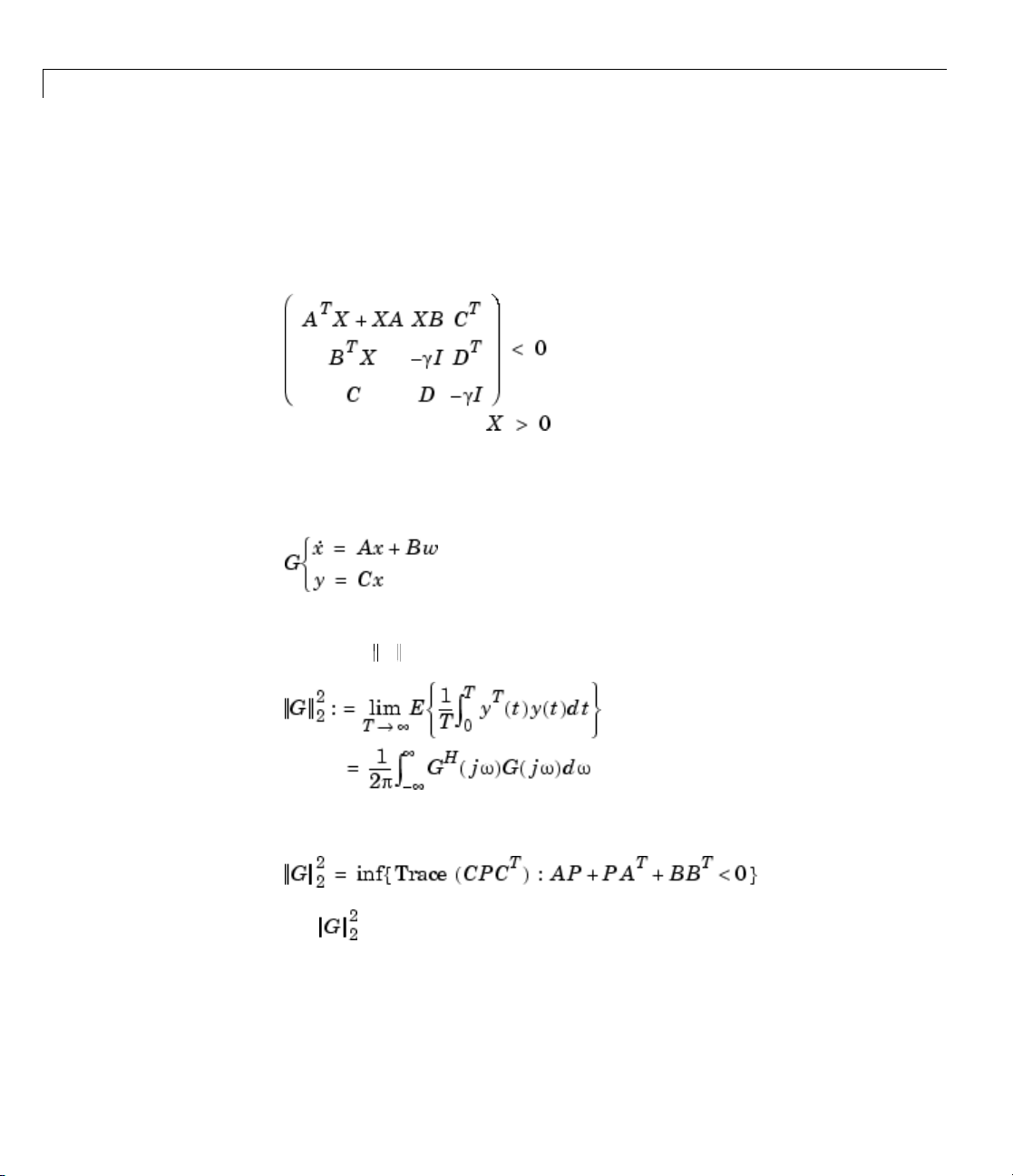
3 Introduction to Linear Matrix Inequalities

is the largest input/output gain over all bounded inputs u(t). This gain is the global minimum of the following linear objective minimization problem [1], [25], [26].

Minimize γ over X = X

and γ such that

LQG Performance

For a stable LTI system

where w is a white noise disturbance with unit covariance, the LQG or H performance G2is defined by

3-8

It can

be shown that

Hence is the global minimum of the LMI problem. Minimize Trace (Q) over the symmetric matrices P,Q such that

LMIs and LMI Problems

Again this is a linear objective minimization problem since the objective Tra ce (Q) is linear in the decision variables (free entries of P,Q).

3-9

3 Introduction to Linear Matrix Inequalities

Further Mathematical Background

Efficient interior-point algorithm s are now available to solve the three generic LMI problems Equation 3-2–Equation 3-4 defined in “Three Generic LM I Problems” on page 3-5. These algorithms have a polynomial-time complexity. That is, the number N(ε) of flops needed to compute an ε-accurate s olution is bounded by

log(V/ε)

where M is the total row size of the LMI system, N is the total number of scalar decision variables, and V is a data-dependent scaling factor. Robust Control Toolbox softw are implements the Projective Algorithm of Nesterov and Nemirovski [20], [19]. In addition t o its polynomial-time complexity, this algorithm does not require an initial feasible point for the linear objective minimization problem Equation 3-3or the generalized eigenvalue minimization problem Equation 3-4.

Some LMI problems are formulated in terms of inequalities rather than strict inequalities. For instance, a variant of Equation 3-3 is

3-10

Minimize c

x subject to A(x)<0.

While this distinc tion is immaterial in general, it matters when A(x)canbe made negative semi-definite but not negative definite. A simple example is

(3-6)

Such problems cannot be handled directly by interior-point methods which require strict feasibility of the LMI constraints. A well-posed reformulation of Equation 3-5 would be

Minimize c

x subject to x ≥ 0.

Keeping this subtlety in mind, we always use strict inequalities in this manual.

Bibliography

[1] Anderson, B.D.O., and S. Vongpanitlerd, Network Analysis, Prentice-Hall, Englewood Cliffs, 1973.

[2]Apkarian,P.,P.Gahinet,andG.Becker,“Self-ScheduledH

∞

Control of Linear Parameter-Varying Systems,” Proc. Amer. Contr. Conf., 1994, pp. 856-860.

[3] Bambang, R., E. Shimemura, and K. Uchida, “Mixed H

/H∞Control with

Pole Placement,” State-Feedback Case, Proc. Amer. Contr. Conf., 1993, pp. 2777-2779.

[4] B armish, B.R., “Stabilization of Uncertain Systems via Linear Control,” IEEE Trans. Aut. Contr., AC–28 (1983), pp. 848-850.

[5] Becker, G., and Packard, P., “Robust Performance of Linear-Parametrically Varying Systems Using Parametrically-Dependent Linear Feedback,” Systems and Control Letters, 23 (1994), pp. 205-215.

[6] Bendsoe, M.P., A. Ben-Tal, and J. Zowe, “Optimization M ethods for Truss Geometry and Topology Design,” to appear in Structural Optimization.

[7] Ben-Tal, A., and A. Nemirovski, “Potential Reduction Polynomial-Time Method for Truss Topology Design,” to a pp ea r in SIAM J. Contr. Opt.

[8] Boyd, S., and Q. Yang, “Structured and Simultaneous Lyapunov Functions for System Stability Problems,” Int. J. Contr., 49 (1989), pp. 2215-2240.

[9] Boyd, S., L. El Ghaoui, E. Feron, and V. Balakrishnan, Linear Matrix Inequalities in Systems and Control Theory, SIAM books, Philadelphia, 1994.

[10] C hilali, M., and P. Ga h inet, “H

∞

Design with Pole Placement Constraints: an LMI Approach,” to appear in IEEE Trans. Aut. Contr.AlsoinProc. Conf. Dec. Contr., 1994, pp. 553-558.

[11] Gahinet, P., and P. Apkarian, “A Linear Matrix Inequality Approach to

∞

Control,” Int. J. Robust and Nonlinear Contr., 4 (1994), pp. 421-448.

3-11

3 Introduction to Linear Matrix Inequalities

[12] Gahinet, P., P. Apkarian, and M. Chilali, “Affine Parameter-Dependent Lyapunov Functions for Real Parametric Uncertainty,“ Proc. Conf. Dec. Contr., 1994, pp. 2026-2031.

[13] Haddad, W.M., and D.S. Berstein, “Parameter-Dependent Lyapunov Functions, Constant Real Parameter Uncertainty, and the Popov Criterion in Robust Analysis and Synthesis: Part 1 and 2,” Proc. Conf. Dec. Contr., 1991, pp. 2274-2279 and 2632-2633.

[14] Iwasaki, T., and R.E. Skelton, “All Controllers for the General H

∞

Control Problem: LMI Existence Conditions and State-Space Formulas,” Automatica, 30 (1994), pp. 1307-1317.

[15] Horisberger, H.P., and P.R. Belanger, “Regulators for Linear Time-Varying Plants with Uncertain Parameters,” IEEE Trans. Aut. Contr., AC–21 (1976), pp. 705-708.

[16] How, J.P., and S.R. Hall, “Connection between the Popov Stability Criterion and Bounds for Real Parameter Uncertainty,” Proc. Amer. Contr. Conf., 1993, pp. 1084-1089.

[17] Khargonekar, P.P., and M.A. Rotea, “Mixed H

/H∞Control: a Convex

Optimization Approach,” IEEE Trans. Aut. Contr., 39 (1991), pp. 824-837.

[18] Masubuchi,I.,A.Ohara,andN.Suda,“LMI-BasedControllerSynthesis:

A Unified Formulation and Solution,” submitted to Int. J. Robust and Nonlinear Contr., 1994.

[19] Nemirovski, A., and P. Gahinet, “The Projective Meth od for Solving Linear Matrix Inequalities,” Proc. Amer. C ontr. Conf., 1994, pp. 840-844.

[20] Nesterov , Yu, and A. Nemirovski, Interior Point Polynomial Methods in Convex Programming: Theory and Applications, SIAM Books, Philadelphia,

1994.

3-12

[21] Packard, A., and J.C. Doyle, “The Complex Structured Singular Value,” Automatica, 29 (1994), pp. 71-109.

[22] Popov, V.M., “Absolute Stability of Nonlinear Systems o f Automatic Control,” Automation and Remote Control, 22 (1962), pp. 857-875.

Bibliography

[23] Scherer, C., “Mixed H2H∞Control,” to appear in Trends in Control: A European Perspective, volume of the special contributions to the ECC 1995.

[24] Stein, G., and J.C. Doyle, “Beyond Singular Values and Loop Shapes,” J. Guidance, 14 (1991), pp. 5-16.

[25] Vidyasagar, M., Nonlinear System Analysis, Prentice-Hall, Englewood Cliffs, 1992.

[26] Willems, J.C., “Least-Squares Stationary Optimal Control and the Algebraic Riccati Equation,” IEEE Trans. Aut. Contr., AC–16 (1971), pp. 621-634.

[27] Young, P.M., M.P. Newlin, and J.C. Doyle, “Let’s Get Real,” in Robust Control Theory, Springer Verlag, 1994, pp. 143-174.

[28] Zames, G., “On the Input-Output Stability of Time-Varying Nonlinear Feedback Systems, Part I and II,” IEEE Trans. Aut. Contr., AC–11 (1966), pp. 228-238 and 465-476.

3-13

3 Introduction to Linear Matrix Inequalities

3-14

Mathworks ROBUST CONTROL TOOLBOX 3 user guide

Specifications and Main Features

Frequently Asked Questions

User Manual