Mathworks ROBUST CONTROL TOOLBOX 3 Reference

Robust Control Too

Reference

Gary Balas
Richard Chiang
Andy Packard
Michael Safonov

lbox™ 3

How to Contact The MathWorks

www.mathworks.
comp.soft-sys.matlab Newsgroup
www.mathworks.com/contact_TS.html T echnical Support

[e-mail] Product enhancement suggestions
bugs@mathwo
[e-mail] Documentation error reports
[e-mail] Order status, license renewals, passcodes
info@mathwo

com

rks.com

rks.com

Web

Bug reports

Sales, prici

ng, and general information

508-647-7000 (Phone)

508-647-7001 (Fax)

The MathWorks, Inc.
3 Apple Hill Drive
Natick, MA 01760-2098

For contact information about worldwide offices, see the MathWorks Web site.

Robust Control Toolbox™ Reference

© COPYRIGHT 2005–2010 by The MathWorks, Inc.

The software described in this document is furnished under a license agreement. The software may be used
or copied only under the terms of the license agreement. No part of this manual may be photocopied or
reproduced in any form without prior written c onsent from The MathWorks, Inc.

FEDERAL ACQUISITION: This provision applies to all acquisitions of the Program and Documentation
by, for, or through the federal government of the United States. By accepting delivery of the Program
or Documentation, the gover nment hereby agrees that this software or documentation qualifies as
commercial computer software or commercial computer software documentation as such terms are used
or defined in FAR 12.212, DFARS Part 227.72, and DFARS 252.227-7014. Accordingly, the terms and
conditions of this Agreement and only those rights specified in this Agreement, shall pertain to an d gove rn
theuse,modification,reproduction,release,performance,display,anddisclosureoftheProgramand
Documentation by the federal government (or other entity acquiring for or through the federal government)
and shall supersede any conflicting contractual terms or conditions. If this License fails to meet the
government’s needs or is inconsistent in any respect with federal procurement law, the government agrees
to return the Program and Documentation, unused, to The MathWorks, Inc.

Trademarks

MATLAB and Simulink are registered trademarks of The MathWorks, Inc. See

www.mathworks.com/trademarks for a list of additional trademarks. Other product or brand

names may be trademarks or registered trademarks of their respective holders.

Patents

The MathWorks products are protected by one or more U.S. patents. Please see

www.mathworks.com/patents for more information.

Revision History

September 2005 First printing New for Version 3.0.2 (Release 14SP3)
March 2006 Online only Revised for Version 3.1 (Release 2006a)
September 2006 Online only Revised for Version 3.1.1 (Release 2006b)
March 2007 Online only Revised for Version 3.2 (Release 2007a)
September 2007 Online only Revised for Version 3.3 (Release 2007b)
March 2008 Online only Revised for Version 3.3.1 (Release 2008a)
October 2008 Online only Revised for Version 3.3.2 (Release 2008b)
March 2009 Online only Revised for Version 3.3.3 (Release 2009a)
September 2009 Online only Revised for Version 3.4 (Release 2009b)
March 2010 Online only Revised for Version 3.4.1 (Release 2010a)

Function Reference

1

Uncertain Elements ................................ 1-3

Contents

Uncertain Matrices and Systems

Manipulation of Uncertain Models

Interconnection of Uncertain Models

Model Order Reduction

Robustness and Worst-Case Analysis

Robustness Analysis for Parameter-Dependent Systems

(P-Systems)

Controller Synthesis

µ-Synthesis

Sampled-Data Systems

Gain Scheduling

..................................... 1-7

........................................ 1-9

................................... 1-10

............................ 1-5

............................... 1-8

............................. 1-10

.................... 1-3

.................. 1-4

................ 1-5

................ 1-6

Frequency-Response Data (FRD) Models

Supporting Utilities

LMIs

.............................................. 1-11

LMI Systems
LMI Characteristics

................................ 1-11

..................................... 1-11

............................... 1-12

............ 1-10

v

LMI Solvers ...................................... 1-12

Validation of Res ults
Modification of Systems of LMIs

............................... 1-13

..................... 1-13

2

3

Simulink

.......................................... 1-13

Functions — Alphabetical List

Block Reference

Index

vi Contents

Function Reference

Uncertain Elements (p. 1-3) Functions for building uncertain

elements

1

Uncertain Matrices and Systems
(p. 1-3)

Manipulation of Uncertain Models
(p. 1-4)

Interconnection of Uncertain Models
(p. 1-5)

Model O rder Reduction (p. 1-5) Functions for generating low-order

Robustness and Worst-Case Analysis
(p. 1-6)

Robustness Analysis for
Parameter-Dependent Systems
(P-Systems) (p. 1-7)

Controller Synthesis (p. 1-8) H

µ-Synthesis (p. 1-9) Structured singular value control

Sampled-Data Systems (p. 1-10) Functions for analyzin g

Gain Scheduling (p. 1-10) Functions for synthesizing

Functions for building uncertain
matrices and systems

Functions for transforming and
analyzing uncertain models

Functions for connecting uncertain
models

approximations to plant and
controller models

Functions for characterizing
system robustness and worst-case
performance

Functions for analyzing P-Systems

control design functions

∞

design functions

sampled-data systems

gain-scheduled controllers

1 Function Reference

Frequency-Response Data (FRD)
Models (p. 1-10)

Supporting Utilities (p. 1-11) Additional functions for working

LMIs (p. 1-11) Functions for building and

Simulink (p. 1-13) Functions for using with Simulink

Functions for operating on FRD
models

with systems containing uncertain
elements

solving systems of Linear Matrix
Inequalities

models

1-2

Uncertain Elements

Uncertain Elements

Uncertain

ucomplex

ucomplexm

udyn

ultidyn

ureal

Matrices and Systems

diag

randatom

randumat

randuss

ufrd

umat

uss

Create uncertain complex param eter

Create uncertain complex matrix

Create unstructured uncertain
dynamic system object

Create uncertain linear
time-invariant object

Create uncertain real parameter

Diagonalize vector of uncertain
matrices and systems

Generate random uncertain atom
objects

Generate random uncertain umat
objects

Generate stable, random uss objects

Create uncertain frequency response
data (

ufrd) object, or convert another

model type to

Create uncertain matrix

Specify uncertain state space models
or convert LTI model to uncertain
state space model

ufrd model

1-3

1 Function Reference

Manipulation of Uncertain Models

actual2normalized

gridureal

isuncertain

lftdata

normalized2actual

repmat

simplify

squeeze

usample

uss/ssbal

usubs

Calculate normalized distance
between uncertain atom nominal
value and specified value

Grid ureal parameters uniformly
over their range

Check whether argument is
uncertain class type

Decompose uncertain objects into
fixednormalizedandfixeduncertain
parts

Convert value for atom in normalized
coordinates to corresponding actual
value

Replicate and tile array

Simplify representation of uncertain
object

Remove singleton dimensions for

umat objects

Generate random samples of
uncertain variables

Scale state/uncertainty while
preserving uncertain input/output
map of uncertain system

Substitute given values for uncertain
elements of uncertain objects

1-4

Interconnection of Uncertain Models

Interconnection of Uncertain M odels

iconnect

icsignal

imp2exp

stack

sysic

Model Order Reduction

balancmr

bstmr

hankelmr

hankelsv

imp2ss

modreal

ncfmr

Create empty iconnect
(interconnection) objects

Create icsignal object of specified
dimension

Convertimplicitlinear relationship
to explicit input-output relation

Construct array by stacking
uncertain matrices, models, or
arrays

Build interconnections of certain and
uncertain matrices and systems

Balanced model truncation via
square root method

Balanced stochastic model
truncation (BST) via Schur method

Hankel minimum degree
approximation (M DA) without
balancing

Compute Hankel singular
values for stable/unstable or
continuous/discrete system

System realization via Hankel
singular value decomposition

Modal form realization and
projection

Balanced model truncation for
normalized coprime factors

1-5

1 Function Reference

reduce

Simplified access to Hankel singular
value based model reduction
functions

schurmr

Balanced model trunca t ion via Schur
method

slowfast

Slow and fast modes decomposition

Robustness and Worst-Case Analysis

cpmargin

gapmetric

loopmargin

loopsens

mussv

mussvextract

ncfmargin

popov

robopt

robustperf

Coprime stability margin of
plant-controller feedback loop

Compute upper bounds on
Vinnicombe
between two systems

Stability margin analysis of L TI a nd
Simulink

Sensitivity functions of
plant-controller feedback loop

Compute bounds on structured
singular value (µ)

Extract muinfo structure returned
by

Calculate normalized coprime
stability margin of plant-controller
feedback loop

Perform Popov robust stability test

Create options object for use with

robuststab and robustperf

Robust performance margin of
uncertain m ultivariable system

mussv

gap and nugap distances

®

feedback loops

1-6

Robustness Analysis for Parameter-Dependent Systems (P-Systems)

robuststab

Calculate robust stability margins of
uncertain m ultivariable system

wcgain

Calculate bounds on worst-case gain
of uncertain system

wcgopt

wcmargin

Create options object for use with

wcgain, wcsens,andwcmargin

Worst-case disk stability margins of
uncertain feedback loops

wcnorm

wcsens

Worst-case norm of uncertain matrix

Calculateworst-casesensitivityand
complementary sensitivity functions
of plant-co ntro ller feedback loop

Robustness Analysis for Parameter-Dependent Systems
(P-Systems)

aff2pol

decay

ispsys

pdlstab

pdsimul

polydec

Convert affine parameter-dependent
models to polytopic models

Quadratic decay rate of polytopic or
affine P-systems

True for parameter-dependent
systems

Assess robust stability of polytopic
or parameter-dependent system

Time response of
parameter-dependent system
along given parameter trajectory

Compute polytopic coordinates with
respect to box corners

1-7

1 Function Reference

psinfo

pvec

pvinfo

quadperf

quadstab

Controller Synthesis

augw

h2hinfsyn

h2syn

hinfsyn

loopsyn

ltrsyn

mixsyn

Inquire about polytopic or
parameter-dependent systems
created with

psys

Specify range and rate of variation
of uncertain or time-varying
parameters

Describe parameter vector specified
with

pvec

Compute quadratic H performance
of polytopic or parameter-dependent
system

Quadratic stability of polytopic or
affine pa ra m eter-de pe n de nt systems

State-space or transfer function
plant augmentation for use in
weighted mixed-sensitivity H and H
loopshaping design

Mixed H/H synthesis with p ole
placement constraints

H control synthesis for LTI plant

Compute H optimal controller for
LTI plant

H optimal controller synthesis for
LTI plant

LQG loop transfer-function recovery
(LTR) control synthesis

H mixed-sensitivity synthesis
method for robust control
loopshaping design

1-8

µ-Synthesis

µ-Synthesis

mkfilter

ncfsyn

cmsclsyn

dkitopt

dksyn

drawmag

fitfrd

fitmagfrd

genphase

Generate Bessel, Butterworth,
Chebyshev, or RC filter

Loop shaping design using
Glover-McFarlane method

Approximately solve
constant-matrix, upper bound
µ-synthesis problem

Create options object for use with

dksyn

Robust controller design using
µ-synthesis

Mouse-based tool for sketching and
fitting

Fit frequency response data with
state-space model

Fit frequency response magnitude
data with minimum-phase
state-space model using
log-Chebychev magnitude design

Fit single-in put/single-output
magnitude data with real, rational,
minimum-phase transfer function

1-9

1 Function Reference

Sampled-Data Systems

Gain Sched

sdhinfnorm

sdhinfsyn

sdlsim

uling

hinfgs

Compute L norm of continuous-time
system in feedback with
discrete-time system

Compute H controller for
sampled-data system

Time response of sampled-data
feedback system

Synthesis of gain-scheduled H
controllers

Frequency-Response Data (FRD) Models

frd/log

frd/rc

frd/s

frd/

frd/

log

ond

chur

semilogx

svd

Log-log

LAPACK
estima

Schur

Semil

ular value decomposition of

Sing

ct

obje

scale plot of

reciprocal condition

tor of

frd object

decomposition of

og scale plot of

frd objects

frd object

frd object

frd

1-10

Supporting Utilities

Supporting Utilities

LMIs

bilin

dmplot

mktito

sectf

skewdec

symdec

LMI Sys

LMI Ch

LMI So

Vali

Mod
(p.

tems (p. 1-11)

aracteristics (p. 1-12)

lvers (p. 1-12)

dation of Results (p. 1-13)

ification of Systems of LMIs

1-13)

Multivariable bilinear transform of
frequency (s or z)

Interpret disk gain and phase
margins

Partition LT
two-input/t

State-spac
transforma

Form skew-symmetric matrix

Form symmetric matrix

Isysteminto

wo-output system

e sector bilinear

tion

LMI Systems

tlmis

ge

miedit

l

lmiterm

lmivar

ternal description of LMI system

In

pecify or display systems of LMIs

S

s MATLAB

a

pecify term content of LMIs

S

Specify matrix variables in LMI
problem

®

expressions

1-11

1 Function Reference

newlmi

setlmis

LMI Characteristics

dec2mat

decinfo

decnbr

lmiinfo

lminbr

mat2dec

matnbr

Attach identifying tag to LMIs

Initialize description of LMI system

Givenvaluesofdecisionvariables,
derive corresponding values of
matrix variables

Describe how entries of matrix
variable X relate to decision
variables

Total number of decision variables
in system of LMIs

Information about variables and
term content of LMIs

Return number of LMIs in LMI
system

Extract vector of decision variables
from matrix variable values

Number of matrix variables in
system of LMIs

1-12

LMI Solvers

defcx

feasp

gevp

mincx

Help specify cTx objectives for mincx
solver

Compute solution to given system of
LMIs

Generalized eigenvalue
minimization under LMI constraints

Minimize linear objective under LMI
constraints

Validation of Results

Simulink

®

evallmi

Given particular instance of decision
variables, evaluate all variable
terms in system of LMIs

showlmi

Return left- and right-hand sides of
LMI after evaluation of all variable
terms

Modification of Systems of LMIs

bilin

dmplot

mktito

sectf

skewdec

symdec

Multivariable bilinear transform of
frequency (s or z)

Interpret disk gain and phase
margins

Partition LTI system into
two-input/two-output system

State-space sector bilinear
transformation

Form skew-symmetric matrix

Form symmetric matrix

Simulink

ufind

ulinearize

Find uncertain variables in Simulink
model

Linearize Simulink model with
Uncertain State Space block

1-13

1 Function Reference

1-14

Functions — Alphabetical List

2

actual2normalized

Purpose Calculate normalized distance between uncertain atom nominal value

and specified value

Syntax NDIST = actual2normalized(A,V)

Description NDIST = actual2normalized(A,V) is the normalized distance b etw een

thenominalvalueoftheuncertainatom
is a ureal,thenNDIST may be positive or negative, reflecting that V is
greater than, or less than the nominal value. If
uncertain atom, then

fVis an array of values, then NDIST is an array of normalized

I
distances.

ndist is nonnegative.

A and the given value V.IfA

A is any other class of

The robustness margins computed in
serve as bounds for the normalized distances in NDIST. For example, if
an uncertain system has a stability margin of 1.4, this system is stable
when the normalized distance of the uncertain element values from the
nominal is less than 1.4.

robuststab and robustperf

Examples Uncertain Real Parameter with Symmetric Range

For uncertain real parameters whose range is symmetric about their
nominal value, the normalized distance is intuitive, scaling linearly
with the numerical difference from the uncertain real parameter’s
nominal value.

Create
the nom
Point
while
the no

uncertain real parameters with a range that is symmetric about

inal value, where each end point is 1 unit from the nominal.

sthatlieinsidetherangearelessthan1unitfromthenominal,

points that lie outside the range are g reater than 1 unit from

minal.

a = ureal('a',3,'range',[1 5]);
actual2normalized(a,[1 3 5])
ans =

-1.0000 -0.0000 1.0000
actual2normalized(a,[2 4])
ans =

2-2

actual2normalized

-0.5000 0.5000
actual2normalized(a,[0 6])
ans =

-1.5000 1.5000

Graph the normalized distance for several values. The nominal point is
shown as a red circle. Note that the relationship between a normalized
distance and a numerical difference is linear.

values = linspace(-3,9,250);
ndist = actual2normalized(a,values);
plot(values,ndist)

Uncertain Real Parameter with Nonsymmetric Range

Next, create an unasymmetric parameter. It still is true that the
end points are 1 normalized unit from nominal, and the nominal is
0 normalized units from nominal, moreover points inside the range
are less than 1 unit from nominal, and points outside the range are
greater than 1 unit from nominal. However, the relationship between
the normalized distance and numerical difference is nonlinear.

2-3

actual2normalized

au = ureal('a',4,'range',[1 5]);
actual2normalized(a,[1 4 5])
ans =

actual2normalized(a,[2 4.5])
ans =

actual2normalized(a,[0 6])
ans =

Graph the normalized distance for several values. Note that the
relationship between normalized distance and numerical difference is
very nonlinear.

ndistu = actual2normalized(au,values);
plot(values,ndistu,au.NominalValue,0,'ro')

-1.0000 0.5000 1.0000

-0.5000 0.7500

-1.5000 1.5000

2-4

actual2normalized

Algorithm For details on the normalize distance, s ee “Normalizing Functions for

Uncertain Atoms” in the Robust Control Toolbox™ User’s Guide.

See Also normalized2actual

robuststab

robustperf

2-5

aff2pol

Purpose Convert affine parameter-dependent models to polytopic models

Syntax polsys = aff2pol(affsys)

Description aff2pol derives a polytopic representation polsys of the affine

parameter- dependent system

(2-1)

(2-2)

See Al

so

where p =(p
parameters taking values in a box or a polytope. The description
of this system should be specified with psys.

The vertex systems of
Equation 2-2 at the vertices p
matrices

for all corners pexof the parameter box or all vertices pexof the polytope
of parameter values.

psys

pvec

uss

,...,pn) is a vector of uncertain or time-varying real

1

polsys are the instances of Equation 2-1 and

of the parameter range, i.e., the SYSTEM

ex

affsys

2-6

augw

Purpose State-space or transfer function plant augmentation for use in weighted

mixed-sensitivity H

Syntax P = AUGW(G,W1,W2,W3)

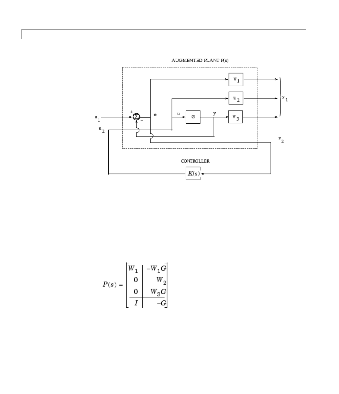
Description P = AUGW(G,W1,W2,W3) computes a state-space model of an augmented

LTI plant P(s) with weighting functions W
penalizing the error signal, control signal and output signal respectively
(see block diagram) so that the closed-loop transfer function matrix
is the weighted mixed sensitivity

where S, R and T are given by

and H2loopshaping design

∞

1

(s), W2(s), and W3(s)

The LTI systems S and T are called the sensitivity and complementary
sensitivity, respectively.

2-7

augw

Plant Augmentation

2-8

Algori

thm

For dimensional compatibility, each of the three weights W1, W2and
W

must be e ither empty, a scalar (SISO) or have respective input

3

dimensions N
is not needed, you may simply assign an empty matrix [ ]; e.g.,

AUGW(G,W1,[],W3)

below, but without the second row (without the row containing

The aug

Partitioning is embedded via P=mktito(P,NY,NU), which sets the
InputGroup and OutputGroup properties of P as follows

mented plant P(s) produced by is

, NU,andNYwhere G is NY-by-NU. If one of the weights

Y

is P(s) as in the “Algorithm” on page 2-8 section

P=

W2).

[r,c]=size(P);
P.InputGroup = struct('U1',1:c-NU,'U2',c-NU+1:c);
P.OutputGroup = struct('Y1',1:r-NY,'Y2',r-NY+1:r);

Examples s=zpk('s'); G=(s-1)/(s+1);

W1=0.1*(s+100)/(100*s+1); W2=0.1; W3=[];

P=augw(G,W1,W2,W3);

[K,CL,GAM]=hinfsyn(P); [K2,CL2,GAM2]=h2syn(P);

L=G*K; S=inv(1+L); T=1-S; sigma(S,'k',GAM/W1,'k-.',T,'r',GAM*G/W2,'r-.')

legend('S = 1/(1+L)','GAM/W1', 'T=L/(1+L)','GAM*G/W2',2)

augw

Limitations The transfer functions G, W

as

or, in the discrete-time case, as . Additionally, W1,

, W2and W3must be proper, i.e., bounded

1

2-9

augw

See Also h2syn

W2and W3should be stable. The plant G should be stabilizable and

detectable; else,

hinfsyn

mixsyn

mktito

P will not be stabilizable by any K.

2-10

balancmr

Purpose Balanced model truncation via square root method

Syntax GRED = balancmr(G)

GRED = balancmr(G,order)
[GRED,redinfo] = balancmr(G,key1,value1,...)
[GRED,redinfo] = balancmr(G,order,key1,value1,...)

Description balancmr returns a reduced order model GRED of G and a struct array

redinfo containing the error bound of the reduced model and Hankel

singular values of the original system.

The error bound is computed based on Hankel singular values of
a stable system these values indicate the respective state energy of the
system. Hence, reduced order can be directly determined by examining
the system Hankel singular values, σι.

With only one input argument
singular value plot of the original model and prompt for model order
number to reduce.

This method guarantees an error bound on the infinity norm of the

additive error

[1]:

This table describes input arguments for balancmr.

Argument Description

G

ORDER

G-GRED ∞ for well-conditioned model reduced problems

LTI model to be reduced. Without any other
inputs,
values of

(Optional) Integer for the desired order of the
reduced model, o r optionally a vector packed with
desired orders for batch runs

G, the function will show a Hankel

balancmr will plot the Hankel singular

G and prompt for reduced order

G.For

2-11

balancmr

A batch run of a serial of different reduced order models can be
generated by specifying

order = x:y, or a vector of positive integers.

By default, all the anti-stable part of a system is kept, because from
control stability point of view, getting rid of unstable state(s) is
dangerous to model a system.

’MaxError’ can be specified in the same fashion as an alternative for

'Order'. In this case, reduced order will be determined when the sum

of the tails of the Hankel singular values reaches the

’MaxError’.

This table lists the input arguments

'key' and its 'value'.

Argument Value Description

’MaxError’

Real number or
vector of different
errors

Reduce to achieve H

∞

error. When present,

'MaxError'overides ORDER

input.

’Weights’

{Wout,Win}

array

cell

Optimal1-by-2cellarrayof
LTI weights
and

Win (input). Defaults are

Wout (output)

both identity. Weights must
be invertible.

’Display’ 'on' or 'off'

’Order’

Integer, vector or
cell array

Display Hankel singular
plots (default

'off').

Order of reduced model. Use
only if not s pecified as 2nd
argument.

Weights on the original model input and/or output can make the model
reduction algorithm focus on some frequency range of interests. But
weights have to be stable, minimum phase and invertible.

This table describes output arguments.

2-12

balancmr

Argument Description

GRED

REDINFO

G can be stable or unstable, continuous or discrete.

Algorithm Given a state space (A,B,C,D) of a system and k, the desired reduced

order, the following steps will produce a similarity transformation to
truncate the original state space system to the k

LTI reduced order model. Becomes multidimensional
array when input is a serial of different model order
array

A STRUCT array with three fields:

•

REDINFO.ErrorBound (bound on G-GRED ∞)

• REDINFO.StabSV (Hankel SV of stable part of

G)

• REDINFO.UnstabSV (Hankel SV of unstable part

of G)

th

order reduced model.

1 Find the SVD of the controllability and observability grammians

P=U

pΣpVp

Q=UqΣqV

2 Find the square root of the grammians (left/right eigenvectors)

L

=UpΣ

p

Lo=UqΣ

3 Find the SVD of (L

T

L

Lp=UΣ V

o

T

T

q

1/2

p

1/2

q

T

Lp)

o

T

2-13

balancmr

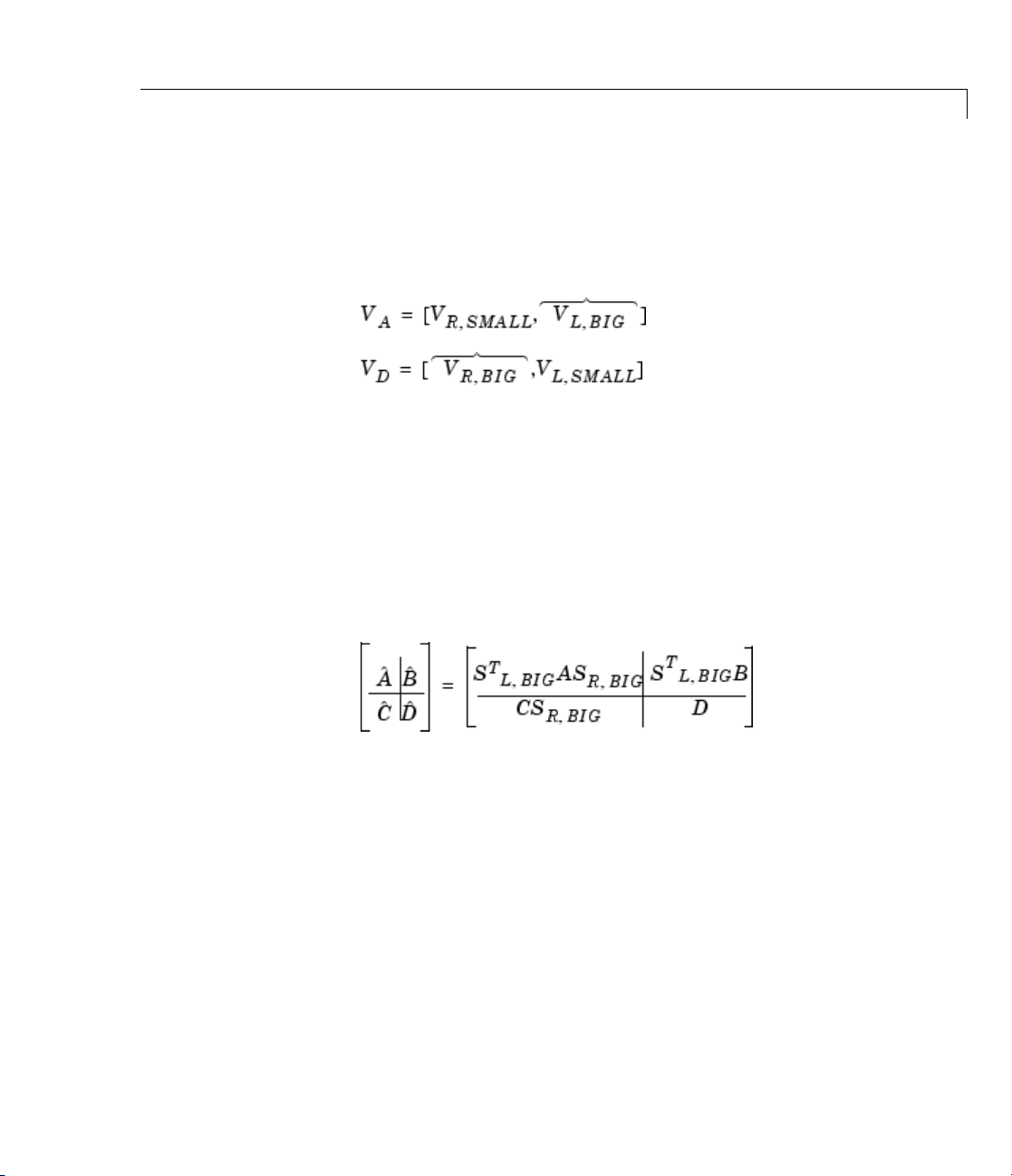
4 Then the left and right transformation for the final k

th

order reduced

model is

S

L,BIG=Lo

S

R,BIG=Lp

5 Finally,

The proof o

U(:,1:k) Σ(1;k,1:k))

V(:,1:k) Σ(1;k,1:k))

f the square root balance truncation algorithm can be found

-1/2

-1/2

in [2].

Examples Given a continuous or discrete, stable or unstable system, G,the

following commands can get a set of reduced order models based on
your selections:

rand('s
[g1, red

[g2, re
[g3, re
[g4, r
rand(
wt1 = r
wt2 = r
[g5,
for i

end

tate',1234); randn('state',5678);G = rss(30,5,4);

info1] = balancmr(G); % display Hankel SV plot

% and pr
dinfo2] = balancmr(G,20);
dinfo3] = balancmr(G,[10:2:18]);

edinfo4] = balancmr(G,'

'state',12345); randn('state',6789);

ss(6,5,5); wt1.d = eye(5)*2;
ss(6,4,4); wt2.d = 2*eye(4);

redinfo5] = balancmr(G, [10:2:18], '

=1:5

re(i); eval(['sigma(G,g' num2str(i) ');']);

figu

MaxError',[0.01, 0.05]);

ompt for order (try 15:20)

weight',{wt1,wt2});

2-14

balancmr

References [1] Glover, K., “All Optimal Hankel Norm Approximation o f Linear

Multivariable Systems, and Their Lµ-error Bounds,“ Int. J. Control,
Vol. 39, No. 6, 1984, p. 1145-1193

[2] Safonov, M.G., and R.Y. Chiang, “A Sc h ur Method for Balanced
Model Reduction,” IEEE Trans. on Automat. Contr., Vol. 34, No. 7,
July 1989, p. 729-733

See Also reduce

schurmr

hankelmr

bstmr

ncfmr

hankelsv

2-15

bilin

Purpose Multivariable bilinear transform of frequency (s or z)

Syntax GT = bilin(G,VERS,METHOD,AUG)

Description bilin computes the effect on a system of the frequency-variable

substitution,

The variable VERS denotes the transformation direction:

VERS= 1, forward transform or .

VERS=-1, reverse transform or .

This transformation maps lines and circles to circles and lines in the
complex plane. People often use this transformation to do sampled-data
control system design [1] or, in general, to do shifting of jω modes [2],
[3], [4].

2-16

Bilin computes several state-space bilinear transformations such as

backward rectangular, etc., based on the

Bilinear Transform Types

Method Type of bilinear transform

'BwdRec'

'FwdRec'

ard rectangular:

backw

AUG = T, the sampling period.

forward rectangular:

G=

AU

T, the sampling period.

METHOD you select

Bilinear Transform Types (Continued)

Method Type of bilinear transform

'S_Tust'

'S_ftjw'

shifted Tustin:

AUG = [Th], is the “shift” coefficient.

shifted jω-axis, bilinear pole-shifting,
continuous-time to continuous-time:

bilin

Exam

ples

AUG = [p

'G_Bilin'

Exam
tran

Con

Following is an example of four common “continuous to discrete” bilin
transformations for the sampled plant:

ple 1. Tustin continuous s-plane to discrete z-plane

sforms

sider the following continuous-time plant (sampled at 20 Hz):

METHOD = 'G_Bilin'

continuous-time to continuos-time:

AUG = .

2p1

].

, general bilinear,

2-17

bilin

A= [-1 1; 0 -2]; B=[1 0; 1 1];
C= [1 0; 0 1]; D=[0 0; 0 0];
sys = ss(A,B,C,D); % ANALOG
Ts=0.05; % sampling time
[syst] = c2d(sys,Ts,'
[sysp] = c2d(sys,Ts,'prewarp',40); % Pre-warped Tustin
[sysb] = bilin(sys,1,'
[sysf] = bilin(sys,1,'
w = logspace(-2,3,50); % frequencies to plot
sigma(sys,syst,sysp,sysb,sysf,w);

tustin'); % Tustin

BwdRec',Ts); % Backward Rectangular
FwdRec',Ts); % Forward Rectangular

2-18

Comparison of Four Bilinear Transforms from Example 1

Example 2. Bilinear continuous to continuous pole-shifting
’S_ftjw’

Design an H mixed-sensitivity controller for the ACC Benchmark plant

bilin

such that all closed-loop poles lie inside a circle in the left half of the
s-plane who se diameter lies on between points [p1,p2]=[-12,-2]:

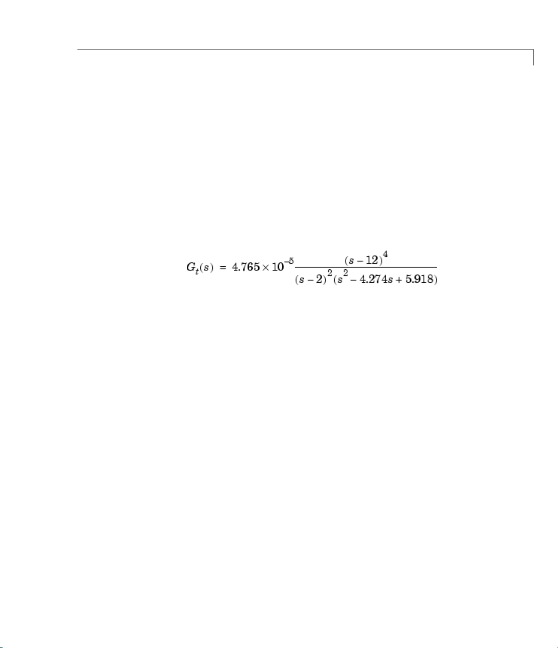
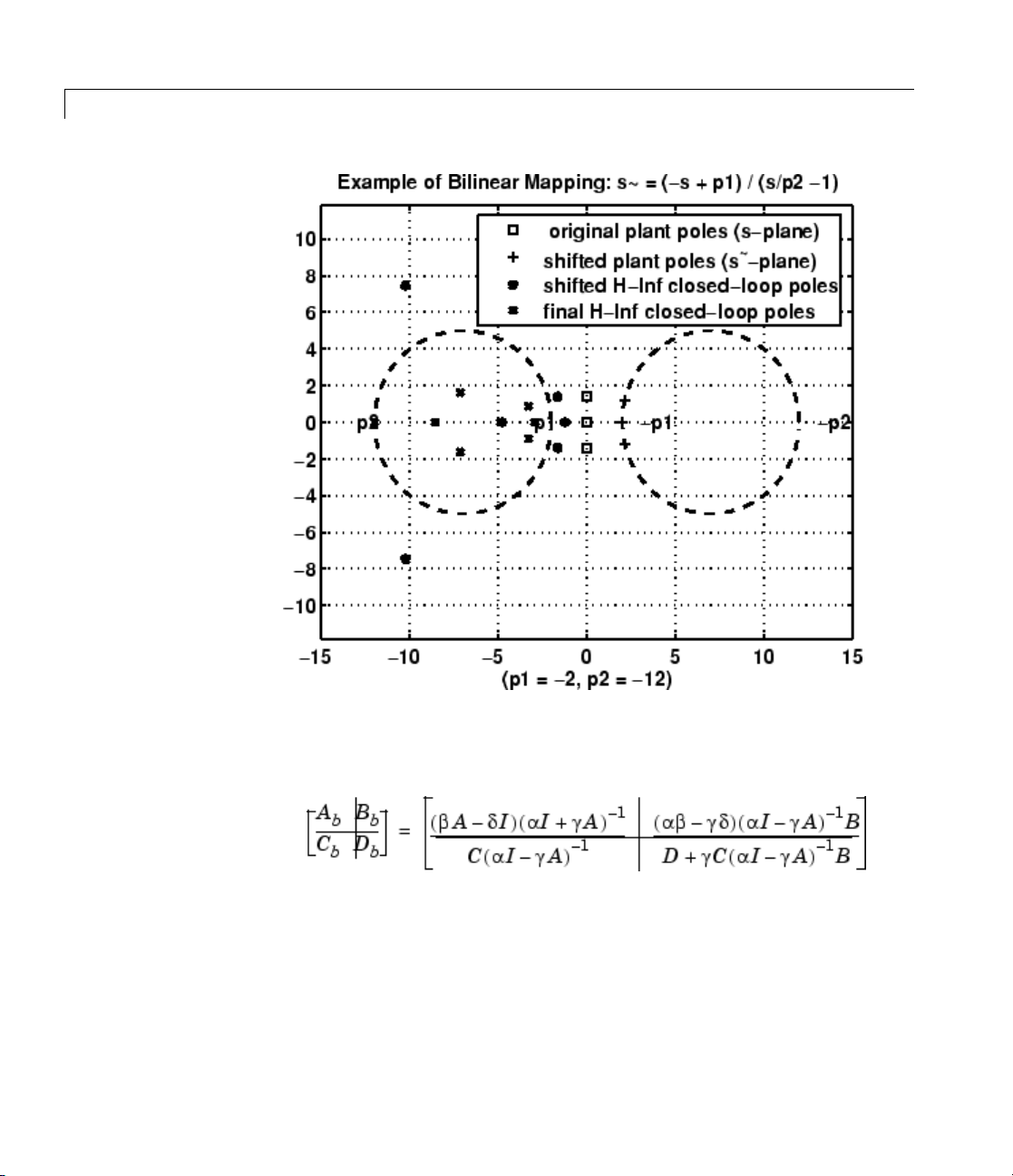
p1=-12; p2=-2; s=zpk('s');
G=ss(1/(s^2*(s^2+2))); % original unshifted plant
Gt=bilin(G,1,'Sft_jw',[p1 p2]); % bilinear pole shifted plant Gt
Kt=mixsyn(Gt,1,[],1); % bilinear pole shifted controller
K =bilin(Kt,-1,'

As shown in the following figure, closed-loop poles are placed in the left
circle

[p1 p2]. The shifted plant, which has its non-stable poles shifted

to the inside the right circle, is

Sft_jw',[p1 p2]); % final controller K

2-19

bilin

S_ftjw final closed-loop poles are inside the left [p1,p2] circle

Algorithm bilin employs the state-space formulae in [3]:

References [1] Franklin, G.F., and J.D. Powell, Digital Control of Dynamics System,

Addison-Wesley, 1980.

2-20

[2] Safonov, M.G., R.Y. Chiang, and H. Flashner, “H∞Control Synthesis
for a Large S pace Structure,” AIAA J. Guidance, Control and Dynamics,
14, 3, p. 513-520, May/June 1991.

bilin

[3] Safonov, M.G., “Imaginary-Axis Zeros in Multivariable H
Control”, in R.F. Curtain (editor), Modelling, Robustness and Sensitivity
Reduction in Control Systems,p. 71-81,Springer-Varlet,Berlin,1987.

[4] Chiang, R.Y., and M.G. Safonov, “H
Shifting Transform,” AIAA, J. Guidance, Control and Dynamics,vol.
15, no. 5, p. 1111-1117, September-October 1992.

See Also c2d

d2c

sectf

Optimal

∞

Synthesis using a Bilinear Pole

∞

2-21

bstmr

Purpose Balanced stochastic model truncation (BST) via Schur method

Syntax GRED = bstmr(G)

GRED = bstmr(G,order)
[GRED,redinfo] = bstmr(G,key1,value1,...)
[GRED,redinfo] = bstmr(G,order,key1,value1,...)

Description bstmr returns a reducedordermodelGRED of G and a struct array

redinfo containing the error bound of the reduced model and Hankel

singular values of the phase matrix of the original system [2].

The error bound is computed based on Hankel singular values of
the phase matrix of
respective state energy of the system. Hence, reduce d order can be
directly determined by examining these values.

G. For a stable system these values indicate the

With only one input argument
singular value plot of the phase matrix of
number to reduce.

This method guarantees an error bound on the infinity norm of the

multiplicative

for well-conditioned model reduction problems [1]:

This table describes input arguments for bstmr.

Argument Description

G

ORDER

GRED-1(G-GRED) ∞ or relative error G

LTI model to be reduced (without any other inputs
will plot its Hankel singular values and prompt
for reduced order)

(Optional) an integer for the desired order of the
reduced model, or a vector of desired orders for
batch runs

G, the function will show a Hankel

G and prompt for model order

-

-1(G-GRED) ∞

2-22

bstmr

A batch run of a serial of different reduced order models can be
generated by specifying
default, all the anti-stable part of a system is kept, because from control
stability point of v iew, getting rid of unstable state(s) is dangerous to
model a system.

’MaxError’ canbespecifiedinthesamefashionasanalternative

for

'ORDER'. In this case, reduced order will be determined w hen the

accumulated product of Hankel singular values shown in the above
equation reaches the

Argument Value Description

’MaxError’

’Display’ 'on' or 'off'

’Order’

order = x:y, or a vector of integers. By

’MaxError’.

Real num ber
or vector of
different errors

Reduce to achieve H∞error.

When present,

'MaxError'overides ORDER

input.

Display Hankel singular plots

Integer, vector or
cell array

(default

Order of reduced model. Use
only if not specified as 2nd

'off').

argument.

This table describes output arguments.

Argument Description

GRED

LTI reduced order model. Become multi-dimension
array when input is a serial of different model
order array.

REDINFO

A STRUCT array with three fields:

•

REDINFO.ErrorBound (bound on G

∞)

• REDINFO.StabSV (Hankel SV of stable part

of G)

-1

(G-GRED)

2-23

bstmr

Argument Description

• REDINFO.UnstabSV (Hankel SV of unstable

part of G)

G can be stable or unstable, continuous or discrete.

Algorithm Given a state space (A,B,C,D) of a system and k, the desired reduced

order, the following steps will produce a similarity transformation to
truncate the original state space system to the k

1 Find the controllability grammian P and observability grammian Q

of the left spectral factor Φ = Γ(σ)Γ*(-σ)=Ω*(-σ)Ω(σ)bysolvingthe
following Lyapunov and Riccati equations

th

order reduced model.

AP + PA

B

W

T

+BBT=0

=PCT+BD

T

QA + ATQ+(QBW-CT)(-DDT)(QBW-CT)T=0

2 Find the Schur decomposition for PQ in both ascending and

descending order, respectively,

2-24

bstmr

3 Find the left/right orthonormal eigen-bases of PQ associated with

the k

*

(W

(s))-1G(s).

th

big Hankel singular values of the all-pass phase matrix

k

4 Find the SVD of (V

5 Form the left/right transformation for the final k

T

V

L,BIG

)=U ΣςΤ

R,BIG

th

order reduced

model

S

L,BIG=VL,BIG

S

R,BIG=VR,BIG

6 Finally,

U Σ(1:k,1:k)

V Σ(1:k,1:k)

-1/2

-1/2

The pr

oof of the Schur BST algorithm can be found in [1].

2-25

bstmr

Note The BST model reduction theory requires that the original model

D matrix be full rank, for otherwise the Riccati solver fails. For any
problem with strictly proper model, you can shift the jω-axis via
such that BST/REM approximation can be achieved up to a particular
frequency range of interests. Alternatively, you can attach a small but
full rank D matrix to the original problem but remove the D matrix of
the reduced order model afterwards. As long as the size of D matrix is
insignificant inside the control bandwidth, the reduced order model
should be fairly close t o the true model. By defau lt, the
will assign a full rank D matrix scaled by 0.001 of the minimum
eigenvalue of the original model, if its D matrix is not full rank to begin
with. This serves the purpose for most problems if user does not want to
go through the trouble of model pretransformation.

Examples Given a continuous or discrete, stable or unstable system, G,the

following commands can get a set of reduced order models based on
your selections:

bilin

bstmr program

rand('state',1234); randn('state',5678);
G = rss(30,5,4); G.d = zeros(5,4);
[g1, redinfo1] = bstmr(G); % display Hankel SV plot

% and prompt for order (try 15:20)
[g2, redinfo2] = bstmr(G,20);
[g3, redinfo3] = bstmr(G,[10:2:18]);
[g4, redinfo4] = bstmr(G,'
for i = 1:4

figure(i); eval(['sigma(G,g' num2str(i) ');']);

end

MaxError',[0.01, 0.05]);

References [1] Zhou, K., “Frequency-weighted model reduction with L∞ error

bounds,” Syst.Contr.Lett., Vol. 21, 115-125, 1993.

[2] Safonov, M.G., and R.Y. Chiang, “Model Reduction for Robust
Control: A Schur Relative Error Method,” InternationalJ.ofAdaptive
Control and Signal Processing, Vol. 2, p. 259-272, 1988.

2-26

See Also reduce

balancmr

hankelmr

schurmr

ncfmr

hankelsv

bstmr

2-27

complexify

Purpose Replace ureal atoms by summations of ureal and ucomplex (or

ultidyn)atoms

Syntax MC = complexify(M,alpha)

MC = complexify(M,alpha,'ultidyn')

Description The command complexify replaces ureal atomswithsumsofureal

and ucomplex atoms using usubs. Optionally, the sum can consist of a

ureal and ultidyn atom.

complexify is used to improve the conditioning of robust stability

calculations (

ureal uncertain elements.

MC = complexify(M,alpha) results in each ureal atom in MC having

the same
M. If

Range is the range of one ureal atom from M, then the range of the

corresponding ureal atom in

Range(1)+alpha*diff(Range)/2 Range(2)-alpha*diff(Range)/2]

[

robuststab) for situations when there are predominantly

Name and NominalValue as the corresponding ureal atom in

MC is

The net effect is that the same real range is covered with a real and
complex uncertainty. The real parameter range is reduced by equal
amounts at each end, and
reduction in the total range. The
in range back into

ucomplex atom has NominalValue of 0, and Radius equal to

The

alpha*diff(Range). Its name is the name of the original ureal atom,

MC, but as a ball with real and imaginary parts.

appended with the characters

MC = complexify(M,alpha,'ultidyn') is the same, except that

gain-bounded

ultidyn atom has its Bound equal to alpha*diff(Range).

ultidyn atoms are used instead of ucomplex atoms. The

alpha represents (in a relative sense) the

ucomplex atom will add this reduction

'_cmpxfy'.

Examples See Robust Control Toolbox d emo “Getting Reliable Estimates of

Robustness Margins” for an example of how complexify is used in
robustness analysis.

2-28

complexify

For illustrative purposes only, create a uncertain real parameter, cast it
to a uncertain matrix, and apply a 10% complexification. Finally, make
a scatter plot of the values that the complexified matrix (scalar) can
take a s well as the values of the original uncertain real p aram e ter.

a = umat(ureal('a',2.25,'Range',[1.5 3]));
b = complexify(a,.1);
as = usample(a,200);
bs = usample(b,4000);
plot(real(bs(:)),imag(bs(:)),'.',real(as(:)),imag(as(:)),'r.')

See Also icomplexify

robuststab

2-29

cmsclsyn

Purpose Approximately solve constant-matrix, upper bound µ-synthesis problem

Syntax [QOPT,BND] = cmsclsyn(R,U,V,BlockStructure);

[QOPT,BND] = cmsclsyn(R,U,V,BlockStructure,opt);
[QOPT,BND] = cmsclsyn(R,U,V,BlockStructure,opt,qinit);
[QOPT,BND] = cmsclsyn(R,U,V,BlockStructure,opt,'random',N)

Description cmsclsyn approximately solves the constant-matrix, upper bound

µ-synthesis problem by minimization,

for given matrices R Cnxm, U Cnxr, V Ctxm,andasetΔ ⊂ Cmxn.This
applies to constant matrix data in R, U, and V.

[QOPT,BND] = cmsclsyn(R,U,V,BlockStructure) minimizes, by

choice of Q.

mussv(R+U*Q*V,BLK), BND.ThematricesR,U and V are constant

matrices of the appropriate dimension.
specifying the perturbation blockstructure as defined for

QOPT is the optimum value of Q, the upper bound of

BlockStructure is a matrix

mussv.

2-30

[QOPT,BND] = cmsclsyn(R,U,V,BlockStructure,OPT) uses the

options specified by
information. The default value for

[QOPT,BND] = cmsclsyn(R,U,V,BlockStructure,OPT,QINIT)

OPT in the c alls to mussv.Seemussv for more

OPT is 'cUsw'.

initializes the iterative computation from Q = QINIT.Becauseofthe
nonconvexity of the overall problem, diffe rent starting points often yield
different final answers. If
computation is performed multiple times - the
initialized at Q =

QINIT(:,:,i). The output arguments are associated

QINIT is an N-D array, then the iterative

i’th optimization is

with the best solution obtained in this brute force approach.

[QOPT,BND] = cmsclsyn(R,U,V,BlockStructure,OPT,'random',N)

initializes the iterative computation from N random instances of QINIT.
If

NCU is the number of columns of U,andNRV is the number of rows of

V, then the approximation to solving the constant matrix µ synthesis

problem is two-fold: only the upper bound for µ is minimized, and the

cmsclsyn

minimization is not convex, hence the optimum is generally not found.
If

U i s full column rank, or V is full row rank, then the problem can (and

is) cast as a convex problem, [Packard, Zhou, Pandey and Becker], and
the global optimizer (for the upper bound for µ) is calculated.

Algorithm The cmsclsyn algorithm is iterative, alter natively holding Q fixed, and

computing the
multipliers fixed, and minimizing the bound implied by choice of Q. If

U or V is square and invertible, then the optimization is reformulated

(exactly) as an linear matrix inequality, and solved directly, without
resorting to the iteration.

References Packard, A.K., K. Zhou, P. Pandey, and G. Becker, “A collection of

robust control problems leading to LMI’s,” 30th IEEE Conference on
Decision and Control, Brighton, UK, 1991, p. 1245–1250.

See Also dksyn

hinfsyn

mussv upper bound, followed by holding the upper bound

mussv

robuststab

robustperf

2-31

cpmargin

Purpose Coprime stability margin of plant-controller feedback loop

Syntax [MARG,FREQ] = cpmargin(P,C)

[MARG,FREQ] = cpmargin(P,C,TOL)

Description [MARG,FREQ] = cpmargin(P,C) calculates the normalized coprime

factor/gap metric robust stability of the multivariable feedback loop
consisting of
compensator in the feedback path, not any reference channels, if it
is a two degree-of-freedom (2-DOF) architecture. The output
contains upper and lower bound for the normalized coprime factor/gap
metric robust stability margin.
the upper bound.

[MARG,FREQ] = cpmargin(P,C,TOL) specifies a relative accuracy TOL

for calculating the normalized coprime factor/gap metric robust stability
margin. (

See Also Comprehensive analysis of feedback loops

C in negative feedback with P. C should only be the

FREQ is the frequency associated with

TOL=1e-3 by default).

MARG

2-32

gapmetric

wcmargin

dcgainmr

Purpose Reduced order model

Syntax [sysr,syse,gain] = dcgainmr(sys,ord)

Description [sysr,syse,gain] = dcgainmr(sys,ord) returns a reduced order

model of a continuous-time LTI system SYS by truncating modes with
least DC gain.

Specify your LTI continuous-time system in sys. The order is specified
in

ord.

This function returns:

•

sysr—The reduced order models (a multidimensional arra y if sys is

an LTI array)

•

syse—The difference between sys and sysr (syse=sys-sysr)

gain—The g-factors ( dc-gains)

•

The DC gain of a complex mode

(1/(s+p))*c*b'

is defined as

norm(b)*norm(c)/abs(p)

See Also reduce

2-33

decay

Purpose Quadratic decay rate of polytopicoraffineP-systems

Syntax [drate,P] = decay(ps,options)

Description For affine parameter-dependent systems

E(p)

= A(p)x, p(t)=(p1(t), . . ., pn(t))

or polytopic systems

E(t)

= A(t)x,(A, E) Co{(A1, E1),...,(An, En)},

decay returns the quadratic decay rate drate, i.e., the smallest α R

such that

T

A

QE + EQAT< αQ

holds for some Lyapunov matrix Q > 0 and all possible values of (A, E).
Two control parameters can be reset via

options(1) and options(2):

See Also quadstab

2-34

• If

options(1)=0 (default), decay runs in fast mode, using the least

expensive sufficient conditions. Set
conservative conditions.

•

options(2) is a bound on the condition number of the Lyapunov

matrix P. The default is 109.

pdlstab

psys

options(1)=1 to use the least

decinfo

Purpose Describe how entries of matrix variable X relate to decision variables

Syntax decinfo(lmisys)

decX = decinfo(lmisys,X)

Description The function decinfo expresses the entries of a matrix variable X in

terms of the decision variables x
variables are the free scalar variables of the problem, or equivalently,
the free entries of all matrix variables described in
of X is either a hard zero, some decision variable x

X is the identifier of X supplied by lmivar,thecommand

If

decX = decinfo(lmisys,X)

returns an integer matrix decX of the same dimensions as X whose
(i, j)entryis

• 0ifX(i, j) is a hard zero

,. . .,xN. Recall that the decision

1

lmisys.Eachentry

, or its opposite –xn.

n

• n if X(i, j)=x

• –n if X(i, j)=–x

decX clarifies the structure of X as well as its entry-wise dependence

on x

,...,xN.Thisisusefultospecifymatrixvariableswithatypical

1

structures (see

decinfo can also be used in interactive mode by invoking it with a

(the n-th decision variable)

n

n

lmivar).

single argument. It then prompts the user for a matrix variable and
displays in return the decision variable content of this variable.

Example 1 Consider an LMI with two matrix variables X and Y with structure:

• X = xI

• Y rectangular of size 2-by-1

If these variables are defined by

with x scalar

3

2-35

decinfo

setlmis([])
X = lmivar(1,[3 0])
Y = lmivar(2,[2 1])

:
:

lmis = getlmis

the decision variables in X and Y are given by

dX = decinfo(lmis,X)

dX =

100
010
001

dY = decinfo(lmis,Y)

dY =

2
3

This indicates a total of three decision variables x1, x2, x3that are
related to the entries of X and Y by

Note that the number of decision variables corresponds to the number
of free entries in X and Y when taking structure into account.

Example 2 Suppose that the matrix variable X is symmetric block diagonal with

one 2-by-2 full block and one 2-by-2 scalar block, and is declared by

2-36

decinfo

setlmis([])
X = lmivar(1,[2 1;2 0])

:

lmis = getlmis

The decision variabl e distribution in X can be visualized interactively
as follows:

decinfo(lmis)

There are 4 decision variables labeled x1 to x4 in this problem.

Matrix variable Xk of interest (enter k between 1 and 1, or 0 to quit):

?> 1

The decision variables involved in X1 are among {-x1,...,x4}.

Their entry-wise distribution in X1 is as follows

(0,j>0,-j<0 stand for 0,xj,-xj, respectively):

X1 :

1200

2300

0040

0004

Matrix variable Xk of interest (enter k between 1 and 1, or 0 to quit):

?> 0

See Also lmivar

mat2dec

dec2mat

*********

2-37

decnbr

Purpose Total number of decision variables in system of LMIs

Syntax ndec = decnbr(lmisys)

Description The function decnbr returns the number ndec of decision variables

(free scalar variables) in the LMI problem described in
words,

ndec is the length of the vector of decision variables.

Examples For an LMI system lmis with two matrix variables X and Y such that

• X is symmetric block diagonal with one 2-by-2 full block, and one

2-by-2 scalar block

• Y is 2-by-3 rectangular,

the number of decision variables is

ndec = decnbr(LMIs)

ndec =

10

lmisys.Inother

See Also dec2mat

2-38

This is exactly the number of free entries in X and Y when taking
structure into account (see

decinfo

mat2dec

decinfo for more details).

dec2mat

Purpose Given values of decision variables, deriv e corresponding values of

matrix variables

Syntax valX = dec2mat(lmisys,decvars,X)

Description Given a value decvars of the vector of decision variables, dec2mat

computes the corresponding value valX of the matrix variable with
identifier
matrix variable.

Recall that the decision variables are all free scalar variables in the LMI
problem and correspond to the free entries of the matrix variables X
., X
of decision variables,
feasible or optimal values of the matrix variables.

Examples See the description of feasp.

See Also mat2dec

X. This identifier is returned by lmivar when declaring the

. Since LMI solvers return a feasible or optimal value of the vector

K

dec2mat is useful to derive the corresponding

,..

1

decnbr

decinfo

2-39

defcx

Purpose Help specify c

T

x objectives for mincx solver

Syntax [V1,...,Vk] = defcx(lmisys,n,X1,...,Xk)

Description defcx is useful to derive the c vector needed by mincx when the objective

is expressed in terms of the matrix v ariables.

Given the identifiers
objective,
the n-th decision variable is set to one and all others to zero.

defcx returns the values V1,...,Vk of these variables when

X1,...,Xk of the matrix variables involved in this

See Also mincx

decinfo

2-40

Purpose RemoveLMIfromsystemofLMIs

Syntax newsys = dellmi(lmisys,n)

Description dellmi deletes the n-th LMI from the system of LMIs described in

lmisys. The updated system is returned in newsys.

dellmi

The ranking
and corresponds to the identifier returned by
ranking is not modified by deletions, it is safer to refer to the remaining
LMIs by their identifiers. Finally, matrix variables that only appeared
in the deleted LMI are removed from the problem.

n is relative to the order in which the LMIs were declared

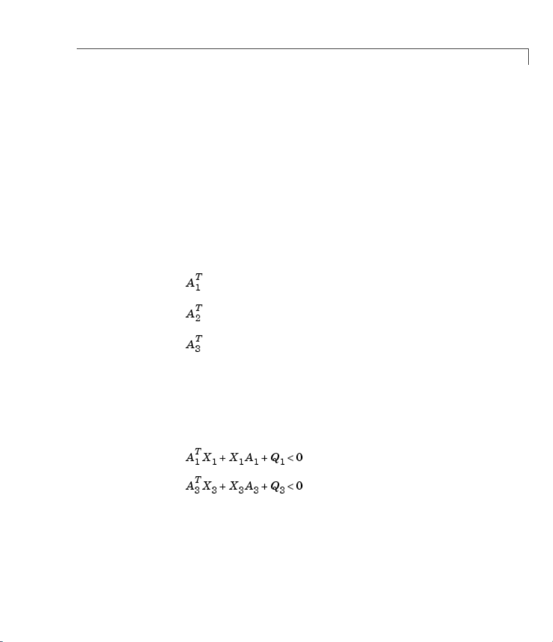
Examples Suppose that the three LMIs

X1+ X1A1+ Q

X2+ X2A2+ Q2<0

X3+ X3A3+ Q3<0

have be en declared in this order, labeled
andstoredin

lmis =

lmis

now describes the system of LMIs

lmisys. To delete the second LMI, type

dellmi(lmisys,LMI2)

1

<0

newlmi. Since this

LMI1, LMI2, LMI3 with newlmi,

d the second variable X

an

longer appears in the system.

no

has been removed from the problem since it

2

2-41

dellmi

See Also newlmi

To further delete LMI3 from the system, type

lmis = dellmi(lmis,LMI3)

or equivalently

lmis = dellmi(lmis,3)

Note that the system h as retained its original ranking after the first
deletion.

lmiedit

lmiinfo

2-42

delmvar

Purpose Remove one matrix variable from LMI problem

Syntax newsys = delmvar(lmisys,X)

Description delmvar removes the matrix variable X wi th identifier X from the list

of variables defined in
argument returned by
are automatically removed from the list of LMI terms. The description
of the resulting system of LMIs is returned in

Examples Consider the LMI

lmisys.TheidentifierX should be the second

lmivar when declaring X. All terms involving X

newsys.

involving
variable

lmisys = delmvar(lmisys,X)

Now lmis

with only one variable Y.NotethatY is still identified by the label Y.

See Also lmivar

setmvar

lmiinfo

two variables X and Y with identifiers

X,type

ys

describes the LMI

X and Y. To delete the

2-43

diag

Purpose Diagonalize vector of uncertain matrices and systems

Syntax v = diag(x)

Description If x is a vector of uncertain system models or matrices, diag(x) puts x

on the main diagonal. If x is a matrix of unc ertain system models or
matrices,
diagonal matrix of uncertain system models or matrices.

Examples The statement produces a diagonal system mxg of size 4-by-4. G iv en

multivariable system
found using

x = rss(3,4,1);
xg = frd(x,logspace(-2,2,80));
size(xg)

FRD model with 4 output(s) and 1 input(s), at 80 frequency point(s).

diag(x) is the main diagonal of x. diag(diag(x)) is a

xx, a vector of the diagonal elements of xxg is

diag.

See Also append

2-44

mxg = diag(xg);
size(mxg)
FRD model with 4 output(s) and 4 input(s), at 80 frequency point(s).

xxg = [xg(1:2,1) xg(3:4,1)];
m = diag(xxg);
size(m)
FRD model with 2 output(s) and 1 input(s), at 80 frequency point(s).

dkitopt

Purpose Create options o bject for use w ith dksyn

Syntax opt = dkitopt

opt = dkitopt('name1',value1,'name2',value2,...)

Description opt=dkitopt creates an options object opt of class dkitopt,usedto

define user-specified options in the µ-synthesis command
properties of

opt = dkitopt('name1',value1,'name2',value2,...) accepts

inputsasoneormoreProperty/Valuepairs to set user-specified values
of individual properties of
case-insensitive, and only enough characters to uniquely specify the
property name are required.

opt are set to their default values.

opt. Property names specification is not

dksyn.All

This table lists the

Object Property Description

FrequencyVector

InitialController

AutoIter

DisplayWhileAutoIter

StartingIterationNumber

NumberOfAutoIterations

MixedMU

dkitopt object properties.

Frequency vector used for analysis. Default is an
empty matrix ([]) which results in the frequency range
and number of points chosen automatically.

Controller used to initiate first iteration. Default is
an empty SS object.

Automated µ-synthesis mode. Default is 'on'.

Displays iteration progress in AutoIter mode. Default
is

'off'.

Starting iteration number. Default is 1.

Number of D-K iterations to perform. Default is 10.

Accounts for real-valued uncertain parameters for
µ-synthesis. For systems with atleast one real-valued
uncertain parameter, closed-loop robust performance
may improve when the option is set to
is

'off'.

'on'. Default

2-45

dkitopt

Object Property Description

AutoScalingOrder

AutoIterSmartTerminate

AutoIterSmartTerminateTol

Default

Meaning

If the AutoIter property is set to 'off', the D-K iteration procedure
is interactive. You are prompted to fit the D-Scale data and provide
input on the control design process.

If the

AutoIterSmartTerminate property is on, and a stopping criteria

(described below) is satisfied, the iteration performed by
will terminate before reaching the specified number of automated
iterations (value of
involves the objective value (peak value, across frequency, of the
upper bound for µ) in the current iteration, denoted v
the previous two iterations, (denoted v

AutoIterSmartTerminateTol.If

State order for fitting D-scaling and G-scaling data for
real or complex µ-synthesis. Defau lt is [5 2], 5th order
D-scalings and 2 nd order G-scaling s.

Automatic termination of iteration procedure based on
progress of design iteration. Default is

'on'.

Tolerance used by AutoIterSmartTerminate.Default
is 0.005.

Structure of property default values.

Structure text description of each property.

dksyn

NumberOfAutoIterations). The stopping criteria

,aswellas

and v-2) and the value of

-1

0

2-46

and

then the stopping criteria is satisfied (for lack of progress). The stopping
criteria is also satisfied if

which captures a significant increase (undesirable) in the objective.

dkitopt

Examples This example creates a dkitopt options object called opt with default

property values.

opt = dkitopt
Property Object Values:

FrequencyVector: []

InitialController: [0x0 ss]

AutoIter: 'on'

DisplayWhileAutoIter: 'off'

StartingIterationNumber: 1

NumberOfAutoIterations: 10

MixedMU: 'off'

AutoScalingOrder: [5 2]

AutoIterSmartTerminate: 'on'

AutoIterSmartTerminateTol: 0.0050

Default: [1x1 struct]
Meaning: [1x1 struct]

The properties can be modified directly with assignment statements:
here user-specified values for the frequency vector, the number of
iterations, and the maximum state dimension of th e D-scale fittings
are set.

opt.FrequencyVector = logspace(-2,3,80);
opt.NumberOfAutoIterations = 16;
opt.AutoScalingOrder = 16;
opt
Property Object Values:

FrequencyVector: [1x80 double]

InitialController: [0x0 ss]

AutoIter: 'on'

DisplayWhileAutoIter: 'off'

StartingIterationNumber: 1

NumberOfAutoIterations: 16

MixedMU: 'off'

AutoScalingOrder: 16

2-47

dkitopt

AutoIterSmartTerminate: 'on'

AutoIterSmartTerminateTol: 0.0050

Default: [1x1 struct]
Meaning: [1x1 struct]

Thesameproperty/valuepairsmaybesetwithasinglecalltodkitopt.

opt = dkitopt('FrequencyVector',logspace(-2,3,80),...

'NumberOfAutoIterations',16,...
'AutoScalingOrder',9);

Algorithm The dksyn command stops iterating before the total number

of automated iterations (

'AutoIterSmartTerminate' is set t o 'on' and a stopping criterion

is satisfied. The stopping criterion involves the m(i)valueofthe
current ith iteration,
and the options property
D-K iteration procedure automatically terminates if the difference
between each of the three µ values is less than the relative tolerance
of

AutoIterSmartTerminateTol xµ(i) or the current µ value µ(i)has

increased relative to the µ value of the previous iteration µ(i-1) by
20x

AutoIterSmartTerminateTol.

'NumberOfAutoIterations')if

m(i-1) and m(i-2), the previous two iterations

'AutoIterSmartTerminateTol'.The

See Also dksyn

2-48

When the system contains some real-valued uncertain parameters and

MixedMU is set to 'on', the dksyn command takes into account that

the uncertain parameters are real and this may result in improved
robust performance.

h2syn

hinfsyn

mussv

robopt

robuststab

robustperf

wcgopt

Tutorials Control of Spring-Mass-Damper Using Mixed mu-Synthesis

dkitopt

2-49

dksyn

Purpose Robust controller design using µ-synthesis

Syntax [k,clp,bnd] = dksyn(p,nmeas,ncont)

[k,clp,bnd] = dksyn(p,nmeas,ncont,opt)
[k,clp,bnd,dkinfo] = dksyn(p,nmeas,ncont,...)
[k,clp,bnd,dkinfo] = dksyn(p,nmeas,ncont,prevdkinfo,opt)
[...] = dksyn(p)

Description [k,clp,bnd] = dksyn(p,nmeas,ncont) synthesizes a robust controller

k for the uncertain open-loop plant model p via the D-K or D-G-K

algorithm for µ-synthesis.
The last

nmeas outputs and ncont inputs of p areassumedtobethe

measurement and control channels.
closed-loop m odel and

p, k, clp,andbnd are related as follows:

clp = lft(p,k);
bnd1 = robustperf(clp);
bnd = 1/bnd.LowerBound

p is an uncertain state space uss model.

k is the controller, clp is the

bnd is the robust closed-loop performance bound.

2-50

[k,clp,bnd] = dksyn(p,nmeas,ncont,opt) specifies user-defined

options

k,clp,bnd,dkinfo] = dksyn(p,nmeas,ncont,...) returns a log of the

[

algorithm execution in
N is the total number of iterations performed. The

opt for the D-K or D-K-G algorithm. Use dkitopt to create opt.

dkinfo. dkinfo is an N-by-1 cell array where

ith cell contains a

structure with the follow ing fields:

Field Description

K

Bnds

DL

DR

Controller at ith iteration, a ss object

Robust performance bound on the closed-loop
system (

double)

Left D-scale, an ss object

Right D -scale, an ss object

dksyn

Field Description

GM

GR

GFC

MussvBnds

MussvInfo

[k,clp,bnd,dkinfo] = dksyn(p,nmeas,ncont,prevdkinfo,opt)
allows you to use information from a previous dksyn
iteration. prevdkinfo

designing a robust controller using

dksyn starting iteration is not 1 (opt.StartingIterationNumber = 1)

to determ ine the correct D-scalings to initiate the iteration procedure.

[...] = dksyn(p) takes p as a uss object that has

two-input/two-output partitioning as defined by

Offset G-scale, an ss object

Right G -scale, an ss object

Center G-scale, an ss object

Upper and lower µ bounds, an frd object

Structure returned from mussv at each iteration.

is a structure from a previous attempt at

dksyn. prevdkinfo is used when the

mktito.

Examples The following statements create a robust performance control design

for an unstable, uncertain single-input/single-output plant model. The

nominal plant model, G, is an unstable first order system

G = tf(1,[1 -1]);

The model itself is uncertain. At low frequency, below 2 rad/s, it can
vary up to 25% from its nominal value. Around 2 rad/s the percentage
variation starts to increase a nd reaches 400% at approximately 32 rad/s.
The percentage model uncertainty is represented by the weight
which corresponds to the frequency variation of the model uncertainty
and the uncertain LTI dynamic object

Wu = 0.25*tf([1/2 1],[1/32 1]);
InputUnc = ultidyn('InputUnc',[1 1]);

InputUnc.

.

Wu

2-51

dksyn

The uncertain plant model Gpert represents the model of the physical
system to be controlled.

Gpert = G*(1+InputUnc*Wu);

The robust stability objectiveistosynthesizeastabilizingLTIcontroller
for all the plant models parameterized by the uncertain plant model,

Gpert. The performance objective is defined as a weighted sensitivity

minimization problem. The control interconnection structure is shown
in the following figure.

2-52

The sensitivity function, S, is defined as where P is the
plant model and
problem selects a weight
desired sensitivity function of th e closed-loop system as a function of
frequency. Hence the product of the sensitivity weight
closed-loop sensitivity function is less than 1 across all frequencies.
The sensitivity weight
decrease at 0.006 rad/s, and reaches a minimum magnitude of 0.25
after 2.4 rad/s.

Wp = tf([1/4 0.6],[1 0.006]);

The defined sensitivity weight Wp implies that the desired disturbance
rejection should be at least 100:1 dis turbance rejection at DC, rise

K is the controller. A weighted sensitivity minimization

Wp, which corresponds to the inverse of the

Wp and actual

Wp has a gain of 100 at low frequency, begins to

dksyn

slowly between 0.006 and 2.4 rad/s, and allow the disturbance rejection
to increase above the open-loop level, 0.25, at high frequency.

When the plant model is uncertain, the closed-loop performance
objective is to achieve the desired sensitivity function for all plant
models defined by the uncertain plant model,
objective for an uncertain system is a robust performance objective.
A block diagram of this uncertain closed-loop system illustrating the
performance objective (closed-loop transfer function from d→e )isshown.

From the definition of the robust performance control objectiv e, the
weighted, uncertain control design interconnection model, which
includes the robustness and performance objectives, can be constructed
and is denoted by

P. The robustness and performance weights are

selected such that if the robust performance structure singular value,

bnd, of the closed-loop uncertain system, clp, is less than 1 then the

performance objectives have been achieved for all the plant models in
the model set.

Gpert. T he performance

You can form the uncertain transfer matrix
using the following commands.

P = [Wp; 1 ]*[1 Gpert];
[K,clp,bnd] = dksyn(P,1,1);
bnd
bnd =

0.6819

P from [d; u] to [e; y]

2-53

dksyn

The controller K achieves a robust performance µ value bnd of 0.6819.
Therefore you have achieved the robust performance objectives for the
given problem.

You can use the
performance of

[rpnorm,wcf,wcu,report] = robustperf(clp);
disp(report{1})
Uncertain system, clp, achieves robust performance.
The analysis showed clp can tolerate 146% of the model uncertainty
and achieve the performance and stability objectives.
A model uncertainty exists of size 146% that results in
a peak gain performance of 0.686 at 0.569 rad/s.

robustperf command to analyze the closed-loop robust

clp.

Algorithm dksyn synthesizes a robust controller via D-K iteration. The D-K

iteration procedure is an approximation to µ-synthesis control design.
The objective of µ-synthesis is to minimize the structure singular
value µ of the corresponding robust performance problem associated
with the uncertain system
interconnection containing known components including the nominal
plant model, uncertain parameters,
dynamics,

ultidyn, and performance and uncertainty weighting

functions. You use weighting functions to include magnitude and
frequency shaping information in the optimization. The control
objectiveistosynthesizeastabilizingcontroller
robust performance µ value, which corresponds to

The D-K iteration procedure involves a sequence of minimizations, first
over the controller variable K (holding the D variable associated with
the scaled µ upper bound fixed), and then over the D variable (holding
the controller K variable fixed). The D-K iteration procedure is not
guaranteed to converge to the minimum µ value, but often works well
in practice.

p. The uncertain system p is an open-loop

ucomplex, and unmodeled LTI

k that minimizes the

bnd.

2-54

dksyn automates the D-K iteration procedure and the options object
dkitopt allows you to customize its behavior. Internally, the algorithm

dksyn

works with the generalized scaled plant model P, which is extracted
from a

The following is a list of what occurs during a single, complete step
of the D-K iteration.

1 (In the first iteration, this step is skipped.) The µ calculation (from

uss object using the command lftdata.

the previous step) provides a frequency-dependent scaling matrix, D
The fitting procedure fits these scalings with rational, stable transfer
function matrices. After fitting, plots of

and

are shown for comparison.

.

f

(In the first iteration, this ste p is skipp ed.) The rational

is
absorbed into the open-loop interconnection for the nex t controller
synthesis. Using either the previous frequency-dependent D’sor
the just-fit rational

,anestimateofanappropriatevalueforthe
H∞norm is made. This is simply a conservative value of the scaled
closed-loop H

norm, using the most recent controller and either a

∞

frequency sweep (using the frequency-dependent D’s) or a state-space
calculation (with the rational D’s).

2 (The first iteration begins at this point.) A controller is designed

using H
the

synthesis on the scaled open-loop interconnection. If you set

∞

DisplayWhileAutoIter field in dkitopt to 'on', the following

information is displayed:

a The progress of the γ-iteration is displayed.

b The singular values of the closed-loop frequency response are

plotted.

2-55

dksyn

c You are given the option to change the frequency range. If you

change it, all relevant frequency responses are automatically
recomputed.

d You are given the option to rerun the H

modified parameters if you set the

'off'. This is convenient if, for instance, the bisection tolerance

was too large, or if

3 The structured singular value of the closed-loop system is calculated

maximum gamma value was too small.

synthesis with a set of

∞

AutoIter field in dkitopt to

and plotted.

4 An iteration summary is displayed, showing all the controller order,

as well as the peak value of µ of the closed-loop frequency responses.

5 The choic e of stopping or performing another iteration is given.

Subsequent iterations proceed along the same lines without the need to
reenter the iteration number. A summary at the end of each iteration is
updated to reflect data from all previous iterations. This often provides
valuable information about the progress of the robust controller
synthesis procedure.

Interactive Fitting of D-Scalings

Setting the AutoIter field in dkitopt to 'off' requires that you
interactively fit the D-scales each iteration. During step 2 of the D-K
iteration procedure, you are prompted to enter y our choice of options
for f itting the D-scaling data. You press return after, the following is a
list of your options.

2-56

Enter Choice (return for list):
Choices:
nd Move to Next D-Scaling
nb Move to Next D-Block

i Increment Fit Order
d Decrement Fit Order
apf Auto-PreFit

dksyn

mx 3 Change Max-Order to 3
at 1.01 Change Auto-PreFit tol to 1.01
0 Fit with zeroth order
2 Fit with second order
n Fit with n'th order
e Exit with Current Fittings
s See Status

• nd and nb allow you to move from one D-scale data to another. nd

moves to the next scaling, whereas nb moves to the next scaling block.
For scalar D-scalings, these are identical operations, but for problems
with full D-scalings, (perturbations of the form δI) they are different.
In the (1,2) subplot w indow, the title displays the D-scaling block
number, the row/column o f the scaling that is currently being fitted,
and the order of the current fit (with

• Y ou can increment or decrement the order of the current fit (by 1)

using

i and d.

apf automatically fits each D-scaling data. The default maximum

•

state order of individual D-scaling is 5. The
to change the maximum D-scaling state order used in the automatic
prefitting routine.

mx must be a positive, nonzero integer. at allows

you to define how close the rational, scaled µ upper bound is to
approximate the actual µ upper bound in a norm sense. Setting

1 would require an exact fit of the D-scale data, and is not allowed.

Allowable values for

at are greater than 1. This setting plays a role

(mildly unpredictable, unfortunately) in determining where in the
(D,K)spacetheD-K iteration converges.

d fo r data when no fit exists).

mx variable allows you

at to

• E n tering a positive integer at the prompt will fit the current D-scale

data with that state order rational transfer function.

•

e exits the D-scale fitting to continue the D-K iteration.

• The variable

s displays a status of the current and fits.

Limitations There are two shortcomings of the D-K iteration control design

procedure:

2-57

dksyn

• Calculation of the structured singular value µΔ(·) is approximated by

its upper bound. This is not a serious problem because the value of µ
and its upper bound are often close.

• The D-K iteration is not guaranteed to converge to a glo bal, or even

local minimum. This is a serious problem, and re pre sents the biggest
limitation of the design procedure.

In spite of these drawbacks, the D-K iteration control design technique
appears to work well on many engineering problems. It has been
applied to a number of real-world applications with success. These
applications include vibration suppressio n for flexible structures, flight
control, chemical process control problems, and acoustic reverberation
suppression in enclosures.

References • Balas, G.J., and J.C. Doyle, “Robust control of flexible modes in the

controller crossover region,” AIAA Journal of Guidance, Dynamics
and Control, Vol. 17, no. 2, March-April, 1994, p. 370-377.

• Balas, G.J., A.K. Packard, and J.T. Harduvel, “Application of

µ-synthesis techniques to momentum management and attitude
control of the space station,” AIAA Guidance, Navigation and Control
Conference, New Orleans, August 1991.

See Also dkitopt

2-58

• D oy le, J.C., K. Lenz, and A. Packard, “Design examples using

µ-synthesis: Space shuttle lateral axis FCS during reentry,” NATO
ASI Series, Modelling, Robustne ss, and Sensitivity Reduction in
Control Systems, vol. 34, Springer-Verlag, Berlin 1987.

• P ackard, A., J. Doyle, and G. Balas, “Linear, multivariable robust

control w ith a µ perspective,” ASME Journal of Dynamic Systems,
Measurement and Control, 50th Anniversary Issue, Vol. 115, no.
2b, June 1993, p. 310-319.

• Stein, G., and J. Doyle, “Beyond singular values and loopshapes,”

AIAA Journal of Guidance and Control,Vol.14,No.1,January,
1991, p. 5-16.

h2syn

hinfsyn

Comprehensive analysis of feedback loop

mktito

mussv

robuststab

robustperf

wcgain

wcsens

wcmargin

Tutorials Control of Spring-Mass-Damper Using Mixed mu-Synthesis

dksyn

2-59

dmplot

Purpose Interpret disk g ain and phase margins

Syntax dmplot

dmplot(diskgm)

[dgm,dpm] = dmplot

Description dmplot plots disk gain margin (dgm) and disk phase margin (dpm). Both

margins are derived from the largest disk that

• Contains the critical point (-1,0)

• Does not intersect the Nyquist plot of the open-loop response L

diskgm is the radius of this disk and a lower bound on the classical

gain margin.

dmplot(diskgm) plots the maximum allowable phase variation as a

function o f the actual gain variation for a given disk gain margin
(the maximum gain variation being diskgm). The c lo sed-loop system
is guaranteed to remain stable for all combined gain/phase variations
inside the plotted ellipse.

diskgm

[dgm,dpm] = dmplot returns the data used to plot the gain/phase

variation ellipse.

Examples When you call dmplot (without an argument), the resulting plot shows a

comparison of a disk margin analysis w ith the classical notations of gain
and phase margins. The Nyquist plot is of the loop transfer function L(s)

• The Nyquist plot of L corresponds to the blue line.

• T he unit disk corresponds to the dotted red line.

2-60

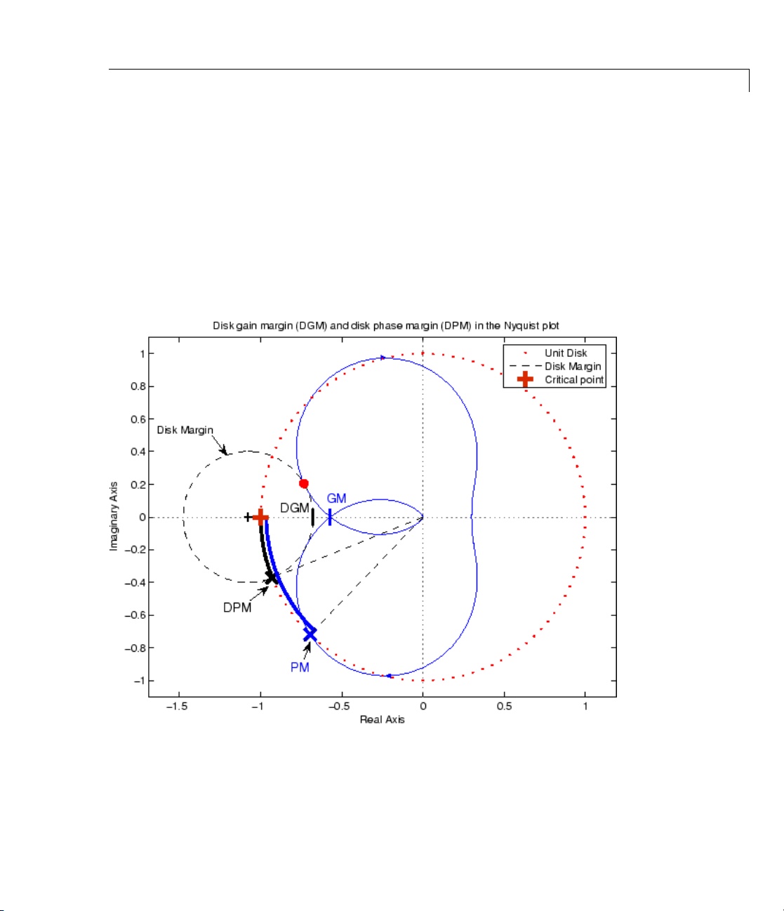
dmplot

• GMandPMindicatethelocationof the classical gain and phase

margins for the system L.

• D G M and DPM correspond to the disk gain and phase margins,

respectively. The disk margins provide a lower bound on classical
gain and phase margins.

• The disk margin circle, represented by the dashed black line,

corresponds to the largest disk centered at
just touches the loop transfer function L. This location is indicated
by the red dot.

(DGM + 1/DGM)/2 that

2-61

dmplot

The x-axis corresponds to the gain variation, in dB, and the y-axis
corresponds to the phase variation allowable, in degrees. For a disk
gain margin corresponding to 3 dB (1.414), the closed-loop system is
stable for all phase and gain variations inside the blue ellipse. For
example, the closed-loop system can simultane ously tolerate +/- 2 dB
gain variation and +/- 14 deg phase variations.

dmplot(1.414)

2-62

dmplot

References Barrett, M.F., Conservatism with robustness tests for linear feedback

control systems, Ph.D. Thesis, Control Science and Dynamical Systems,
University of Minnesota, 1980.

Blight, J.D., R.L. Dailey, and Gangsass, D., “Practical control law design
for aircraft using multivariable techniques,” International Journal of
Control, Vol. 59, No. 1, 1994, 93-137.

Bates, D., and I. Postlethwaite, Robust Multivariable Control of
Aerospace Systems, Delft University Press, Delft, The Netherlands,
ISBN: 90-407-2317-6, 2002.

See Also Comprehensive stability analysis of feedback loops

wcmargin

2-63

drawmag

Purpose Mouse-based tool for sketching and fitting

Syntax [sysout,pts] = drawmag(data)

[sysout,pts] = drawmag(data,init_pts)

Description drawmag interactively uses the mouse in the plot window to create pts

(the frd object) and sysout (a stable minimum-phase ss object), which
approximately fits the frequency response (magnitude) in

Input arguments:

pts.

data

init_pts

Output arguments:

sysout

pts

While

drawmag is running, all interaction with the program is through

the mouse and/or the keyboard. The mouse, if there is one, must be in
the plot window. The program recognizes several commands:

• C licking the mouse button adds a point at the cross-hairs. If the

cross-hairs are outside the plotting window, the points are plotted
when the fitting, windowing, or replotting mode is invoked. Typing

a is the same as clicking the mouse button.

• Typing

cross-hairs.

• Typing any integer between

transfer function of that order. The fitting routine a pproximately

Either a frequency response object that is plotted
as a reference, or a constant matrix of the form
[x

minxmaxyminymax

data.

Optional frd objectsofinitialsetofpoints

Stable, minimum-phase ss object that approximately
fits, in magnitude, the

Frequency response of points.

r removes the point with frequency nearest that of the

] specifying the plot window on the

pts data.

0 and 9 fits the existing points with a

2-64

drawmag

minimizes the maximum error in a log sense. The new fit is displayed
along with the po ints, and the most recent previous fit, if it exists.

• Typing

window. M oving the cross-hairs and clicking the mouse or pressing
any key then gives a second point at the new cross-hair location.
These two points define a new window on the data, which is
immediately replotted. This is useful in fine tuning parts of the data.
You can call windowing repeatedly.

• Typing

current data points as well as w hatever was specified in
used after windowing to view all the data.

• Typing

should exercis e caution when using this option, as it can wreak havoc
on the program if variables are changed.

See Also ginput

loglog

w uses the cross-hair location as the initial point in creating a

p simply replots the data using a window that covers all the

in.Typically

k invokes the keyboard using the keyboard command. You

2-65

evallmi

Purpose Given particular instance of decision variables, evaluate all variable

terms in system of LMIs

Syntax evalsys = evallmi(lmisys,decvars)

Description evallmi evaluates all LMI constraints for a particular instance decvars

of the vector of decision variables. Recall that decvars fully determines
the values of the matrix variables X
of replacing all terms involving X
output

evalsys is an LMI system containing only constant terms.

,.. .,XK. The “evaluation” consists

1

,.. .,XKby their matrix value. The

1

The function
The vector returned by these solvers can be fed directly to

evallmi is useful for validation of the LMI solvers’ output.

evallmi

to evaluate all variable terms. The matrix values of the left- and
right-hand sides of each LMI are then returned by

showlmi.

Observation evallmi is meant to operate on the output of the LMI solvers. To

evaluate all LMIs for particular instances of the matrix variables X
., X

, first form the corresponding decision vector x with mat2dec and

K

then call

evallmi with x as input.

Examples Consider the feasibility problem of finding X >0suchthat

T

A

XA – X + I <0

where

setlmis([])
X = lmivar(1,[2 1]) % full symmetric X

lmiterm([1 1 1 X],A',A) % LMI #1: A'*X*A
lmiterm([1 1 1 X],-1,1) % LMI #1: -X
lmiterm([1 1 1 0],1) % LMI #1: I
lmiterm([-2 1 1 X],1,1) % LMI #2: X
lmis = getlmis

This LM I system is defined by:

,..

1

2-66

evallmi

To compute a solution xfeas,callfeasp by

[tmin,xfeas] = feasp(lmis)

The result is

tmin =

-4.7117e+00

xfeas' =

1.1029e+02 -1.1519e+01 1.1942e+02

The LMI constraints are therefore feasible since tmin <0. Thesolution
X corresponding to the feasible decision vector
by

X = dec2mat(lmis,xfeas,X).

xfeas would be given

To check that

xfeas is ind eed feasible, evaluate all LMI constraints

by typing

evals = evallmi(lmis,xfeas)

The left- and right-hand sides of the first and second LMIs are then
given by

[lhs1,rhs1] = showlmi(evals,1)
[lhs2,rhs2] = showlmi(evals,2)

and the test

eig(lhs1-rhs1)
ans =

-8.2229e+01

-5.8163e+01

confirms that the first LMI constraint is satisfied by xfeas.

2-67

evallmi

See Also showlmi

setmvar

dec2mat

mat2dec

2-68

feasp

Purpose Compute solution to given system of LMIs

Syntax [tmin,xfeas] = feasp(lmisys,options,target)

Description The function feasp computes a solution xfeas (ifany)ofthesystemof

LMIs des cribed by
decision variables for which all LMIs are satisfied.

Given the LMI system

lmisys.Thevectorxfeas is a particular value of the

(2-3)

rol

Cont
Parameters

xfeas is com

Minimize t subject to

The global minimum of this program is the scalar value tmin returned
as first output argument by

tmin ≤ 0 and strictly feasible if tmin < 0. If the problem is feasible but

not strictly feasible,
maythenberequiredtodecidewhether
feasible.

The optional argument
optimization code terminates as soon as a value of t below this target is
reached. The default value is

Note that
in terms of the matrix variables of the problem. Use
feasible values of the matrix variables from

ptional argument

The o

meters for the optimization algorithm. This five-entry vector is

para

nized as follows:

orga

ions(1)

•

opt

ions(2)

•

opt

formed by the optimization procedure (100 by default).

per

puted by solving the auxiliary convex program:

feasp. The LMI constraints are feasible if

tmin is positive and very small. Some post-analysis

xfeas is close enough to

target sets a target value for tmin.The

target =0.

xfeas is a solution in terms of the decision variables and not

dec2mat to derive

xfeas.

options gives access to certain control

is not used.

sets the maximum number of iterations allowed to be

2-69

feasp

• options(3) resets the feasibility radius.Settingoptions(3) to a

value R > 0 further constrains the decision vector x =(x

,.. .,xN)to

1

lie within the ball

In other words, the Euclidean norm of xfeas should not exceed R.The
feasibility radius is a simple means of controlling the magnitude of
solutions. Upon termination,

feasp displays the f-radius saturation,

that is, the norm of the solution as a percentage of the feasibility
radius R.

The default value is R = 109. Setting

options(3) to a neg ative value

activates the “flexible bound” m ode. In this mode, the feasibility
radius is initially set to 108, and increased if necessary during the
course of optimization

•

options(4) helps speed up termination. When set to an integer

value J > 0, the code terminates if t did not decrease by more than
one percent in relative terms during the last J iterations. The default
value is 10. This p arameter trades off speed vs. accuracy. If set to a
small value (< 10), the code term inates quickly but without guarantee
of accuracy. On the contrary, a large value results in natural
convergence at the expense of a possibly large number of iterations.

•

options(5) = 1 turns off the trace of exec ution of the optimization

procedure. Resetting

options(5) to zero (default value) turns it

back on.

Setting

option(i) to zero is equivalent to setting the corresponding

control parameter to its default value. Consequently, there is no need to
redefine the entire vector when changing just one control parameter.
To set the maximum number of iterations to 10, for instance, it suffices
to type

options=zeros(1,5) % default value for all parameters
options(2)=10

2-70

feasp

Memory
Problems

When the least-squares problem solved at each iteration becomes
ill conditioned, the
QR-based linear algebra (see “Memory Problems” on page 2-2 10 for
details). Since the QR mode typically requires much more memory,
MATLAB may run out of memory and display the message

??? Error using ==> feaslv
Out of memory. Type HELP MEMORY for your options.

You should then ask your system man ag er to increase your swap space
or, i f no additional swap space is available, set
will prevent switching to QR and
fails due to numerical instabilities.

feasp solver switches from Cholesky-based to

feasp will terminate w hen Cholesky

Examples Consider the problem of finding P > I such that

with data

options(4) = 1.This

(2-4)

(2-5)

(2-6)

This problem arises when studying the quadratic stability of the
polytope of matrices Co{A

To assess feasibility with

-Equation2-6:

setlmis([])
p = lmivar(1,[2 1])

, A2, A3}.

1

feasp, first enter the LMIs Equation 2-4

2-71

feasp

lmiterm([1 1 1 p],1,a1,'s') % LMI #1
lmiterm([2 1 1 p],1,a2,'s') % LMI #2
lmiterm([3 1 1 p],1,a3,'s') % LMI #3
lmiterm([-4 1 1 p],1,1) % LMI #4: P
lmiterm([4 1 1 0],1) % LMI #4: I
lmis = getlmis

Then call feasp to find a feasible decision vector:

[tmin,xfeas] = feasp(lmis)

This returns tmin = -3.1363. Hence Equation 2-4 - Equation 2-6 is
feasible and the dynamical system
A(t)

Co{A1, A2, A3}.

= A(t)x is quadratically stable for

To obtain a Lyapunov matrix P proving the quadratic stability, type

P = dec2mat(lmis,xfeas,p)

This returns

It is possible to add further constraints on this feasibility problem. For
instance, you can bound the Frobenius norm of P by 10 while asking

tmin to be less than or equal to –1. This is done by

[tmin,xfeas] = feasp(lmis,[0,0,10,0,0],-1)

The third entry 10 of options sets the feasibility radius to 10 while the
third argument

-1.1745

and a matrix P with largest eigenvalue λ

-1 sets the target value for tmin. This yields tmin =

(P) = 9.6912.

max

References The feasibility solver feasp is based on Nesterov and N e m iro vski’s

Projective Method described in

2-72

feasp

Nesterov, Y., and A. Nemirovski, Interior Point Polynomial Methods in
Convex Programming: Theory and Applications,SIAM,Philadelphia,

1994.

Nemirovski, A ., and P. Gahinet, “The Projective Method for Solving
Linear Matrix Inequalities,” Proc. Amer. Contr. Conf., 1994, Baltimore,
Maryland, p. 840–844.

The optimization is p erformed by the C-MEX file

See Also mincx

gevp

dec2mat

feaslv.mex.

2-73

fitfrd

Purpose Fit frequency response data with state-space model

Syntax B = fitfrd(A,N)

B = fitfrd(A,N,RD)
B = fitfrd(A,N,RD,WT)

Description B = fitfrd(A,N) is a state-space object w ith state dimension N, wh ere

A is an frd object and N is a nonnegative integer. The frequency

response of

A must have either 1 row or 1 column, although it need not be 1-by-1. B

willbethesamesizeasA.Inallcases,N should be a nonnegative scalar.

B = fitfrd(A,N,RD) forces the relative degree of B to be RD. RD must be

a nonnegative integer. The default value for
column) then
relative degree of each entry of
relative degree for all entries of

RD by setting RD to an empty matrix.

B = fitfrd(A,N,RD,WT) uses the magnitude of WT to weight the

optimization fit criteria.
scalar, then it is used to weight all entries of the error criteria (

WT is a vector, it must be the same size as A, and each individual entry

of

WT acts as a weighting function on the corresponding entry of (A-B).

B closely matches the D-scale frequency response data in A.

RD is 0. If A is a row (or

RD canbeavectorofthesamesizeaswell,specifyingthe

B.IfRD is a scalar, then it specifies the

B. You can specify the d efault value for

WT can be a double, ss or frd.IfWT is a

A-B). If

Examples You can use the fitfrd command to fit D-scale data. For example,

create D -scale frequency response data from a fifth-order system.

sys = tf([1 2 2],[1 2.5 1.5])*tf(1,[1 0.1]);
sys = sys*tf([1 3.75 3.5],[1 2.5 13]);
omeg = logspace(-1,1);
sysg = frd(sys,omeg);
bode(sysg,'r-');

2-74

You can try to fit the frequency response D-scale data sysg with a
first-order system,
a third-order system,

b1. Similarly, you can fit the D- scale data with

b3.

fitfrd

b1 = fitfrd(sysg,1);
b3 = fitfrd(sysg,3);

Compare the original D-scale data sysg with the frequency responses of
the first and third-order models calculated by

b1g = frd(b1,omeg);
b3g = frd(b3,omeg);
bode(sysg,'r-',b1g,'k:',b3g,'b-.')

fitfrd:

2-75

fitfrd

Limitations Numerical conditioning problems arise if the state order of the fit N is

selected to be higher than required by the dynamics of

A.

See Also fitmagfrd

2-76

fitmagfrd

Purpose Fit frequency response magnitude data with minimum-phase

state-space model using log-Chebychev magnitude design

Syntax B = fitmagfrd(A,N)

B = fitmagfrd(A,N,RD)
B = fitmagfrd(A,N,RD,WT)
B = fitmagfrd(A,N,RD,WT,C)

Description B = fitmagfrd(A,N) is a stable, minimum-phase ss object, with

state-dimension
matches the magnitude data in
nonnegative integer.

B = fitmagfrd(A,N,RD) forces the relative degree of B to be RD. RD

must be a nonnegative integer whose default value is 0. You can specify
the default value for

B = fitmagfrd(A,N,RD,WT) uses the magnitude of WT to weight the

optimization fit criteria.
then it is used to weight all entries of the error criteria
vector,itmustbethesamesizeas
as a weighting function on the corresponding entry of (
value for

WT is 1, and you can specify it by setting WT to an empty matrix.

N, whose frequency response magnitude closely

A. A is a 1-by-1 frd object, and N is a

RD by setting RD to an empty matrix.

WT can be a double, ss or frd.IfWT is a scalar,

(A-B).IfWT is a

A,andeachindividualentryofWT acts

A-B). The default

B = fitmagfrd(A,N,RD,WT,C) enforces additional magnitude

constraints on

C.UpperBound.Thesecanbeempty,double or frd (with C.Frequency

B,specifiedbythevaluesofC.LowerBound and

equal to A.Frequency). If C.LowerBound is non-empty, then the
magnitude of
bound is enforced at frequencies where
Similarly, the
on the magnitude of
to

A.Frequency), then the upper and lower bound constraints on B are

taken directly from

B is constrained to lie above C.LowerBound. No lower

C.LowerBound is equal to -inf.

UpperBound field can be used to specify an upper bound

B.IfC is a double or frd (with C.Frequency equal

A as:

• if C(w) == –1, then enforce abs(B(w)) <= abs(A(w))

• if C(w) == 1, then enforce abs(B(w)) >= abs(A(w))

2-77

fitmagfrd

• if C(w) == 0, then no additional constraint

where

w denotes the frequency.

Examples Fit frequency response magnitude data with a stable, min imum-phase

statespace model:

1 Create frequency response magnitude data from a fifth-order system.

sys = tf([1 2 2],[1 2.5 1.5])*tf(1,[1 0.1]);
sys = sys*tf([1 3.75 3.5],[1 2.5 13]);
omega = logspace(-1,1);
sysg = abs(frd(sys,omega));
bodemag(sysg,'r');

2-78

fitmagfrd

2 Fit the

syste

magnitude data with a minimum-phase, stable third-order

m:

ord = 3;
b1 = fitmagfrd(sysg,ord);
b1g = frd(b1,omega);
bodemag(sysg,'r',b1g,'k:');

2-79

fitmagfrd

2-80

3 Fit the

below

magnitude data with a third-order system constrained to lie

and above the given data.

C2.UpperBound = sysg;
C2.LowerBound = [];
b2 = fitmagfrd(sysg,ord,[],[],C2);
b2g = frd(b2,omega);
C3.UpperBound = [];
C3.LowerBound =sysg;
b3 = fitmagfrd(sysg,ord,[],[],C3);