Mathworks RF BLOCKSET 2 user guide

RF Blockset™ 2

User’s Guide

How to Contact The MathWorks

www.mathworks.
comp.soft-sys.matlab Newsgroup
www.mathworks.com/contact_TS.html Technical Support

[e-mail] Product enhancement suggestions

bugs@mathwo
[e-mail] Documentation error reports
[e-mail] Order status, license renewals, passcodes

info@mathwo

com

rks.com

rks.com

Web

Bug reports

Sales, prici

ng, and general information

508-647-7000 (Phone)

508-647-7001 (Fax)

The MathWorks, Inc.
3 Apple Hill Drive
Natick, MA 01760-2098

For contact information about worldwide offices, see the MathWorks Web site.

RF Blockset™ User’s Guide

© COPYRIGHT 2004–20 10 by The MathWorks, Inc.

The software described in this document is furnished under a license agreement. The software may be used
or copied only under the terms of the license agreement. No part of this manual may be photocopied or
reproduced in any form without prior written consent from The MathW orks, Inc.

FEDERAL ACQUISITION: This provision applies to all acquisitions of the Program and Documentation
by, for, or through the federal government of the United States. By accepting delivery of the Program
or Documentation, the government hereby agrees that this software or documentation qualifies as
commercial computer software or commercial computer software documentation as such terms are used
or defined in FAR 12.212, DFARS Part 227.72, and DFARS 252.227-7014. Accordingly, the terms and
conditions of this Agreement and only those rights specified in this Agreement, shall pertain to and govern
theuse,modification,reproduction,release,performance,display,anddisclosureoftheProgramand
Documentation by the federal government (or other entity acquiring for or through the federal government)
and shall supersede any conflicting contractual terms or conditions. If this License fails to meet the
government’s needs or is inconsistent in any respect with federal procurement law, the government agrees
to return the Program and Docu mentation, unused, to The MathWorks, Inc.

Trademarks

MATLAB and Simulink are registered trademarks of The MathWorks, Inc. See

www.mathworks.com/trademarks for a list of additional trademarks. Other product or brand

names may be trademarks or registered trademarks of their respective holders.

Patents

The MathWorks products are protected by one or more U.S. patents. Please see

www.mathworks.com/patents for more information.

Revision History

June 2004 Online only New for V ersion 1.0 (Release 14)
August 2004 Online only Revised for Version 1.0.1 (Release 14+)
March 2005 Online only Revised for Version 1.1 (Release 14SP2)
September 2005 Online only Revised for Version 1.2 (Release 14SP3)
March 2006 Online only Revised for Version 1.3 (Release 2006a)
September 2006 Online only Revised for Version 1.3.1 (Release 2006b)
March 2007 Online only Revised for Version 2.0 (Release 2007a)
September 2007 Online only Revised for Version 2.1 (Release 2007b)
March 2008 Online only Revised for Version 2.2 (Release 2008a)
October 2008 Online only Revised for Version 2.3 (Release 2008b)
March 2009 Online only Revised for Version 2.4 (Release 2009a)
September 2009 Online only Revised for Version 2.5 (Release 2009b)
March 2010 Online only Revised for Version 2.5.1 (Release 2010a)

Getting Started

1

Product Overview ................................. 1-2

Contents

Required and Related Products

Product Demos

RF Blockset Libraries

Overview o f RF Blockset Libraries
Opening RF Blockset Libraries
Physical Library
Mathematical Library

Product Workflow

Example — Modeling an LC Bandpass Filter

Overview o f LC Bandpass Filter Example
Selecting Blocks to Represent System Components
Building the Model
Specifying Model Parameters
Validating Filter Components and Running the

Simulation

Analyzing the Simulation Results

.................................... 1-4

.............................. 1-6

.................................. 1-7

.............................. 1-9

................................. 1-11

................................ 1-14

..................................... 1-23

..................... 1-3

................... 1-6

...................... 1-6

.............. 1-13

........................ 1-16

.................... 1-25

......... 1-13

...... 1-13

Modeling an RF System

2

Modeling RF Components .......................... 2-2

Adding RF Blocks to a Model
Connecting Model Blocks

........................ 2-2

........................... 2-3

v

Specifying or Importing Component Data ............ 2-7

Specifying Parameter Values
Supported File Types for Importing Data
Importing Data Fil es into RF Blocks
Example — Importing a Touchstone Data File into an RF

Model
Importing Circuits from the MATLAB Workspace
Example — Importing a Bandstop Filter into an RF

Model

......................................... 2-10

......................................... 2-14

........................ 2-7

.............. 2-7

.................. 2-8

....... 2-14

Specifying Operating Conditions

Modeling Nonlinearity

Amplifier and Mixer Nonlinearity Specifications
Adding Nonlinearity to Your System

Modeling Noise

Amplifier and Mixer Noise Specifications
Adding Noise to Your System
Plotting Noise

.................................... 2-26

.................................... 2-31

............................. 2-23

.................... 2-21

........ 2-23

.................. 2-24

.............. 2-26

........................ 2-27

Plotting Model Data

3

Creating Plots ..................................... 3-2

Available Data for Plotting
Using Plots to Validate Individual Blocks and

Subsystems
Types of Plots
Plot Formats
HowtoCreateaPlot
Example — Plotting Component Data on a Z Smith

Chart

.................................... 3-3

.................................... 3-3

..................................... 3-5

......................................... 3-22

.......................... 3-2

............................... 3-14

vi Contents

Updating Plots

Modifying Plots

.................................... 3-27

................................... 3-28

Example — Creating and Modifying Subsystem

Plots

Plotting the Network Parameters of a Subsystem
Adding Data to an Existing Plot
Changing Data on an Existing Plot

........................................... 3-31

....... 3-31

..................... 3-33

................... 3-35

Block Reference

4

Mathematical ..................................... 4-2

Physical

Ladder Filters
Series/Shunt RLC
Transmission Lines
Black Box Elements
Amplifiers
Mixers
Input/Output Ports

.......................................... 4-3

.................................... 4-3

................................. 4-3

................................ 4-4

............................... 4-4

....................................... 4-5

.......................................... 4-5

................................ 4-5

Blocks — Alphabetical List

5

RF Blockset Algorithms

A

Simulating an RF Model ............................ A-2

Determining the Modeling Frequencies

Mapping Network Parameters to Modeling

Frequencies

..................................... A-5

.............. A-3

vii

ModelingNoiseinanRFSystem .................... A-7

Output-Referred No ise in RF Models
Calculating Noise Figure at Modeling Frequencies
Calculating System Noise Figure
Calculating Output Noise Power

.................. A-7

...... A-10

..................... A-11

..................... A-12

Creating a Complex Baseband-Equivalent Model

Baseband-Equivalent Modeling
Simulation Efficiency of a Baseband-Equivalent Model
Example — Selecting Parameter Values for a

Baseband-Equivalent Model

Converting to and from Simulink Signals

Signal Conversion Specifications
Interpreting the Simulink Signal as the Incident Power

Wave
Interpreting the Simulink Signal as the Source Voltage
Specifying Input Signal Conversions

......................................... A-33

...................... A-13

...................... A-19

............ A-32

..................... A-32

.................. A-36

Modeling Mixers

B

2-Port Mixer Blocks ................................ B-2

Modeling a Mixer Chain

............................ B-4

..... A-13

... A-18

.. A-35

viii Contents

Quadrature Mixers

Using RF Blockset SoftwaretoModelQuadrature

Mixers
Modeling U pconv ersion I/Q Mixers
Modeling Do wnco nversion I/Q Mixers
Simulating I/Q Mixers

........................................ B-6

................................ B-6

................... B-6

................. B-7

............................. B-8

Examples

C

Examples ......................................... C-2

Index

ix

x Contents

Getting Started

• “Product Overview” on page 1-2

• “Required and Related Products” on page 1-3

• “Product Demos” on page 1-4

• “RF Blockset Libraries” on page 1-6

• “Product Workflow” on page 1-11

• “Example — Modeling an LC Bandpass Filter” on page 1-13

1

1 Getting Started

Product Overview

RF Blockset™ software extends your Simulink®modeling environment
with a library of blocks for modeling RF systems that include RF filters,
transmission lines, amplifiers, and mixers. For more information about
creating and running Simulink models, s ee “Creating a Simulink Model” in
the Simulink User’s Guide.

You use RF Blockset blocks to represent the components of your RF system
in a Simulink model. The blockset provides several types of compo nent
representations using network parameters (S, Y, Z, ABC D, H, and T format),
mathematical descriptions, and physical properties.

In the Simulink model, you cascade the components to represent your RF
architecture and run the simulation. During the simulation, the model
computes a time-domain, complex-baseband representation. This method
results in fast simulation of the quadrature modeling schemes used in modern
communication systems and enables compatibility with other Simulink blocks.

1-2

The blockset lets you visualize the network parameters of the blocks using
plots and Smith

A validated Simulink model of an RF system can provide an executable
specification for RF circuit design for wireless communication systems.

You can also use the blockset with Real-Time Workshop
embeddable C code for real-time execution.

®

Charts.

®

software to generate

Required and Related Products

In addition to MATLAB®and Simulink, you must have the following products
installed to use RF Blockset software:

• RF Toolbox™ — Provides MATLAB functions for defining, simulating, and

visualizing RF components.

• Signal Processing Toolbox™ — Provides MATLAB functions for filtering

wireless communication signals.

• Signal Processing Blockset™ — Provides Simulink blocks for time-domain

simulation of communication signals.

You can build sophisticated wireless communication system models by
incorporating blocks from other blocksets, such as Signal Processing Blockset
and Communications Blockset™ .

The MathWorks™ provides several products that are especially relevant to
the kinds of tasks you can perform with RF Blockset software. The following
table summarizes the related products and describes how they complement
the features of this product.

Required and Related Products

Product

Communications Blockset Simulink blocks for time-domain

Communications Toolbox™ MATLAB functions for signal

Filter Design Toolbox™

Descrip

simulation of modulation and
demodulation of a wireless
communications signal.

modulation and demodulation.

MATLAB functions for filtering the
modulated comm unication signal.

tion

1-3

1 Getting Started

Product Demos

You can find interactive RF Blockset d emo s in the MATLAB Help browser, as
shown in the following figure.

1-4

To open the RF Blockset Demos page in the Help Browser:

• Type demo 'blockset' 'rf' at the MATLAB prompt.

• Expand the RF Blockset section and click Demos.

To run an demo:

1 Browse to demo you want to run.

2 Onthedemopage,clickRunintheCommandWindowin the

upper-right corner of the demo window.

Product Demos

1-5

1 Getting Started

RF Blockset Libraries

In this section...

“Overview of RF Blockset Libraries” on page 1-6

“Opening RF Blockset Libraries” on page 1-6

“Physical Library” o n page 1-7

“Mathematical Library” on page 1-9

Overview of RF Blockset Libraries

The R F Blockset product consists of the Physical and Mathematical libraries
of components for modeling RF systems within the Simulink environment.
An RF model can contain blocks from both the Physical and Mathematical
libraries. It can also include Simulink blocks and blocks from other blocksets,
such as those described in “Required and Related Products” on page 1-3.

1-6

Opening RF Blockset Libraries

To open the main library window, type the following at the MATLAB prompt:

rflib

Each yellow icon in the window represents a library. Double-click an icon to
open the corresponding library.

RF Blockset™ Libraries

For a discussion o f the Physical and Mathematical libraries, see the following
sections.

Note TheblueiconstakeyoutotheMATLABHelpbrowser.

• Double-click the Demos icon to open the RF Blockset demos.

• Double-click the Info icon to open the RF Blockset documentation.

Physical Library

Use blocks from the Physical library to model physical and electrical
components by specify ing physical properties or by importing measured
data. The Physical library includes several sublibraries, as shown in the
following figure.

The following table describes the sublibraries and how to use them.

1-7

1 Getting Started

Sublibrary

Amplifiers RF amplifiers, specified using

Ladder Filters

Series/Shunt RLC Series and shunt RLC components

Mixers RF mixers that contain local

Description

network parameters, noise data,
and nonlinearity data, or a data file
containing these parameters.

RF filters, specified using LC
parameters. The software calculates
the network parameters and noise
data of the blocks from the topology
of the filter a nd the L C values.

for designing lumped element
cascades, specified using RLC
parameters. The software calculates
the network parameters and noise
data of the blocks from the topology
of the components and the RLC
values.

oscillators, specified using network
parameters, noise data, and
nonlinearity data, or a data file
containing these parameters.

1-8

Transmission Lines

RF filters, specified using physical
dimensions and electrical
characteristics. The software
calculates the network parameters
and noise data of the blocks from the
specified data.

RF Blockset™ Libraries

Sublibrary

Black Box

Input/Output Ports Blocks for specifying simulation

For more information on defining components, see “Specifying or Importing
Component Data” on page 2-7.

Description

Passive RF components, specified
using network parameters, or a data
file containing these parameters.
Thesoftwarecalculatesthenetwork
parameters and noise data of the
blocks from the specified data.

information that pe r tai ns to all
blocks in a physical subsystem,such
as center frequency and sample time.

Note A physical subsystem is a
collection of one or more physical
blocks bracke ted by an In put
Port block and an Output Port
block that bridge the physical and
mathematical parts of the model.

Mathematical Library

The Mathematical library contains mathematical representations of the
amplifier, mixer, and filter blocks. Use a block from the Mathematical library
to model an RF component in terms of mathematical equations that describe
how the block operates on an input signal.

Mathematical blocks assume perfect impedance matching and a nominal
impedance of 1 ohm. This means there is no loading and the power flow is
unidirectional. As such, they are similar to s ta n dard Simulink blocks. In
contrast, the physical blocks do not assume perfect matching—these blocks
model the reflections that occur between blocks. Physical blocks model
bidirectional power flow, and include loading effects. For these blocks, you

1-9

1 Getting Started

can specify the source and load impedances using the Input Port and Output
Port blocks.

The mathematical library is shown in the following figure.

1-10

Product Workflow

When you analyze an RF system using RF Blockset software, your workflow
might include the following tasks:

1 Create a Simulink model that includes RF components.

For more information , s ee “Modeling RF Components” on page 2-2.

2 Define component data by

• Specifying network parameters, mathematical relationsh ip s, or ph y sica l

properties

• Importing data from an industry-standard Touchstone

MathWorks™ AMP file, an Agilent
workspace

The product lets you access component data in Touchstone SnP, YnP,
ZnP, HnP, and GnP formats. You can also import amplifier network
parameters and power data from a M athWorks AMP file.

Product Workflow

®

®

P2DorS2Dfile,ortheMATLAB

file, a

For more information, see “Specifying or Importing Component Data” on
page 2-7.

3 Where applicable, add the following information to the component

definition:

• Operating condition values (see “Specifying Operating Conditions” on

page 2-21).

• Nonlinearity data (see “Modeling Nonlinearity” on page 2-23).

• Noise data (see “Modeling Noise” on page 2-26).

4 Validate the behavior of individual blocks by plotting component data.

Note You can plot data for individual blocks from the RF Physical libr ary

that model physical components either before or after you run a simulation.

For more information, see “Creating Plots” on page 3-2.

1-11

1 Getting Started

5 Run the simulation.

For more information on how the product performs time-domain simulation
of an RF system, see “Simulating an RF Model” on page A-2.

6 Generate plots to gain insight into system behavior.

For more information, see “Creating Plots” on page 3-2.

The following plots and charts are available:

• Rectangu lar plots

• Polar plots

• Smith Charts

• Composite plots

• Budget plots

1-12

Example — Modeling an LC Bandpass Filter

Example — Modeling an LC Bandpass Filter

In this section...

“Overview of LC Bandpass Filter Example” on page 1-13

“Selecting Blocks to Represent System Components” on page 1-13

“Building the Model” on page 1-14

“Specifying Model Parameters” on page 1-16

“Validating Filter Components and Running the Simulation” on page 1-23

“Analyzing the Simulation Results” on page 1-25

Overview of LC Bandpass Filter Example

In this example, you model the signal attenuation caused by an RF filter by
comparing the signals at the input and output of the filter.

The RF filter you use in this example is an LC bandpass filter with a
bandwidth of 200 MHz, centered at 700 MHz. You use a three-tone input
signal to stimulate a range of in-band and out-of-band frequencies of the filter.
The input signal has the following tones:

• 700 MHz — Center of the filter

• 600 MHz — Lower edge of the filter passband

• 900 MHz — Outside the filter passband

You simulate the effects of the filter over a bandwidth of 500 MH z.

Selecting Blocks to Represent System Components

In this part of the example, you select theblockstorepresenttheinputsignal,
the RF filter, and the signal displays.

You model the RF filter using a physical subsystem, which is a collection of
one or more physical blocks bracketed by an Input Port block and an Output
Port block. The RF filter subsystem consists of an LC Bandpass Pi block, and
the Input Port and Output Port blocks. The function of the Input Port and

1-13

1 Getting Started

Output Port blocks is to bridge the physical part of the model, which uses
bidirectional RF signals, and the rest of the model, which uses unidirectional
Simulink signals.

The follow ing table lists the blocks that represent the system components and
a description of the role of each block.

Block Description

Sine Wave Generates a three-channel signal.

Matrix Sum Combines the three channel signal into a single

three-tone source signal.

Input Port

LC Bandpass Pi Models the signal attenuation caused by the RF filter

Output Port

Spectrum Scope Displays signals at the input to and output of the

Establishes parameters that are common to all
blocks in the RF filter subsystem, including the
source impedance of the subsystem that is used to
convert Simulink signals to the RF Blockset physical
modeling environment.

which, in this example, is the LC Bandpass Pi filter.

Establishes parameters that are common to all
blocks in the RF filter subsystem. These parameters
include the load impedance of the subsystem, which
is used to convert RF signals to Simulink signals.

filter.

Building the Model

In this part of the example, you create a Simulink model, add blocks to the
model, and connect the blocks.

1 Create a model.

If you are new to Simulink, see the introductory example, “Creating a
Simulink Model”, for information on how to create a model.

1-14

2 Add to the model the blocks shown in the following table. The Library

column of the table specifies the hierarchical path to each block.

Example — Modeling an LC Bandpass Filter

Block Library Path Quantity

Sine Wave Signal Processing Blockset > Signal Processing

1

Sources

Matrix Sum Signal Processing Blockset > Math

1

Functions > Matrices and L inear
Algebra > Matrix Operations

Spectrum Scope Signal Processing Blockset > Signal Processing

2

Sinks

Input Port

LC Bandpass Pi

RF Blockset > Physical > Input/Output Ports

RF Blockset > Physical > Ladder Filters

Output Port RF Blockset > Physical > Input/Output Ports

3 Connect the blocks as shown in the following figure.

1

1

1

For more information on connecting p hy sical and mathematical blocks, see
“Connecting Model Blocks” on page 2-3.

Now you are ready to specify block parameters.

1-15

1 Getting Started

Specifying Model Parameters

In this part of the example, you specify the following parameters to represent
the behavior of the system components:

• “Input Signal Parameters” on page 1-16

• “Filter Subsystem Parameters” on page 1-18

• “Signal Display Parameters” on page 1-22

Input Signal Parameters

You generate the three-tone source signal using two blocks. You use the Sine
Wave block to generate a complex three-channel signal, where each channel
corresponds to a d ifferent frequency. Then, you use the Matrix Sum block to
combine the channels into a single three-tone source signal. Without this
block, the signal in all subsequent blocks would have three independent
channels.

The RF Blockset algorithm requires you to shift the frequencies of the input
signal. The software simulates the filter subsystem using a complex-baseband
modeling technique, which automatically shifts the filter response and centers
it at zero. You must shift the frequencies of the signals outside the physical
subsystem by the same amount.

1-16

For more information on complex-baseband modeling, see “Creating a
Complex Baseband-Equivalent Model” on page A-13.

Note All signals in the RF model must be complex to match the sign a ls in
the p hysical subsystem, so you create a complex input signal.

The center frequency of the LC bandpass filter is 700 MHz, so you use a
three-tone source signal with tones that are 700 MHz below the actual tones,
at -100 MHz, 0 MHz, and 200 MHz, respectively.

1 In Sine Wave block dialog box:

• Set the Amplitude parameter to

• Set the Frequency (Hz) parameter to

1e-6.

[-100 0 200]*1e6.

Example — Modeling an LC Bandpass Filter

• Set the Output complexity parameter to Complex.

• Set the Sample time parameter to

1/500e6.

• Set the Samples per frame parameter to

128 .

2 In the Matrix Sum block dialog box:

• Set the Sum over pa ra m eter to

• Set the Dimension parameter to

Specified dimension.

2.

1-17

1 Getting Started

1-18

Filter Subsystem Parameters

In this part of the example, you configure the blocks that model the RF filter
subsystem—the Input Port, LC Bandpass Pi, and Output Port blocks.

1 SettheInputPortblockparametersasfollows:

• Treat input Simulink signal as =

This option tells the blockset to interpret the input signal as the incident
power w ave to the RF subsystem, and not the source voltage of the RF
subsystem.

Incident power wave

Example — Modeling an LC Bandpass Filter

Note If you use the default value for this param eter, the software
interprets the input Simulink signal as the source voltage. As a result,
the source and the load that model the Input Port and Output Port
blocks, respectively, introduce 6 dB of loss into the physical system at all
frequencies. F or more information on why this loss occurs, see the note
in “Conv erting to and from Simulink Signals” on page A-32.

• Center frequency = 700e6

• Sample time (s) = 1/500e6

• Clear the Add noise check box so the software does not include noise

in the simulation. To learn how to model noise, see “Modeling Noise”
on page 2-26.

1-19

1 Getting Started

1-20

Example — Modeling an LC Bandpass Filter

Note You must enter the Sample time (s) because the Input P ort block
does not inherit a sample time from the input signal. The specified sample
time m ust match the sample time of the input signal. The Sample time
(s) of

1/500e6 second used in this example is equiv al ent to a bandwidth

of 500 MHz.

2 Accept default parameters for inductance and capacitance in the LC

Bandpass Pi block. These parameters create a filter with the desired
bandwidth of 200 MHz, centered at 700 MHz.

3 Accept the default parameters for the Output Port block to use a load

impedance of 50 ohms.

1-21

1 Getting Started

Signal Display Parameters

In this part of the example, you specify:

1-22

• The parameters of the Spectrum Scope block to display the source signal

• The parameters of the Spectrum Scope1 block to display the filtered signal

For each scope, you set the range of the x-andy-axestomakesurethatthe
entire signal is visible.

By default, the scope displays appear stacked on top of each other on the
screen when you run the simulation, so you can only see one of them. To
ensure that both scopes are visible during the simulation, you specify a
different position for each scope on the screen.

1 In the Spectrum Scope block dialog box:

• In the Scope Properties tab, set the Spectrum units parameter to

dBm.

• In the Display Properties tab, set the Scope position parameter to

get(0,'defaultfigureposition').*[.15 1 1 1]

• In the Axis Properties tab, set the Minimum Y-limit parameter to

-220.

Example — Modeling an LC Bandpass Filter

• In the Axis Properties tab, set the Maximum Y-limit pa ra m eter to -80

• In the Axis Properties tab, set the Y-axis label parameter to dBm.

2 Set the Spectrum Scope1 block parameters as follows:

• In the Scope Properties tab, set the Spectrum units parameter to

dBm.

• In the Display Properties tab, set the Scope position parameter to

get(0,'defaultfigureposition').*[1.85 1 1 1]

• In the Axis Properties tab, set the Minimum Y-limit parameter to

-220.

• In the Axis Properties tab, set the Maximum Y-limit pa ra m eter to

-80

• In the Axis Properties tab, set the Y-axis label parameter to dBm.

Note If you do not specify the position of the scopes using the Display

Properties tab, you can click and drag the displays to arrange them on the
screen after the simulation starts.

Validating Filter Components and Running the
Simulation

In this part of the exam ple, you validate the behavior of the LC Bandpass Pi
filter block by plotting its frequency response and then run the simulation.

Note When you plot information about a physical block, the plot displays
the actual frequency response of the block at the selected passband (i.e.,
the response at the unshifted frequencies), not the response at the shifted
frequencies. For more information on th is shift, see “Input Signal Parameters”
on page 1-16.

1 Double-click the LC Bandpass Pi block to open the block dialog box.

1-23

1 Getting Started

2 Select the Visualization tab and click Plot to plot the frequency response

of the filter. This plots the magnitude of S

as a function of frequency,

21

which represents the gain of the filter.

1-24

Filter Gain

Note The physical blocks only model a band of frequencies around the

center frequency of the physical subsystem. You must choose the sample
time and center frequency such that all important frequency characteristics
of your physical subsystem fall in this band of frequencies. The plot shows
the frequency response of the filter for the portion of the RF spectrum that
the physical blocks model. In this example, the physical blocks model a
500-MHz band centered at 700 MHz, as defined by the Input Port block.

Example — Modeling an LC Bandpass Filter

3 In the model window, select Simulation > Start to run the simulation.

Analyzing the Simulation Results

In this part of the example, you analyze the results of the simulation. This
section contains the following topics:

• “Comparing the Input and Output Signals of the RF Filter” on page 1-25

• “Plotting Model Parameters of the Filter Subsystem” on pag e 1-27

Comparing the Input and Output Signals of the RF Filter

You can view the source signal and the filtered signal in the Spectrum Scope
windows while the model is running. These windows appear automatically
when you start the simulation.

The Spectrum Scope blocks display the signals at the shifted
(baseband-equivalent) frequencies, not at the selected passband frequencies.
You can relabel the x-axes of the Spectrum Scope windows to display the
passband signal by entering the Center frequency parameter value of

700e6 (fromtheInputPortblock)fortheFrequency display offset (Hz)

parameter in the Axis Properties tab of the Spectrum Scope block dialog
boxes. For more informatio n on complex-baseband modeling, see “Creating a
Complex Baseband-Equivalent Model” on page A-13.

The Spe ctrum Scope blocks display p ow er spectral density normalized to unit
sampling frequency. To display power per channel, insert a Gain block with
the Gain parameter set to

1/sqrt(N) before each Spectrum Scope block. N is

the number of channels. The Gain block is in the Simulink > Commonly
Used Blocks library.

In this example,
theSineWaveblock,

N is 128 (the value of the Samples per fram e parameter of

128).

1-25

1 Getting Started

Note RF Blockset signals represent amplitudes, not voltages. This means

that in the product, power is defined as:

Power in watts Amplitude in volts sqrt ohm() (/())=

The following plot shows the RF filter input signal you specified in the Sine
Wave block.

[]

2

1-26

Input to RF Filter

The next plot shows the filtered signal. Notice the RF filter does not attenuate
the signal at the center frequency.

Example — Modeling an LC Bandpass Filter

Attenuated Output of RF Filter

Plotting Model Parameters of the Filter Subsystem

After you simulate an RF model, you can evaluate the behavior of the physical
subsystem by plotting the network pa rameters of the Output Port block.

Note When you plot information about a physical subsystem, the plot
displays the actual frequency response of the subsy stem at the selected
passband (i.e. the response at the unshifted frequencies), not the response at
the shifted frequencies.

To understand the frequency response of the filter, examine the S-parameters
as a function of frequency for the RF filter subsystem on a composite plot.

1 Open the dialog box of the Output Por t block by double-clicking the block.

2 Select the Visualization tab, and click Plot.

1-27

1 Getting Started

The composite plot, shown in the following figure, contains four separate
plots in one figure. For the O utput Port block, the composite plot shows the
following as a function of frequency (counterclockwise from the upper-left
plot):

• An X-Y plane plot of the magnitude of the filter gain, S

• An X-Y plane plot of the phase of the filter gain, S

,indecibels.

21

,indegrees.

21

• A Z Smith chart showing the real and imaginary parts of the filter

reflection coefficient, S

.

11

• A Polar plane plot showing the magnitude and phase of the filter reflection

coefficient, S

.

11

Note In this example, the response of the filter subsystem is the same as the
response of the filter block because the subsystem contains only a filter block.

1-28

X-Y Plot,
Magnitude of S21

X-Y Plot,
Phase of S21

Example — Modeling an LC Bandpass Filter

Polar Plot, S11

Z Smith Chart, S11

1-29

1 Getting Started

1-30

Modeling an RF System

• “Modeling RF Components” on page 2-2

• “Specifying or Importing Component Data” on page 2-7

• “Specifying Operating Conditions” on page 2-21

• “Modeling Nonlinearity” on page 2-23

• “Modeling Noise” on page 2-26

2

2 Modeling an RF System

Modeling RF Components

In this section...

“Adding RF Blocks to a Model” on page 2-2

“Connecting Model Blocks” on page 2-3

Adding RF Blocks to a Model

You can include blocks from the RF Blockset Physical and Mathematical
libraries in a Simulink model. For more info r mation on the libraries and the
available RF blocks, see “RF Blockset Libraries” on page 1-6.

This section contains th e following topics:

• “Input Signal Requirements” on page 2-2

• “How to Add RF Blocks to a Model” on page 2-3

2-2

Input Signal Requirements

Most RF Blockset blocks only support complex single-channel signals. The
signals can be either sample-based or frame-based. The following blocks have
this requirement:

• All Physical blocks

• Mathematical Amplifier and Mixer blocks

You can model the effect of these components on a multichannel signal as
follows:

1 Use a Simulink Demux block to split the multichannel signal into

single-channel signals.

2 Create duplicate RF models, with one model for each channel, and pass

each single-channel signal into a separate model.

3 Use

a Simulink Mux block multiplex the signals at the output of the RF

dels.

mo

Modeling RF Components

How to Add RF Blocks to a Model

To add RF blocks to a Simulink model:

1 Type rflib at the MATLAB prompt to open the RF Blockset library.

2 Navigate to the desired library or sublibrary.

3 Drag instances of RF Blockset blocks into the model window using the

mouse.

Note You can also access RF Blockset blocks and other Simulink blocks from
the Simulink L ibrary Browser window. Open this window by typing

simulink

at the MATLAB prompt. Add blocks to the model by dragging them from this
window and dropping them into the model window.

Connecting Model Blocks

You follow the same procedure for connecting R F Blockset blocks as for
connecting Simulink blocks: you click a port and drag the mouse to draw a
line to another port on a different block. For more information on connecting
blocks, see “Connecting Blocks in the Model Window” in the Simulink
documentation.

You can only connect blocks that use the same type of signal. RF Blockset
Physical blocks use different types of signals than Mathematical blocks, and
are represented graphically by a different port style. Therefore, you can freely
connect pairs of Mathematical modeling blocks. You can also freely connect
pairs of Physical m odeling blocks. However, you cannot directly con n e ct
Physical blocks to Mathematical blocks. Instead, you must use the Input Port
andOutputPortblockstobridgethem.

For more information on the RF Blockset libraries, including how to open the
libraries and a description of the available blocks, see “RF Blockset Libraries”
on page 1-6.

This section contains th e following topics:

• “Connecting Mathematical Blocks ” on page 2-4

2-3

2 Modeling an RF System

• “Connecting Physical Blocks” on page 2-4

• “Bridging Physical and Mathematical Blocks” on page 2-5

Connecting Mathematical Blocks

The RF Blockset Mathematical blocks usethesameinputandoutputportsas
standard Simulink blocks. These ports show the direction of the signal at the
port, as shown in the following diagram.

RF Blockset mathematical
modeling ports show signal
direction

Similar to standard Simulink blocks, you draw li nes between the ports of the
Mathematical modeling block s, called signal lines, to represent signals that
are inputs to and outputs from the mathematical functions represented by the
blocks. Therefore, you can connect Simulink, Signal P rocessing Blockset, and
RF Blockset mathematical blocks by drawing signal lines between their ports.

2-4

You can connect a port to multiple ports by branching the signal line, or you
can leave a port unconnected. For more information on connecting blocks, see
“Connecting Blocks in the Model Window” in the Simulink documentation.

Connecting Physical Blocks

The RF Blockset Physical blocks have specialized connector ports.Theseports
only represent physical connections; they do not imply signal direction.

RF Blockset physical modeling
connector ports represent only
physical connections.

The lines you draw between the physical modeling blocks, called connection
lines, represent physical connections among the block components.

Connection lines appear as solid black when connected and as dashed red
lines when either end is unconnected.

Modeling RF Components

You can draw connection lines only between the connector ports of physical
modeling blocks. You cannot branch these connection lines. You cannot leave
connector ports unconnected.

Bridging Physical and Mathematical Blocks

The blockset provides the Input Port and Output Port blocks to connect
the physical and mathematical parts of the model. These blocks convert
mathematical signals to and from the physical modeling environment.

The Input Port and Output Port blocks have one of each kind of connector
port: a standard Simulink style input port and a physical modeling port.
Theseportsareshowninthefollowingfigure:

Mathematical, or Simulink style, ports

Physical Modeling Ports

The Input Port and Output Port blocks must bound a physical subsystem to
connect it to the mathematical part of a model.

For example, a simple RF model of a coaxial transmission line might resemble
the following figure.

The Microstrip Transmission Line block uses an Input Port block to get its
white noise input from a Random Source block, and an Output Port block to

2-5

2 Modeling an RF System

pass its output to a Spectrum Scope block. The Random Source and Spectrum
Scope blocks are from Signal Processing Blockset library.

For information on how RF Blockset software converts mathematical signals
to and from the physical modeling environment, see “Converting to and from
Simulink Signals” on page A-32.

2-6

Specifying or Importing Component Data

In this section...

“Specifying Parameter Values ” on page 2-7

“Supported File Types for Importing Data” on page 2-7

“Importing D ata Files into RF Blocks” on page 2-8

“Example — Importing a Touchstone Data File into an RF M odel” on page
2-10

“Importing Circuits from the MATLAB Workspace” on page 2-14

“Example — Importing a Bandstop Fil ter into an RF Model” on page 2-14

Specifying Parameter Values

There are two ways to set block p aram eter values:

• Using the GUI — Enter information in the block dialog boxes, which open

when you double-click a block in the Simulink window.

Specifying or Importing Component Data

• Using commands — Use the Simulink

commands to set and get parameter values of the blocks, respectively. For
more information on these commands, see the
reference pages.

set_param and get_param

set_param and get_param

Supported File Types for Importing Data

The blockset also lets you import the following types of data files:

• Industry-standard file formats — Touchstone S2P, Y2P, Z2P, and H2P

formats specify the network parameters and noise information for
measured and simulated data.

For more information o n Touchsto ne files, see

http://www.vhdl.org/pub/ibis/connector/touchstone_spec11.pdf.

• Agilent P2D file format — Specifies amplifier and mixer large-signal,

power-dependent network parameters,noisedata,andintermodulation
tables for several operating conditions, such as temperature and bias
values.

2-7

2 Modeling an RF System

The P2D file forma t lets you import system-level verification models of
amplifiers and mixers.

• Agilent S2D file format — Specifies amplifier and mixer network

parameters w ith gain compression, power-dependent S
data, and intermodulation tables for several operating conditions.

The S2D file format lets you import system-level verification models of
amplifiers and mixers.

• MathWorks amplifier (AMP) file format — Specifies amplifier network

parameters, power data, noise data, and third-order intercept point

parameters, noise

21

For more information about
Toolbox documentation.

• MATLAB circuits — RF Toolbox circuit objects in the MATLAB workspace

specify network parameters, noise data, and third-order intercept point
information of circuits with different topologies.

For more information about RF circuit objects, see “RF Circuit Objects”
in the RF Toolbox documentation.

.amp files, see “AMP File Format” in the RF

Importing Data Files into RF Blocks

The blockset lets you import ind u stry- stan dard data files, Agilent P2D and
S2D files, and MathWorks AMP files into specific blocks to simulate the
behavior of measured components in the Simulink modeling environment.

This section contains th e following topics:

• “Blocks Used to Import Data” on page 2-8

• “How to Import Data Files” on page 2-9

Blocks Used to Import Data

Three blocks in the Physical library accept data from a file. The following
table lists the blocks and any corresponding data format that each supports.

2-8

Specifying or Importing Component Data

Block

Description

Supported Format(s)

General Amplifier Generic amplifier Touchstone, AMP, P2D,

S2D

General Mixer Generic mixer Touchstone, AMP, P2D,

S2D

General Passive
Network

Generic passive
component

Touchstone

How to Import Data Files

To import a data file:

1 Choose the block that best represents your component from the list of blocks

that accept file data shown in “Blocks Used to Import Data” on page 2-8.

2 Open the RF Blockset Physical library, and navigate to the sublibrary

that contains the block.

3 Click and drag the block into your Sim ulink model.

4 In the block dialog box, enter the na me of your data file for the Data file

parameter. Thefilenamemustincludetheextension. Ifthefileisnotin
your MATLAB path, specify the full path to the file or use the Browse
button to find the file.

Note The Data file parameter is only enabled when the Data source
parameter is set to

Data file. This is the default setting and it means the

block data comes from a file.

2-9

2 Modeling an RF System

Specify the file name
or use the Browse
button to find the file

2-10

The following section shows an example of this procedure.

Example — Importing a Touchstone Data File into
an RF Model

In this example, you model the frequency response of a passive component
using d ata from a Touchstone file,

You use a model from one of the RF Blockset demos to perform the following
tasks:

• “Importing Data into a General Passive Network Block” on page 2-10

• “Validating the Passive Component” on page 2-13

Importing Data into a General Passive Network Block

In this part of the example, you inspect the de faultbandpass.s2p file and
import data into the RF model using the General Passive Network block.

defaultbandpass.s2p.

Specifying or Importing Component Data

1 TypethefollowingattheMATLABprompttoopenthe

defaultbandpass.s2p file:

edit defaultbandpass.s2p

The following figure shows a portion of the .s2p file.

Option Line

The option line

#GHzSRIR50

specifies the following information about the contents of the data file:

• GHz — Frequency units.

• S — Network parameters are S-parameters.

• RI — Network parameters are specified as the real and imaginary parts.

• R 50 — Reference impedance is 50 ohms.

For more information about the Touchstone
specification, including the option line, see

http://www.vhdl.org/pub/ibis/connector/touchstone_spec11.pdf.

2-11

2 Modeling an RF System

2 At the MATLAB prompt, type

sparam_filter

This com mand opens the RF Blockset demo called “Touchstone Data File
for 2-Port Bandpass Filter,” as shown in the following figure.

2-12

3 Double-click the General Passive Network block to display its parameters.

The Data source parameter is set to

Data file,sotheData file

parameterspecifiesthedatafiletoimport. TheData file parameter is set
to

defaultbandpass.s2p. The block uses this data with the other block

parameters during simulation.

Note When the imported file contains data that is measured at
frequencies o ther than the modeling frequencies, use the Interpolation
method parameter to specify how the block determines the data values
at the modeling frequencies. For more information, see “Determining the
Modeling Frequencies” on page A-3 and “Mapping Network Parameters to
Modeling Frequencies” on page A-5.

Specifying or Importing Component Data

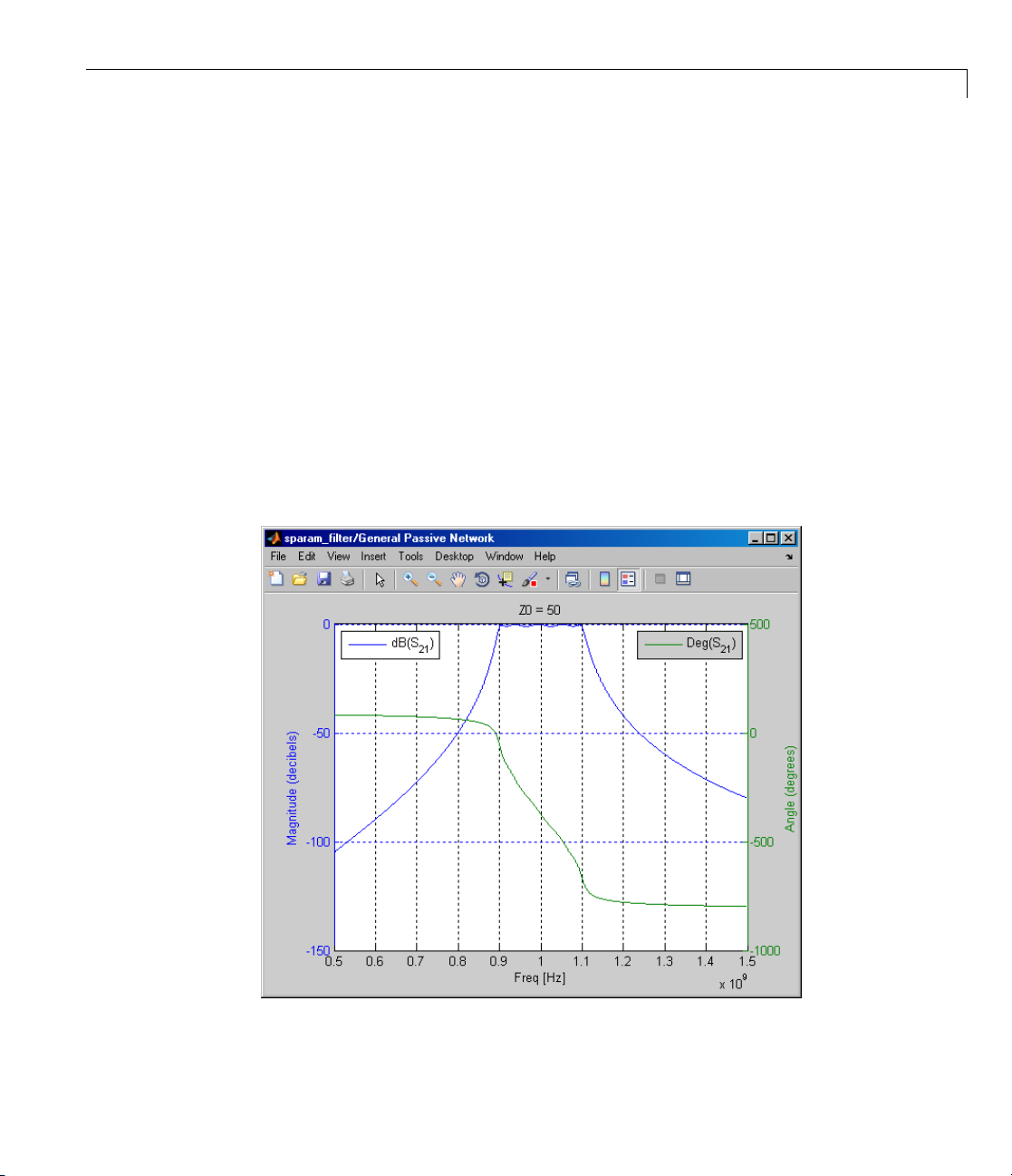
Validating the Passive Component

In this part of the example, you plot the network parameters of the General
Passive Network block to validate the data you imported in “Importing Data
into a General Passive Network Block” on page 2-10.

1 Open the General Passive Network block dialog box, and select the

Visualization tab.

2 Set the Source of frequency data parameter to User-specified.

3 Set the Frequencydata(Hz)parameter to [0.5e9:0.1e6:1.5e9].

4 Click Plot.

TheseactionscreateaplotofthemagnitudeandphaseofS
of frequency.

as a function

21

S21versus Frequency for the Imported Data

2-13

2 Modeling an RF System

Importing Circuits from the MATLAB Workspace

You can only connect the RF B locks et Physical blocks in cascade. However,
theblocksetworkswithRFToolboxsoftwaretoletyouincludeadditional
circuit topologies in an RF model. To model circuit topologies that contain
other types of connections, you must define a circuit in the MATLAB
workspace and import it into an RF model.

To import a circuit from the MATLAB works pace:

1 Define the circuit object in the MATLAB workspace using the RF Toolbox

functions.

For more information about RF circuit objects, see the RF Toolbox
documentation for “RF Circuit Objects”.

2 Add a General Circuit Element block to your RF model from the Black Box

Elements sublibrary of the Physical library. For information on how to
open this library, see “Openin g RF Blockset Libraries” on pa ge 1-6.

3 Enter the circuit object name in the RFCKT object parameter in the

General Circuit Element block dialog box.

2-14

This procedure is illustrated by example in the follow ing section.

Example — Importing a Bandstop Filter into an RF
Model

In this example, you simulate the frequency response of a filter that you
model using circuit objects from the MATLAB workspace.

The filter in this example is the 50-ohm bandstop filter shown in the following
figure.

Specifying or Importing Component Data

Bandstop F

You repres
four part
an input s
distribu

This exa

• “Creat

• “Build

• “Speci

• “Runn

ilter Diagram

ent the filter using four circuit objects that correspond to the

softhefilter,

ckt1, ckt2, ckt3,andckt4 in the diagram. You use

ignal with random, complex input values that have a Gaussian

tion to stimulate the filter. The scope block displays the output signal.

mple illustrates how to perform the following tasks:

ing Circuit Objects in the MATLAB Workspace” on page 2-15

ing the Model” on page 2-16

fying and Importing Component Data” on page 2-18

ing the Simulation and Plotting the Results” on page 2-19

Creating Circuit Objects in the MATLAB Workspace

is part of the example, you define MATLAB variables to represent the

In th

ical properties of the filter shown in the previous figure, Bandstop Filter

phys

ram on page 2-15, and use functions from RF Toolbox software to create

Diag

ircuit objects that model the filter components.

RF c

e the following at the MATLAB prompt todefinethefilter’scapacitance

1 Typ

inductance values in the MATLAB workspace:

and

2-15

2 Modeling an RF System

C1 = 1.734e-12;
C2 = 4.394e-12;
C3 = 7.079e-12;
C4 = 7.532e-12;
C5 = 1.734e-12;
C6 = 4.394e-12;
L1 = 25.70e-9;
L2 = 3.760e-9;
L3 = 17.97e-9;
L4 = 3.775e-9;
L5 = 17.63e-9;
L6 = 25.70e-9;

2 Type the follow ing at the MATLAB prompt to create RF circuit objects

that model the components labeled

ckt1, ckt2, ckt3,andckt4 in the

circuit diagram:

ckt1 = ...

rfckt.series('Ckts',{rfckt.shuntrlc('C',C1),...
rfckt.shuntrlc('L',L1,'C',C2)});

ckt2 = ...

rfckt.parallel('Ckts',{rfckt.seriesrlc('L',L2),...
rfckt.seriesrlc('L',L3,'C',C3)});

ckt3 = ...

rfckt.parallel('Ckts',{rfckt.seriesrlc('L',L4),...
rfckt.seriesrlc('L',L5,'C',C4)});

ckt4 = ...

rfckt.series('Ckts',{rfckt.shuntrlc('C',C5),...
rfckt.shuntrlc('L',L6,'C',C6)});

2-16

For more information about the RF Toolbox objects used in this example,
see the

rfckt.seriesrlc object reference pages in the RF Toolbox documentation.

rfckt.series class, rfckt.parallel, rfckt.shuntrlc,and

Building the Model

In this portion of the exam ple, you create a Simulink model. For more
information about adding and connecting components, see “Modeling RF
Components” on page 2-2.

1 Create a new model.

Specifying or Importing Component Data

2 Add to the model the blocks shown in the following table. The Library

column of the table specifies the hierarchical path to each block.

Block Library Quantity

Random Source Signal Processing

1

Blockset > Signal Processing
Sources

Input Port

RF Blockset > Physical

1

> Input/Output Ports

General Circuit
Element

Output Port

RF Blockset > Physical > Black
Box Elements

RF Blockset > Physical

4

1

> Input/Output Ports

Spectrum Scope Signal Processing

1

Blockset > Signal Processing
Sinks

3 Connect the blocks as shown in the following figure.

Change the names of your General Circuit Element blocks to match those
inthefigurebydouble-clickingthetextbelowtheblockandtypinganew
name.

2-17

2 Modeling an RF System

Specifying and Importing Component Data

In this portion of the example, you specify block parameters. To open the
parameter dialog b ox for each block, double-click the block.

1 In the Random Source block dialog box:

• Set the Source type parameter to

• Set the Sample time parameter to

• Set the Samples per frame parameter to

• Set the Complexity parameter to

Gaussian.

1/100e6.

256.

Complex.

Selecting these settings creates an input signal with random, complex
input values that have a Gaussian distribution.

2 In the Input Port block dialog box:

• Set the Treat input Simulink signal as parameter to

.

wave

• Set the Finite impulse response filter length parameter to

• Set the Center frequency (Hz) parameter to

• Set the Sample time parameter to

1/100e6.

400e6.

Incident power

256.

• Clear the Add noise check box.

Selecting these settings defines the physical characteristics and modeling
bandwidth of the filter.

3 Set the parameters of the General Circuit Element blocks as follows:

• In the General Circuit Element1 block dialog box, set the RFCKT

object parameter to

ckt1.

2-18

• In the General Circuit Element2 block dialog box, set the RFCKT

object parameter to

ckt2.

• In the General Circuit Element3 block dialog box, set the RFCKT

object parameter to

ckt3.

• In the General Circuit Element4 block dialog box, set the RFCKT

object parameter to

ckt4.

Specifying or Importing Component Data

Selecting these settings imports the circuit objects that model the filter
components into the model.

4 IntheOutputPortblockdialogbox,settheLoad impedance parameter

to

50.

5 Set the Spectrum Scope block parameters as follows:

• In the Scope Properties tab, set the Number of spectral averages

parameter to

100.

This parameter establishes the number of spectra that the scope
averages to produce the displayed signal. You use a value of 100 because
the input signal is random and you want to display the average filter
response over a large number of input values.

• In the Scope Properties tab, set the Spectrum units parameter to

dBm/Hertz.

• In the Axis Properties tab, set the Minimum Y-limit parameter to

-75 an d the Maximum Y-limit parameter to -45.

Thesevaluessettherangeofx-andy- va l ues on the display such that
the entire signal is visible when you run the simulation.

• In the Axis Properties tab, set the Y-axis label parameter to

dBm/Hertz.

Running the Simulation and Plotting the Results

In this part of the example, you run the simulation and examine the frequency
response of the filter.

Select Simulation > Start in the model window to start the simulation.

The Spectrum Scope window appears automatically and displays the following
plot, which shows the frequency response of the filter.

2-19

2 Modeling an RF System

2-20

Frequency Response of Bandstop Filter

The Spectrum Scope block displays the frequency response at the shifted
(baseband-equivalent) frequencies, not at the selected passband frequencies.
You can relabel the x-axis of the Spectrum Scope window to display the
passband signal by entering the Center frequency parameter value of

400e6 (fromtheInputPortblock)fortheFrequency display offset (Hz)

parameter in the Axis Properties tab of the Spectrum Scope block. For
more information on complex-baseband modeling, see “Cre ating a Complex
Baseband-Equivalent Model” on page A-13.

References

Geffe, P.R., “Novel designs for elliptic bandstop filters,” RF Design,February

1999.

Specifying Operating Conditions

Agilent P2D and S2D files contain simulation results at one or more operating
conditions. Operating conditions define the independent parameter settings
that are used when creating the file data. The specified conditions differ
from file to file.

Specifying Operating Conditions

When you import component data from a
AmplifierorGeneralMixerblock,theblock contains parameter values for
several operating conditions. The available conditions depend on the data in
the file. By default, the blockset defines the object behavior using the property
values that correspond to the operating conditions that appear first in the file.
To use other property values, you must select a different operating condition
in the block dialog box.

If the block contains data at multiple operating conditions, the Operating
Conditions tab contains two columns. The Conditions column shows the
available conditions, and the Values column contains a drop-down list of the
available values for the corresponding condition.

.p2d or .s2d file into a General

2-21

2 Modeling an RF System

Available
conditions

Lists of available
values for each
condition

Example Block Dialog Box Showing Operating Conditions

To specify the operating condition values for a simulation:

1 Double-click the block to open the block dialog box.

2 Select the Operating Conditions tab.

3 In the Conditions column, find the condition to specify. S el ect the

corresponding pull-down list in the Values column, and choose the desired
operating condition value.

Repeat the preceding step as needed to specify the desired operating condition
values.

2-22

Modeling Nonlinearity

In this section...

“Amplifier and Mixer Nonlinearity Specifications” on page 2-23

“Adding Nonlinearity to Your System” on page 2-24

Amplifier and Mixer Nonlinearity Specifications

You define nonlinearity for th e physical amplifier and mixer blocks at one or
more frequency points through one of the following specifi cations:

• Power data, consisting of output pow er as a function of input p ower,

imported into the block.

• Third-order intercept data, with or without power parameters, in the block

dialog box. The available power parameters are gain compression power
(defined as the ratio of output power to input power at small input power)
and output saturation power.

Modeling Nonlinearity

The following table summarizes the nonlinearity specification options for each
type of physical amplifier and mixer block.

Block

Genera

S-P

Y-P

Z-P

lAmplifier

arameters Amplifier

arameters Amplifier

arameters Amplifier

Nonline

You can
specif

• Power

• Third

Third-order intercept data or one or
more power parameters, in the block
dialog box.

arity Specification

choose either of the following

ications:

data (using a P2D, S2D, or

AMP da

or mo
bloc

ta file)

-order intercept data or one
re power parameters, in the

kdialogbox.

2-23

2 Modeling an RF System

Block

General Mixer You can choose either of the following

S-Parameters Mixer

Y-Parameters Mixer

Z-Parameters Mixer

Nonlinearity Specification

specifications:

• Power data (using a P2D, S2D, or

AMP data file)

• Third-order intercept data or one

or more power parameters, in the
block dialog box.

Third-order intercept data or one or
more power parameters, in the block
dialog box.

Adding Nonlinearity to Your System

To simulate the nonlinearity of an amplifier or mixer, you must specify or
import nonlinearity data at one or more frequency points into the block.

The method you use to add nonlinearity data to a block depends on whether
you specify the data manually or import the data into a block.

The following table provides instructions for adding nonlinearity data.

2-24

Nonlinearity Specification

IP3

Instructions

In the Nonlinearity Data tab of the block
dialog box:

• Set the IP3 type parameter to

OIP3.

• Enter input third-order intercept values

at one or more frequency points in the
IP3 (dBm) parameter.

• Enter corresponding frequency values in

the Frequency (Hz) parameter.

IIP3 or

Modeling Nonlinearity

Nonlinearity Specification

Power parameters

Instructions

Enter the gain compression power in the

1 dB gain compression power (dBm)

parameterorthesaturationpowerin
the Output saturation power (dBm)
parameter.

If you choose a scalar value for the
Frequency (Hz) parameter, then you
must also use scalar values for the power
parameters.

If you choose a vector value for the
Frequency (Hz) parameter, then you can
useeitherscalarorvectorvaluesforthe
power parameters.

Power data (from a file) Import file data that includes power

information into the Data file or RFCKT
object parameter of the General Amplifier
or General Mixer block.

Note If you import f ile data with no power information into a General
AmplifierorGeneralMixerblock,theNonlinearity Data tab lets you add
nonlinearity data manually in the block dialog box.

For information on how the blockset simulates nonlinearity data of an
amplifier or mixer, see the block reference page.

2-25

2 Modeling an RF System

Modeling Noise

In this section...

“Amplifier and Mixer Noise Specifications” on page 2-26

“Adding Noise to Your System” on page 2-27

“Plotting Noise” on page 2-31

Amplifier an d Mixer Noise Specifications

You only need to specify noise info rmation for the physical amplifier and mixer
blocks that generate noise other than resistor noise. For the other blocks, the
blockset calculates the noise automatically based on the resistor values.

You define nois e for the physical amplifier and mixer blocks through one of
the following specifications:

• Spot noise data in the data source.

2-26

• Spot noise data in the block dialog box.

• Spot noise data (

• Frequency-independent noise figure, noise factor, or noise temperature

value in the block dialog box.

• Frequency-dependent noise figure data (

dialog box.

Thefollowingtablesummarizesthenoise specification options for each type
of physical amplifier and mixer block.

rfdata.noise class) object in the block dialog box.

rfdata.nf) object in the block

Modeling Noise

Block

General Amplifier Spot noise data (using a Touchstone,

S-Parameters Amplifier

Y-Parameters Amplifier

Z-Parameters Amplifier

General Mixer Spot noise data (using a Touchstone,

S-Parameters Mixer

Y-Parameters Mixer

Z-Parameters Mixer

Noise Specification

P2D, S2D, or AMP data file)

OR

Spot noise data, noise figure value,
noise factor value, noise temperature
value,
object in the block dia lo g box

Spot noise data, noise figure value,
noise factor value, noise temperature
value,
object in the block dia lo g box

P2D, S2D, or AMP data file)

OR

Spot noise data, noise figure value,
noise factor value, noise temperature
value,
object in the block dia lo g box

Spot noise data, noise figure value,
noise factor value, noise temperature
value,
object in the block dia lo g box

rfdata.noise,orrfdata.nf

rfdata.noise,orrfdata.nf

rfdata.noise,orrfdata.nf

rfdata.noise,orrfdata.nf

Adding Noise to Your System

To simulate the noise of a physical subsystem, you perform the follo wing tasks:

• “Specifying or Importing Noise Data” on page 2-27

• “Adding Noise to the Simulation” on page 2-29

Specifying or Importing Noise Data

Themethodyouusetoaddnoisedatatoablockdependsonwhetheryouare
specifying noise data manually or importing spot-noise data.

2-27

2 Modeling an RF System

The following table provides instructions for adding noise data.

Noise Specification

Instructions

Frequency-independent noise figure In the Noise Data tab of the block

dialog box, set the Noise type
parameter to

Noise figure,and

enter the noise figure value in the
Noise figure (dB) parameter.

Frequency-dependent noise figure In the Noise Data tab of the block

dialog box, set the Noise type
parameter to
enter the name of the

Noise figure,and

rfdata.nf

object in the Noise figure (dB)
parameter.

Noise factor In the Noise Data ta b of the block

dialog box, set the Noise type
parameter to

Noise factor,and

enter the noise factor value in the
Noise factor parameter.

Noise temperature

In the Noise Data tab of the block
dialog box, set the Noise type
parameter to

Noise temperature,

and enter the noise temperature
value in the Noise temperature

(K) parameter.

2-28

Spot noise data (in a block dialog
box)

In the Noise Data tab of the block
dialog box, set the Noise type
parameter to

Spot noise data.

Enter the spot noise information in
the Minimum n oise figure (dB),
Optimal reflection coefficient,
and Equivalent normalized noise
resistance parameters.

Modeling Noise

Noise Specification

Instructions

Spot noise data (from a data object) In the Noise Data tab of the block

dialog box, set the Noise type
parameter to
enter the name of the

Noise figure and

rfdata.noise

object in the Noise figure (dB)
parameter.

Spot noise data (from a file) Import file data that includes noise

information into the Data file or
RFCKT object parameter of the
General A mplifier or General Mixer
block.

Note If you import file data with no noise information into a General
Amplifier or General Mixer block, the Noise Data tab lets you add noise
data manually in the block dialog box.

Adding Noise to the Simulation

To include noise in the simulation, you must select the Add noise check box
on the Input Port block dialog box. This check bo x is selected by default.

2-29

2 Modeling an RF System

2-30

Select this check box to
take the noise data in
the physical blocks into
account. This check box
is selected by default.

For information on how the blockset simulates noise, see “Modeling Noise in
an RF System” on page A-7.

Plotting Noise

RF Blockset soft
systems has a ver
contrast, the d
block is 1 Watt a
an RF system si
Blockset bloc

ware models communications systems. The noise in these

y small amplitude, typically from 1e-6 to 1e- 12 Watts. In

efault signal power of a Communications Blockset modulator

t a nominal 1 ohm. Therefore, the signal-to-noise ratio in

mulation is large, making it difficult to view the noise RF

ks add to your signal.

Modeling Noise

To display th
amplitude to

For example
test signal

source.

e noise on a plot, you might need to attenuate the signal
a value within a couple orders of magnitude of the noise.

, suppose you have the following model that contains a multitone

2-31

2 Modeling an RF System

When you simulate this model, Simulink brings up several windows showing
the input and output for the physical subsystem. The Input - Frequency
Domain window shown in the following figure displays the input signal in
the frequency domain.

2-32

Input Signal Spectrum

The Real Part of Input - Time Domain window displays the real part of the
complex-valued input signal i n the time domain.

Modeling Noise

Real Part of Input Signal

In the m odel, the physical subsystem adds noise to the input signal. The
Output - Frequency Domain window shows the noisy output signal in the
frequency domain.

Output Signal Spectrum

2-33

2 Modeling an RF System

The amplitude of the signal is large compared to the amplitude of the noise,
so the noise is not visible in the Real Part of Output - Time Domain w i ndow
that shows the real part of the time-domain output signal. Therefore, you
must attenuate the amplitude of the input signal to display the noise of the
time-domain output signal.

2-34

Real Par

Attenu
to

1e-3

you run
Output

tofOutputSignal

ate the amplitude of the input signal by setting the Gain parameter

. This is equivalent to attenuating the input signal by 60 dB. When

the m odel again, the two signal peaks are not as pronounced in the

- Frequency Domain window.

Modeling Noise

Output Signal Spectrum for Attenuated Input

You can now view the noise RF Blockset blocks add to your signal in the Real
Part of Output - Time Domain window.

Real Part of Output Signal Showing Noise

2-35

2 Modeling an RF System

2-36

Plotting Model Data

• “Creating Plots” on page 3-2

• “Updating Plots” on page 3-27

• “Modifying Plots” on page 3-28

• “Example — Creating and Modifying Subsystem Plots” on page 3-31

3

3 Plotting Model Data

Creating Plots

In this section...

“Available Data for Plotting” on page 3-2

“Using Plots to Validate Individual Blocks and Subsystems” on page 3-3

“Types of Plots” on page 3-3

“Plot Formats” on page 3-5

“How to Create a Plot” on page 3-14

“Example — Plotting Component Data on a Z Smith Chart” on page 3-22

Available Data for Plotting

RF Blockset software lets you validate the behavior of individual RF
components and physical subsystems in your model by plotting the following
data:

3-2

• Large- and small-signal S-parameters

• Noise figure, noise factor and noise temperature

• Output third-order intercept point

• Power data

• Phase noise

• Voltage standing-wave ratio

• Transfer function

• Group delay

• Reflection coefficients

Creating Plots

Note When you plot information about a physical block, the blockset plots
the actual frequency response of the block, as specified in the block dialog box.
The blockset does not plot the frequency response of the complex-baseband
model that it uses to simulate the block, in which the frequency response is
centered at zero. For more information on how the blockset simulates ph ysical
blocks, see Appendix A, “RF Block set Algorithms”.

Using Plots to Validate Individual Blocks and
Subsystems

You can plot model data for an individual physical block or for a physical
subsystem. A subsystem is a collection of one or more physical blocks
bracketed by an Input Port block and an Output Port block. To understand
thebehaviorofspecificsubsystems, plot the data of the corresponding Output
Port block after you run a simulation.

To validate the behavior of individual RF components in the model, plot the
data of the corresponding physical blocks. Y ou can plot data for individual
blocks from each of these co mponents either before or after you run a
simulation.

You create a plot by selecting options in the block dialog box, as shown in
“Example — Creating and Modifying Subsystem Plots” on page 3-31. To
learn about the available plots, see “Types of Plots” on page 3-3. For more
information about creating plots, see “How to Create a Plot” on page 3-14.

Types of Plots

RF Blockset software provides a variety of plots for analyzing the behavior
of RF components and subsystems. The following table summarizes the
available plots and charts and describes each one.

3-3

3 Plotting Model Data

Plot Type Plot Contents

X-Y Plane
(Rectangular) Plot

Link Budget Plot
(3-D)

Polar Plane Plot

Parameters as a function of frequency, input power,
or operating condition, such as

• S-parameters

• Noise figure (NF), Noise factor (NFactor), and

Noise Temperature (NTemp)

• Voltage standing-wave ratio (VSWR)

• Output third-order intercept point (OIP3)

• Input and output reflection coefficients

(GammaIn and GammaOut)

Parameters as a function of frequency for each
component in a physical subsystem

where

The curve for a given component represents the
cumulative contribution of e ach RF component
up to and including the parameter value of that
component.

For more information, see “Link Budget” on page
3-11.

Magnitude and phase of parameters as a function of
frequency or operating condition, such as

3-4

• S-parameters

• Input and output reflection coefficients

(GammaIn and GammaOut)

Smith Chart Real and imaginary parts of S-parameters as a

function of frequency or operating condition, used
for analyzing the reflections caused by impedance
mismatch.

Composite Plot Multiple plots and charts in one figure.

Tolearnhowtocreatetheseplots,see“HowtoCreateaPlot”onpage3-14.

Plot Formats

When you create a
the data for both

Creating Plots

plot from a block dialog box, you must specify the format of

the x-andy-axes.

These plot
the plot.

The availa
plot depe
the block
on the da
compute

The foll
plot ty

• “Compo

• “X-Y P

• “Link

• “Pol

options define how RF Blockset software displays the data on

ble formats vary with the data you select to plot. The data you can
nds on the plot type you select. The plot formats determine whether
set converts the data to a new set of units, or performs a calculation

ta. For example, setting the format to

and plot the real part of the parameter.

owing topics describe the available parameters and formats for each

pe:

site Data” on page 3-5

lane” on page 3-8

Budget” on page 3-11

ar Plane Plots and Smith Charts” on page 3-13

Real tells the blockset to

Composite Data

composite data plot automatically generates four separate plots in one

The

ure window, showing the frequency dependence of several parameters. The

fig

lowing figure shows an example of such a plot.

fol

3-5

3 Plotting Model Data

3-6

Example —

Note For

the form

The com
block d

or each specification. The Plot Contents column lists the types of plots

plot f
as the
upper

Composite Data Plot

composite data plots, you do not needtospecifytheparametersor

ats—they are set automatically.

bination of plots differs based on the type of block and the specified

ata. The following table describes the contents of the composite data

y appear on the composite plot, counterclockwise and starting in the

-left corner. The blockset plots all data as a function of frequency.

Creating Plots

Block

General
Amplifier
or General
Mixer

Other
Physical
block

Specified Da t a

Network parameters

OR

Network parameters and
noise

Network parameters and
power

OR

Network parameters, noise,
and power

Network parameters

OR

Network parameters
and noise (S-, Y-, and
Z-Parameters Amplifiers
and Mixers only)

Note Only the General
Amplifier and General
Mixer blocks accept power
data.

Plot Contents

• X-Y plot, magnitude of S

and S21in decibels

• X-Y plot, phase of S

12

and S

in degrees

• Z Smith Chart, real and

imaginary parts of S

11

and S

• Polar plot, magnitude and

phase of S

11

and S

22

• X-Y plot, magnitude of S

and S21in decibels

• X-Y plot, output power (P

in dBm (decibels referenced
to one milliwatt)

• Z Smith Chart, real and

imaginary parts of S

11

and S

• Polar plot, magnitude and

phase of S

11

and S

22

• X-Y plot, magnitude of S

and S21in decibels

• X-Y plot, phase of S

12

and S

in degrees

• Z Smith Chart, real and

imaginary parts of S

11

and S

• Polar plot, magnitude and

phase of S

11

and S

22

12

21

22

12

)

out

22

12

21

22

3-7

3 Plotting Model Data

X-Y Plane

You can plot any parameters that are relevant to your block on an X -Y plane
plot. For this type of plot, you specify data f or both the x-andy-axes. If you
specify two Y parameters, and you specify different formats for the two Y
parameters, the blockset plots the second Y parameter on the right y-axis.

The following table summarizes the available Y parameters and formats. The
parameters and formats are the same for both the left and right y-axes.

Note LS11, LS12, LS21,andLS22 are large-signal S-parameters. You can plot
these parameters as a function of input power or as a function of frequency.

Y Parameter Y Format

S11, S12, S21, S22

, LS12, LS21, LS22 (General

LS11

Amplifier and General Mixer blocks
with multiple operating conditions
only)

NF Magnitude (decibels)

NFactor None

NTemp Kelvin

OIP3 dBm

VSWRIn, VSWROut Magnitude (decibels)

Magnitude (decibels)
Magnitude (linear)
Angle (degrees)
Angle (radians)
Real
Imaginary

This format tells the blockset to plot
the noise factor as it is specified to or
calculated by the block.

dBW
W
mW

None

This format tells the blockset to plot
thevoltagestanding-waveratioas
it is specified to or calculated by the
block.

3-8

Y Parameter Y Format

Pout (General Amplifier and Ge neral

Mixer blocks with pow er data only)

Phase (General Amplifier and

General Mixer blocks with power

dBm
dBW
W
mW

Angle (degrees)
Angle (radians)

data only)

AM/AM (General A mplifier and

General Mixer blocks with power
data only)

Magnitude (decibels)
None

This format tells the blockset to
plot the AM/AM conversion as it
is specified to or calculated by the
block.

AM/PM (General A mplifier and

General Mixer blocks with power

Angle (degrees)
Angle (radians)

data only)

PhaseNoise (Mixer blocks only)

FMIN (Amplifier and Mixer blocks

with spot noise data only)

dBc/Hz

Magnitude (decibels)
None

This format tells the blockset to
plot the minimum noise figure as it
is specified to or calculated by the
block.

GammaIn, GammaOut(Output Port

block only)

Magnitude (decibels)
Magnitude (linear)
Angle (degrees)
Angle (radians)
Real
Imaginary

Creating Plots

3-9

3 Plotting Model Data

Y Parameter Y Format

GAMMAOPT (Amplifier a nd Mixer

blocks with spot no ise data only)

RN (Amplifier and Mixer blocks with

spot noise dat a only)

Magnitude (decibels)
Magnitude (linear)
Angle (degrees)
Angle (radians)
Real
Imaginary

None

This format tells the blockset to plot
the noise resistance as it is specified
to or calculated by the block.

The available X parameters depend on the Y parameters you select. The
following table summarizes the available X parameters for each of the Y
parameters in the preceding table.

Y Parameter X Parameter

Pout, Pha se, LS11, LS12, LS21, LS22 Pin

Freq

S11, S12 , S21, S22, NF, OIP3, VSWRIn,
VSWROut, GAMMAIn, GAMM AOu t, FMIN,
GAMMAOPT, RN

AM/AM, AM/PM AM

Freq

3-10

ThefollowingtableshowstheXformatsthatareavailablefortheX
parameters listed in the preceding table.

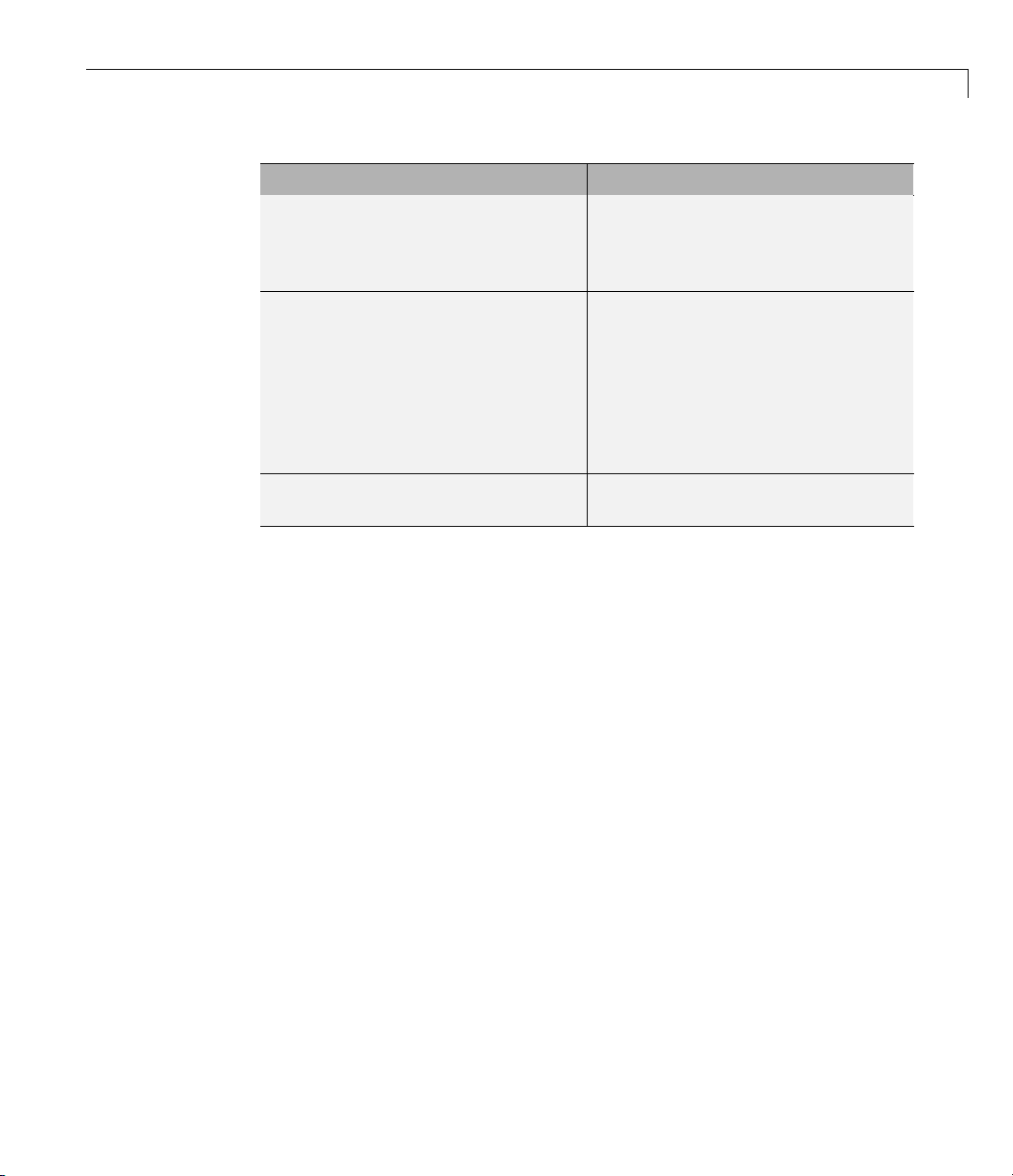
Creating Plots

XParameter XFormat

Pin dBm

dBW
W
mW

Freq THz

GHz
MHz
KHz
Hz

(xformat is chosen to provide

Auto

the best scaling for the given

xparameter values.)

AM Magnitude (dB)

Magnitude (linear)

When you import block data from a .p2d or .s2d file, you can also plot Y
parameters as a function of any operating condition from the file that has
numeric values, such as bias. You can specify an operating condition as the X
parameter only when validating individual blocks, and the format is always

None. This form at tells the blockset to plot the operating condition values as

they are specified in the file.

Link Budget

You use the Link budget plot to understand the individual contribution of
each block to a plotted Y parameter value in a physical subsystem with
multiple components between the Input Port and the Output Port blocks.

The link budget plot is a three-dimensionalplotthatshowsoneormorecurves
of parameter values as a function of frequency, ordered by the subsystem
circuit index.

The following figure shows how the circuit index is assigned to a component
in a physical subsystem based on its sequential position in the subsystem.

3-11

3 Plotting Model Data

Input Port

Component

(Index = 1)

Component
(Index = 2)

...

Component

(Index = n)

Output Port

A curve on the link budget plot for each circuit index represents the
contributions to the parameter value of the RF components up to that index.
The following figure shows an example of a link budget plot.

Contributions to S21
from components
1, 2, and 3

Contributions to S21
from components
1 and 2

Contributions to S21
from component 1

Example — Link Budget Plot

3-12

The following table summarizes the Y parameters and formats that are
available for a link budget plot.

Y Parameter Y Format

S11, S12, S21, S22 Magnitude (decibels)

Magnitude (linear)
Angle (degrees)
Real
Imaginary

OIP3 dBm

dBW
W
mW

Creating Plots

Y Parameter Y Format

NF Magnitude (decibels)

Magnitude (linear)

NFactor None

This format tells the blockset to plot
the noise factor as it is specified to
the block.

NTemp Kelvin

If you specify two Y parameters, the blockset puts both parameters in a single
plot. The Y parameters must have the same formats.

For a link budget plot, the X parameter is always

Freq.TheformatoftheX

parameter specifies the units of the x-axis.

Polar Plane Plots and Smith Charts

You can use R F Blockset software to generate Polar plots and Smith Charts.
When you select these plot types, you do not nee d to specify the format of
any Y parameters—the formats are set automatically. If you specify two Y
parameters, the blockset puts both parameters in a single plot.

The following table describes the Polar plot and Smith Chart options. It also
lists the available Y parameters.

Plot Type Y Parameter

Polar plane S11, S12, S21, S22

, LS12, LS21, LS22 (General

LS11

Amplifier and General Mixer blocks
with data from a P2D file only)

GammaIn, GammaOut (Output Port

block only)

Z Smith chart S11, S22

, LS22 (General Amplifier and

LS11

General Mixer blocks with data from
aP2Dfileonly)

3-13

3 Plotting Model Data

Plot Type Y Parameter

GammaIn, GammaOut (Output Port

block only)

Y Smith chart S11, S22

, LS22 (General Amplifier and

LS11

General Mixer blocks with data from
aP2Dfileonly)

GammaIn, GammaOut (Output Port

block only)

ZY Smith chart S11, S22

, LS22 (General Amplifier and

LS11

General Mixer blocks with data from
aP2Dfileonly)

GammaIn, GammaOut (Output Port

block only)

3-14

By default, the X parameter is Freq. The format of the X parameter specifies
the units of the x-axis. When you i mport block data from a

.p2d or .s2d file,

you can also plot Y parameters as a function of any operating condition from
the file that has numeric values, such as bias. You can specify an operating
condition as the X parameter only when validating individual blocks, and
the format is always

None.

How to Create a Plot

1 Double-click the block to open the block dialog box, and select the

Visualization tab. The following figure shows the contents of the tab.

2 Select the Source of frequency data.

Creating Plots

Select the source
of frequencies
at which to plot
block data

This value is the source of the frequency values at which to plot block
data. The following table summarizes the available types of sources for
the various types of blocks.

3-15

3 Plotting Model Data

Source of
frequency
data

User-specified

Description

Vector of freque ncies that you
enter.

When you select

User-specified in the Source

of frequency data list, the
Frequency range (Hz)

field is displayed. Enter a
vector specifying the range of
frequencies y ou want to plot.

For example, to plot block
data from 0.3 MHz to 5
GHz by 0.1 MHz, enter

[0.3e6:0.1e6:5e9].

Note When you select

PhaseNoise in the Parameter
list and

User-specified in the

Source of frequen cy data list,
the Frequency range (Hz)
field is disabled. You use the

Phase noise frequency offset
(Hz) block parameter to specify

the frequency values at which
to plot block data.

Blocks

Allphysicalblocks

3-16

Derived from
Input Port
parameters

(Available
after running
asimulation
or clicking
the Update

Modeling frequencies derived
from the Input Port block
parameters. For information
on how the blockset computes
the modeling frequencies, see
“Determining the Modeling
Frequencies” on page A-3.

Allphysicalblocks

Creating Plots

Source of
frequency
data

Diagram

button

Same as the
S-parameters

Same as the
Y-paramete

Same as the
Z-parameters

Extracted
from data
source

)

rs

Description

Frequency val
in the Frequen

ues specified

cy block

parameter.

Frequency v
in the Frequ
parameter

alues specified

ency block

.

Frequency values specified
in the Frequency block
parameter.

Frequency values imported
into the Data file or RFDATA
object block parameter.

Blocks

S-Parameters
Passive Netwo

rk,
S-Parameters
Amplifier,
S-Parameter

sMixer

Y-Parameters
Passive Network,
Y-Parameters
Amplifier,
Y-Parameters Mixer

Z-Parameters
Passive Network,
Z-Parameters
Amplifier,
Z-Parameters Mixer

General Passive
Network, General
Amplifier, and
General Mixer

3 Enter the Reference impedance.

3-17

3 Plotting Model Data

Enter the
reference
impedance

This value is the reference impedance to use w hen plotting small-signal
parameters.

4 Select the Plot type.

3-18

Select the
plot type

This value is the type of plot. For a description of the optio ns, see “Types
of Plots” on page 3-3.

5 Select the following parameters:

• Y Parameter1 — The first parameter for the Y-axis.

Creating Plots

• Y Parameter2 — The second parameter for the Y-axis (optional).

• X Parameter —TheparameterfortheX-axis.

Select the first Y-axis
plot parameter

Optionally, select
the second Y-axis
plot parameter

Select the X-axis
plot parameter

Theseparametersspecifythedatatobeplotted.Theavailablechoicesvary
with the type of plot. Fo r a description of the options for a particular plot
type, see the topic on that plot type in “Plot Formats” on page 3-5.

6 If you select a large-signal parameter for one or more y-axis parameters,

select the Source of power data.

Note Large-signal parameters are available only for General Amplifier or
General Mixer blocks that contain power data.

3-19

3 Plotting Model Data

Select the source
of input power
values at which
to plot block data

This value is the source of the input power values at which to plot block
data. The following table summarizes the available types of sources for the
General Amplifier and General Mixer blocks.

3-20

Source of frequency data

Extracted from data source

Description

Input power values imported into
the Data file or RFDATA object
block parameter.

User-specified

Vector of power values that you
enter.

When you select
in the Source of power data list,
the Input power data (dBm)
field is dis played. Enter a vector
specifying the range of power
values you want to plot.

For example, to plot block data
from 1 dBm to 10 dBm by 2 dBm,
enter

[1:2:10].

7 Select the following formats:

• YFormat1— The format for the first Y parameter.

User-specified

Creating Plots

• YFormat2— The format for the second Y parameter (optional).

• XFormat— The format for the X parameter.

Select the format
for Y parameter1

Optionally, select
the format for
Y parameter2

Select the format
for X parameter

ThesearetheXandYformatsforplotting the selected parameter. The
available choices vary based on the selected parameter. For a description
of the options for a particular plot type, see the topic on that plot type in
“Plot Formats” on page 3-5.

8 Select the XScaleand YScale.

3-21

3 Plotting Model Data

Select the
Y-axis scale

Select the
X-axis scale

These are the scales on which to plot the data. The available choices are

Linear and Log.

3-22

9 Click Plot.

Note By default, the blockset does not add a legend to some plots. To display

the plot legend, type

legend show at the MATLAB prompt.

Example — Plotting Component Data on a Z Smith
Chart

In this example, you simulate the frequency response of an amplifier using
data from the

Using a model from one of the RF Blockset demos, y ou import the data file
into a General Amplifier block and validate the amplifier by plotting the
S-parameters of the block on a Z Smith Chart.

1 Type sparam_amp attheMATLABprompttoopentheRFBlocksetdemo

called “AMP Data File for Amplifier”.

default.s2d S2D file.

Creating Plots

2 Double-click the G en eral Am plifier block to display its parameters.

3-23

3 Plotting Model Data

3-24

As shown in the preceding figure, the Data source parameter is set to

Data fileand the Data file parameter is set to default.s2d.These

values tell the blockset to import data from the file
uses this data, along with the other block parameters, in simulation.

3 Select the Visualization tab and set the General Amplifier block

parameters as follows:

• In the Plot type list, select

• In the Y Parameter1 list, select

Z Smith chart.

S22.

default.s2d.Theblock