Mathworks OPTIMIZATION TOOLBOX 5 user guide

Optimization Tool

User’s Guide

box™ 5

How to Contact The MathWorks

www.mathworks.
comp.soft-sys.matlab Newsgroup
www.mathworks.com/contact_TS.html T echnical Support

[e-mail] Product enhancement suggestions

bugs@mathwo
[e-mail] Documentation error reports
[e-mail] Order status, license renewals, passcodes

info@mathwo

com

rks.com

rks.com

Web

Bug reports

Sales, prici

ng, and general information

508-647-7000 (Phone)

508-647-7001 (Fax)

The MathWorks, Inc.
3 Apple Hill Drive
Natick, MA 01760-2098

For contact information about worldwide offices, see the MathWorks Web site.

Optimization Toolbox™ User’s Guide

© COPYRIGHT 1990–20 10 by The MathWorks, Inc.

The software described in this document is furnished under a license agreement. The software may be used
or copied only under the terms of the license agreement. No part of this manual may be photocopied or
reproduced in any form without prior written consent from The MathW orks, Inc.

FEDERAL ACQUISITION: This provision applies to all acquisitions of the Program and Documentation
by, for, or through the federal government of the United States. By accepting delivery of the Program
or Documentation, the government hereby agrees that this software or documentation qualifies as
commercial computer software or commercial computer software documentation as such terms are used
or defined in FAR 12.212, DFARS Part 227.72, and DFARS 252.227-7014. Accordingly, the terms and
conditions of this Agreement and only those rights specified in this Agreement, shall pertain to and govern
theuse,modification,reproduction,release,performance,display,anddisclosureoftheProgramand
Documentation by the federal government (or other entity acquiring for or through the federal government)
and shall supersede any conflicting contractual terms or conditions. If this License fails to meet the
government’s needs or is inconsistent in any respect with federal procurement law, the government agrees
to return the Program and Docu mentation, unused, to The MathWorks, Inc.

Trademarks

MATLAB and Simulink are registered trademarks of The MathWorks, Inc. See

www.mathworks.com/trademarks for a list of additional trademarks. Other product or brand

names may be trademarks or registered trademarks of their respective holders.

Patents

The MathWorks products are protected by one or more U.S. patents. Please see

www.mathworks.com/patents for more information.

Revision History

November 1990 First printing
December 1996 Second printing For MATLAB

®

5
January 1999 Third printing For Version 2 (Release 11)
September 2000 Fourth printing For Version 2.1 (Release 12)
June 2001 Online only Revised for Version 2.1.1 (Release 12.1)
September 2003 Online only Revised for Version 2.3 (Release 13SP1)
June 2004 Fifth printing Revised for Version 3.0 (Release 14)
October 2004 Online only Revised for Version 3.0.1 (Release 14SP1)
March 2005 Online only Revised for Version 3.0.2 (Release 14SP2)
September 2005 Online only Revised for Version 3.0.3 (Release 14SP3)
March 2006 Online only Revised for Version 3.0.4 (Release 2006a)
September 2006 Sixth printing Revised for Version 3.1 (Release 2006b)
March 2007 Seventh printing Revised for Version 3.1.1 (Release 2007a)
September 2007 Eighth printing Revised for Version 3.1.2 (Release 2007b)
March 2008 Online only Revised for Version 4.0 (Release 2008a)
October 2008 Online only Revised for Version 4.1 (Release 2008b)
March 2009 Online only Revised for Version 4.2 (Release 2009a)
September 2009 Online only Revised for Version 4.3 (Release 2009b)
March 2010 Online only Revised for Version 5.0 (Release 2010a)

Acknowledgments

The MathWorks™ would like to acknowledge the following contributors to
Optimization Toolbox™ algorithms.

Thomas F. Coleman researched and contributed algorithms for constrained
and unconstrained minimization, nonlinear least squares and curve fitting,
constrained linear least squares, quadratic programming, and nonlinear
equations.

Dr. Coleman is Dean of Faculty of Mathematics and Professor of
Combinatorics and Optimization at University of Waterlo o.

Dr. Coleman has published 4 books and over 70 technical papers in the
areas of continuous optimization and computational methods and tools for
large-scale problems.

Yin Zhang researched and contributed the large-scale linear programming
algorithm.

Acknowledgments

Dr. Zhang is Professor of Computational and Applied Mathematics on the
faculty of the Keck Center for Interdisciplinary Bioscience Training at Rice
University.

Dr. Zhang has published over 50 technical papers in the areas of interior-point
methods for linear programming and computational mathematical
programming.

Acknowledgments

Getting Started

1

Product Overview ................................. 1-2

Introduction
Optimization Functions
Optimization T ool GUI

...................................... 1-2

............................ 1-2

............................. 1-3

Contents

Example: Nonlinear Constrained Minimization

Problem Formulation: Rosenbrock’s Function
Defining the Problem in Toolbox Syntax
Running the Optimization
Interpreting the Result

.......................... 1-7

............................. 1-12

............... 1-5

...... 1-4

.......... 1-4

Setting Up an Optimization

2

Introduction to Optimization Toolbox Solvers ........ 2-2

Choosing a Solver

Optimization Decision Table
Problems Handled by Optimization Toolbox Functions

Writing Objective Functions

Writing Objective Functions
Jacobians of Vector and Matrix Objective Functions
Anonymous Function Objectives
Maximizing an Objective

................................. 2-4

........................ 2-4

........................ 2-10

......................... 2-10

..................... 2-15

........................... 2-16

... 2-7

..... 2-12

Writing Constraints

Types of Constraints
Iterations Can Violate Constraints
Bound Constraints

................................ 2-17

............................... 2-17

................................ 2-19

................... 2-18

vii

Linear Inequality Constraints ....................... 2-20

Linear Equality Constraints
Nonlinear Constraints
An Exam ple Using All Types of Constraints

......................... 2-20

............................. 2-21

............ 2-23

Passing Extra Parameters

Anonymous Functions
Nested Functions
Global Variables

Setting Options

Default Options
Changing the Default Settings
Tolerances and Stopping Criteria
Checking Validity of Gradients or Jacobians
Choosing the Algorithm

................................. 2-28

.................................. 2-28

.................................... 2-30

................................... 2-30

.......................... 2-25

.............................. 2-25

....................... 2-30

.................... 2-36

........... 2-37

............................ 2-45

Examining Results

3

Current Point and Function Value .................. 3-2

Exit Flags and Exit Messages

Exit Flags
Exit Messages
Enhanced Exit Messages
Exit Message Options

........................................ 3-3

.................................... 3-5

.............................. 3-8

....................... 3-3

........................... 3-5

viii Contents

Iterations and Function C ounts

First-Order Optimality Measure

Unconstrained Optimality
Constrained Optimality—Theory
Constrained Optimality in Solver Form

Displaying Iterative Output

Introduction
Most Common Output Headings

...................................... 3-14

.......................... 3-11

........................ 3-14

..................... 3-10

.................... 3-11

..................... 3-11

............... 3-13

..................... 3-14

Function-Specific Output Headings ................... 3-15

Output Structures

Lagrange Multiplier Structures

Hessian

fminunc Hessian
fmincon Hessian

Plot F unctions

Example: Using a Plot Function

Output Functions

Introduction
Example: Using Output Functions

........................................... 3-23

................................. 3-21

..................... 3-22

.................................. 3-23

.................................. 3-24

.................................... 3-26

..................... 3-26

.................................. 3-32

...................................... 3-32

................... 3-32

Steps to Take A fter Running a Solver

4

Overview of Next Steps ............................ 4-2

When the Solver Fails

Too Many Iterations or Function Evaluations
No Feasible Point
Problem Unbounded
fsolve Could Not Solve Equation
Solver T akes Too Long

When the Solver Might Have Succeeded

Final Point Equals Initial Point
Local Minimum Possible

When the Solver Succeeds

What Can Be Wrong If The Solver Succeeds?

1. Change the Initial Point

2. Check N earby Points

.............................. 4-3

................................. 4-8

............................... 4-9

..................... 4-10

............................. 4-10

...................... 4-14

............................ 4-14

.......................... 4-22

.......................... 4-23

............................ 4-24

.......... 4-3

............. 4-14

........... 4-22

ix

3. Check your Objective and Constraint Functions ...... 4-25

Local vs. Global Optima

............................ 4-26

Optimization Tool

5

Getting Started with the Optimization Tool .......... 5-2

Introduction
Opening the Optimization Tool
Steps for Using the Optimization Tool

...................................... 5-2

...................... 5-2

................. 5-5

Running a Problem in the Optimization Tool

Introduction
Pausing and Stopping the Algorithm
Viewing Results
Final Point
Starting a New Problem
Closing the Optimization Tool

Specifying Certain Options

Plot Functions
Output function
Display to Command Window

Getting Help in the Optimization Tool

Quick Reference
Additional Help

Importing and Exporting Your Work

Exporting to the MATLAB Workspace
Importing Your Work
Generating a File

Optimization Tool Examples

About Optimization Tool Examples
Optimization T ool with the fmincon Solver
Optimization T ool with the lsqlin Solver

...................................... 5-6

.................. 5-7

................................... 5-7

....................................... 5-11

............................ 5-11

....................... 5-12

......................... 5-13

.................................... 5-13

................................... 5-14

....................... 5-14

............... 5-16

.................................. 5-16

................................... 5-16

................ 5-17

................ 5-17

.............................. 5-19

................................. 5-19

........................ 5-21

................... 5-21

............. 5-21

............... 5-25

......... 5-6

x Contents

Optimization Algorithms and Examples

6

Optimization Th eory Overview ..................... 6-2

Unconstrained Nonlinear Optimization

Definition
Large Scale fminunc Algorithm
Medium Scale fminunc Algorithm
fminsearch Algorithm

Unconstrained Nonlinear Optimization Examples

Example: fminunc Unconstrained Minimization
Example: Nonlinear Minimization with Gradient and

Hessian

Example: Nonlinear Minimization with Gradient and

Hessian Sparsity Pattern

Constrained Nonlinear Optimization

Definition
fmincon Trust Region Reflective Algorithm
fmincon Active Set Algorithm
fmincon SQP Algorithm
fmincon Interior Point Algorithm
fminbnd Algorithm
fseminf Problem Formulation and Algorithm

Constrained Nonlinear Optimization Examples

Example: Nonlinear Inequality Constraints
Example: Bound Constraints
Example: Constraints With Gradients
Example: Constrained Minimization Using fmincon’s

Interior-Point Algorithm With Analytic Hessian
Example: Equality and Inequality Constraints
Example: Nonlinear Minimization with Bound Constraints

and Banded Preconditioner
Example: Nonlinear Minimization with E quality

Constraints
Example: Nonl inear Minimization with a Dense but

Structured Hessian and Equality Constraints

........................................ 6-3

...................... 6-3

.................... 6-6

.............................. 6-11

....................................... 6-16

......................... 6-17

........................................ 6-20

........................ 6-26

............................ 6-36

..................... 6-37

................................ 6-41

........................ 6-47

....................... 6-59

.................................... 6-63

.............. 6-3

........ 6-14

................ 6-20

............ 6-20

........... 6-41

............ 6-45

................ 6-48

......... 6-58

........ 6-65

.... 6-14

...... 6-45

...... 6-51

xi

Example: Using Symbolic Math Toolbox Functions to

Calculate Gradients and Hessians
Example: One-Dim e n sional Sem i-In f inite Constraints
Example: Two-Dimensional Semi-Infinite Constraint

.................. 6-69

... 6-84

.... 6-87

Linear Programming

Definition
Large Scale Linear Programming
Active-Set Medium-Scale linprog Algorithm
Medium-Scale linprogSimplexAlgorithm

Linear Programming Examples

Example: Linear Programming with Equalities and

Inequalities
Example: Linear Programming with Dense Columns in the

Equalities

Quadratic Programming

Definition
Large-Scale quadprog Algorithm
Medium-Scale quadprog Algorithm

Quadratic Programming Examples

Example: Quadratic Minimization with Bound

Constraints
Example: Quadratic Minimization with a Dense b ut

Structured Hessian

........................................ 6-91

..................................... 6-105

........................................ 6-108

............................... 6-91

.................... 6-91

............ 6-95

.............. 6-99

..................... 6-104

.................................... 6-104

........................... 6-108

..................... 6-108

................... 6-113

.................. 6-118

.................................... 6-118

.............................. 6-120

xii Contents

Binary Integer Programming

Definition
bintprog Algorithm

Binary Integer Programming Example

Example: Investments with Constraints

Least Squares (Model Fitting)

Definition
Large-Scale Least Squares
Levenberg-Marquardt Method
Gauss-Newton Method

........................................ 6-126

................................ 6-126

........................................ 6-134

............................. 6-140

....................... 6-126

...................... 6-134

.......................... 6-135

....................... 6-139

.............. 6-129

............... 6-129

Least Squares (Model Fitting) Examples ............. 6-144

Example: Using lsqnonlin With a Simulink Model
Example: Nonlinear Least-Squares with Full Jacobian

Sparsity Pattern

Example: Linear Least-Squares with Bound

Constraints

Example: Jacobian Multiply Function with Linear Least

Squares

Example: Nonlinear Curve Fitting with lsqcurvefit

....................................... 6-153

................................ 6-150

.................................... 6-151

....... 6-144

...... 6-157

Multiobjective Optimization

Definition
Algorithms

Multiobjective Optimization Examples

Example: Using fminimax with a Simu link Model
Example: Signal Processing Using fgoalattain

Equation Solving

Definition
Trust-Region Dogleg Method
Trust-Region Reflective fsolve Algorithm
Levenberg-Marquardt Method
Gauss-Newton Method
\ Algorithm
fzero Algorithm

Equation Solving Examples

Example: Nonlinear Equations with Analytic Jacobian
Example: Nonlinear Equations with Finite-Difference

Jacobian
Example: Nonlinear Equations with Jacobian
Example: Nonlinear Equations with Jacobian Sparsity

Pattern

........................................ 6-160

....................................... 6-161

.................................. 6-173

........................................ 6-173

...................................... 6-180

................................... 6-180

....................................... 6-184

........................................ 6-188

........................ 6-160

.............. 6-166

.......... 6-169

........................ 6-174

.............. 6-176

....................... 6-179

............................. 6-179

......................... 6-181

.......... 6-185

....... 6-166

... 6-181

Selected Bibliography

.............................. 6-192

xiii

Parallel Computing for Optimization

7

Parallel Computing in Optimization Toolbox

Functions

Parallel Optimization Functionality
Parallel Estimation of Gradients
Nested Parallel Functions

Using Parallel Computing with fmincon, fgoalattain,

and fminimax

Using Parallel Computing with Multicore Processors
Using Parallel Com puting with a Multiprocessor

Network

Testing Parallel Computations

....................................... 7-2

.................. 7-2

..................... 7-2

.......................... 7-3

................................... 7-5

....................................... 7-6

....................... 7-7

.... 7-5

Improving Performance with Parallel Computing

Factors That Affect Speed
Factors That Affect Results
Searching for Global Optima

.......................... 7-8

......................... 7-9

........................ 7-9

External Interface

8

ktrlink: An Interface to KNITRO Libraries ........... 8-2

What Is ktrlink?
Installation and Configuration
Example Using ktrlink
Setting Options
Sparse Matrix Considerations

.................................. 8-2

....................... 8-2

............................. 8-4

................................... 8-8

....................... 8-9

Argument and Options Reference

9

.... 7-8

xiv Contents

Function Arguments ............................... 9-2

Input Arguments .................................. 9-2

Output Arguments

................................ 9-5

10

Optimization Options

Options Structure
Output Function
Plot Functions

.................................... 9-27

.............................. 9-7

................................. 9-7

.................................. 9-18

Function Reference

Minimization ...................................... 10-2

Equation Solving

Least Squares (Curve Fitting)

GUI

Utilities

.............................................. 10-3

........................................... 10-4

.................................. 10-2

...................... 10-3

11

A

Functions — Alphabetical List

Examples

Constrained Nonlinear Examples ................... A-2

Least Squares Examples

............................ A-2

xv

Unconstrained Nonlinear Examples ................. A-3

Linear Programming Examples

Quadratic Programming Examples

Binary Integer Programming Examples

Multiobjective Examples

Equation Solving Examples

........................... A-3

..................... A-3

.................. A-3

......................... A-4

............. A-3

Index

xvi Contents

Getting Started

• “Product Overview” on page 1-2

• “Example: Nonline ar Constrained Minimization” on page 1-4

1

1 Getting Started

Product Overview

Introduction

Optimization Toolbox provides widely us ed a lg orithms for standard
and large-scale optimization. These algorithms solve constrained and
unconstrained continuous and discrete problems. The toolbox includes
functions for linear programming, quadratic programming, binary integer
programming, nonlinear optimization, nonlinear least squares, systems of
nonlinear equations, and multiobjective optimization. You can use them to
find optimal solutions, perform tradeoff analyses, balance multiple design
alternatives, and incorporate optimization methods into algorithms and
models.

In this section...

“Introduction” on page 1-2

“Optimization Functions” on page 1 -2

“Optimization Tool GUI” on page 1-3

1-2

Key features:

• Interactive tools for defining and solving optimization problems and

monitoring solution progress

• Solvers for nonlinear and multiobjective o ptimizatio n

• Solvers for nonlinear least squares, data fitting, and nonlinear equations

• Methods for solving quadratic and linear programming problems

• Methods for solving binary integer programming problems

• Parallel computing support in selected con strai ned n on li near solvers

Optimization Functions

Most toolbox functions are MATLAB®function files, made up of MATLAB
statements that implement specialized optimization algorithms. You can view
the code for these functions using the statement

type function_name

Product Overview

You can extend the capabilities of Optimization Toolbox software by writing
your own functions, or by using the software in combination with other
toolboxes, or with the MATLAB or Simulink

®

environments.

Optimization Tool GUI

Optimization Tool (optimtool) is a graphical user interface (GUI) for selecting
a toolbox function, specifying optimization options, and running optimizations.
It provides a convenie nt interface for all optimization routines, including those
from Gl obal Optimization Toolbox software, which is licensed separately.

Optimization Tool makes it easy to

• Define and modify problems quickly

• Use the correct syntax for optimization functions

• Import and export from the MATLAB workspace

• Generate code containing your configuration for a solver and options

• Change parameters of an optimization during the execution of certain

Global Optimization Toolbox functions

1-3

1 Getting Started

Example: Nonlinear Constrained Minimization

In this section...

“Problem Formulation: Rosenbrock’s Function” on page 1-4

“Defining the Problem in Toolbox Syntax” on page 1-5

“Running the Optimization” on page 1-7

“Interpreting the Result” on page 1-12

Problem Formulation: Rosenbrock’s Function

Consider the problem of minimizing Rosenbrock’s function

2

fx x x x() ( ),=−

over the unit disk, i.e., the disk of radius 1 centered at the origin. In other

words, find x that minimizes the function f(x)overtheset
problem is a minimization of a nonlinear function with a nonlinear constraint.

()

2

21

+−100 1

2

1

2

xx

122

1+≤

.This

1-4

Note Rosenbrock’s function is a standard test function in optimization. It
has a unique minimum value of 0 attained at the point (1,1). Finding the
minimum is a challenge for some algorithms since it has a shallow minimum
inside a deeply curved valley.

Here are two views of Ro senbrock’s function in the unit disk. The vertical
axis is log-scaled; in other words, the plot shows log(1 + f(x)). Contour lines
lie beneath the surface plot.

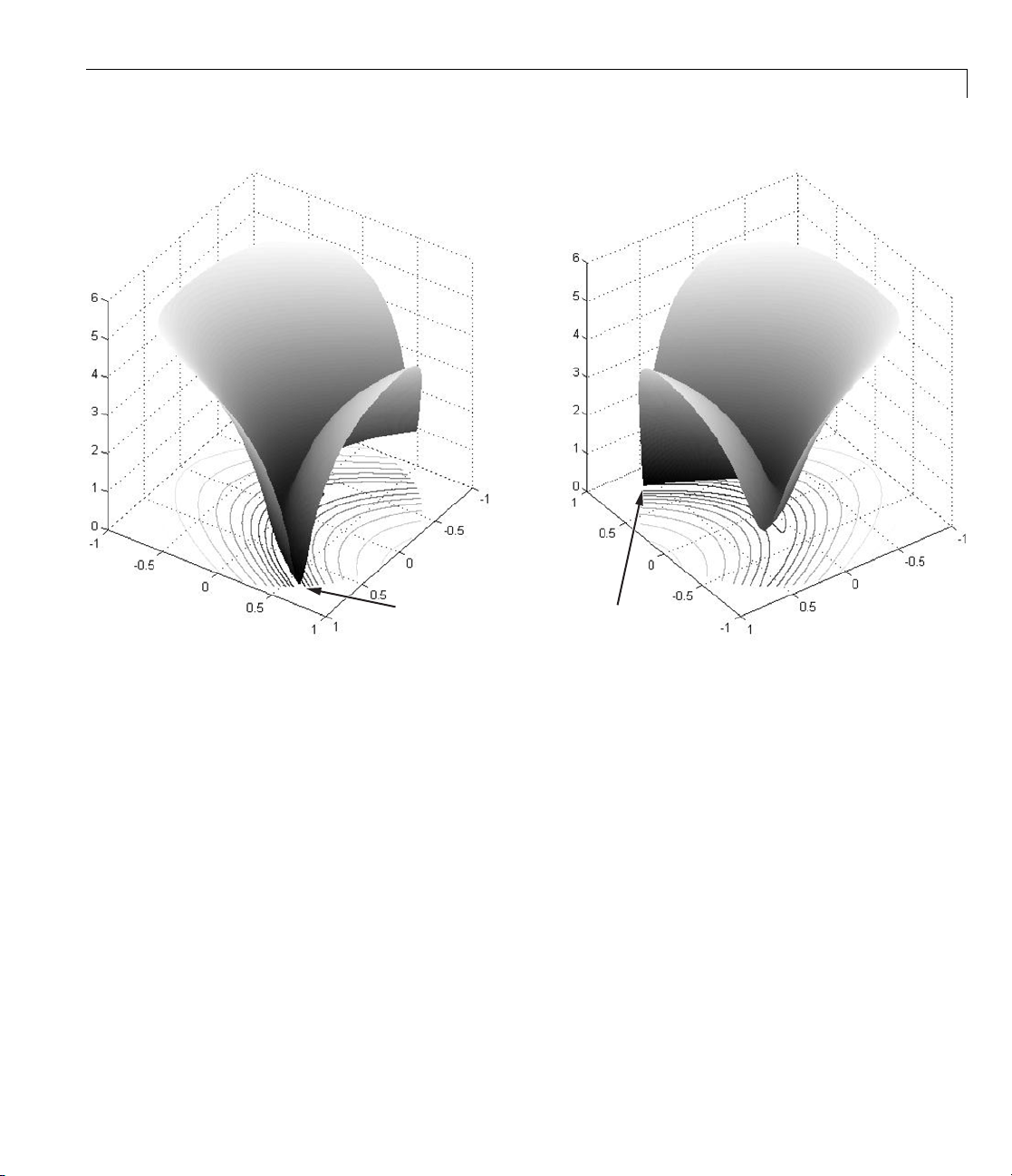
Example: Nonlinear Constrained Minimization

Minimum at (.7864, .6177)

Rosenbrock’s function, log-scaled: two views .

The function f(x)iscalledtheobjective function. This is the function you wish

to minimize. The inequality
limitthesetofx over which you may search for a minimum. You can have
any num ber of constraints, which are inequalities or equations.

All Optimization Toolbox optimization functions minimize an objective
function. To maximize a function f, apply an optimization routine to minimize
–f. For more details about maximizing, see “Maximizing an Objective” on
page 2-16.

Defining the Problem in Toolbox Syntax

To use Optimization Toolbox software, you need to

2

xx

122

is called a constraint. Constraints

1+≤

1-5

1 Getting Started

1 Define your objective function in the MATLAB language, as a function file

or anonymous function. This example will use a function file.

2 Define your constraint(s) as a separate file or anonymous function.

Function File for Objective Function

A function file is a text file containing MATLAB commands with the extension

.m. Create a new function file in any te xt editor, or use the buil t-in MATLAB

Editor as follows:

1 At the command line enter:

edit rosenbrock

The MATLAB Editor opens.

2 In the editor enter:

function f = rosenbrock(x)
f = 100*(x(2) - x(1)^2)^2 + (1 - x(1))^2;

1-6

3 SavethefilebyselectingFile > Save.

File for Constraint Function

Constraint functions must be formulated so that they are in the form

2

c(x) ≤ 0orceq(x)=0. Theconstraint

2

xx

122

10+−≤

in order to have the correct syntax.

xx

122

Furthermore, toolbox functions that accept nonlinear constraints need to
have both equality and inequality constraints defined. In this example there
is only an inequali ty constraint, so you must pass an empty array
the equality constraint function ceq.

With these considerations in mind, write a function file for the nonlinear
constraint:

1 Create a file named unitdisk.m containing the following code:

needs to be reformulated as

1+≤

[]as

Example: Nonlinear Constrained Minimization

function [c, ceq] = unitdisk(x)
c = x(1)^2 + x(2)^2 - 1;
ceq = [ ];

2 Save the file unitdisk.m.

Running the Optimization

Therearetwowaystoruntheoptimization:

• Using the “Optimization Tool” on page 1-7 Graphical User Interface (GUI)

• Using command line functions; see “Minimizing at the Command Line”

on page 1-11.

Optimization Tool

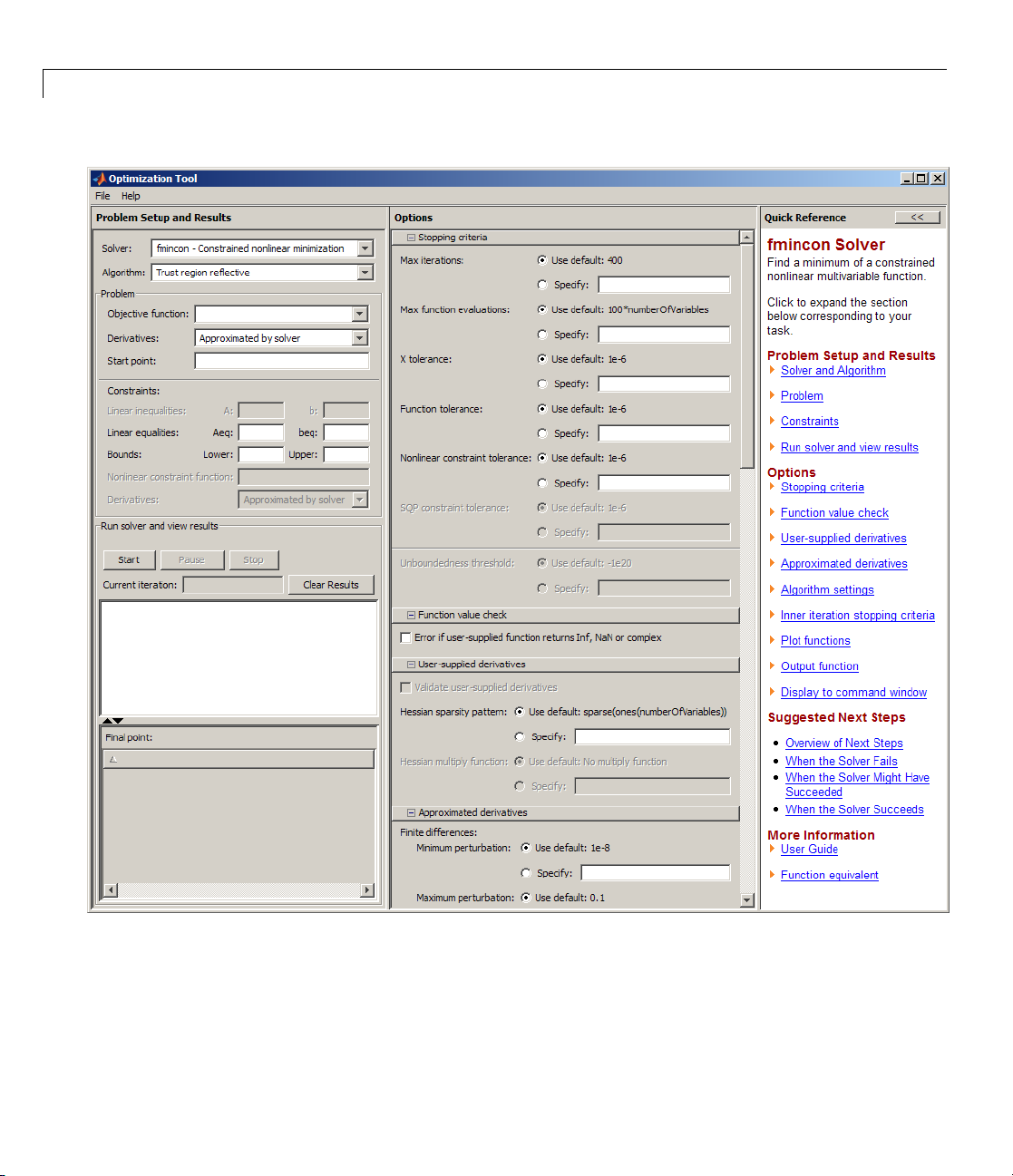
1 Start the Optimization Tool by typing optimtool at the command line.

The following GUI opens.

1-7

1 Getting Started

1-8

ore information about this tool, see Chapter 5, “Optimization Tool”.

For m

2 The default Solver fmincon - Constrained nonlinear minimization

isselected. Thissolverisappropriatefor this problem, since Rosenbrock’s

function is nonlinear, and the problem has a constraint. For more

Example: Nonlinear Constrained Minimization

information a bout how to choose a solver, see “Choosing a Solver” on page

2-4.

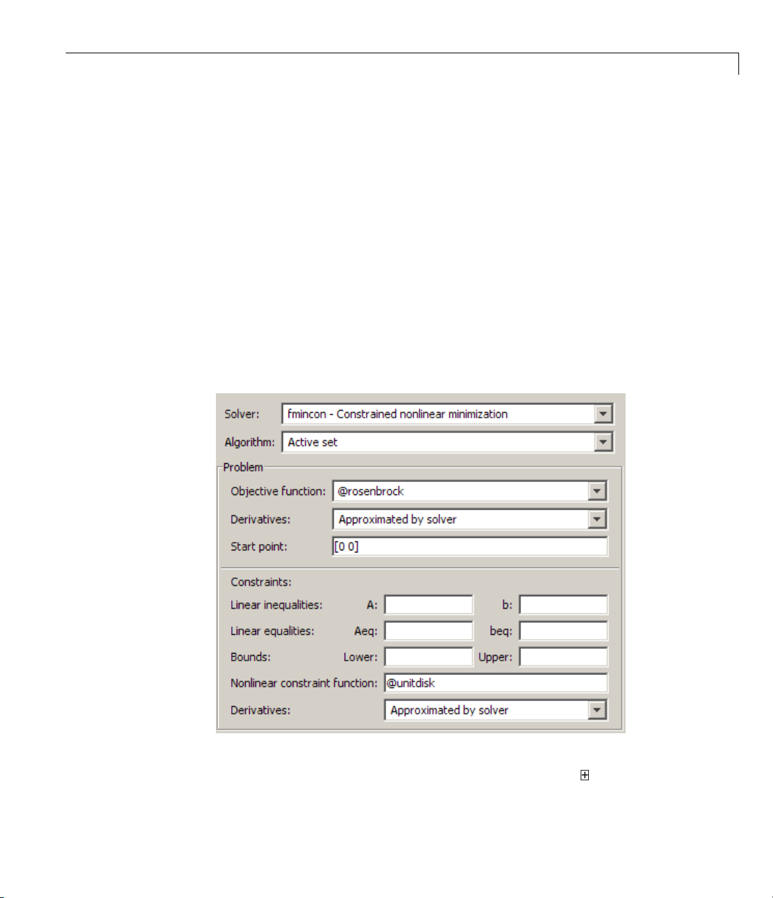
3 In the Algorithm pop-up menu choose Active set—the default Trust

region reflective

4 For Objective function enter @rosenbrock. The @ character indicates

that this is a function handle of the file

5 For Start point enter [0 0]. This is the initial point where fmincon

algorithm doesn’t handle nonlinear constraints.

rosenbrock.m.

begins its search for a minimum.

6 For Nonlinear constraint function enter @unitdisk, the function

handle of

unitdisk.m.

Your Problem Setup and Results pane should match this figure.

7 In the Options pane (center bottom), select iterative in the Level of

display pop-up menu. (If you don’t see the option, click

Display to

1-9

1 Getting Started

command window.) This shows the progress of fmincon in th e command

window.

8 Click Start un

der Run solver and view results.

The following message appears in the box below the Start button:

Optimization running.

Objective function value: 0.045674808692966654

Local minimum possible. Constraints satisfied.

fmincon stopped because the predicted change in the objective function

is less than the default value of the function tolerance and constraints

were satisfied to within the default value of the constraint tolerance.

Your objective function value may differ slightly, depending on your computer
system and version of O p timization Toolbox software.

The message tells y ou that:

• The search for a constrained optimum ended because the derivative of the

objective function is nearly 0 in directions allowed by the constraint.

1-10

• The constraint is very nearly satisfied.

“Exit Flags a n d Exit Messages” on p a ge 3-3 discusses exit messages such
as these.

The minimizer

x appears under Final point.

Example: Nonlinear Constrained Minimization

Minimizing at the Command Line

You can run the same optimization from the command line, as follows.

1 Create an options structure to choose iterative display and the active-set

algorithm:

options = optimset('Display','iter','Algorithm','active-set');

2 Run the fmincon solver with the options structure, reporting both the

location

function:

x of the minimizer, and value fval attained by the objective

[x,fval] = fmincon(@rosenbrock,[0 0],...

[],[],[],[],[],[],@unitdisk,options)

The six sets of empty brackets represent optional constraints that are not

being used in this example. See the

fmincon function reference pages for

the syntax.

MATLAB outputs a table of iterations, and the results of the optimization:

Local minimum possible. Constraints satisfied.

fmincon stopped because the predicted change in the objective function

is less than the default value of the function tolerance and constraints

were satisfied to within the default value of the constraint tolerance.

<stopping criteria details>

Active inequalities (to within options.TolCon = 1e-006):

lower upper ineqlin ineqnonlin

1

x=

0.7864 0.6177

1-11

1 Getting Started

fval =

0.0457

The message tells you that the search for a constrained optimum ended
because the derivative of the objective function is nearly 0 in directions
allowed by the constraint, and that the constraint is very nearly satisfied.
Several phrases in the message contain links that give you more information
about the terms used in the message. For more details about these links, see
“Enhanced Exit Mes sages” on page 3-5.

Interpreting the Result

The iteration table in the command window shows how MATLAB searched for
the minimum value of Rosenbrock’s function in the unit disk. This table is
the same whether you use Optimization Tool or the command line. MATLAB
reports the minim ization as follows:

Max Line search Directional First-order

Iter F-count f(x) constraint steplength derivative optimality Procedure

03 1 -1

1 9 0.953127 -0.9375 0.125 -2 12.5

2 16 0.808446 -0.8601 0.0625 -2.41 12.4

3 21 0.462347 -0.836 0.25 -12.5 5.15

4 24 0.340677 -0.7969 1 -4.07 0.811

5 27 0.300877 -0.7193 1 -0.912 3.72

6 30 0.261949 -0.6783 1 -1.07 3.02

7 33 0.164971 -0.4972 1 -0.908 2.29

8 36 0.110766 -0.3427 1 -0.833 2

9 40 0.0750939 -0.1592 0.5 -0.5 2.41

10 43 0.0580974 -0.007618 1 -0.284 3.19

11 47 0.048247 -0.003788 0.5 -2.96 1.41

12 51 0.0464333 -0.00189 0.5 -1.23 0.725

13 55 0.0459218 -0.0009443 0.5 -0.679 0.362

14 59 0.0457652 -0.0004719 0.5 -0.4 0.181

15 63 0.0457117 -0.0002359 0.5 -0.261 0.0905 Hessian modified

16 67 0.0456912 -0.0001179 0.5 -0.191 0.0453 Hessian modified

17 71 0.0456825 -5.897e-005 0.5 -0.156 0.0226 Hessian modified

18 75 0.0456785 -2.948e-005 0.5 -0.139 0.0113 Hessian modified

19 79 0.0456766 -1.474e-005 0.5 -0.13 0.00566 Hessian modified

1-12

Example: Nonlinear Constrained Minimization

This table might differ from yours depending on to olbo x ve rsio n and computing
platform. The following description applies to the table as displayed.

• The first column, labeled

fmincon took 19 iterations to converge.

• The second column, labeled

Iter, is the iteration number from 0 to 19.

F-count, reports the cumulative number

of times Rosenbrock’s function was evaluated. The final row shows an

F-count of 79, indicating that fmincon evaluated Rosenbrock’s function

79 times in the process of finding a minimum.

• The third column, labeled

f(x), displays the value of the objective function.

The final value, 0.0456766, is the minimum that is reported in the

Optimization Tool Run solver and view results box, and at the end of

the exit message in the com ma nd window.

• The fourth column,

Max constraint, goes from a value of –1 at the initial

value, to very nearly 0, –1.474e–005, at the final iteration. This column

shows the value of the constraint function

the value of

unitdisk was nearly 0 at the final iteration,

unitdisk at each iteration. Since

2

xx

122

1+≈

there.

The other columns of the iteration table are described in “Displaying Iterative
Output” on page 3-14.

1-13

1 Getting Started

1-14

2

Setting Up an Optimization

• “Introduction to Optimization Toolbox Solvers” on page 2-2

• “Choosing a Solver” on page 2-4

• “Writing Objective Functions” on page 2-10

• “Writing Constraints” on page 2-17

• “Passing Extra Parameters” on page 2-25

• “Setting Options” on page 2-30

2 Setting Up an Optimization

Introduction to Optimization Toolbox Solvers

There are four general categories of Optimization Toolbox solvers:

• Minimizers

This group of solvers attempts to find a local minimum of the objective

function near a starting point

optimization, linear programming, quadratic programming, and general

nonlinear programming.

• Multiobjectiv e minimizers

This group of solvers attempts to ei ther minimize the maximum value of

a set of functions (

functions is below some prespecified values (

• Equation solvers

This group of solvers attempts to find a solution to a scalar- or vector-valued

nonlinear equation f(x)=0nearastartingpoint

be considered a form of optimization because it is equivalent to finding

the minimum norm of f(x)near

fminimax), or to find a location where a collection of

x0. They address problems of unconstrained

x0.

fgoalattain).

x0. Equation-solving can

2-2

• Least-Squares (curve-fitting) solvers

This group of solvers attempts to minimize a sum of squares. This type of

problem frequently arises in fitting a model to data. The s olv ers address

problems of finding nonnegative solutions, bounded or linearly constrained

solutions, and fitting parameterized nonlinear models to data.

For more information see “Problems Handled by Optimization Toolbox
Functions” on page 2-7. See “Optimization Decis ion Table” on page 2-4 for
aid in choosing among solvers for minimization.

Minimizers formulate optimization problems in the form

min ( ),xfx

possibly subject to constraints. f(x)iscalledanobjective function. In general,
f(x) is a scalar function of type

double. However, multiobjective optimization, equation solving, and some

sum-of-squares minimizers, can have vector or matrix objective functions F(x)

double,andx isavectororscalaroftype

Introduction to Optimization Toolbox™ Solvers

of type double. To use Optimization Toolbox solvers for maximization instead
of minimization, see “Maximizing an Objective” on page 2-16.

Write the objective function for a solver in the form of a function file or
anonymous function handle. You can s upply a gradient
and you can supply a Hessian for several solvers. See “Writing Objective
Functions” on page 2-10. Constraints have a special form, as described in
“Writing Constraints” on page 2-17.

∇

f(x) for many solvers,

2-3

2 Setting Up an Optimization

Choosing a Solver

Optimization Decision Table

The following table is designed to help you choose a solver. It does not address
multiobjective optimization or equation so lv in g. There are more details on
all the solvers in “Problems Handled by Optimization Toolbox Functions”
on page 2-7.

Usethetableasfollows:

1 Identifyyourobjectivefunctionasoneoffivetypes:

In this section...

“Optimization D ecision Table” on page 2-4

“Problems Handled by Optimization Toolbox Functions” on page 2-7

• Linear

2-4

• Quadratic

• Sum-of-squares (Least squares)

• Smooth nonlinear

• Nonsmooth

2 Identify your constraints as one of five types:

• None (unconstrained)

• Bound

• Linear (including bound)

• General smooth

• Discrete (integer)

3 Use

In

thetabletoidentifyarelevantsolver.

this table:

Choosing a Solver

• Blank entries means there is no Optimization Toolbox solver specifically

designed for this type of problem.

• * means relevant solvers are found in Global Optimization Toolbox

functions (licensed separately from Optimization Toolbo x solvers).

•

fmincon applies to most smooth objective functions with smooth

constraints. It is not listed as a preferred solver for least squares or linear

or quadratic programming because the listed solvers are usually more

efficient.

• The table has suggested functions, but it is not meant to unduly restrict

your choices. For example,

fmincon isknowntobeeffectiveonsome

nonsmooth problems.

• The Global Optimization Toolbox

ga function can be programmed to

address discrete problems. It is not listed in the table because additional

programming is needed to solve discrete problems.

2-5

2 Setting Up an Optimization

Solvers by Objective and Constraint

Constraint
Type

None

Bound

Linear

General
smooth

Discrete

Linear

n/a (f =const,
or min =

linprog,

−∞

Theory,
Examples

linprog,

Theory,
Examples

fmincon,

Theory,
Examples

bintprog,

Theory,
Example

Quadratic

quadprog,

Theory,

)

Examples

quadprog,

Theory,
Examples

quadprog,

Theory,
Examples

fmincon,

Theory,
Examples

Objective Type

Least
Squares

\,
lsqcurvefit,
lsqnonlin,

Theory,
Examples

lsqcurvefit,
lsqlin,
lsqnonlin,
lsqnonneg,

Theory,
Examples

lsqlin,

Theory,
Examples

fmincon,

Theory,
Examples

Smooth
nonlinear

fminsearch,
fminunc,

Theory,
Examples

fminbnd,
fmincon,
fseminf,

Theory,
Examples

fmincon,
fseminf,

Theory,
Examples

fmincon,
fseminf,

Theory,
Examples

Nonsmooth

fminsearch,*

*

*

*

2-6

Note This table does not list multiobjective solvers nor equation solvers. See
“Problems Handled by Optimization Toolbox Functions” on page 2-7 for a
complete list of problems addressed by O p tim i z a tion Toolbox functions.

Note Some solvers have several algorithms. For help cho osing, see “Choosing
the Algorithm” on page 2- 4 5.

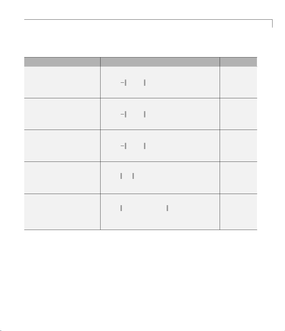
Problems Handled by Optimization Toolbox Functions

The following tables show the functions available for minimization, equation
solving, multiobjective optimization, and solving least-squares or data-fitting
problems.

Minimization Problems

Type Formulation Solver

Scalar minimization

min ( )xfx

such that l < x < u (x is scalar)

Unconstrained minimization

min ( )xfx

fminbnd

fminunc,
fminsearch

Choosing a Solver

Linear programming

Quadratic programming

Constrained minimization

T

min

fx

x

such that A·x ≤ b, Aeq·x = beq, l ≤ x ≤ u

1

min

TT

xHx cx

2

x

+

such that A·x ≤ b, Aeq·x = beq, l ≤ x ≤ u

min ( )xfx

such that c(x) ≤ 0, ceq(x)=0, A·x ≤ b,
Aeq·x = beq, l ≤ x ≤ u

linprog

quadprog

fmincon

2-7

2 Setting Up an Optimization

Minimization Problems (Continued)

Type Formulation Solver

Semi-infinite minimization

min ( )xfx

such that K(x,w) ≤ 0forallw, c(x) ≤ 0,
ceq(x)=0, A·x ≤ b, Aeq·x = beq, l ≤ x ≤ u

Binary integer programming

T

min

fx

x

such that A·x ≤ b, Aeq·x = beq, x binary

Multiobjective Problems

Type F ormul ation Solve r

Goal attainment

min

γ

,x γ

such that F(x)–w·γ ≤ goal, c(x) ≤ 0, ceq(x)=0,
A·x ≤ b, Aeq·x = beq, l ≤ x ≤ u

Minimax

min max ( )

x

such that c(x) ≤ 0, ceq(x)=0, A·x ≤ b,
Aeq·x = beq, l ≤ x ≤ u

i

Fx

i

fseminf

bintprog

fgoalattain

fminimax

Equation Solving Problems

Type F ormul ation Solve r

Linear equations

Nonlinear equation of one

C·x = d, n equations, n variables

f(x)=0

variable

Nonlinear equations

F(x)=0,n equations, n variables

2-8

\ (matrix left

division)

fzero

fsolve

Least-Squares (Model-Fitting) Problems

Type F ormul ation Solve r

Choosing a Solver

Linear least-squares

Nonnegative
linear-least-squares

Constrained
linear-least-squares

Nonlinear least-square s

Nonlinear curve fitting

1

minxCx d

2

⋅−

2
2

m equations, n variables

1

minxCx d

2

⋅−

2
2

such that x ≥ 0

1

minxCx d

2

⋅−

2
2

such that A·x ≤ b, Aeq·x = beq, lb ≤ x ≤ ub

min ( ) min ( )

xx

2

Fx F x

=

2

∑

2

i

i

such that lb ≤ x ≤ ub

min ( , )

Fxxdata ydata−

x

2
2

such that lb ≤ x ≤ ub

\ (matrix left

division)

lsqnonneg

lsqlin

lsqnonlin

lsqcurvefit

2-9

2 Setting Up an Optimization

Writing Objective Functions

In this section...

“Writing Objective Functions” on page 2-10

“Jacobians of Vector and Matrix Objective Functions” on page 2-12

“Anonymous Function Objectives” on page 2-15

“Maximizing an Objective” on page 2-16

Writing Objective Functions

This section relates to scalar-value d objective functions. A few solvers
require vector-valued objective functions:

lsqcurvefit,andlsqnonlin. For vector-valued or matrix-valued objective

functions, see “Jacobians o f Vector and Matrix Objective Functions” on page
2-12. For information on how to include extra parameters, see “Passing Extra
Parameters” on p age 2-25.

fgoalattain, fminimax, fsolve,

2-10

An objective function file can return one, two, or three outputs. It can return:

• A single double-precision number, representing the value of f(x)

• Both f(x)anditsgradient

∇

• All three of f(x),

You are not required to provide a gradient for some solvers, and you are
never required to provide a Hessian, but providing one or both can lead to
faster execution and more reliable answers. If you do not provide a gradient
or Hessian, solvers may attempt to estimate them using finite difference
approximations or other numerical schemes.

For constrained problems, providing a gradient has another advantage. A
solver can reach a point

x always lead to an infeasible point. In this case, a solver can fail or halt

prematurely. Providing a gradient allows a solver to proceed.

Some solvers do not use gradient or Hessian information. You shoul d
“conditionalize” a function so that it returns just what is needed:

f(x), and the Hessian matrix H(x)=∂2f/∂xi∂x

∇

f(x)

j

x such that x is feasible, but finite differences around

Writing Objective Functions

• f(x)alone

∇

• Both f(x)and

• All three of f(x),

Forexample,considerRosenbrock’sfunction

fx x x x() ( ),=−

which is described and plotted in “Example: Nonlinear Constrained
Minimization” on page 1-4. The gradient of f(x)is

f(x)

∇

f(x), and H(x)

2

2

()

21

+−100 1

2

1

⎡

−−

xxx x

400 2 1

()

∇fx

and the Hessian H(x)is

Hx

Function rosenboth returns the value of Rosenbrock’s function in f,the
gradient in

function [f g H] = rosenboth(x)
% Calculate objective f
f = 100*(x(2) - x(1)^2)^2 + (1-x(1))^2;

if nargout > 1 % gradient required

⎢
⎢

⎣

⎡

1200 400 2 400

() .=

⎢
⎢

⎣

g, and the Hessian in H if required:

g = [-400*(x(2)-x(1)^2)*x(1)-2*(1-x(1));

if nargout > 2 % Hessian required

end

⎢

() ,=

21211

200

2

xx x

−+−

1

−

400 200

200*(x(2)-x(1)^2)];

H = [1200*x(1)^2-400*x(2)+2, -400*x(1);

-400*x(1), 200];

−−

()

2

xx

−

()

21

21

x

1

⎤
⎥
⎥
⎥

⎦

⎤
⎥

⎥

⎦

end

2-11

2 Setting Up an Optimization

nargout checks the number of arguments that a calling function specifies; see

“Checking the Number of Input Arguments” in the MATLAB Programming
Fundamentals documentation.

The
to minimize Rosenbrock’s function. Tell
Hessian by setting

Run fminunc starting at [-1;2]:

fminunc solver, designed for unconstrained optimization, allows you

fminunc to use the gradient and

options:

options = optimset('GradObj','on','Hessian','on');

[x fval] = fminunc(@rosenboth,[-1;2],options)
Local minimum found.

Optimization completed because the size of the gradient
is less than the default value of the function tolerance.

x=

1.0000

1.0000

2-12

fval =

1.9310e-017

If you have a Symbolic Math Toolbox™ license, you can calculate gradients
and Hessians automatically, as described in “Example: Using Symbolic Math
Toolbox Functions to Calculate Gradients and Hessians” on page 6-69.

Jacobians of Vector and Matrix Objective Functions

Some solvers, s uch as fsolve and lsqcurvefit, have objective functions
that are vectors or matrices. T he only difference in usage between these
types of objective functions and scalar objective functions is the way to write
their derivatives. The first-order partial derivatives of a vector-valued or
matrix-valued function is called a Jacobian; the first-order partial derivatives
of a scalar function is called a gradient.

Writing Objective Functions

Jacobians of Vector Functions

If x represents a vector of independent variables, and F(x)isthevector
function, the Jacobian J(x) is defined as

Fx

()

∂

Jx

()

ij

If F has m components, and x has k components, J is a m-by-k matrix.

For example, if

i

.=

x

∂

j

Fx

()

⎡

xxx

+

1223

⎢
⎢

⎣

sin

23

xxx

+−

()

123

⎤

,=

⎥
⎥

⎦

then J(x)is

2

Jx

()

⎡

=

⎢

cos cos cos

⎣

xx x

13 2

23 2 23 3 23

xxx xxx xxx

+−

()

123 123 123

+−

()

−+−

(()

Jacobians of Matrix Functions

The Jacobian of a matrix F(x) is defined by changing the matrix to a vector,
column by column. For example, the matrix

FF

⎡

11 12

⎢

F

FF

=

21 22

⎢
⎢

FF

31 32

⎣

is rewritten as a vector f:

F

⎡

11

⎢

F

21

⎢
⎢

F

31

f

=

⎢

F

12

⎢
⎢

F

22

⎢

F

⎢

32

⎣

The Jacobian of F is defined as the Jacobian of f,

⎤
⎥
⎥
⎥

⎦

⎤
⎥
⎥
⎥

.

⎥
⎥
⎥
⎥

⎥

⎦

⎤

.

⎥
⎦

2-13

2 Setting Up an Optimization

If F is an m-by-n matrix, and x is a k-vector, the Jacobian is a mn-by-k matrix.

For example, if

the Jacobian of F is

J

ij

Fx

() / ,=

Jx

()

f

∂

i

=

.

x

∂

j

⎡

xx x x

12 132

⎢
⎢

xx xx

−

5

21421

⎢
⎢

⎣

⎡
⎢
⎢
⎢
⎢

=

⎢
⎢
⎢
⎢
⎢

⎣

2

xxx

−−

4

2

xx

21

3

x

−

45

1

02

2

xx

36

1

xx x

//

−

2121

2

xx

34

1

−

1

−

+

3

132

⎤⎤
⎥
⎥
⎥

x

2

⎥

.

⎥

2

⎥
⎥
⎥

3

⎥

2

⎦

2

⎤
⎥
⎥
⎥

4

⎥
⎦

2-14

Jacobians with Matrix-Valued Independent Variables

If x is a matrix, the Ja c ob ian of F(x) is defined by changing the matrix x to a
vector, column by column. For example, if

xx

⎡

11 12

X

=

⎢

xx

⎣

21 22

then the gradient is defined in terms of the vector

x

⎡

11

⎢

x

21

⎢

x

=

⎢

x

12

⎢

x

⎢

⎣

22

With

⎤

,

⎥
⎦

⎤
⎥
⎥

.

⎥
⎥

⎥

⎦

Writing Objective Functions

FF

⎡
⎢

F

=

⎢
⎢

⎣

11 12

FF

21 22

FF

31 32

⎤
⎥

,

⎥
⎥

⎦

and f the vector form of F as above, the Jacobian of F(X) is defined to be the
Jacobian of f(x):

f

∂

J

i

=

ij

.

x

∂

j

So, for example,

J

(,)

32

()

3

()

2

∂

31

=

X

∂

21

J

,(,)

and ..

54

f

()

∂

=

x

()

∂

f

∂

=

x

∂

F

∂

5
4

22

=

X

∂

22

F

If F is an m-by-n matrix, and x is a j-by-k matrix, the Jacobian is a mn-by-jk
matrix.

Anonymous Function Objectives

Anonymous functions are useful for writing simple objective functions.
For more information about anonymous functions, see “Constructing an
Anonymous Function”. Rosenbrock’s function is simple enough to write as an
anonymous function:

anonrosen = @(x)(100*(x(2) - x(1)^2)^2 + (1-x(1))^2);

Check that this evaluates correctly at (–1,2):

>> anonrosen([-1 2])
ans =

104

Using anonrosen in fminunc yields the following results:

options = optimset('LargeScale','off');
[x fval] = fminunc(anonrosen,[-1;2],options)

Local minimum found.

2-15

2 Setting Up an Optimization

Maximizing an Objective

All solvers are designed to minimize an objective function. If you have a
maximization problem, that is, a problem of the form

then define g(x)=–f(x), and minimize g.

For example, to find the maximum of tan(cos(x)) near x =5,evaluate:

Optimization completed because the size of the gradient
is less than the default value of the function tolerance.

x=

1.0000

1.0000

fval =

1.2262e-010

max ( ),

fx

x

2-16

[x fval] = fminunc(@(x)-tan(cos(x)),5)

Warning: Gradient must be provided for trust-region method;

using line-search method instead.

> In fminunc at 356

Local minimum found.

Optimization completed because the size of the gradient is less than

the default value of the function tolerance.

x=

6.2832

fval =

-1.5574

The maximum is 1.5574 (the negative of the reported fval), and occurs at
x = 6.2832. This is correct since, to 5 digits, the maximum is tan(1) = 1.5574,
which occurs at x =2π = 6.2832.

Writing Co nstraints

In this section...

“Types of Constraints” on page 2-17

“Iterations Can Violate Constraints” on page 2-18

“Bound Constraints” on page 2-19

“Linear Inequality Constraints” on page 2-20

“Linear Equality Constraints” on page 2-20

“Nonlinear Constraints” on p a ge 2-21

“An Example Using All Types of Constraints” on page 2-23

Types of Constraints

Optimization Toolbox solvers have special forms for constraints. Constraints
are separated into the following types:

Writing Constraints

• “Bound Constraints” on page 2-19 — Lower and upper bounds on individual

components: x ≥ l and x ≤ u.

• “Linear Inequality Constraints” on page 2-20 — A·x ≤ b. A is an m-by-n

matrix, w hich represents m constraints for an n-dimensional vector x. b is

m-dimensional.

• “Linear Equality Constraints” on page 2-20 — Aeq·x = beq. Thisisasystem

of equations.

• “Nonlinear Constraints” on page 2-21 — c(x) ≤ 0andceq (x)=0. Bothc and

ceq are scalars or vectors representing several constraints.

Optimization Toolbox functions assume that inequality constraints are of the
form c
constraints by multiplying them by –1. For example, a constraint of the form

c
A·x ≥ b is equivalent to the constraint –A·x ≤ –b. For more information, see

“Linear Inequality Constraints” on page 2-20 and “Nonlinear Constraints”
on page 2-21.

(x) ≤ 0orAx≤ b. Greater-than constraints are expressed as less-than

i

(x) ≥ 0 is equivalent to the constraint –ci(x) ≤ 0. A constraint of the form

i

2-17

2 Setting Up an Optimization

You can sometimes write constraints in a variety of ways. To make the best
use of the solvers, use the lowest numbered constraints possible:

1 Bounds

2 Linear equalities

3 Linear inequalities

4 Nonlinear equalities

5 Nonlinear inequalities

For example, with a constraint 5 x ≤ 20, use a bound x ≤ 4insteadofalinear
inequality or nonlinear inequality.

For information on how to pass extra parameters to constraint functions, see
“Passing Extra Parameters” on page 2-25.

2-18

Iterations Can Violate Constraints

Be careful when writing your objective and constraint functions. Intermediate
iterations can lead to points that are infeasible (do not satisfy constraints).
If you write objective or constraint functions that assume feasibility, these
functions can error or give unexpected results.

For example, if you take a square root or logarithm of x,andx <0,theresult
is not real. You can try to avoid this error by setting
Nevertheless, an intermediate iteration can violate this bound.

Algorithms that Satisfy Bound Constraints

Some solvers and algorithms honor bound constraints at every iteration.
These include:

•

fmincon interior-point, sqp,andtrust-region-reflective algorithms

lsqcurvefit trust-region-reflective algorithm

•

lsqnonlin trust-region-reflective algorithm

•

fminbnd

•

0 as a lower bound on x.

Writing Constraints

Algorithms that can Violate Bound Constraints

The following solvers and algorithms can violate bound constraints at
intermediate iterations:

•

fmincon active-set algorithm

fgoalattain

•

• fminimax

• fseminf

Bound Constraints

Lower and upper bounds on the components of the vector x. You need not give
gradients for this type of constraint; solvers calculate them automatically.
Bounds do not affect Hessians.

If you know bounds o n the location of your optimum, then you may obtain
faster and more reliable solutions by explicitly including these bounds in your
problem formulation.

Bounds are given as vectors, with the same length as x.

• If a particular component is not bounded below, use –

similarly, use

Inf if a component is not bounded above.

Inf as the bound;

• If you have only bounds of one type (upper or lower), you do not need

to write the other type. For example, if you have no upper bounds, you

do not need to supply a vector of

Infs. Also, if only the first m out of n

components are bounded, then you need only supply a vector of length

m containing bounds.

For example, suppose your bounds are:

• x

≥ 8

3

≤ 3

• x

2

Write the constraint vectors as

• l = [–Inf; –Inf; 8]

2-19

2 Setting Up an Optimization

• u =[Inf;3]oru = [Inf; 3; Inf]

Linear Inequality Constraints

Linear inequality constraints are of the form A·x ≤ b.WhenA is m-by-n,this
represents m constraints on a variable x with n components. You supply the
m-by-n matrix A and the m-component vector b. You do not need to give
gradients for this type of constraint; solvers calculate them automatically.
Linear inequalities do not affect Hessians.

For example, suppose that you have the following linear inequalities as
constraints:

Here m =3andn =4.

Write these using the following matrix A and vector b:

x

+ x3≤ 4,

1

2x

– x3≥ –2,

2

x

– x2+ x3– x4≥ 9.

1

2-20

1010

⎡
⎢

Ab=−

0210

⎢
⎢

−−

11 11

⎣

4

⎡

⎤

⎢

⎥

=

2

.

⎢

⎥

⎢

⎥

−

9

⎣

⎦

Notice that the “greater than” inequalities were first multiplied by –1 in order
to get them into “less than” inequality form.

⎤
⎥

,

⎥
⎥

⎦

Linear Equality Constraints

Linear equalities are of the form Aeq·x = beq.Thisrepresentsm equations
with n-component vector x. You supply the m-by-n matrix Aeq and the
m-component vector beq.Youdonotneedtogiveagradientforthistypeof
constraint; solvers calculate them automatically. Linear equalities do not
affect Hessians. The form of this type of constraint is exactly the same as
for “Linear Inequality Constraints” on page 2-20. Equalities rather than

Writing Constraints

inequalities are implied by the position in the input argument list of the
various solvers.

Nonlinear Constraints

Nonlinear inequality constraints are of the form c(x) ≤ 0, where c is a vector of
constraints, one component for each constraint. Similarly, nonlinear equality
constraints are of the form ceq( x)=0.

Nonlinear constraint functions must return both inequality and equality
constraints, even if they do not both exist. Return empty
constraint.

If you provide gradients for c and ceq, your solver may run faster and give
more reliable results.

[] fo r a n onexistent

Providing a gradient has another advantage. A solver can reach a point

x

such that x is feasible, but finite differences around x always lead to an
infeasible point. In this case, a solver can fail or halt prematurely. Providing
a gradient allow s a solver to proceed.

For e xample, suppose that you have the following inequalities as constraints:

2

xx

122

+≤

94

1

2

xx

≥−,.

21

1

Write these constraints in a function file as follows:

function [c,ceq]=ellipseparabola(x)
% Inside the ellipse bounded by (-3<x<3),(-2<y<2)
% Above the line y=x^2-1
c(1) = (x(1)^2)/9 + (x(2)^2)/4 - 1;
c(2) = x(1)^2 - x(2) - 1;
ceq = [];
end

ellipseparabola

returns empty [] as the nonlinear equality function. Also,

both inequalities were put into ≤ 0form.

2-21

2 Setting Up an Optimization

To include gradient information, write a conditionalized function as follows:

See “Writing Objective Functions” on page 2-10 for information on
conditionalized gradients. The gradient matrix is of the form

function [c,ceq,gradc,gradceq]=ellipseparabola(x)
% Inside the ellipse bounded by (-3<x<3),(-2<y<2)
% Above the line y=x^2-1
c(1) = x(1)^2/9 + x(2)^2/4 - 1;
c(2) = x(1)^2 - x(2) - 1;
ceq = [];

if nargout > 2

gradc = [2*x(1)/9, 2*x(1);...

x(2)/2, -1];

gradceq = [];

end

gradc

The first column of the gradient matrix is associated with
column is associated with

=[∂c(j)/∂xi].

i, j

c(1),andthesecond

c(2). This is the transpose of the form of Jacobians.

To have a solver use gradients of nonlinear constraints, indicate that they
exist by using

options=optimset('GradConstr','on');

optimset:

Make sure to pass the options structure to your solver:

[x,fval] = fmincon(@myobj,x0,A,b,Aeq,beq,lb,ub,...

@ellipseparabola,options)

If you have a license for Symbolic Math Toolbox software, you can calculate
gradients and Hessians automatically, as described in “Example: Using
Symbolic M ath Toolbox Functions to Calculate Gradients and Hessians” on
page 6-69.

2-22

Writing Constraints

An Example Using All Types of Constraints

This section contains an example of a nonlinear minimization problem with
all possible types of constraints. The objective function is in the subfunction

myobj(x). The nonlinear constraints are in the subfunction myconstr(x).

This example does not use gradients.

function fullexample
x0 = [1; 4; 5; 2; 5];
lb = [-Inf; -Inf; 0; -Inf; 1];
ub = [ Inf; Inf; 20];
Aeq = [1 -0.3 0 0 0];
beq = 0;
A = [0 0 0 -1 0.1

0 0 0 1 -0.5
0 0 -1 0 0.9];

b = [0; 0; 0];

[x,fval,exitflag]=fmincon(@myobj,x0,A,b,Aeq,beq,lb,ub,...

@myconstr)

%--------------------------------------------------------­function f = myobj(x)

f = 6*x(2)*x(5) + 7*x(1)*x(3) + 3*x(2)^2;

%--------------------------------------------------------­function [c, ceq] = myconstr(x)

c = [x(1) - 0.2*x(2)*x(5) - 71

0.9*x(3) - x(4)^2 - 67];

ceq = 3*x(2)^2*x(5) + 3*x(1)^2*x(3) - 20.875;

Calling fullexample produces the following display in the command window:

fullexample

Warning: Trust-region-reflective algorithm does not solve this type of problem, using active-set

algorithm. You could also try the interior-point or sqp algorithms: set the Algorithm option to

'interior-point' or 'sqp' and rerun. For more help, see Choosing the Algorithm in the documentation.

> In fmincon at 472

In fullexample at 12

2-23

2 Setting Up an Optimization

Local minimum found that satisfies the constraints.

Optimization completed because the objective function is non-decreasing in

feasible directions, to within the default value of the function tolerance,

and constraints were satisfied to within the default value of the constraint tolerance.

Active inequalities (to within options.TolCon = 1e-006):

lower upper ineqlin ineqnonlin

3

x=

0.6114

2.0380

1.3948

0.3587

1.5498

fval =

37.3806

2-24

exitflag =

1

Passing Extra Parameters

Sometimes objective or constraint functions hav e parameters in addition
to the independent variable. There are three methods of including these
parameters:

• “Anonymous Functions” on page 2-25

• “Nested Functions” on page 2-28

• “Global Variables” on page 2-28

Global variables are troublesome because they do not allow names to be
reused among functions. It is better to use one of the other two methods.

For example, suppose you want to minimize the function

fx a bx x x xx c cx x() ,

=− +

()

121

4312

/

++−+

12 222

Passing Extra Parameters

()

2

(2-1)

for diffe
depend o
how to pr
paramet

Anonym

To pass

1 Write

2 Ass

rent values of a, b,andc. Solvers accept objective functions that

nly on a single variable (x in th is case). The following sections show

ovide the additional parameters a, b,andc.Thesolutionsarefor

er values a =4,b =2.1,andc =4nearx

=[0.50.5]usingfminunc.

0

ous Functions

parameters using anonymous functions:

a file contain ing the follo wing code:

function y = parameterfun(x,a,b,c)
y = (a - b*x(1)^2 + x(1)^4/3)*x(1)^2 + x(1)*x(2) + ...

(-c + c*x(2)^2)*x(2)^2;

ign values to the parameters and define a function handle
nymous function by entering the following commands at the MATLAB

ano

mpt:

pro

a = 4; b = 2.1; c = 4; % Assign parameter values
x0 = [0.5,0.5];

f to an

2-25

2 Setting Up an Optimization

3 Call the solver fminunc with the anonymous function:

f = @(x)parameterfun(x,a,b,c)

[x,fval] = fminunc(f,x0)

The following output is displayed in the command window:

Warning: Gradient must be provided for trust-region algorithm;

using line-search algorithm instead.

> In fminunc at 347

Local minimum found.

Optimization completed because the size of the gradient is less than

the default value of the function tolerance.

x=

-0.0898 0.7127

2-26

fval =

-1.0316

Passing Extra Parameters

Note The parameters passed in the anonymous function are those that exist
at the time the anonymous function is created. Consider the example

a=4;b=2.1;c=4;
f = @(x)parameterfun(x,a,b,c)

Suppose you subsequently change, a to 3 and run

[x,fval] = fminunc(f,x0)

You get the same answer as before, since parameterfun uses a=4,thevalue
when

parameterfun was created.

To change the parameters that are passed to the function, renew the
anonymous function by reentering it:

a=3;
f = @(x)parameterfun(x,a,b,c)

You can create anonymous functions of more than one argument. For
example, to use
arguments,

fh = @(x,xdata)(sin(x).*xdata +(x.^2).*cos(xdata));
x = pi; xdata = pi*[4;2;3];
fh(x, xdata)

ans =

9.8696

9.8696

-9.8696

lsqcurvefit, first create a function that takes two input

x and xdata:

Now call lsqcurvefit:

% Assume ydata exists
x = lsqcurvefit(fh,x,xdata,ydata)

2-27

2 Setting Up an Optimization

Nested Function

To pass the param
file that

• Accepts

• Contains the o

• Calls

Here is the co

function [x,fval] = runnested(a,b,c,x0)
[x,fval] = fminunc(@nestedfun,x0);
% Nested function that computes the objective function

end

The obje
to the va

To run th

a, b, c,

fminunc

de for the function file for this example:

function y = nestedfun(x)

y = (a - b*x(1)^2 + x(1)^4/3)*x(1)^2 + x(1)*x(2) +...

end

ctivefunctionisthenestedfunction

riables

e optimization, enter:

a, b,andc.

s

eters for Equation 2-1 via a nested function, write a single

and

x0 as inputs

bjective function as a nested function

(-c + c*x(2)^2)*x(2)^2;

nestedfun, which has access

2-28

a = 4; b = 2.1; c = 4;% Assign parameter values
x0 = [0.5,0.5];
[x,fval] = runnested(a,b,c,x0)

The ou

Glob

Glob
glob
the

tput is the same as in “Anonymous Functions” on page 2-25.

al Variables

al va riab le s can be troublesome, it is better to avoid u sin g them. To u se

al variables, declare the variables to be global in the workspace and in

functions that use the variables.

te a function file:

1 Wri

function y = globalfun(x)

Passing Extra Parameters

global a b c
y = (a - b*x(1)^2 + x(1)^4/3)*x(1)^2 + x(1)*x(2) + ...

(-c + c*x(2)^2)*x(2)^2;

2 In your MATLAB workspace, define the variables and run fminunc:

global a b c;
a = 4; b = 2.1; c = 4; % Assign parameter values
x0 = [0.5,0.5];
[x,fval] = fminunc(@globalfun,x0)

The output is the same as in “Anonymous Functions” on page 2-25.

2-29

2 Setting Up an Optimization

Setting Options

Default Options

The options structure contains options used in the optimization routines.
If, on the first call to an optimization routine, the
provided, or is empty, a set of default options is generated. Some of the default
options values are calculated using factors based on problem size, such as

MaxFunEvals. Some options are dependent on the specific solver algorithms,

and a re documented on those solver f unction reference pages.

In this section...

“Default Options” on page 2-30

“Changing the Default Settings” on page 2-30

“Tolerances and Stopping Criteria” on page 2-36

“Checking Validity of Gradients or Jacobians” on page 2-37

“Choosing the Algorithm” on page 2-45

options structure is not

2-30

“Optimization Options” on page 9-7 provides an overview of all the options in
the

options structure.

Changing the Default Settings

The optimset function creates or updates an options structure to pass
to the various optimiz ation functions. The arguments to the
function are option name and option value pairs, such as TolX and 1e-4.Any
unspecified properties have default values. You need to type only enough
leading characters to define the option name uniquely. Case is ignored for
option names. For option values that are strings, however, case and the exact
string are necessary.

help optimset provides information that defines the different options and

describes how to use them.

Herearesomeexamplesoftheuseof

optimset.

optimset

Setting Options

Returning All Options

optimset returns all the options that can be set with typical values and

default values.

Determining Options Used by a Function

The options structure defines the options passed to solvers. Because
functions do not use all the options, it can be useful to find which options
are used by a particular function. There are several ways of determining
the available options:

• Consult the combined “Optimization Options” on page 9-7 table.

• To find detailed descriptions of the options and their default values,

consult the Options table in the function reference pages. For example, the

available options for

• To find available options at the command line, pass the name of the

function (in this example,

optimset('fmincon')

fmincon appear in this table.

fmincon)tooptimset:

or

optimset fmincon

or

optimset(@fmincon)

This statement returns a structure. Generally, fields not used by the

function have empty values (

[]); fields used by the function are set to their

default values for the given function. However, some solvers have different

default values depending on the algorithm used. For example,

adefault

active-set algorithms, but a default value of 1000 for the interior-point

MaxIter value of 400 for the trust-region-reflective, sqp,and

fmincon has

algorithm. optimset fmincon returns [] for the MaxIter field.

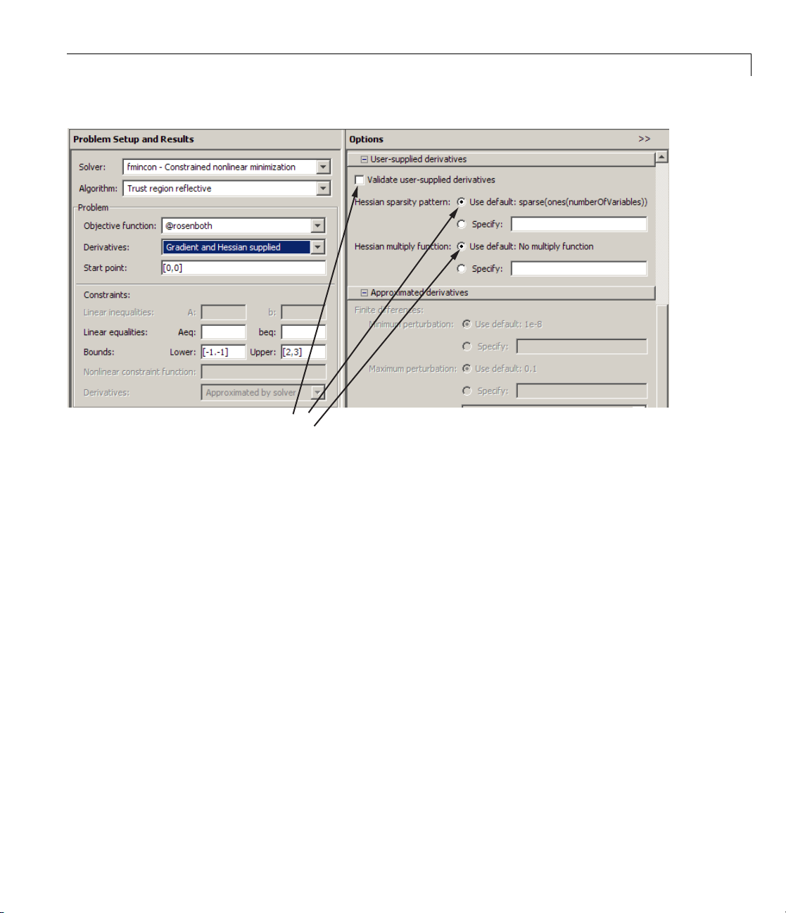
• You can also check the available options and their defaults in the

Optimization Tool. These can change depending on problem and algorithm

settings. These three pictures show how the available options for

derivatives change as the type of supplied derivatives change:

2-31

2 Setting Up an Optimization

Settable
options

2-32

Settable
options

Settable
options

Setting Options

Setting More Than One Option

You can specify multiple options with one call to optimset. For example, to
reset the

options = optimset('Display','iter','TolX',1e-6);

Display option and the tolerance on x,enter

Updating an options Structure

To update an existing options structure, call optimset and pass the existing
structure name as the first argument:

options = optimset(options,'Display','iter','TolX',1e-6);

Retrieving Option Values

Use the optimget function to get option values from an options structure.
Forexample,togetthecurrentdisplay option, enter the following:

verbosity = optimget(options,'Display');

2-33

2 Setting Up an Optimization

Displaying Output

To display output at each iteration, enter

This command sets the value of the Display option to 'iter', which causes
the solver to display output at each iter ation. You can also turn off any output
display (
output only if the problem fails to converge (

Choosing an Algorithm

Some solvers explicitly use an option called LargeScale for choosing which
algorithm to use:
the
instead: fmincon, fsolve, and others. All algorithms in Algorithm solvers
are large scale, unless otherwise noted in their function reference pages. The
term large-scale is explained in “Large-Scal e vs. Medium-Scale Algorithms”
on page 2-35. For all solvers that have a large-scale algorithm, the default
is for the function to use a large-scale algorithm (e.g.,

'on' by default).

options = optimset('Display','iter');

'off'), display output only at termination ('final'), or display

'notify').

fminunc, linprog, and others. O ther solvers do not use

LargeScale attribute explicitly, but have an option called Algorithm

LargeScale is set to

2-34

For help deciding which algorithm to use, see “Choosing the Algorithm” on
page 2-45.

To use a medium-scale algorithm in a solver that takes the

LargeScale

option, enter

options = optimset('LargeScale','off');

For solvers that use the Algorithm option, choose the algorithm by entering

options = optimset('Algorithm','algorithm-name');

algorithm-name

is the name of the chosen algorithm. You can find the

choices in the function reference pages for each solver.

Setting Options

Large-Scale vs. Medium-Scale Algorithms. An optimization algorithm
is large scale when it uses linear algebra that does not need to store, nor
operate on, full matrices. This may be done internally by storing sparse
matrices, and by using sparse linear algebra for computations whenever
possible. Fu r th erm ore, the internal algorithms either preserve sparsity, such
as a sparse Cholesky decomposition, or do not generate matrices, such as a
conjugate gradient method. Large-scale algorithms are accessed by setting
the

LargeScale option to on, or setting the Algorithm option appropriately

(this is solver-dependent).

In contrast, medium-scale methods internally create full matrices and use
dense linear algebra. If a problem is sufficiently large, full matrices take up a
significant amount of memory, and the dense linear algebra may require a
long time to execute. Medium-scale algorithms are accessed by setting the

LargeScale option to off, or setting the Algorithm option appropriately (this

is solver-dependent).

Don’t let the name “large-scale” mislead you; you can use a large-scale
algorithm on a small problem. Furthermore, you do not need to specify any
sparse matrices to use a la rge-scale algorithm. Choose a medium-scale
algorithm to access extra functionality, such as additional constraint types,
or possibly for better performance.

Defining Output Functions and Plot Functions

Output functions and plot functions give information on the progress of a
solver. They report results after each iteration of a solver. Additionally,
they can halt a solver. For more information and examples of their use, see
“Output Functions” on page 3-32 and “Plot Functions” on page 3-26.

Call output or plot functions by passing a function handle, or a cell array of
function handles. For output functions, the syntax is

options = optimset('OutputFcn',@outfun);

or

options = optimset('OutputFcn',...

outfun1,@outfun2,...});

{@

For plot functions, the syntax is

2-35

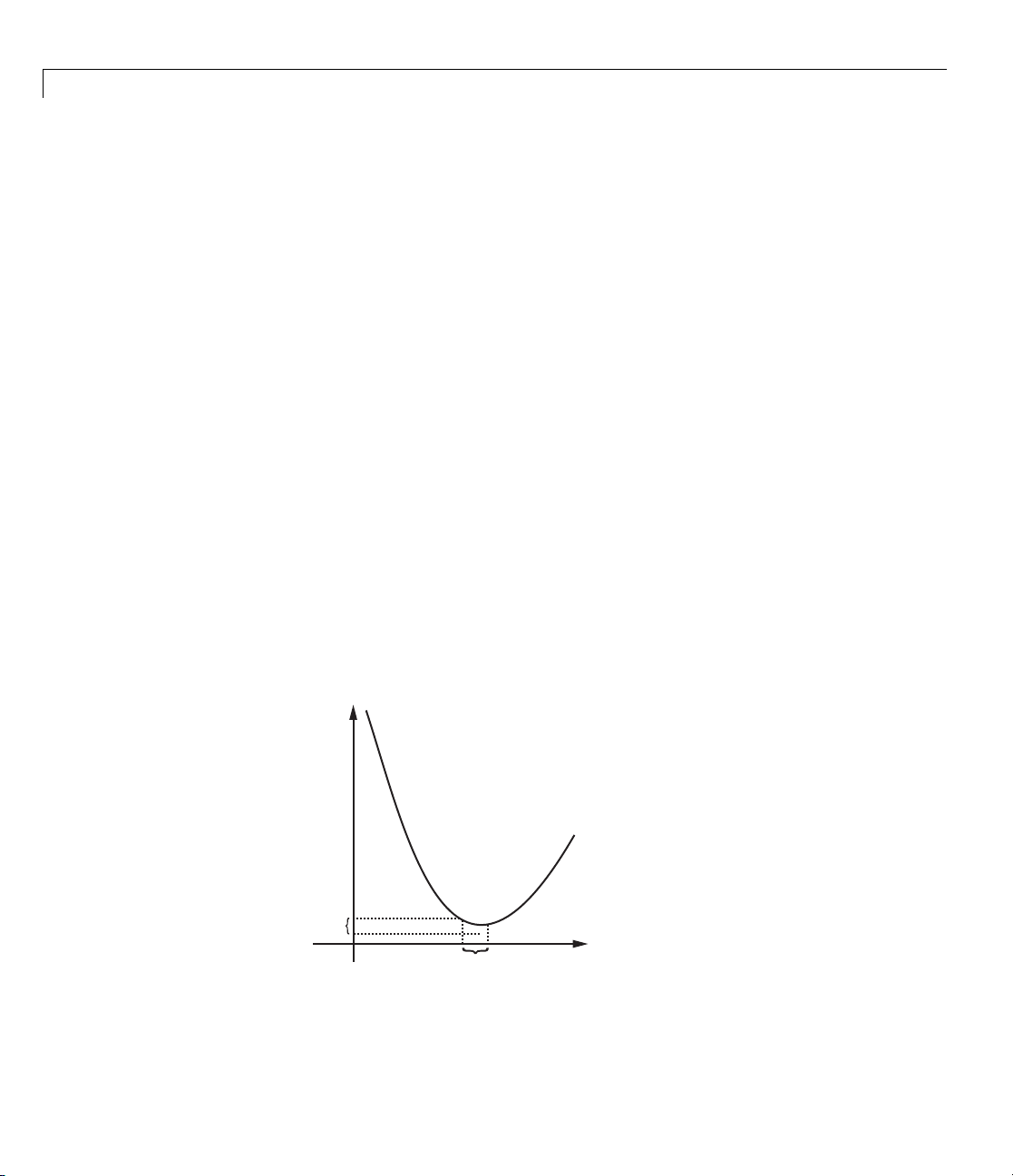
2 Setting Up an Optimization

or

There are several predefined plot f unctions. See the solver function reference
pages for a list, or view a list in the
on page 9-7 table.

Tolerances and Stopping Criteria

The number of iterations in an optimization depends on a solver’s stopping
criteria. These criteria include several tolerances you can set. Genera lly, a

tolerance is a threshold which, if crossed, stops the iterations of a solver.

options = optimset('PlotFcns',@plotfun);

options = optimset('PlotFcns',...

plotfun1,@plotfun2,...});

{@

PlotFcns entry of the “Options Structure”

Set tolerances and other criteria using

optimset as explained in “Setting

Options” on page 2-30.

•

TolX is a lower bound on the size of a step, meaning the norm of (x

the solver attempts to take a step that is smaller than

end.

TolX is sometimes used as a relative bound, meaning iterations end

when |(x

– x

)| < TolX*(1 + |xi|),orasimilarrelativemeasure.

i

i+1

TolX, the iterations

i

– x

i+1

). If

Iterations end
when the last step

1



is smaller than
TolFun or TolX

2



3



4

5



TolFun



TolX

• TolFun is a lower bound on the change in the value of the objective function

during a step. If |f(x

)–f(x

i

)| < TolFun,theiterationsend. TolFun

i+1

2-36

is sometimes used as a relative bound, meaning iterations end when

|f(x

)–f(x

i

TolFun is also a bound on the first-order optimality measure. If the

•

optimality measure is less than

)| < TolFun(1 + |f(xi)|), or a similar relative measure.

i+1

TolFun, the iterations end. TolFun can

also be a relative bound. First-order optimality measure is defined in

“First-Order Optimality Measure” on page 3-11.

•

TolCon is an upper bound on the magnitude of any constraint functions.

Ifasolverreturnsapointx with c(x)>

solver reports that the constraints are violated at x.

TolCon or |ceq(x)| > TolCon,the

TolCon canalsobea

relative bound.

Note TolCon operates differently from other tolerances. If TolCon is not

satisfied (i.e., if the magnitude of the constraint function exceeds

TolCon),

the solver attempts to continue, unless it is halted for another reason. A

solver does not halt simply because

TolCon is satisfied.

Setting Options

• MaxIter is a bound on the number of solver iterations. MaxFunEvals is

a bound on the number of function evaluations. Iterations and function

evaluations are discussed in “Iterations and Function Counts” on page 3-10.

There are two other tolerances that a ppl y to particular solvers:

MaxPCGIter. These relate to preconditioned conjugate gradient steps. For

TolPCG and

more information, see “Preconditioned Conjugate Gradient Method” on page
6-23.

There are several tolerances that apply only to the

fmincon interior-point

algorithm. For more information, see “Optimization Options” on page 9-7.

Checking Validity of Gradients or Jacobians

• “How to Check Derivatives” on page 2-38

• “Best Practices for Checking Derivatives” on page 2-39

• “Example: Checking Derivatives of Objective and Constraint Functions”

on page 2-39

2-37

2 Setting Up an Optimization

Many solvers allow you to supply a function that calculates first derivatives
(gradients or Jacobians) of objective or constraint functions. You can check
whether the derivatives calculated b y your function match finite-difference
approximations. This check can help you diagnose whether your derivative
function is correct.

• If a component of the gradient function is less than

1, “match” means

the absolute difference of the gradient function and the finite-difference

approximation of that component is less than

• Otherwise, “match” means that the relative difference is less than

The

DerivativeCheck option causes the solver to check the supplied

1e-6.

1e-6.

derivative against a finite-difference approximation only at the initial point. If
the finite-difference and supplied derivatives do not match, the solver reports
the discrepancy, and asks whether you want to continue. If the derivatives
match, the solver reports the differences, and continues without asking.

When

DerivativeCheck is 'on' and GradObj or Jacobian is 'on',the

solver compares your objective gradient function against a finite difference
approximation. Similarly, when

DerivativeCheck is 'on' and GradConstr

is 'on', the solver compares your constraint gradient function against a
finite-difference approximation.

Choose an initial point with nonzero, noninteger components when using

DerivativeCheck. Often, gradients match at a simple initial point, but not

at other points. Furthermore, as shown in “Checking Derivatives with the
Optimization Tool” on page 2-42, the small inaccuracy inherent in finite
difference approximations can be e specially problematic at

0 or other integer

components.

2-38

How to Check Derivatives

• At the MATLAB com mand line:

1 Set the

optimset. Make sure your objective or constraint functions supply the

appropriate derivatives.

2 Set the

GradObj, GradConstr,orJacobian options to 'on' with

DerivativeCheck option to 'on'.

Setting Options

• Using the Optimization Tool:

1 In the Problem Setup and Results pane, choose Derivatives:

Objective function:
function: Derivatives:

or constraint functions supply the appropriate derivatives.

2 In the Options pane, check User-supplied derivatives > Validate

user-supplied derivatives

Gradient supplied or Nonlinear constraint

Gradient supplied. Makesureyourobjective

Best Practices for Checking Derivatives

• Choose a random initial point, such as randn(size(x0)).Ifallcomponents

have lower and upper bounds, choose a random point satisfying the bounds:

rand(size(x0)).*(ub-lb) + lb.Herex0 has same size as your initial

vector,

• Use central finite differences (for applicable solvers). These d ifferences are

more accurate than the default forward differences. To do so:

lb is the vector of lower bounds, and ub is the vector of upper bounds.

- At the MATLAB command line, set FinDiffType option to 'central'

with optimset.

- Using the Optimization Tool, in the Approximated derivatives pan e,

set Type to

Example: Checking Derivatives of Objective and Constraint
Functions

• “Objective and Constraint Functions” on page 2-39

• “Checking Derivatives at th e Command Line” on page 2-41

• “Checking Derivatives with the Optimization Tool” on page 2-42

Objective and Constraint Functions. Consider the problem of minimizing

the Rosenbrock function within the unit disk as described in “Example:
Nonlinear Constrained Minimization” on page 1-4. The
calculates the objective function and its gradient:

function [f g H] = rosenboth(x)

central differences.

rosenboth function

2-39

2 Setting Up an Optimization

f = 100*(x(2) - x(1)^2)^2 + (1-x(1))^2;

if nargout > 1

g = [-400*(x(2)-x(1)^2)*x(1)-2*(1-x(1));

200*(x(2)-x(1)^2)];

if nargout > 2

H = [1200*x(1)^2-400*x(2)+2, -400*x(1);

-400*x(1), 200];

end

end

rosenboth

calculates the Hessian, too, but this example does not use the

Hessian.

The

unitdisk2 function correctly calculates the constraint function and its

gradient:

function [c,ceq,gc,gceq] = unitdisk2(x)
c = x(1)^2 + x(2)^2 - 1;
ceq = [ ];

if nargout > 2

gc = [2*x(1);2*x(2)];
gceq = [];

end

The unitdiskb function incorrectly calculates gradient of the constraint
function:

function [c ceq gc gceq] = unitdiskb(x)
c = x(1)^2 + x(2)^2 - 1;
ceq = [ ];

if nargout > 2

gc = [x(1);x(2)]; % Gradient incorrect: off by a factor of 2
gceq = [];

end

2-40

Setting Options

Checking Derivatives at the Command Line.

1 Set the options to use the interior-point algorithm , gradient of objective and

constraint functions, and the

options = optimset('Algorithm','interior-point',...

'DerivativeCheck','on','GradObj','on','GradConstr','on');

DerivativeCheck option:

Setting Algorithm to 'active-set' works, too. Best practice would set

FinDiffType to 'central'.

2 Solve the minimization with fmincon using the erroneous unitdiskb

constraint function:

[x fval exitflag output] = fmincon(@rosenboth,...

[-1;2] + randn(2,1),[],[],[],[],[],[],@unitdiskb,options);
Objective function derivatives:
Maximum relative discrepancy between derivatives = 2.60089e-008
Nonlinear inequality constraint derivatives:
Maximum relative discrepancy between derivatives = 1
Caution: user-supplied and forward finite-difference derivatives

do not match within 1e-006 relative tolerance.

Maximum relative difference occurs in element (1,1):

User-supplied constraint gradient: -3.25885
Finite-difference constraint gradient: -6.51769

Strike any key to continue or Ctrl-C to abort.

The constraint function does no t match the calculated gradient,
encouraging you to check the function for an error.

3 Replace the unitdiskb constraint function with unitdisk2 and run the

minimization again:

[x fval exitflag output] = fmincon(@rosenboth,...

[-1;2] + randn(2,1),[],[],[],[],[],[],@unitdisk2,options);
Objective function derivatives:
Maximum relative discrepancy between derivatives = 3.59821e-008
Nonlinear inequality constraint derivatives:
Maximum relative discrepancy between derivatives = 1.14322e-008

Local minimum found that satisfies the constraints...

2-41

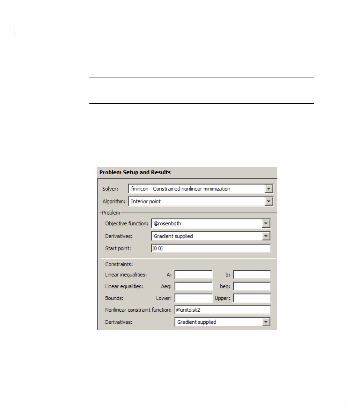
2 Setting Up an Optimization

Checking Derivatives with the Optimization Tool.

Note Take care when using DerivativeCheck with the Optimization Tool.

Ifthederivativecheckfails,thereisno indication in the Optimization Tool.
Check the Command Window to see the message and act, if necessary.

To set up the example using correct derivative functions, but starting from

[0 0], using the Optimization Tool:

1 Launch the Optimization Tool by entering optimtool at the command line.

2 Set the Problem Setup and Results pane to match the following figure:

2-42

3 Set the Options pane to match the following figure:

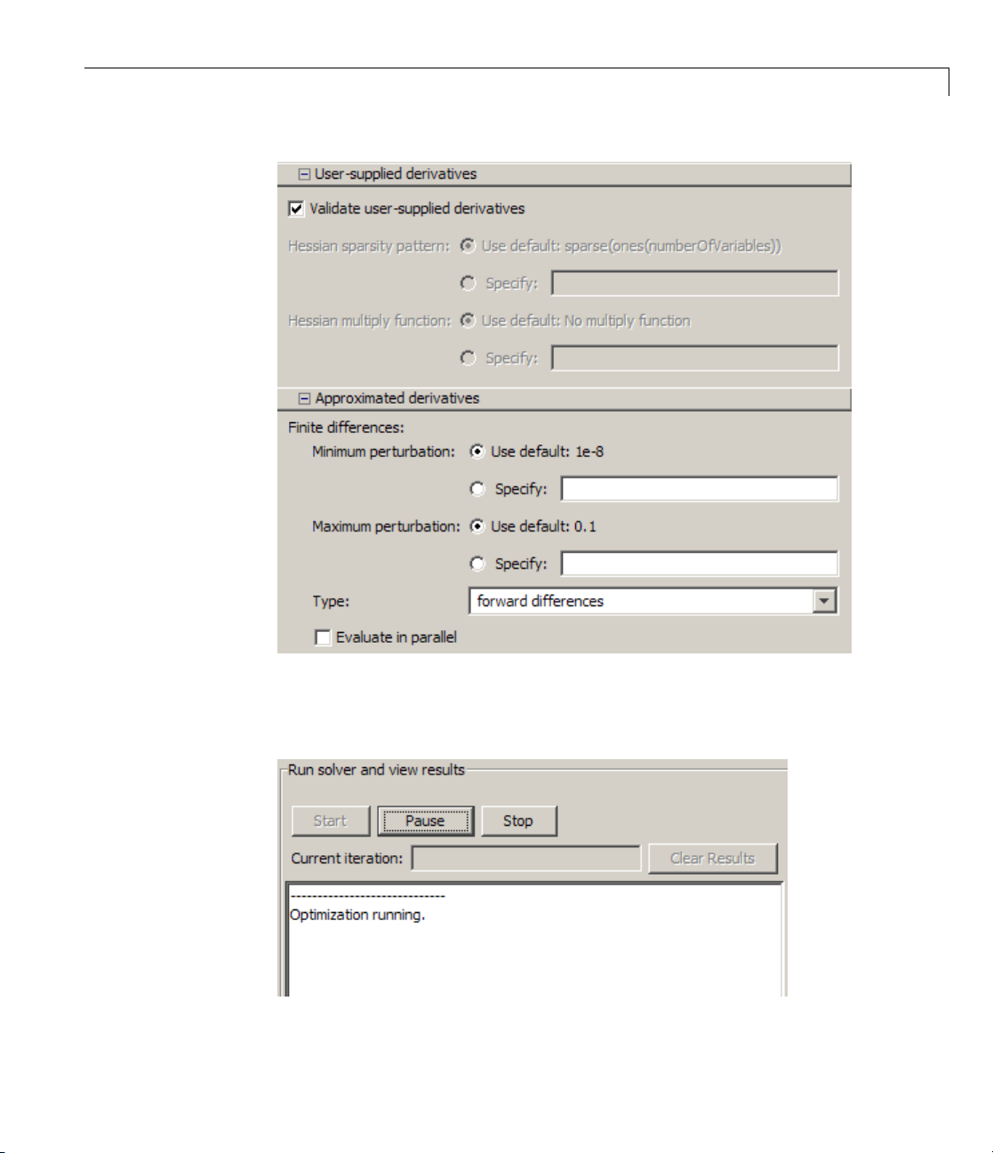
Setting Options

4 Press t

The out

he Start button under Run solver and view results.

put screen displays

2-43

2 Setting Up an Optimization

5 Strike a key in the command window, and the optimization continues to

However, the process does not continue. The MATLAB command window
displays:

Objective function derivatives:
Maximum relative discrepancy between derivatives = 1.49012e-006
Caution: user-supplied and forward finite-difference derivatives

do not match within 1e-006 relative tolerance.

Maximum relative difference occurs in element 2 of gradient:

User-supplied gradient: 0
Finite-difference gradient: 1.49012e-006

Strike any key to continue or Ctrl-C to abort.

The forward finite difference approximation is inaccurate enough at [0

that the derivative check fails.

0]

completion.

2-44

Setting Options

The derivative check succeeds when you select central differences in
the Approximated derivatives > Type pane. The derivative check also
succeeds when you select the initial point

[-1 2], or most random points.

Choosing the Algorithm

• “fmincon Algorithms” on page 2-45

• “fsolve Algorithms” on page 2-46

• “fminunc Algorithms” on page 2-47

• “Least Squares Algorithms” on page 2-48

• “Linear Programming Algorithms” on page 2-49

• “Quadratic Programming Algorithms” on p age 2-50

fmincon Algorithms

fmincon has four algorithm options:

•

'interior-point'

• 'sqp'

• 'active-set'

• 'trust-region-reflective' (default)

Use

optimset to set the Algorithm option at the command line.

Recommendations

• Use the 'interior-point' algorithm first.

For help if the minimization fails, see“WhentheSolverFails”onpage
4-3 or “When the Solver Might Have Succeeded” on page 4-14.

• Torunanoptimizationagaintoobtainmorespeedonsmall-to

medium-sized problems, try

• Use

'trust-region-reflective' when applicable. Your problem must

'sqp' next, and 'active-set' last.

have: objective function includes gradient, only bounds, or only linear
equality constraints (but not both).

2-45

2 Setting Up an Optimization

Reasoning Behind the Recommendations.

•

•

•

•

'interior-point' handles large, sparse problems, as well as small dense

problems. The algorithm satisfies bounds at all iterations, and can recover
from

NaN or Inf results. It is a large-scale algorithm; see “Large-Scale

vs. Medium-Scale Algorithms” on page 2-35. The algorithm can use
special techniques for large-scale problems. For details, see “Interior-Point
Algorithm” on page 11-56.

'sqp' satisfies bou nd s at all iterations. Th e algorithm can recover from
NaN or Inf results. It is not a large-scale algorithm ; see “Large-Scale vs.

Medium-Scale Algorithms” on page 2-35.

'active-set' can take large steps, which adds speed. The algorithm

iseffectiveonsomeproblemswithnonsmooth constraints. It is not a
large-scale algorithm; see “Large-Scale vs. Medium-Scale Algorithms”
on page 2-35.

'trust-region-reflective' requires you to provide a gradient, and

allows only bounds or linear equality constraints, but not both. Within
these limitations, the algorithm handles both large sparse problems
and small dense problems efficie n t ly. It is a large-scale algorithm; see
“Large-Scale vs. Medium-Scale Algorithms” on page 2-35. The algorithm
can use special technique s to save memory usage, such as a Hessian
multiply function. For details, see “Trust-Region-Reflective Algorithm” on
page 11-53.

2-46

- 'trust-region-reflective' is the default algorithm for historical

reasons. It is effective when applicable, but it has many restrictions,
so is not always applicable.

fsolve Algorithms

fsolve has three algorithms:

•

'trust-region-dogleg' (default)

'trust-region-reflective'

•

• 'levenberg-marquardt'

Use optimset to set the Algorithm option at the command line.

Recommendations

• Use the 'trust-region-dogleg' algorithm first.

Setting Options

For help if

fsolve fails, see “When the Solver Fails” on page 4-3 or

“When the Solver Might Have Succeeded” on page 4-14.

• To solve equations again if you have a Jacobian multiply function,

or want to tune the internal algorithm (see “Trust-Reg io n-Re flectiv e
Algorithm Only” on p age 11-126), try

• Try timing all the algorithms, including

'trust-region-reflective'.

'levenberg-marquardt',tofind

the algorithm that works b est on your problem.

Reasoning Behind the Recommendations.

•

'trust-region-dogleg' is the only algorithm that is specially designed

to solve nonlinear equations. The others attempt to minimize the sum
of squares of the function.

• The

'trust-region-reflective' algorithm is effective on sparse

problems. It can use special techniques such as a Jacobian multiply
function for large-scale problems.

fminunc Algorithms

fminunc has two algorithms:

• Large-scale

• Medium-scale

Choose between them at the command line by using

LargeScale option to:

•

'on' (default) for Large-scale

'off' for Medium-scale

•

optimset to set the

2-47

2 Setting Up an Optimization

Recommendations

• If your objective function includes a gradient, use 'LargeScale' = 'on'.

• Otherwise, use

'LargeScale' = 'off'.

For he lp if the minimization fails, see “When the Solver Fails” on page 4-3
or “When the Solver Might Have Succe eded” on page 4-14.

Least Squares Algorithms

lsqlin. lsqlin has two algorithms:

• Large-scale

• Medium-scale

Choose between them at the command line by using

LargeScale option to:

•

'on' (default) for Large-scale

'off' for Medium-scale

•

Recommendations

• If you have no constraints or only bound constraints, use

'LargeScale' = 'on'.

• If you have linear constraints, use

'LargeScale' = 'off'.

optimset to set the

2-48

For he lp if the minimization fails, see “When the Solver Fails” on page 4-3
or “When the Solver Might Have Succe eded” on page 4-14.

lsqcurvefit and lsqnonlin. lsqcurvefit and lsqnonlin have two
algorithms:

•

'trust-region-reflective' (default)

'levenberg-marquardt'

•

Use optimset to set the Algorithm option at the command line.

Setting Options

Recommendations

• If you have no constraints or only bound constraints, use

'trust-region-reflective'.

• If your problem is underdetermined (fewer equations than dimensions),

use

'levenberg-marquardt'.

For he lp if the minimization fails, see “When the Solver Fails” on page 4-3
or “When the Solver Might Have Succe eded” on page 4-14.

Linear Programming Algorithms

linprog has three algorithms:

• Large-scale interior-point

• Medium-scale active set

• Medium-scale Simplex

Choose between them at the command line by using

LargeScale option to:

•

'on' (default) for large-scale interior-point

'off' for one of the other tw o

•

When
by setting the

LargeScale is 'off', choose between the two remaining algorithms

Simplex option to:

optimset to set the

- 'on' for Simplex

- 'off' (default) for active set

Recommendations

Use 'LargeScale' = 'on'

For he lp if the minimization fails, see “When the Solver Fails” on page 4-3
or “When the Solver Might Have Succe eded” on page 4-14.

2-49

2 Setting Up an Optimization

Quadratic Programming Algorithms

quadprog has two algorithms:

• Large-scale

• Medium-scale

Choose between them at the command line by using

LargeScale option to:

•

'on' (default)

'off'

•

Recommendations

• If you have only b ounds, or only linear equalities, use

'LargeScale' = 'on'.

• If you have linear inequalities, or both bounds and linear equalities,

use

'LargeScale' = 'off'.

For he lp if the minimization fails, see “When the Solver Fails” on page 4-3
or “When the Solver Might Have Succe eded” on page 4-14.

optimset to set the

2-50

Examining Results

• “Current Point and Function Value” on page 3-2

• “Exit Flags and Exit Messages” on page 3-3

• “Iterations and Function Counts” on page 3-10

• “First-Order Optimality Measure” on page 3-11

• “Displaying Iterative Output” on page 3-14

• “Output Structures” on page 3-21

• “Lagrange Multiplier Structures” on page 3-22

3

• “Hessian” on page 3-23

• “Plot Functions” on page 3-26

• “Output Functions” on page 3-32

3 Examining Results

Current Point and Function Value

The current point and function value are the first two outputs of all
Optimization Toolbox solvers.

• The current point is the final p oint in the solver iterations. It is the best

point the solver found in its run.

- If you call a solver without assigningavaluetotheoutput,thedefault

output,

• The function value is the value of the objective function at the current point.

ans, is the current point.

- Thefunctionvalueforleast-squares solvers is the sum of squares, also

known as the residual norm.

- fgoalattain, fminimax,andfsolve return a vector function value.

- Sometimes fval or Fval denotes function value.

3-2

Exit Flags and Exit Messages

In this section...

“ExitFlags”onpage3-3

“Exit Messages” on page 3-5

“Enhanced Exit Messages” on page 3-5

“Exit Message Options” on page 3-8

Exit Flags

When an optimization solver co mplete s its task, it sets an exit flag.Anexit
flag is an integer that is a code for the reason the s olver halted i ts iterations.
In general:

• Positive exit flags correspond to successful outcomes.

• Negative exit flags correspond to unsuccessful outcomes.

Exit Flags and Exit Messages

• The zero exit flag corresponds to the solver being halted by exceeding

an iteration limit or limit on the number of function evaluations (see
“Iterations and Function Counts” on page 3-10, and also see “Tolerances
and Stopping Criteria” on page 2-36).

A table of solver outputs in the solver’s function reference section lists the
meaning of each solver’s exit flags.

Note Exit flags are not infallible guides to the quality of a solution. Many
other factors, such as tolerance settings, can affect whether a solution is
satisfactory to you. You are responsible for deciding whether a solver returns
a satisfactory answer. Sometimes a negative exit flag does not correspond to a
“bad” solution. Similarly, sometimes a positive exit flag does not correspond
to a “good” solution.

Youobtainanexitflagbycallingasolverwiththeexitflag syntax. This
syntax depends on the solver. For details, see the solver function reference
pages. For example, for

fsolve,thecallingsyntaxtoobtainanexitflagis

3-3

3 Examining Results

[x,fval,exitflag] = fsolve(...)

The following example uses this syntax. Suppose you want to solve the system
of nonlinear equations

x

−

2

xx e

−=

12

2

xxe

−+ =

12

1

x

−

2

.

Write these equations as an anonymous function that gives a zero vector
at a solution:

myfcn = @(x)[2*x(1) - x(2) - exp(-x(1));

-x(1) + 2*x(2) - exp(-x(2))];

Call fsolve with the exitflag syntax at the initial point [-5 -5]:

[xfinal fval exitflag] = fsolve(myfcn,[-5 -5])

3-4

Equation solved.

fsolve completed because the vector of function values is near
zero as measured by the default value of the function tolerance,
and the problem appears regular as measured by the gradient.

xfinal =

0.5671 0.5671

fval =

1.0e-006 *

-0.4059

-0.4059

exitflag =

1

In the table for fsolve under “Output Arguments” on page 11-91, you find
that an exit flag value
words,

fsolve reports myfcn is nearly zero at x = [0.5671 0.5671].

1 means “Function converged to a solution x.” In other

Exit Flags and Exit Messages

Exit Messages

Each solver issues a message to the MATLAB command window at the end
of its iterations. This message explains briefly why the solver halted. The
message might give more detail than the exit flag.

Many examples in this documentation show exit messages. For example, see
“Minimizing at the Command Line” on page 1-11, or “Step 2: Invoke one of
the unconstrained optimization routines.” on page 6-14. The example in the
previous section, “Exit Flags” on page 3-3, shows the following exit message:

Equation solved.

fsolve completed because the vector of function values is near
zero as measured by the default value of the function tolerance,
and the problem appears regular as measured by the gradient.

Thismessageismoreinformativethantheexitflag. Themessageindicates
that the gradient is relevant. The message also states that the function
tolerance controls how near 0 the vector of function values must be for
to regard the solution as completed.

fsolve

Enhanced Exit Messages

Some solvers have exit messages that contain links for more information.
Therearetwotypesoflinks:

• Links on words or phrases. If you click such a link, a window opens that

displays a definition of the term, or gives other information. The new
window can contain links to the Help browser documentation for more
detailed information.

• A link as the last li ne of the display saying <stopping criteria details>. If

you click this link, MATLAB displays more detail about the reason the
solver halted.

The

fminunc solver has enhanced exit messages:

opts = optimset('LargeScale','off'); % LargeScale needs gradient
[xfinal fval exitflag] = fminunc(@sin,0,opts)

This yields the following results:

3-5

3 Examining Results

3-6

Each of the underlined words or phrase s contains a link that provides more
information.

• The

<stopping criteria details> link prints the following to the

MATLAB command line:

Optimization completed: The first-order optimality measure, 0.000000e+000, is less

than the default value of options.TolFun = 1.000000e-006.

Optimization Metric User Options

relative norm(gradient) = 0.00e+000 TolFun = 1e-006 (default)

• The other links bring up a help window with term definitions. For example,

clicking the

Local minimum found link opens the following window:

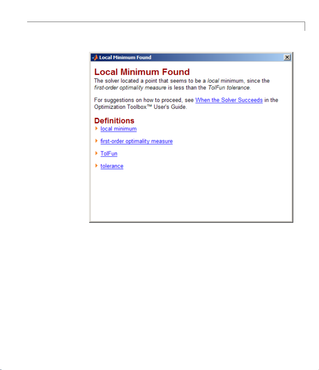
Exit Flags and Exit Messages

Clicking the first-order optimality measure expander link brings up
the d efinition of first-order optimality measure for

fminunc:

3-7

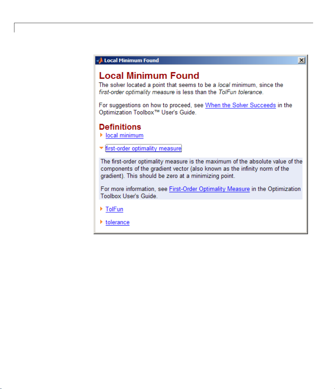
3 Examining Results

3-8

Theexpanderlinkisawaytoobtainmoreinformationinthesamewindow.
Clicking the
closes the definition.

• The other links open the Help Viewer.

first-order optimality measure expander link again

Exit Message Options

Set the Display option to control the appearance of both exit messages and
iterative display. For more information, see “Displaying Iterative Output” on
page 3-14. The following table shows the effect of the various settings of the

Display option.

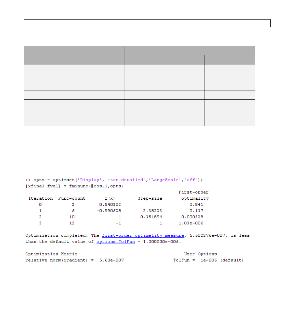
Exit Flags and Exit Messages

Value of the Display Opti on

Output to Command Window

Exit message

'none', or the synonymous 'off'

'final' (default for most solvers) Default

'final-detailed'

'iter'

'iter-detailed'

'notify'

'notify-detailed'

None None

Detailed

Default

Detailed

Default only if exitflag ≤ 0

Detailed only if exitflag ≤ 0

For example,

opts = optimset('Display','iter-detailed','LargeScale','off');
[xfinal fval] = fminunc(@cos,1,opts);

yields the following display:

Iterative Display

None

None

Yes

Yes

None

None

3-9

3 Examining Results

Iterations and Function Counts

In general, Optimization Toolbox solvers iterate to find an optimum. This
means a solver begins at an initial value x
calculations that eventually lead to a new point x
process to find successiv e approximation s x
Processing stops after some number of iterations k.

At any step, intermediate calculations may involve evaluating the objective
function and constraints, if any, at points near the current iterate x
example, the solver may estimate a gradient by finite differences. At each of
these nearby points, the function count (

, performs some intermediate

0

2

F-count) is increased by one.

,andthenrepeatsthe

1

, x3, ... of the local minimum.

.For

i

• If there are no constraints, the

F-count reports the total number of

objective function evaluations.

• If there are constraints, the

F-count reports only the number of points

where function evaluations took place, not the total number of evaluations
of constraint functions.

• If there are many constraints, the

F-count can be significantly less than

the total number of function evaluations.

F-count is a header in the iterative display for many solvers. For an example,

see “Interpreting the Result” on page 1-12.

The

F-count appears in the output structure as output.funcCount.This

enables you to access the evaluation count programmatically. For more
information on output structures, see “Output Structures” on page 3-21.

Sometimes a solver attempts a step, and rejects the attempt. The

trust-region-reflective,andtrust-region-dogleg algorithms

LargeScale,

count these failed attempts as iterations, and report the (unchanged)
result in the iterative display. The

levenberg-marquardt algorithms do not count such an attempt as an

interior-point, active-set,and

iteration, and do not report the attempt in the iterative display. All attempted
steps increase the

F-count, regardless of the algorithm.

3-10

First-Order Optimality Measure

First-order optimality is a measure of how close a point x is to optimal. It
is used in all smooth solvers, constrained and unconstrained, though it
has different meanings depending on the problem and solver. For more
information about first-order optimality, see Nocedal and Wright [31].

First-Order Optimality Measure

The tolerance
optimality measure is less than

TolFun relates to the first-order optimality measure. If the

TolFun, the solver iterations will en d.

Unconstrained Optimality

For a smooth unconstrained problem,

min ( ),xfx

the optimality measure is the infinity-norm (i.e., maxi m um absolute value)
of ∇f(x):

First-order optimality measure = max ( ) ( ) .

This mea
functio
proble
functi
minimi
funct

Const

The t
cons
func

sure of optimali ty is based on the familiar condition for a smooth

n to achieve a minimum: its gradient must be zero. For unconstrained

ms, when the first-order o ptimality measure is nearly zero, the objective

on has gradient nearly zero, so the objective function could be nearly

zed. If the first-order optimality measureisnotsmall,theobjective

ion is n ot minimized.

rained Optimality—Theory

heory behind the definition of first-order optimality measure for
trained problems. The definition as used in Optimization Toolbox
tionsisin“ConstrainedOptimality in Solver Form” on page 3-13.

fx fx∇∇

()

i

=

i

∞

a smooth constrained problem let g and h be vector functions representing

For

inequality and equality constraints respectively (i.e., bou nd, linear, and

all

linear constraints):

non

min ( ) ( ) , ( ) .

fx gx hx subject to ≤=00

x

3-11

3 Examining Results

The m eaning of first-order optimality in this case is more involved than for
unconstrained problems. The definition is based on the Karush-Kuhn-Tucker
(KKT) conditions. The KKT conditions are analogous to the condition that
the gradient must be zero at a minimum, modified to take constraints into
account. The difference is that the KKT conditions hold for constrained
problems.

The KKT conditions are given via an auxiliary Lagrangian function

Lx f x g x h x

(, ) () () ().



=+ +

gi i hi i

,,

∑∑

(3-1)

The vector λ, which is the concatenation of λ
multiplier vector. Its length is the total number of constraints.

The KKT conditions are:

∇xLx(, ) ,



⎧
⎪

⎨
⎪

⎩

The three expressions in Equation 3-4 are not used in the calculation of
optimality measure.

The optimality measure associated with Equation 3-2 is

The optimality measure associated with Equation 3-3 is



= 0

gx i

() ,=∀0

gi i

,

gx

() ,

≤

0

hx

() ,

=

0

≥



∇∇ ∇ ∇

.

0

gi

,

Lx f x g x h x(, () () ().



x gi i hi hi

=+ +

,,,

∑∑

and λh, is called the Lagrange

g





gx

(),

g

(3-2)

(3-3)

(3-4)

(3-5)

(3-6)

3-12

where the infinity norm (maximum) is used for the vector





gi i

gx,()

.

First-Order Optimality Measure

Thecombinedoptimalitymeasureisthemaximumofthevaluescalculatedin
Equation 3-5 and Equation 3-6. In solvers that accept nonlinear constraint
functions, constraint violations g(x)>0or|h(x)|>0aremeasuredand
reported as tolerance violations; see “Tolerances and Stopping Criteria” on
page 2-36.

Constrained Optimality in Solver Form

The first-order optimality measure used by toolbox solvers is expressed as
follows for constraints given separately by bounds, linear functions, and
nonlinear functions. The measure is the maximum of the following two norms,
which correspond to Equation 3-5 and Equation 3-6:

∇∇

Lx f x A Aeq(, ()



x

=+ +

+++

  

lx xu

−−



iiloweriiiupperi

,

,,

T

ineqlin



ineqnonlin i i eqnonlin i i

  

,,

,( ) , ( )

T

eqlin

c x ceq x

() (),∇∇

∑∑



Ax b c x

−



i ineqlin i i ineqno

,

nnlin i,

(3-7)

,

(3-8)

where the infinity norm (maximum) is used for the vector in Equation 3-7 and
in Equation 3-8. The subscripts on the Lagrange multipliers correspond to
solver Lagrange multiplier structures; see “Lagrange Multiplier Structures”
on page 3-22. The summations in Equation 3-7 range over all constraints. If
a bound is ±

Inf, that term is not co nsidered constrained, so is not part of

the summation.

For some large-scale problems with only linear equalities, the first-order
optimality measure is the infinity norm of the projected gradient (i.e., the
gradient projected onto the nullspace of

Aeq).

3-13

3 Examining Results

Displaying Iterative Output

In this section...

“Introduction” on page 3-14

“Most Common Output Headings” on page 3-14

“Function-Specific Output Headings” on page 3-15

Note An optimization function does not return all of the output headings,
described in the following tables, each time you call it. Which output headings
are returned depends on the algorithm the optimization function uses for
a particular problem.

Introduction

When you set 'Display' to 'iter' or 'iter-detailed' in options,the
optimization functions display iterative output in the Command Window.
This output, which provides information about the progress of the algorithm,
is displayed in columns with descriptive headings. For more information
about iterations, see “Iterations and Function Counts” on page 3-10.

3-14

For example, if you run medium-scale
the output headings are

Iteration Func-count f(x) Step-size optimality

fminunc with 'Display' set to 'iter',

First-order

Most Common Output Headings

The following table lists some common output headings of iterative output.

Outp

ration

Ite

nc-count

Fu

count

F-

ut Heading

or Iter

or

rmation Displayed

Info

ration number; see “Iterations and Function

Ite

nts” on page 3-10

Cou

mber of function evaluations; see “Iterations

Nu

d Function Counts” on page 3-10

an

Displaying Iterative Output

Output Heading Information Displayed

x

f(x)

Step-size

Norm of step

Current point for the algorithm

Current function value

Step size in the current search direction

Norm of the current step

Function-Specific Output Headings

The following sections describe output headings of iterative output whose
meaning is specific to the optimization function you are using.

• “bintprog” on page 3-15

• “fminsearch” on page 3-16

• “fzero and fminbnd” on p ag e 3-17

• “fminunc” on page 3-17

• “fsolve” on page 3-18

• “fgoalattain, fmincon, fminimax, and fseminf” on page 3-18

• “linprog” on page 3-19

• “lsqnonlin and lsqcurvefit” on page 3-20

bintprog

The following table describes the output headings specific to bintprog.

bintprog
Output
Heading Information Displayed

Explored
nodes

Obj of LP
relaxation

Cumulative number of explored nodes

Objective function value of the linear programming (LP)
relaxation problem

3-15

3 Examining Results

bintprog
Output
Heading Information Displayed

Obj of best
integer point

Objective function value of the best integer point found
so far. This is an upper bound for the final objective
function value.

Unexplored
nodes

Best lower
bound on obj

Number of nodes that have been set up but not yet
explored

Objective function value of LP relaxation problem that
gives the best current lower bound on the final objective
function value

Relative
gap between
bounds

1001()

ba

b−+

,

where

• b is the objective function value of the b est integer

point.

3-16

• a is the best lower bound on the o bjectiv e function

value.

fminsearch

The following table describes the output headings specific to fminsearch.

fminsearch
Output
Heading Information Displayed

min f(x)

Procedure

Minimum function value in the current simplex

Simplex p rocedure at the current iteration. Procedures
include

inside

initial, expand, reflect, shrink, contract

,andcontract outside. See “fminsearch
Algorithm” on page 6-11 for explanations of these
procedures.

Displaying Iterative Output

fzero and fminbnd

The following table des cribes the output headings specific to fzero and

fminbnd.

fzero and
fminbnd
Output
Heading Information Displayed

Procedure

Procedure at the current operation. Procedures for

fzero:

•

initial (initial point)

search (search for an interval containing a zero)

•

bisection (bisection search)

•

interpolation

•

Operations for fminbnd:

•

initial

• golden (golden section search)

parabolic (parabolic interpolation)

•

fminunc

The following table describes the output headings specific to fminunc.

fminunc
Output
Heading Information Displayed

First-order
optimality

CG-iterations

First-order optimality measure (see “First-Order
Optimality Measure” on page 3-11)

Number of conjugate gradient iterations taken by the
current (optimization) iteration (see “Preconditioned
Conjugate Gradient Method” on page 6-23)

3-17

3 Examining Results

fsolve

The following table describes the output headings specific to fsolve.

fsolve Output
Heading Information Displayed

First-order
optimality

Trust-region
radius

Residual

Directional
derivative

First-order optimality measure (see “First-Order
Optimality Measure” on page 3-11)

Current trust-region radius (change in the norm of the
trust-region radius)

Residual (sum of squares) of the function

Gradient of the function along the search direction

fgoalattain, fmincon, fminimax, and fseminf

The following table describes the output headings specific to fgoalattain,

fmincon, fminimax,andfseminf.

3-18

fgoalattain,
fmincon,
fminimax, fseminf
Output Heading Information Displayed

Max constraint

Maximum violation among all constraints, both
internally constructed and user-provided

First-order
optimality

CG-iterations

First-order optimality measure (see “First-Order
Optimality Measure” on page 3-11)

Number of conjugate gradient iterations taken by the
current (optimization) iteration (see “P r econditioned
Conjugate Gradient Method” on page 6-23)

Trust-region
radius

Residual

Attainment factor

Current trust-region radius

Residual (sum of squares) of the function

Value of the attainment factor for fgoalattain

Displaying Iterative Output

fgoalattain,
fmincon,
fminimax, fseminf
Output Heading Information Displayed

Objective value

Objective function value of the nonlinear
programming reformulation of the minimax problem
for

fminimax

Directional
derivative

Procedure

Current gradient of the function along the search
direction

Hessian update and QP subproblem. The Procedure
messages are discuss ed in “Updating the Hessian
Matrix” on page 6-29.

linprog

The following table describes the output headings specific to linprog.

linprog Output
Heading Information Displayed

Primal Infeas
A*x-b

Dual Infeas
A'*y+z-w-f

Duality Gap
x'*z+s'*w

Primal infeasibility

Dual infeasibility

Duality gap (see “Large Scale Linear Programming” on
page 6-91) between the primal objective and the dual
objective.

s and w appear only in this equation if there

are finite upper bou n ds.

Total Rel
Error

Objective f'*x

Total relative error, described at the end of “Main
Algorithm” on page 6-91.

Current objective value

3-19

3 Examining Results

lsqnonlin and lsqcurvefit

The following table describes the output headings specific to lsqnonlin and

lsqcurvefit.

lsqnonlin and
lsqcurvefit
Output
Heading Information Displayed

Resnorm

Residual

First-order
optimality

CG-iterations

Directional
derivative

Lambda

Valueofthesquared2-normoftheresidualatx

Residual vector of the function

First-order optimality measure (see “First-Order
Optimality Measure” on page 3-11)

Number of conjugate gradient iterations taken by the
current (optimization) iteration (see “Preconditioned
Conjugate Gradient Method” on page 6-23)

Gradient of the function along the search direction

λkvalue d efined in “Levenberg-Marquardt Method” on

page 6-139. (This value is displayed w hen you use the
Levenberg-Marquardt method and omitted when you
use the Gauss-Newton method.)

3-20