Mathworks IMAGE PROCESSING TOOLBOX 7 user guide

Download

Image Processing T

User’s Guide

oolbox™ 7

How to Contact The MathWorks

www.mathworks. comp.soft-sys.matlab Newsgroup www.mathworks.com/contact_TS.html T echnical Support

suggest@mathworks.com Product enhancement suggestions bugs@mathwo doc@mathworks.com Documentation error reports service@mathworks.com Order status, license renewals, passcodes info@mathwo

com

rks.com

Web

Bug reports

Sales, prici

ng, and general information

508-647-7000 (Phone)

508-647-7001 (Fax)

The MathWorks, Inc. 3 Apple Hill Drive Natick, MA 01760-2098

For contact information about worldwide offices, see the MathWorks Web site.

Image Processing Toolbox™ User’s Guide

The software described in this document is furnished under a license agreement. The software may be used or copied only under the terms of the license agreement. No part of this manual may be photocopied or reproduced in any form without prior written consent from The MathW orks, Inc.

FEDERAL ACQUISITION: This provision applies to all acquisitions of the Program and Documentation by, for, or through the federal government of the United States. By accepting delivery of the Program or Documentation, the government hereby agrees that this software or documentation qualifies as commercial computer software or commercial computer software documentation as such terms are used or defined in FAR 12.212, DFARS Part 227.72, and DFARS 252.227-7014. Accordingly, the terms and conditions of this Agreement and only those rights specified in this Agreement, shall pertain to and govern theuse,modification,reproduction,release,performance,display,anddisclosureoftheProgramand Documentation by the federal government (or other entity acquiring for or through the federal government) and shall supersede any conflicting contractual terms or conditions. If this License fails to meet the government’s needs or is inconsistent in any respect with federal procurement law, the government agrees to return the Program and Docu mentation, unused, to The MathWorks, Inc.

Trademarks

MATLAB and Simulink are registered trademarks of The MathWorks, Inc. See

www.mathworks.com/trademarks for a list of additional trademarks. Other product or brand

names may be trademarks or registered trademarks of their respective holders.

Patents

The MathWorks products are protected by one or more U.S. patents. Please see

www.mathworks.com/patents for more information.

Revision History

August 1993 First printing Version 1 May 1997 Second printing Version 2 April 2001 Third printing Revised for Version 3.0 June 2001 Online only Revised for Version 3.1 (Release 12.1) July 2002 Online only Revised for Version 3.2 (Release 13) May 2003 Fourth printing Revised for Version 4.0 (Release 13.0.1) September 2003 Online only Revised for Version 4.1 (Release 13.SP1) June 2004 Online only Revised for Version 4.2 (Release 14) August 2004 Online only Revised for Version 5.0 (Release 14+) October 2004 Fifth printing Revised for Version 5.0.1 (Release 14SP1) March 2005 Online only Revised for Version 5.0.2 (Release 14SP2) September 2005 Online only Revised for Version 5.1 (Release 14SP3) March 2006 Online only Revised for Version 5.2 (Release 2006a) September 2006 Online only Revised for Version 5.3 (Release 2006b) March 2007 Online only Revised for Version 5.4 (Release 2007a) September 2007 Online only Revised for Version 6.0 (Release 2007b) March 2008 Online only Revised for Version 6.1 (Release 2008a) October 2008 Online only Revised for Version 6.2 (Release 2008b) March 2009 Online only Revised for Version 6.3 (Release 2009a) September 2009 Online only Revised for Version 6.4 (Release 2009b) March 2010 Online only Revised for Version 7.0 (Release 2010a)

Getting Started

Product Overview ................................. 1-2

Introduction Configuration Notes Related P roducts Compilability

...................................... 1-2

............................... 1-3

.................................. 1-3

..................................... 1-3

Contents

Example 1 — R eading and Writing Images

Introduction Step 1: Read and Display a n Image Step 2: Check How the Image Appears in the Workspace Step 3: Improve Image Contrast Step4:WritetheImagetoaDiskFile Step 5: Check the Contents of the Newly Written File

Example 2 — A nalyzing Images

Introduction Step 1: Read Image Step 2: Use Morphological Opening to Estimate the

Background

Step 3: View the Background Approximation as a

Surface

Step 4: Subtract the Background Image from the Original

Image Step 5: Increase the Image Contrast Step 6: Threshold the Image Step 7: Identify Objects in the Image Step 8: Examine One Object Step 9: View All Objects Step 10: Compute Area of Each Object Step 11: Compute Area-based Statistics Step 12 : Create Histogram of the Area

...................................... 1-4

................... 1-4

..................... 1-6

..................... 1-11

...................................... 1-12

................................ 1-12

.................................... 1-12

........................................ 1-13

......................................... 1-14

.................. 1-15

........................ 1-16

................. 1-16

......................... 1-17

............................ 1-18

........... 1-4

................ 1-8

................ 1-19

............... 1-20

................ 1-21

.. 1-5

.... 1-9

Getting Help

Product Do c umentation

...................................... 1-22

............................ 1-22

Image Processing Demos ........................... 1-22

MATLAB Newsgroup

.............................. 1-23

Image Credits

..................................... 1-24

Introduction

Images in MATLAB ................................ 2-2

Image Coordinate Systems

Pixel Coordinates Spatial Coordinates Using a Non-Default Spatial Coordinate System

Image Types in the Toolbox

Overview o f Image Types Binary Images Indexed Images Grayscale Images Truecolor Images

Converting Between Image Types

................................. 2-3

................................ 2-4

.................................... 2-8

................................... 2-9

................................. 2-11

.................................. 2-12

......................... 2-3

........ 2-5

........................ 2-7

........................... 2-7

................... 2-16

vi Contents

Converting Between Image Classes

Overview of Image Class Conversions LosingInformationinConversions Converting Indexed Images

Working with Image Sequences

Overview of Toolbox Functions That Work with Image

Sequences Example: Processing Image Sequences Multi-Frame Image Arrays

Image A rithmetic

Overview of Image Arithmetic Functions

..................................... 2-20

.................................. 2-26

......................... 2-18

......................... 2-24

................. 2-18

................... 2-18

..................... 2-20

................ 2-23

.............. 2-26

Image Arithmetic Saturation Rules ................... 2-27

Nesting Calls to Image Arithmetic Functions

........... 2-27

Reading and Writing Image Data

Getting Information About a Graphics File .......... 3-2

Reading Image Data

Writing Image Data to a File

Overview Specifying Format-Specific Parameters ReadingandWritingBinaryImagesin1-BitFormat Determining the Storage Class of the Output File

Converting Between Graphics File Formats

Working with DICOM Files

Overview o f DICOM Support Reading Metadata from a DICOM File Reading Image Data from a DICOM File Writing Image Data or Metadata to a DICOM File

Working with Mayo Analyze 7.5 Files

Working with Interfile Files

Working w ith High Dynamic Range Images

Overview Reading a High Dynamic Range Image Creating a High Dynamic Ran ge Image Viewing a High Dy na m i c Range Ima ge Writing a High Dyna m i c Range Ima ge to a File

........................................ 3-5

........................................ 3-21

............................... 3-3

........................ 3-5

................ 3-6

......................... 3-9

........................ 3-9

................ 3-10

.............. 3-12

................ 3-19

........................ 3-20

................ 3-21

............... 3-22

................ 3-22

.... 3-6

....... 3-7

.......... 3-8

...... 3-13

.......... 3-21

......... 3-23

vii

Displaying and Exploring Images

Overview ......................................... 4-2

Displaying Images Using the imshow Function

Overview Specifying the Initial Image Magnification Controlling the Appearance of the Figure Displaying Each Image in a Separate Figure Displaying Multiple Images in the Same Figure

Using the Image Tool to Explore Images

Image Tool Overview Opening the Image Tool Specifying the Initial Image Magnification Specifying the Colormap Importing Image Data from the Workspace Exporting Image Data to the Workspace Saving the Image Data Displayed in the Image Tool Closing the Image Tool Printing the Image in the Image Tool

Exploring Very Large Images

Overview Creating an R-Set File Opening a n R-Set File

........................................ 4-4

............. 4-6

.............. 4-6

........... 4-7

............. 4-11

.............................. 4-11

............................ 4-13

............. 4-14

............................ 4-15

............ 4-17

............... 4-18

............................. 4-20

................. 4-20

....................... 4-21

........................................ 4-21

............................. 4-21

.............................. 4-21

....... 4-4

........ 4-8

..... 4-18

viii Contents

Using Image Tool Navigation Aids

Navigating a n Image Using the Overview Tool Panning the Image Displayed in the Image Tool ZoomingInandOutonanImageintheImageTool Specifying the Magnification of the Image

GettingInformationaboutthePixelsinanImage

Determining the Value of Individual Pixels Determining the Values of a Group of Pixels Determining the Display Range of an Image

Measuring the Distance Between Two Pixels

.................. 4-23

......... 4-23

........ 4-26

............. 4-27

............ 4-30

........... 4-32

........... 4-35

......... 4-37

..... 4-27

.... 4-30

Using the Distance Tool ............................ 4-37

Exporting Endpoint and Distance Data Customizing the Appearance of the Distance Tool

Getting Information About an Image Using the Image

Information Tool

Adjusting Image Contrast Using the Adjust Contrast

Tool

Understanding Contrast Adjustment Starting the Adjust Contrast Tool Using the Histogram W indow to Adjust Image Contrast Using the Window/Level Tool to Adjust Image Contrast Modifying Image Data

............................................ 4-42

................................ 4-40

............................. 4-50

................ 4-38

....... 4-39

................. 4-42

.................... 4-43

.. 4-46 .. 4-47

Cropping an Image Using the Crop Image Tool

Viewing Image Sequences

Overview Viewing Imag e Sequences in the Movie Player ViewingImageSequencesasaMontage Converting a Multiframe Image to a Movie

Displaying Different Image Types

Displaying Indexed Images Displaying Grayscale Images Displaying Binary Images Displaying Truecolor Images

Adding a Colorbar to a Displayed Image

Printing Images

Printing and Handle Graphics O bject Properties

Setting Toolbox Preferences

Viewing and Changing Preferences Using the Preferences

Dialog Box

Retrieving the Values of Toolbox Preferences

Programmatically

........................................ 4-55

................................... 4-76

..................................... 4-78

.......................... 4-55

............... 4-64

................... 4-67

......................... 4-67

........................ 4-68

.......................... 4-70

........................ 4-72

............. 4-74

........................ 4-78

............................... 4-78

....... 4-52

.......... 4-55

............ 4-65

........ 4-76

Setting the Values of Toolbox Prefe rences

Programmatically

............................... 4-79

Building GUIs with Modular Tools

Overview ......................................... 5-2

Displaying the Target Image

Creating the Modular Tools

Overview Associating Modular Tools with a Particular Image Getting the Handle of the Target Image Specifying the Parent of a Modular Tool Positioning the Modular Tools in a GUI Example: Building a Pixel Information GUI Adding Navigation Aids to a GUI

Customizing Modular Tool Interactivity

Overview Example: Building an Image Comparison Tool

Creating Your Own M odular Tools

Overview Example: Creating an Angle Measurement Tool

........................................ 5-11

........................................ 5-28

........................................ 5-33

........................ 5-10

........................ 5-11

............... 5-14

............... 5-15

............... 5-18

.................... 5-22

............. 5-28

.................. 5-33

Spatial Transformations

...... 5-12

............ 5-19

.......... 5-29

........ 5-35

x Contents

Resizing an Image ................................. 6-2

Overview Specifying the Interpolation Method Preventing Aliasing by Using Filters

........................................ 6-2

.................. 6-3

.................. 6-4

Rotating an Image ................................. 6-5

Cropping an Image

Performing General 2-D Spatial Transfo r ma tions

Overview Example: Performing a Translation Defining the Transformation Data Creating TFORM Structures Performing the Spatial Transformation

Performing N-Dimensional Spatial Transformations

Example: Performing Image Registration

Step 1: Read in Base and Unregistered Images Step 2: Display the Unregistered Image Step 3: Create a TFORM Structure Step 4: Transform the Unregistered Image Step 5: Overlay Base Image Over Registered Image Step 6: Using XData and YData Input Parameters Step 7: Using xdata and ydata Output Values

........................................ 6-8

................................ 6-6

.................. 6-9

.................... 6-14

........................ 6-16

............... 6-17

............ 6-22

......... 6-22

............... 6-22

................... 6-23

............. 6-23

..... 6-24

...... 6-25

.......... 6-26

.... 6-8

.. 6-20

Image Registration

Registering an Image .............................. 7-2

Overview Point Mapping Using Example: Registering to a Digital Orthophoto

Transformation Types

Selecting Control Points

Specifying Control Points Using the Control Point Selection

Tool Starting the Control Point Selection Tool Using Navigation Tools to Explore the Images

........................................ 7-2

.................................... 7-2

cpselect in a Script .......................... 7-4

.......... 7-6

............................. 7-13

........................... 7-14

.......................................... 7-14

.............. 7-16

.......... 7-17

Specifying Matching Control Point Pairs .............. 7-21

Exporting Control Points to the Workspace

............ 7-28

Using Correlation to Improve Control Points

........ 7-31

Designing and Implementing 2-D Linear Filters

for Image Data

Designing and Implementing Linear Filters in the

Spatial Domain

Overview Convolution Correlation Performing Linear Filtering of Images Using imfilter Filtering a n Image with Predefined Filter Types

Designing Linear Filters in the Frequency Domain

FIR Filters Frequency Transformation Method Frequency Sampling Method Windowing Method Creating the Desired Frequency Response Matrix Computing the Frequency Response of a Filter

........................................ 8-2

.................................. 8-2

...................................... 8-2

....................................... 8-4

........ 8-13

....................................... 8-16

................... 8-16

........................ 8-18

................................ 8-19

....... 8-21

......... 8-22

.... 8-5

... 8-15

xii Contents

Transforms

Fourier Transform ................................. 9-2

Definition of Fourier Transform Discrete Fourier Transform Applications of the Fourier Transform

Discrete Cosine Transform

DCT Definition

................................... 9-16

...................... 9-2

......................... 9-7

................ 9-10

......................... 9-16

The DCT Transform Matrix ......................... 9-18

DCT and Image Compression

........................ 9-18

Radon Transform

Radon Transformation Definition Plotting the Radon Transform Viewing the Radon Transform as an Image Detecting Lines Using the Radon Transform

The Inverse Radon Transformation

Inverse Radon Transform Definition Example: Reconstructing an Image from Parallel Projection

Data

.......................................... 9-33

Fan-Beam Projection Data

Fan-Beam Projection Data Definition Computing Fan-Beam Projection Data Reconstructing an Image from Fan-Beam Projection

Data

.......................................... 9-40

Example: Reconstructing a Head Phantom Image

.................................. 9-20

.................... 9-20

....................... 9-23

............ 9-25

........... 9-26

................. 9-30

.................. 9-30

......................... 9-37

................. 9-37

................ 9-38

....... 9-41

Morphological Operations

Morphology Fundamentals: Dilation and Erosion .... 10-2

Understanding Dilation and Erosion Understanding Structuring Elements Dilating an Image Eroding an Image Combining Dilation and Erosion Dilation- and Erosion-Based Functions

Morphological Reconstruction

Understanding Morphological Reconstruction Understanding the Marker and Mask Pixel Connectivity Flood-Fill Operations Finding Peaks and Valleys

................................. 10-9

................................. 10-10

................................. 10-20

.............................. 10-23

.......................... 10-26

.................. 10-2

................. 10-5

..................... 10-12

................ 10-14

...................... 10-17

.......... 10-17

................. 10-19

xiii

Distance Transform ................................ 10-36

Labeling and Measuring Objects in a Binary Image

Understanding Connected-Component Labeling Selecting Objects in a Binary Image Finding the Area of the Foreground of a Binary Image Finding the Euler Number of a Binary Image

Lookup Table Operations

Creating a Lookup Table Using a Lookup Table

.......................... 10-44

........................... 10-44

.............................. 10-44

.................. 10-41

........ 10-39

.......... 10-43

Analyzing and Enhancing Images

Getting Information about Image Pixel Values and

Image Statistics

Getting Image Pixel Values Using Creating an Intensity Profile of an Image Using

improfile Displaying a Contour Plot of Image Data Creating an Image Histogram Using imhist Getting Summary Statistics About an Image Computing Properties for Image Regions

................................. 11-2

impixel ............ 11-2

...................................... 11-3

.............. 11-7

............ 11-9

........... 11-10

.............. 11-10

... 10-39

... 10-42

xiv Contents

Analyzing Images

DetectingEdgesUsingtheedgeFunction Detecting Corners Using the cornermetric Function Tracing O bject Boundaries in an Ima ge Detecting Lines Using the Hough Transform Analyzing Image Homogeneity Using Quadtree

Decomposition

Analyzing the Texture of an Image

Understanding Texture Analysis Using Texture Filter Functions Using a Gray-Level Co-Occurrence Matrix (GLCM)

.................................. 11-11

.............. 11-11

............... 11-15

.................................. 11-24

.................. 11-27

..................... 11-27

...................... 11-27

..... 11-13

........... 11-20

...... 11-31

Adjusting Pixel Intensity Values .................... 11-37

Understanding Intensity Adjustment Adjusting Intensity Values to a Specified Range Adjusting Intensity Values U sing Histogram

Equalization

Adjusting Intensity Values Using Contrast-Limited

Adaptive Histogram Equalization

Enhancing Color Separation Using Decorrelation

Stretching

................................... 11-42

..................................... 11-45

................. 11-37

........ 11-38

.................. 11-44

Removing Noise from Im ages

Understanding Sources of Noise in Digital Images Removing Noise By Linear Filtering Removing Noise By Median Filtering Removing Noise By Adaptive Filtering

....................... 11-50

...... 11-50

.................. 11-50

................. 11-51

................ 11-54

ROI-Based Processing

Specifying a Region of Interest (ROI) ................ 12-2

Overview of ROI P roces sing Creating a Binary Mask Creating an ROI Without an Associated Image Creating an ROI Based on Color Values

Filtering an ROI

Overview o f ROI Filtering Filtering a Region in an Image Specifying the Filtering Operation

................................... 12-5

......................... 12-2

............................ 12-2

......... 12-3

............... 12-4

.......................... 12-5

....................... 12-5

.................... 12-6

Filling an ROI

..................................... 12-8

Image Deblurring

Understanding Deblurring ......................... 13-2

Causes of Blurring Deblurring Model Deblurring Functions

................................ 13-2

................................. 13-2

.............................. 13-4

Deblurring with the Wiener Filter

Refining the Result

Deblurring with a Regularized Filter

Refining the Result

Deblurring with the Lucy-Richardson Algorithm

Overview Reducing the Effect of Noise Amplification Accounting for Nonuniform Image Q uality Handling Camera Read-Out Noise Handling Undersampled Images Example: Using the deconvlucy Function to Deblur an

Image Refining the Result

Deblurring with the Blind Deconvolution Algorithm

Example: Using the deconvblind Function to Deblur an

Image Refining the Result

Creating Your Own D eblurring Functions

........................................ 13-10

......................................... 13-12

......................................... 13-16

................................ 13-7

................................ 13-9

................................ 13-15

................................ 13-21

.................. 13-6

................ 13-8

..... 13-10

............. 13-10

............. 13-11

................... 13-11

..................... 13-12

........... 13-23

.. 13-16

xvi Contents

Avoiding Ringing in Deblurred Images

.............. 13-24

Color

Displaying Colors .................................. 14-2

Reducing the Number of Colors in an Image ......... 14-4

Reducing Colors Using Color Approximation Reducing Colors Using imapprox Dithering

........................................ 14-11

..................... 14-10

........... 14-4

Converting Color Data Between Color Spaces

Understanding Color Spaces and Color Space

Conversion Converting Between Device-Independent Color Spaces Performing Pro file-Based Color Space Conversions Converting Betw ee n Device-Dependent C olor Spaces

..................................... 14-13

........ 14-13

... 14-13

...... 14-17

.... 14-21

Neighborhood and Block Operations

Neighborhood or Block Processing: An Overview ..... 15-2

Performing Sliding Neighborhood Operations

Understanding Sliding Neighborhood Processing Implementing Linear and Nonline ar Filtering as Sliding

Neighborhood Operations

Performing Distinct Block Operations

Understanding Distinct Block Processing Implementing Block Processing Using the blockproc

Function Specifying a Border Block Size and Performance Writing an Image Adapter Class

....................................... 15-9

................................ 15-11

......................... 15-5

............... 15-8

.............. 15-8

......................... 15-12

..................... 15-15

....... 15-3

........ 15-3

Using Columnwise Processing to Speed Up S liding

Neighborhood or Distinct Block Operations

Understanding Columnw ise Processing Using Column Processing with Sliding Neighborhood

Operations Using Column Processing with Distinct Block

Operations

..................................... 15-24

..................................... 15-26

............... 15-24

....... 15-24

xvii

Function Reference

Image Display and Exploration ..................... 16-2

Image Display and Exploration Image File I/O Image Types and Type Conversions

.................................... 16-2

...................... 16-2

................... 16-3

GUI Tools

Modular Interactive Tools Navigational Tools for Image Scroll Pane l Utilities for Interactive Tools

Spatial Transformation and Image Registration

Spatial Transformations Image Registration

Image Analysis and Statistics

Image Analysis Texture Analysis Pixel Values and Statistics

Image A rithmetic

Image E nhancem en t and Restoration

Image Enhancement Image Restoration (Deblurring)

Linear Filtering and Transforms

Linear Filtering Linear 2-D Filter Design Image Transforms

......................................... 16-5

.......................... 16-5

............. 16-5

........................ 16-6

............................ 16-8

................................ 16-9

....................... 16-10

................................... 16-10

.................................. 16-11

.......................... 16-11

.................................. 16-12

............... 16-13

............................... 16-13

...................... 16-13

.................... 16-15

................................... 16-15

............................ 16-15

................................. 16-15

...... 16-8

xviii Contents

Morphological Operations

Intensity and Binary Images Binary Images Structuring Element Creation and Manipulation

ROI-Based, Neighborhood, and Block Processing

ROI-Based Processing

.................................... 16-18

.......................... 16-17

........................ 16-17

........ 16-19

.............................. 16-20

..... 16-20

Neighborhood and Block Processing .................. 16-20

Colormaps and Color Space

Color Space Conversions

Utilities

Preferences Validation Mouse Array Operations Demos Performance

........................................... 16-24

...................................... 16-24

....................................... 16-24

........................................... 16-25

.......................................... 16-25

...................................... 16-25

.................................. 16-25

............................ 16-22

Functions — Alphabetical List

........................ 16-22

Class Reference

Image Inpu t and Outp ut ............................ 18-2

ImageAdapter

.................................... 18-2

Examples

Introductory Examples ............................. A-2

Image Sequences

Image Representation and Storage

.................................. A-2

.................. A-2

xix

Image Display and Visualization .................... A-2

Zooming and Panning Images

Pixel Values

Image M easurement

Image E nhancement

Brightness and Contrast Adjustment

Cropping Images

GUI Application Development

Edge Detection

Regions of Interest (ROI)

Resizing Images

....................................... A-3

............................... A-3

............................... A-4

.................................. A-4

.................................... A-5

................................... A-6

...................... A-3

...................... A-5

........................... A-5

................ A-4

xx Contents

Image Registration and Alignment

Image Filtering

Fourier Transform

Image Transform s

Feature Detection

Discrete Cosine Transform

Image Compression

.................................... A-6

................................. A-6

................................. A-7

......................... A-7

................................ A-7

.................. A-6

Radon Transform .................................. A-7

Image Reconstruction

Fan-beam Transform

Morphological Operations

Binary Images

Image Histogram

Image Analysis

Corner Detection

Hough Transform

Image Texture

Image Statistics

..................................... A-8

.................................... A-8

..................................... A-9

.............................. A-7

............................... A-8

.................................. A-8

.................................. A-9

................................... A-9

.......................... A-8

Color Adjustment

Noise Reduction

Filling Images

Deblurring Images

Image Color

Color Space Conversion

Block Processing

.................................. A-9

................................... A-10

..................................... A-10

................................. A-10

....................................... A-10

.................................. A-11

............................ A-10

xxi

Index

xxii Contents

Getting Started

This chapter contains two examples to get you started doing image processing using MATLAB contain cross-references to other sections in the docum entation manual that have in-depth discussions on the concepts presented in the examples.

• “Product Overview” on page 1-2

• “Example 1 — Reading and Writing Im ages” on page 1-4

• “Example 2 — Ana l yzing Images” on page 1-11

• “Getting Help” on page 1-22

• “Image Credits” on page 1-24

and the Image Processing Toolbo x™ software. The examples

1 Getting Started

Product Overview

Introduction

The Imag e Processing Toolbox software is a collection of functions that extend the capability of the MATLAB numeric computing environment. The toolbox supports a wide range of image processing operations, including

• Spatial image transformations

• Morphological operations

In this section...

“Introduction” on page 1-2

“Configuration Notes” on page 1-3

“Related Products” on page 1-3

“Compilability” on page 1-3

1-2

• Neighborhood and block operations

• Linear filtering and filter design

• Transforms

• Image analysis and enhancement

• Image registration

• Deblurring

• Region of interest operations

Many of the toolbox functions are MATLAB files with a series of MATLAB statements that implement specialized image processing algorithms. You can view the MATLAB code for these functions using the statement

type function_name

You can extend the capabilities of the toolbox by writing your own files, or by using the toolbox in combination w ith other toolboxes, such as the Signal Processing Toolbox™ software and the Wavelet Toolbox™ software.

Product Overview

For a list of the new features in this version of the toolbox, see the Release Notes documentation.

Configuration Notes

To determine if the Image Processing Toolbox software is installed on your system, type this command at the MATLAB prompt.

ver

When you enter this command, MATLAB displays information about the version of MATLAB you are running, including a list of all toolboxes installed on your system and their version numbers.

For information about installing the toolbox, see the installation guide for your platform.

For the most up-to-date information about system requirements, see the system requirements page, available in the products area at The MathWorks Web site (

www.mathworks.com).

Related Products

The MathWorks provides several products that are relevant to the kinds of tasks you can perform with the Image Processing Toolbox software and that extend the capabilities of MA TLAB . For information about these related products, see

www.mathworks.com/products/image/related.html.

Compilability

The Image Processing Toolbox software is compilable with the MAT L AB Compiler™ except for the following functions that launch GUIs:

•

cpselect

• implay

• imtool

1-3

1 Getting Started

Example 1 — Reading and Writing Images

In this section...

“Introduction” on page 1-4

“Step1: ReadandDisplayanImage”onpage1-4

“Step 2: Check How the Image Appears in the Workspace” on page 1-5

“Step 3: Improve Image Contrast” on page 1-6

“Step 4: Write the Image to a Disk File” on page 1-8

“Step 5: Check the Contents of the Newly Written File” on page 1-9

Introduction

This example introduces some basic image processing concepts. The example starts by reading an image into the MATLAB workspace. T he example then performs some contrast adjustment on the image. Finally, the example writes the adjusted image to a file.

1-4

Step 1: Read and Display an Image

First, clear the MATLAB workspace of any variables and close open figure windows.

close all

To read an image, use the imread command. The example reads one of the sample images included with the too lbox, named

imread

Format (TIFF). For the list of supported graphics file formats, see the function reference d ocumentation.

Now display the image. The toolbox includes two image display functions:

imshow and imtool. imshow is the toolbox’s fundamental image display

function.

I = imread('pout.tif');

infers from the file that the graphics file format is Tagged Image File

imtool starts the Image Tool which presents an i ntegrated

pout.tif, and stores it in an array

imread

Example 1 — Reading and Writing Images

environment for displaying images and performing some common image processing tasks. The Image Tool provides all the image display capabilities of

imshow but also provides access to several other tools for navigating and

exploring images, such as scroll bars, the Pixel Region tool, Image Information tool, and the Contras t Adjustment tool. For more information, see Chapter 4, “Displaying and Exploring Images”. Yo u can us e either function to display an image. This example uses

imshow(I)

imshow.

Grayscale Image pout.tif

Step 2: Check How the Image Appears in the Workspace

To see how the imread function stores the image data in the workspace, check the Workspace browser in the MATLAB desktop. The Workspace browser displays information about all the variables you create during a MATLAB session. The is a 291-by-240 element array of as

uint8, uint16,ordouble arrays.

You can also get information about variables in the workspace by calling the

whos command.

whos

MATLAB responds with

imread function returned the image data in the variable I,which

uint8 data. MATLAB can store images

1-5

1 Getting Started

Name Size Bytes Class Attributes

I 291x240 69840 uint8

For more information about image storage classes, see “Converting Between Image Classes” on page 2-18.

Step 3: Improve Image Contrast

pout.tif is a somewhat low contrast image. To see the distribution of

intensities in function. (Precede the call to imhist with the figure command so that the histogram does not overwrite the display of the image window.)

figure, imhist(I)

pout.tif, you can create a histogram by calling the imhist

I in the current figure

1-6

Notice how the intensity range is rather narrow. It does not cover the potential range of [0, 255], and is missing the high and low values that would result in good contrast.

The toolbox provides several ways to impro ve the contrast in an image. One way is to call the range of the image, a process called histogram equalization.

histeq function to spread the intensity values over the full

Example 1 — Reading and Writing Images

I2 = histeq(I);

Display the new equalized image, I2,inanewfigurewindow.

figure, imshow(I2)

Equalized Version of pout.tif

Call imhist again to create a histogram of the equalized image I2.Ifyou compare the two histograms, the histogram of the histogram of

figure, imhist(I2)

I1.

I2 is more spread out than

1-7

1 Getting Started

The toolbox includes several other functions that perform contrast adjustment, including the Intensity Values” on page 11-37 for more information. In addition, the toolbox includes an interactive tool, called the Adjust Contrast tool, that you can use to adjust the contrast and brightness of an image displayed in the Image Tool. To use this tool, call the Image T oo l. For more informatio n , see “Adjusting Image Contrast Using the Adjust Contrast Tool” on page 4-42.

imadjust and adapthisteq functions. See “Adjusting Pixel

imcontrast function or access the tool from the

1-8

Step4: WritetheImagetoaDiskFile

To write the newly adjusted image I2 to a disk file, use the imwrite function. Ifyouincludethefilenameextension the im age to a file in Portable Network Graphics (PNG) format, but you can specify other formats.

imwrite (I2, 'pout2.png');

See the imwrite function reference page for a list of file formats it supports. See also “Writing Image Data to a File” on page 3-5 for more information about writing image data to files.

'.png',theimwrite function writes

Example 1 — Reading and Writing Images

Step 5: Check the Contents of the Newly Written File

To see what imwrite wrotetothediskfile,usetheimfinfo function.

imfinfo('pout2.png')

The imfinfo function returns information about the image in the file, such as its format, size, width, and height. See “Getting Information About a Graphics F ile” on page 3-2 for more information about using

ans =

Filename: 'pout2.png'

FileModDate: '29-Dec-2005 09:34:39'

FileSize: 36938

Format: 'png'

FormatVersion: []

Width: 240

Height: 291

BitDepth: 8

ColorType: 'grayscale'

FormatSignature: [137 80 78 71 13 10 26 10]

Colormap: []

Histogram: []

InterlaceType: 'none'

Transparency: 'none'

SimpleTransparencyData: []

BackgroundColor: [] RenderingIntent: []

Chromaticities: []

Gamma: [] XResolution: [] YResolution: []

ResolutionUnit: []

XOffset: [] YOffset: []

OffsetUnit: []

SignificantBits: []

ImageModTime: '29 Dec 2005 14:34:39 +0000'

Title: []

imfinfo.

1-9

1 Getting Started

Author: []

Description: []

CreationTime: []

Software: []

Disclaimer: []

Warning: []

Source: []

Comment: []

OtherText: []

1-10

Example 2 — Analyzing Images

In this section...

“Introduction” on page 1-12

“Step1: ReadImage”onpage1-12

“Step 2: Use Morphological Opening to Estimate the Background” on page 1-12

“Step 3: View the Background Approximation as a Surface” on page 1-13

“Step 4: Subtract the Background Image from the Original Image” on page 1-14

“Step 5: Increase the Image Contrast” on page 1-15

“Step 6: Threshold the Image” on page 1-16

“Step 7: Identify Objects in the Image” on page 1-16

“Step 8: Examine One O bject” on page 1-17

“Step 9: View All Objects” on pa ge 1-18

Example 2 — Analyzing Images

“Step 10: Compute Area of Each Object” on page 1-19

“Step 11: Compute Area-based Statistics” on page 1-20

“Step 12: Crea te Histogram of the A rea” on page 1-21

1-11

1 Getting Started

Introduction

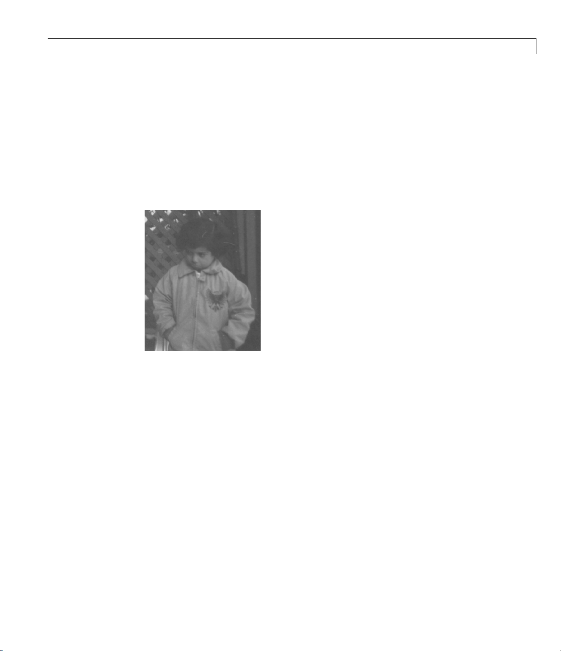
Using an image of an image to corre imagetoidenti characteristi in the image.

fy individual grains. This enables you to learn about the

cs of the grains and easily compute statistics for all the grains

rice grains, this example illustrates how you can enhance

ct for nonuniform illumination, and then use the enhanced

Step 1: Read I

Read and disp

I = imread('rice.png'); imshow(I)

Grayscale Image rice.png

lay the grayscale image

mage

rice.png.

Step 2: Use Morphological Opening to Estimate the Background

In the sample image, the background illumination is brighter in the center of the image than at the bottom. In this step, the example uses a morphological opening operation to estimate the background illumination. Morphological opening is an erosion followed by a d il ation, using the same structuring element for both operations. The opening operation has the effect of removing objects that cannot completely contain the structuring element. For more information about morphological image processing, see Chapter 10, “Morphological Operations”.

1-12

Example 2 — Analyzing Images

background = imopen(I,strel('disk',15));

The example calls the imopen function to perform the morphological opening operation. Note how the example calls the

strel function to create a

disk-shaped structuring element with a radius of 15. To remove the rice grains from the image, the structuring element must be sized so that it cannot fit entirely inside a single grain of rice.

Step 3: View the Background Approximation as a Surface

Use the surf command to create a surface display of the background (the background approximation created in Step 2). The colored parametric surfaces that enable you to view mathematical functions over a rectangular region. However, the

double, so you first need to convert background using the double command:

figure, surf(double(background(1:8:end,1:8:end))),zlim([0 255]); set(gca,'ydir','reverse');

surf function requires data of class

surf command creates

The example uses MATLAB indexing syntax to view only 1 out of 8 pixels in each direction; otherwise, the surface plot would be too dense. The example also sets the scale of the plot to better match the range of the

uint8 data and

reverses the y-axis of the display to provide a b etter view of the data. (The pixels at the bottom of the image appear at the front of the surface plot.)

In the surface display, [0, 0] represents the origin, or upper-left corner of the image. T he highest part of the curve indicates that the highest pixel values of

background (and conseq ue n tly rice.png) occur near the middle rows of

the im age. The lowest pixel values occur at the bottom of the image and are represented in the surface plot by the lowest part of the curve.

The surface plot is a Handle Graphics to fine-tune its appearance. For more information, see the

object. You can use object properties

surface reference

page.

1-13

1 Getting Started

Surface Plot

Step 4: Subtract the Background Image from the Original Image

To create a more uniform background, subtract the background image,

background, from the original image, I, and then view the image:

1-14

I2 = I - background; figure, imshow(I2)

Image with Uniform Background

Example 2 — Analyzing Images

Step 5: Increase

After subtracti dark. Use the contrast of intensities of dynamic range

The following previous ste

I3 = imadjust(I2); figure, imshow(I3);

on, the image has a uniform background but is now a bit too

imadju

I2 and by stretching the intensity values to fill the uint8

example adjusts the contrast in the image created in the

panddisplaysit:

to adjust the contrast of the image. imadjust increases

the image by saturating 1% of the data at both low and high

.Seethe

the Image Contrast

imadjust reference page for more information.

Image After Intensity Adjustment

1-15

1 Getting Started

Step 6: Threshol

Create a binary v the number of ric image into a bin automatically grayscale ima

level = graythresh(I3); bw = im2bw(I3,level); bw = bwareaopen(bw, 50); figure, imshow(bw)

Binary Version of the Image

ersion of the image so you can use toolbox functions to count egrains.Usethe

ary image by using thresholding. The function

computes an appropriate threshold to use to convert the

ge to binary. Remove background noise with

dtheImage

im2bw function to convert the grayscale

graythresh

bwareaopen:

1-16

Step 7: Identify Objects in the Image

The function bwconncomp finds all the connected components (objects) in the binary image. The accuracy of your results depends on the size of the objects, the connectivity parameter (4, 8, or arbitrary), and whether or not any objects are touching (in which case they could be labeled as one object). Some of thericegrainsin

Enter the following at the command line:

cc = bwconncomp(bw, 4) cc.NumObjects

You will receive the output shown below:

bw are touching.

Example 2 — Analyzing Images

cc =

Connectivity: 4

ImageSize: [256 256]

NumObjects: 95

PixelIdxList: {1x95 cell}

ans =

Step 8: Examine One Object

Each distinct object is labeled with the same integer value. Show the grain that is the 50th connected component:

grain = false(size(bw)); grain(cc.PixelIdxList{50}) = true; figure, imshow(grain);

The 50th Connected Component

1-17

1 Getting Started

Step 9: View All O

One way to visual then display it a label matrix fr label matrix in Since

bw conta

labeled = labelmatrix(cc); whos labeled

Name Size Bytes Class Attributes

labeled 256x256 65536 uint8

In the pseud maps to a di to choose t matrix map

RGB_label = label2rgb(labeled, @spring, 'c', 'shuffle'); figure, imshow(RGB_label)

he colormap, the background color, and how objects in the label

ize connected components is to create a label matrix, and

s a pseudo-color indexed image. Use

om the output of

the smallest numeric class necessary for the number of objects.

ins only 95 objects, the label matrix can be stored as

o-color im a ge, the labe l identifying each object in the label matrix

fferent color in the associated colormap matrix. Use

to colors in the colormap:

bjects

labelmatrix to create a

bwconncomp.Notethatlabelmatrix stores the

uint8:

label2rgb

1-18

Label Matrix Displayed as Pseudocolor Image

Example 2 — Analyzing Images

Step 10: Compute Area of Each Object

Each rice grain is one connected component in the cc structure. Use

regionprops on cc to compute the area.

graindata = regionprops(cc, 'basic')

MATLAB responds with

graindata =

95x1 struct array with fields:

Area Centroid BoundingBox

To find the area of the 50th component, use dot notation to access the Area field in the 50th element of graindata structure array:

graindata(50).Area

ans =

194

1-19

1 Getting Started

Step 11: Compute

Create a new vect

grain_areas = [graindata.Area];

Find the grain

[min_area, idx] = min(grain_areas) grain = false(size(bw)); grain(cc.PixelIdxList{idx}) = true; figure, imshow(grain); min_area =

idx =

allgrains to hold the area measurement for each grain:

with the smallest area:

Area-based Statistics

1-20

Smallest Grain

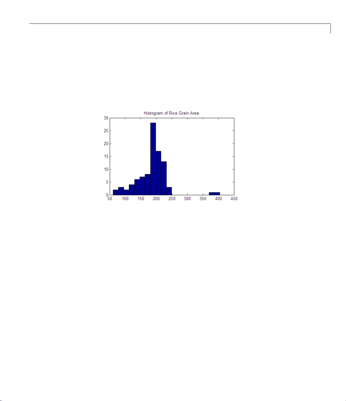
Step 12: Create Histogram of the Area

Use hist to create a histogram of the rice grain area:

nbins = 20; figure, hist(grain_areas, nbins) title('Histogram of Rice Grain Area');

Example 2 — Analyzing Images

1-21

1 Getting Started

Getting Help

In this section...

“Product Documentation” on page 1-22

“Image Processing Demos” on page 1-22

“MATLAB Newsgroup” on page 1-23

Product Documentation

The Image Processing Toolbox documentation is available online in both HTML and PDF formats. To access the HTM L help, select Help from the menu bar of the MATLAB desktop. In the Help Navigator pane, click the Contents tab and expand the Image Processing Toolbox topic in the list.

To access the PDF help, click Image Processing Toolbox in the Contents tab of the Help browser and go to the link under Printable (PDF) Documentation on the Web. (Note that to view the PDF help, you must have

Adobe

Acrobat®Reader installed.)

1-22

For reference information about any of the Image Processing Toolbox functions, see the online Chapter 17, “Functions — Alphabetical List”, which complements the help that is displayed in the MATLAB command window when you type

help functionname

For example,

help imtool

Image Processing Demos

The Image Processing Toolbox software is supported by a full complement of demo applications. These are very useful as templates for your own end-user applications, or for seeing how to use and combine your toolbox functions for powerful image analysis and enhancement.

To view all the demos, call the page in the M ATLAB Help browser that lists all the demos.

iptdemos function. This displays an HTML

Getting Help

You can also view this page by starting the MATLAB Help browser and clicking the Demos icon in the Help Navigator pane.

The toolbox demos are located under the subdirectory

matlabroot\toolbox\images\imdemos

where matlabroot represents your MATLAB installation directory.

MATLAB Newsgroup

If you read newsg roups on the Internet, you might b e interested in the MATLAB newsgroup ( access to an active MATLAB user community. It is an excellent way to seek advice and to share algorithms, sample code, and MATLAB files with other MATLAB users.

comp.soft-sys.matlab). T h is newsgroup gives you

1-23

1 Getting Started

Image Credits

This table lists the copyright owners of the images used in the Image Processing Toolbox documentation.

Image Source

cameraman

cell

Cancer cell from a rat’s prostate, courtesy of Alan W. Partin, M.D., Ph.D., Johns Hopkins University School of Medicine.

circuit

Micrograph of 16-bit A/D converter circuit, courtesy of Steve Decker and Shujaat Nadeem, MIT, 1993.

concordaerial and westconcordaerial

concordorthophoto and westconcordorthophoto

forest

LAN files

liftingbody

m83

oon

saturn

solarspectra

Visible color aerial photographs courtesy of mPower3/Emerge.

Orthoregistered photographs courtesy of Mass achusetts Executive Office of Environmental Affairs, MassGIS.

Photograph of Carmanah Ancient Forest, British Columbia, Canada, courtesy of Susan Cohen.

Permission to use Landsat data sets provided by Space Imaging, LLC, Denver, Colorado.

Picture of M2-F1 lifting body in tow, courtesy of NASA (Image number E-10962).

spiral galaxy astronomical image courtesy

M83

Anglo-Australian Observatory, photography

David Malin.

opyright Michael Myers. Used with

ermission.

oyager 2 image, 1981-08-24, NASA catalog

V #PIA01364.

Courtesy of Ann Walker. Used with permission.

1-24

Image Source

tissue

Courtesy of Alan W. Partin, M.D., PhD., Johns Hopkins University School of Medicine.

trees

Trees with a View, watercolor and ink on paper, copyright Susan Cohen. Used with permission.

Image Credits

1-25

1 Getting Started

1-26

Introduction

This chapter introduces you to the fundamentals of image processing using MATLAB and the Image Processing Toolbox software.

• “Images in MATLAB” on page 2-2

• “Image Coordinate Systems” on page 2-3

• “Image Types in the Toolbox” on page 2-7

• “Converting Between Image Types” on page 2-16

• “Converting Between Image Classes” on page 2-18

• “Working with Image Sequences” on page 2-20

• “Image Arithmetic” on page 2-26

2 Introduction

Images in MATLAB

The basic data structure in MATLAB is the array, an ordered set of real or complex elements. This object is naturally suited to the representation of images, real-valued ordered sets of color or intensity data.

MATLAB stores most images as two-dimensional arrays (i.e., matrices), in which each element of the matrix corresponds to a single pixel in the displayed image. (Pixel is derived from picture element and usually denotes a single dot on a computer display.)

For example, an image composed of 200 rows and 300 columns of different colored dots would be stored in MATLAB as a 200-by-300 matrix. Some images, such as truecolor images, require a three-dimensional array, where thefirstplaneinthethirddimensionrepresents the red pixel intensities, the second plane represents the green pixel intensities, and the third plane represents the blue pixel intensities. This convention makes working with images in MATLAB similar to working with any other type of matrix data, and makes the full power of MATLAB availableforimageprocessingapplications.

2-2

Image Coordinate Systems

In this section...

“Pixel Coordinates” on page 2-3

“Spatial Coordinates” on page 2-4

“Using a Non-Default Spatial Coordinate System” on page 2-5

Pixel Coordinates

Generally, the most convenient method for expressing locations in an image is to use pixel coordinates. In this coordinate system, the image is treated as a grid of discrete elements, ordered from top to bottom and left to right, as illustrated by the fo ll owing figure.

Image Coordinate Systems

The Pixel Coordinate System

For pixel coordinates, the first component r (the row) increases downward, while the second component coordinates are integer values and range between 1 and the length of the row or column.

There is a one-to-one correspondence between pixel coordinates and the coordinatesMATLABusesformatrixsubscripting. T his correspondence makes the relationship between an image’s data matrix and the way the image is displayed easy to understand. For example, the data for the pixel in the fifth row, second column is stored in the matrix element (5,2). You use

c (the column) increases to the right. Pixel

2-3

2 Introduction

normal MATLAB matrix subscripting to access values of individual pixels. For example, the MATLAB code

I(2,15)

returns the value o f the pixel at row 2, column 15 of the image I.

Spatial Coordinates

In the pixel coordinate system, a pixel is treated as a discrete unit, uniquely identified by a single coordinate pair, such as (5,2). From this perspective, a location such as (5.3,2.2) is not meaningful.

At times, however, it is useful to think of a pixel as a square patch. From this perspective, a location such as (5.3,2.2) is meaningful, and is distinct from (5,2). In this spatial coordinate system, locations in an image are positions on a plane, and they are described in terms of the pixel coordinate system).

x and y (not r and c as in

2-4

The following figure illustrates the spatial coordinate system used for images. Notice that

The Spatial Coordinate System

This spatial coordinate system corresponds close ly to the pixel coordinate system in many ways. For example, the spatial coordinates of the center point of any pixel are identical to the pixel coordinates for that pixel.

y increases downward.

Image Coordinate Systems

There are some important d ifferences, however. In pixel coordinates, the upper left corner of an image is (1,1), wh ile in spatial coordinates, this location by default is (0.5,0.5). This difference is due to the pixel coordinate system’s being discrete, while the spatial coordinate system is continuous. Also, the upper left corner is always (1,1) in pixel coordinates, but you can specify a nondefault origin for the spatial coordinate system.

Another potentially confusing difference is largely a matter of convention: the order of the horizontal and vertical components is reversed in the notation for these two systems. As mentioned earlier, pixel co ordinate s are expressed as (

r,c), while spatial coordinates are expressed as (x,y). In the reference pages,

when the syntax for a function uses system. When the syntax uses

r and c, it refers to the pixel coordinate

x and y, it refers to the spatial coordinate

system.

Using a Non-Default Spatial Coordinate System

By default, the spatial coordinates of an image correspond with the pixel coordinates. For example, the center point of the pixel in row 5, column 3 has spatial coordinates is reversed.) This correspondence simplifies many of the toolbox functions considerably. Several functions primarily work with spatial coordinates rather than pixel coordinates, but as long as you are using the default spatial coordinate sy stem, you can specify locations in pixel coordinates.

x=3, y=5. (Remember, the order of the coordinates

In some situations, however, you might want to use a nondefault spatial coordinate sy stem. For example, you could specify that the upper left corner of an image is the point (19.0,7.5), rather than (0.5,0.5). If you call a function that returns coordinates for this image, the coordinates returned will be values in this nondefault spatial coordinate system.

To establish a nondefault spatial coordinate system, you can specify the

XData

and YData image properties when you display the image. These properties are tw o-ele ment vectors that control the range of coordinates spanned by the image. By default, for an image

[1 size(A,1)].

For example, if

[1 200],andthedefaultYData is [1 100]. The values in these vectors are

A is a 100 row by 200 column image, the default XData is

A, XData is [1 size(A,2)],andYData is

actually the coordin a te s for the center points of the first a n d last pixels (not

2-5

2 Introduction

the pixel edges), so the actual coordinate range spanned is slightly larger; for instance, if

[0.5 200.5].

XData is [1 200],thex-axis range spanned by the image is

These commands display an image using nondefault

A = magic(5); x = [19.5 23.5]; y = [8.0 12.0]; image(A,'XData',x,'YData',y), axis image, colormap(jet(25))

XData and YData.

2-6

For information about the syntax variations that specify nondefault spatial coordinates, see the reference page for

imshow.

ImageTypesintheToolbox

In this section...

“Overview of Image Types” on page 2-7

“Binary Images” on pa ge 2-8

“Indexed Images” o n page 2-9

“Grayscale Images” on page 2-11

“Truecolor Images” on page 2-12

Overview of Image Types

The Image Processing Toolbox software defines four basic types of images, summarized in the following table. These image types determine the way MATLAB interprets data matrix elements as pixel intensity values. For information about converting between image types, see “Converting Between Image Types” on page 2-16.

ImageTypesintheToolbox

Image Ty

Binary (Also known as a bilevel image)

Indexed (Also known as a pseudocolor im age)

Interpr

Logical array containing only 0s a nd 1s, interpreted

as black and white, respectively. See “Binary Images” on page 2-8 for more information.

Array of class

double whose pixel values are direct indices into a

colormap. The colormap is an m-by-3 array of class

double.

For from [1, p]. For values range from [0, p-1]. See “Indexed Images” on page 2-9 for more information.

etation

logical, uint8, uint16, single,or

single or double arrays, integer values range

logical, uint8,oruint16 arrays,

2-7

2 Introduction

Image Type Interpretation

Grayscale (Also known as an intensity, gray scale, or gray level image)

Array of class

double w hose pixel v alues specify intensity values.

single or double arrays, values range from

For [0, 1]. For

uint16, values range from [0, 65535]. For int16,

uint8, uint16, int16, single,or

uint8, values range from [0,255]. For

values range from [-32768, 32767]. See “Grayscale Images” on page 2-11 for more information.

Truecolor (Also known as an

RGB image )

m-by-n-by-3 array of class

double w hose pixel v alues specify intensity values.

single or double arrays, values range from

For [0, 1]. For

uint8, values range from [0, 255]. For

uint8, uint16, single,or

uint16, values range from [0, 65535]. See “Truecolor Images” on page 2-12 for more information.

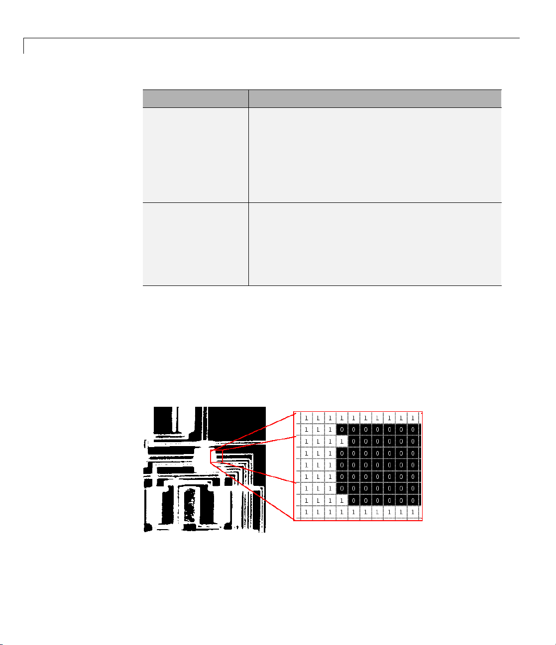
Binary Images

In a b i na ry image, each pixel assumes one of only two discrete values: 1 or 0. A binary image is stored as a documentation uses the variable name

The following figure shows a binary image with a close-up view of some of the pixel values.

logical array. By convention, this

BW to refer to binary images.

2-8

Pixel Values in a Binary Image

Indexed Images

An indexed image values in the arr documentation to the colormap

The colormap m floating-poi

nt values in the range [0,1]. Each row of green, and bl mapping of pi determined b

consists of an array and a colormap matrix. The pixel

ay are direct indices into a colormap. By convention, this

uses the variable name

atrix

ue components of a single color. An indexed image uses direct

xel values to colormap values. The color of each image pixel is

y using the corresponding value of

ImageTypesintheToolbox

X to refer to the array and map to refer

isanm-by-3 array of class double containing

map specifies the red,

X as an index into map.

2-9

2 Introduction

A colormap is often stored with an indexed image and is automatically loaded with the image when you use the

imread function. After you read the

image and the colormap into the MATLAB workspace as separate variables, you must keep track of the association between the image and colormap. However, you are not lim ited to using the default colormap--you can use any colormap that you choose.

The relationship between the values in the image matrix and the colormap depends on the class of the image matrix. If the image matrix is of class

single or double, it normally contains integer values 1 through p,wherep is

the length of the colormap. the value 1 points to the first row in the colormap, the value 2 points to the second row, and so on. If the image matrix is of class

logical, uint8 or uint16, the value 0 points to the first row in the colormap,

the value 1 points to the second row, and so on.

The following figure illustrates the structure of an indexed image. In the figure, the image matrix is of class

double,sothevalue5pointstothefifth

row of the colormap.

2-10

el Values Index to Colormap Entries in Indexed Images

Pix

ImageTypesintheToolbox

Grayscale Image

A grayscale imag matrix whose val stores a graysc matrix corresp uses the varia

The matrix can grayscale im to display th

For a matrix the intensi matrix of ty represent

The figure

ty 0 represents black and the intensity 1 represents white. For a

s black and the intensity

e (also called gray-scale, gray scale, or gray-level) is a data

ues represent intensities within some range. MATLAB ale image as a individual matrix, with each element of the onding to one image pixel. By convention, this documentation

ble name

be of class

ages are rarely saved with a colormap, MATLAB uses a colormap

em.

of class

below d epicts a grayscale image of class

single or double, using the d efault grayscale colormap,

uint8, uint16,orint16, the inten s ity intmin(class(I))

I to refer to grayscale images.

uint8, uint16, int16, single,ordouble.While

intmax(class(I)) represents white.

double.

Pixel Values in a Grayscale Image Define Gray Levels

2-11

2 Introduction

Truecolor Image

A truecolor imag —oneeachforthe MATLAB store tr red, green, and images do not u combination o at the pixel’s

Graphics fil green, and bl million col has led to th

A truecolo truecolor between 0 a as black, white. Th dimensio compone

RGB(10,

r array can be of class

array of class

and a pixel whose color components are (1,1,1) is displayed as

e three color components for each pixel are stored alo ng the third

n of the data array. For example, the red, green, and blue color

nts of the pixel (10,5) are stored in

5,3)

e is an image in which each pixel is specified by three values

red, blue, and green components of the pixel’s color.

uecolorimagesasanm-by-n-by-3 data array that defines

blue color compo n en ts for each individual pixel. Truecolor

se a colormap. The color of each pixel is determined by the

f the red, green, and blue intensities stored i n each color plane

location.

e formats store truecolor images as 24-bit images, where the red,

ue components are 8 bits each. This yields a potential of 16

ors. The precision with which a real-lifeimagecanbereplicated

e commonly used term truecolor image.

nd 1. A pixel whose color com po nents are ( 0, 0,0) is disp layed

,respectively.

uint8, uint16, single,ordouble.Ina

single or double, each color component is a value

RGB(10,5,1), RGB(10,5,2),and

2-12

The following figure depicts a truecolor image of class double.

ImageTypesintheToolbox

The Color Planes of a Truecolor Image

To determine the color of the pixel at (2,3), you would look at the RGB triplet stored in (2,3,1:3). Suppose (2,3,1) contains the value

0.1608, and (2,3,3) contains 0.0627.Thecolorforthepixelat(2,3)is

0.5176 0.1608 0.0627

0.5176, (2,3,2) contains

2-13

2 Introduction

To further illustrate the concept of the three separate color planes used in a truecolor image, the code sample below creates a simple image containing uninterrupted areas of red, green, and blue, and then creates one image for each of its separate color planes (red, green, and blue). The example displays each color plane image separately, and also displays the original image.

RGB=reshape(ones(64,1)*reshape(jet(64),1,192),[64,64,3]); R=RGB(:,:,1); G=RGB(:,:,2); B=RGB(:,:,3); imshow(R) figure, imshow(G) figure, imshow(B) figure, imshow(RGB)

2-14

The Separated Color Planes of an RGB Image

ImageTypesintheToolbox

Notice that each separated color plane in the figure contains an area of white. The w hite corresponds to the h ighest values (purest shades) of each separate color. For example, in the Red Plane image, the white represents the highest concentration of pure red values. As red becomes mixed with green or blue, gray pixels appear. The black region in the image shows pixel values that contain no red values, i.e.,

R==0.

2-15

2 Introduction

Converting Between Image Types

The toolbox includes many functions that y ou can use to convert an image from one type to another, listed in the following table. For example, if you want to filter a color image that is stored as an indexed image, you must first convert it to truecolor format. When you apply the filter to the truecolor image, MATLAB filters the intensity values in the image, as is appropriate. If you attempt to filter the indexed image, MATLAB simply applies the filter to the indices in the indexed image matrix, and the results might not be meaningful.

You can perform certain conversions just using MATLAB syntax. For example, you can convert a grayscale image to truecolor format by concatenating three copies of the original m atrix along the third dimension.

RGB = cat(3,I,I,I);

The resulting truecolor image has identical matrices for the red, green, and blueplanes,sotheimagedisplaysasshadesofgray.

2-16

In addition to these image type conversion functions, there are other functions that return a different image type as part of the operation they perform. For example, the region of interest functions return a binary image that you can use to mask an image for filtering or for other operations.

Note When you convert an image from one format to another, the resulting image might look different from the original. For example, if you convert a color indexed image to a grayscale image, the resulting image displays as shades of grays, not color.

ion

Funct

saic

demo

her

dit

gray2ind

iption

Descr

ert Bayer pattern encoded image to truecolor (RGB)

Conv

imag

Use dithering to convert a grayscale image to a binary image or to convert a truecolor image to an indexed image.

Convert a grayscale image to an indexed image.

Function Description

grayslice

Convert a grayscale image to an indexed ima g e by using multilevel thresholding.

im2bw

Convert a grayscale image, indexed image, or truecolor image, to a binary image, based on a luminance threshold.

ind2gray

ind2rgb

mat2gray

Convert an indexed image to a grayscale image.

Convert a n indexed image to a truecolor image.

Convert a data matrix to a grayscale image, by scaling the data.

rgb2gray

Convert a truecolor image to a grayscale image.

Note: To work with images that use o the r color spaces, such as HSV, first convert the image to RGB, process the image, and then convert it back to the original color space. For more information about color space conversion routines, see Chapter 14, “Color”.

rgb2ind

Convert a truecolor image to an indexed image.

Converting Between Image Types

2-17

2 Introduction

Converting Between Image Classes

In this section...

“Overview of Image Class Conversions” on page 2-18

“Losing Information in Conversions” on page 2-18

“Converting Indexed Images” on page 2-18

Overview of Image Class Conversions

You can convert uint8 and uint16 image data to double using the MATLAB

double function. However, converting between classes changes the way

MATLAB and the toolbox interpret the image data. If you want the resulting array to be interpreted properly as image data, you need to rescale or offset the data when you convert it.

For easier conversion of classes, use one of these functions:

im2uint16, im2int16, im2single,orim2double.Thesefunctions

automatically handle the rescaling and offsetting of the original data of any image class. For example, this command converts a double-precision RGB image with data in the range [0,1] to a range [0,255].

RGB2 = im2uint8(RGB1);

uint8 RGB image with data in the

im2uint8,

Losing Information in Conversions

When you convert to a class that uses fewer bits to represent numbers, you generally lose some of the information in your image. For example, a grayscale image is capable of storing up to 65,536 distinct shades of gray, but a

uint8 grayscale image can store only 256 distinct shades of gray. W hen

you convert a quantizes the gray shades in the original image. In other words, all values from 0 to 127 in the original image become 0 in the 128 to 385 all become 1, and so on.

uint16 grayscale image to a uint8 grayscale image, im2uint8

uint8 image, values from

uint16

Converting Indexed Images

It is not always possible to convert an indexed image from one storage class to another. In an indexed image, the image matrix contains only indices into

2-18

Converting Between Image Classes

a colormap, rather than the color data itself, so no quantization of the color data is possib le during the conversion.

For example, a converted to

uint16 or double indexed image with 300 colors cannot be

uint8,becauseuint8 arrays have only 256 distinct values. If

you want to perform this conversion, you must first reduce the number of the colors in the image using the

imapprox function. This function performs the

quantization on the colors in the colormap, to reduce the number of distinct colors in the image. See “Reducing Colors Using imapprox” on page 14-10 for more information.

2-19

2 Introduction

Working with Image Sequences

In this section...

“Overview of Toolbox Functions That Work with Image Sequences” on page 2-20

“Example: Processing Image Sequences” on page 2-23

“Multi-Frame Image Arrays” on page 2-24

Overview of Toolbox Functions That Work with Image Sequences

Some applications work with collections of images related by time, such as frames in a movie, or by (spatial location, such as magnetic resonance imaging (MRI) slices. These colle ctions of images are referred to by a variety of names, such as image sequences or image stacks.

The ability to create N-dimensional arrays can provide a convenient way to store image sequences. For example, an m-by-n-by-p array can store an array of p two-dimensional images, such as grayscale or binary images, as shown in the following figure. A n m-by-n-by-3-by-p array can store truecolor images where each image is made up of three planes.

2-20

tidimensional Array Containing an Image Sequence

Mul

y toolbox functions can operate on m ulti-dimensional arrays and,

Man

nsequently, can operate on image sequences. For example, if you pass a

lti-dimensional array to the

ansformation to all 2-D planes along the higher dimension.

imtransform function, it applies the same 2-D

Working with Image Sequences

Some toolbox functions that accept multi-dimensional arrays, however, do not by default interpret an m-by-n-by-p or an m-by-n-by-3-by-p array as an image sequence. To use these functions with image sequences, you must use particular syntax and be aware of other limitations. The following table lists these toolbox functions and provides guidelines about how to use them to process image sequences. For information about displaying image sequences, see “Viewing Image Sequences” on page 4-55.

Function

bwlabeln

deconvblind

deconvlucy

edgetaper

entropyfilt

imabsdiff

imadd

imbothat

imclose

imdilate

imdivide

imerode

imextendedmax

Image Sequence Dimensions

Guideline When Used with an Image Sequence

m-by-n-by-p only Must use the bwlabeln(BW,conn)

syntax with a 2-D connectivity.

m-by-n-by-p or m-by-n-by-3-by-p

PSF argument can be either 1-D

or 2-D.

PSF argument can be either 1-D

or 2-D.

PSF argument can be either 1-D

or 2-D.

m-by-n-by-p only nhood argument must be 2-D. m-by-n-by-p or

m-by-n-by-3-by-p m-by-n-by-p or

m-by-n-by-3-by-p

Image sequences must be the same size.

Image sequences must be the same size. Cannot add scalar to image sequence.

m-by-n-by-p only SE argument must be 2-D. m-by-n-by-p only SE argument must be 2-D. m-by-n-by-p only SE argument must be 2-D. m-by-n-by-p or

m-by-n-by-3-by-p

Image sequences must be the same size.

m-by-n-by-p only SE argument must be 2-D. m-by-n-by-p only Must use the

imextendedmax(I,h,conn)

syntax with a 2-D connectivity.

2-21

2 Introduction

Function

imextendedmin

imfilter

imhmax

imhmin

imlincomb

immultiply

imopen

imregionalmax

imregionalmin

imtransform

imsubtract

imtophat

padarray

rangefilt

stdfilt

Image Sequence Dimensions

Guideline When Used with an Image Sequence

m-by-n-by-p only Must use the

imextendedmin(I,h,conn)

syntax with a 2-D connectivity.

m-by-n-by-p or m-by-n-by-3-by-p

With grayscale images, h can be 2-D. With truecolor images (RGB),

h can be 2-D or 3-D.

m-by-n-by-p only Must use the imhmax(I,h,conn)

syntax with a 2-D connectivity.

m-by-n-by-p only Must use the imhmin(I,h,conn)

syntax with a 2-D connectivity.

m-by-n-by-p or m-by-n-by-3-by-p

Image sequences must be the same size.

m-by-n-by-p only SE argument must be 2-D. m-by-n-by-p only Must use the

imextendedmax(I,conn) syntax

with a 2-D connectivity.

m-by-n-by-p only Must use the

imextendedmin(I,conn) syntax

with a 2-D connectivity.

m-by-n-by-p or

TFORM argument must be 2-D.

m-by-n-by-3-by-p m-by-n-by-p or

m-by-n-by-3-by-p

Image sequences must be the same size.

m-by-n-by-p only SE argument must be 2-D. m-by-n-by-p or

m-by-n-by-3-by-p

PADSIZE argument must be a

two-element vector.

m-by-n-by-p only NHOOD argument must be 2-D. m-by-n-by-p only NHOOD argument must be 2-D.

2-22

Working with Image Sequences

Function

tformarray

Image Sequence Dimensions

m-by-n-by-p or m-by-n-by-3-by-p

Guideline When Used with an Image Sequence

T must be 2-D to 2-D (compatible

with

imtransform). R must be 2-D. TDIMS_A and TDIMS_B must be 2-D,

i.e.,

[2 1] or

[

12]

TSIZE_B

array

must be a two-element

[D1 D2],whereD1 and D2

are the first and second transform dimensions of the output space.

TMAP_B must be [TSIZE_B 2]

can be a scalar or a p-by-1

array for m-by-n-by-p arrays, or it can be a scalar, 1-by-p array, 3-by-1 array, or 3-by-p array, for m-by-n-by-3-by-p arrays.

watershed

m-by-n-by-p only

Must use

watershed(I,conn)

syntax with a 2-D connectivity.

Example: Processing Image Sequences

This example starts by reading a series of images from a directory into the MATLAB workspace, storing the images in an m-by-n-by-p array. The example then passes the entire array to the standard deviation filtering on each image in the sequence. Note that, to use

stdfilt with an image sequence, you must use the nhood argument,

specifying a 2-D neighborhood.

stdfilt function and performs

% Create an array of filenames that make up the image sequence fileFolder = fullfile(matlabroot,'toolbox','images','imdemos'); dirOutput = dir(fullfile(fileFolder,'AT3_1m4_*.tif')); fileNames = {dirOutput.name}'; numFrames = numel(fileNames);

I = imread(fileNames{1});

% Preallocate the array

2-23

2 Introduction

sequence = zeros([size(I) numFrames],class(I)); sequence(:,:,1) = I;

% Create image sequence array for p = 2:numFrames

sequence(:,:,p) = imread(fileNames{p});

end

% Process sequence sequenceNew = stdfilt(sequence,ones(3));

% View results figure; for k = 1:numFrames

imshow(sequence(:,:,k)); title(sprintf('Original Image # %d',k)); pause(1); imshow(sequenceNew(:,:,k),[]); title(sprintf('Processed Image # %d',k)); pause(1);

end

2-24

Multi-Frame Image Arrays

The toolbox includes two functions, immovie and montage,thatworkwitha specific type o f multi-dimensiona l array called a multi-frame array. In this array, images, called frames in this context, are concatenated along the fourth dimension. Multi-frame arrays are either m-by-n-by-1-by-p, for grayscale, binary, or indexed images, or m-by-n-by-3-by-p, for truecolor images, where p is the number of frames.

For example, a multi-frame array containing five, 480-by-640 grayscale or indexed images would be 480-by-640-by-1-by-5. An array with five 480-by-640 truecolor images would be 480-by-640-by-3-by-5.

Note To process a multi-frame array of grayscale images as an image sequence, as described in “Working with Image Sequences” on page 2-20, you can use the

squeeze function to remove the singleton dimension.

Working with Image Sequences

You can use the cat command to create a multi-frame a rray. For example, the following stores a group of images (

A = cat(4,A1,A2,A3,A4,A5)

A1, A2, A3, A4,andA5) in a single array.

You can also extract frames from a multiframe image. For example, if you have a multiframe image

FRM3 = MULTI(:,:,:,3)

MULTI, this command extracts the third frame.

Note that, in a multiframe image array, each image must be the same size and have the same number of planes. In a multiframe indexed image, each imagemustalsousethesamecolormap.

2-25

2 Introduction

Image Arithmetic

In this section...

“Overview o f Image Arithmetic Functions” on page 2-26

“Image Arithmetic Saturation Rules” on page 2-27

“Nesting Calls to Image Arithmetic Functions” on page 2-27

Overview of Image Arithmetic Functions

Image arithmetic is the implementation of standard arithmetic operations, such as addition, subtraction, multiplication, and division, on images. Image arithmetic has many uses in image processing both as a preliminary step in more complex operations and by itself. For example, image subtraction can be use d to detect differences between two or more images of the same scene or object.

You can do image arithmetic using the MAT LAB arithmetic operators. The Image Processing Toolbox software also includes a set of functions that implement arithmetic operations for all numeric, nonsparse data types. The toolbox arithmetic functions accept any numeric data type, including same format. The functions perform the operations in double precision, on an element-by-element basis, but do not convert images to double-precision values in the MATLAB w orkspace . Ov erflow is handled automatically. The functions saturate return values to fit the data type. For more information, see these additional topics:

uint8, uint16,anddouble, and return the result image in the

2-26

Note On Intel®architecture processors, the image arithmetic functions can take advantage of the Intel Integrated Performance Primitives (Intel IPP) library, thus accelerating their execution time. The Intel IPP library is only activated, however, when the data passed to these functions is of specific classes. See the reference pages for the individual arithmetic functions for more information.

Image Arithmetic

Image Arithmeti

The results of in for storage. For

255. Arithmeti be represented

MATLAB arithm functions use

• Values that e

• Fractional

For example

Inf)areset

Result Class Truncated Value

300

-45

10.5

Nestin

You ca of ope

g Calls to Image Arithmetic Functions

n use the image arithmetic functions in combination to perform a series

rations. For example, to calculate the average of two images,

teger arithmetic can easily overflow the data type allotted example, the maximum value you can store in

c operations can also result in fractional values, which cannot

using integer arrays.

etic operators and the Image Processing Toolbox arithmetic

these rules for integer arithmetic:

xceed the range of the integer type are saturated to that range.

values are rounded.

,ifthedatatypeis

to 255. The following table lists some additional exam ples.

cSaturationRules

uint8, results greater than 255 (including

uint8

uint8 11

uint8 data is

255

ould enter

You c

I = imread('rice.png'); I2 = imread('cameraman.tif'); K = imdivide(imadd(I,I2), 2); % not recommended

en used with

d saturates its result before passing it on to the next operation. This can

ignificantly reduce the precision of the calculation. A better w ay to perform

uint8 or uint16 data, each arithmetic function rounds

2-27

2 Introduction

this ca lcu latio n is to use th e imlincomb function. imlincomb perfo r ms all the arithmetic operations in the linear combination in double precision and only rounds and saturates the final result.

K = imlincomb(.5,I,.5,I2); % recommended

2-28

Reading and Writing Image Data

This chapter describes how to get inform ation about the contents of a graphics file, read image data from a file, and write image data to a file, using standard graphics and medical file formats.

• “Getting Information About a Graphics File” on page 3-2

• “Reading Image Data” on page 3-3

• “WritingImageDatatoaFile”onpage3-5

• “Converting Between Graphics File Formats” on page 3-8

• “Working with DICOM Files” on page 3-9

• “Working with Mayo Analyze 7.5 Files” on page 3-19

• “Working with Interfile Files” on page 3-20

• “Working with High Dynamic Range Images” on page 3-21

3 Reading and Writing Image Data

Getting Information About a Graphics File

To obtain information about a graphics file and its contents, use the imfinfo function. You can use imfinfo with any of the formats supported by MATLAB. Use the

Note Y ou can also get information about an image displayed in the Image Tool — see “Getting Information About an Image Using the Image Information Tool” on page 4-40 .

The information returned by imfinfo depends on the file format, but it always includes at least the following:

• Name of the file

• File format

• Version number of the file format

imformats function to determine which formats are supported.

3-2

• File modification date

• File size in bytes

• Image width in pixels

• Image height in pixels

• Number of bits per pixel

• Image type: truecolor (RGB), grayscale (intensity), or indexed

Reading Image Data

To import an image from any supported graphicsimagefileformat,inany of the supported bit depths, use the truecolor image into the MATLAB workspace as the variable

RGB = imread('football.jpg');

If the image file format uses 8-bit pixels, imread stores the data in the workspace as a PNG and TIFF,

imread uses two variables to store an indexed image i n the workspace: one

for the image and another for its associated colormap. thecolormapintoamatrixofclass itself may be of class

[X,map] = imread('trees.tif');

Reading Image Data

imread function. Thisexamplereadsa

RGB.

uint8 array. For file formats that support 16-bit data, such as

imread creates a uint16 array.

imread always reads

double,eventhoughtheimagearray

uint8 or uint16.

In these examples, imread infersthefileformattousefromthecontentsofthe file. You can also specify the file format as an argument to supports many common graphics file formats, such as Microsoft®Windows

imread. imread

Bitmap (BMP), Graphics Interchange Format (GIF), Joint Photographic Experts Group (JPEG), Portable Network Graphics (PNG), and Tagged Image File Format (TIFF) formats. For the latest information concerning the bit depths and/or image formats supported, see

If the graphics file contains multiple images, image from the file. To import additional images, you must use

imread and imformats.

imread imports only the first

imread with

format-specific arguments to specify the image you want to import. In this example, images in a four-dimensional array. You can use

imread imports a series of 27 images from a T IFF file and stores the

imfinfo to determine how

many images are stored in the file.

mri = zeros([128 128 1 27],'uint8'); % preallocate 4-D array

for frame=1:27

[mri(:,:,:,frame),map] = imread('mri.tif',frame);

end

3-3

3 Reading and Writing Image Data

When a file contains multiple images that are related in some way, you can call image processing algo rithms directly. . For more information, see “Working with Image Sequences” on page 2-20.

3-4

Writing Image Data to a File

In this section...

“Overview” on page 3-5

“Specifying Format-Specific Param eters” on page 3-6

“Reading and Writing Binary Images in 1-Bit Format” on page 3-6

“Determining the Storage Class of the Output File” on page 3-7

Overview

To export image data from the MATLAB workspace to a graphics file in one of the supported graphics file formats, use the

imwrite, you specify the MATLAB variable name and the name of the file.

If you include an extension in the filename, desired file format from it. For example, the file extension Joint Photographic Experts Group (JPEG) format. You can also specify the format explicitly as an argument to

Writing Image Data to a File

imwrite function. When using

imwrite attempts to infer the

.jpg infers the

imwrite.

This example loads the indexed image with the associated colormap

map, and then exports the image as a bitmap

X from a MAT-file, clown.mat,along

(BMP) file.

load clown whos

Name Size Bytes Class

X 200x320 512000 double array caption 2x1 4 char array map 81x3 1944 double array

Grand total is 64245 elements using 513948 bytes

imwrite(X,map,'clown.bmp')

3-5

3 Reading and Writing Image Data

Specifying Format-Specific Parameters

When using imwrite with some graphics formats, you can specify additional format-specific parameters. For example, with PNG files, you can specify the bit depth. This example writes a grayscale image

imwrite(I,'clown.png','BitDepth',4);

This example writes an image A to a JPEG file, using an additional parameter to specify the compression quality parameter.

imwrite(A, 'myfile.jpg', 'Quality', 100);

For more information about these additional format-specific syntaxes, see the

imwrite reference page.

Reading and Writing Binary Images in 1-Bit Format

In certain file form ats, such as TIFF, a binary image can be stored in a 1-bit format. W hen you read in a binary image in 1-bit format, data in the workspace as a

imwrite writes binary images as 1-bit images by default. This example reads

in a binary image and writes it as a TIFF file.

I to a 4-bit PNG file.

imread stores the

logical array. If the file format supports it,

3-6

BW = imread('text.png'); imwrite(BW,'test.tif');

To verify the bit depth of test.tif,callimfinfo and check the BitDepth field.

info = imfinfo('test.tif');

info.BitDepth ans =

Note When writing binary files, MATLAB sets the ColorType field to

'grayscale'.

Writing Image Data to a File

Determining the Storage Class of the Output File

imwrite uses the following rules to determine the storage class used in the

output image.

Storage Class of Image Storage Class of Output Image File

logical

uint8

uint16

int16

single

double

If the output image file form at supports 1-bit images,

imwrite creates a 1-bit image file.

If the output image file format specified does not support 1-bit images, as a

uint8 grayscale image.

imwrite exports the image data

If the output image file format supports unsigned 8-bit images,

imwrite creates an unsigned 8-bit image file.

If the output image file format supports unsigned 16-bit images (PNG or TIFF),

imwrite creates an unsigned

16-bit image file.

If the output image file format does not support 16-bit images,

imwrite scales the image data to class uint8

and creates an 8-bit image file.

Partially supported; depends on file format.

MATLAB scales the image data to uint8 and creates an 8-bit image file, because most image file formats use 8bits.

3-7

3 Reading and Writing Image Data

Converting Between Graphics File F ormats

To change the graphics format of an image, use imread to import the image into the MATLAB workspace and then use the image, specifying the appropriate file format.

imwrite function to export the

To illustrate, this example uses the format into the workspace and write the image data as JPEG format.

moon_tiff = imread('moon.tif'); imwrite(moon_tiff,'moon.jpg');

For the specifics of which bit depths are supported for the different graphics formats,andforhowtospecifytheformattypewhenwritinganimagetofile, see the reference pages for

imread and imwrite.

imread function to read an image in TIFF

3-8

Working with DICOM Files

In this section...

“Overview of DICOM Support” on page 3-9

“Reading Metadata from a DICOM File” on page 3-10

“Reading Image Data from a DICOM File” on page 3-12

“Writing Image Data or Metadata to a DICOM File” on page 3-13

Overview of DICOM Support

The D igital Imaging and Communications in Medicine (DICOM) Standard is a joint project of the American College of R a diology (ACR) and the National Electrical Manufacturers Association (NEMA ). The standard facilitates interoperability of medical imaging equipment by specifying a set of media storage services , a file format, and a medical directory structure to facilitate access to the images and related information stored on interchange media. For detailed information about the standard, see the official DICOM web site.

Working with DICOM Files

The MathWorks provides the following support for working with files in the DICOM format:

• Reading any file that complies with the DICOM standard

• Writing three different types of DICOM files, or DICOM information

objects (IOD), with validation:

- Secondary capture (default)

- Magnetic resonance

- Computed tomography

• Writing many more types of DICOM files without validation, b y setting the

createmode flag to 'copy' when writing data to a file.

Note MATLAB supports working with DICOM files. There is no support for working with DICOM network capabilities.

3-9

3 Reading and Writing Image Data

Reading Metadata from a DICOM File

DICOM files contain metadata that provide information about the image data, such as the size, dimensions, bit depth, modality used to create the data, and equipment settings used to capture the image. To read metadata from a DICOM file, use the in a MATLAB structure where every field contains a specific piece o f DICOM metadata. You can use the metadata structure returned by specify the DICOM file you want to read using Image Data from a DICOM File” on page 3-12.

The following example reads the metadata from a sample DICOM file that is included with the toolbox.

info = dicominfo('CT-MONO2-16-ankle.dcm')

info =

dicominfo function. dicominfo returns the information

dicominfo to

dicomread — see “Reading

Filename: [1x47 char]

FileModDate: '24-Dec-2000 19:54:47'

FileSize: 525436

Format: 'DICOM'

FormatVersion: 3

Width: 512

Height: 512

BitDepth: 16

ColorType: 'grayscale'

SelectedFrames: []

FileStruct: [1x1 struct]

StartOfPixelData: 1140

MetaElementGroupLength: 192

FileMetaInformationVersion: [2x1 double]

MediaStorageSOPClassUID: '1.2.840.10008.5.1.4.1.1.7'

MediaStorageSOPInstanceUID: [1x50 char]

TransferSyntaxUID: '1.2.840.10008.1.2'

ImplementationClassUID: '1.2.840.113619.6.5'

. . .

3-10

Working with DICOM Files

Handling Private Metadata

The DICOM specification defines many of these metadata fields, but files can contain additional fields, called private metadata. This private metadata is typically defined by equipment vendors to provide additional information about the data they provide.

When

dicominfo encounters a private metadata field in a DICOM file, it

returns the metadata creating a genericnameforthefieldbasedonthe group and element tags of the metadata. For example, if the file contained private metadata at group 0009 and element 0006, name:

Private_0009_0006. dicominfo attempts to interpret the private

metadata, if it can. For example, if the metadata is a text string,

dicominfo creates the

dicominfo

processes the data. If it can’t interpret the data, dicominfo returns a sequence of bytes.

If you need to process a DICOM file created by a manufacturer that uses private metadata, and you prefer to view the correct name of the field as well as the data, you can create your own copy of the DICOM data dictionary and update it to include definitions of the private metadata. You will need information about the private metadata th at vendors typically provide in DICOM compliance statements. For more information about updating DICOM dictionary, see “Creating Your Own Copy of the DICOM Dictionary” on page 3-11.

Creating Your Own Copy of the DICOM Dictionary

The MathWorks uses a DICOM dictionary that contains definitions of thousands of standard DICOM metadata fields. If your DICOM file contains metadata that is not defined this dictionary, you can update the dictio na ry, creating your own copy that it includes these private m etadata fields.

To create your own dictionary, perform this procedure:

1 Make a copy of the text version of the DICOM dictionary that

is included with MATLAB. This file, called

dicom-dict.txt

is located in matlabroot/toolbox/images/medformats or

matlabroot/toolbox/images/iptformatsdepe n ding on which version

of the Image Processing Toolbox software you are working with. Do not attempt to edit the MAT-file version of the dictionary,

dicom-dict.mat.

3-11

3 Reading and Writing Image Data

2 Edit your copy of the DICOM dictionary, adding entries for the metadata.

Insert the new metadata field using the group and element tag, type, and other information. Follow the format of the other entries in the file. The creator of the metadata (e.g., an equipment vendor) must provide you with the information.

3 Save your copy of the dictionary.

4 Set MATLAB to use your copy of the DICOM dictionary, dicomdict

function.

Reading Image Data from a DICOM File

To read image data from a DICOM file, use the dicomread function. The

dicomread function reads files that comply with the DICOM specification but

can also read certain common noncomplying files.

When using

dicomread, you can specify the filename as an argument, as

in the following example. The example reads the sampl e DICOM file that is included with the toolbox.

I = dicomread('CT-MONO2-16-ankle.dcm');

You can also use the metadata structure returned by dicominfo to specify the file you want to read, as in the following example.

info = dicominfo('CT-MONO2-16-ankle.dcm'); I = dicomread(info);

Viewing Images from DICOM Files

To view the image data imported from a DICOM file, use one of the toolbox image display functions the image data in this DICOM file is signed 16-bit data, you must use the autoscaling syntax with either display function to make the image viewable.

imshow(I,'DisplayRange',[])

imshow or imtool. Note, however, that because

3-12

Working with DICOM Files

Writing Image Data or Metadata to a DICOM File

To write image data or metadata to a file in DICOM format, use the

dicomwrite function. This e xample writes the image I to the DICOM file ankle.dcm.

dicomwrite(I,'ankle.dcm')

Writing

Metadata with the Image Data

When writing image data to a DICOM file, dicomwrite automatically includes the minimum set of metadata fields required by the type of DICOM information object (IOD) you are creating.

dicomwrite supports the following

DICOM IODs with full validation.

• Secondary capture (default)

• Magnetic resonance

• Computed tomography

dicomwrite can write many other types of DICOM data (e.g. X-ray,

radiotherapy, nuclear medicine) to a file; however, perform any validation of this data. See

dicomwrite for more information.

dicomwrite does not

3-13

3 Reading and Writing Image Data

You can also specify the metadata you want to write to the file by passing to

dicomwrite an existing DICOM metadata structure that you retrieved using dicominfo. In the following example, the dicomwrite function writes the

relevant information in the metadata structure

info = dicominfo('CT-MONO2-16-ankle.dcm'); I = dicomread(info); dicomwrite(I,'ankle.dcm',info)

Note that the metadata written to the file is not identical to the metadata in the

info structure. When writing metadata to a file, there are certain fields

that

dicomwrite must update. To illustrate, look at the instance ID in the

original metadata with the ID in the new file.

info.SOPInstanceUID ans =

1.2.840.113619.2.1.2411.1031152382.365.1.736169244

info to the new DICOM file.

3-14

Now, read the metadata from the newly created DICOM file, using dicominfo, and check the

info2 = dicominfo('ankle.dcm');

info2.SOPInstanceUID

ans =

1.2.841.113411.2.1.2411.10311244477.365.1.63874544

SOPInstanceUID field. Note that they contain different values.

Understanding Explicit Versus Implicit VR Attributes

DICOM attributes provide the length and then the data. When writing data to a file, you can include a two-letter value representation (VR) with the attribute or you can let DICOM infer the value representation from the d ata dictionary. When you specify the VR option with the value the

dicomwrite function includes the VR in the attribute. The following figure

shows the attributes with and without the VR.

'explicit' ,

Working with DICOM Files

Removing Confidential Information from a DICOM File

When using a DICOM file as part of a training set, blinded study, or a presentation, you might want to remove confidential patient information, a process called anonymizing the file. To do this, use the

The

dicomanon function creates a new series with new study values, changes

dicomanon function.

some of the metadata, and then writes the file. For example, you could replace steps 4, 5, and 6 in the example i n “Example: Creating a New DICOM Series” on page 3-15 with a call to the

dicomanon function.

Example: Creating a New DICOM Series

When writing a modified image to a DICOM file, you might want to make the modified image the start of a new series. In the DICOM standard, images can be organized into series. When you write an image with metadata to a DICOM file, create a new series, you must assign a new DICOM unique identifier to the

SeriesInstanceUID metadata field. The following example illustrates this

process.

dicomwrite puts the image in the same series by default. To

1 Read an image from a DICOM file into the MATLAB workspace.

I = dicomread('CT-MONO2-16-ankle.dcm');

To view the image, use either of the toolbox display functions imshow or

imtool. Because the DICOM image data is signed 16-bit data, you must

use the autoscaling syntax.

imtool(I,'DisplayRange',[])

3-15

3 Reading and Writing Image Data

2 Read the metadata from the same DICOM file.

info = dicominfo('CT-MONO2-16-ankle.dcm');

3-16

To identify the series an image belongs to, view the value of the

SeriesInstanceUID field.

info.SeriesInstanceUID

ans =

1.2.840.113619.2.1.2411.1031152382.365.736169244

3 You typically only start a new DICOM series when you modify the image in

some way. This example removes all the text from the image.

The example finds the maximum and minimum values of all pixels in the image. The pixels that form the white text characters are set to the maximum pixel value.

max(I(:)) ans =

4080

Working with DICOM Files

min(I(:))

ans =

To remove these text characters, the example sets all pixels with the maximum value to the minimum value.

Imodified = I; Imodified(Imodified == 4080) = 32;

View the processed image.

imshow(Imodified,[])

4 Generate a new DICOM unique identifier (UID) using the dicomuid

function. You need a new UID to write the modified image as a new series.

uid = dicomuid

uid =

1.3.6.1.4.1.9590.100.1.1.56461980611264497732341403390561061497

dicomuid

is guaranteed to generate a unique UID.

3-17

3 Reading and Writing Image Data

5 Set the value of the SeriesInstanceUID field in the metadata associated

with the original DICOM file to the generated value.

info.SeriesInstanceUID = uid;

6 WritethemodifiedimagetoanewDICOMfile,specifyingthemodified

metadata structure,

SeriesInstanceUID value, the image you write is part of a new series.

dicomwrite(Imodified,'ankle_newseries.dcm',info);

To verify this operation, view the image and the SeriesInstanceUID metadata field in the new file.

For information about the syntax variations that specify nondefault spatial coordinates, see the reference page for

info, as an argument. Because you set the

imshow.

3-18

Working with Mayo Ana lyze 7.5 Files

Analyze 7.5 is a file format, developed by the Mayo Clinic, for storing MRI data. An Analyze 7.5 data set consists of two files:

Working with Mayo Analyze 7.5 Files

• Header file (

identification, and processing history. You us e the

filename.hdr) — Provides information about dimensions,

analyze75info function

to read the header information.

• Imagefile(

are described by the header file. You use

filename.img) — Image data, whose data type and ordering

analyze75read to read the image

data into the MATLAB workspace.

Note The Analyze 7.5 format uses the same dual-file data set organization and the same filename extensions as the Interfile format; however, the file formats are not interchangeable. To learn how to read data from an Interfile data set, see “Working with Interfile Files” on page 3-20.

Thefollowingexamplecallstheanalyze75info function to read the metadata from the Analyze 7.5 header file. The example then passes the returned by

analyze75info to the analyze75read function to read the image

info structure

data from the image file.

info = analyze75info('brainMRI.hdr'); X = analyze75read(info);

3-19

3 Reading and Writing Image Data

Working with Interfile Files

Interfile is a file format that was developed for t he exchange of nuclear medicine image data.

An Interfile data set consists of two files:

• Header file (

identification and processing histo ry. You use the to read the header information.

• Imagefile(

are described by the header file. You use data into the MATLAB workspace.

Note The Interfile format uses the same dual-file data set organization and thesamefilenameextensionsastheAnalyze7.5format;however,thefile formats are not interchangeable. To learn how to read data from an Analyze

7.5 data set, see “Working with Mayo Analyze 7.5 Files” on page 3-19.

Thefollowingexamplecallstheinterfileinfo function to read the metadata from an Interfile header file. The example then reads the image data from the correspondingimagefileintheInterfiledataset. Thefileusedintheexample can be downloaded from the Interfile Archive maintained by the Department of Medical Physics and Bioengineering, Univ ersity College, London, UK.

info = interfileinfo('dyna'); X = interfileread('dyna');

filename.hdr) — Provides information about dimensions,

interfileinfo function

filename.img) — Image data, whose data type and ordering

interfileread to read the image

3-20

Working with High Dynamic Range Images

In this section...

“Overview” on page 3-21

“Reading a High Dynamic Range Image” on page 3-21

“Creating a High Dynamic Range Image” on page 3-22

“Viewing a High Dynamic Range Image” on page 3-22

“Writing a High Dynamic Range Image to a File” on page 3-23

Overview

Dynamic range refers to the range of brightness levels, from dark to light. The dynamic range of real-world scenes can be quite high. High Dynamic Range (HDR) images attempt to capture the whole tonal range of real-world scenes (called scene-referred), using 32-bit floating-point values to store each color channel. HDR images contain a high level of detail, close to the range of human vision. The toolbox includes functions for reading, creating, and writing HDR images, and a tone-map operator for displaying HDR images on a computer monitor.

Reading a High Dynamic Range Image

To read a high dynamic range image into the MATLAB workspace, use the

hdrread function.

hdr_image = hdrread('office.hdr');

The output image hdr_image is an m-by-n-by-3 image of type single.

whos

Name Size Bytes Class Attributes

hdr_image 665x1000x3 7980000 single

Note, however, that b efore you can display a high dynamic range image, you must convert it to a d ynamic range appropriate to a computer display, a process called tone mapping. Tone mapping algorithms scale the dynamic range down while attempting to preserve the appearance of the original

3-21

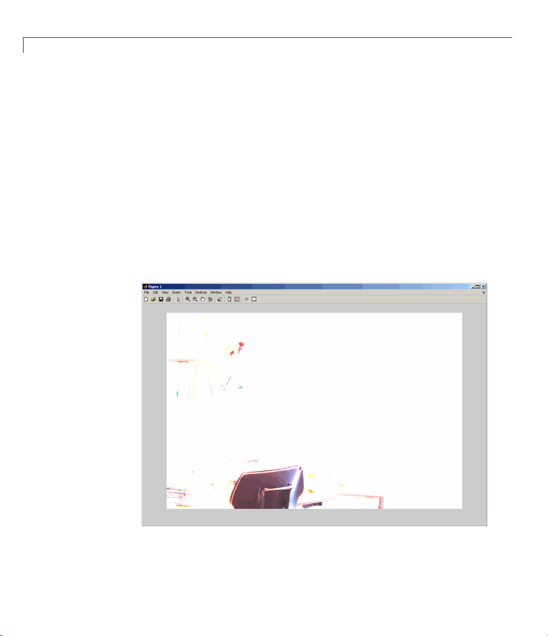
3 Reading and Writing Image Data

image. For more information, see “Viewing a High Dynamic Range Image” on page 3-22.

Creating a High Dynamic Range Image

To create a high dynamic range image from a group of low dynamic range images, use the must be spatially registered and the image files must contain EXIF metadata. Specify the low-dynamic range images in a cell array.

hdr_image = makehdr(files);

Viewing a High Dynamic Range Image

If you try to view a HDR image using imshow, the image does not display correctly.

makehdr function. Note that the low dynamic range images

3-22

To view an HDR image, you must first convert the data to a dynamic range that can be displayed correctly on a computer. Use the

tonemap function to

Working with High Dynamic Range Images

perform this conversion. tonemap converts the high dynamic range image into an RGB image of class

rgb = tonemap(hdr_image);

whos

Name Size Bytes Class Attributes

hdr_image 665x1000x3 7980000 single rgb 665x1000x3 1995000 uint8

uint8.

After converting the HDR image, try to display the image again.

imshow(rgb);

Writing a High Dynamic Range Image to a File

To write a high dynamic range image from the MATLAB workspace into a file, use the

hdrwrite function.

3-23

3 Reading and Writing Image Data

hdrwrite(hdr,'filename');

3-24

Mathworks IMAGE PROCESSING TOOLBOX 7 user guide

Specifications and Main Features

Frequently Asked Questions

User Manual

Getting Started

Product Overview

Introduction

Configuration Notes

Related Products

Compilability

Example 1 — Reading and Writing Images

Introduction

Step 1: Read and Display an Image

Step 2: Check How the Image Appears in the Workspace

Step 3: Improve Image Contrast

Step4: WritetheImagetoaDiskFile

Step 5: Check the Contents of the Newly Written File

Example 2 — Analyzing Images

Introduction

Step 2: Use Morphological Opening to Estimate the Background

Step 3: View the Background Approximation as a Surface

Step 4: Subtract the Background Image from the Original Image

Step 7: Identify Objects in the Image

Step 8: Examine One Object

Step 10: Compute Area of Each Object

Step 12: Create Histogram of the Area

Getting Help

Product Documentation

Image Processing Demos

MATLAB Newsgroup

Image Credits

Introduction

Images in MATLAB

Image Coordinate Systems

Pixel Coordinates

Spatial Coordinates

Using a Non-Default Spatial Coordinate System

ImageTypesintheToolbox

Overview of Image Types

Binary Images

Indexed Images

Converting Between Image Types

Converting Between Image Classes

Overview of Image Class Conversions

Losing Information in Conversions

Converting Indexed Images

Working with Image Sequences

Overview of Toolbox Functions That Work with Image Sequences

Example: Processing Image Sequences

Multi-Frame Image Arrays

Image Arithmetic

Overview of Image Arithmetic Functions

Reading and Writing Image Data

Getting Information About a Graphics File

Reading Image Data

Writing Image Data to a File

Overview

Specifying Format-Specific Parameters

Reading and Writing Binary Images in 1-Bit Format

Determining the Storage Class of the Output File

Converting Between Graphics File F ormats

Working with DICOM Files

Overview of DICOM Support

Reading Metadata from a DICOM File

Handling Private Metadata

Creating Your Own Copy of the DICOM Dictionary

Reading Image Data from a DICOM File

Viewing Images from DICOM Files

Writing Image Data or Metadata to a DICOM File

Understanding Explicit Versus Implicit VR Attributes

Removing Confidential Information from a DICOM File

Example: Creating a New DICOM Series

Working with Mayo Ana lyze 7.5 Files

Working with Interfile Files

Working with High Dynamic Range Images

Overview

Reading a High Dynamic Range Image

Creating a High Dynamic Range Image

Viewing a High Dynamic Range Image

Writing a High Dynamic Range Image to a File