Mathworks FIXED-INCOME TOOLBOX 1 user guide

Download

Fixed-Income Tool

User’s Guide

box™ 1

How to Contact The MathWorks

www.mathworks. comp.soft-sys.matlab Newsgroup www.mathworks.com/contact_TS.html Technical Support

suggest@mathworks.com Product enhancement suggestions

bugs@mathwo doc@mathworks.com Documentation error reports service@mathworks.com Order status, license renewals, passcodes

info@mathwo

com

rks.com

Web

Bug reports

Sales, prici

ng, and general information

508-647-7000 (Phone)

508-647-7001 (Fax)

The MathWorks, Inc. 3 Apple Hill Drive Natick, MA 01760-2098

For contact information about worldwide offices, see the MathWorks Web site.

Fixed-Income Toolbox™ User’s Guide

The software described in this document is furnished under a license agreement. The software may be used or copied only under the terms of the license agreement. No part of this manual may be photocopied or reproduced in any form without prior written consent from The MathW orks, Inc.

FEDERAL ACQUISITION: This provision applies to all acquisitions of the Program and Documentation by, for, or through the federal government of the United States. By accepting delivery of the Program or Documentation, the government hereby agrees that this software or documentation qualifies as commercial computer software or commercial computer software documentation as such terms are used or defined in FAR 12.212, DFARS Part 227.72, and DFARS 252.227-7014. Accordingly, the terms and conditions of this Agreement and only those rights specified in this Agreement, shall pertain to and govern theuse,modification,reproduction,release,performance,display,anddisclosureoftheProgramand Documentation by the federal government (or other entity acquiring for or through the federal government) and shall supersede any conflicting contractual terms or conditions. If this License fails to meet the government’s needs or is inconsistent in any respect with federal procurement law, the government agrees to return the Program and Docu mentation, unused, to The MathWorks, Inc.

Trademarks

MATLAB and Simulink are registered trademarks of The MathWorks, Inc. See

www.mathworks.com/trademarks for a list of additional trademarks. Other product or brand

names may be trademarks or registered trademarks of their respective holders.

Patents

The MathWorks products are protected by one or more U.S. patents. Please see

www.mathworks.com/patents for more information.

Revision History

May 2003 Online only New for V ersion 1.0 (Release 13) November 2003 First printing Unchanged June 2004 Online only Revised for Version 1.0.1 (Release 14) August 2004 Online only Revised for Version 1.1 (Release 14+) September 2005 Online only Revised for Version 1.1.1 (Release 14SP3) March 2006 Online only Revised for Version 1.1.2 (Release 2006a) September 2006 Online only Revised for Version 1.2 (Release 2006b) March 2007 Online only Revised for Version 1.3 (Release 2007a) September 2007 Online only Revised for Version 1.4 (Release 2007b) March 2008 Online only Revised for Version 1.5 (Release 2008a) October 2008 Online only Revised for Version 1.6 (Release 2008b) March 2009 Online only Revised for Version 1.7 (Release 2009a) September 2009 Online only Revised for Version 1.8 (Release 2009b) March 2010 Online only Revised for Version 1.9 (Release 2010a)

Getting Started

Product Overview ................................. 1-2

Introduction Expected Background

...................................... 1-2

.............................. 1-2

Contents

What This Product Provides

Supported Tasks Using Mortgage-Backed Securities Using Debt Instruments Using Derivative Securities Using Interest-Rate Curve Objects

.................................. 1-4

........................ 1-4

................... 1-4

............................ 1-5

......................... 1-5

................... 1-5

Mortgage-Backed Securities

What Are Mortgage-Backed Securities? .............. 2-2

Using Fixed-Rate Mortgage Pool Functions

Introduction Inputs to Functions Generating Prepayment Vectors Mortgage Prepayments Risk Measurement Mortgage Pool Valuation Computing Option-Adjusted Spread Prepayments with Fewer Than 360 Months Remaining Pools with Different Numbers of Coupons Remaining

...................................... 2-3

................................ 2-4

..................... 2-4

............................. 2-6

................................ 2-8

........................... 2-9

.................. 2-10

.......... 2-3

.. 2-13

.... 2-15

Debt Instruments

Treasury Bills Defined ............................. 3-2

Computing T reasury Bill Price and Yield

Introduction Treasury Bill Repurchase Agreements Treasury Bill Yields

Using Zero-Coupon Bonds

Introduction Measuring Zero-Coupon Bond Function Quality PricingTreasuryNotes Pricing Corporate Bonds

Stepped-Coupon Bonds

Introduction Cash Flows from Stepped-Coupon Bonds Price and Yield of Stepped-Coupon Bonds

Term Structure Calculations

Introduction Computing Spot and Forward Curves Computing Spreads

...................................... 3-3

................ 3-3

............................... 3-5

.......................... 3-7

...................................... 3-7

............................. 3-8

............................ 3-10

............................ 3-12

...................................... 3-12

....................... 3-15

...................................... 3-15

................. 3-15

................................ 3-17

............ 3-3

........ 3-7

.............. 3-12

.............. 3-14

vi Contents

ing and Hedging

Pric

Pricing Assumptions

Swap

p Pricing Example

Swa

tfolio Hedging

Por

nvertible B on d Valuation

nd Fu tures

.................................

.....................................

Derivative Securities

...............................

..........................

.............................

........................

4-2 4-2 4-3 4-8

Supported Bond Futures ............................ 4-12

Example Analysis of Bond Futures Managing Interest-Rate Risk with Bond Futures

................... 4-14

........ 4-16

Interest-Rate Curve Objects

Introduction to Interest-Rate Curve Objects ......... 5-2

Class Structure Supported Workflow Model Using Interest-Rate Curve

Objects

................................... 5-2

........................................ 5-3

Creating Interest-Rate Curve Objects

Creating an IRDataCurve Object

Using the IRDataCurve Constructor with Dates and

Data

.......................................... 5-6

Using IRDataCurve bo otstrap Method for Bootstrapping

Based on Market Instruments

Creating an IRFunctionCurve Object

Using a Function Handle to Fit an IRFunctionCurve

Object

Using the Nelson-Siegel M ethod to Fit an IRFunctionCurve

Object

Using the Svensson Method to Fit an IRFunctionCurve

Object

UsingtheSmoothingSplineMethodtoFitan

IRFunctionCurve Object

Using the fitFunction to Create a Custom Fitting Function

for an IRFunctionCurve Object

Converting an IRDataCurve or IRFunctionCurve

Object

Introduction Using the toRateSpec Method Using Vector of Dates and Data Methods

......................................... 5-13

......................................... 5-14

......................................... 5-16

.......................................... 5-25

...................................... 5-25

..................... 5-7

.......................... 5-18

....................... 5-25

............... 5-4

.................... 5-6

................ 5-13

.................... 5-21

.............. 5-26

vii

Function Reference

Bond Futures ..................................... 6-2

Certificates of Deposit

Convertible Bonds

Derivative Securities

Interest-Rate Curve Objects

Mortgage-Backed Securities

Option-Adjusted Spread Computations

Stepped-Coupon Bonds

Treasury Bills

Zero-Coupon Instruments

..................................... 6-9

............................. 6-2

................................. 6-3

.............................. 6-3

........................ 6-3

........................ 6-6

............................ 6-8

.......................... 6-10

.............. 6-7

viii Contents

Functions — Alphabetical List

Class Reference

@IRBootstrapOptions .............................. A-2

Hierarchy Constructor

........................................ A-2

...................................... A-2

Public Read-Only Properties ........................ A-2

Methods

......................................... A-3

@IRCurve

Hierarchy Description Constructor Public Read-Only Properties Methods

@IRDataCurve

Hierarchy Description Constructor Public Read-Only Properties Methods

@IRFitOptions

Hierarchy Description Constructor Public Read-Only Properties Methods

@IRFunctionCurve

Hierarchy Description Constructor Public Read-Only Properties Methods

......................................... A-4

........................................ A-4

....................................... A-4

...................................... A-4

......................................... A-6

..................................... A-7

........................................ A-7

....................................... A-7

...................................... A-7

......................................... A-9

..................................... A-10

........................................ A-10

....................................... A-10

...................................... A-10

......................................... A-11

................................ A-12

........................................ A-12

....................................... A-12

...................................... A-12

......................................... A-14

........................ A-4

........................ A-8

........................ A-11

........................ A-13

Bibliography

Fitting Interest-Rate Curve Functions ............... B-2

Bootstrapping a Swap Curve

....................... B-3

Bond Futures ..................................... B-4

Examples

Treasury Bills ..................................... C-2

Using Zero-Coupon Bonds

Stepped-Coupon Bonds

Pricing and Hedging

Bond Futures

..................................... C-2

............................... C-2

.......................... C-2

............................ C-2

Glossary

Index

x Contents

Getting Started

• “Product Overview” on page 1-2

• “What This Product Provides” on page 1-4

1 Getting Started

Product Overview

Introduction

Fixed-Income Toolbox™ software extends MATLAB®with functions for fixed-income modeling and analysis. You can use the toolbox to determine the price, yield, and cash flow for many types of fixed-income securities, including mortgage-backed securities, corporate bonds, treasury bonds, municipal bonds, certificates of deposit, and treasury bills. Fixed-Income Toolbox functions also enable you to work with derivatives, including swaps, convertible bonds, and treasury futures. The built-in functions can be used to create customized fixed-income models based on mortgage-backed securities and debt instruments.

In this section...

“Introduction” on page 1-2

“Expected Background” on page 1-2

1-2

Expected Background

In general, this guide assumes experience working with fixed-income instruments and some familiarity with the underlying models.

Your title is likely one of these:

• Analyst, quantitative analyst

• Risk manager

• Portfolio manager

• Fund manager, asset m anager

• Financial engineer

• Trader

• Student, professor, or other academic

Your background, education, training, and responsibilities likely match some aspectsofthisprofile:

Product Overview

• Finance, economics, perhaps accounting

• Engineering, mathematics, physics, other quantitative sciences

• Bachelor’s degree minimum; MS or MBA likely; Ph.D. perhaps; CFA

• Comfortable with probability theory, statistics, and algebra

• Understand linear or matrix algebra and calculus

• Perhaps new to MATLAB software

1-3

1 Getting Started

What This Product Provides

In this section...

“Supported Tasks” on page 1-4

“Using Mortgage-Backed Securities” on page 1-4

“Using Debt Instruments” on page 1-5

“Using Derivative Securities” on page 1-5

“Using Interest-Rate Curve Objects” on page 1-5

Supported Tasks

Fixed-Income Toolbox software extends MATLAB software with functions for fixed-income modeling and analysis. You can use the toolbox to determine the price, yield, and cash flow for many types of fixed-income securities, including mortgage-backed securities, corporate bonds, Treasury bonds, municipal bonds, certificates of deposit, and Treasury bills.

1-4

Fixed-Income Toolbox software also enables y ou to work with derivatives, including swaps, convertible bonds, and Treasury futures. You can use built-in functions to create customized fixed-income models based on mortgage-backed securities and debt instruments. You can then use Fixed-Income Toolbox softwaretoperformthefollowing:

• Calculate the price and yield for generic fixed-rate mortgage pools and

balloon mortgages.

• Determine the price, yield, discount rate, and cash-flow schedule for

debt instruments, including Treasury bills, zero-coupon bonds, and stepped-coupon bonds.

• Calculate swap rates and sensitivities.

• Analyze the term structure of interest rates, including bootstrapping and

fitting the term structure to market data using parametric models.

Using Mortgage-Backed Securities

With Fixed-Income Toolbox software, you can model generic fixed-rate mortgage pools and balloon mortgages. Tools are provided for:

What This Product Provides

• Calculating the price and yield of mortgage-backed securities using

prepayment options derived from uniform practices of the Public Securities Association (PSA)

• Determining the mortgage-pool price or effective duration using the

option-adjusted spread (OAS) method

• Calculating basic risk measurements for a mortgage-pool portfolio using

convexity, duration, and average life

Using Debt Instruments

You can also use Fixed-Income Toolbox software to work with a variety of debt instruments. You can calculate price, yield, dis count rate, and break-even discount rate for treasury bills, and determine price, yield, and cash- flow schedules for corporate, treasury, and municipal bonds. The zero-coupon functions in Fixed-Income Toolbox software help with the extraction of present value from virtually any fixed-coupon instrument for any time period. Toolbox functions also let you calculate price, yield, and cash-flow schedules for stepped-coupon bonds. The n ext coupon dates are computed automatically from the last entered input end dates. The payment due on settlement represents the accrued interest due on that day.

Using Derivative Securities

In addition, Fixed-Income Toolbox software provides tools based on Black’s option functions for working with fixed-income derivatives. These tools let you calculate swap price by computing par yields that equate the floating-rate side of a swap to the fixed-rate side. You can set the present value of the fixed side to the present value of the floating side without aligning and comparing fixed and floating periods. The duration-hedging capability in the toolbox lets you hedge a portfolio and address interest-rate risk exposure with a swap arrangement. Fixed-Income Toolbox software lets you use binomial a nd trinomial trees to v a lue convertible bonds. The value of the convertible bond is determined by the uncertainty of the relative stock.

Using Interest-Rate Curve Objects

Fixed-Income Toolbox software provides tools for analyzing the term structure of interest rates, including bootstrapping and fitting the term structure to market data using parametric models (e.g., Nelson-Siegel and Svensson),

1-5

1 Getting Started

spline-based models, and user-defined functions. Fixed-Income Toolbox supports three class objects:

• “@IRCurve” on page A-4

Creates an interest-rate curves and includes methods for extracting forward, zero, and discount factors curves.

Supports a method to convert to a acceptable input format for the Financial Derivatives Toolbox™ function

intenvset.

• “@IRDataCurve” on page A-7

Represents interest-rate curves based on vectors of dates and data. This class supports bootstrapping an interest-rate curve from market instruments with a range of interpolation methods.

• “@IRFunctionCurve” on page A-12

Represents an interest-rate curve with a function; the function can be specified directly, or a form of the function can be specified and then the parameters are fit to available market data. In addition, you can determine which type of interest-rate curve (zero, forward, or discount curve) fits the market data, as well as, any custom functions.

RateSpec structure, which is an

1-6

Mortgage-Backed Securities

• “What Are Mortgage-Backed Securities?” on page 2-2

• “Using Fixed-Rate Mortgage Pool Functions” on page 2-3

2 Mortgage-Backed Securities

What Are Mor tgage-Backed Securities?

Mortgage-backed securities (MBSs) are a type of investment that represents ownership in a group of mortgages. Principal and interest from the individual mortgages are used to pay principal and interest on the MBS.

Ownership in a group of mortgages is typically represented by a pass-through certificate (PC). Most pass-through certificates are issued by the Government National Mortgage Agency, a branch of the United States government, or by one of two private corporations: Fannie Mae or Freddie Mac. With these certificates, homeowners’ payments pass from the originating bank through the issuing agency to holders of the certificates. These agencies also frequently guarantee that the ce rtificate holder receives timely payment of principal and interest from the PCs.

2-2

Using Fixed-Rate Mortgage Pool Functions

In this section...

“Introduction” on page 2-3

“Inputs to Functions” on page 2-4

“Generating Prepayment Vectors” on page 2-4

“Mortgage Prepayments” on page 2-6

“Risk Measurement” on page 2-8

“Mortgage Pool Valuation” on page 2-9

“Computing Option-Adjusted Spread” on page 2-10

“Prepayments with Fewer Than 360 Months Remaining” on page 2-13

“Pools with Different Numbers of Coupons Remaining” on page 2-15

Introduction

Fixed-Income Toolbox software supports calculations involved with generic fixed-rate mortgage pools and balloon mortgages. Pass-through certificates typically ha ve embedded call options in the form of prepayment. Prepayment is an excess payment applied to the principal of a PC. These accelerated payments reduce the effective life of a PC.

The toolbox comes with a sta n da rd Bond Market Association (PSA) prepayment model and can generate multiples of standard prepayment speeds. The Public Securities Association provides a set of uniform practices for calculating the characteristics of mortgage-backed securities when there is an assumed prepayment function.

You can obtain more information about these uniform practices on the PSA Web site (

Alternatively, aside from the standard PSA implementation in this toolbox, you can supply yo ur own projected prepayment vectors. At this time, however, custom prepayment functionality that incorporates pool-specific information and interest rate forecasts are not available in this toolbox. If you plan to use

http://www.bondmarkets.com).

2-3

2 Mortgage-Backed Securities

custom prepayment vectors in your calculations, you presumably already own such a suite in MATLAB.

Inputs to Functions

Because of the generic, all-purpos e nature of the toolbox pass-through functions, you can fine-tune them to conform to a particular mortgage. Most functions require at least this set of inputs:

• Gross coupon rate

• Settlement date

• Issue (effective) date

• Maturity date

Typical optional inputs include standard prepay m en t speed (or customized vector), net coupon rate (if different from gross coupon rate), and payment delay in number of days.

2-4

All calculations are based on expected payment dates and actual cash flow to the investor. For example, when to

mbsdurp, the function returns a modified duration based on CouponRate.

(A notable exception is based on the

GrossRate.)

mbspassthrough, which returns interest quantities

GrossRate and CouponRate differ as inputs

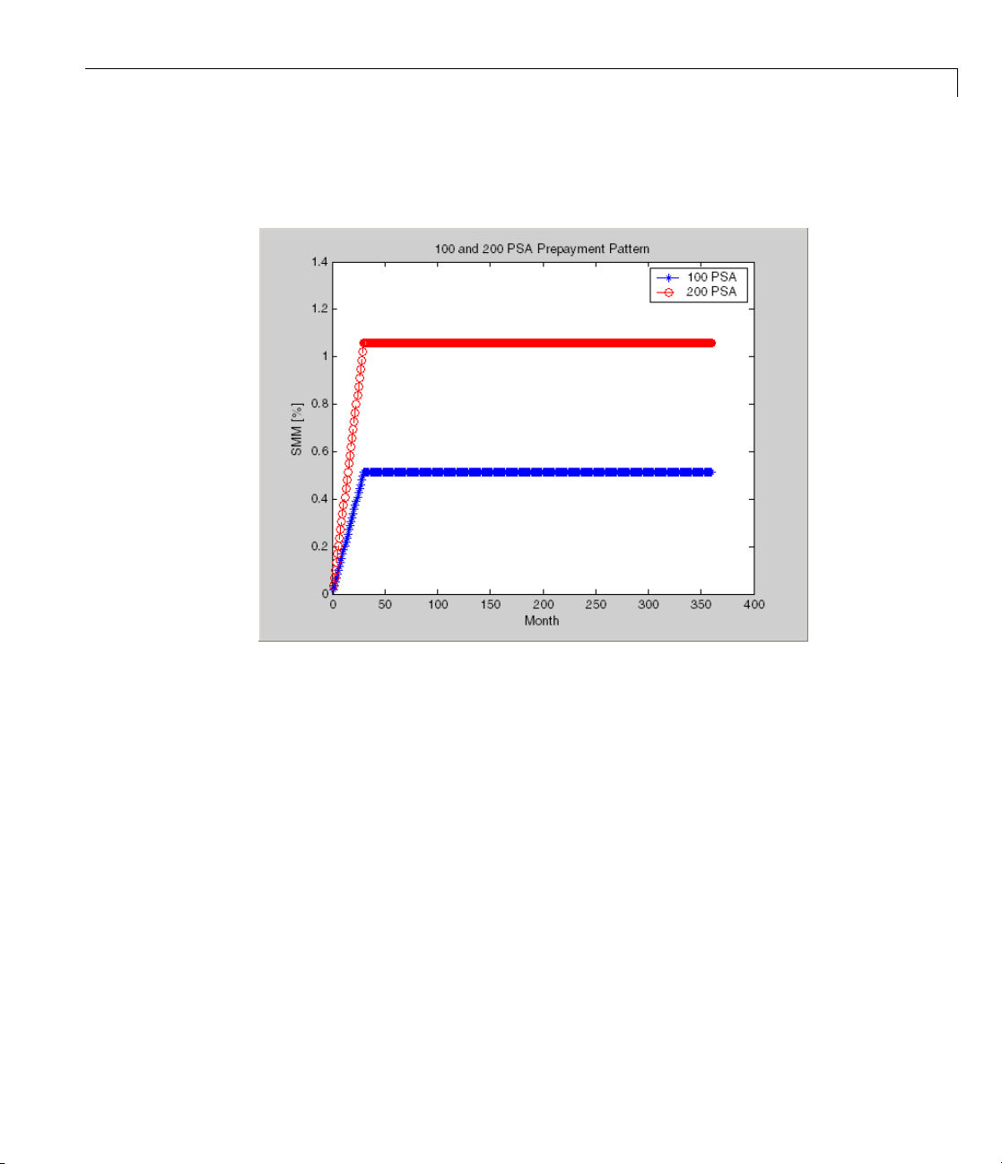
Generating Prepayment Vectors

You can generate PSA multiple prepayment vectors quickly. T o generate prepayment vectors of 100 and 200 PSA, type

PSASpeed = [100, 200]; [CPR, SMM] = psaspeed2rate (PSASpeed);

This function computes two prepayment values: conditional prepayment rate (CPR) and single monthly mortality (SMM) rate. CPR is the percentage of outstanding principal prepaid in1year. SMMisthepercentageof outstanding principal prepaid in 1 month. In other words, CPR is an annual version of SMM.

Using Fixed-Rate Mortgage Pool Functions

Since the entire 360-by-2 array is too long to show in this document, observe the SMM (100 and 200 PSA) plots, spaced one month apart, instead.

Prepayment assumptions form the basis upon which far more comprehensive MBS calculations are based. As an illustration observe the following example, which shows the use of the function

mbscfamounts to generate cash flows and

timings based on a set of standard prepayments.

Considerthreemortgagepoolsthatweresoldontheissuedate(whichstarts unamortized). The first two pools "balloon out" in 60 months, and the third is regularly amortized to the end. The prepayment speeds are assumed to be 100, 200, and 200 PSA, respectively.

Settle = [datenum('1-Feb-2000');

datenum('1-Feb-2000'); datenum('1-Feb-2000')];

Maturity = [datenum('1-F eb-2030')];

IssueDate = datenum('1-Feb-2000');

2-5

2 Mortgage-Backed Securities

The fourth output argument, Factors, indicates the fraction of the balance still outstanding at the beginning of each month. A snapshot of this argument in the MATLAB Variable Editor illustrates the 60-month life of the first two of the mortgages with balloon payments and the continuation of the third mortgage until the end (360 months).

GrossRate = 0.08125; CouponRate = 0.075; Delay = 14;

PSASpeed = [100, 200]; [CPR, SMM] = psaspeed2rate (PSASpeed);

PrepayMatrix = ones(360,3); PrepayMatrix(1:60,1:2) = SMM(1:60,1:2); PrepayMatrix(:,3) = SMM(:,2);

[CFlowAmounts, CFlowDates, TFactors, Factors] = . .. mbscfamounts(Settle, Maturity, IssueDate, GrossRate, ... CouponRate, Delay, [], PrepayMatrix);

2-6

You can readily see that mbscfamounts is the building block of most fixed rate and balloon pool cash flows.

Mortgage Prepayments

Prepayment is beneficial to the pass-through owner when a mortgage pool has been p urchased at discount. The next example compares mortgage yields (compounded monthly) versus the purchase clean price with constant

Using Fixed-Rate Mortgage Pool Functions

prepayment speed. The example illustrates that when you have purchased a pool at a discount, prepay m ent generates a higher yield with decreasing purchase price.

Price = [85; 90; 95]; Settle = datenum('15-Apr-2002'); Maturity = datenum('1 Jan 2030'); IssueDate = datenum('1-Jan-2000'); GrossRate = 0.08125; CouponRate = 0.075; Delay = 14; Speed = 100;

Compute the mortgage and bond-equivalent yields.

[MYield, BEMBSYield] = mb syield(Price, Settle, Maturity, ... IssueDate, GrossRate, CouponRate, Delay, Speed)

MYield =

0.1018

0.0918

0.0828

BEMBSYield =

0.1040

0.0936

0.0842

If for this same pool of mortgages, there was no prepayment (Speed = 0), the yields would decline to

MYield =

0.0926

0.0861

0.0802

BEMBSYield =

2-7

2 Mortgage-Backed Securities

Likewise, if the rate of prepayment doubled (Speed = 200), the yields would increase to

0.0944

0.0877

0.0815

MYield =

0.1124

0.0984

0.0858

BEMBSYield =

0.1151

0.1004

0.0873

2-8

For the same prepayment vector, deeper discount pools earn higher yields. For more information, see

mbsprice and mbsyield.

Risk Measurement

Fixed-Income Toolbox software provides the most basic risk measures of a pool portfolio:

• Modified duration

• Convexity

• Averagelifeofpool

Consider the following ex ample, which calculates the Macaulay and modified durations given the price of a mortgage pool.

Price = [95; 100; 105]; Settle = datenum('15-Apr-2002'); Maturity = datenum('1-Jan-2030'); IssueDate = datenum('1-Jan-2000'); GrossRate = 0.08125;

Using Fixed-Rate Mortgage Pool Functions

CouponRate = 0.075; Delay = 14; Speed = 100;

[YearDuration, ModDuration] = mbsdurp(Price, Settle, ... Maturity, IssueDate, GrossRate, CouponRate, Delay, Speed)

YearDuration =

6.1341

6.3882

6.6339

ModDuration =

5.8863

6.1552

6.4159

Using Fixed-Income Toolbox functions, you can obtain modified duration and convexity from either price or yield, as long as you specify a prepayment vector or an assumed prepayment speed. The toolbox risk-measurement functions (

mbsdurp, mbsdury, mbsconvp, mbsconvy,andmbswal)adheretothe

guidelines listed in the PSA Uniform Practices manual.

Mortgage Pool Valuation

For accurate valuation of a mortgage pool, you must generate interest rate paths and use them with mortgage pool characteristics to properly value the pool. A widely used methodology is the option-adjusted spread (OAS). OAS measures the yield spread that is not directly attributable to the characteristics of a fixed-income investment.

Calculating OAS

Prepayment alters the cash flows of an otherwise regularly amortizing mortgage pool. A comprehensive option-adjusted spread calculation typically begins with the generation of a set of paths of spot rates to predict prepayment. A path is collection of i spot-rate paths, with corresponding j cashflowsoneachofthosepaths.

2-9

2 Mortgage-Backed Securities

The effect of the OAS on pool pricing is shown mathematically in the following equation, where K is the option-adjuste d spread.

∑

1()

zerorates K

PoolPrice

mmberofPaths

=×

NumberofPaths

∑

Calculating Effective Duration

Alternatively, if you are more interested in the sensitivity of a mortgage pool to interest rate changes, use effective duration, which is a more appropriate measure. Effective duration is defined mathematically with the following equation.

+− −()()

ΔΔ

Py y Py y

Effective Duration

()

Δ2

Py y

Calculating Market Price

The toolbox has all the components required to calculate OAS and effective duration if you supply prepayment vectors or assumptions. For O AS, given a prepayment vector, you can generate a set of cash flows with Discounting these cash flows with the reference curve and then adding OAS produces the market price. See “Computing Option-Adjusted Spread” on page 2-10 fo r a discussion on the computation of option-adjusted spread.

Effective duration is a more difficult issue. W hile modified duration changes the discounting process (by changing the yield used to discount cash flows), effective duration must account for the change in cash flow because of the change in yield. A possible solution is to recompute prices using a small change in yield, in both the upwards and downwards directions. In this case, you must recompute the prepayment input. Internally, this alters the cash flows of the mortgage pool. Assuming that the OAS stays constant in all yield environments, you can apply a set of discounting factors to the cash flows in up and down yield environments to find the effective duration.

mbscfamounts.

mbsprice for

2-10

Computing Option-Adjusted Spread

The option-adjuste d spread (OAS) is an amount of extra interest added above (orbelowifnegative)thereferencezerocurve. TocomputetheOAS,youmust

Using Fixed-Rate Mortgage Pool Functions

provide the zero curve as an extra input. You can specify the zero curve in any intervals and with any compounding method. (To minimize any error due to interpolation, keep the intervals as regular and frequent as possible.) You must supply a prepayment vector or specify a speed corresponding to a standard PSA prepayment vector.

Onewaytocomputetheappropriatezerocurveforanagencyistolookatits bond yields and bootstrap them from the shortest m aturity onwards. You can do this with Financial Toolb ox™ functions

zbtprice and zbtyield.

The following example shows how to calculate an appropriate zero curve followed by computation of the pool’s OAS. This example calculates the OAS of a 30-year fixed rate mortgage with about a 28-year w eigh t ed average maturity left, given an assumption of 0, 50, and 100 PSA prepayment speeds.

Create curve for

Bonds = [datenum('11/21/2002') 0 100 0 2 1;

Yields = [0.0162;

zerorates.

datenum('02/20/2003') 0 100 0 2 1;

datenum('07/31/2004') 0.03 100 2 3 1;

datenum('08/15/2007') 0.035 100 2 3 1;

datenum('08/15/2012') 0.04875 100 2 3 1;

datenum('02/15/2031') 0.05375 100 2 3 1];

0.0163;

0.0211;

0.0328;

0.0420;

0.0501];

Since the above is Treasury data and not selected agency data, a term structure of spread is assumed. In this example, the spread declines proportionally from a maximum of 250 basis points at the shortest maturity.

Yields = Yields + 0.025 * (1./[1:6]');

Get parameters from Bonds matrix.

Settle = datenum('20-Aug-2002');

Maturity = Bonds(:,1);

2-11

2 Mortgage-Backed Securities

Use zbtprice to solve for zero rates.

Use output from zbtprice to calculate the OAS.

CouponRate = Bonds(:,2);

Face = Bonds(:,3);

Period = Bonds(:,4);

Basis = Bonds(:,5);

EndMonthRule = Bonds(:,6);

[Prices, AccruedInterest] = bndprice(Yields, CouponRate, ...

Settle, Maturity, Period, Basis, EndMonthRule, [], [], [], [], ...

Face);

[ZeroRatesP, CurveDatesP] = zbtprice(Bonds, Prices, Settle); ZeroCompounding = 2*ones(size(ZeroRatesP)); ZeroMatrix = [CurveDatesP, ZeroRatesP, ZeroCompounding];

Price = 95; Settle = datenum('20-Aug-2002'); Maturity = datenum('2-Jan-2030'); IssueDate = datenum('2-Jan-2000'); GrossRate = 0.08125; CouponRate = 0.075; Delay = 14; Interpolation = 1; PrepaySpeed = [0; 50; 100];

2-12

OAS = mbsprice2oas(ZeroMatrix, Price, Settle, Maturity, ... IssueDate, GrossRate, CouponRate, Delay, Interpolation, ... PrepaySpeed)

OAS =

26.0502

28.6348

31.2222

This example shows that one cash flow set is being discounted and solved for its OAS, as contrasted with the

NumberOfPaths set of cash flows as shown

Using Fixed-Rate Mortgage Pool Functions

in “Mortgage Pool Valuation” on page 2-9. Averaging the sets of cash flows resulting from all simulations into one average cash flow vector and solving for the OAS, discounts the averaged cash flows to have a present value of today’s (average) price.

While this example uses the mortgage pool price ( theOAS,youcanalsouseyieldtoresolveit( reverse OAS functions that return prices and yields given OAS ( and mbsoas2yield).

The example also restates earlier examples that show discount securities benefit from higher l evel of prepayme nt, keeping everything else unchanged. The relation is reversed for premium securities.

mbsprice2oas) to determine

mbsyield2oas). Also, there are

mbsoas2price

Prepayments with Fewer Than 360 Months Remaining

When fewer than 360 months remain in the pool, the applicable PSA prepayment vector is "seasoned" by the pool’s age. (Elements in the 360-element prepayment vector that repres ent past payments are skipped. For example, on a 30-year mortgage that is 10 months old, only the final 350 prepayments are applied.)

Assume, for example, that you h ave two 30-year loans, one new and another 10 months old. Both have the same PSA speed of 100 and prepay using the vectors plotted below.

2-13

2 M ortgage-Backed Securities

2-14

Still within the scope of relative valuation, you could also solve for the percentage of the standard PSA prepayment vector given the pool’s arbitrary, user-supplied prepayment vector, such that the PSA speed gives the same Macaulay duration as the user-supplied prepayment vector.

If yo u supply a custom prepayment vector, you must account for the number of months remaining.

Price = 101; Settle = datenum('1-Jan-2001'); Maturity = datenum('1-Jan-2030'); IssueDate = datenum('1-Jan-2000'); GrossRate = 0.08125; PrepayMatrix = 0.005*ones(348,1); CouponRate = 0.075; Delay = 14;

ImpliedSpeed = mbsprice2speed(Price, Settle, Maturity, ... IssueDate, GrossRate, PrepayMatrix, CouponRate, Delay)

Using Fixed-Rate Mortgage Pool Functions

ImpliedSpeed =

104.2526

Examine the prepayment input. The remaining 29 years require 348 monthly elements in the prepayment vector. Supposethen,keepingeverythingthe same, you change

Settle = datenum('14-Feb-2003');

Settle to February 14, 2003.

You can use cpncount to count all incoming coupons received after Settle by invoking

NumCouponsRemaining = cpncount(Settle, Maturity, 12, 1, [], ... IssueDate)

NumCouponsRemaining = 323

The input 12 defines the monthly payment frequency, 1 defines the 30/360 basis, and

IssueDate defines aging and determination-of-holder date.

Thus, you must supply a 323-element vector to account for a prepayment corresponding to each monthly payment.

Pools with Different Numbers of Coupons Remaining

Suppose one pool has two remaining coupons, and the other has three. MATLAB software expects the prepaymentmatrixtobeinthefollowing format:

V11 V21 V12 V22 NaN V23

denotes the single monthly mortality (SMM) rate for pool i during the jth

coupon period since

The use of

NaN to pad the prepayment matrix is necessary because MATLAB

cannot concatenate vectors of different lengths into a matrix. Also, it can

Settle.

2-15

2 M ortgage-Backed Securities

serve as an error check against any unintended operation (any MATLAB operation that would return

For example, assume that the 2 month pool has a constant SMM of 0.5% and the 3 month has a constant SMM of 1% in every period. The prepayment matrix you would create is depicted below.

NaN).

2-16

Create this input in whatever manner is best for you.

Summary of Prepayment Data Vector Representation

• When you specify a PSA prepayment speed, MATLAB "seasons" the pool

according to its age.

• Whenyouspecifyyourownprepayment matrix, identify the maximum

number of coupons remaining using elements up to the point when cash flow ceases to exist.

• When different length pools must exist inthesamematrix,padtheshorter

one(s) with specific pool.

NaN. Each column of the prepayment matrix corresponds to a

cpncount. Then supply the matrix

Debt Instruments

• “Treasury Bills Defined” on page 3-2

• “Computing Treasury Bill Price and Yield” on page 3-3

• “Using Zero-Coupon Bonds” on page 3-7

• “Stepped-Coupon Bonds” on page 3-12

• “Term Structure Calculations” on page 3-15

3 Debt Instruments

Treasury Bills Defined

Treasury bills are short-term securities (issued with maturities of 1 year or less) sold by the United States Treasury. Sales of these securities are frequent, usually week ly. F rom time to time, the Treasury also offers longer duration securities called Treasury notes and Treasury bonds.

A Treasury bill is a discount security. The holder of the Treasury bill does not receive periodic interest paym ents. Instead,atthetimeofsale,apercentage discount is applied to the face value. At maturity, the holder redeems the bill for full face value.

The basis for Treasury bill interest calculation is actual/360. Under this system, interest accrues on the actual number of e lapsed days between purchase and maturity, and each year contains 360 days.

3-2

Computing Treasury Bill Price and Yield

In this section...

“Introduction” on page 3-3

“Treasury Bill Repurchase Agreements” on page 3-3

“Treasury Bill Yields” on page 3-5

Introduction

Fixed-Income Toolbox software provides the following suite of functions for computing price and yield on Treasury bills.

Treasury Bill Function s

Function Purpose

tbilldi

tbillpr

tbillrepo

tbillyield

tbillyield2disc

tbillval01

sc2yield

ice

Convert d

Price Treasury bill given its yield or discount rate.

Break-even discount of repurchase agreement.

Yield and discount of Treasury bill given its price.

Convert yield to discount rate.

The value of 1 basis point given the characteristics of the Treasury bill, as represented by its settlement and maturity dates. You can relate the basis point to d iscount, money-market, or bond-equivalent yield.

iscount rate to yield.

Computing Treasury Bill Price a n d Yield

For all functions with yield in the computation, you can specify yield as money-market or bond-equivalent yield. The functions all assume a face value of $100 for each Treasury bill.

Treasury Bill Repurchase Agreements

The following example shows how to compute the break-even discount rate. This is the rate that correctly prices the Treasury bill such that the profit from selling the tail equ als 0.

3-3

3 Debt Instruments

Maturity = '26-Dec-2002'; InitialDiscount = 0.0161; PurchaseDate = '26-Sep-2002'; SaleDate = '26-Oct-2002'; RepoRate = 0.0149;

BreakevenDiscount = tbillrepo(RepoRate, InitialDiscount, ... PurchaseDate, SaleDate, Maturity)

BreakevenDiscount =

0.0167

You can check the result of this computation by examining the cash flows in and out from the repurchase transaction. First compute the price of the Treasury bill on the purchase date (September 26).

PriceOnPurchaseDate = tbillprice(InitialDiscount, ... PurchaseDate, Maturity, 3)

3-4

PriceOnPurchaseDate =

99.5930

Next compute the interest due on the repurchase agreement.

RepoInterest = ... RepoRate*PriceOnPurchaseDate*days360(PurchaseDate,SaleDate)/360

RepoInterest =

0.1237

RepoInterest

for a 1.49% 30-day term repurchase agreement (30/360 basis)

is 0.1237.

Finally,computethepriceoftheTreasurybillonthesaledate(October26).

PriceOnSaleDate = tbillprice(BreakevenDiscount, SaleDate, ... Maturity, 3)

Computing Treasury Bill Price a n d Yield

PriceOnSaleDate =

99.7167

Examining the cash flows, observe that the break-even discount causes the sum of the price on the purchase date plus the accrued 30-day interest to be equaltothepriceonsaledate. Thenexttableshowsthecashflows.

Cash Flows from Repurchase Agreement

Date CashOutFlow CashInFlow

9/26/2002

10/26/2002

Purchase T-bill

Payment of repo

Repo interest

99.593

0.1238

Repo m oney

Sell T-bill

99.593

99.7168

Total

199.3098 199.3098

Treasury Bill Yields

Using the same data as before, you can examine the money-market and bond-equivalent yields of the Treasury bill at the time of purchase and sale. The function

Maturity = '26-Dec-2002'; InitialDiscount = 0.0161; PurchaseDate = '26-Sep-2002'; SaleDate = '26-Oct-2002'; RepoRate = 0.0149; BreakevenDiscount = tbillrepo(RepoRate, InitialDiscount, ... PurchaseDate, SaleDate, Maturity)

[BEYield, MMYield] = ... tbilldisc2yield([InitialDiscount; BreakevenDiscount], ... [PurchaseDate; SaleDate], Maturity)

BreakevenDiscount =

tbilldisc2yield can perform both computations at one time.

3-5

3 Debt Instruments

0.0167

BEYield =

0.0164

0.0170

MMYield =

0.0162

0.0168

For the short Treasury bill (fewer than 182 days to m aturity), the money-market yield is 360/365 of the bond-equivalent yield, as this example shows.

3-6

Using Zero-Coupon Bonds

In this section...

“Introduction” on page 3-7

“Measuring Zero-Coupon Bond Function Quality” on page 3-7

“Pricing Treasury Notes” on page 3-8

“Pricing Corporate Bonds” on page 3-10

Introduction

A zero-coupon bond is a corporate, Treasury, or municipal debt instrument that pays no periodic interest. T ypically, the bond is redeemed at maturity for its full face value. It will be a security issued at a discount from its face value, or it may be a coupon bond stripped o f its coupons and repackaged as a zero-coupon bond.

Fixed-Income Toolbox software provides functions for valuing zero-coupon debt instruments. These functions supplement existing coupon bond functions such as software.

bndprice and bndyield that are available in Financial Toolbox

Using Zero-Coupon Bonds

Measuring Zero-Coupon Bond Function Quality

Zero-coupon function quality is measured by h ow consistent the results are with coupon-bearing bonds. Because the zero coupon’s yield is bond-equivalent, comparisons with coupon-bearing bonds are possible.

In the textbook case, where time (t) is measured continuously and the rate (r) is continuously compounded, the value of a zero bond is the principal

tiplied by

mul

be variable, requiring a more consistent approach to meet the stricter

can

ands of accurate pricing.

dem

e following two examples

rt−

. In reality, the rate quoted is continuous and the basis

3-7

3 Debt Instruments

• “Pricing Treasury Notes” on page 3-8

• “Pricing Corporate Bonds” on page 3-10

show how the zero functions are consistent with supported coupon bond functions.

Pricing Treasury Notes

A Treasury note can be considered to be a package of zeros. The toolbox functions that price zeros require a coupon bond equivalent yield. That yield can originate from any type of coupon paying bond, with any periodic payment, or any accrual basis. The next example shows the use of the toolbox to price a Treasury note and compares the calculated price with the actual price quotation for that day.

Settle = datenum('02-03-2003'); MaturityCpn = datenum('05-15-2009'); Period = 2; Basis = 0;

3-8

% Quoted yield. QYield = 0.03342;

% Quoted price. QPriceACT = 112.127;

CouponRate = 0.055;

Extract the cash flow and compute price from the sum of zeros discounted.

[CFlows, CDates] = cfa mounts(CouponRate, Settle, MaturityCpn, ...

Period, Basis);

MaturityofZeros = CDates;

Compute the price of the coupon bond identically a s a collection of zeros by multiplying the disco unt factors to the corresponding cash flows.

PriceofZeros = CFlows * zeroprice(QYi eld, Settle, .. . MaturityofZeros, Period, Basis)/100;

The following table shows the intermediate calculations.

Discounted Cash

Cash Flows Discount Factors

Flows

-1.2155 1.0000 -1.2155

2.7500 0.9908 2.7246

2.7500 0.9745 2.6799

2.7500 0.9585 2.6359

2.7500 0.9427 2.5925

2.7500 0.9272 2.5499

2.7500 0.9120 2.5080

2.7500 0.8970 2.4668

2.7500 0.8823 2.4263

2.7500 0.8678 2.3864

2.7500 0.8535 2.3472

2.7500 0.8395 2.3086

2.7500 0.8257 2.2706

102.7500 0.8121 83.4451

Total

112.1263

Using Zero-Coupon Bonds

Compare the quoted price and the calculated p rice based on zeros.

[QPriceACT PriceofZeros]

ans =

112.1270 112 .1263

This example shows that zeropr ice can satisfactorily price a Treasury note, a semiannual actual/actual basis bond, as if it were a composed of a series of zero-coupon bonds.

3-9

3 Debt Instruments

Pricing Corpora

You can similarl zero-coupon bon zeros exist. Yo quoted coupon-

Settle = datenum('02-05-2003'); MaturityCpn = datenum('01-14-2009'); Period = 2; Basis = 1; % Quoted yield. QYield = 0.05974; % Quoted price. QPrice30 = 99.382; CouponRate = 0.05850;

Extract ca

[CFlows, CDates] = cfa mounts(CouponRate, Settle, MaturityCpn, ...

Period, Basis);

Maturity = CDates;

Compute multip

the price of the coupon bond identically as a collection of zeros by

lying the discount factors to the corresponding cash flows.

y price a corporate bond, for which there is no corresponding

d, as opposed to a Treasury note, for which corresponding

u can create a synthetic zero-coupon bond and arrive at the

bond price when you later sum the zeros.

sh flow and compute price from the sum of zeros.

te Bonds

3-10

Price30 = CFlows * zeroprice(QYield, Settle, Mat urity, Period, ...

Basis)/100;

Compa

As a (

re quoted price and calculated price based on zeros.

[QPrice30 Price30]

ans =

99.3820 99.3 828

test of fidelity, intentionally giving the wrong basis, say actual/actual

sis = 0

) instead of 30/360, gives a price of 99.3972. Such a systematic

Using Zero-Coupon Bonds

error, if recurring in a more complex pric in g routine, quickly adds up to large inaccuracies.

In summ ary, the zero functions in MATLAB software facilitate extraction of present value from virtually any fixed-coupon instrument, up to any period in time.

3-11

3 Debt Instruments

Stepped-Coupon Bonds

In this section...

“Introduction” on page 3-12

“Cash Flows from Stepped-Coupon Bonds” on page 3-12

“Price and Yield of Stepped-Coupon Bonds” on page 3-14

Introduction

A stepped-coupon bond has a fixed schedule of changing coupon amounts. Like fixed coupon bonds, stepped-couponbondscouldhavedifferent periodic payments and accrual bases.

The functions such bonds. An accompanying function

stepcpnprice and stepcpnyield compute prices and yields of

stepcpncfamounts produces the cash

flow schedules pertaining to these bonds.

Cash Flows from Stepped-Coupon Bonds

Consider a bond that has a schedule of two coupons. Suppose the bond starts out with a 2% coupon that steps up to 4% in 2 years and onward to maturity. Assume that the issue and settlement dates are both March 15, 2003. The bond has a 5 year maturity. Use flow schedule and times.

Settle = datenum('15-Mar-2003');

Maturity = datenum('15-Mar-2008');

ConvDates = [datenum('15-Mar-2005')];

CouponRates = [0.02, 0. 04];

[CFlows, CDates, CTimes] = stepcpncfamounts(Settle, Maturity, ...

ConvDates, CouponRates)

Notably, ConvDates has 1 less element than CouponRates because MATLAB software assumes that the first element of schedule between

Settle (March 15, 2003) and the first element of ConvDates

(March 15, 2005), shown diagrammatically below.

stepcpncfamounts to generate the cash

CouponRates indicates the coupon

3-12

Stepped-Coupon Bonds

Effective 2% on March 15, 2003

Coupon Dates Semiannual Coupon Payment

15-Mar-03

15-Sep-03

15-Mar-04

15-Sep-04

15-Mar-05

15-Sep-05

15-Mar-06

15-Sep-06

15-Mar-07

15-Sep-07

15-Mar-08

Pay 2% from March 15, 2003

Pay 4% from March 15, 2003

Effective 4% on March 15, 2005

102

The payment on March 15, 2005 is still a 2% coupon. Payment of the 4% coupon starts with the next payment, September 15, 2005. March 15, 2005 is the end of first coupon schedule, not to be confused with the beginning of the second.

In summary, MATLAB takes user input as the end dates of coupon schedules and computes the next coupon dates automatically.

The payment due on settlement (zero in this case) represents the accrued interestdueonthatday. Itisnegative if such amount is nonzero. Comparison with

cfamounts in Financial Toolbox software shows that the two functions

operate identically.

3-13

3 Debt Instruments

Price and Yield of Stepped-Coupon Bonds

The toolbox provides two basic analytical functions to compute price and yield for stepped-coupon bonds. Using the above bond as an example, you can compute the price when the yield is known.

You can estimate the y ield to maturity as a number-of-year weighted average of coupon rates. For this b ond, the estimated yield is:

()()22 43

×+×

or 3.33%. While definitely not exact (due to nonlinear relation of price and yield), this estimate suggests close to par valuation and serves as a quick first check on the function.

Yield = 0.0333;

[Price, AccruedInterest] = stepcpnprice(Yield, Settle, ... Maturity, ConvDates, CouponRates)

3-14

The price returned is 99.2237 (per $100 notional), and the accrued interest is zero, consistent with our earlier assertions.

To validate that there is consistency among the stepped-coupon functions, you can use the above price and see if indeed it implies a 3.33% yield by using

stepcpnyield.

YTM = stepcpnyield(Price, Settle, Maturity, ConvDates, ... CouponRates)

YTM =

0.0333

Term Structure Calculations

In this section...

“Introduction” on page 3-15

“Computing Spot and Forward Curves” on page 3-15

“Computing Spreads” on page 3-17

Introduction

So far, a more formal definition of "yield" and its application has not been developed. In many situations when cash flow is available, discounting factors to the cash flows may not be immediately apparent. In other cases, what is relevant is often a spread, the difference between curves (also known as the term structure of spread).

All these calculations require one main ingredient, the Treasury spot, par-yield, or forward curve. Typically, the generation of these curves starts with a series of on-the-run and selected off-the-run issues as inputs.

Term S t ruct u re Ca l cula tion s

MATLAB software uses these bonds to find spot rates one at a time, from the shortest maturity onwards, using bootstrap techniques. All cash flows are used to construct the spot curve, and rates between maturities (for these coupons) are interpolated linearly.

Computing Spot and Forward Curves

For an illustration of how this works, observe the use of zbtyield (or equivalently

Bills Maturity Date Current Yield

3month

onth

zbtprice) on a portfolio of six Treasury bills and bonds.

7/03

4/1

7/17/03

1.1

1.18

3-15

3 Debt Instruments

Notes/Bonds

Coupon

2year 1.750

5year 3.000

10 year 4.000

30 year 5.375

Maturity Date

12/31/04

11/15/07

11/15/12

2/15/31

Current Yield

1.68

2.97

4.01

4.92

You can specify prices or yields to the bonds above to infer the spot curve. The function

To proceed, first assemble the above table into a variable called

zbtyield accepts yields (bond-equivalent yield, to be exact).

Bonds.The

first column contains maturities, the second contains coupons, and the third contains notionals or face values of the bonds. (Note that bills have zero coupons.)

Bonds = [datenum('04/17/2003') 0 100;

datenum('07/17/2003') 0 100; datenum('12/31/2004') 0.0175 100; datenum('11/15/2007') 0.03 100; datenum('11/15/2012') 0.04 100; datenum('02/15/2031') 0.05375 100];

Then specify the corresponding yields.

3-16

Yields = [0.0115;

0.0118;

0.0168;

0.0297;

0.0401;

0.0492];

You are now ready to compute the spot curve for each of these six maturities. The spot curve is based upon a settlement date of January 17, 2003.

Settle = datenum('17-Jan-2003'); [ZeroRates, CurveDates] = zbtyield(Bonds, Yields, Settle)

This gets you the Treasury spot curve for the day.

Term S t ruct u re Ca l cula tion s

You can compute the forward curve from this spot curve with zero2fwd.

[ForwardRates, CurveDates] = zero2fwd(ZeroRates, CurveDates, ...

Settle)

Here the notion of forward rates refers to rates between the maturity dates shown above, not to a certain period (forward 3 month rates, for example).

Computing Spreads

Calculating the spread between specific, fixed forward periods (such as the Treasury-Eurodollar spread) requires an extra step. Interpolate the zero rates (or zero prices, instead) for the corresponding maturities on the interval dates. Then use the interpolated zero rates to deduce the forward rates, and thus the spread of Eurodollar forward curve segments versus the relevant forward segments from Treasury bills.

3-17

3 Debt Instruments

Additionally, the variety of curve functions (including zero2fwd)helpsto standardize such calculations. For instance, by making both rates quoted with quarterly compounding and on an actual/360 basis, the resulting spread structure is fully comparable. This avoi ds the small inconsistency that occurs when directly comparing the bond-equ ivalent yield of a Treasury bill to the quarterly forward rates implied by Eurodollar futures.

Noise in Curve Computations

When introducing more bonds in constructing curves, noise may become a factor and may need some “smoothing” (with splines, for example); this helps obtain a s moother forward curve.

The following spot and forward curves are constructed from 67 Treasury bonds. The fitted and bootstrapped spot curve (bottom right figure) displays comparable stability. The forward curve (upper-left figure) contains significant noise and shows an improbable forward rate structure. The noise is not necessarily bad; it could uncover trading opportunities for a relative-value approach. Yet, a more balanced approach is desired when the bootstrapped forward curve oscillates this much and contains a negative rate as large as -10% (not shown in the plot because it is outside the limits).

3-18

Term S t ruct u re Ca l cula tion s

This example uses termfit,ademonstrationfunction from Financial Toolbox software that also requires the use of Spline Toolbox™ software.

3-19

3 Debt Instruments

3-20

Derivative Securities

• “Pricing and Hedging” on page 4-2

• “Convertible Bond Valuation” on page 4-10

• “Bond Futures” on page 4-12

4 Derivative Securities

Pricing and Hedging

In this section...

“Swap Pricing Assumptions” on page 4-2

“Swap Pricing Example” on page 4-3

“Portfolio Hedging” on page 4-8

Swap Pricing Assumptions

Fixed-Income Toolbox softw are contains the function liborfloat2fixed, which computes a fixed-rate par yield that equates the floating-rate side of a swap to the fixed-rate side. The solver sets the present value of the fixed side to the present value of the floating side without having to line up and compare fixed and f loating periods.

Assumptions on Floating-Rate Input

4-2

• Rates are quarterly, for example, that of Eurodollar futures.

• Effective date is the first third Wednesday after the settlement date.

• All delivery dates are spaced 3 months apart.

• All periods start on the third Wednesday of delivery months.

• All periods end on the same dates of delivery months, 3 months after the

start dates.

• Accrual basis of floating rates is actual/360.

• Applicable forward rates are estimated by interpolation in months when

forward-rate data is not available.

umptions on Fixed-Rate Output

Ass

• Des

• Th

ign allows you to create a bond of any coupon, basis, or frequency, based

n the floating-rate input.

upo

e start date is a valuation date, that is, a date when an agreement to

ter into a contract by the settlement date is made.

Pricing and Hedging

• Settlement can be on or after the start date. If it is after, a forward

fixed-rate contract results.

• EffectivedateisassumedtobethefirstthirdWednesdayaftersettlement,

thesamedateasthatofthefloatingrate.

• The end date of the bond is a designated number of years away, on the

same day and month as the effective date.

• Coupon payments occur on anniversary dates. The frequency is determined

by the period of the bond.

• Fixed rates are not interpolated. A fixed-rate bond of thesamepresent

value as that of the floating-rate payments is created.

Swap Pricing Example

This example shows the use of the functions in computing the fixed rate applicable to a series of 2-, 5-, and 10-year swaps based on Eurodollar market data. According to the Chicago Mercantile Exchange ( Eurodollar data on Friday, October 11, 2002, was as shown in the following table.

http://www.cme.com),

Note This example illustrates swap calculations in MATLAB software. Timing of the data set used was not rigorously examined and was assumed to be the proxy for the swap rate reported on October 11, 2002.

Eurodollar Data on Friday, October 11, 2002

Month Year Settle

10 2002 98.21

12 2002 98.3

2 2003 98.31

3 2003 98.275

6 2003 98.12

2002 98.26

2003 98.3

4-3

4 Derivative Securities

Eurodollar Data on Friday, October 11, 2002 (Continued)

Month Year Settle

9 2003 97.87

12 2003 97.575

3 2004 97.26

6 2004 96.98

9 2004 96.745

12 2004 96.515

3 2005 96.33

6 2005 96.135

9 2005 95.955

12 2005 95.78

3 2006 95.63

6 2006 95.465

9 2006 95.315

12 2006 95.16

3 2007 95.025

6 2007 94.88

9 2007 94.74

4.005

12 2007 94.59

3 2008 94.48

6 2008 94.375

9200894.

12 2008 94.185

3 2009 94.1

9 2009 93.925

12 2009 93.865

009

4-4

Eurodollar Data on Friday, October 11, 2002 (Continued)

Month Year Settle

3 2010 93.82

6 2010 93.755

9 2010 93.7

12 2010 93.645

3 2011 93.61

6 2011 93.56

9 2011 93.515

12 2011 93.47

3 2012 93.445

6 2012 93.41

9 2012 93.39

Pricing and Hedging

Using this data, you can compute 1-, 2-, 3-, 4-, 5-, 7-, and 10-year swap rates with the toolbox function

liborfloat2fixed. The function requires you

to input only Eurodollar data, the settlement date, and tenor of the swap. MATLAB software then performs the required computations.

To illustrate how this function works, first load the data contained in the supplied Excel

[EDRawData, textdata] = x lsread('EDdata.xls');

worksheet EDdata.xls.

Extract the month from the first column and the year from the second column. The rate used as proxy is the arithmetic average of rates on opening and closing.

Month = EDRawData(:,1); Year = ED RawD ata(:,2); IMMData = (EDRawData(:,4)+EDRawData(:,6))/2; EDFutData = [Month, Year, IMMData];

Next, input the current date.

4-5

4 Derivative Securities

Settle = datenum('11-Oct-2002');

To compute for the 2 year swap rate, set the tenor to 2.

Tenor = 2;

Finally, compute the swap rate with liborfloat2fixed.

[FixedSpec, ForwardDates, ForwardRates] = ... liborfloat2fixed(EDFutData, Settle, Tenor)

MATLAB returns a par-swap rate of 2.23% using the default setting (quarterly compounding and 30/360 accrual), and forward dates and rates data (quarterly compounded), comparable to 2.17% of Friday’s average broker data in Table H15 of Federal Reserve Statistical Release (

http://www.federalreserve.gov/releases/h15/update/).

FixedSpec =

Coupon: 0.0223 Settle: '16-Oct-2002'

Maturity: '16-Oct-2004'

Period: 4

Basis: 1

4-6

ForwardDates =

731505 731596 731687 731778 731869 731967 732058 732149

ForwardRates =

0.0178

0.0168

Pricing and Hedging

0.0171

0.0189

0.0216

0.0250

0.0280

0.0306

In the FixedSpec output, note that the swap rate actually goes forward from the third Wednesday of October 2002 (October 16, 2002), 5 days after the original for the swap rate on

Settle input (October 11, 2002). This, however, is still the best proxy

Settle, as the assumption merely starts the swap’s

effective period and does not affect its valuation method or its length.

The correction suggested by Hull and White improves the result by turning on convexity adjustment as part of the input to

liborfloat2fixed.(See

Hull, J., Options, Futures, and Other Derivatives, 4th Edition, Prentice-Hall,

2000.) For a long swap, for example, 5 years or more, this correction could provetobelarge.

The adjustment requires additional parameters:

•

StartDate, which you make the same as Settle (the default) by providing

an empty matrix

ConvexAdj to tell liborfloat2fixed to perform the adjustment.

•

RateParam, which provides the parameters a and S as input to the

•

[] as input.

Hull-White short rate process.

• Optional parameters

matrices

FixedCompound,withwhichyoucanfacilitatecomparison with values cited

•

[] to accept the M ATLAB defaults.

InArrears and Sigma, for which you can use empty

in Table H15 of Federal Reserve Statistical Release by turning the default quarterly compounding into sem iannual compounding, with the (default) basis of 30/360.

StartDate = []; Interpolation = []; ConvexAdj = 1; RateParam = [0.03; 0.017]; FixedCompound = 2;

4-7

4 Derivative Securities

[FixedSpec, ForwardDaates, ForwardRates] = ... liborfloat2fixed(EDFutData, Settle, Tenor, StartDate, ... Interpolation, ConvexAdj, RateParam, [], [], Fixe dCom pound)

This returns 2.21% as the 2-year swap rate, quite close to the reported swap rate for that date.

Analogously, the following table summarizesthesolutionsfor1-,3-,5-,7-, and 10-year swap rates (convexity-adjusted and unadjusted).

Calculated and Market Average Data of Swap Rates on Friday, October 11, 2 002

Swap Length (Years) Unadjusted Adjusted Table H15

2 2.24% 2.21% 2.22%

3 2.70% 2.66% 2.66% 0

5 3.50% 3.37% 3.36%

7 4.16% 3.92% 3.89% +3

10 4.87% 4.42% 4.39% +3

1.80% 1.79% 1.80%

3.12% 3.03% 3.04%

Adjusted Error (Basis Points)

-1

Portfolio Hedging

You can use these results further, such as for hedging a portfolio. The

liborduration function provides a duration-hedging capability. You can

isolate assets (or liabilities) from interest-rate risk exposure with a swap arrangement.

Suppose you own a b ond with these characteristics:

• $100 million face value

4-8

• 7% coupon paid semiannually

• 5% yield to maturity

• Settlement on October 11, 2002

• Maturity on January 15, 2010

• Interest accruing on an actual/365 basis

Pricing and Hedging

Use of the

bnddury function from Financial Toolbox software shows a modified

duration of 5.6806 years.

To immunize this asset, you can enter into a pay-fixed swap, specifically a swap in the amount of notional principal (Ns) such that Ns*SwapDuration + $100M*5.6806 = 0 (or Ns = -100*5.6806/SwapDuration).

Suppose again, you choose to use a 5-, 7-, or 10-year swap (3.37%, 3.92%, and

4.42% from the previous table) as your hedging tool.

SwapFixRate = [0.0337; 0. 0392; 0.0442]; Tenor = [5; 7; 10]; Settle = '11-Oct-2002'; PayFixDuration = liborduration(SwapFixRate, Tenor, Settle)

This gives a duration of -3.6835, -4.7307, and -6.0661 years for 5-, 7-, and 10-year swaps. The corresponding notional amount is computed by

Ns = -100*5.6806./PayFixDuration

Ns =

154.2163

120.0786

93.6443

The n otional amount entered in pay-fixed side of the swap instantaneously immunizes the portfolio.

4-9

4 Derivative Securities

Convertible Bond Valuation

A convertible bond (CB) is a debt instrument that can be converted into a predetermined amount of a company’s equity at certain times before the bond’s maturity.

Fixed-Income Toolbox software uses a binomial and trinomial tree a pproa ch (

cbprice)tovalueconvertiblebonds. Thevalueofaconvertiblebondis

determined by the uncertainty of the related stock. Once the stock evolution is modeled, backward discounting is computed.

The last column of such trees provides the data to decide which is more profitable: the debt notional (plus interest, if any) or the equivalent number of shares per the notional.

Where debt prevails, the too lbox discounts backward with the risk-free rate plus the spread reflecting the credit risk of the issuer. Where stock prevails, the toolbox discounts with the risk-free rate. The intrinsic value of a convertible bond is the sum of the (probability-adjusted) debt and stock portions from the last node. This is compared to current stock price, to see if voluntary or forced conversion may take place. Otherwise, its value is the intrinsic value. From here, the same discounting process is repeated after adjusting debt portion to be equal to 0 if any conversion takes place. Dividends and coupons are handled discretely, at the date they occur.

4-10

The approach is equivalent to solving a one-dimensional partial differential equation such as one described by Tsiveriotis and Fernandes. (See Tsiveriotis, K. and C. Fernandes (1998), “Valuing Convertible Bonds with Credit Risk,” The Journal of Fixed Income, 8 (3), 95-102.) Using the same example of bond specifications that they use (4% annual coupon, payable twice a year, callable after 2 years at 110, and redeemable at par in 5 years), the toolbox gives results like theirs.

Convertible Bond Valuation

The figure on the left shows the bond "floor" of the convertible (a 5% yield, given a 4% coupon at about 97% par) when share prices are low.

The change of curvature located at the end of the second year is due to the activation of the embedded (soft) call feature (visible on the surface plot in the right figure).

Finally, there is the flat section when time is nearing expiration and share prices are high, indicating a delta of unity, a characteristic of in-the-money equity options embedded in a bond.

4-11

4 Derivative Securities

Bond Futures

In this section...

“Supported Bond Futures” on page 4-12

“Example Analysis of Bond Futures” on page 4-14

“Managing Interest-Rate Risk with Bond Futures” on page 4-16

Supported Bond Futures

Bond futures are futures contracts where the commodity for delivery is a government bond. There are established global markets for government bond futures. Bond futures provide a liquid alternative for managing interest-rate risk.

In the U.S. market, the Chicago Mercantile Exchange (CME) offers futures on Treasury bonds and notes with maturities of 2, 5, 10, and 30 years. Typically, the following bond future contracts from the CME have maturities of 3, 6, 9, and 12 months:

4-12

• 30-year U.S. Treasury bond

• 10-year U.S. Treasury bond

• 5-year U.S. Treasury bond

• 2-year U.S. Treasury bond

The short position in a Treasury bond or note future contract must deliver to the long position in one of many possible existing Treasury bonds. For example, in a 30-year Treasury bond future, the short position must deliver a Treasury bond with at least 15 years to maturity. Because these bonds have different values, the bond future contract is standardized by computing a conversion factor. The conversion factor normalizes the price of a bond to a theoretical bond with a coupon of 6%. The price of a bond future contract is represented as:

InvoicePrice FutPrice CF AI=×+

ere:

Bond Futures

FutPrice is the price of the bond future.

CF is the conversion factor for a bond to deliver in a futures contract.

AI is the accrued interest.

You can reference these conversion factors at U.S. Treasury Bond Futures Contract. The short position in a futures contract has the option of which bond to deliver and, in the U.S. bond market, when in the delivery month to deliver the bond. The short position typically chooses to deliver the bond known as the Cheapest to Deliver (CTD). The CTD bond most often delivers on the last delivery day of the month.

Fixed-Income Toolbox software supports the following bond futures:

• U.S. Treasury bonds and notes

• German Bobl, Bund, Buxl, and Schatz

• UK Gilts

• Japanese government bonds (JGBs)

The functions supporting all bond futures are:

Function Purpose

convfactor

Calculates bond conversion factors for U.S. Treasury bonds, German Bobl, Bund, Buxl, and Schatz, U.K. Gilts, and JGBs.

bndfutprice

bndfutimprepo

Prices bond future given repo rates.

Calculates implied repo rates for a bond future given price.

The functions supporting U.S. Treasury bond futures are:

4-13

4 Derivative Securities

Function Purpose

tfutbyprice

Calculates future prices of Treasury bonds given the spot price.

tfutbyyield

Calculates future prices of Treasury bonds given current yield.

tfutimprepo

Calculates implied repo rates for the Treasury bond future given price.

tfutpricebyrepo

Calculates implied repo rates given the Treasury bond future price.

tfutyieldb

yrepo

Calculates bond future

implied repo rates given the Treasury

yield.

Example A nalysis of Bond Futures

The following example demonstrates analyzing German Euro-Bund futures traded on Eurex. However, apply to bond futures in the U.S., U.K., Germany, and Japan. The workflow for this analysis is:

convfactor, bndfutprice,andbndfutimprepo

4-14

1 Calculate bond conversion factors.

2 Calcula

3 Price the bond future using the term implied repo rate .

te implied repo rates to find the CTD bond.

Calculating Bond Conversion Factors

Use conversion factors to normalize the price of a particular bond for delivery in a futures contract. When using conversion factors, the assumption is that a bond for delivery has a 6% coupon. Use factors for all bond futures from the U.S., Germany, Japan, and U.K.

For example, conversion factors for Euro-Bund futures on Eurex are listed at

www.eurexchange.com. The delivery date for Euro-Bund futures is the 10th

day of the month, as opposed to bond futures in the U.S., where the short position has the option of choosing when to deliver the bond.

For the 4% bond, compute the conversion factor with:

convfactor to calculate conversion

Bond Futures

CF1 = convfactor('10-Sep-2009','04-Jul-2018', .0425,.06,3) CF1 =

0.8827

This syntax for convfactor worksfineforbondswithstandardcoupon periods. However, some deliverable bonds have long or short first coupon periods. Compute the conversion factors for such bonds using the optional input parameters input arguments for

CF2 = convfactor('10-Sep-2009','04-Jan-2019', .0375,'Conve ntion',3,'startdate',...

datenum('14-Nov-2008'))

CF2 =

0.8426

StartDate and FirstCouponDate. Specify all optional

convfactor as parameter/value pairs:

Calculating Implied Repo Rates to Find the CTD Bond

To determine the availability of the cheapest bond for deliverable bonds against a futures contract, compute the implied repo rate for each bond. The bond with the highest repo rate is the cheapest because it has the lowest initial value, thus yielding a higher return, provided you deliver it with the stated futures price. Use

bndfutimprepo to calculate repo rates:

% Bond Properties

CouponRate = [.0425;.0375;.035];

Maturity = [datenum('04-Jul-2018');datenum('04-Jan-2019');datenum('04-Jul-2019')];

CF = [0.882668;0.842556;0.818193];

Price = [105.00;100.89;98.69];

% Futures Properties

FutSettle = '09-Jun-2009';

FutPrice = 118.54;

Delivery = '10-Sep-2009';

% Note that the default for BNDFUTIMPREPO is for the bonds to be

% semi-annual with a day count basis of 0. Since these are German

% bonds, we need to have a Basis of 8 and a Pe riod of 1

ImpRepo = bndfutimprepo(Price, FutPrice, FutSettle, Delivery, CF, ...

CouponRate, Maturity,'Basis',8,'Period',1)

4-15

4 Derivative Securities

ImpRepo =

0.0261

-0.0022

-0.0315

Pricing Bond Futures Using the Term Implied Repo Rate

Use bndfu tpri ce to perform price calculations for all bond futures from the U.S., Germany, Japan, and U.K. To price the bond, given a term repo rate:

% Assume a term repo rate of .0091;

RepoRate = .0091;

[FutPrice,AccrInt] = bndfutprice(RepoRate, Price(1), FutSettle,...

Delivery, CF(1), CouponRate(1), Maturity(1),...

'Basis',8,'Period',1)

FutPrice =

4-16

118.0126

AccrInt =

0.7918

Managing Interest-Rate Risk with Bond Futures

ThePresentValueofaBasisPoint(PVBP)isusedtomanageinterest-rate risk. PVBP is a measure that quantifies the change in price of a bond given a one-basis point shi ft in interest rates. The PVBP of a bond is computed with the following:

PVBP

Duration MarketValue

Bond =

The PVBP of a bond futures contract can be computed with the following:

100

Bond Futures

PVBP

Futures

CTDConversionFactor

CTDBond

Use bnddurp and bnddury from Financial Toolbox software to compute the modified durations of CTD bonds. For more information, see the Fixed-Income Toolbox demo “Managing Interest Rate Risk with Bond Futures” at:

demo toolbox 'fixed-income'

4-17

4 Derivative Securities

4-18

Interest-Rate Curve Objects

• “Introduction to Interest-Rate Curve Objects” on page 5-2

• “Creating Interest-Rate Curve Objects” on page 5-4

• “Creating an IRDataCurve Object” on page 5-6

• “Creating an IRFunctionCurve Object” on page 5-13

• “Converting an IRDataCurve or IRFunctionCurve Object” on page 5-25

5 Interest-Rate Curve Objects

Introduction to Interest-Rate Curve Objects

In this section...

“Class Structure” on page 5-2

“Supported Workflow Model Using Interest-Rate Curve Objects” on page 5-3

Class Structure

Fixed-Income Toolbox class structure supports interest-rate curve objects. The class structure supports five classes .

Class Name Description

“@IRCurve” on page A-4 Base abstract class for interest-rate curves.

IRCurve is an abstract class; you cannot

create instances of it directly. You can create

IRFunctionCurve and IRDataCurve objects

that are derived from this class.

5-2

“@IRDataCurve” on page A-7

“@IRFunctionCurve” on page A-12

“@IRBootstrapOptions” on page A-2

“@IRFitOptions” on page A-10

Creates a representation of an interest-rate curve with dates and data. constructed directly by specifying dates and corresponding interes t rates or discount factors, or you can bootstrap an from market data.

Creates a representation of an interest-rate curve with a function. constructed directly by specifying a function handle, or you can fit a function to market data using methods of the

The IRBootstrapOptions object lets you specify options relating to the bootstrapping of an

IRDataCurve object.

The IRFitOptions object lets you specify options relating to the fitting process for an

IRFunctionCurve object.

IRDataCurve is

IRDataCurve object

IRFunctionCurve is

Introduction to Interest-Rate Curve Objects

Supported Workflow Model Using Interest-Rate Curve Objects

The supported workflow model for using interest-rate curve objects is:

1 Create an interest-rate curve based on an IRDataCurve object or an

IRFunctionCurve object.

• To create an

IRDataCurve object:

– Use vectors of dates and data with interpolation methods.

– Use bootstrapping based on market instruments.

• To create an

IRFunctionCurve object:

– Specify a function handle.

– Fit a function using the Nelson-Siegel model, Svensson model, or

smoothing spline model.

– Fit a custom function.

2 Use methods of the IRDataCurve or IRFunctionCurve objects to extract

forward, zero, discount factor, or par yield curves for the interest-rate curve object.

3 Convert an interest-rate curve from an IRDataCurve or IRFunctionCurve

object to a RateSpec structure. This RateSpec structure is identical to the

RateSpec produced by the Financial Derivatives Toolbox function

intenvset.UsingtheRateSpec for an interest-rate curve object, you can

then use Financial Derivatives Toolbox functions to model an interest-rate structure and price. For more information, see “Interest-Rate Deriv atives ”.

5-3

5 Interest-Rate Curve Objects

Creating Interest-Rate Curve Objects

Depending on your data and purpose for analysis, you can create an interest-rate curve object by using an object.

IRDataCurve or IRFunctionCurve

To create an

• Use the

Using an

• Forward rate curve —

• Zero rate curve — getZeroRates

• Discount rate curve — getDiscountFactors

• Par yield curve — getParYields

Alternatively, to create an IRFunctionCurve object, you can:

• Use the

handle.

• Use

IRDataCurve object, you can:

IRDataCurve constructor.

IRDataCurve method bootstrap.

IRDataCurve object, you can use the following methods to determine:

getForwardRates

IRFunctionCurve constructor and directly specify a function

IRFunctionCurve methods:

- fitNelsonSie gel fits a Nelson-Siegel model on page Glossary-8 to

market data for bonds.

- fitSvensson fits a Sven sson model on page Glossary-12 to market

data for bonds.

5-4

- fitSmoothing Spli ne fits a smoothing spline on page Glossary-11

function to market data for bonds.

- fitFunction custom fits an interest-rate curve object to market data

for bonds.

Using an determine:

IRFunctionCurve object, you can use the following method to

Creating Interest-Rate Curve Objects

• Forward rate curve — getForwardRates

• Zero rate curve — getZeroRates

• Discount rate curve — getDiscountFactors

• Par yield curve — getParYields

In addition, you can convert an IRDataCurve or IRFunctionCurve to a

RateSpec structure. For m ore information, s ee “Converting an IRDataCurve

or IRFunctionCurve Object” on page 5-25.

5-5

5 Interest-Rate Curve Objects

Creating an IRDataCurve Object

In this section...

“Using the IRDataCurve Constructor with Dates and Data” on page 5-6

“Using IRDataCurve bootstrap Method for Bootstrapping Based on Market Instruments” on page 5-7

Using the IRDataCurve Constructor with Dates and Data

Use the IRDataCurve constructor with vectors of dates and data to create an interest-rate curve object. When constructing the you can also use optional inputs to define how the interest-rate curve is constructed from the dates and data.

Example

In this example, you create the vectors for Dates and Data for an interest-rate curve:

IRDataCurve object,

5-6

Data = [2.09 2.47 2.71 3.12 3.43 3.85 4.57 4.58]/100;

Dates = daysadd(today,[360 2*360 3*360 5*360 7*36 0 10*360 20*360 30*360],1);

Use the IRDataCurve constructor to build interest-rate objects based on the

constant and pchip interpolation methods:

irdc_const = IRDataCurve('Forward',today,Dates,Data,'InterpMethod','constant');

irdc_pchip = IRDataCurve('Forward',today,Dates,Data,'InterpMethod','pchip');

Plot the forward and zero rate curves for the two IRDataCu rve objects based on

constant and pchip interpolation methods:

PlottingDates = daysadd(today,180:10:360*30,1);

plot(PlottingDates,irdc_const.getForwardRates(PlottingDates),'b')

hold on

plot(PlottingDates,irdc_pchip.getForwardRates(PlottingDates),'r')

plot(PlottingDates,irdc_const.getZeroRates(PlottingDates),'g')

plot(PlottingDates,irdc_pchip.getZeroRates(PlottingDates),'yellow')

legend({'Constant Forward Rates','PCHIP Forward Rates','Constant Zero Rates',...

Creating an IRDataCurve Object

'PCHIP Zero Rates'},'location','SouthEast')

title('Interpolation methods for IRDataCurve objects')

datetick

The plot demonstrates the relationship of the forward and zero rate curves.

Using IRDataCurve bootstrap Method for Bootstrapping Based on Market Instruments

Use the bootstrapping method, based on market instruments, to create an interest-rate curve object. When bootstrapping, you also have the option to define a range of interpolation methods (

pchip).

mple 1

Exa

In this example, you bootstrap a swap curve from deposits, Eurodollar Futures and swaps. The input market data for this example is hard-coded

linear, spline, cont sant ,and

5-7

5 Interest-Rate Curve Objects

and specified as two cell arrays of data; one cell array indicates the type of instrument and the other contains the quote for the ins trume n t. For deposits and swaps, the quote is a rate; for the EuroDollar futures, the quote is a price. Although bonds are not use d in this example, a bond would also be quoted with a price.

Settle, Mat urity values and a market

InstrumentTypes = {'Deposit';'Deposit';'Deposit';'Deposit';'Deposit'; ...

'Futures';'Futures'; ...

'Futures';'Futures';'Futures'; ...

'Swap';'Swap';'Swap';'Swap';'Swap';'Swap';'Swap'};

Instruments = [datenum('08/10/2007'),datenum('08/17/2007'),.0532063; ...

datenum('08/10/2007'),datenum('08/24/2007'),.0532000; ...

datenum('08/10/2007'),datenum('09/17/2007'),.0532000; ...

datenum('08/10/2007'),datenum('10/17/2007'),.0534000; ...

datenum('08/10/2007'),datenum('11/17/2007'),.0535866; ...

datenum('08/08/2007'),datenum('19-Dec-2007'),9485; ...

datenum('08/08/2007'),datenum('19-Mar-2008'),9502; ...

datenum('08/08/2007'),datenum('18-Jun-2008'),9509.5; ...

datenum('08/08/2007'),datenum('17-Sep-2008'),9509; ...

datenum('08/08/2007'),datenum('17-Dec-2008'),9505.5; ...

datenum('08/08/2007'),datenum('18-Mar-2009'),9501; ...

datenum('08/08/2007'),datenum('17-Jun-2009'),9494.5; ...

datenum('08/08/2007'),datenum('16-Sep-2009'),9489; ...

datenum('08/08/2007'),datenum('16-Dec-2009'),9481.5; ...

datenum('08/08/2007'),datenum('17-Mar-2010'),9478; ...

datenum('08/08/2007'),datenum('16-Jun-2010'),9474; ...

datenum('08/08/2007'),datenum('15-Sep-2010'),9469.5; ...

datenum('08/08/2007'),datenum('15-Dec-2010'),9464.5; ...

datenum('08/08/2007'),datenum('16-Mar-2011'),9462.5; ...

datenum('08/08/2007'),datenum('15-Jun-2011'),9456.5; ...

datenum('08/08/2007'),datenum('21-Sep-2011'),9454; ...

datenum('08/08/2007'),datenum('21-Dec-2011'),9449.5; ...

datenum('08/08/2007'),datenum('08/08/2014'),.0530; ...

datenum('08/08/2007'),datenum('08/08/2017'),.0545; ...

datenum('08/08/2007'),datenum('08/08/2019'),.0551; ...

5-8

Creating an IRDataCurve Object

datenum('08/08/2007'),datenum('08/08/2022'),.0559; ...

datenum('08/08/2007'),datenum('08/08/2027'),.0565; ...

datenum('08/08/2007'),datenum('08/08/2032'),.0566; ...

datenum('08/08/2007'),datenum('08/08/2037'),.0566];

The boot stra p method is called as a static method of the “@IRDataCurve” on page A-7 class. Inputs to this method include the curve

Type (zero

or forward), Settle date, InstrumentTypes,andInstrument data. The

bootstrap method also supports optional arguments, including an

interpolation method, compounding, basis, and an options structure for bootstrapping. For example, you are passing in an “@IRBootstrapOptions” on page A-2 object which includes information for the

ConvexityAdjustment

to forward rates.

IRsigma = .01;

CurveSettle = datenum('08/10/2007');

bootModel = IRDataCurve.bootstrap('Forward', CurveSettle, ...

InstrumentTypes, Instruments,'InterpMethod','pchip',...

'Compounding',-1,'IRBootstrapOptions',...

IRBootstrapOptions('ConvexityAdjustment',@(t) .5*IRsigma^2.*t.^2))

bootModel =

IRDataCurve

Type: Forward

Settle: 733264 (10-Aug-2007)

Compounding: -1

Basis: 0 (actual/actual)

InterpMethod: pchip

Dates: [29x1 double]

Data: [29x1 double]

The bootstrap method uses an Optimization Toolbox™ function to solve for any bootstrapped rates.

Plot the forward and zero curves:

PlottingDates = (CurveSettle+20:30:CurveSettle+365*25)';

TimeToMaturity = yearfrac(CurveSettle,PlottingDates);

5-9

5 Interest-Rate Curve Objects

The plot demonstrates the forward and zero rate curves for the market data.

BootstrappedForwardRates = bootModel.getForwardRates(PlottingDates);

BootstrappedZeroRates = bootModel.getZeroRates(PlottingDates);

figure

hold on

plot(TimeToMaturity,BootstrappedForwardRates,'r')

plot(TimeToMaturity,BootstrappedZeroRates,'g')

title('Bootstrapped Curve')

xlabel('Time')

legend({'Forward','Zero'})

5-10

mple 2

Exa

In this example, you bootstrap a swap curve from deposits, Eurodollar futures and swaps. The input market data for this example is hard-coded and specified as two cell arrays of data; one cell array indicates the type of

Creating an IRDataCurve Object

instrument and the other cell array contains the Settle, Maturity values and a market quote for the instrument. This example of bootstrapping also demonstrates the use of an

InstrumentTypes = {'Deposit';'Deposit';...

'Futures';'Futures';'Futures';'Futures';'Futures';'Futures';...

'Swap';'Swap';'Swap';'Swap';};

Instruments = [datenum('08/10/2007'),datenum('09/17/2007'),.0532000; ...

datenum('08/10/2007'),datenum('11/17/2007'),.0535866; ...

datenum('08/08/2007'),datenum('19-Dec-2007'),9485; ...

datenum('08/08/2007'),datenum('19-Mar-2008'),9502; ...

datenum('08/08/2007'),datenum('18-Jun-2008'),9509.5; ...

datenum('08/08/2007'),datenum('17-Sep-2008'),9509; ...

datenum('08/08/2007'),datenum('17-Dec-2008'),9505.5; ...

datenum('08/08/2007'),datenum('18-Mar-2009'),9501; ...

datenum('08/08/2007'),datenum('08/08/2014'),.0530; ...

datenum('08/08/2007'),datenum('08/08/2019'),.0551; ...

datenum('08/08/2007'),datenum('08/08/2027'),.0565; ...

datenum('08/08/2007'),datenum('08/08/2037'),.0566];

InstrumentBasis for each Instrument type:

CurveSettle = datenum('08/10/2007');

The boot stra p method is called as a static method of the “@IRDataCurve” on page A-7 class. Inputs to this method include the curve

Type (zero

or forward), Settle date, InstrumentTypes,andInstrument data. The

bootstrap method also supports optional arguments, including an

interpolation method, compounding, basis, and an options structure for bootstrapping. In this example, you are passing an additional

Basis value for

each instrument type:

bootModel=IRDataCurve.bootstrap('Forward',CurveSettle,InstrumentTypes, ...

Instruments,'InterpMethod','pchip','InstrumentBasis',[repmat(2,8,1);repmat(0,4,1)])

bootModel =

IRDataCurve

Type: Forward

Settle: 733264 (10-Aug-2007)

5-11

5 Interest-Rate Curve Objects

The bo otst rap method uses an Optimization Toolbox function to solve for any bootstrapped rates.

Compounding: 2

Basis: 0 (actual/actual)

InterpMethod: pchip

Dates: [12x1 double]

Data: [12x1 double]

Plot the par yields curve using the

getParYields method:

PlottingDates = (datenum('08/11/2007'):30:CurveSettle+365*25)'; plot(PlottingDates,bootModel.getParYields(PlottingDates),'r') datetick

The plot demonstrates the par yields curve for the market data.

5-12

Creating an IRFunctionCurve Object

In this section...

“Using a Function Handle to Fit an IRFunctionCurve Object” on page 5-13

“Using the Nelson-Siegel Method to Fit an IRFunctionCurve Object” on page 5-14

“Using the Svensson Method to Fit an IRFunctionCurve Object” on page 5-16

“Using the Smoothing Spline Method to Fit an IRFunctionCurve Object” on page 5-18

“Using the fitFunction to Create a Custom Fitting Function for an IRFunctionCurve Object” on page 5-21

Using a Function Handle to Fit an IRFunctionCurve Object

You can use the constructor IRFunctionCurve with a MATLAB function handle to define an interest-rate curve. For more information on defining a function handle, see the MATLAB Programming Fundamentals documentation.

Creating an IRFunctionCurve Object

Example

This example uses a Functio nHandle argument with a value @( t) t.^2 to construct an interest-rate curve:

rr = IRFunctionCurve('Zero',today,@(t) t.^2); rr =

Properties:

FunctionHandle: @(t)t.^2

Type: 'Zero'

Settle: 733600

Compounding: 2

Basis: 0

5-13

5 Interest-Rate Curve Objects

Using the Nelson IRFunctionCurv

Use the method, f empirical form spot rates whi

The Nelson-Si slope, and cur latent, whic economic res factor appro “Zero-coup Internatio

Example

This examp of intere

Load the d

load ukdata20080430

Convert

ch is a function of the time to maturity of the bonds.

egel model represents a dynamic three-factor model: level,

vature. H ow eve r, the Nelson-Siegel factors are unobs erve d, or

h allows for measurement error, and the associated loadings have

trictions (forward rates are always positive, and the discount

aches zero as maturity increases). For more information, see

on yield curves: technical documentation,” BIS Papers,Bankfor

nal Settlements, Number 25, October, 2005.

le uses

st rates in the United Kingdom.

ata:

repo rates to be equivalent zero coupon bonds:

eObject

itNelsonSiegel

of the yield curve with a prespecified functional form of the

IRFunctionCurve to model the default-free term structure

-Siegel Method to Fit a n

, for the Nelson-Siegel model that fits the

5-14

RepoCouponRate = repmat(0,size(RepoRates));

RepoPrice = bndprice(RepoRates, RepoCouponRate, RepoSettle, RepoMaturity);

gate the data:

Aggre

Settle = [RepoSettle;BondSettle]; Maturity = [RepoMaturity;BondMaturity]; CleanPrice = [RepoPrice;BondCleanPrice]; CouponRate = [RepoCouponRate;BondCouponRate]; Instruments = [Settle Maturity CleanPrice CouponRate]; InstrumentPeriod = [repmat(0,6,1);repmat(2,31,1)]; CurveSettle = datenum('30-Apr-2008');

IRFunctionCurve object provides the capability to fit a N elson-Sieg el

rvetoobservedmarketdatawiththe

fitNelsonSiegel method. The fitting

Creating an IRFunctionCurve Object

is done by calling the Optimization Toolbox function lsqnonlin.Thismethod has required inputs of

NSModel = IRFunctionCurve.fitNelsonSiegel('Zero',CurveSettle,...

Instruments,'Compounding',-1,'InstrumentPeriod',InstrumentPeriod);

Settle = [RepoSettle;BondSettle];

Maturity = [RepoMaturity;BondMaturity];

CleanPrice = [RepoPrice;BondCleanPrice];

CouponRate = [RepoCouponRate;BondCouponRate];

Instruments = [Settle M aturity CleanPrice CouponRate];

InstrumentPeriod = [repmat(0,6,1);repmat(2,31,1)];

CurveSettle = datenum('30-Apr-2008');

Type, Settle, and a matrix of instrument data.

Plot the Nelson-Siegel interest-rate curve for forward rates:

PlottingDates = CurveSettle+20:30:CurveSettle+365*25;

TimeToMaturity = yearfrac(CurveSettle,PlottingDates);

NSForwardRates = NSModel.getForwardRates(PlottingDates);

plot(TimeToMaturity,NSForwardRates)

title('Nelson Siegel model of UK instantaneous no minal forward curve')

5-15

5 Interest-Rate Curve Objects

5-16

Using the Svensson Method to Fit an IRFunctionCurve Object

Use the method, fitSvensson, for the Svensson model to improve the flexibility of the curves and the fit for a Nelson-Siegel model. In 1994, Svensson extended Nelson and Siegel’s function by adding a further term that allows for a second “hump.” The extra precision is achieved at the cost of adding two more parameters, β3 and τ2, which have to be estimated.

Example

In this example of using the fitSvensson method, an IRFitOptions structure, previously defined using the IRFitOptions constructor, is used. Thus, you must specify and the

Load the data:

OptOptions optimization parameters for lsqnonlin.

FitType, InitialGuess, UpperBound, LowerBound,

Creating an IRFunctionCurve Object

load ukdata20080430

Convert repo rates to be equivalent zero coupon bonds:

RepoCouponRate = repmat(0,size(RepoRates));

RepoPrice = bndprice(RepoRates, RepoCouponRate, RepoSettle, RepoMaturity);

Aggregate the data:

Define OptOpt ions for the IRFitOptions constructor:

OptOptions = optimset('lsqnonlin');

OptOptions = optimset(OptOptions,'MaxFunEvals',1000);

fIRFitOptions = IRFitOptions([5.82 -2.55 -.87 0.45 3.9 0.44],...

'FitType','durationweightedprice','OptOptions',OptOptions,...

'LowerBound',[0 -Inf -Inf -Inf 0 0],'UpperBound',[Inf Inf Inf Inf Inf Inf]);

Fit the interest-rate curve using a Svensson model:

SvenssonModel = IRFunctionCurve.fitSvensson('Zero',CurveSettle,...

Instruments,'IRFitOptions',fIRFitOptions, 'Compounding',-1,...

'InstrumentPeriod',InstrumentPeriod);

Local minimum possible.

lsqnonlin stopped because the final change in the sum of squares relative to

its initial value is less than the selected value of the function tolerance.

The status message, output from lsqnonlin, indicates that the optimization to find parameters for the Svensson equation terminated successfully.

Plot the Svensson interest-rate curve for forward rates:

PlottingDates = CurveSettle+20:30:CurveSettle+365*25;

5-17

5 Interest-Rate Curve Objects

TimeToMaturity = yearfrac(CurveSettle,PlottingDates);

SvenssonForwardRates = SvenssonModel.getForwardRates(PlottingDates);

plot(TimeToMaturity,SvenssonForwardRates)

title('Svensson model of UK instantaneous nominal forward curve')

5-18

Using the Smoothing Spline Method to Fit an IRFunctionCurve Object

Use the method, fitSmoothingSpline, to model the t erm structure with a spline, specifically, the term structure represents the forward curve with a cubic spline.

Example

The IRFunctionCurve object is used to fit a smoothing spline representation of the forward curve with a penalty function. Required inputs are

Settle,thematrixofInstruments,andLambdafun, a function handle

containing the penalty function

Type,

Creating an IRFunctionCurve Object

Load the data:

load ukdata20080430

Convert repo rates to be equivalent zero coupon bonds:

RepoCouponRate = repmat(0,size(RepoRates));

RepoPrice = bndprice(RepoRates, RepoCouponRate, RepoSettle, RepoMaturity);

Aggregate the data:

Choose parameters for Lambdafun:

L = 9.2; S = -1; mu = 1;

Define the Lambdafun penalty function:

lambdafun = @(t) exp(L - (L-S)*exp(- t/mu )); t = 0:.1:25; y = lambdafun(t); figure semilogy(t,y); title('Penalty Function for VRP Appro ach') ylabel('Penalty') xlabel('Time')

Use the fitSmoothinSpline method to fit the interest-rate curve and model the

Lambdafun penalty function:

VRPModel = IRFunctionCurve.fitSmoothingSpline('Forward',CurveSettle,...

Instruments,lambdafun,'Compounding',-1, 'InstrumentPeriod',InstrumentPeriod);

5-19

5 Interest-Rate Curve Objects

The plot demonstrates the interest-rate curve with the penalty function.

5-20

Plot th

e smoothing spline interest-rate curve for forward rates:

PlottingDates = CurveSettle+20:30:CurveSettle+365*25;

TimeToMaturity = yearfrac(CurveSettle,PlottingDates);

VRPForwardRates = VRPModel.getForwardRates(PlottingDates);

plot(TimeToMaturity,VRPForwardRates)

title('Smoothing Spline model of UK instantaneous nominal forward curve')

Creating an IRFunctionCurve Object

Using the fitFunction to Create a Custom Fitting Function for an IRFunctionCurve Object

When using an IRFunctionCurve object, you can create a custom fitting function with the define a

IRFitOptions to define IRFitOptionsObj to support an InitialGuess for

the parameters of the curve function.

FunctionHandle. In addition, you must also use the constructor

Example

The following example demonstrates the use of fitFunction with a

FunctionHandle and an IRFitOptionsObj:

Settle = repmat(datenum('30-Apr-2008'),[6 1]); Maturity = [datenum('07-Mar-2009');datenum('07-Mar-2011') ;... datenum('07-Mar-2013');datenum('07-Sep-2016');... datenum('07-Mar-2025');datenum('07-Mar-2036')];

fitFunction method. To use fitFunction,youmust

5-21

5 Interest-Rate Curve Objects

Define the FunctionHandle:

Define the OptOptions for IRFitOptions:

Define fitFunction:

CleanPrice = [100.1;100.1;100.8;96.6;103.3;96.3]; CouponRate = [0.0400;0.0425;0.0450;0.0400;0.0500;0.0425]; Instruments = [Settle Maturity CleanPrice CouponRate]; CurveSettle = datenum('30-Apr-2008');

functionHandle = @(t,theta) polyval(theta,t);

OptOptions = optimset('lsqnonlin'); OptOptions = optimset(OptOptions,'display','iter');

CustomModel = IRFunctionCurve.fitFunction('Zero', CurveSet tle, ...

functionHandle,Instruments, IRFitOptions([.05 .05 .05],'FitTyp e','price',...

'OptOptions',OptOptions));

5-22

Norm of First-order

Iteration Func-count f(x) step optimality CG-iterations

0 4 38036.7 4.92e+004

1 8 38036.7 10 4.92e+004 0

2 12 38036.7 2.5 4.92e+004 0

3 16 38036.7 0.625 4.92e+004 0

4 20 38036.7 0.15625 4.92e+004 0

5 24 30741.5 0 .0390625 1.72e+005 0

6 28 30741.5 0.078125 1.72e+005 0

7 32 30741.5 0 .0195312 1.72e+005 0

8 36 28713.6 0.00488281 2.33e+005 0

9 40 20323.3 0.00976562 9.47e+005 0

10 44 2 0323.3 0.0195312 9.47e+005 0

11 48 2 0323.3 0.004 88281 9.47e+005 0

12 52 2 0323.3 0.0012207 9.47e+005 0

13 56 1 9698.8 0.000305176 1.08e +006 0

14 60 17493 0.000610352 7e+006 0

15 64 17493 0.0012207 7e+006 0

16 68 17493 0.000305176 7e+006 0

17 72 1 5455.1 7.62939e-005 2.25e+007 0

Creating an IRFunctionCurve Object

18 76 1 5455.1 0.000177558 2.25e +007 0

19 80 1 3317.1 3.8147e-005 3.18e +007 0

20 84 1 2867.9 7.62939e-005 7.84e+007 0

21 88 1 1779.8 7.62939e-005 7.58e+006 0

22 92 1 1747.6 0.000152588 1.46e +005 0

23 96 1 1720.9 0.000305176 2.48e +005 0

24 100 11667.2 0.000610352 1.48e+0 05 0

25 104 11558.5 0.0012207 4.47e+005 0

26 108 11335.4 0.00244 141 1.58e+005 0

27 112 10864 0.00488281 1.61e+005 0

28 116 9797.68 0.00976 562 6.85e+005 0

29 120 6884.03 0.0195312 5.79e+005 0

30 124 6884.03 0.037498 5.79e+005 0

31 128 3216.51 0.00937 449 1.75e+006 0

32 132 607.317 0.018749 2.94e+006 0

33 136 12.7284 0.0253662 3e+006 0

34 140 0.0760939 0.00153457 4.88e+004 0

35 144 0.0731652 3.58678e-006 24.6 0

36 148 0.0731652 6.04329e-008 0.0213 0

Local minimum possible.

lsqnonlin stopped because the final change in the sum of squares relative to

its initial value is less than the selected value of the function tolerance.

Plot the custom function that is defined using fitFunction:

Yields = bndyield(CleanPrice,CouponRate,Settle(1),Maturity);

scatter(Maturity,Yields);

PlottingPoints = min(Maturity):30:max(Maturity);

hold on;

plot(PlottingPoints,CustomModel.getParYields(PlottingPoints),'r');

datetick

legend('Market Yields','Fitted Yield Curve')

title('Custom Function fit to Market Data')

5-23

5 Interest-Rate Curve Objects

5-24

Converting an IRDataCurve or IRFunctionCurve Object

In this section...

“Introduction” on page 5-25

“Using the toRateSpec Method” on page 5-25

“Using V ector of Dates and Data Methods” on page 5-26

Introduction

The IRDataCurve and IRFunct ionCurve objects for interest-rate curves support conversion to:

• A

RateSpec structure. The RateSpec generated from an IRDataCurve or IRFunctionCurve object, using the toRateSpec method, is identical to the RateSpec structure created with intenvset using Financial Derivatives

Toolbox software.

• A vector of dates and data from an

prbyzero, bkcall, bkput, tfutbyprice,andtfutbyyield or any function

IRDataCurve object acceptable to

that requires a term structure of interest rates.

Using the toRateSpec Method

To convert an IRDataCurve or IRFunctionCurve object to a RateSpec structure, you must first create an interest-rate curve object. Then, use the

toRateSpec method for an IRDataCurve object or thetoRateSpec method for

IRFunctionCurve object.

Example

Create a data vector from the following data:

http://www.ustreas.gov/offices/domestic-finance/debt-management/ interest-rate/yield.shtml

Data = [1.85 1.84 1.91 2.09 2.47 2.71 3.12 3.43 3.85 4.57 4.58]/100;

Dates = daysadd(today,[30 90 180 360 2*360 3*360 5*360 7*360 10*360 20*360 30*360],2);

scatter(Dates,Data)

datetick

5-25

5 Interest-Rate Curve Objects

Create an IRDataCurve interest-rate curve object:

Convert to a RateSpec:

rr = IRDataCurve('Zero',today,Dates,Data);

rr.toRateSpec(today+30:30:today+365) ans =

FinObj: 'RateSpec'

Compounding: 2

Disc: [12x1 double]

Rates: [12x1 double]

EndTimes: [12x1 double]

StartTimes: [12x1 double]

EndDates: [12x1 double]

StartDates: 733569

ValuationDate: 733569

Basis: 0

EndMonthRule: 1

5-26

Using Vector of Dates and Data Methods

You can use the getZeroRates method for an IRDataCurve object with a

Dates property to create a vector of dates and data acceptable for prbyzero

in Financial Toolbox software and bkcall, bkput, tfutbyprice,and

tfutbyyield in Fixed-Inco me Toolbox software.

Example

This is an example of using the IRDataCurve method getZeroRates with

prbyzero:

Data = [2.09 2.47 2.71 3.12 3.43 3.85 4.57 4.58]/100;

Dates = daysadd(today,[360 2*360 3*360 5*360 7*36 0 10*360 20*360 30*360],1);

irdc = IRDataCurve('Zero',today,Dates,Data,'InterpMethod','pchip');

Maturity = daysadd(today,8*360,1);

CouponRate = .055;

ZeroDates = daysadd(today,180:180:8*360,1);

ZeroRates = irdc.getZeroRates(ZeroDates);

BondPrice = prbyzero([Maturity CouponRate], today, ZeroRates, ZeroDates)

BondPrice =

113.9221

Function Reference

Bond Futures (p. 6-2) Work with bond futures

Certificates of Deposit (p. 6-2) Work with certificates of deposit

Convertible Bonds (p. 6-3)

Derivative Securities (p. 6-3)

Interest-Rate Curve Objects (p. 6-3)

Mortgage-Backed Securities (p. 6-6)

Option-Adjusted Spread Computations (p. 6-7)

Stepped-Coupon Bonds (p. 6-8)

Treasury Bills (p. 6-9)

Zero-Coupon Instruments (p. 6-10)

Work w ith convertible bonds

Work with derivative securities

Work with interest-rate curve objects

Work with mortgage-backed securities

Work with option-adjusted spread computations

Work with stepped-coupon bonds

Work with Treasury bills

Work with zero-coupon instruments

6 Function Reference

Bond Futures

bndfutimprepo

bndfutprice

convfactor

tfutbyprice

tfutbyyield

tfutimprepo

tfutpricebyrepo

tfutyieldbyrepo

Certificates of Deposit

cdai

cdprice

cdyield

Implied repo rates for bond future given price

Pricebondfuturegivenreporates

Bond conversion factors

Future prices of Treasury bonds given spot price

Future prices of Treasury bonds given current yield

Implied repo rates for Treasu ry bond future given price

Implied repo rates given Treasury bond future p rice

Implied bond fu

Accrued interest on certificate of deposit (CD)

Price of certificate of deposit (CD )

Yield on certificate of deposit (CD)

repo rates given Treasury

ture yield

6-2

Convertible Bonds

cbprice

Derivative Securities

bkcall

bkcaplet

bkfloorlet

bkput

libordu

liborf

libor

ration

loat2fixed

price

Price convertible bond

Price European call option on bonds using Black’s model

Price interest-rate caplet using Black’s model

Price interest-rate floorlet using Black’s model

Price Eur using Bl

Duratio intere

Comput given 3

Price swap given swap rate

opean put option on bonds

ack’s model

n of LIBOR-based

st-rate swap

eparfixed-rateofswap

-month LIBOR data

erest-Rate Curve Objects

Int

bootstrap

fitFunction

fitNelsonSiegel

Bootstrap interest-rate curve from market data

Custom fit interest-rate curve object to bond market data

Fit Nelson-Siegel function to bond market data

6-3

6 Function Reference

fitSmoothingSpline

fitSvensson

getDiscountFactors

getForwardRates

getParYields

getZeroRates

IRBootstrapOptions

IRDataCurve

IRFitOptions

IRFunctionCurve

Fit smoothing spline to bond market data

Fit Svensson function to bond market data

Get discount factors for input dates for

IRDataCurve

Get discount factors for input dates for

IRFunctionCurve

Get forward rates for input date s for

IRDataCurve

Get forward rates for input date s for

IRFunctionCurve

Get par yields for input dates for

IRDataCurve

Get par yields for input dates for

IRFunctionCurve

Get zero rates for input dates for

IRDataCurve

Get zero rates for input dates for

IRFunctionCurve

Construct specific options for bootstrapping interest-rate curve object

Construct interest-rate curve object from dates and data

Construct specific options for fitting interest-rate curve object

Construct interest-rate curve object from function handle or function by fitting to market data using object methods

6-4

Mathworks FIXED-INCOME TOOLBOX 1 user guide

Specifications and Main Features

Frequently Asked Questions

User Manual

Getting Started

Product Overview

Introduction

Expected Background

What This Product Provides

Supported Tasks

Using Mortgage-Backed Securities

Using Debt Instruments

Using Derivative Securities

Using Interest-Rate Curve Objects

Mortgage-Backed Securities

What Are Mor tgage-Backed Securities?

Using Fixed-Rate Mortgage Pool Functions

Introduction

Inputs to Functions

Generating Prepayment Vectors

Mortgage Prepayments

Risk Measurement

Mortgage Pool Valuation

Calculating OAS

Calculating Effective Duration

Calculating Market Price

Computing Option-Adjusted Spread

Prepayments with Fewer Than 360 Months Remaining

Pools with Different Numbers of Coupons Remaining

Summary of Prepayment Data Vector Representation

Debt Instruments

Treasury Bills Defined

Computing Treasury Bill Price and Yield

Introduction

Treasury Bill Function s

Treasury Bill Repurchase Agreements

Cash Flows from Repurchase Agreement

Treasury Bill Yields

Using Zero-Coupon Bonds

Introduction

Measuring Zero-Coupon Bond Function Quality

Pricing Treasury Notes

Stepped-Coupon Bonds

Introduction

Cash Flows from Stepped-Coupon Bonds

Price and Yield of Stepped-Coupon Bonds

Term Structure Calculations

Introduction

Computing Spot and Forward Curves

Computing Spreads

Noise in Curve Computations

Derivative Securities

Pricing and Hedging

Swap Pricing Assumptions

Assumptions on Floating-Rate Input

Swap Pricing Example

Eurodollar Data on Friday, October 11, 2002

Portfolio Hedging

Convertible Bond Valuation

Bond Futures

Supported Bond Futures

Example A nalysis of Bond Futures

Calculating Bond Conversion Factors

Calculating Implied Repo Rates to Find the CTD Bond

Pricing Bond Futures Using the Term Implied Repo Rate

Managing Interest-Rate Risk with Bond Futures

Interest-Rate Curve Objects

Introduction to Interest-Rate Curve Objects

Class Structure

Supported Workflow Model Using Interest-Rate Curve Objects

Creating Interest-Rate Curve Objects

Creating an IRDataCurve Object

Using the IRDataCurve Constructor with Dates and Data

Example

Creating an IRFunctionCurve Object

Using a Function Handle to Fit an IRFunctionCurve Object

Example

Example

Using the Svensson Method to Fit an IRFunctionCurve Object

Example