Mathworks FINANCIAL TOOLBOX 3 user guide

Download

Financial Toolbox

User’s Guide

™3

How to Contact The MathWorks

www.mathworks. comp.soft-sys.matlab Newsgroup www.mathworks.com/contact_TS.html Technical Support

suggest@mathworks.com Product enhancement suggestions

bugs@mathwo doc@mathworks.com Documentation error reports service@mathworks.com Order status, license renewals, passcodes

info@mathwo

com

rks.com

Web

Bug reports

Sales, prici

ng, and general information

508-647-7000 (Phone)

508-647-7001 (Fax)

The MathWorks, Inc. 3 Apple Hill Drive Natick, MA 01760-2098

For contact information about worldwide offices, see the MathWorks Web site.

Financial Toolbox™ User’s Guide

The software described in this document is furnished under a license agreement. The software may be used or copied only under the terms of the license agreement. No part of this manual may be photocopied or reproduced in any form without prior written consent from The MathW orks, Inc.

FEDERAL ACQUISITION: This provision applies to all acquisitions of the Program and Documentation by, for, or through the federal government of the United States. By accepting delivery of the Program or Documentation, the government hereby agrees that this s oftware or docume n tation qualifies as commercial computer software or commercial computer software documentation as such terms are used or defined in FAR 12.212, DFARS Part 227.72, and DFARS 252.227-7014. Accordingly, the terms and conditions of this Agreement and only those rights specified in this Agreement, shall pertain to and govern theuse,modification,reproduction,release,performance,display,anddisclosureoftheProgramand Documentation by the federal government (or other entity acquiring for or through the federal government) and shall supersede any conflicting contractual terms or conditions. If this License fails to meet the government’s needs or is inconsistent in any respect with federal procurement law, the government agrees to return the Program and Docu mentation, unused, to The MathWorks, Inc.

Trademarks

MATLAB and Simulink are registered trademarks of The MathWorks, Inc. See

www.mathworks.com/trademarks for a list of additional trademarks. Other product or brand

names may be trademarks or registered trademarks of their respective holders.

Patents

The MathWorks products are protected by one or more U.S. patents. Please see

www.mathworks.com/patents for more information.

Revision History

October 1995 First printing January 1998 Second printing Revised for Version 1.1 January 1999 Third printing Revised for Version 2.0 (Release 11) November 2000 Fourth printing Revised for Version 2.1.2 (Release 12) May 2003 Online only Revised for Version 2.3 (Release 13) June 2004 Online only Revised for Version 2.4 (Release 14) August 2004 Online only Revised for Version 2.4.1 (Release 14+) September 2005 Fifth printing Revised for Version 2.5 (Release 14SP3) March 2006 Online only Revised for Version 3.0 (Release 2006a) September 2006 Sixth printing Revised for Version 3.1 (Release 2006b) March 2007 Online only Revised for Version 3.2 (Release 2007a) September 2007 Online only Revised for Version 3.3 (Release 2007b) March 2008 Online only Revised for Version 3.4 (Release 2008a) October 2008 Online only Revised for Version 3.5 (Release 2008b) March 2009 Online only Revised for Version 3.6 (Release 2009a) September 2009 Online only Revised for Version 3.7 (Release 2009b) March 2010 Online only Revised for Version 3.7.1 (Release 2010a)

Getting Started

Product Overview ................................. 1-2

Contents

Expected Background

Using Matrix Functions for Finance

Introduction Key Definitions Referencing M atrix Elements Transposing Matrices

Matrix Algebra Refresher

Introduction Adding and Subtracting Matrices Multiplying Matrices Dividing Matrices Solving Simultaneous Linear Eq uations Operating Element by Element

Function Input and Output Arguments

Input Arguments Output Arguments Interest Rate Arguments

...................................... 1-5

...................................... 1-8

.............................. 1-4

................. 1-5

................................... 1-5

........................ 1-6

.............................. 1-7

.......................... 1-8

.................... 1-8

.............................. 1-9

................................. 1-14

...................... 1-18

.................................. 1-19

................................ 1-21

........................... 1-22

............... 1-15

.............. 1-19

Performing Common Financial Tasks

Introduction ...................................... 2-2

Handling and Converting Dates

Date Formats

..................................... 2-4

..................... 2-4

Date Conversions ................................. 2-5

Current Date and Time Determining Dates

............................. 2-8

................................ 2-9

Formatting Currency

Charting Financial Data

Introduction High-Low-Close Chart Example Bollinger Chart Example

AnalyzingandComputingCashFlows

Introduction Interest Rates/Rates of Return Present or Future Values Depreciation Annuities

Pricing and Computing Yields for Fixed-Income

Securities

Introduction Terminology Framework Default Parameter Values Coupon Date Calculations Yield Conventions Pricing Functions Yield Functions Fixed-Income Sensitivities

...................................... 2-13

...................................... 2-17

..................................... 2-19

........................................ 2-19

....................................... 2-21

...................................... 2-21

...................................... 2-26

.............................. 2-12

........................... 2-13

...................... 2-14

........................... 2-15

............... 2-17

....................... 2-17

........................... 2-18

.......................... 2-27

.......................... 2-30

................................. 2-31

................................... 2-32

.......................... 2-33

vi Contents

Term Structure of Interest Rates

Introduction Deriving an Implied Zero Curve

Pricing and Analyzing Equity Derivatives

Introduction Sensitivity Measures Analysis Models

...................................... 2-36

...................................... 2-39

............................... 2-39

................................... 2-40

.................... 2-36

...................... 2-37

........... 2-39

Portfolio Analysis

Analyzing Portfolios ............................... 3-2

Portfolio Optimization Functions

Portfolio Construction Exam ples

Introduction Efficient Frontier Example

Portfolio Selection and Risk Aversion

Introduction Optimal Risky Portfolio Example

Constraint Specification

Example Linear Constraint Equations Specifying Additional Constraints

Active Returns and Tracking Error Efficient

Frontier

...................................... 3-5

.......................... 3-5

...................................... 3-8

........................... 3-12

......................................... 3-12

........................................ 3-20

................... 3-3

................... 3-5

............... 3-8

..................... 3-9

........................ 3-14

.................... 3-17

Investment Performance Metrics

Overview of Performance Metrics ................... 4-2

Performance Metrics Classes Performance Metrics Example

Using the Sharpe Ratio

Introduction Sharpe Ratio Example

Using the Information Ratio

Introduction

...................................... 4-6

...................................... 4-8

........................ 4-2

....................... 4-3

............................. 4-6

........................ 4-8

vii

Information Ratio Example ......................... 4-8

Tracking Error

Introduction Tracking E rror Example

Risk-Adjusted Return

Introduction Risk-Adjusted Return Example

Sample and Expected Lower Partial Moments

Introduction Sample Lower Partial Moments Example Expected Lower Partial Moments Example

Maximum and Expected Maximum Drawdown

Introduction Maximum Drawdown Example Expected Maxim um Drawdown Example

.................................... 4-10

...................................... 4-10

............................ 4-10

.............................. 4-11

...................................... 4-11

...................... 4-11

...................................... 4-14

.............. 4-14

............ 4-15

...................................... 4-17

...................... 4-17

.............. 4-19

Regression with Missing Data

........ 4-14

....... 4-17

viii Contents

Multivariate Normal Regression .................... 5-2

Introduction Multivariate Normal Linear Regression Maximum Likelihood Estimation Special Case o f a Multip l e Linear Regression Model Least-Squares Regression Mean and Covariance Estimation Convergence Fisher Information Statistical Tests

Maximum Likelihood Estimation with Missing Data

Introduction ECM Algorithm Standard Errors

...................................... 5-2

............... 5-3

..................... 5-4

........................... 5-5

.................... 5-5

..................................... 5-6

................................ 5-6

................................... 5-7

...................................... 5-9

................................... 5-10

.................................. 5-10

..... 5-5

.. 5-9

Data Augmentation ................................ 5-11

Multivariate Normal Regression Functions Multivariate Normal Regression Without M i ssi ng Data Multivariate Normal Regression With Missi ng Data Least-Squares Regressio n with Missing Data Multivariate Normal Parameter Estimat ion with Missing

Data

.......................................... 5-15

Support Functions

................................. 5-16

............ 5-12

.. 5-14

..... 5-14

........... 5-15

Multivariate Normal Regression Types

Regressions Multivariate Normal Regression Least-Squares Regression Covariance-Weighted Least Squares Feasible Generalized Least Squares Seemingly Unrelated Regression Mean and Covariance Parameter Estimation Troubleshooting M ultiva riate Normal Regression Slow Convergence Nonrandom Residuals Nonconvergence Example of Portfolios with Missing Data

Valuation with Missing Data

Introduction Capital Asset Pricing Model Estimation of the CAPM Estimation with Missing Data Estimation of Some Te chno lo gy Stock Betas Grouped Estimatio n of Some Technology Stock Betas References

...................................... 5-17

..................... 5-17

........................... 5-18

..................... 5-21

................................. 5-24

.............................. 5-24

................................... 5-25

........................ 5-34

...................................... 5-34

......................... 5-34

............................ 5-35

....................... 5-36

....................................... 5-42

.............. 5-17

.................. 5-19

.................. 5-20

.............. 5-26

............ 5-36

........... 5-23

....... 5-23

.... 5-39

Solving Sample Problems

Introduction ...................................... 6-2

Common Problems in Finance

Sensitivity of Bond Prices to Changes in Interest Rates

...................... 6-3

.. 6-3

Constructing a Bond Portfolio to Hedge Against Duration

and Convexity

Sensitivity of Bond Prices to Parallel Shifts in the Yield

Curve

Sensitivity of Bond Prices to Nonparallel Shifts in the Yield

Curve

Constructing Greek-Neutral Portfolios of European Stock

Options

Term Structure Analysis and Interest Rate Swap

Pricing

......................................... 6-9

......................................... 6-12

........................................ 6-18

.................................. 6-6

....................................... 6-14

Producing G raphics with the Toolbox

Introduction Plotting an Efficient Frontier Plotting Sensitivities of an Option Plotting Sensitivities of a Portfolio of Options

...................................... 6-21

........................ 6-21

............... 6-21

.................... 6-24

.......... 6-26

Financial Time Series Analysis

Analyzing Financial Tim e Series .................... 7-2

Creating Financial Time Series Objects

Introduction Using the Constructor Transforming a Text File

Visualizing Financial Time Series Objec ts

Introduction Using chartfts Zoom Tool Combine Axes Tool

...................................... 7-3

.............................. 7-3

........................... 7-14

...................................... 7-18

.................................... 7-18

........................................ 7-21

................................ 7-24

.............. 7-3

........... 7-18

x Contents

Using Financial Time Series

Introduction ...................................... 8-2

Working with Financial Time Series Objects

Introduction Financial Time Series Object Structure Data Extraction Object-to-Matrix Conversion Indexing a Financial Time Series Object Operations Data Transformation and Frequency Conversion

Demonstration Program

Overview Loading the Data Create Financial Time Series Objects Create Clos ing Prices A djus tment Series Adjust Closing Prices and Make Them Spot Prices Create Return Series Regress R eturn Series Against Metric Data Plot the Results Calculate the Dividend Rate

...................................... 8-3

............... 8-3

................................... 8-4

........................ 8-6

............... 8-8

....................................... 8-15

........................... 8-25

........................................ 8-25

.................................. 8-26

................. 8-26

.............. 8-27

.............................. 8-28

............ 8-28

................................... 8-29

......................... 8-30

Financial Time Series Tool (FTSTool)

......... 8-3

........ 8-19

...... 8-28

What Is the Financial Time Series Tool? ............. 9-2

Getting Started with FTSTool

Loading Data with FTSTool

Overview Obtaining External Data Obtaining Internal Data Viewing the MATLAB Workspace

........................................ 9-5

............................ 9-7

...................... 9-4

........................ 9-5

........................... 9-5

.................... 9-8

Using FTSTool for Supported Tasks ................. 9-10

Creating a Financial Time Series Object Merging Financial Time Series Objects Converting a Financial Time Series Object to a MATLAB

Double-Precision Matrix Plotting the Output in Several Formats Viewing Data for a Financial Time Series Object in the

Data Table Modifying D ata for a Financial Time Series Object in the

Data Table Viewing and Modifying the Properties for a FINTS

Object

..................................... 9-13

..................................... 9-15

......................................... 9-17

.......................... 9-12

............... 9-10

................ 9-11

............... 9-12

Using FTSTool with Other Time Series GUIs

......... 9-18

Financial Time Series Graphical User Interface

Introduction ...................................... 10-2

Main Window

Using the Financial Time Series GUI

Getting Started Data Menu Analysis Menu Graphs Menu Saving Time Series Data

.................................... 10-2

................ 10-7

................................... 10-7

....................................... 10-9

.................................... 10-13

..................................... 10-15

........................... 10-19

Trading Date Utilities

xii Contents

Trading Calendars Graphical User Interface ......... 11-2

UICalendar Graphical User Interface

Using UICalendar in Standalone Mode

............... 11-4

................ 11-4

Using UICalendar with an Application ................ 11-5

Technical Analysis

Introduction ...................................... 12-2

Examples

Overview Moving Average Convergence/Divergence (MACD) Williams %R Relative Strength Index (RSI) On-Balance Volume (OBV)

......................................... 12-4

........................................ 12-4

...... 12-4

..................................... 12-6

....................... 12-7

.......................... 12-8

Function Reference

Dates ............................................. 13-2

Current Time and Date Date and Time Components Date Conversion Financial Dates Coupon Bond Dates

Currency and Price

Financial Data Charts

................................... 13-4

............................. 13-2

......................... 13-2

.................................. 13-3

................................ 13-5

................................ 13-6

.............................. 13-6

Cash Flows

Annuities Amortization and Depreciation Present Value Future Value Payment C alculations Rates of Return

........................................ 13-7

.................................... 13-8

..................................... 13-8

.............................. 13-8

................................... 13-8

...................... 13-7

xiii

Cash Flow Sensitivities ............................ 13-9

Fixed-Income Securities

Accrued Interest Prices Term Structure of Interest Rates Yields Spreads Interest Rate Sensitivities

Portfolios

Portfolio Analysis Performance Metrics

Financial Statistics

Expectation Conditional Maximization Multivariate Normal Regression Expectation Conditional Maximization – Multivariate

Expectation Conditional Maximization – Least-Squares

Seemingly Unrelated Regression

Derivatives

Option Valuation and Sensitivity

........................................... 13-10

........................................... 13-11

......................................... 13-11

Normal R egre ssion

Regression

.................................. 13-9

..................................... 13-16

....................................... 13-16

............................ 13-9

..................... 13-10

.......................... 13-11

................................. 13-12

............................... 13-13

................................ 13-14

................ 13-14

..................... 13-15

.............................. 13-15

..................... 13-16

xiv Contents

GARCH Processes

Univariate GARCH Processes

Financial Time Series Object and File Construction

Financial Time Series Arithmetic

Financial Time Series Math

Financial T im e Series Descriptive Statistics

Financial Time Series Utility

................................. 13-17

....................... 13-17

................... 13-18

........................ 13-19

......... 13-19

....................... 13-20

.. 13-18

Financial Time Series Data Transformation .......... 13-21

Financial Time Series Indicator

Financial Time Series GUI

Financial Time Series Tool

..................... 13-22

.......................... 13-23

......................... 13-23

Functions — Alphabetical List

Bibliography

Bond Pricing and Yields ............................ A-2

Term Structure of Interest Rates

.................... A-3

Derivatives Pricing and Yields

Portfolio Analysis

Investment Performance Metrics

Financial Statistics

Other References

.................................. A-5

................................ A-8

.................................. A-9

...................... A-4

................... A-6

Examples

Bond Examples .................................... B-2

Portfolio Examples

Financial Statistics

Sample Programs

Graphics Programs

Charting Financial Time Series

Indexing Financial Time Series

Financial Time Series Demonstration Program

Financial Time Series Graphical User Interface

Examples

Technical Analysis

....................................... B-3

................................ B-2

.................................. B-2

................................ B-2

..................... B-3

................................. B-3

...... B-3

xvi Contents

Glossary

Index

Getting Started

• “Product Overview” on page 1-2

• “Expected Background” on p age 1-4

• “Using Matrix Functions for Finance” on page 1-5

• “Matrix Algebra Refresher” on page 1-8

• “Function Input and Output Arguments” on page 1-19

1 Getting Started

Product Overview

The MATLAB®and Financial Toolbox™ products provide a complete integrated computing environment for financial analysis and engineering. The too lbox has everything you need to perform mathematical and statistical analysis of financial data and display the results with presentation-quality graphics. You can quickly ask, visualize, and answer complicated questions.

In traditional or spreadsheet programming, you must deal with all sorts of housekeeping details: declaring, data typing, sizing, and so on. MATLAB software does all that for you. You just write expressions the way y ou think of problems. There is no need to switch tools, convert files, or rewrite applications.

With the MATLAB and Financial Toolbox products, you can do the following:

• Compute and analyze prices, yields, and sensitivities for derivatives and

• Perform Securities Industry Association (SIA) co mpatible fixed-income

other securities, and for portfolios of securities.

pricing, yield, and sensitivity an alysis.

1-2

• Analyze or manage portfolios.

• Design and evaluate hedging strategies.

• Identify, measure, and control risk.

• Analyze and compute cash flows, including rates of return and depreciation

streams.

• Analyze and predict economic activity.

• Visualize and analyze financial time series data.

• Create structured financial instruments, including foreign-exchange

instruments.

• Teach or conduct academic research.

This chapter uses MATLAB to review the fundamentals of matrix algebra you need for financial analysis and engineering applications. It contains these sections:

Product Overview

• “Using Matrix Functions for Finance” on page 1-5

Reviews “Key Definitions” on page 1-5 and some matrix algebra fundamentals, such as “Referencing Matrix Elements” on page 1-6 and “Transposing Matrices” on page 1-7.

• “Matrix Algebra Refresher” on page 1-8

Provides a brief refresher on using matrix functions in financial analysis and engineering

• “Function Input and Output Arguments” on page 1-19

Describes acceptable formats for providing data to MATLAB and the resulting output from computations on the supplied data.

This material explains some MATLAB concepts and operations using financial examples to help get you started.

1-3

1 Getting Started

Expected Background

In general, this guide assumes experience working with financial derivatives and some familiarity with the underlying models.

In designing Financial Toolbox documentation, we assume that your title is like one of these:

• Analyst, quantitative analyst

• Risk manager

• Portfolio manager

• Asset allocator

• Financial engineer

• Trader

• Student, professor, or other academic

1-4

We also assum e your background, education, training, and responsibilities match some aspects of this profile:

• Finance, economics, perhaps accounting

• Engineering, mathematics, physics, other quantitative sciences

• Focus on quantitative approaches to financial problems

Using Matrix F unctions for Finance

In this section...

“Introduction” on page 1-5

“Key Definitions” on page 1-5

“Referencing Matrix Elements” on page 1-6

“Transposing Matrices” on page 1-7

Introduction

Many financial analysis procedures involve sets of numbers; for example, a portfolio of securities at various prices and yields. Matrices, matrix functions, and matrix algebra are the most efficient ways to analyze sets of numbers and their relationships. Spreadsheets focus on individual cells and the relationships between cells. While you can think of a set of spreadsheet cells (a range of rows and columns) as a matrix, a matrix-oriented tool like MATLAB softwaremanipulatessetsofnumbersmore quickly, easily, and naturally.

Using Matrix Functions for Finance

Key Definitions

Matrix. A rectangular array of numeric or algebraic quantities subject to

mathematical operations; the regular formation of elements into rows and columns. Described as a “m-by-n”matrix,withm the number of rows and n the number of columns. The description is always “row-by-column.” For example, here is a values, coupon rates, and coupon payment frequencies per year (the columns) entered using MATLAB notation:

Bonds = [1000 0.06 2

Vecto r. A matrix with only one row or column. Described as a “1-by-n”or “m-byhere is a

1” matrix. The description is always “row-by-column.” For example,

1-by-4 vector of cash flo ws in MATLAB notation:

Cash = [1500 4470 5280 -1 299]

2-by-3 matrix of two bonds (the rows) with different par

500 0.055 4]

1-5

1 Getting Started

Scalar. A 1-by-1 matrix; that is, a single number.

Referencing Matrix Elements

To reference specific matrix elements, use (row, column) notation. For example:

Bonds(1,2)

ans =

0.06

Cash(3)

ans =

5280.00

1-6

You can enlarge matrices using small matrices or vectors as elements. For example,

AddBond = [1000 0.065 2]; Bonds = [Bonds; AddBond]

adds another row to the matrix and creates

Bonds =

1000 0.06 2

500 0.055 4

1000 0.065 2

Likewise,

Prices = [987.50

475.00

995.00]

Bonds = [Prices, Bonds]

Using Matrix Functions for Finance

adds another column and creates

Bonds =

987.50 1000 0.06 2

475.00 500 0.055 4

995.00 1000 0.065 2

Finally, the colon (:) is important in generating and referencing matrix elements. For example, to reference the par value, coupon rate, and coupon frequency of the second bond:

BondItems = Bonds(2, 2:4)

BondItems =

500.00 0.05 5 4

Transposing Matrices

Sometimes matrices are in the wrong configuration for an operation. In MATLAB, the apostrophe or prime character ( become rows, rows become columns. For example,

') transposes a matrix: columns

Cash = [1500 4470 5280 -1 299] '

produces

Cash =

1500 4470 5280

-1299

1-7

1 Getting Started

Matrix Algebra Refresher

In this section...

“Introduction” on page 1-8

“Adding and Subtracting Matrices” on page 1-8

“Multiplying Matrices” on page 1-9

“Dividing Matrices” on page 1-14

“Solving Simultaneous Linear Equations” on page 1-15

“Operating Element by Element” on page 1-18

Introduction

The explanations in the sections that follow should help refresh your skills for using matrix algebra and using MATLAB functions.

In addition, William Sh arpe’s Macro-Investment Analysis also provides an excellent explanation of matrix algebra operations using MATLAB. It is available on the Web at:

1-8

http://www.stanford.edu/~wfsharpe/mia/mia.htm

Tip When you are setting up a problem, it helps to “talk through” the units and dimensions associated with each input and output matrix. In the example under “Multiplying Matrices” on page 1-9, one input matrix has “five days’ closing prices for three stocks,” the other input matrix has “shares of three stocks in two portfolios,” and the output matrix therefore has “five days’ closing values for two portfolios.” It also helps to name variables using descriptive terms.

Adding and Subtracting Matrices

Matrix addition and subtraction operate element-by-element. The two input matrices must have the same dimensions. The result is a ne w matrix of the same dimensions where each element is the sum or difference of each corresponding input element. For example, consider combining portfolios of

Matrix Algebra Refresher

different quantities of the same stocks (“shares of stocks A, B, and C [the rows] in portfolios P and Q [the columns] plus shares of A, B, and C in portfolios R and S”).

Portfolios_PQ = [100 200

500 400 300 150];

Portfolios_RS = [175 125

200 200 100 500];

NewPortfolios = Portfolios_PQ + Portf olios_RS

NewPortfolios =

275 325 700 600 400 650

Adding or subtracting a scalar and a m a trix is allowed and also operates element-by-element.

SmallerPortf = NewPortfolios-10

SmallerPortf =

265.00 315.00

690.00 590.00

390.00 640.00

Multiplying Matrices

Matrix multiplication does not operate element-by-element. It operates according to the rules of linear algebra. In multiplying matrices, it helps to remember this key rule: the inner dimensions must be the same. That is, if the first matrix is m-bym-by-n. It also helps to “talk through” the units of each matrix, as mentioned in “Using Matrix Functions for Finance” on page 1-5.

Matrix multiplication also is not commutative; that is, it is not independent of order. A*B does not equal B*A. The dimension rule illustrates this property.

3, the second must be 3-b y-n. The resulting matrix is

1-9

1 Getting Started

If A is 1-by-3 matrix and B is 3-by-1 matrix, A*B yields a scalar (1-by-1) matrix but B*A yields a

3-by-3 matrix.

Multiplying Vectors

Vector multiplication follows the same rule s an d h el ps i ll ustrate the principles. For example, a stock portfo li o has three different stocks and their closing prices today are:

ClosePrices = [42.5 15 78.875]

The portfolio contains these numbers of shares of each stock.

NumShares = [100

500 300]

To find the value of the portfolio, multiply the vectors

PortfValue = ClosePrices * NumShares

1-10

which yields:

PortfValue =

3.5413e+004

The vectors are 1-by-3 and 3-by-1;theresultingvectoris1-by-1, a scalar. Multiplying these vectors thus means multiplying each closing price by its respective number of shares and summing the result.

To illustrate order dependence, switch the order of the vectors

Values = NumShares * Clos ePri ces

Values =

1.0e+004 *

0.4250 0.1500 0.7887

2.1250 0.7500 3.9438

Matrix Algebra Refresher

1.2750 0.4500 2.3663

which shows the closing values of 100, 500, and 300 shares of each stock, not the portfolio value, and m eaningless for this example.

Computing Dot Products of Vectors

In matrix algebra, if X and Y arevectorsofthesamelength

Yyy y

,,,

[]

Xxx x

[]

then the dot product

XY xy x y x y

i…=+++

is the scalar product of the two vectors. It is an exception to the commutative rule. To compute the dot product in MATLAB, use

. Just be sure the two vectors have the same dimensions. To illustrate, use

the previous vectors.

…

,,,

…

11 22

sum(X .* Y) or sum(Y .*

Value = sum(NumShares .* ClosePrices')

Value =

3.5413e+004

Value = sum(ClosePrices .* NumShares')

Value =

3.5413e+004

As expected, the value in these cases matches the PortfValue computed previously.

1-11

1 Getting Started

Multiplying Vectors and Matrices

Multiplying vectors and matrices fol lows th e matrix multiplication rules and process. For example, a portfolio matrix contains closing prices for a week. A second m atrix (vector) contains the stock quantities in the p ortfolio.

WeekClosePr = [42.5 15 78.875

42.125 15. 5 78.75

42.125 15. 125 79

42.625 15. 25 78.875 43 15.25 78.625];

PortQuan = [100

500 300];

To see the closing portfolio value for each day, simply multiply

WeekPortValue = WeekClosePr * PortQua n

WeekPortValue =

1-12

1.0e+004 *

3.5412

3.5587

3.5475

3.5550

3.5513

The prices matrix is 5-by-3, the quantity matrix (vector) is 3-by-1,sothe resulting matrix (vector) is

5-by-1.

Multiplying Two Matrices

Matrix multiplication also follows the rules of matrix algebra. In matrix algebra notation, if A is an m-by-n matrix and B is an n-by-p matrix

Matrix Algebra Refresher

aa a

⎡

11 12 1

⎢

 

⎢ ⎢

aa a

ii in

⎢

 

⎢ ⎢

aa a

mm mn

⎣



⎤ ⎥ ⎥ ⎥

, == ⎥ ⎥ ⎥

⎦

bbb



⎡

11 1 1

⎢

bbb

21 2 2

⎢



⎢

bbb

⎢

nnjnp

⎣



⎤ ⎥ ⎥ ⎥ ⎥

⎥

⎦

then C=A*B is an m-by-p matrix; and the element cijin the ith row and jth column of C is

cab ab ab

=+++

ij i j i in nj

11 212

… .

To illustrate, assume there are two portfolios of the same three stocks above but with different quantities.

Portfolios = [100 200

500 400 300 150];

Multiplying the 5-by-3 week’s closing prices matrix by the 3-by-2 portfolios matrix yields a

5-by-2 matrix showing each day’s closing value for both

portfolios.

PortfolioValues = WeekClosePr * Portf olios

PortfolioValues =

1.0e+004 *

3.5412 2.6331

3.5587 2.6437

3.5475 2.6325

3.5550 2.6456

3.5513 2.6494

Monday’s values result from multiplying each Monday closing price by its respective number of shares and summing the result for the first portfolio, then doing the same for the second portfolio. Tuesday’svaluesresultfrom multiplying each Tuesday closing price by its r espective n umber of shares and

1-13

1 Getting Started

summing the result for the first portfolio, then doing the same for the second portfolio. And so on through the rest of the week. With one simple command, MATLAB quickly performs many calculations.

Multiplying a Matrix by a Scalar

Multiplying a matrix by a scalar is an exception to the dimension and commutative rules. It just operates element-by-element.

Portfolios = [100 200

500 400 300 150];

DoublePort = Portfolios * 2

DoublePort =

200 400

1000 800

600 300

1-14

Dividing Matrices

Matrix division is useful primarily for solving equations, and especially for solving simultaneous linear equations (see “Solving Sim ultaneous Linear Equations” on page 1-15). For example, you want to solve for X in A*X = B.

In ordinary algebra, you would divide both sides of the equation by A,andX would equal B/A. However, since matrix algebra is not commutative (A*X ≠ X*A), different processes apply. In formal matrix algebra, the solution involves matrix inversion. MATLAB, however, simplifies the process by providing two matrix division sym bols, le ft and right (

X = A\B solves for X in A*X=Band

X = B/A solves for X in X*A=B.

In general, ma trix

A must be a nonsingular square matrix; that is, it must

be invertible and it must have the same number of rows and columns. (Generally, a m a trix is invertible if the matrix times its inverse equals the identity matrix. To understand the theory and proofs, consult a textbook on linear algebra such as Elementary Linear Algebra by Hill listed in Appendix

\ and /). In general,

Matrix Algebra Refresher

A, “Bibliography”.) MATLAB gives a warning message if the matrix is singular or nearly so.

Solving Simultaneou s Linear Equations

Matrix division is especially useful in solving simultaneous linear equations. Consider this problem: G iven two portfolios of mortgage-based instruments, each w ith certain yields depending on the prime rate, how do you weight the portfolios to achieve certain annual cash flows? The answer involves solving two linear equations.

A linear equation is any equation of the form

ax ay b

+=,

where a1, a2,andb are constants (with a1and a2not both 0), and x and y are variables. (It’s a linear equation because it describes a line in the xy-plane. For example, the equation 2x + y = 8 describes a line such that if x =2,theny =4.)

A system of linear equations is a set of linear equations that you usually want to solve at the same time; that is, simultaneously. A basic principle for exact answers in solving simultaneous linear equations requires that there be as many equations as there are unknowns. To get exact answers for x and y, there must be two equations. For example, to solve for x and y in the system of linear equations

213

318

−=−,

there must be two equations, which there are. Matrix algebra represents this system as an equation involving three matrices: A for the left-side constants, X for the variables, and B for the right-side constants

⎡

⎢ ⎣

where A*X = B.

⎤

, , ,

⎥

−

⎦

⎡

⎤

⎢

⎥

⎣

⎦

⎡

⎤

⎢

⎥

−

⎣

⎦

1-15

1 Getting Started

Solving the system simultaneously means solving for X. Using MATLAB,

A=[2 1

1 -3];

B = [13

-18];

X=A\B

solves for X in A*X=B.

X = [3 7]

So x =3andy = 7 in th is example. In general, you can use matrix algebra to solve any system of linear equations such as

ax ax ax b

+++ =

11 1 12 2 1 1

ax ax ax b

+++ =

21 1 22 2 2 2

…



ax ax

11 22

… ++=ax b

mn n m

1-16

by representing them as matrices

aa a

⎡

11 12 1

⎢

aa a

21 22 2

⎢

 

⎢

aa a

mm mn

⎣

 



⎤

⎥

⎥ ⎥

⎦

⎡

⎤

⎢

⎥

⎢

⎥

⎢

⎥



⎢

⎥

⎣

⎦

⎡

⎤

⎢

⎥

⎢

⎥

⎢

⎥

⎢

⎥

⎣

⎦

and solving for X in A*X = B .

To illustrate, consider this situation. There are two portfolios of mortgage-based instruments, M1 and M2. They have current annual cash payments of $100 and $70 per unit, respectiv ely, based on today’s p rime rate. If the prime rate moves down one percentage point, their payments would be $80 and $40. An investor holds 10 units of M1 and 20 units of M2. The investor’s receipts equal cash payments times units, or R = C * U, for each prime-rate scenario. As word e quations:

Matrix Algebra Refresher

M1 M2

Prime flat: $100 * 10 units + $70 * 20 units = $2400

receipts

Prime down:

$80 * 10 units + $40 * 20 units = $1600

receipts

As MATLAB matrices:

Cash = [100 70

80 40];

Units = [10

20];

Receipts = Cash * Units

Receipts =

2400 1600

Now the investor asks this question: Given these two portfolios and their characteristics, how many units of each should I h old to receive $7000 if the prime rate stays flat and $5000 if the prime drops one percentage point? Find the answer by solving two linear equations.

M1 M2

Prime flat: $100 * x units + $70 * y units = $7000

receipts

Prime down:

$80 * x units + $40 * y units = $5000

receipts

her words, solve for U (units) in the equation R (receipts) = C (cash) * U

In ot

its). Using MATLAB left division

(un

Cash = [100 70

80 40];

1-17

1 Getting Started

Receipts = [7000

5000];

Units = Cash \ Receipts Units =

43.7500

37.5000

The investor should hold 43.75 units of portfolio M1 and 37.5 units of portfolio M2 to achieve the annual receipts desired.

Operating Element by Element

Finally, element-by-element arithmetic operations are called array operations. To indicate a MATLAB array operation, precede the operator with a period (

.). Addition and subtraction, and matrix multi plication and d ivision by a

scalar, are already array operations so no period is necessary. When using array operations on two matrices, the dimensions of the matrices must be the same. For example, given vectors of stock dividends and closing prices

1-18

Dividends = [1.90 0.40 1.56 4.50]; Prices = [25.625 17.75 26.125 60.50];

Yields = Dividends ./ Pric es

Yields =

0.0741 0.0225 0.0597 0.0744

Function Input and Output Arguments

In this section...

“Input Arguments” on page 1-19

“Output Arguments” on page 1-21

“Interest Rate Arguments” on page 1-22

Input Arguments

Matrix Input

MATLAB software was designed to be a large-scale array (vector or matrix) processor. In addition to its linear algebra applications, the general array-based processing facility can perform repeated operations on collections of data. When MATLAB code is written to operate simultaneou sl y on collections of data stored in arrays, th e code is said to be vectorized. Vectorized code is not only clean and concise, but is also efficiently processed by the underlying MATLAB engine.

Function Input and Output Arguments

Because MATLAB can process vectors and matrices easily, most Financial Toolbox functions allow vector or matrix input arguments, rather than just single (scalar) values. For example, the rate of return of a cash flow stream. It accepts a vector of cash flows and returns a scalar-valued internal rate of return. However, it also accepts a matrix o f cash flow streams, a column in the matrix representing a different cash flow stream. In this case, each entry in the vector corresponding to a column of the input matrix. Many other toolbox functions work similarly.

As an example, suppose you make an initial investment of $100, from which you then receive by a series of annual cash receipts of $10, $20, $30, $40, and $50. This cash flow stream may be stored in a vector

CashFlows = [-100 10 20 30 40 50]'

which MATLAB displays as

CashFlows =

irr returns a vector of internal rates of return,

irr function computes the internal

1-19

1 Getting Started

-100 10 20 30 40 50

The irr function can compute the internal rate of return of this stream.

Rate = irr(CashFlows)

The internal rate of return of this investment is

Rate =

0.1201

or 12.01%.

In this case, a single cash flow stream (written as an input vector) produces a scalar output – the internal rate of return of the investment.

1-20

Extending this example, if you process a matrix of identical cash f low streams

Rate = irr([Cash

Flows CashFlows CashFlows])

you should expect to see identical internal rates of return for each of the three investments.

Rate =

0.1201 0.1201 0.1201

This simple example illustrates the power of vectorized programming. The example shows how to collect data into a matrix and then use a toolbox function to compute answers for the entire collection. This feature can be useful in portfolio management, for example, where you might want to organize multiple assets into a single collection. Place data for each asset in a different col u m n or row of a matrix, then pass the matrix to a Financial Toolbox function. MATLAB performs the same computation on all of the assets at once.

Function Input and Output Arguments

Matrices of String Input

Enter MATLAB strings surrounded by single quotes ('string').

Strings are stored as character arrays, one ASCII character per element. Thus, the date string

DateString = '9/16/2001'

is actually a 1-by-9 vector. Strings making up the rows of a matrix or vector all must have the same length. To enter several date strings, therefore, use a column vector and be sure all strings are the same length. Fill in with spaces or zeros. For example, to create a vector of dates corresponding to irregular cash flows

DateFields = ['01/12/2001'

'02/14/2001' '03/03/2001' '06/14/2001' '12/01/2001'];

DateFields

actually becomes a 5-by-10 character array.

Don’t mix numbers and strings in a matrix. If you do, MA TLAB treats all entriesascharacters. Forexample,

Item = [83 90 99 '14-Sep-1999']

becomes a 1-by-14 character array, not a 1-by-4 vector, and it contains

Item =

SZc14-Sep-1999

Output Arguments

Some functions return no arguments, some return just one, and some return multiple arguments. Functions that return multiple arguments use the syntax

[A, B, C] = function(variables...)

1-21

1 Getting Started

to return arguments A, B,andC. If you omit all but one, the function returns the first argument. Thus, for this example if you use the syntax

X = function(variables...)

function

Some functions that return vectors accept only scalars as arguments. Why could such functions not accept vectors as arguments and return matrices, where each column in the output matrix corres ponds to an entry in the input vector? The answer is that the output vectors can be variable length and thus will not fit in a matrix without some convention to indicate that the shorter columns are missing data.

Functions that require asset life as an input, and return values corresponding to different periods over that life, cannot g enerally handle vectors or matrices as input arguments. Those functions are:

amortize

depfixdb

depgendb

depsoyd

For example, suppose you have a collection of assets such as automobiles and you want to compute the depreciation schedules for them. The function

depfixdb computes a stream of declining-balance depreciation values for an

asset. You might want to set u p a vector where each entry is the initial value of each asset. up such a collection of automobiles as an input vector, and the lifetimes of those a utomobiles varied, the resulting depreciation streams would differ in length according to the life of each automobile, a nd the output column lengths would vary. A matrix must ha v e the sa me number of rows in each column.

returns a value for A , but not for B or C.

Amortization

Fixed declining-balance depreciation

General declining-balance depreciation

Sum of years’ digits depreciation

depfixdb also needs the lifetime of an asset. If you were to set

1-22

Interest Rate Arguments

One common argument, both as input and output, is interest rate. All Financial Toolbox functions expect and return interest rates as decimal fractions. Thus an interest rate of 9.5% is indicated as 0.095.

Performing Common Financial Tasks

• “Introduction” on page 2-2

• “Handling and Converting Dates” on page 2-4

• “Formatting Currency” on page 2-12

• “Charting Financial Data” on page 2-13

• “Analyzing and Computing Cash Flows” on page 2-17

• “Pricing and Computing Yields for F ixed-Income Securities” on page 2-21

• “Term Structure of Interest Rates” on page 2-36

• “Pricing and Analyzing Equity Derivatives” on page 2-39

2 Performing Common Financial Tasks

Introduction

Financial Toolbox software contains functions that perform many common financial tasks, including:

• “Handling and Converting Dates” on page 2-4

Calendar functions convert dates among different formats (including Excel business days, compute time differences between dates, find coupon dates and coupon periods for coupon bonds, and compute time periods based on 360-, 365-, or 366-day years.

• “Formatting Currency” on page 2-12

The toolbox includes functions for handling decimal values in bank (currency) formats and as fractional prices.

• “Charting Financial Data” on page 2-13

Charting functions produce a variety of financial charts including Bollinger bands, h igh-low-close charts, candlestick plots, point and figure plots, and moving-average plots.

formats), determine future or past dates,finddatesofholidaysand

2-2

• “Analyzing and Computing Cash Flows” on page 2-17

Cash-flow evaluation and financial accounting functions compute interest rates, rates of return, payments associated with loans and annuities, future and present values, depreciation, and other standard accounting calculations associated with cash-flow streams.

• “Pricing and Computing Yields for F ixed-Income Securities” on page 2-21

Securities Industry Association (SIA) compliant fixed-income functions compute prices, yields, accrued interest, and sensitivities for securities such as bonds, zero-coupon bonds, and Treasury bills. They handle odd first and last periods in price/yield calculations, compute accrued interest and discount rates, and calculate convexity and duration. Another set of functions analyzes term structure of interest rates, including pricing bonds from yield curves and bootstrapping yield curves from market prices.

• “Pricing and Analyzing Equity Derivatives” on page 2-39

Derivatives analysis functions compute prices, yields, and sensitivities for derivative securities. They deal with both European and American options.

Black-Scholes functions work with European options. They compute delta, gamma, lambda, rho, theta, an d vega, as well as values of call and put options.

Binomial functions work with American options, computing put and call prices.

• “Analyzing Portfolios” on page 3-2

Portfolio analysis functions provide basic utilities to compute variances and covariance of portfolios, find combinations to minimi z e variance, compute Markowitz efficient frontiers, and calculate combined rates of return.

• Modeling volatility in time series.

Generalized Autoregressive Conditional Heteroskedasticity (GARCH) functions model the volatility of univariate economic time series.

(Econometrics Toolbox™ software provides a more comprehensive and integrated computing environment. For information, see the Econometrics Toolbox User’s Guide documentation or the financial products W eb pa ge at

http://www.mathworks.com/products/finprod.)

Introduction

2-3

2 Performing Common Financial Tasks

Handling and Converting Dates

In this section...

“Date Formats” on page 2-4

“Date Conversions” on page 2-5

“Current Date and Time” on page 2-8

“Determining Dates” on page 2-9

Date Formats

Since virtually all financial data is dated or derives from a time series, financial functions must have extensive date-handling capabilities. You most often work with date strings (14-Sep-1999) when dealing with dates. Financial Toolbox software works internally with serial date numbers (for example,

730377). A serial date number represents a calendar date as the number of days that has passed since a fixed base date. In MATLAB software, serial date number 1 is January 1, 0000 A.D. MATLAB also uses serial time to represent fractions of days beginning at midnight; for exam ple, 6 p.m. equals 0 .75 serial days. So 6:00 p.m. on 14-Sep-1999, in MATLAB, is date number

730377.75.

2-4

Note If you specify a two-digit year, MATLAB assumes that the year lies within the 100-year period centered about the current year. See the function

datenum for specific information. MATLAB internal date handling and

calculations generate no ambiguous values. However, whenever possible, programmers should use serial date numbers or date strings containing four-digit years.

Many toolbox functions that require dates accept either date strings or serial date numbers. If you are dealing with a few dates at the MATLAB command-line level, date strings are more convenient. If you are using toolbox functions on large numbers of dates, as in analyzing large portfolios or cash flows, performance improves if you use date numbers.

The Financial Toolbox software provides functions that convert date strings to serial date numbers, and vice versa.

Date Conversions

Functions that convert between date formats are

Handling and Converting Dates

datedisp

Displays a numeric matrix with date entries f ormatted as date strings

datenum

datestr

m2xdate

Converts a date s tring to a serial date number

Converts a serial date number to a date string

Converts MATLAB serial date number to Excel serial date number

x2mdate

Converts Excel serial date number to MATLAB serial date number

Another function, vector whose elements are

datevec, converts a date number or date string to a date

[Year Month Day Hour Minute Second].Date

vectors are mostly an internal format for some MATLAB functions; you would not often use them in financial calculations.

Input Conversions

The datenum function is important for using Financial Toolbox software efficiently.

'dd-mmm-yyyy', 'mm/dd/yyyy' or 'dd-mmm-yyyy, hh:mm:ss.ss' most

common. The input string can have up to six fields formed by letters and numbers separated by any other characters:

• The day field is an integer from 1 through 31.

datenum takes an input string in any of several formats, with

• The month field is either an integer from 1 through 12 or an alphabetical

string with at least three characters.

• The year field is a nonnegative integer: if only two numbers are specified,

then the year is assumed to lie within the 100-year period centered about the current year; if the year is omitted, the current year is used as the default.

• The hours, minutes, and seconds fields are optional. They are integers

separated by colons or followed by

'am' or 'pm'.

For example, if the current year is 1999, then these are all equivalent

2-5

2 Performing Common Financial Tasks

'17-May-1999' '17-May-99' '17-may' 'May 17, 1999' '5/17/99' '5/17'

and both of these represent the same time.

'17-May-1999, 18:30' '5/17/99/6:30 pm'

Note that the default format for numbers-only input follows the American convention. Thus 3/6 is March 6, not June 3.

With

datenum you can convert dates into serial date format, store them in a

matrix variable, then later pass the variable to a function. Alternatively, you can use

datenum directly in a f u nction input argume nt l ist.

2-6

For example, consider the function

bndprice that computes the price of a bond

given the yield-to-maturity. First set up variables for the yield-to-maturity, coupon rate, and the necessary dates.

Yield = 0.07; CouponRate = 0.08; Settle = datenum('17-May-2000'); Maturity = datenum('01-Oct -200 0');

Then call the function with the variables

bndprice(Yie

ld, CouponRate, Settle, M aturity)

Alternatively, convert d ate strings to serial date numbers directly in the function input argument list.

bndprice(0.07, 0.08, datenum('17-May-2000'),... datenum('01-Oct-2000'))

bndprice is an example of a function designed to detect the presence of date

strings and make the conversion automatically. For these functions date strings may be passed directly.

Handling and Converting Dates

bndprice(0.07, 0.08, '17-May-2000', '01-Oct-2000')

Thedecisiontorepresentdatesaseither date strings or serial date numbers is often a matter of convenience. For example, when formatting data for visual display or for debugging date-handling code, it is often much easier to view dates as date strings because serial date numbers are difficult to interpret. Alternatively, serial date numbers are just another type of numeric data, and can be placed in a matrix along with any other numeric data for convenient manipulation.

Remember that if you create a vector of input date strings, use a column vectorandbesureallstringsarethesamelength. Fillwithspacesorzeros. See “Matrices of String Input” on page 1-21.

Output Conversions

The function datestr converts a serial date number to one of 19 different date string output formats showing date, time, or both. The default output for dates is a day-month-year string, for example, 24-Aug-2000. This function is quite useful for preparing output reports.

Format Description

01-Mar-2000 15:45:17

01-Mar-2000

03/01/00

Mar

03/01

Wed

2000

day-month-year hour:minute:second

day-month-year

month/day/year

month, three letters

month, single letter

month

month/day

day of month

day of week, three letters

day of week, single letter

year, four numbers

year, two numbers

2-7

2 Performing Common Financial Tasks

Format Description

Mar01

15:45:17

03:45:17 PM

15:45

03:45 PM

Q1-99

CurrentDateandTime

The functions today and now return serial date numbers for the current date, and the current date and time, respectively.

today

month year

hour:minute:second

hour:minute:second AM or PM

hour:minute

hour:minute AM or PM

calendar quarter-year

calendar quarter

2-8

ans =

730693

now

ans =

730693.48

The MATLAB function date returns a string for today’s date.

date

ans =

26-Jul-2000

Handling and Converting Dates

Determining Dates

The Financial Toolbox software provides many functions for determining specific dates, including functions which account for holidays and other nontrading days. For example, you schedule an accounting procedure for the last Friday of every month. The 2000; the 6 specifies Friday.

Fridates = lweekdate(6, 2000, 1:12);

Fridays = datestr(Fridates)

Fridays =

28-Jan-2000 25-Feb-2000 31-Mar-2000 28-Apr-2000 26-May-2000 30-Jun-2000 28-Jul-2000 25-Aug-2000 29-Sep-2000 27-Oct-2000 24-Nov-2000 29-Dec-2000

lweekdate function returns those dates for

OryourcompanyclosesonMartinLutherKingJr. Day,whichisthethird Monday in January. T he

nweekdate function determines those dates for 2001

through 2004.

MLKDates = nweekdate(3, 2, 2001:2004, 1);

MLKDays = datestr(MLKDates)

MLKDays =

15-Jan-2001 21-Jan-2002 20-Jan-2003 19-Jan-2004

2-9

2 Performing Common Financial Tasks

Accounting for holidays and other nontrading days is important when examining financial dates. The Financial Toolbox software provides the

holidays function, which contains holidays and special nontrading days for

the New York Stock Exchange between 1950 and 2030, inclusive. In addition, you can use the New York Stock Exchange from January 1, 1885 to December 31, 2050.

nyseclosures returns a vector of serial date numbers corresponding to

market closures between the dates

nyseclosures to evaluate all known or anticipated closures of

StartDate and EndDate,inclusive.

In this example, you can use

holidays to determine the standard holidays in

the last half of 2000:

LHHDates = holidays('1-Jul-2000', '31-Dec-2000');

LHHDays = datestr(LHHDates)

LHHDays =

04-Jul-2000 04-Sep-2000 23-Nov-2000 25-Dec-2000

Now use the toolbox busdate function to determine the next business day after these holidays.

LHNextDates = busdate(LHHDates);

LHNextDays = datestr(LHNextDates)

LHNextDays =

05-Jul-2000 05-Sep-2000 24-Nov-2000 26-Dec-2000

2-10

The toolbox also provides the cfdates function to determine cash-flow dates for securities with periodic payments. This function accounts for the coupons per year, the day-count basis, and the end-of-month rule. For example, to

Handling and Converting Dates

determine the cash-flow dates for a security that pays four coupons per year on the last day of the month, on an actual/365 day-count basis, just enter the settlement date, the maturity date, and the parameters.

PayDates = cfdates('14-Mar-2000', '30-Nov-2001', 4, 3, 1);

PayDays = datestr(PayDates)

PayDays =

31-May-2000 31-Aug-2000 30-Nov-2000 28-Feb-2001 31-May-2001 31-Aug-2001 30-Nov-2001

2-11

2 Performing Common Financial Tasks

Formatting Currency

Financial Toolbox software provides several functions to format currency and chart financial data. The currency formatting functions are

cur2frac

cur2str

frac2cur

These examples show their use.

Dec = frac2cur('12.1', 8)

returns Dec = 12.125, which is the decimal equivalent of 12-1/8. The second input variable is the denominator of the fraction.

Str = cur2str (-8 264, 2)

returns the string ($8264.00). For this toolbox function, the output format is a numerical format with dollar sign prefix, two decimal places, and negative numbers in parentheses; for example, standard MATLAB bank format uses two decimal places, no dollar sign, and a minus sign for negative numbers; for example, -

Converts decimal currency values to fractional values

Converts a value to Financial Toolbox bank format

Converts fractional currency values to decimal values

($123.45) an d $6789.01.The

123.45 and 6789.01.

2-12

Charting Financial Data

In this section...

“Introduction” on page 2-13

“High-Low-Close Chart Example” on page 2-14

“Bollinger Chart Example” on page 2-15

Introduction

The following toolbox financial charting functions plot financial data and produce presentation-quality figures quickly and easily.

Charting Financial Data

bolling

bollinger

candle

pointfig

highlow

avg

mov

Bollinger band chart

Time seri

Candles

es Bollinger band

tick chart

Time series candle plot

Point and figure chart

High, low, open, close chart

series High-Low plot

Time

Leading and lagging moving averages chart

These functions work with standard MATLAB functions that draw axes, control appearance, and add labels and titles. The toolbox also provides a comprehensive set of charting functions that work with financial time series objects. For lists of these, see “Financial Data Charts” on page 13-6 and “Financial Time Series Indicator” on page 13-22.

Here are two plotting examples: a high-low-close chart of sample IBM

stock price data, and a Bollinger band chart of the same data. These examples load data from an external file ( the data. The MATLAB variable

ibm.dat), then call the functions using subsets of

ibm , which is created by loading ibm.dat,

is a six-column matrix where each row is a trading day’s data and where columns 2, 3, and 4 contain the high, low , and closing prices, respectively.

2-13

2 Performing Common Financial Tasks

Note The data in ibm.dat is fictional and for ill ustrative use only.

High-Low-Close Chart Example

First load the data and set up matrix dimensions. load and size are standard MATLAB functions.

load ibm.dat; [ro, co] = size(ibm);

Openafigurewindowforthechart. UsetheFinancialToolboxhigh low function to plot high, low, and close prices for the last 50 trading days in the data file.

figure; highlow(ibm(ro-50:ro,2),ibm(ro-50:ro,3),ibm(ro-50:ro,4),[],'b');

Add labels and title, and set axes with standard MATLAB functions. Use the Financial Toolbox

dateaxis function to provide dates for the x-axis ticks.

2-14

xlabel(''); ylabel('Price ($)'); title('International Business Machines, 941231 - 950219'); axis([0 50 -inf inf]); dateaxis('x',6,'31-Dec-1994')

MATLAB produces a figure like this. The plotted data and axes you see may differ. Viewed online, the high-low-close bars are blue.

Charting Financial Data

Bollinger Chart Example

The bolling function in Financial Toolbox software produces a Bollinger band chart using all the closi ng prices in the same IBM stock price matrix. A Bollinger band chart plots actual data along with three other bands of data. The upper band is two standard deviations above a moving average; the lower band is two standard deviations below that moving average; and themiddlebandisthemovingaverageitself. Thisexampleusesa15-day moving average.

Assuming the previous IBM data is still loaded, execute the function.

bolling(ibm(:,4), 15, 0);

Specify the axes, labels, and titles. Again, use dateaxis to add the x-axis dates.

axis([0 ro min(ibm(:,4)) max(ibm(:,4))]); ylabel('Price ($)');

2-15

2 Performing Common Financial Tasks

title(['International Business Machines']); dateaxis('x', 6,'31-Dec-1994')

2-16

For help using MATLAB plotting functions, see Creating Plots in the MATLAB documentation. See the MATLAB docume ntation for details on the

axis, title, xlabel,andylabel functions.

Analyzing and Computing Cash Flows

In this section...

“Introduction” on page 2-17

“Interest Rates/Rates of Return” on page 2-17

“Present or Future Values” on page 2-18

“Depreciation” on page 2-19

“Annuities” on page 2-19

Introduction

Financial Toolbox cash-flow functions compute interest rates and rates of return, present or future values, depreciation streams, and annuities.

Some examples in this se ction use this income stream: an initial i n vestment of $20,000 followed by three annual return payments, a second investment of $5,000, then four more returns. Investments are negative cash flows, return payments are positive cash flows.

AnalyzingandComputingCashFlows

Stream = [-20000, 2000, 2500, 3500, -5000, 6500,...

9500, 9500, 9500];

Interest Rates/Rates of Return

Several functions calculate interest rates involved with cash flows. To compute the internal rate of return of the cash stream, execute the toolbox function

which gives a rate of return of 11.72%.

Note that the internal rate of return of a cash flow may not have a unique value. E very time the sign changes in a cash flow, the equation defining cangiveuptotwoadditionalanswers. Anirr computation requires solving a polynomial equation, and the number of real roots of such an equation can depend on the number of sign changes in the coefficients. The equation for internal rate of return is

irr

ROR = irr(Stream)

irr

2-17

2 Performing Common Financial Tasks

()

+=… ,

()

Investment

where Investment is a (negative) initial cash outlay at time 0, cfnis the cash flow in the nth period, and n is the number of periods.

irr finds the rate r such

that the present value of the cash flow equals the initial investment. If all of the cf

s are positive there is only one solution. Eve ry time there is a change of

sign between coefficients, up to two addit ion a l real roots are possible.

Another toolbox rate function,

effrr, calculates the effective rate of return

given an annual interest rate (also known as nominal rate or annual percentage rate, APR) and number of compounding periods per year. To find the e ffectiv e rate of a 9% APR compounded monthly, enter

Rate = effrr(0.09, 12)

The answer is 9.38%.

A companion function

nomrr computes the nominal rate of return given the

effective annual rate and the number of com pounding periods.

Present or Future Values

The too lbox includes functions to compute the present or future value of cash flows at regular or irregular time intervals with equal or unequal payments:

fvfix, fvvar, pvfix,andpvvar.The-fix functions assume equal cash flows

at regular intervals, while the irregular periods.

-var functions allow irregular cash flows at

2-18

Now compute the net present value of the sample income stream for which you computed the internal rate of return. This exercise also serves as a check on that calculation because the net present value of a cash stream at its internal rate of return should be zero. Enter

NPV = pvvar(Stream, ROR)

which returns an answer very close to zero. The answer usually is not exactly zero due to rounding errors and the computational precision of the computer.

AnalyzingandComputingCashFlows

Note Other toolbox functions behave similarly. The functions that compute a bond’s yield, for example, often must solve a nonlinear equation. If you then use that yield to compute the net present value of the bond’s income stream, it usually does not exactly equal the purchase price, but the difference is negligible for practica l applications.

Depreciation

The toolbox includes functions to compute standard depreciation schedules: straight line, general declining-balance, fixed declining-balance, and sum of years’ digits. Functions also compute a complete amortization schedule for an asset, and return the remaining depreciable value after a depreciation schedule has been applied.

This example depreciates an automobile worth $15,000 over five years with a salvage value of $1,500. It computes the general declining balance using two d ifferent depreciation rates: 50% (or 1.5), and 100% (or 2.0, also known as double declining balance). Enter

Decline1 = depgendb(15000, 1500, 5, 1.5) Decline2 = depgendb(15000, 1500, 5, 2 .0)

which returns

Decline1 =

4500.00 3150.00 2205.00 1543.50 2101.50

Decline2 =

6000.00 3600.00 2160.00 1296.00 444.00

These functions return the actual depreciation amount for the first four years and the remaining d epreciable value as the entry for the fifth year.

Annuities

Several toolbox functions deal with annuities. This first example shows how to compute the interest rate associated with a series of loan payme nts when only the payment amounts and principal are known. For a loan whose original value was $5000.00 and which was paid back monthly over four years at $130.00/month

2-19

2 Performing Common Financial Tasks

Rate = annurate(4*12, 130, 5000, 0, 0)

The function returns a rate of 0.0094 monthly, or about 11.28% annually.

The next example uses a present-value function to show how to compute the initial principal when the payment an d rate are kn ow n . For a loan paid at $300.00/month over four years at 11% annual interest

Principal = pvfix(0.11/12, 4*12, 300, 0, 0)

The function returns the original principal value of $11,607.43.

Thefinalexamplecomputesanamortization schedule for a loan or annuity. The original value was $5000.00 and w as paid back over 12 months at an annual rate of 9%.

[Prpmt, Intpmt, Balance, Payment] = ...

This function returns vectors containing the amount of principal paid,

amortize(0.09/12, 12, 5000, 0, 0);

2-20

Prpmt = [399.76 402.76 405.7 8 408.82 411.89 414.97

418.09 421.22 424.38 427.56 430.77 434.00]

the amount of interest paid,

Intpmt = [37.50 34.50 31.48 28.44 25.37 22.28

19.17 16.03 1 2.88 9.69 6.49 3.26]

the remaining balance for each period of the loan,

Balance = [4600.24 4197.49 3791.71 3382.89 2971.01

2556.03 2137.94 1716.72 1292.34 864.77

434.00 0.00]

and a scalar for the monthly payment.

Payment = 437.26

Pricing and Computing Yields for Fixed-Income Securities

In this section...

“Introduction” on page 2-21

“Terminology” on page 2-21

“Framework” on page 2-26

“Default Parameter Values” on page 2-27

“Coupon Date C alculations” on pa ge 2-30

“Yield Conventions” on page 2-31

“Pricing Functions” on page 2-31

“Yield Functions” on page 2-32

“Fixed-Income Sensitivities” on page 2-33

Introduction

The Financial Toolbox product provides functions for computing accrued interest, price, yield, convexity, and duration of fixed-income securities. Various conventions exist for determin ing the details of these computations. The Financial Toolbox software supports conventions specified by the Securities Industry and Financial Markets Association (SIFMA), used in the US markets, the International Capital Market Association (ICMA), used mainly in the European markets, and the International Swaps and Derivatives Association (ISDA). Note that for historical reasons, SIFMA is referred to in Financial Toolbox documentation as SIA and ICMA is referred to as International Securities Market Associa tion (ISMA).

Terminology

Since terminology varies among texts on this subject, here are some basic definitions that apply to these Financial Toolbox functions. The “Glossary” on page Glossary-1 contains additional definitions.

The settlement date of a bond is the date when money first changes hands; that is, when a buyer pays for a bond. It need not coincide with the issue date, which is the date a bond is first offered for sale.

2-21

2 Performing Common Financial Tasks

The first coupon date and last coupon date are the dates when the first and last coupons are paid, respectively. Although bonds typically pay periodic annual or semiannual coupons, the length of the first and last coupon periods may differ from the standard coupon period. The toolbox includes price and yield functions that handle these odd first and/or last periods.

Successive quasi-coupon dates determine the length of the standard coupon period for the fixed income security of i nte rest, and do n ot necessarily coincide with actual coupon payment dates. The toolbox includes functions that calculate both actual and quasi-coupon dates for bonds with o dd first and/or last periods.

Fixed-income securities can be purchased on dates that do not coincide with coupon payment dates. In this case, the bond owner is not entitled to the full value of the coupon for that period. When a bond is purchased between coupon dates, the buyer must compensate the seller for the p ro-rata share of the coupon interest earned from the previous coupon payment date. This pro-rata share of the coupon payment is called accrued interest.Thepurchase price,the price actually paid for a bond, is the quoted market price plus accrued interest.

2-22

The maturity date of a bond is the date when the issuer returns the final face value, also known as the redemption value or par value,tothebuyer. The yield-to-maturity of a bond is the nominal compound rate of return that equates the present value of all future cash flows (coupons and principal) to the current market price of the bond.

The period of a bond refers to the frequency with which the issuer of a bond makes coupon payments to the holder.

Period of a Bond

Period Value Payment Schedule

No coupons (Zero coupon bond)

Annual

Semiannual

Tri-annual

Quarterly

Pricing and Computing Yields for Fixed-Income Securities

Period of a Bon d (Continued)

Period Value Payment Schedule

Bi-monthly

Monthly

The basis of a bond refers to the basis or day-count convention for a bond. Basis is normally expressed as a fraction in which the numerator determines the number of d ays between tw o dates, and the denominator determines the number of days in the year. For example, the numerator of actual/actual means that when determining the number of days b etw een two dates, count the actual number of days; the denominator means that you use the actual number of days in the given year in any calculations (either 365 or 366 days depending on whether the given year is a leap year).

The day count convention determines how accrued interest is calculated and determines how cash flows for the bond are discounted, thereby effecting price and yield calculations. Furthermore, the SIA convention is to use the actual/actual day count convention for discounting cash flows in all cases.

Basis of a Bond

Basis Value Meaning Description

0(default)

actual/actual

Actual days held over actual days in coupon period. Denominator is 365 in most years and 366 in a leap year.

30/360 (SIA)

Each month contains 30 days; a year contains 360 days. Payments are adjusted for bonds that pay coupons on the last day of February.

2-23

2 Performing Common Financial Tasks

Basis of a Bond (Continued)

Basis Value Meaning Description

actual/360

actual/365

30/360 BMA (Bond Market Association)

30/360 ISDA (International Swap Dealers Association)

30/360 European

actual/365 Japanese

actual/actual (ICMA) Actual days held over

actual/360 (ICMA) Actual days held

Actual days held over

360.

Actual days held over 365, even in leap years.

Each month contains 30 days; a year contains 360 days. If the last date of the period is the last day of February, the month is extended to 30 days.

Variant o f 30/360 with slight differences for calculating number of days in a month.

Variant of 30/360 used primarily in Europe.

All years contain 365 days. Leap days are ignored.

actual days in coupon period. Denominator is 365 in most years and 366 in a leap year. This basis assumes an annual compounding period.

over 360. This basis assumes an annual compounding period.

2-24

Pricing and Computing Yields for Fixed-Income Securities

Basis of a Bond (Continued)

Basis Value Meaning Description

actual/365 (ICMA) Actual days held over

365, even in leap years. This basis assumes an annual compounding period.

30/360E (ICMA) The number of days in

every month is set to 30. If the start date or the end date of the period is the 31st of a month, that date is set to the 30th. The number of days in a year is 360.

actual/365 (ISDA) This day count fraction

is equal to the sum of number of interest accrual days falling with a leap year divided by 366 and the number of interes t accrual days not falling within a leap year divided by 365.

BUS/252 The number of business

days between the previous coupon payment and the settlement data divided by 252. BUS/252 business days are non-weekend, non-holiday days. The

holidays.m file defines

holidays.

2-25

2 Performing Common Financial Tasks

Note Although the concept of day count sounds deceptively simple, the

actual calculation of day counts can be quite complex. You can find a good discussion of day counts and the formulas for calculating them in Chapter 5 of Stigum and Robinson, Money Market and Bond Calculations in Appendix A, “Bibliography”.

The end-of-month rule affects a bond’s coupon payment structure. When the rule is in effect, a security that pays a coupon on the last actual day of a month will always pay coupons on the last day of the month. This m eans, for example, that a semiannual bond that pays a coupon on February 28 in nonleap years will pay coupons on August 31 in all years and on February 29 in leap years.

End-of-Month Rule

End-of-Month Rule Value Meaning

1 (default) Rule in effect.

Rule not in effect.

2-26

Framework

Although not all Financial Toolbox functions require the same input arguments, they all accept the following common set of input arguments.

Common Input Arguments

Input Meaning

Settle

Maturity

Period

Basis

EndMonthRule

Settlement date

Maturity date

Coupon payment period

Day-count basis

End-of-month payment rule

Pricing and Computing Yields for Fixed-Income Securities

Common Input Arguments (Continued)

Input Meaning

IssueDate

FirstCouponDate

LastCouponDate

Bond issue date

First coupon payment date

Last coupon payment date

Of the common input arguments, only Settle and Maturity are required. All others are optional. They will be set to the default values if you do not explicitly set them. Note that, by default, the

LastCouponDate are nonapplicable. In other words, if you do not specify FirstCouponDate and LastCouponDate, the bond is assumed t o have no odd

FirstCouponDate and

first or last coupon periods. In this case, the bond is a standard bond with a coupon payment structure based solely on the maturity date.

Default Parameter Values

To illustrate the use of default values in Financial Toolbox functions, con the

cfdates function, which computes actual cash flow payment dates for a

portfolio of fixed income securities regardless of whether the first and/o coupon periods are normal, long, or short.

sider

rlast

The complete calling syntax with the full input argument list is

CFlowDates = cfdates(Settle, Maturity, Period, Basis, ... EndMonthRule, IssueDate, FirstCouponDate, LastCouponDate)

while the minimal calling syntax requires only settlement and maturity dates

CFlowDates = cfdates(Settle, Maturity)

Single Bond Example

As an example, suppose you have a bond with these characteris tics

Settle = '20-Sep-1999' Maturity = '15-Oct-2007' Period = 2

2-27

2 Performing Common Financial Tasks

Basis = 0 EndMonthRule = 1 IssueDate = NaN FirstCouponDate = NaN LastCouponDate = NaN

Note that Period, Basis,andEndMonthRule are set to their default values, and

IssueDate, FirstCouponDate,andLastCouponDate are set to NaN.

Formally, a

NaN is an IEEE

arithmetic standard for Not-a-Number and is used to indicate the result of an undefined operation (for example, zero divided by zero). However, SIA functions of Financial Toolbox software,

NaN is also a very convenient placeholder. In the

NaN indicates the presence of a

nonapplicable value. It tells the Financial Toolbox functions to ignore the input value and apply the default. Setting

LastCouponDate to NaN in this example tells cfdates to assume that the

IssueDate, FirstCouponDate,and

bond has been issued before settlement and that no odd first or last coupon periods exist.

Having set these values, all these calls to

cfdates(Settle, Maturity) cfdates(Settle, Maturity, Period) cfdates(Settle, Maturity, Period, []) cfdates(Settle, Maturity, [], Basis) cfdates(Settle, Maturity, [], []) cfdates(Settle, Maturity, Period, [], EndMonthRule) cfdates(Settle, Maturity, Period, [], NaN) cfdates(Settle, Maturity, Period, [], [], IssueDa te) cfdates(Settle, Maturity, Period, [], [], IssueDa te, [], []) cfdates(Settle, Maturity, Period, [], [], [], [],LastCouponD ate) cfdates(Settle, Maturity, Period, Basis, EndMonthRule, ... IssueDate, FirstCouponDate, LastCouponDate)

cfdates produce the same result.

2-28

Thus, leaving a particular input unspecified has the same effect as passing an empty matrix (

[]) or passing a NaN –allthreetellcfdates (and other

Financial Toolbox functions) to use the default value for a particular input parameter.

Pricing and Computing Yields for Fixed-Income Securities

Bond Portfolio Example

Since the previous example included only a single bond, there was no difference between passing an empty matrix or passing a input argument. For a portfolio of bonds, however, using is the only way to specify default acceptance for some bonds while explicitly setting nondefault values for the remainin g bonds in the portfolio.

Now suppose you have a portfolio o f two bonds.

Settle = '20-Sep-1999' Maturity = ['15-Oct-2007'; '15-Oct-2010']

These calls to cfdates all set the coupon period to its default value (

Period = 2)forbothbonds.

cfdates(Settle, Maturity, 2) cfdates(Settle, Maturity, [2 2]) cfdates(Settle, Maturity, []) cfdates(Settle, Maturity, NaN) cfdates(Settle, Maturity, [NaN NaN]) cfdates(Settle, Maturity)

NaN for an optional

NaN as a placeholder

The first two calls explicitly set Period = 2.SinceMaturity is a 2-by-1 vector of maturity dates,

The first call specifies a single (that is, scalar) 2 for tells

cfdates to apply the scalar-valued input to all bonds in the portfolio.

cfdates knows you have a two-bond portfolio .

Period. Passing a scalar

This is an example of implicit scalar-expansion. Note that the settlement date has been implicit scalar-expanded as well.

The second call also applies the default coupon period by explicitly passing a two-element vector of 2’s. The third call passes an e mpty matrix, which

cfdates interprets as an invalid period, for which the default value will be

used. The fourth call is similar, except that a call passes two

NaN’s, and has the same effect as the third. The last call

NaN has been passed. The fifth

passes the minimal input set.

Finally, consider the following calls to

cfdates for the same two-bond

portfolio.

2-29

2 Performing Common Financial Tasks

cfdates(Settle, Maturity, [4 NaN]) cfdates(Settle, Maturity, [4 2])

The first call explicitly sets Pe riod = 4 for the first bond and implicitly sets the default effect as the first but explicitly sets the periodicity for both bonds.

Period = 2 for the second bond. The second call has the same

The optional input

Period has been used f or illustrative purpose only. The

default-handling process illustrated in the examples applies to any of the optional input arguments.

Coupon Date Calculations

Calculating coupon dates, either actual or quasi dates, is notoriously complicated. Financial Toolbox software follows the SIA conventions in coupon date calculations.

The first step in finding the coupon dates associated with a bond is to determine the reference, or synchronization date (the sync date). Within the SIA framework, the order of precedence for determining the sync date is:

1 The first coupon date

2 The last coupon date

3 The maturity date

In other words, a Financial Toolbox function first examines the

FirstCouponDate input. If FirstCouponDate is specified, coupon

payment dates and quasi-coupon dates are computed with respect to

FirstCouponDate;ifFirstCouponDate is unspecified, empty ([]), or NaN,

then the coupon payment dates and quasi-coupon dates are computed with respect to

LastCouponDate.IfbothFirstCouponDate and LastCouponDate are

unspecified, empty ( serves as the sync date.

LastCouponDate is examined. If LastCouponDate is specified,

[]), or NaN,theMaturity (a required input argument)

2-30

Pricing and Computing Yields for Fixed-Income Securities

Yield Conventio

Therearetwoyie Toolbox softwar

0 to 7 are a

bases to 12 are assume the bond’s cou yield-relate aperiodicbas

bnddurp, bnd

Pricing Fun

This exampl odd first pe these char

Settle = '11-Nov-1992'; Maturity = '01-Mar-2005'; IssueDate = '15-Oct-1992'; FirstCouponDate = '01-Mar-1993'; CouponRate = 0.0785; Yield = 0.0625;

Allow co end-of assume $100. C

upon payment period (

-month rule ( there is no odd last coupon date and that the face value of the bond is

alling the function

e – these are determined by the input

pon payments (including zero-coupon bonds). In addition, any

d sensitivity (that is, duration and convexity), when quoted on

is, follows this same convention. (See

dury

ctions

e show s how easily you can compute the price of a bond with an

riod using the function

acteristics:

ld and time factor conventions that are used in the Financial

ssumed to have semiannual com pounding, while bases

d to have annual compounding regardless of the period of

,andbndkrdur.)

Period = 2), day-count basis (Basis = 0), and

EndMonthRule = 1) to assume the default values. Also,

basis. Specifically,

bndconvp, bndconvy,

bndprice. Assume you have a bond with

[Price, AccruedInt] = bnd price(Yield, CouponRate, Settle, ... Maturity, [], [], [], IssueDate, FirstCouponDate)

rns a price of $113.60 and accrued interest of $0.59.

retu

lar functions compute prices with regular payments, odd first and

Simi

periods, and prices of Treasury bills and discounted securities su c h as

last

o-coupon bonds.

zer

2-31

2 Performing Common Financial Tasks

Note bndprice and other functions use nonlinear formulas to compute the

price of a security. For this reason, Financial Toolbox software uses Newton’s method when solving for an independent variable within a formula. See any elementary numerical methods textbook for the mathematics underlying Newton’s method.

Yield Functions

To illustrate toolbox yield functions, compute the yield of a bond that has odd first and last periods and settlement in the first period. First set up variables for settlement, maturity date, issue, first coupon, and a last coupon date.

Settle = '12-Jan-2000'; Maturity = '01-Oct-2001'; IssueDate = '01-Jan-2000'; FirstCouponDate = '15-Jan-2000'; LastCouponDate = '15-Apr-2000';

2-32

Assume a face value of $100. Specify a purchase price of $95.70, a coupon rate of 4%, quarterly coupon payments, and a 30/360 day-count convention (

Basis = 1).

Price = 95.7; CouponRate = 0.04; Period = 4; Basis = 1; EndMonthRule = 1;

Calling the function

Yield = bndyield(Price, CouponRate, Settle, Maturity, Period,...

Basis, EndMonthRule, IssueDate, FirstCouponDate, LastCouponDate)

returns

Yield = 0.0659 (6.60%).

Pricing and Computing Yields for Fixed-Income Securities

Fixed-Income Se

Financial Toolb interest-rate r

•

bnddurp and bnd

market quotes

•

bndkrdur supp

can model nonp

ox software supports the following options for managing

isk for one or more bonds:

and assume parallel shifts in the bond yield curve.

orts key rate duration based on a market yield curve and

nsitivities

dury

support duration and convexity analysis based on

arallel shifts in the bond yield curve.

Calculating Duration and Convexity for Bonds

The toolbox convexity a securities bond, meas payment. I weights at The modif interest

To illus modifie settlem coupon r input a day-co to the m

includes functions to perform sensitivity analysis such as

nd the Macaulay and modified durations for fixed-income

. The Macaulay duration of an income stream, such as a coupon

ures how lon g, on average, the owner waits before receiving a tistheweightedaverageofthetimespaymentsaremade,withthe time

T equal to the present value of the money received at time T.

ied duration is the Macaulay duration discounted by the per-period

rate; that is, divided by (1+rate/frequency).

trate, the following example computes the annualized Macaulay and d durations, and the periodic Macaulay duration for a bond w ith ent (12-Jan-2000) and maturity (01-Oct-2001) dates as above, a 5%

ate, and a 4.5% yield to maturity. For simplicity, any optional

rguments assume default values (that is, semiannual coupons, and

unt

basis = 0 (actual/actual), coupon payment structure synchronized

aturity date, and end-of-month payment rule in effect).

CouponRate = 0.05; Yield = 0.045;

[ModDuration, YearDuration, PerDuration] = bnddury(Yield,... CouponRate, Settle, Maturity)

urations are

The d

ModDuration = 1.6107 (years) YearDuration = 1.6470 (yea rs) PerDuration = 3.2940 (semiannual periods)

2-33

2 Performing Common Financial Tasks

Note that the semiannual periodic Macaulay duration (PerDuration) is twice the annualized Macaulay duration (

Calculating Key Rate Durations for Bonds

Key rate duration enables you to evaluate the sensitivity and price of a bond to nonparallel changes in the spot or zero curve by decomposing the interest rate risk along the spot or zero curve. Key rate duration refers to the p roce ss of choosing a set of key rate s and computing a duration for each rate. S pecifically, for each key rate, while the other rates are held constant, the key rate is shifted up and down (and intermediate cash flow dates are interpolated), and then the present value of the security given the shifted curves is computed.

YearDuration).

The calculation of

krdur

bndkrdur supports:

PV PV

(-)

PV ShiftValue

()2

down up

××

Where PV is the current value of the instrument, PV_up and PV_down are the n ew values after the discount curve has been shocked, and ShiftValue is the change in interest rate. For example, if key rates of 3 months, 1, 2, 3, 5, 7, 10, 15, 20, 25, 30 years were chosen, then a 30-year bond might have corresponding key rate durations of:

3M 1Y 2Y 3Y 5Y 7Y 10Y 15Y 20Y 25Y 30Y

.01 .04 .0 9 .21

.65 1.271.711.681.837.03

The key rate durations add up to approximately equal the duration of the bond.

For e xample, compute the key rate duration of the U.S. Treasury Bond with maturity date of Au gust 15, 2028 and coupon rate of 5.5%. (For further information on this bond, refer to .)

Settle = datenum('18-Nov-2008'); CouponRate = 5.500/100; Maturity = datenum('15-Aug-2028'); Price = 114.83;

2-34

For the ZeroData information on the current spot curve for this bond, refer to :

Pricing and Computing Yields for Fixed-Income Securities

ZeroDates = daysadd(Settle ,[30 90 180 360 360*2 360*3 360*5 ...

360*7 360*10 360*20 360 *30]);

ZeroRates = ([0.06 0.12 0.81 1.08 1.22 1.53 2.32 2.92 3.6 8 4.42 4.20]/100)';

Compute the key rate duration for a specific set of rates (choose this based on the maturities of the available hedging instruments):

krd = bndkrdur([ZeroDates ZeroRates],CouponRate,Settle,Mat urity,'keyrates',[2 5 10 20])

krd =

0.2865 0.8729 2.6451 8.5778

Note, the sum of the key rate durations approximately equals the duration of the bond:

[sum(krd) bnddurp(Price,CouponRate,Settle,Maturity)]

ans =

12.3823 12.3 919

2-35

2 Performing Common Financial Tasks

Term Structure of Interest Rates

In this section...

“Introduction” on page 2-36

“Deriving an Implied Zero Curve” on page 2-37

Introduction

The Financial Toolbox product contains several functions to derive and analyze interest rate curves, including data conversion and extrapolation, bootstrapping, and interest-rate curve conversion functions.

One of the first problems in analyzing the term structure of interest rates is dealing with market data reported in different formats. Treasury bills, for example, are quoted with bid and asked bank-discount rates. Treasury notes and bonds, on the other hand, are quoted with bid and asked prices based on $100 face value. To examine the full spectrum of Treasury securities, analysts must convert data to a single format. Financial Toolbox functions ease this conversion. This brief example uses only one security each; analysts often use 30, 100 , or more of each.

2-36

First, capture Treasury bill quotes in their reported format

% Maturity Days Bid Ask AskYield TBill = [datenum('12/26/2000') 53 0.0503 0.0499 0.0510];

then capture Treasury bond quotes in their reported format

% Coupon Maturity Bid Ask AskYield

TBond = [0.08875 datenum(2001,11,5) 103+4/32 103+6/32 0.0564];

and note that these quotes are based on a November 3, 2000 settlemen t date.

Settle = datenum('3-Nov-2000');

Next use the toolbox tbl2bond function to convert the Treasury bill data to Treasury bond format.

TBTBond = tbl2bond(TBill)

Term Structure of Interest Rates

TBTBond =

0 730846 99.26 99.27 0 .05

(The s econd element of TBTBond is the serial date number for December 26,

2000.)

Now combine short-term (Treasury bill) with long-term (Treasury bond) data to set up the overall term structure.

TBondsAll = [TBTBond; TBond]

TBondsAll =

0 730846 99.26 99.27 0.05

0.09 731160 103.13 103.19 0.06

The Financial Toolbox software provides a second data-preparation function, bootstrapping functions.

tr2bonds, to convert the bond data i nto a form ready for the

tr2bonds generates a matrix of bond information

sorted by maturity date, plus vectors of prices and yields.

[Bonds, Prices, Yields] = tr2bonds(TB ondsAll);

Deriving an Implied Z ero Cur ve

Using this market data, you can use one of the Financial Toolbox bootstrapping functions to derive an implied zero curve. Bootstrapping is a process whereby you begin with known data points and solve for unknown data points using an under lying arbitrage theory. Every coupon bond can be valued as a package of zero-coupon bonds which mimic its cash flow and risk characteristics. By mapping yields-to-maturity for each theore tical zero-coupon bond, to the dates spanning the investment horizon, you can create a theoretical zero-rate curve. The Financial Toolbox software provides two bootstrapping functions: and prices,and Using

zbtprice

[ZeroRates, CurveDates] = zbtprice(Bonds, Prices, Settle)

ZeroRates =

zbtyield derives a zero curve from bond data and yields.

zbtprice derives a zero curve from bond data

2-37

2 Performing Common Financial Tasks

CurveDates =

0.05

0.06

730846 731160

CurveDates

gives the investment horizon.

datestr(CurveDates)

ans =

26-Dec-2000 05-Nov-2001

Additional Financial Toolbox functions construct discount, forward, and par yield curves from the zero curve, and vice versa.

[DiscRates, CurveDates] = zero2disc(ZeroRates, CurveDates,...

Settle);

[FwdRates, CurveDates] = zero2fwd(ZeroRates, CurveDates, Settle);

[PYldRates, CurveDates] = zero2pyld(ZeroRates, CurveDates,...

Settle);

2-38

Pricing and Analyzing Equity Derivatives

In this section...

“Introduction” on page 2-39

“Sensitivity Measures” on page 2-39

“Analysis Models” on page 2-40

Introduction

These toolbo x functions compute prices, sensitivities, and profits for portfolios of options or other equity derivatives. They use the Black-Scholes model for European options and the binomial model for American options. Such measures are useful for managing portfolios and for executing collars, h edg es, and straddles.

Sensitivity Measures

There are six basic sensitivity measures associa t ed with option pricing: d el t a, gamma, lambda, rho, theta, and vega — the“greeks.”Thetoolboxprovides functions for calculating each sensitivity and for implied volatility.

Pricing and Analyzing Equity Derivatives

Delta

Deltaofaderivativesecurityistherateofchangeofitspricerelativetothe price of the underlying asset. It is the fi rst derivative of the curve that relates the price of the derivative to the price of the underlying security. When d elta is large, the price of the derivative is sensitive to small changes in the price of the underlying security.

Gamma

Gamma of a derivative security is the rate of change of delta relative to the price of the underlying asset; that is, the second derivative of the option price relative to the security price. W hen gamma is small, the change in delta is small. T h is sensitivity measure is important for deciding how m uch t o adjust ahedgeposition.

2-39

2 Performing Common Financial Tasks

Lambda

Lambda,alsoknownastheelasticityofan option, represents the percentage change in the price of an option relative to a 1% change in the price of the underlying security.

Rho

Rho is the rate of change in option price relativetotherisk-freeinterestrate.

Theta

Theta is the rate of change in the price of a derivative security relative to time. Theta is usually very small or negative since the value of an option tends to drop as it approaches maturity.

Vega

Vega is the rate of change in the price of a derivative security relative to the volatility of the underlying security. When vega is large the security is sensitive to small changes in volatility. For example, options traders often must decide whether to buy an option to hedge against vega or gamma. The hedge selected usually depends upon how frequently one rebalances a hedge position and also upon the standard deviation of the price of the underlying asset (the volatility). If the standard deviation is changing rapidly, balancing against vega is usually preferable.

2-40

Implied Volatility

The implied volatility of an option is the standard deviation that makes an option price equal to the m arket price. It helps determine a market estimate for the future volatility of a stock and provides th e input volatility (when needed) to the other Black-Scholes functions.

Analysis Models

Toolbox functions for an a ly zing equity derivatives use the Black-Scholes model for European options and the binomial model for American options. The Black-Scholes model makes severa l assumptions about the underlying securities and their behavior. The binomial model, on the other hand, makes far fewer assumptions about the processes underlying an option. For further

Pricing and Analyzing Equity Derivatives

explanation, see Options, Futures, and Other Derivatives by John Hull in Appendix A, “Bibliography”.

Black-Scholes Model

Using the Black-Scholes model entails several as sumptions:

• The prices of the underlying asset follow an Ito process. (See Hull, page

222.)

• The option can be exercised only on its expiration date (European option).

• Short selling is permitted.

• There are no transaction costs.

• All securities are divisible.

• There is no riskless arbitrage.

• Trading is a continuous process.

• The risk-free interest rate is constant and remains the same for all

maturities.

If any of these assumptions is untrue, Black-Scholes may not be an appropriate model.

To illustrate toolbox Black-Scholes functions, this example computes the call and put prices of a European option and its delta, gamma, lambda, and implied volatility. The asset price is $100.00, the exercise price is $95.00, the risk-free interest rate is 10%, the time to ma tu rity is 0.25 years, the volatility is 0.50, and the dividend rate is 0. Simply executing the toolbox functions

[OptCall, OptPut] = blspr ice(100, 95, 0. 10, 0.25, 0.50, 0); [CallVal, PutVal] = blsdel ta(100, 95, 0.1 0, 0.25, 0.50, 0); GammaVal = blsgamma(100, 95, 0.10, 0. 25, 0.50, 0); VegaVal = blsvega(100, 95, 0.10, 0.25 , 0.50, 0); [LamCall, LamPut] = blslam bda(100, 95, 0. 10, 0.25, 0.50, 0);

yields:

• The option call price

OptCall = $13.70

2-41

2 Performing Common Financial Tasks

• The option put price OptPut = $6.35

• delta for a call

• gamma

• vega

GammaVal = 0.0145

VegaVal = 18.1843

• lambda for a call

CallVal =0.6665anddeltaforaputPutVal = -0.3335

LamCall = 4.8664 and lambda for a put LamPut = –5.2528

Now as a computation check, find the implied volatility of the option using the call option price from

Volatility = blsimpv(100, 95, 0.10, 0.25, OptCall);

blsprice.

The function returns an implied volatility of 0.500, the original blsprice input.

Binomial Model

The binomial model for p ricing options or other equity derivatives assumes that the probability over time of each possible price follows a binomial distribution. The basic assumption is that prices can move to only two values, one up and one down, over any short time period. Plotting the two values, and then the subsequent two values each, and then the subsequent two values each, and so on over time, is known as “building a binomial tree.” This model applies to American options, which can be exercised any time up to and including their expiration date.

2-42

This example prices a n American call option using a binomial model. Again, the a sset price is $100.00, the exercise price is $95.00, the risk-free interest rate is 10%, and the time to maturity is 0.25 years. It computes the tree in increments of 0.05 years, so there are 0.25/0.05 = 5 periods in the example. The volatility is 0.50, this is a call (

flag = 1), the dividend rate is 0, and it

pays a dividend of $5.00 after three periods (an ex-dividend date). Executing the toolbox function

[StockPrice, OptionPrice] = binprice(100, 95, 0. 10, 0.25,...

0.05, 0.50, 1, 0, 5.0, 3);

returns the tree of prices of the underlying asset

StockPrice =

Pricing and Analyzing Equity Derivatives

100.00 111 .27 123.87 137.96 148.69 166.28 0 89.97 100.05 111.32 118.90 132.96 0 0 81.00 90.02 95.07 106.32 0 0 0 72.98 76.02 85.02 0 0 0 0 60.79 67.98 0 0 0 0 0 54.36

and the tree of option values.

OptionPrice =

12.10 19.17 29.35 42.96 5 4.17 71.28

0 5.31 9.41 16.32 24.37 37.96 0 0 1.35 2.74 5.57 11.32 000000 000000 000000

The output from the binomial function is a binary tree. Read the StockPrice matrix this way: column 1 shows the price for period 0, column 2 shows the up and down prices for period 1, column 3 shows the up-up, up-down, and down-down prices for period 2, and so on. Ignore the zeros. The

OptionPrice

matrix gives the associated option value for each node in the price tree. Ignore the zeros that correspond to a zero in the price tree.

2-43

2 Performing Common Financial Tasks

2-44

Portfolio Analysis

• “Analyzing Portfolios” on page 3-2

• “Portfolio Optimization Functions” on page 3-3

• “Portfolio Construction Examples” on page 3-5

• “Portfolio Selection and Risk Aversion” on page 3-8

• “Constraint Specification” on page 3-12

• “Active Returns and Tracking Error Efficient Frontier” on page 3-20

3 Portfolio Analysis

Analyzing Portfolios

Portfolio managers concentrate their efforts on achieving the best possible trade-off between risk and return. For portfolios constructed from a fixed set of ass ets, the risk/return profile varies w ith the portfolio composition. Portfolios that maximize the return, given the risk, or, conversely, minimize the risk for the given return, are called optimal. Optimal portfolios define a line in the risk/return plane ca ll ed the efficient frontier.

Aportfoliomayalsohavetomeetadditionalrequirementstobeconsidered. Different investors have different levels of risk tolerance. Selecting the adequate portfolio for a particular investor is a difficult process. The portfolio manager can hedge the risk related to a particular portfolio along the efficient frontier with partial investment in risk-free assets. The definition of the capital alloca t ion line, and finding where the final portfolio falls on this line, if at all, is a function of:

• The risk/return profile of each asset

• The risk-free rate

3-2

• The borrowing rate

• The degree o f risk aversion characterizing an investor

Financial Toolbox software includes a set of portfolio optimization functions designed to find the portfolio that best meets investor requirements.

Portfolio Optimization Functions

The portfolio optimization functions assist portfolio managers in constructing portfolios that optimize risk and return.

Capital Allocation Description

portalloc

Efficient Frontier Computation Description

frontcon

frontier

portopt

Computes the optimal risky portfolio on the e fficient frontier, based on the risk-free rate, the borrowing rate, and the investor’s degree of risk aversion. Also generates the capital allocation line, which provides the optimal allocation of funds between the risky portfolio and the risk-free asset.

Computes portfolios along the efficient frontier for a given g roup of assets. The computation is based on sets of constraints representing the maximum and minimum weights for each asset, and the maximum and minimum total weight for specified groups of assets.

Computes portfolios along the efficient frontier for a given group of assets. Generates a surface of efficient frontiers showing how asset allocation influences risk and return o ver time.

Computes portfolios along the efficient frontier for a given group of assets. The computation is based on a set of user-specified linear constraints. Typically, these constraints are generated using the constraint specification functions described below.

Portfolio Optimization Functions

3-3

3 Portfolio Analysis

Constraint Specification Description

portcons

Generates the portfolio cons traints matrix for a portfolio of asset investments using linear inequalities. The inequalities are of the type row vector of weights.

portvrisk

Portfolio value at risk (VaR) returns the maximum potential loss in the value of a portfolio over one period of time, given the loss probability lev el

pcalims

Asset minimum and maximum allocation. Generates a constraint set to fix the minimum and maximum weight for each individual asset.

pcgcomp

Group-to-group ratio constraint. Generates a constraint set specifying the maximum and minimum ratios between pairs of groups.

pcglims

Asset group minimum and maximum allocation. Generates a constraint set to fix the minimum and maximum total weight for each defined group of assets.

pcpval

Total portfolio value. Generates a constraint set to fix the total value of theportfolio.

A*Wts' <= b,whereWts is a

RiskThreshold.

3-4

Constraint Conversion Description

abs2active

Transforms a constraint matrix expressed in absolute weight format to a n equivalent matrix exp ressed in activ e weight format.

active2abs

Transforms a constraint matrix expressed in active weight format to an equivalent matrix expressed in absolute weight format.

Portfolio Construction Examples

In this section...

“Introduction” on page 3-5

“Efficient Frontier Example” on page 3-5

Introduction

The efficient frontier computation functions require information about each asset in the portfolio. This data is entered into the function via two matrices: an expected return vector and a covariance matrix. The expected return vector contains the average expected return for each asset in the portfolio. The covariance matrix is a square matrix representing the interrelationships between pairs of assets. This information can be directly specified or can be estimated from an asset return time series with the function

Efficient Frontier Example

This example computes the efficient frontier of portfolios consisting of three different assets using the function curve clearly, consider 10 different evenly spaced portfolios.

Portfolio Construction Examples

ewstats.

frontcon. Tovisualizetheefficientfrontier

Assume that the expected return of the first asset is 10%, the second is 20%, and the third is 15%. The covariance is defined in the matrix

ExpReturn = [0.1 0.2 0.15 ];

ExpCovariance = [ 0.005 -0.010 0.004;

-0.010 0.040 -0.002;

0.004 -0.002 0.023];

NumPorts = 10;

Since there are no constraints, you can call frontcon directly with the data you already have. If you call arguments, you get a graph representing the efficient frontier curve.

frontcon (ExpReturn, ExpCovariance, NumPorts);

frontcon without specifying any output

ExpCovariance.

3-5

3 Portfolio Analysis

3-6

Calling frontcon while specifying the output arguments returns the corresponding vectors and arrays representing the risk, return, and weights for each of the 10 points computed along the efficient frontier.

[PortRisk, PortReturn, PortWts] = fro ntcon(ExpReturn,... ExpCovariance, NumPorts)

PortRisk =

0.0392

0.0445

0.0559

0.0701

0.0858

0.1023

0.1192

0.1383

0.1661

0.2000

PortReturn =

0.1231

0.1316

0.1402

0.1487

0.1573

0.1658

0.1744

0.1829

0.1915

0.2000

PortWts =

0.7692 0.2308 0.0000

0.6667 0.2991 0.0342

0.5443 0.3478 0.1079

0.4220 0.3964 0.1816

0.2997 0.4450 0.2553

0.1774 0.4936 0.3290

0.0550 0.5422 0.4027 0 0.6581 0.3419 0 0.8291 0.1709 0 1.0000 0.0000

Portfolio Construction Examples

The output data is represented row-wise. Each portfolio’s risk, rate of return, and associated weights are identified as corresponding rows in the vectors and matrix.

For example, you can see from these results that the second portfolio has a risk of 0.0445, an expected return of 13.16%, and allocations of about 67% in the first asset, 30% in the second, and 3% in the third.

3-7

3 Portfolio Analysis

Portfolio Selection and Risk Aversion

In this section...

“Introduction” on page 3-8

“Optimal Risky Portfolio Example” on page 3-9

Introduction

One of the factors to consider w hen selecting the optimal portfolio for a particular investor is degree of risk aversion. This level of aversion to risk can be characterized by defining the investor’s indifference curve. This curve consists of the family of risk/return pairs defining the trade-off between the expected return and the risk. It establishes the increment in return that a particular investor will require in order to make an increment in risk worthwhile. Typical risk aversion coefficients range between 2.0 and 4.0, with the higher number representing lesser tolerance to risk. The equation used to represent risk aversion in Financial Toolbox software is

3-8

U = E(r) - 0.005*A*sig^2

where:

U is the u tility value.

E(r) is the expected return.

A is the index of investor’s aversion.

sig is the standard deviation.

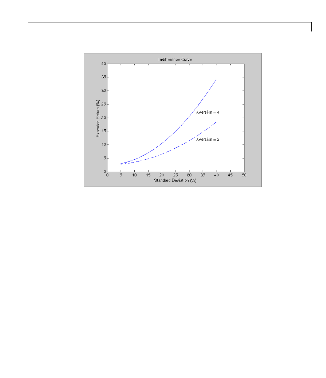
Portfolio Selection and Risk Aversion

Optimal Risky Portfolio Example

This example computes the optimal risky portfolio on the efficient frontier based upon the risk-free rate, the borrowing rate, and the investor’s degree of risk aversion. You do this with the function

First generate the efficient frontier data using either This example uses

portopt and the same asset data from the previous

example.

ExpReturn = [0.1 0.2 0.15 ];

ExpCovariance = [ 0.005 -0.010 0.004;

-0.010 0.040 -0.002;

0.004 -0.002 0.023];

This time consider 20 different points along the efficient frontier.

NumPorts = 20;

portalloc.

portopt or frontcon.

3-9

3 Portfolio Analysis

[PortRisk, PortReturn, PortWts] = por topt(ExpReturn,... ExpCovariance, NumPorts);

As with frontcon,callingportopt w hile specifying output arguments returns the corresponding vectors and arrays representing the risk, return, and weights for each of the portfolios along the efficient frontier. Use them as the first three input arguments to the function

portalloc.

Now find the optimal risky portfolio and the opt imal allocation of funds between the risky portfo lio and the risk-free asset, using these values for the risk-free rate, borrowing rate and investor’s degree of risk aversion.

RisklessRate = 0.08 BorrowRate = 0.12 RiskAversion = 3

Calling po rtalloc without specifying any output arguments gives a graph displaying the critical points.

portalloc (PortRisk, PortReturn, PortWts, RisklessRate,... BorrowRate, RiskAversion);

3-10

Portfolio Selection and Risk Aversion

Calling portalloc while specifying the output arguments returns the variance ( (

RiskyWts) allocated to the optimal risky portfolio. It also returns the fraction

(

RiskyFraction) of the complete portfolio allocated to the risky portfolio,

and the variance (

RiskyRisk), the ex pected return (RiskyR eturn), and the weights

OverallRisk) and expected return (OverallReturn)ofthe

optimal overall portfolio. The overall portfolio combines investments in the risk-free asset and in the risky portfolio. The actual proportion assigned to each of these two investments is determined b y the degree of risk aversion characterizing the investor.

[RiskyRisk, RiskyReturn, RiskyWts,RiskyFraction, OverallRisk,...

OverallReturn] = portalloc (PortRisk, PortReturn, PortWts,...

RisklessRate, BorrowRate, RiskAversion)

RiskyRisk = 0.1288

RiskyReturn = 0.1791

RiskyWts = 0.0057 0.587 9 0.4064

RiskyFraction = 1.1869

OverallRisk = 0.1529

OverallReturn = 0.1902

The value of RiskyFraction exceeds 1 (100%), implying that the risk tolerance specified allows borrowing money to invest in the risky portfolio, an d that no money will be invested in the risk-free asset. This borrowed capital is added to the original capital available for investment. In this example the customer will tolerate borrow ing 18.69% of the original capital amount.

3-11

3 Portfolio Analysis

Constraint Specification

In this section...

“Example” on page 3-12

“Linear Constraint Equations” on page 3 -14

“Specifying Additional Constraints” on page 3-17

Example

This example computes the efficient frontier of portfolios consisting of three different assets, INTC, XON, and RD, given a list of constraints. The expected returns for INTC, XON, and RD are respectiv ely as follows:

ExpReturn = [0.1 0.2 0.15 ];

The covariance matrix is

ExpCovariance = [ 0.005 -0.010 0.004;

-0.010 0.040 -0.002;

0.004 -0.002 0.023];

3-12

• Constraint 1

- Allow short selling up to 10% of the portfolio value in any asset, but limit

the inves tment in any one asset to 110% of the portfolio value.

• Constraint 2

- Consider two different sectors, technology and energy, with the following

table indicating the sector each asset belongs to .

Asset

Sector

Constrain the investment in the Energy sector to 80% of the portfolio value, and the investment in the Technology sector to 70%.

To solve this problem, use Consider eight different portfolios along the efficient frontier:

INTC XON

Technology

frontcon, passing in a list of asset constraints.

Energy Energy

Constraint Specification

NumPorts = 8;

To introduce the asset bounds constraints specified in Constraint 1, create the matrix

AssetBounds, where each column represents an

asset. The upper row represents the lower bounds, and the lower row represents the upper bounds.

AssetBounds = [-0.10, -0. 10, -0.10;

1.10, 1.10, 1.10];

Constraint 2 needs to be entered in two parts, the first part defining the groups, and the second part defining the constraints for each group. Given the information above, you can build a matrix of 1s and 0s indicating whether a specific asset belongs to a group. Each column represents an asset, and each row represents a group. This example has twogroups:thetechnologygroup,and the energy group. Create the matrix

Groups as follows.

Groups = [0 1 1;

1 0 0];

The GroupBounds matrix allows you to specify an upper and lower bound for each group. Each row in this matrix represents a group. The first column represents the minimum allocation, and the second column represents the maximum allocation to each group. Since the investment in the Energy sector is capped at 80% of the portfolio value, and the investment in the Technology sector is capped at 70%, create the

GroupBounds matrix using this information.

GroupBounds = [0 0.80;

0 0.70];

Now use frontcon to obtain the vectors and arrays representing the risk, return, and weights for each of the eight portfolioscomputedalong the efficient frontier.

[PortRisk, PortReturn, PortWts] = front con(ExpReturn,... ExpCovariance, NumPorts, [], AssetBounds, Groups, GroupBounds)

PortRisk =

3-13

3 Portfolio Analysis

0.0416

0.0499

0.0624

0.0767

0.0920

0.1100

0.1378

0.1716

PortReturn =

0.1279

0.1361

0.1442

0.1524

0.1605

0.1687

0.1768

0.1850

3-14

PortWts =

0.7000 0.2582 0.0418

0.6031 0.3244 0.0725

0.4864 0.3708 0.1428

0.3696 0.4172 0.2132

0.2529 0.4636 0.2835

0.2000 0.5738 0.2262

0.2000 0.7369 0.0631

0.2000 0.9000 -0.1000

The output data is represented row-wi se, where each portfolio’s risk, rate of return, and associated weight is identified as corresponding rows in the vectors and matrix.

Linear Constraint Equations

While fron tcon allows you to enter a fixed set of constraints related to minimum and maximum values for groups and individual assets, you often need to specify a larger and more general set of constraints when finding

Constraint Specification

the optimal risky portfolio. The function portopt addresses this need, by accepting a n arbitrary set of constraints as an input matrix.

The auxiliary function

portcons can be used to create the matrix of

constraints, with each row representing an inequality. These inequalities are of the type vector of asset allocations. The number of columns of the matrix length of the vector rows of the matrix

A*Wts' <= b,whereA is a matrix, b is a vector, and Wts is a row

A,andthe

Wts correspond to the number of assets. The number of

A, and the length of vector b correspond to the number

of constraints. This method allows you to specify any number of linear inequalities to the function

In actuality,

portcons is an entry point to a set of functions that generate

matrices for specific types of constraints.

portopt.

portcons allows you to specify all

the constraints data at once, while the specific portfolio constraint functions allow you to build the constraints incrementally. These constraint functions are

pcpval, pcalims, pcglims,andpcgcomp.

Consider an example to help understand how to specify constraints to

portopt

whilebypassingtheuseofportcons. This example requires specifying the minimum and maximum investment in various groups.

Maximum and Minimum Group Exposure

Group Minimum Exposure Maximum Exposure

North America

Europe

Latin America

Asia

0.30 0.75

0.10 0.55

0.20 0.50

0.50 0.50

Note that the minimum and maximum exposure in Asia is the same. This means that you require a fixed exposure for this g roup.

Also assume that the portfolio consists of three different funds. The correspondence between funds and groups is shown in the table below.

3-15

3 Portfolio Analysis

Group Membership

Group Fund 1 Fund 2 Fund 3

North America

Europe X

Latin America

Asia

Using the information in these two tables, build a mathematical representation of the constraints represented. Assume that the vector of weights representing the exposure of each asset in a portfolio is called

Wts=[W1W2W3].

Specifically

W1+W2

W2+W3

≥

≤

≥

≤

≥

≤

0.30

0.75

0.10

0.55

0.20

0.50

3-16

Since you need to represent the information in the form multiply equations 1, 3 and 5 by –1. Also turn equation 7 into a set of two inequalities: W2+W3 ≥ 0.50 and W2+W3 ≤ 0.50. (The intersection of these two inequalities is the equality itself.) Thus

-W1-W2

W1+W2

-W3

≤

A*Wts <= b,

-0.30

0.75

-0.10

Constraint Specification

-W1

-W2-W3

W2+W3

≤

Bringing these equations into matrix notation gives

A=[-1 -1 0;

110; 0 0 -1; 001;

-1 0 0; 100; 0 -1 -1; 011]

b = [-0.30;

0.75;

-0.10;

0.55;

-0.20;

0.50;

-0.50;

0.50]

0.55

-0.20

0.50

-0.50

0.50

Build the constraint matrix ConSet by concatenating the matrix A to the vector

ConSet = [A, b]

Specifying Additional Constraints

The ex ample above defined a constraints matrix that specified a set of typical scenarios. It defined groups of assets, specifie d upper and lower bounds for totalallocationineachofthesegroups, and it set the total allocation of one of thegroupstoafixedvalue. Constraints like these are common occurrences.

3-17

3 Portfolio Analysis

The function portcons was created to simplify the creation of the constraint matrix for these and other common portfolio requirements.

portcons takes

as input arguments a list of constra in t- spe c if ie r strings, followed by the data necessary to build the constraint specified by the strings.

Assume that you need to add more constraints to the previous example. Specifically, add a constraint indicating that the sum of weights in any portfolio should be equal to 1, and another set of constraints (one per asset) indicating that the weight for each asset must greater than 0. This translates into five more constraint rows: two for the new equality, and three indicating that each weight must be greater or equal to 0. The total number of inequalities in the example is now 13. Clearly, creating the constraint matrix can turn into a tedious task.

To create the new constraint matrix using

portcons, use two separate

constraint-specifier strings:

•

'Default', which indicates that each weight is greater than 0 and that the

total sum of the weights adds to 1

•

'GroupLims', which defines the minimum and maximum allocation on

each group

The only data requirement for the constraint-specifier string

'Default'

is NumAssets (the total number of assets). The constraint-specifier string

'GroupLims' requires three different arguments: a Groups matrix indicating

the assets that belong to each group, the minimum bounds for each group, and the

GroupMin vector indicating the

GroupMax vector indicating the

maximum bounds for each group. Based on the table Group Membership on page 3-16, build the

Group matrix, with each row representing a group, and

each column representing an asset.

Group = [1 1 0;

001; 100; 011]

The table Ma xim u m and Minimum Group Exposure on page 3-15 has the information to build

GroupMin and GroupMax.

3-18

GroupMin = [0.30 0.10 0.20 0.50];

Mathworks FINANCIAL TOOLBOX 3 user guide

Specifications and Main Features

Frequently Asked Questions

User Manual

Getting Started

Product Overview

Expected Background

Using Matrix F unctions for Finance

Introduction

Key Definitions

Referencing Matrix Elements

Transposing Matrices

Matrix Algebra Refresher

Introduction

Adding and Subtracting Matrices

Multiplying Matrices

Multiplying Vectors

Computing Dot Products of Vectors

Multiplying Vectors and Matrices

Multiplying Two Matrices

Multiplying a Matrix by a Scalar

Dividing Matrices

Solving Simultaneou s Linear Equations

Operating Element by Element

Function Input and Output Arguments

Input Arguments

Matrix Input

Matrices of String Input

Output Arguments

Interest Rate Arguments

Performing Common Financial Tasks

Introduction

Handling and Converting Dates

Date Formats

Date Conversions

Input Conversions

Output Conversions

CurrentDateandTime

Determining Dates

Formatting Currency

Charting Financial Data

Introduction

High-Low-Close Chart Example

Bollinger Chart Example

Analyzing and Computing Cash Flows

Introduction

Interest Rates/Rates of Return

Present or Future Values

Depreciation

Annuities

Pricing and Computing Yields for Fixed-Income Securities

Introduction

Terminology

Period of a Bond

Basis of a Bond

End-of-Month Rule

Framework

Common Input Arguments

Default Parameter Values

Single Bond Example

Bond Portfolio Example

Coupon Date Calculations

Yield Functions

Calculating Duration and Convexity for Bonds

Calculating Key Rate Durations for Bonds

Term Structure of Interest Rates

Introduction

Deriving an Implied Z ero Cur ve

Pricing and Analyzing Equity Derivatives

Introduction

Sensitivity Measures

Delta

Gamma

Lambda

Theta

Vega

Implied Volatility

Analysis Models

Black-Scholes Model

Binomial Model