Mathworks FINANCIAL DERIVATIVES TOOLBOX 5 user guide

Financial Derivat

User’s Guide

ives Toolbox™ 5

How to Contact The MathWorks

www.mathworks.
comp.soft-sys.matlab Newsgroup
www.mathworks.com/contact_TS.html Technical Support

[e-mail] Product enhancement suggestions

bugs@mathwo
[e-mail] Documentation error reports
[e-mail] Order status, license renewals, passcodes

info@mathwo

com

rks.com

rks.com

Web

Bug reports

Sales, prici

ng, and general information

508-647-7000 (Phone)

508-647-7001 (Fax)

The MathWorks, Inc.
3 Apple Hill Drive
Natick, MA 01760-2098

For contact information about worldwide offices, see the MathWorks Web site.

Financial Derivatives Toolbox™ User’s G uide

© COPY R IGHT 2000–2010 The MathW orks, Inc.

The software described in this document is furnished under a license agreement. The software may be used
or copied only under the terms of the license agreement. No part of this manual may be photocopied or
reproduced in any form without prior written consent from The MathW orks, Inc.

FEDERAL ACQUISITION: This provision applies to all acquisitions of the Program and Documentation
by, for, or through the federal government of the United States. By accepting delivery of the Program
or Documentation, the government hereby agrees that this s oftware or docume n tation qualifies as
commercial computer software or commercial computer software documentation as such terms are used
or defined in FAR 12.212, DFARS Part 227.72, and DFARS 252.227-7014. Accordingly, the terms and
conditions of this Agreement and only those rights specified in this Agreement, shall pertain to and govern
theuse,modification,reproduction,release,performance,display,anddisclosureoftheProgramand
Documentation by the federal government (or other entity acquiring for or through the federal government)
and shall supersede any conflicting contractual terms or conditions. If this License fails to meet the
government’s needs or is inconsistent in any respect with federal procurement law, the government agrees
to return the Program and Docu mentation, unused, to The MathWorks, Inc.

Trademarks

MATLAB and Simulink are registered trademarks of The MathWorks, Inc. See

www.mathworks.com/trademarks for a list of additional trademarks. Other product or brand

names may be trademarks or registered trademarks of their respective holders.

Patents

The MathWorks products are protected by one or more U.S. patents. Please see

www.mathworks.com/patents for more information.

Revision History

June 2000 First printing New for Version 1.0 (Release 12)
September 2001 Second printing Revised for Version 2.0 (Release 12.1)
April 2004 Third printing Revised for Version 3.0 (Release 14)
September 2005 Fourth printing Revised for Version 4.0 (Release 14SP3)
March 2006 Online only Revised for Version 4.0.1 (Release 2006a)
September 2006 Online only Revised for Version 4.1 (Release 2006b)
March 2007 Fifth printing Revised for Version 5.0 (Release 2007a)
September 2007 Sixth printing Revised for Version 5.1 (Release 2007b)
March 2008 Online only Revised for Version 5.2 (Release 2008a)
October 2008 Online only Revised for Version 5.3 (Release 2008b)
March 2009 Online only Revised for Version 5.4 (Release 2009a)
September 2009 Online only Revised for Version 5.5 (Release 2009b)
March 2010 Online only Revised for Version 5.5.1 (Release 2010a)

Getting Started

1

Product Overview ................................. 1-2

Introduction
Interest-Rate-Based Derivativ es
Equity-Based Derivatives

...................................... 1-2

..................... 1-2

........................... 1-3

Contents

Expected Background

Portfolio Creation

Introduction
Interest-Rate-Based Derivativ es
Equity Derivatives
Adding Instruments to an Existing Portfolio

Portfolio Management

Instrument Constructors
Creating New Instruments or Properties
Searching or Subsetting a Portfolio

...................................... 1-5

.............................. 1-4

................................. 1-5

................................ 1-6

............................. 1-9

........................... 1-9

Interest-Rate Derivatives

2

Understanding Interest-Rate Derivative

Instruments

Introduction
Bond
Bond Options
Bond with Embedded Options
Fixed-Rate Note
Floating-Rate Note
Cap
Floor

............................................ 2-3

............................................. 2-7

............................................ 2-7

..................................... 2-2

...................................... 2-2

..................................... 2-4

.................................. 2-5

................................ 2-6

..................... 1-5

........... 1-7

.............. 1-10

................... 1-12

....................... 2-5

v

Swap ............................................ 2-8

Swaption

........................................ 2-9

Overview of Interest-Rate Models

Interest-Rate Modeling
Rate and Price Trees
Viewing Rate or Price Movement with This Toolbox

Understanding the Interest-Rate Term Structure

Introduction
Interest Rates Versus Discount Factors
Interest-Rate Term Conversions
Functions That Model the Interest-Rate Term Structure

Computing Prices and Sensitivities Using the

Interest-Rate T erm Structure

Introduction
Computing Instrument Prices
Computing Instrument Sensitivities

Understanding Interest-Rate Tree Models

Introduction
Building a Tree of Forward Rates
Specifying the Volatility Model (VolSpec)
Specifying the Interest-Rate Term Structure (RateSpec)
Calibrating the Hull-White Model Using Market Data
Specifying the Time Structure (TimeSpec)
Examples of Tree Creation
Examining Trees

...................................... 2-15

...................................... 2-30

...................................... 2-35

............................. 2-10

............................... 2-11

.......................... 2-49

.................................. 2-50

................... 2-10

............... 2-15

..................... 2-20

..................... 2-30

....................... 2-31

.................. 2-33

........... 2-35

.................... 2-36

.............. 2-38

............. 2-47

..... 2-12

..... 2-15

.. 2-24

.. 2-41

... 2-42

vi Contents

Computing Prices and Sensitivities Using Interest-Rate

Tree Models

Introduction
Computing Instrument Prices
Computing Instrument Sensitivities

Interest-Rate Derivatives Using Closed Form

Solutions

Pricing C aps and Floors Using the Black Option Model

Graphical Representation of Trees

..................................... 2-62

...................................... 2-62

....................... 2-62

.................. 2-71

....................................... 2-74

.. 2-74

.................. 2-75

Introduction ...................................... 2-75

Observing Interest Rates
Observing Instrument Prices

........................... 2-75

........................ 2-79

Equity Derivatives

3

Understanding Equity Trees ........................ 3-2

Introduction
Building Equity Binary Trees
Building Implied Trinomial Trees
Examining Equity Trees
Differences Between CRR and EQP Tree Structures

...................................... 3-2

....................... 3-3

.................... 3-8

........................... 3-16

..... 3-20

Understanding Equity Exotic Options

Introduction
Asian Option
Barrier Option
Basket Option
Compound Option
Lookback Optio n
Digital Option
Rainbow Option
Vanilla Option

Computing Prices a n d Sensitivitie s for Equity

Derivatives Using Trees

Computing Instrument Prices
Computing Prices Using CRR
Computing Prices Using EQP
Computing Prices Using ITT
Examining Output from the Pricing Functions
Computing Instrument Sensitivities
Graphical Representation of CRR, EQP, and ITT Trees

Equity Derivatives Using Closed-Form Solutions

Introduction
Computing Prices and Sensitivities Using the Black-Scholes

Model

...................................... 3-22

..................................... 3-22

.................................... 3-23

.................................... 3-25

................................. 3-26

.................................. 3-27

.................................... 3-28

................................... 3-29

.................................... 3-30

.......................... 3-32

....................... 3-32

....................... 3-34

....................... 3-36

........................ 3-38

...................................... 3-50

......................................... 3-54

............... 3-22

.......... 3-40

.................. 3-44

.. 3-48

..... 3-50

vii

Computing Prices and Sensitivities Using the Black

Model

Computing Prices and Sensitivities Using the

Roll-Geske-Whaley Model

Computing Prices and Sensitivities Using the

Bjerksund-Stensland Model

......................................... 3-56

........................ 3-57

....................... 3-58

Hedging Portfolios

4

Hedging .......................................... 4-2

Hedging Function s

Introduction
Hedging with hedgeopt
Self-Financing Hedges with hedgeslf

Specifying Constraints with ConSet

Introduction
Setting Constraints
Portfolio Rebalancing

Hedging with Co n strained Portfolios

Overview
Example: Fully Hedged Portfolio
Example: Minimize Portfolio Sensitivities
Example: Under-Determined System
Example: Portfolio Constraints with hedgeslf

...................................... 4-3

...................................... 4-16

........................................ 4-21

................................ 4-3

............................. 4-4

................................ 4-16

.............................. 4-19

5

.................. 4-12

................. 4-16

................ 4-21

..................... 4-21

............. 4-24

................. 4-25

.......... 4-27

Function Reference

viii Contents

Portfolio Hedge Allocation ......................... 5-3

Interest-Rate T erm Structure

....................... 5-3

Heath-Jarrow-Morton Trees ........................ 5-3

Black-Derman-Toy Trees

Black-Karasinski Trees

Cox-Ross-Rubinstein Trees

Equal Probabilities Binomial Trees

Hull-White Trees

Implied Trinomial Tree

Heath-Jarrow-Morton Utilities

Black-Derman-Toy Utilities

Black-Karasinski Utilities

Cox-Ross-Rubinstein Utilities

.................................. 5-6

........................... 5-4

............................ 5-4

......................... 5-5

............................ 5-6

...................... 5-7

......................... 5-7

.......................... 5-8

....................... 5-9

................. 5-5

Equal Probabilities Tree Utilities

Implied Trinomial Tree Utilities

Hull-White Utilities

Tree Manipulation

Derivatives Pricing Options

Pricing and Sensitivity Using Black-Scholes Option

Pricing Model

................................ 5-11

................................. 5-11

................................... 5-12

................... 5-10

.................... 5-10

........................ 5-12

ix

Pricing and Sensitivity Using Black Option Pricing

Model

Pricing and Sensitivity Using Longstaff-Schwartz

Option Pricing Model

Pricing and Sensitivity Using Nengjiu Ju

Approximation Model

Pricing and Sensitivity Using Role-Geske-Whaley

Option Pricing Model

Pricing and Sensitivity Using Bjerksund-Stensland

Option Pricing Model

Pricing and Sensitivity Using Stulz Option Pricing

Model

.......................................... 5-13

............................ 5-14

............................ 5-14

............................ 5-15

............................ 5-15

.......................................... 5-16

Instrument Portfolio Handling

Financial Object Structures

Interest Term Structure

Date

Graphical Display

.............................................. 5-18

............................ 5-18

................................. 5-19

...................... 5-16

........................ 5-18

x Contents

Functions — Alphabetical List

6

Derivatives Pricing Options

A

Pricing Options Structure .......................... A-2

Introduction
Default Structure

...................................... A-2

................................. A-2

Customizing the Structure

......................... A-5

Bibliography

B

Black-Derman-Toy (BDT) Modeling ................. B-2

Heath-Jarrow-Morton (HJM) Modeling

Hull-White (HW) and Bla ck-Karasinski (BK)

Modeling

Cox-Ross-Rubinstein (CRR) Modeling

Implied Trinomial Tree (ITT) Modeling

Equal Probabilities Tree (EQP) Modeling

....................................... B-4

.............. B-3

............... B-5

.............. B-6

............ B-7

Closed-Form Solutions Modeling

Financial Derivatives

.............................. B-9

.................... B-8

xi

Examples

C

Instrument Portfolio Examples ..................... C-2

Interest Rate Environment Examples

HJM Examples

Volatility Modeling

BDT Examples

Rate Specification Creation

Time Specification

Sensitivity

Treeviewer Examples

Creating Equity Derivatives

Pricing Equity Derivatives

.................................... C-2

................................ C-2

..................................... C-2

........................ C-3

................................. C-3

........................................ C-3

.............................. C-3

........................ C-3

......................... C-4

............... C-2

xii Contents

Closed-Form Solution Examples

Hedging Examples

Hedging with Co n strained Portfolios

................................. C-4

.................... C-4

................ C-4

Glossary

Index

xiii

xiv Contents

Getting Started

• “Product Overview” on page 1-2

• “Expected Background” on p age 1-4

• “Portfolio Creation” on p age 1-5

• “Portfolio Management” on page 1-9

1

1 Getting Started

Product Overview

Introduction

Financial D erivative s Toolbox™ software provides components for analyzing
individual derivative instruments and portfolios containing several types of
interest-rate-based and equity-based financial instruments.

Interest-Rate-Based Derivatives

The toolbox provides functionality that supports the creation and management
of these interest-rate-based instruments:

In this section...

“Introduction” on page 1-2

“Interest-Rate-Based Derivatives” on page 1-2

“Equity-Based Derivatives” on page 1-3

1-2

• Bonds

• Bond options (puts and calls)

• Caps

• Fixed-rate notes

• Floating-rate notes

• Floors

• Swaps

• Swaption

• CallableandPuttablebonds

Additionally, the toolbox provides functions to create arbitrary cash flow
instruments. The toolbox provides pricing and sensitivity routines for these

instruments. See “Computing Prices and Sensitivities Using the Interest-Rate
Term Structure” on page 2-30 or “Computing Prices and Sensitivities Using
Interest-Rate Tree Models” on pag e 2-62 for information.

Product Overview

Equity-Based De

The toolbox also
derivatives, in

• Asian option s

• Barrier optio

• Compound opti

• Lookback opt

• Vanilla stoc

The toolbox
instrument
Using Tree

provides functions to create and manage various equity-based

cluding the following:

ns

ons

ions

k options (put and call options)

also provides pricing and sensitivity routines for these
s. (See “Computing Prices and Sensitivities for Equity Derivatives
s” on page 3-32.)

rivatives

1-3

1 Getting Started

Expected Background

In general, this guide assumes experience working with financial derivatives
and some familiarity with the underlying models.

In designing Financial Derivatives Toolbox documentation, we assume your
title is similar to one of these:

• Analyst, quantitative analyst

• Risk manager

• Portfolio manager

• Fund manager, asset m anager

• Financial engineer

• Trader

• Student, professor, or other academic

1-4

We also assum e your background, education, training, and responsibilities
match some aspects of this profile:

• Finance, economics, perhaps accounting

• Engineering, mathematics, physics, other quantitative sciences

• Bachelor’s degree minimum; MS or MBA likely; Ph.D. perhaps; CFA

• Comfortable with probability theory, statistics, and algebra

• Understand linear or m atrix algebra, calculus, and differential equations

• Previously done traditional programming(C,Fortran,etc.)

• Responsible for instruments or analyses involving large sums of money

• Perhaps new to MATLAB

Portfolio Creation

In this section...

“Introduction” on page 1-5

“Interest-Rate-Based Derivatives” on page 1-5

“Equity Derivatives” on page 1-6

“Adding Instruments to an Existing Portfolio” on page 1-7

Introduction

The instadd function creates a set of instruments (portfolio) or adds
instruments to an existing instrument collection. The
specifies the type of the investment instrument. For interest-rate-based
derivatives, the types are:

Floor,andSwap. For equity derivatives, the types are Asian, Barrier,
Compound, Lookback,andOptStock.

Portfolio Creation

TypeString argument

Bond, OptBond, CashFlow, Fixed, Float, Cap,

The input arguments following
investment instrument. Thus, the
remainder of the input arguments is interpreted. For example,
thetypestring

InstSet = instadd('Bond', CouponRate, Settle, Maturity, Period,
Basis, EndMonthRule, IssueDate, FirstCouponDate, LastCouponDate,
StartDate, Face)

Bond creates a portfolio of bond instruments.

TypeString are specific to the type of

TypeString argument determines how the

instadd with

Interest-Rate-Based Derivatives

In addition to the bond instrument already described, the toolbox can create
portfolios containing the following set of interest-rate-based derivatives:

• Bond option

InstSet = instadd('OptBond', BondIndex, OptSpec, Strike, ExerciseDates, AmericanOpt)

• Arbitrary cash flow instrument

InstSet = instadd('CashFlow', CFlowAmounts, CFlowDates, Settle, Basis)

1-5

1 Getting Started

• Fixed-rate note instrument

InstSet = instadd('Fixed', CouponRate, Settle, Maturity, FixedReset, Basis, Principal)

• Floating-rate note instrument

InstSet = instadd('Float', Spread, Settle, Maturity, FloatReset, Basis, Principal)

• Cap instrument

InstSet = instadd('Cap', Strike, Settle, Maturity, CapReset, Basis, Principal)

• Floor instrument

InstSet = instadd('Floor', Strike, Settle, Maturity, FloorReset, Basis, Principal)

• Swap instrument

InstSet = instadd('Swap', LegRate, Settle, Maturity, LegReset, Basis, Principal, LegType)

• Swaption instrument

1-6

InstSet = instadd('Swaption', OptSpec, Strike, ExerciseDates, Spread, ...

Settle, Maturity, AmericanOpt, SwapReset, Basis, Principal)

• Bond with embedded option instrument

InstSet = instadd('OptEmBond', CouponRate, Settle, Maturity, OptSpec, Strike, ...

ExerciseDates, 'AmericanOpt', AmericanOpt, 'Period', Period,'Basis', Basis, ...

'EndMonthRule', EndMonthRule,'Face',Face,'IssueDate', IssueDate, 'FirstCouponDate', ...

FirstCouponDate, 'LastCouponDate', LastCouponDate,'StartDate', StartDate)

Equity Derivatives

The toolbox can create portfolios con taining the following set of equity
derivatives:

• Asian instrument

InstSet = instadd('Asian', OptSpec, Strike, Settle, ExerciseDates, AmericanOpt, ...

AvgType, AvgPrice, AvgDate)

• Barrier instrument

Portfolio Creation

InstSet = instadd('Barrier', OptSpec, Strike, Settle, ExerciseDates, AmericanOpt, ...

BarrierType, Barrier, Rebate)

• Compound instrument

InstSet = instadd('Compound', UOptSpec, UStrike, USettle, UExerciseDates, UAmericanOpt, ...

COptSpec, CStrike, CSettle, CExerciseDates, CAmericanOpt)

• Lookback instrument

InstSet = instadd('Lookback', OptSpec, Strike, Settle, ExerciseDates, AmericanOpt)

• Stock option instrument

InstSet = instadd('OptStock', OptSpec, Strike, Settle, Maturity, AmericanOpt)

Adding Instruments to an Existing Portfolio

To use the instadd function to add additional instruments to an existing
instrument portfolio, provide the name of an existing portfolio as the first
argument to the

instadd function.

Consider, for example, a portfolio containing two cap instruments only:

Strike = [0.06; 0.07];
Settle = '08-Feb-2000';
Maturity = '15-Jan-2003';

Port_1 = instadd('Cap', Strike, Settle, Maturity);

These commands create a portfolio containing two cap instruments with the
same settlement and maturity dates, but with different strikes. In general,
the input arguments describing an instrument can be either a scalar, or
a number of instruments (

NumInst)-by-1 vector in which each element

corresponds to an instrument. Using a scalar assigns the same value to all
instruments passed in the call to

Use the

instdisp command to display the contents of the instrument set:

instdisp(Port_1)

Index Type Strike Settl e Maturity CapReset Basis Principal

instadd.

1-7

1 Getting Started

1 Cap 0.06 08-Feb-2000 15-Jan-2003 1 0 100

2 Cap 0.07 08-Feb-2000 15-Jan-2003 1 0 100

Now add a single bond instrument to Port_1. The bond has a 4.0% coupon
and the same settlement and maturity dates as the cap instruments.

CouponRate = 0.04;

Port_1 = instadd(Port_1, 'Bond', CouponRate, Settle, Maturity);

Use in stdi sp again to see the resulting instrument set:

instdisp(Port_1)

Index Type Strike Settle Maturity CapReset Basis Principal

1 Cap 0.06 08-Feb-2000 15-Jan-2003 1 0 100

2 Cap 0.07 08-Feb-2000 15-Jan-2003 1 0 100

Index Type CouponRate Settle Maturity Period Basis EndMonthRule IssueDate ... Face

3 Bond 0.04 08-Feb-2000 15-Jan-2003 2 0 1 NaN ... 100

1-8

Portfolio Management

In this section...

“Instrument Constructors” on page 1-9

“Creating New Instruments or Properties” on page 1-10

“Searching or Subsetting a Portfolio” on page 1-12

Instrument Constructors

The toolbox provides constructors for the most common financial instruments.
A constructor is a function that builds a structure dedicated to a certain type
of object; in this toolbox, an object is a type of market instrument.

The instruments and their constructors in this toolbox are listed below.

Instrument Constructor

Asian option

Barrier option

Bond

Bond option

Arbitrary cash flow

Compound option

Fixed-rate note

Floating-rate note

Cap

Floor

Lookback option

Stock option

Swap

Swaption

Portfolio Management

instasian

instbarrier

instbond

instoptbnd

instcf

instcompound

instfixed

instfloat

instcap

instfloor

instlookback

instoptstock

instswap

instswaption

1-9

1 Getting Started

Each instrument has parameters (fields) that describe the instrument. The
toolbox functions let you do the following:

• Create an instrum ent or portfolio of instruments.

• Enumerate stored instrument types and infor mation fields.

• Enumerate instrument field data.

• Search and select instruments.

The instrument structure consists of various fields according to instrument
type. A field is an element of data associated with the instrument. For
example, a bond instrument contains the fields

Maturity,andsoon. Additionally,eachinstrument has a field that identifies

the investment type (bond, cap, floor, and so on).

In reality, the set of parameters for each instrument is not fixed. You have
the ability to add additional parameters. These additional fields are ignored
by the toolbox functions. They may be used to attach additional information
to each instrument, such as a n internal code describing the bond.

CouponRate, Settle,

1-10

Parameters not specified when creating an instrument default to
in general, means that the functions using the instrument set (such as

intenvprice or hjmprice ) will use default values. At the time of pricing,

an error occurs if any of the required fields is missing, such as
cap or

CouponRate in a bon d.

NaN,which,

Strike in a

Creating New Instruments or Properties

Use the instaddfield function to create a kind of instrument or to add new
properties to the i ns trume n ts in an existing instrument col le ction.

To create a kind of instrument with
arguments:

•

Type

• FieldName

• Data

instaddfield, you must specify three

Portfolio Management

Type defines the type of the new instrument, for example, Future. FieldName

names the fields uniquely associated with the new type of instrument. Data
contains the data for the fields of the new instrument.

An optional fourth argument is

ClassList. ClassList specifies the da ta

types of the contents of each unique field for the new instrument.

Use either syntax to create a kind of instrument using

InstSet = instaddfield('FieldName', FieldList, 'Data', DataList,...

'Type', TypeString)

InstSet = instaddfield('FieldName', FieldList, 'FieldClass',...

ClassList, 'Data' , Dat aList, 'Type', TypeString)

instaddfield:

To add new instruments to an existing set, use:

InstSetNew = instaddfield(InstSetOld, 'FieldName', FieldList,...

'Data', DataList, 'Type', TypeString)

As an example, consider a futures contract with a delivery date of July 1 5,
2000, and a quoted price of $104.40. Since Financial Derivatives Toolbox
software does not directly support this instrument, you must create it using
the function

• Type:

instaddfield. Use these parameters to create instruments:

Future

• Field names: Delivery and Price

• Data: Delivery is July 15, 2000, and price is $104.40.

Enter the data into MATLAB

®

software:

Type = 'Future';
FieldName = {'Delivery', 'Price'};
Data = {'Jul-15-2000', 104.4};

Finally, create the portfolio with a single instrument:

Port = instaddfield('Type', Type, 'FieldName', FieldName,...
'Data', Data);

1-11

1 Getting Started

Now use the function instdisp to examine the resulting single-instrument
portfolio:

instdisp(Port)

Index Type Delivery Price
1 Future Jul-15-2000 104.4

Because your portfolio Port has the same structure as those created using
the function
portfolios created using
cap instruments to

Strike = [0.06; 0.07];

Settle = '08-Feb-2000';

Maturity = '15-Jan-2003';

Port = instadd(Port, 'C ap', Strike, Settle, Maturity);

instadd, y ou can combine portfolios created using instadd with

instaddfield. For example, you can now add two

Port with instadd.

View the resulting portfolio using instdisp.

1-12

instdisp(Port)

Index Type Delivery Price

1 Future 15-Jul-2000 104.4

Index Type Strike Settl e Maturity CapReset Basis Principal

2 Cap 0.06 08-Feb-2000 15-Jan-2003 1 0 100

3 Cap 0.07 08-Feb-2000 15-Jan-2003 1 0 100

Searching or Subsetting a Por tfolio

Financial Derivatives Toolbox software provides functions that enable y ou to:

• Find specific instruments within a portfolio.

• Create a subse t portfolio consisting of instruments selected from a larger

portfolio.

The

instfind function finds instruments with a specific parameter value;

it returns an instrument index (position) in a large instrument set. The

instselect function, on the other hand, subsets a large instrument set into

Portfolio Management

a portfolio of instruments w ith designated parameter values; it returns an
instrument set (portfolio) rather than an index.

instfind

The general syntax for instfind is

IndexMatch = instfind(InstSet, 'FieldName', FieldList, 'Data',...

DataList, 'Index', IndexSet, 'Type', TypeList)

InstSet is the instrument set to search. Within InstSet instruments

categorized by type, each type can have different da ta fields. T he stored data
field is a row vector or string for each instrument.

The

FieldList, DataList,andTypeList arguments indicate v alues to

search for in the
set.

FieldList is a cell array of field name(s) specific to the instruments.

DataList is a cell array or matrix of acceptable values for the parameter(s)

specified in

DataList) parameters must appear tog ether or not at all.

FieldName, Data,andType data fields of the instrument

FieldList. FieldName and Data (consequently, Field List and

IndexSet is a vector of integer index(es) designating positions of instruments

in the instrument set to check for matches; the default is all indices available
in the instrument set.
instruments to match one of the

TypeList is a string or cell array of strings restricting

TypeList types; the default is all types in the

instrument set.

IndexMatch is a vector of positions of instruments matching the input

criteria. Instruments are returned in

Index,andType conditions are met. An instrument meets an individual

field condition if the stored
in the

DataList for that FieldName.

FieldName data matches any of the rows listed

instfind Examples. TheexamplesusetheprovidedMAT-file

The MAT-file contains an instrument set,

IndexMatch if all the FieldName, Data,

deriv.mat.

HJMInstSet, that contains eight

instruments of sev en types.

1-13

1 Getting Started

load deriv.mat

instdisp(HJMInstSet)

Index Type CouponRate Settle Maturity Period Basis ... Name Quantity

1 Bond 0.04 01-Jan-2000 01-Jan-2003 1 NaN ... 4% bond 100

2 Bond 0.04 01-Jan-2000 01-Jan-2004 2 NaN ... 4% bond 50

Index Type UnderInd OptSpec Strike ExerciseDates AmericanOpt Name Quantity

3 OptBond 2 call 101 01-Jan-2003 NaN Option 101 -50

Index Type CouponRate Settle Maturity FixedReset Basis Principal Name Quantity

4 Fixed 0.04 01-Jan-2000 01-Jan-2003 1 NaN NaN 4% Fixed 80

Index Type Spread Settle Maturity FloatReset Basis Principal Name Quantity

5 Float 20 01-Jan-2000 01-Jan-2003 1 NaN NaN 20BP Float 8

Index Type Strike Settle Maturity CapReset Basis Principal Name Quantity

6 Cap 0.03 01-Jan-2000 01-Jan-2004 1 NaN NaN 3% Cap 30

1-14

Index Type Strike Settle Maturity FloorReset Basis Principal Name Quantity

7 Floor 0.03 01-Jan-2000 01-Jan-2004 1 NaN NaN 3% Floor 40

Index Type LegRate Settle Maturity LegReset Basis Principal LegType Name Quantity

8 Swap [0.06 20] 01-Jan-2000 01-Jan-2003 [1 1] NaN NaN [NaN] 6%/20BP Swap 10

Find all instruments with a maturity date of January 01, 2003.

Mat2003 = ...
instfind(HJMInstSet,'FieldName','Maturity','Data','01-Jan-2003')

Mat2003 =

1
4
5
8

Find all cap and floor instruments with a maturity date of January 01, 2004.

Portfolio Management

CapFloor = instfind(HJMInstSet,...
'FieldName','Maturity','Data','01-Jan-2004', 'Type',...
{'Cap';'Floor'})

CapFloor =

6
7

Find all instruments where the portfolio is long or short a quantity of 50.

Pos50 = instfind(HJMInstSet,'FieldName',...
'Quantity','Data',{'50';'-50'})

Pos50 =

2
3

instselect

The syntax for instselect is the same syntax as for instfind. ins tsel ect
returns a full portfolio instead of indexes into the original portfolio. Compare
the values returned by both functions by calling them equivalently.

Previously you used
maturity date of January 01, 2003.

Mat2003 = ...
instfind(HJMInstSet,'FieldName','Maturity','Data','01-Jan-2003')

Mat2003 =

1
4
5
8

Now use the same instrument set as a starting point, but execute the

instselect function instead, to produce a new instrument set matching

the identical search criteria.

instfind to find all instruments in HJMInstSet with a

1-15

1 Getting Started

Index Type CouponRate Settle Maturity Period Basis ......... Name Quantity

1 Bond 0.04 01-Jan-2000 01-Jan-2003 1 NaN ......... 4% bond 100

Index Type CouponRate Settle Maturity FixedReset Basis Principal Name Quantity

2 Fixed 0.04 01-Jan-2000 01-Jan-2003 1 NaN NaN 4% Fixed 80

Index Type Spread Settle Maturity FloatReset Basis Principal Name Quantity

3 Float 20 01-Jan-2000 01-Jan-2003 1 NaN NaN 20BP Float 8

Index Type LegRate Settle Maturity LegReset Basis Principal LegType Name Quantity

4 Swap [0.06 20] 01-Jan-2000 01-Jan-2003 [1 1] NaN NaN [NaN] 6%/20BP Swap 10

Select2003 = ...
instselect(HJMInstSet,'FieldName','Maturity','Data',...
'01-Jan-2003')

instdisp(Select2003)

1-16

instselect Examples. These examples use the portfolio ExampleInst
provided with the MAT-file InstSetExamples.mat.

load InstSetExamples.mat
instdisp(ExampleInst)

Index Type Strike Price Opt Contracts
1 Option 95 12.2 Call 0
2 Option 100 9.2 Call 0
3 Option 105 6.8 Call 1000

Index Type Delivery F Contracts
4 Futures 01-Jul-1999 104.4 -1000

Index Type Strike Price Opt Contracts
5 Option 105 7.4 Put -1000
6 Option 95 2.9 Put 0

Index Type Price Maturity Contracts
7 TBill 99 01-Jul-1999 6

Portfolio Management

The instrument set contains 3 instrument types: Option, Futures,andTBill.
Use

instselect to make a new instrument set containing only options struck

at

95. In other words, select all instruments containing the field Strike and

with the data value for that field equal to

InstSet = instselect(ExampleInst,'FieldName','Str ike','Data',95);

instdisp(InstSet)

Index Type Strike Price Opt Contracts

1 Option 95 12.2 Call 0

2 Option 95 2.9 Put 0

95.

You can use all the various forms of instselect and instfind to locate
specific instruments within this instrument set.

1-17

1 Getting Started

1-18

Interest-Rate Derivatives

• “Understanding Interest-Rate Derivative Instruments” on page 2-2

• “Overview of Interest-Rate Models” on page 2-10

• “Understanding the Interest-Rate Term Structure” on page 2-15

• “Computing Prices and Sensitivities Using the Interest-Rate Term

Structure” on page 2-30

• “Understanding Interest-Rate Tree Models” on page 2-35

• “Computing Prices and Sensitiv ities Using Interest-Rate Tree M odels”

on page 2-62

2

• “Interest-Rate Derivatives Using Closed Form Solutions” on page 2-74

• “Graphical Representation of Trees” on page 2-75

2 Interest-Rate Derivatives

Understanding Interest-Rate Derivative Instruments

In this section...

“Introduction” on page 2-2

“Bond” on page 2-3

“Bond Options” on page 2-4

“Bond with Embedded Options” on page 2-5

“Fixed-Rate Note” on page 2-5

“Floating-Rate Note” on page 2-6

“Cap” on page 2-7

“Floor” on page 2 -7

“Swap” on page 2-8

“Swaption” on page 2-9

2-2

Introduction

Financial Derivatives Toolbox software extends the Financial Toolbox™
capabilities in the areas of fixed-income derivatives and securities contingent
on interest rates. The toolbox provides components for analyzing individual
financial derivative instruments and portfolios. Specifically, it provides
functions for calculating prices and sensitivities, for hedging, and for
visualizing results.

The toolbox provides a set of functions that perform computations on portfolios
containing the following interest-rate based financial instruments:

• Bond

• Bond options

• Bond with embedded options

• Fixed-rate note

• Floating-rate note

• Cap

Understanding Interest-Rate Derivative Instruments

• Floor

• Swap

• Swaption

Additionally, Financial Derivatives Toolbox software lets you create and
price arbitrary cash flow instruments based on zero-coupon bonds or on any
supported interest-rate model. For more information, see “Interest-Rate
Modeling” on page 2-10.

Bond

A bond is a long-term debt security with a preset interest-rate and maturity.
At maturity you must pay the principal and interest.

The price or value of a bond is determined by discounting the expected cash
flows of the bond to the present, u sing the appropriate discount rate. The
following equation represents the relationship of the expected cash flows
and discount rate:

t

2

⎡

⎛

11

−+

⎢

⎜

C

⎝

B

⎢

0

=

⎢

2

⎢
⎢

⎣

−

⎤

r

⎞

⎥

⎟

2

⎠

r

2

⎥
⎥
⎥

⎥

⎦

F

+

⎛

1

⎜
⎝

t

2

r

⎞

+

⎟

2

⎠

where:

B

is the bond value.

0

C is the annual coupon payment.

F isthefacevalueofthebond.

r is the required return on the bond.

t is the number o f years remaining until maturity.

Financial Derivatives Tool box supports the following for pric ing and
specifying a bond.

2-3

2 Interest-Rate Derivatives

Function Purpose

bondbybdt

bondbyhw

bondbybk

bondbyhjm

bondbyzero

instbond

Price a bond using a BDT interest-rate tree.

Price a bond using an HW interest-rate tree.

Price a bond using a BK interest-rate tree.

Price a bond using an HJM interest-rate tree.

Price a bond using a set of zero curves.

Construct a bond instrument.

Bond Options

Financial Derivatives Toolbox software supports three types of put and call
options on bonds:

• American option: An option that you exercise any time u ntil i ts expiration

date.

2-4

• European option: An option that you exercise only on its expiration date.

• Bermuda option: A Bermuda option resembles a hybrid of American and

European options. You can exercise it on predetermined dates only, usually
monthly.

Financial Derivatives Tool box supports the following for pric ing and
specifying a bond option.

Function Purpose

optbndbybdt

Price a bond option price using a BDT
interest-rate tree.

optbndbyhw

Price a bond option price u sin g an HW
interest-rate tree.

optbndbybk

Price a bond option price using a BK
interest-rate tree.

optbndbyhjm

Price a bond option price us ing an HJM
interest-rate tree.

instoptbnd

Construct a bond option instrument.

Understanding Interest-Rate Derivative Instruments

Bond with Embedd

A bond with embed
bond at a predete
Toolbox softwa
puttable bonds

The pricing fo

• For a callabl

• For a puttab

Financial
specifyin

Function Purpose

optembndbybdt

optembndbyhw

optem

optembndbyhjm

instoptembnd

Derivatives Toolbox supports the following for pricing and

g a bond with embedded options.

bndbybk

ded options allows the issuer to buy back or redeem the

rmined price at specified future dates. Financial Derivatives
re supports American, European, and Bermuda callable and
.

r a bond with embedded options is as follows:

ebond:

le bond:

ed Options

PriceCallableBond = BondPrice - BondCallOption

PricePuttableBond = PriceBond + PricePutOption

Price a bond with emb edded options using a
BDT interest-rate tree .

Price a
HW inte

Price a bond with emb edded options using a
BK interest-rate tree.

Price a bond with embedded options using an
HJM interest-rate tree.

Construct a bond-with-embedded-options
instrument.

bond with embedded options using an

rest rate tree.

xed-Rate Note

Fi

ixed-rate note is a long-term debt security with a preset interest rate

A f

nd. At maturity the interest must be paid. The principal may or may not

a

e paid at maturity. In Financial Derivatives Toolbox software, the principal

b

salwayspaidatmaturity.

i

Financial Derivatives Tool box supports the following for pric ing and
specifying a fixed-rate note.

2-5

2 Interest-Rate Derivatives

Function Purpose

fixedbybdt

Price a fixed-rate note using a BDT
interest-rate tree.

fixedbyhw

Price a fixed-rate note using an HW
interest-rate tree.

fixedbybk

Price a fixed-rate note us in g a BK interest-rate
tree.

fixedbyhjm

Price a fixed-rate note using an HJM
interest-rate tree.

fixedbyzero

Price a fixed-rate note using a set of zero
curves.

instfixed

Construct a fixed-rate instrument.

Floating-Rate Note

A floating-rate note is a security like a bond, but the interest rate of the note
is reset periodically, relative to a reference index rate, to reflect fluctuations
in market interest rates.

2-6

Financial Derivatives Tool box supports the following for pric ing and
specifying a floating-rate note.

Function Purpose

floatbybdt

Priceafloating-ratenoteusingaBDT
interest-rate tree.

floatbyhw

Priceafloating-ratenoteusinganHW
interest-rate tree.

floatbybk

Price a floating-rate note using a BK
interest-rate tree.

floatbyhjm

Priceafloating-ratenoteusinganHJM
interest-rate tree.

floatbyzero

Price a floating-rate note using a set of zero
curves.

instfloat

Construct a floating-rate note instrument.

Cap

A cap is a contrac
rate to be paid by
The payoff for a

max( , )CurrentRate CapRate− 0

t that includes a guarantee that sets the maximum interest

the holder, based on an otherwise floating interest rate.

cap is:

Understanding Interest-Rate Derivative Instruments

Financial De
specifying a

Function Purpose

capbybdt

capbyhw

capbybk

capbyhjm

capbyblk

cap

inst

rivatives Toolbox supports the following for pricing and

cap instrument.

Price a cap instrument using a BDT
interest-rate tree.

Price a ca
interest

Price a cap instrument using a BK interest-rate
tree.

Price a cap instrument using an HJM
interest-rate tree.

Price
pric

Cons

p instrument using an HW

-rate tree.

a cap instrument using the Black option

ing model.

truct a cap instrument.

Floor

A floor isacontractthatincludesaguarantee setting the minimum interest
rate to be received by the holder, basedonanotherwisefloatinginterest
rate. T he payoff for a floor is:

max( , )FloorRate CurrentRate− 0

Financial Derivatives Tool box supports the following for pric ing and
specifying a floor instrument.

2-7

2 Interest-Rate Derivatives

Function Purpose

floorbybdt

Price a floor instrument using a BDT
interest-rate tree.

floorbyhw

Price a floor instrument using an HW
interest-rate tree.

floorbybk

Price a floor instrument using a BK
interest-rate tree.

floorbyhjm

Price a floor instrument using an HJM
interest-rate tree.

instfloor

Construct a floor instrument.

Swap

A swap is contract between two parties obligating the parties to exchange
future cash flows. This toolbox version handles only the vanilla swap, which
is composed of a floating-rate leg and a fixed-rate leg.

2-8

Financial Derivatives Tool box supports the following for pric ing and
specifying a swap instrument.

Function Purpose

swapbybdt

Price a swap instrument using a BDT
interest-rate tree.

swapbyhw

Price a swap instrument usi n g an HW
interest-rate tree.

swapbybk

Price a swap instrument using a BK
interest-rate tree.

swapbyhjm

Price a swap instrument using an HJM
interest-rate tree.

swapbyzero

Price a swap instrument using a set of zero
curves.

instswap

Construct a swap instrument.

Understanding Interest-Rate Derivative Instruments

Swaption

A swaption is an option to enter into an interest-rate swap contract. A call
swaption allows the option buyer to enter into an interest-rate swap where the
buyer of the option pays the fixed-rate and receives the floating-rate. A put
swaption allows the option buyer to enter into an interest-rate swap w here
the buyer of the option receives the fixed-rate and pays the floating-rate.

Financial Derivatives Tool box supports the following for pric ing and
specifying a swaption instrument.

Function Purpose

swaptionby

swaptionbyhw

swaptionbybk

swapti

instswaption

bdt

onbyhjm

Price a swaption instrument using a BDT
interest-rate tree.

Price a swaption instrument using an HW
interest-rate tree.

Price a sw
interes

aption instrument using a BK

t-rate tree.

Price a swaption instrument using an H JM
interest-rate tree.

Construct a swaption instrument.

2-9

2 Interest-Rate Derivatives

Overview of Interest-Rate Models

In this section...

“Interest-Rate Modeling” on page 2-10

“Rate and Price Trees” on page 2-11

“Viewing Rate or Price Movement with This Toolbox” on page 2-12

Interest-Rate Modeling

Financial Derivatives Toolbox software computes prices and sensitivities of
interest-rate contingent claims based on several methods of modeling changes
in interest rates over time:

• The interest-rate term structure

Thismodelusessetsofzero-couponbonds to predict changes in interest
rates.

2-10

• Heath-Jarrow-Morton (HJM) model

The HJM model considers a given initial term structure of interest
rates and a specification of the volatility of forward rates to build a tree
representing the evolution of the interest rates, based on a statistical
process.

• Black-Derman-Toy (BDT) model

In the BDT model, all security prices and rates depend on the short rate
(annualized 1-period interest rate). The model uses long rates and their
volatilities to construct a tree of possiblefutureshortrates. Theresulting
tree can then be used to determine the v alue of interest-rate sensitive
securities from this tree.

• Hull-White (HW) model

The Hull-White model incorporates the initial term s tructure of interest
rates and the volatility term structure to build a trinomial recombining tree
of short rates. The resulting tree is used to value interest-rate d ependent
securities. The implementation of the HW model in Financial Derivatives
Toolbox software is limited to one factor.

• Black-Karasinski (BK) model

Overview of Interest-Rate Models

The BK model is a sing le-factor, log-normal version of the HW model.

For detailed information about interest-rate models, see:

• “Computing Prices and Sensitivities Using the Interest-Rate Term

Structure” on page 2-30 for a discussion of price a nd sensitivity based on
portfolios of ze ro-coupo n bonds

• “Computing Prices and Sensitivities Using Interest-Rate Tree Models” on

page 2-62 for a discussion of price and sensitivity based on the HJM and
BDT interest-rate models

Note Historically, the initial version of Financial Derivatives Toolbox
software provided only the HJM interest-rate model. A later version added
the BDT model. The current versionaddsboththeHWandBKmodels.
This chapter provides extensive examples of using the HJM and BDT
models to compute prices and sensitivities of interest-rate based financial
derivatives.

The HW and BK tree structures are similar to the BDT tree structure.
To avoid needless repetition throughout this chapter, documentation is
provided only where significant deviations from the BDT structure exist.
Specifically, “HW and BK Tree Structures” on page 2-57 explains the few
noteworthy differences among the various formats.

If you need more detailed information about functions that use the HW and
BK tree structures, see Chapter 5, “Function Reference”, which provides
extensive reference information for all functions that compose this toolbox.

Rate and Price Trees

The interest-rate or price trees supported in this toolbox can be either
binomial (two branches per node) or trinomial (3 branches per node).
Typically, binomial trees assume that u nderlying interest rates or p rices can
only either increase or decrease a t each node. Trinomial trees allow for a more
complex movement of rates or prices. With trinomial trees the movement
of rates or prices at each node is unrestricted (for example, up-up-up or
unchanged-down-down).

2-11

2 Interest-Rate Derivatives

Types of Trees

Financial Derivatives Toolbox trees can be classified as bushy or recombining.
A bushy tree is a tree in which the number of branches increases exponentially
relative to observation times; branches never recombine. In this context,
a recombining tree is the opposite of a bushy tree. A recombining tree has
branches that recombine over time. From any given node, the node reached
bytakingthepathup-downisthesamenodereachedbytakingthepath
down-up. A bushy tree and a recombining binomial tree are illustrated next.

2-12

In this toolbox the Heath-Jarrow-Morton model works with bushy trees.
The Black-Derman-Toy model, on the other hand, works with recombining
binomial trees.

The other two interest rate models supported in this toolbox, Hull-White and
Black-Karasinski, work with recombining trinomial trees.

Viewing Rate or Price Movement with This Toolbox

This toolbox provides the data file deriv.mat that contains four interest-rate
based trees:

•

HJMTree — A bushy binomial tree

BDTTree — A recombining binomial tree

•

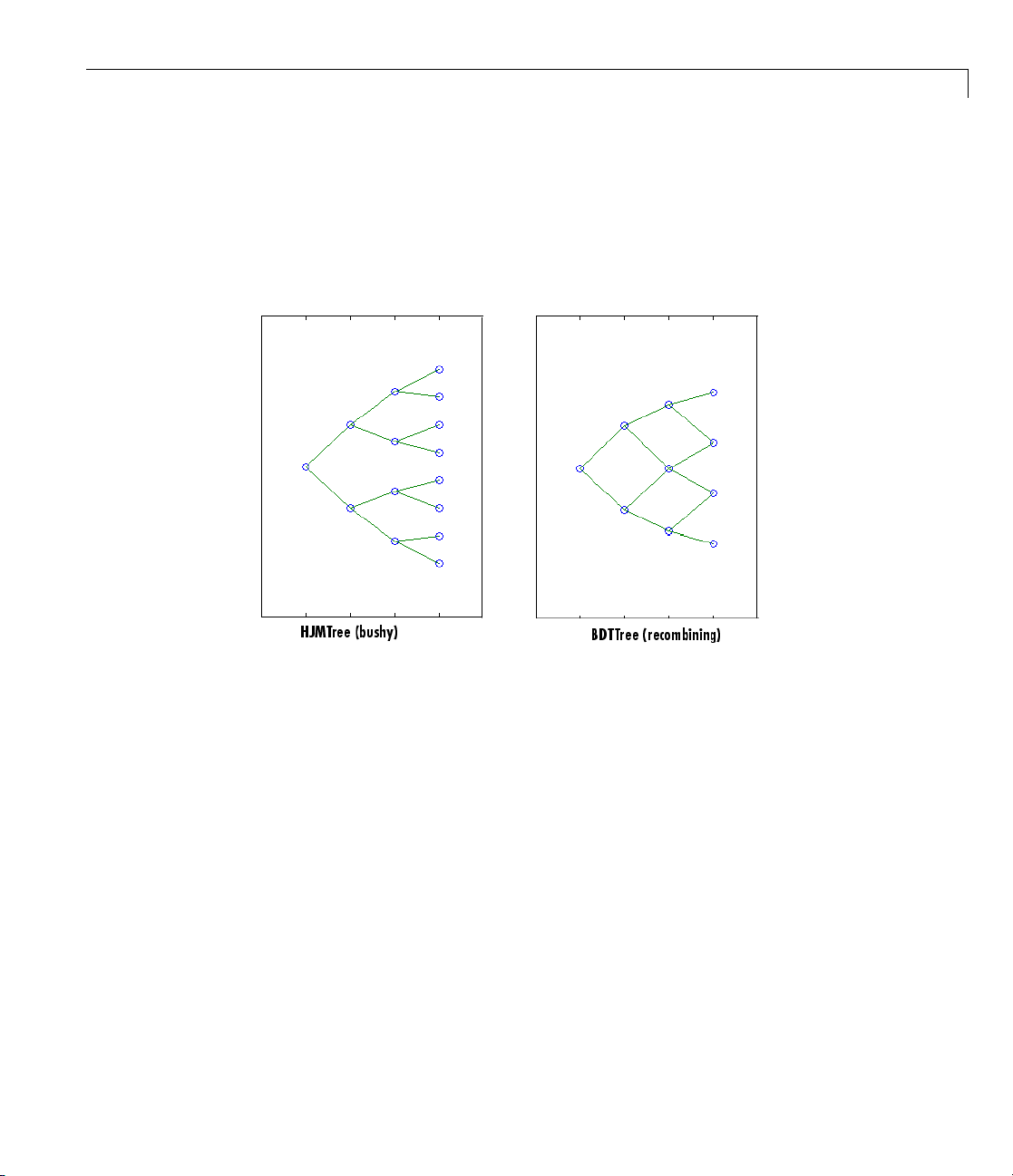
• HWTree and BKTree — Recombining trinomial trees

Overview of Interest-Rate Models

The toolbox also provides the

treeviewer function, w hich graphically displays

the shape and data of price, interest rate, and cash flow trees. Viewed with

treeviewer, the bushy shape of an HJM tree and the recombining shape

of a BDT tree are apparent.

With treeviewer, you can also see the recombining shape of HW and BK
trinomial trees.

2-13

2 Interest-Rate Derivatives

2-14

Understanding the Interest-Rate Term S tructure

Understanding the Interest-Rate Term Structure

In this section...

“Introduction” on page 2-15

“Interest Rates Versus Discount Factors” on page 2-15

“Interest-Rate Term Conversions” on page 2-20

“Functions That Model the Interest-Rate Term Structure” on page 2-24

Introduction

The interest-rate term structure represents the evolution of interest rates
through time. In MATLAB software, the interest-rate environment is
encapsulated in a structure called
structure holds all information required to completely identify the evolution
of interest rates. Several functions included in Financial Derivatives Toolbox
software are dedicated to the creating and managing of the
structure. Many others take this structure as an input argument representing
the evolution of interest rates.

RateSpec (rate specification). This

RateSpec

Before looking further at the
that provide key functio nality for working with interest rates:
opposite,
discount factors and interest rates. The third function,
the effect of term changes on the interest rates.

rate2disc,andratetimes. The first two functions map between

RateSpec structure, examine three functions

disc2rate,its

ratetimes,calculates

Interest Rates Versus Discount Factors

Discount factors are coefficients commonly used to find the current value
of future cash flows. As such, there is a direct mapping between the rate
applicable to a period of time, and the corresponding discount factor. The
function
interest rates. The function
rates applicable to a given term (period) into the corresponding discount
factors.

Calculating Discount Factors from Rates

As an example, consider these annualized zero-coupon bond rates.

disc2rate converts discount factors for a given term (period) into

rate2disc does the opposite; it converts interest

2-15

2 Interest-Rate Derivatives

From To Rate

15 Feb 2000

15 Aug 2000

15 Feb 2000 15 Feb 2 001

15 Feb 2000

15 Aug 2001

15 Feb 2000 15 Feb 2 002

15 Feb 2000

15 Aug 2002

0.05

0.056

0.06

0.065

0.075

To calculate the discount factors corresponding to these interest rates, call

rate2disc using the syntax

Disc = rate2disc(Compounding, Rates, EndDates, StartDates,
ValuationDate)

where:

•

Compounding represents the frequency at which the zero rates are

compounded when annualized. For this example, assume this value to be 2.

2-16

•

Rates is a vector of annualized percentage rates representing the interest

rate applicable to each time interval.

•

EndDates is a vector of date s representing the end of each interest-rate

term (period).

•

StartDates is a vector of dates representing the beginning of each

interest-rate term.

•

ValuationDate is the date of observation for which the discount factors

are calculated. In this particular example, use February 15, 2000 as the
beginning date for all interest-rate terms.

Next, set the variables in MATLAB.

StartDates = ['15-Feb-2000'];
EndDates = ['15-Aug-2000'; '15-Feb-2001'; '15-Aug-2001';...
'15-Feb-2002'; '15-Aug-2002'];
Compounding = 2;
ValuationDate = ['15-Feb-2000'];

Understanding the Interest-Rate Term S tructure

Rates = [0.05; 0.056; 0.06; 0.065; 0.075];

Finally, compute the discount factors.

Disc = rate2disc(Compounding, Rates, EndDates, StartDates,...
ValuationDate)

Disc =

0.9756

0.9463

0.9151

0.8799

0.8319

By adding a fourth column to the rates table (see “Calculating Discount
Factors from Rates” on page 2-15) to include the corresponding discounts, you
can see the evolution of the discount factors.

From To Rate Discount

15 Feb 2000

15 Aug 2000

15 Feb 2000 15 Feb 2001

15 Feb 2000

15 Aug 2001

15 Feb 2000 15 Feb 2002

15 Feb 2000

15 Aug 2002

0.05 0.9756

0.056 0.9463

0.06 0.9151

0.065 0.8799

0.075 0.8319

Optional Time Factor Outputs

The function rate2disc optionally returns two additional output argu ments:

EndTimes and StartTimes. These vectors of time factors represent the start

dates and end dates in discount periodic units. The scale of these units is
determined by the value of the input variable

To examine the time factor outputs, find the corresponding values in the
previous example.

[Disc, EndTimes, StartTimes] = rate2d isc(Compounding, Rates,...

Compounding.

2-17

2 Interest-Rate Derivatives

EndDates, StartDates, ValuationDate);

Arrange the two v ectors into a single array for easier visualization.

Times = [StartTimes, EndTimes]

Times =

01
02
03
04
05

Because the valuation date is equal to the start date for all periods, the

StartTimes vector is composed of 0s. Also, since the value of Compounding is

2, the rates are compounded semiannually, which sets the units o f periodic
discount to 6 months. The vector

EndDates is composed of dates separated

by intervals of 6 months from the valuation date. This explains why the

EndTimes vector is a progression of integers from 1 to 5.

2-18

Alternative Syntax (rate2disc)

The function rate2disc also accommodates an alternative syntax that uses
periodic discount units instead of dates. Since the relationship between
discount factors and interes t rates is based on time periods and not on
absolute dates, this form of
periods. In this mode, the valuation date corresponds to 0, and the vectors

StartTimes and EndTimes are used as input arguments instead of their date

equivalents,

Disc = rate2disc(Compounding, Rates, EndTimes, StartTimes)

StartDates and EndDates.Thissyntaxforrate2disc is:

Using as input the StartTimes and EndTimes vectors computed previously,
you should obtain the previous results for the discount factors.

Disc = rate2disc(Compounding, Rates, EndTimes, StartTimes)

Disc =

0.9756

rate2disc allows you to work directly with time

Understanding the Interest-Rate Term S tructure

0.9463

0.9151

0.8799

0.8319

Calculating Rates from Discounts

The function disc2rate is the complement to rate2disc.Itfindstherates
applicable to a set of compounding periods, given the discount factor in those
periods. The syntax for calling this func tion is:

Rates = disc2rate(Compounding, Disc, EndDates, StartDates,
ValuationDate)

Each argument to this function has the same meaning as in rate2disc.
Use the results found in the previous example to return the rate values you
started with.

Rates = disc2rate(Compounding, Disc, EndDates, StartDates,...
ValuationDate)

Rates =

0.0500

0.0560

0.0600

0.0650

0.0750

Alternative Syntax (disc2rate)

As in the case of r ate2disc, disc2rate optionally returns StartTimes and

EndTimes vectors representing the start and end times measured in discount

periodic units. Again, working with the same values as before, you should
obtain the same numbers.

[Rates, EndTimes, StartTimes] = disc2 rate(Compounding, Disc,...
EndDates, StartDates, ValuationDate);

Arrange the results in a matrix convenient to display.

2-19

2 Interest-Rate Derivatives

Result = [StartTimes, EndTimes, Rates]

Result =

0 1.0000 0.0500
0 2.0000 0.0560
0 3.0000 0.0600
0 4.0000 0.0650
0 5.0000 0.0750

As with rate2disc, the relationship between rates and discount factors is
determined by time periods and not by absolute dates. Consequently, the
alternate syntax for

disc2rate uses time vectors instead of dates, and it

assumes that the valuation date corresponds to time = 0. The time-based
calling syntax is:

Rates = disc2rate(Compounding, Disc, EndTimes, StartTimes);

Using this syntax, you again ob tain the original values for the interest rates.

2-20

Rates = disc2rate(Compounding, Disc, EndTimes, StartTimes)

Rates =

0.0500

0.0560

0.0600

0.0650

0.0750

Interest-Rate Term Conversions

Interest rate evolution is typically represented by a set of interest rates,
including the beginning and end of the periods the rates apply to. Fo r zero
rates, the start dates are typically at the valuation date, with the rates
extending from that valuation date until their respective maturity dates.

Spot Curve to Forward Curve Conversion

Frequently, given a set of rates including their start and end dates, you may
be interested in finding the rates a pp licable to different term s (periods). This

Understanding the Interest-Rate Term S tructure

problem is addressed by the function ratetimes. This function interpolates
the interest rates given a change in the original terms. The syntax for calling

ratetimes is

[Rates, EndTimes, StartTimes] = ratetimes(Compounding, RefRates,

RefEndDates, RefStartDates, EndDates, StartDates, ValuationDate);

where:

•

Compounding represents the frequency at which the zero rates are

compounded when annualized.

•

RefRates is a vector of initial interest rates representing the interest rates

applicable to the initial time intervals.

•

RefEndDates is a vector of dates representing the end of the interest rate

terms (period) applicable to

RefStartDates is a v ector of dates representing the beginning of the

•

interest rate terms applicable to

EndDates represent the maturity dates f or which the interest rates are

•

RefRates.

RefRates.

interpolated.

•

StartDates represent the starting dates for which the interest rates are

interpolated.

•

ValuationDate is the date of observation, from which the StartTimes and
EndTimes are calculated. This date represents time = 0.

The input arguments to this function can be separated into two groups:

• The initial or reference interest rates, including the terms for which they

are valid

• Terms for which the new interest rates are calculated

As an example, consider the rate table sp ecif ie d in “Calculating Discount
Factors from Rates” on page 2-15.

From To Rate

15 Feb 2000

15 Aug 2000

15 Feb 2000 15 Feb 2 001

0.05

0.056

2-21

2 Interest-Rate Derivatives

From To Rate

15 Feb 2000

15 Aug 2001

15 Feb 2000 15 Feb 2 002

15 Feb 2000

15 Aug 2002

0.06

0.065

0.075

Assuming that the valuation date is February 15, 2000, these rates represent
zero-coupon bond rates with maturities specified in the seco nd column. Use
the function

ratetimes to calculate the forward rates at the beginning of all

periods implied in the table. Assume a compounding value of 2.

% Reference Rates.
RefStartDates = ['15-Feb-2000'];
RefEndDates = ['15-Aug-2000'; '15-Feb-2001'; '15-Aug-2001';...
'15-Feb-2002'; '15-Aug-2002'];
Compounding = 2;
ValuationDate = ['15-Feb-2000'];
RefRates = [0.05; 0.056; 0 .06 ; 0.065; 0.075];

2-22

% New Terms.
StartDates = ['15-Feb-2000'; '15-Aug-2000'; '15-Feb-2001';...
'15-Aug-2001'; '15-Feb-2002'];
EndDates = ['15-Aug-2000 '; '15-Feb-2001 '; '15-Aug-2001 ';...
'15-Feb-2002'; '15-Aug-2002'];
% Find the new rates.
Rates = ratetimes(Compounding, RefRates, RefEndDates,...
RefStartDates, EndDates, StartDates, ValuationDate)

Rates =

0.0500

0.0620

0.0680

0.0801

0.1155

Placethesevaluesinatablelikethepreviousone. Observetheevolutionof
the forward rates based on the initial zero-coupon rates.

Understanding the Interest-Rate Term S tructure

From To Rate

15 Feb 2000

15 Aug 2000

15 Feb 2001

15 Aug 2001

15 Feb 2002

15 Aug 2000

15 Feb 2001

15 Aug 2001

15 Feb 2002

15 Aug 2002

0.0500

0.0620

0.0680

0.0801

0.1155

Alternative Syntax (ratetimes)

The ratetimes function can provide the additional output arguments

StartTimes and EndTimes, which represent the time factor equivalents to

the

StartDates and EndDates vectors. The ratetimes function uses time

factors for interpolating the rates. These time factors are calculated from
the start and end dates, and the valuation date, which are passed as input
arguments.
0 as the valuation date. This alternate syntax is:

ratetimes can also use time factors directly, assuming time =

[Rates, EndTimes, StartTimes] = rat etimes(Compounding, RefRates,
RefEndTimes, RefStartTimes, EndTimes, StartTimes);

Use this alternate version of ratetimes to find the forward rates again. In
this case, you must first find the time factors of the reference curve. Use

date2time for this.

RefEndTimes = date2time(ValuationDate, RefEndDates, Compounding)

RefEndTimes =

1
2
3
4
5

RefStartTimes = date2time(ValuationDate, RefStartDates,...
Compounding)

2-23

2 Interest-Rate Derivatives

RefStartTimes =

0

These are the expected values, given semiannual discounts (as denoted by a
value of 2 in the variable

Compounding),enddatesseparatedby6-month

periods, and the valuation date equal to the d ate marking beginning of the
first period (time factor = 0).

Now call

[Rates, EndTimes, StartTimes] = ratet imes(Compounding,...
RefRates, RefEndTimes, RefStartTimes, EndTimes, StartTimes);
Rates =

EndTimes

ratetimes with the alternate syntax.

0.0500

0.0620

0.0680

0.0801

0.1155

and StartTimes have, as expected, the same values they had as

input arguments.

Times = [StartTimes, EndTimes]

Times =

01
12
23
34
45

2-24

Functions That Model the Interest-Rate Term Structure

Financial Derivatives Toolbox software includes a set of functions to
encapsulate interest-rate term information into a single structure. These
functions present a convenient way to package all information related to

Understanding the Interest-Rate Term S tructure

interest-rate terms into a common format, and to resolve interdependencies
when one or more of the parameters is modified. For information, see:

• “Creating or Modifying (intenvset)” on page 2-25 for a discussion of how

to create or modify an interest-rate term structure (

intenvset function

RateSpec)usingthe

• “Obtaining Specific Properties (intenvget)” on page 2-27 for a discussion of

how to extract specific properties from a

RateSpec

Creating or Modifying (intenvset)

The main function to create o r modify an interest-rate term structure

RateSpec (rates specification) is in tenvset. If the first argument to this

function is a previously created
rate specification and returns a new one. Otherwise, it creates a

Use

intenvset to create or modify an interest-rate’s term structureRateSpec.

If the first argument to

intenvset is a previously created RateSpec,the

functionmodifiestheexistingratespecification and returns a ne w one;
otherwise,

intenvset creates a RateSpec.

RateSpec, the function modifies the e xisting

RateSpec.

When using

RateSpec to specify the rate term structure to price instruments

based on yields (zero coupon rates) or forward rates, specify zero rates or
forward rates as the input argument. However, the
limited or specific to this problem domain.
of rates-times relationships;
modifier, and

intenvget as an accessor. The interest rate m odels supported

intenvset acts as either a constructor or a

RateSpec is an encapsulation

RateSpec structure is not

by the Financial Derivatives Toolbox softw are work either with zero coupon
rates or forward rates .

The other

intenvset arguments are property-value pairs, indicating the new

value for these prope rti e s. The properties that can be specified or modified are:

•

Basis

• Compounding

• Disc

• EndDates

• EndMonthRule

2-25

2 Interest-Rate Derivatives

• Rates

• StartDates

• ValuationDate

To learn about the properties EndMonthRul e and Basis,type

help ftbEndMonthRule and help ftbBasis or see the Financial Toolbox

documentation.

Consider again the original table of interest rates (see “Calculating Discount
Factors from Rates” on page 2-15).

From To Rate

15 Feb 2000

15 Aug 2000

15 Feb 2000 15 Feb 2 001

15 Feb 2000

15 Aug 2001

15 Feb 2000 15 Feb 2 002

15 Feb 2000

15 Aug 2002

0.05

0.056

0.06

0.065

0.075

2-26

Use the information in this table to populate the

StartDates = ['15-Feb-2000'];
EndDates = ['15-Aug-2000 ';

'15-Feb-2001';
'15-Aug-2001';
'15-Feb-2002';

'15-Aug-2002'];
Compounding = 2;
ValuationDate = ['15-Feb-2000'];
Rates = [0.05; 0.056; 0.06; 0.065; 0.075];

rs = intenvset('Compounding',Compounding,'StartDates',...
StartDates, 'EndDates', EndDates, 'Rates', Rates,...
'ValuationDate', ValuationDate)

rs =

RateSpec structure.

Understanding the Interest-Rate Term S tructure

FinObj: 'RateSpec'

Compounding: 2

Disc: [5x1 double]

Rates: [5x1 double]

EndTimes: [5x1 double]

StartTimes: [5x1 double]

EndDates: [5x1 double]

StartDates: 730531

ValuationDate: 730531

Basis: 0

EndMonthRule: 1

Some of the properties filled in the structure were not passed explicitly in
the call to

RateSpec. The values of the automatically completed properties

depend on the properties that are explicitly passed. Consider for example
the

StartTimes and EndTimes vectors. Since the StartDates and EndDates

vectors are passed in, and the ValuationDate, intenvset has all the
information required to calculate

StartTimes and EndTimes.Hence,these

two properties are read-only.

Obtaining Specific Properties (intenvget)

The complementary function to intenvset is intenvget, which gets function
specific properties from the interest-rate term structure. Its syntax is:

ParameterValue = intenvget(RateSpec, 'ParameterName')

To obtain the vector EndTimes from the RateSpec s tructure, enter:

EndTimes = intenvget(rs, 'EndTimes')

EndTimes =

1
2
3
4
5

2-27

2 Interest-Rate Derivatives

To obtain Disc, the values for the discount factors that were calculated
automatically by

Disc = intenvget(rs, 'Disc')

Disc =

0.9756

0.9463

0.9151

0.8799

0.8319

intenvset,type:

These discount factors correspond to the periods starting from StartDates
and ending in EndDates.

Caution Although you can directly access these fields within the structure
instead of using

intenvget,itisadvisednottodoso. Theformatofthe

interest-rate term structure could change in future versions of the toolbox.
Should that happen, any code accessing the

RateSpec fields directly would

stop working.

2-28

Now use the RateSpec structure with its functions to examine how changes in
specific properties of the interest-rate term structure affect those depending
on it. As an exercise, change the value of

Compounding from 2 (semiannual)

to 1 (annual).

rs = intenvset(rs, 'Compounding', 1);

Since StartTimes and EndTimes are measured in units of periodic discount, a
change in

Compounding from 2 to 1 redefines the basic unit from semiannual

to annual. This means that a period of 6 months is represented with a value
of 0.5, and a period of 1 year is represented by 1. To obtain the vectors

StartTimes and EndTimes,enter:

StartTimes = intenvget(rs, 'StartTimes');
EndTimes = intenvget(rs, 'EndTimes');
Times = [StartTimes, EndTimes]

Understanding the Interest-Rate Term S tructure

Times =

0 0.5000
0 1.0000
0 1.5000
0 2.0000
0 2.5000

Since all the values in StartDates are t h e same as the valuation date, all

StartTimes values are 0. O n the other hand, the values in the EndDates

vector are d ate s separated by 6-month periods. Since the redefined value
of compounding is 1,

EndTimes becomes a sequence of numbers separated

by increments of 0.5.

2-29

2 Interest-Rate Derivatives

Computing Prices and Sensitivities Using the Interest-Rate
Term Structure

In this section...

“Introduction” on page 2-30

“Computing Instrument Prices” on page 2-31

“Computing Instrument Sensitivities” on page 2-33

Introducti

The instru
types of in
current ve
instrume

• Bonds

• Fixed-r

• Floatin

• Swaps

In addi
price a

Note t
above
beca
the e
pric
thes

Fin
the
com
su
Se

tion to these instruments, the toolbox also supports the calculation of

nd sensitivities of arbitrary sets of cas h flows.

hat options and interest-rate floors and caps are absent from the
list of supported instruments. These instruments are not supported

use their pricing and sensitivity function require a stochastic model for

volution of interest rates. The interest-rate term structure used for

ing is treated as deterministic, andassuchisnotadequateforpricing

e instruments.

ancial Derivatives Toolbox software also contains functions that use

Heath-Jarrow-Morton (HJM) and Black-Derman-Toy (BDT) models to

pute prices and sensitivities for financial instruments. These models
pport computations involving options and interest-rate floors and caps.
e “Computing Prices and Sensitivities Using Interest-Rate Tree Models”

on

ments can be presented to the functions as a portfolio of different

struments or as gro up s of instruments of the same ty pe . The

rsion of the toolbox can compute price and sensitivities for four

nt types using interest-rate curves:

ate notes

g-rate notes

2-30

Computing Prices and Sensitivities Using the Interest-Rate Term Structure

on page 2-62 for information on computing price and sensitivities of financial
instruments using the HJM and BDT models.

Computing Instrument Prices

The main f unction used for pricing portfolios of instruments is intenvprice.
This function works with the family of functions that calculate the prices of
individual types of instruments. When called,
portfolio contained in

InstSet by instrument type, and calls the appropriate

pricing functions. The map between instrument types and the pricing function

intenvprice calls is

intenvprice classifies the

bondbyzero:

fixedbyzero:

floatbyzero:

swapbyzero:

Price a bond by a set of zero curves

Price a fixed-rate note by a set of zero curves

Priceafloating-ratenotebyasetofzerocurves

Price a swap by a set of z ero curves

You can use each of these functions individually to price an instrument.
Consult the reference pages for specific information on using these functions.

intenvprice takes as input an interest-rate term structure created with
intenvset, and a portfolio of interest-rate contingent derivatives instruments

created with

instadd. To learn more about instadd and the interest-rate

term structure, see Chapter 1, “Getting Started”.

The syntax for using

Price = intenvprice(RateSpec, InstSet)

intenvprice to price an entire portfolio is

where:

•

RateSpec is the interest-rate term structure.

InstSet isthenameoftheportfolio.

•

2-31

2 Interest-Rate Derivatives

Example: Pricing a Portfolio of Instruments

Consider this example of using the intenvprice function to price a portfolio
of instruments supplied with Financial Derivatives Toolbox software.

The provided MAT-file
variable
structure

ZeroInstSet. The MAT-file also contains the interest-rate term

ZeroRateSpec. You can display the instruments with the function

deriv.mat stores a portfolio as an instrument set

instdisp.

load deriv.mat;

instdisp(ZeroInstSet)

Index Type CouponRate S ettle Maturity Period Basis...

1 Bond 0.04 01-Jan-2000 01-Jan-2003 1 NaN...

2 Bond 0.04 01-Jan-2000 01-Jan-2004 2 NaN...

Index Type CouponRate Settle Maturity FixedReset Basis...

3 Fixed 0.04 01-Jan-2000 01-Jan-2003 1 NaN...

Index Type Spread Settle Maturity FloatReset Basis...

4 Float 20 01-Jan-2000 01-Jan-2003 1 NaN...

Index Type LegRate Settle Maturity LegReset Basis...

5 Swap [0.06 20] 01-Jan-2000 01-Jan-2003 [1 1] NaN...

Use intenvprice to calculate the prices for the instruments contained in
the portfolio

format bank
Prices = intenvprice(ZeroRateSpec, ZeroInstSet)
Prices =

ZeroInstSet.

2-32

98.72

97.53

98.72

100.55

3.69

The output Prices is a vector containing the prices of all the instruments
in the portfolio in the order indicated by the

Index column displayed by

Computing Prices and Sensitivities Using the Interest-Rate Term Structure

instdisp. Consequently, the first two elements in Prices correspond to the

first two bonds; the third element corresponds to the fixed-rate note; the
fourth to the floating-rate note; and the fifth element corresponds to the price
of the swap.

Computing Instrument Sensitivities

In general, you can compute sensitivities either as dollar price changes or
as percentage price changes. The toolbox reports all sensitivities as dollar
sensitivities.

Using the interest-rate term structure, you can calculate two types of
derivative price sensitivities, delta and gamma. Delta represents the dollar
sensitivity of prices to shifts in the observed forward yield curve. Gamma
represents the dollar sensitivity of delta to shifts in the observed forward
yield curve.

The

intenvsens function computes instrument sensitivities and instrument

prices. If you need both the prices and sensitivity measures, use
A separate call to

intenvprice is not required.

intenvsens.

Here is the syntax

[Delta, Gamma, Price] = intenvsens( RateSpec, InstSet)

where, as before:

•

RateSpec is the interest-rate term structure.

InstSet isthenameoftheportfolio.

•

Example: Sensitivities and Prices

Here is an example that uses intenvsens to calculate both sensitivities and
prices.

format bank
load deriv.mat;
[Delta, Gamma, Price] = intenvsens(Ze roRateSpec, ZeroInstSet);

Display the results in a single matrix in bank format.

2-33

2 Interest-Rate Derivatives

All = [Delta Gamma Price]

All =

-272.64 1029.84 98.72

-347.44 1622.65 97.53

-272.64 1029.84 98.72

-1.04 3.31 100.55

-282.04 1059.62 3.69

To view the per-dollar sensitivity, divide the first two columns by the last one.

[Delta./Price, Gamma./Price, Price]

ans =

-2.76 10.43 98.72

-3.56 16.64 97.53

-2.76 10.43 98.72

-0.01 0.03 100.55

-76.39 286.98 3.69

2-34

Understanding Interest-Rate Tree Models

In this section...

“Introduction” on page 2-35

“Building a Tree of Forward Rates” on page 2-36

“Specifying the Volatility Model (VolSpec)” on page 2-38

“Specifying the Interest-Rate Term Structure (RateSpec)” on page 2-41

“Calibrating the Hull-White Model Using Market Data” on page 2-42

“Specifying the Time Structure (TimeSpec)” on page 2-47

“Examples of Tree Creation” on page 2-49

“Examining Trees” on page 2-50

Introduction

Financial Derivatives Toolbox software supports the Black-Derman-Toy
(BDT), Black-Karasinski (BK), Heath-Jarrow-Morton (HJM), an d Hull-White
(HW) interest-rate models. The Heath-Jarrow-Morton model is one of the
most widely used models for pricing interest-rate derivatives. The model
considers a given initial term structure of interest rates and a specification
of the volatility of forward rates to build a tree representing the evolution of
the interest rates, based on a statistical process. For further explanation,
see the book Modelling Fixed Income Securities and Interest Rate Options
by Robert A. Jarrow.

Understanding Interest-Rate Tree Models

The Black-De rman-Toy model is another analytical model commonly used for
pricing interest-rate derivatives. The model considers a given initial zero rate
term structure of interest rates and a specification of the yield volatilities of
long rates to build a tree representing the evolution of the interest rates. For
further explanation, see the paper “A One Factor Model of Interest Rates
and its Application to Treasury Bond Options” by Fischer Black, Emanuel
Derman, and William Toy.

The Hull-White model incorporates the initial term structure of interest rates
and the volatility term structure to build a trinomial recombining tree of short
rates. The resulting tree is used to value interest rate dependent securities.

2-35

2 Interest-Rate Derivatives

The implementation of the Hull-White model in Financial Derivatives Toolbox
software is limited to one factor.

The Black-Karasinski model is a s in gle factor, log-normal version of the
Hull-White model.

For further information on the Hull-White and Black-K a r asi n sk i models, see
the book Options, Futures, and Other Derivatives by John C. Hull.

Building a Tree of Forward Rates

The tree of forward rates is the fundamental unit representing the evolution
of interest rates in a given period of time. This section explains how to create
a f orw ard-rate tree using Financial Derivatives Toolbox software.

Note To avoid needle ss repetition, this document uses the HJM and BDT
models to illustrate the creation and use of interest-rate trees. T he HW and
BKmodelsaresimilartotheBDTmodel. Wherespecificdifferencesexist,
they are documented in “HW and BK Tree Structures” on page 2-57.

2-36

The MATLAB functions that create rate trees are hjmtree and bdttree.
The

hjmtree function creates the structure, HJMTree, containing time and

forward-rate information for a bushy tree. The
similar structure,

This structure is a self-contained unit that includes the tree of rates (found
in the
specifications used in bu i ld in g this tree.

These functions take three structures as input arguments:

• The volatility model

• The interest-rate term structure

• Thetreetimelayout

FwdTree field of the structure) and the volatility, rate, and time

(VolSpec)” on page 2-38.)

Interest-Rate Term Structure (RateSpec)” on page 2-41.)

(TimeSpec)” on page 2-47.)

BDTTree, for a recombining tree.

VolSpec. (See “Specifying the Volatility Model

RateSpec. (See “Specifying the

TimeSpec. (See “Specifying the Time Structure

bdttree function creates a

Understanding Interest-Rate Tree Models

An easy way to visualize any trees you create is with the treeviewer function,
which displays trees in a graphical manner. See “Graphical Representation of
Trees” on page 2-75 for information about

treeviewer.

Calling Sequence

The calling syntax for hjmtree is

HJMTree = hjmtree(VolSpec, RateSpec, TimeSpec)

Similarly, the calling syntax for bdttree is

BDTTree = bdttree(VolSpec, RateSpec, TimeSpec)

Each of these functions requires VolSpec, Rate Spec,andTimeSpec input
arguments:

•

VolSpec is a structure that specifies the forw ard-rate volatility process. You

create

VolSpec using either of the functions hjmvolspec or bdtvolspec.

hjmvolspec function supports the specification of up to three factors.

The
It handles these models for the volatility of the interest-rate term structure:

- Constant

- Stationary

- Exponential

- Vasicek

- Proportional

A one-factor model assumes that the interest term structure is affected by
a single source of uncertainty. Incorporating multiple factors allows you to
specify different types of shifts in the shape and location of the interest-rate
structure. See

bdtvolspec function supports only a single volatility factor. The

The
volatility remains constant between pairs of nodes on the tree. You supply
the input volatility values in a vector of decimal values. See
for details.

hjmvolspec for details.

bdtvolspec

2-37

2 Interest-Rate Derivatives

• RateSpec is the interest-rate specification of the initial rate curve. You

create this structure with the function
Model the Interest-Rate Term Structure” on page 2-24.)

•

TimeSpec isthetreetimelayoutspecification. Youcreatethisvariablewith

the functions
between level times and level dates for rate quoting. This structure
indirectly determines the number of levels in the tree.

hjmtimespec or bdttime spec . It represents the mapping

intenvset. (See “Functions That

Specifying th e Volatility Model (VolSpec)

Because HJM supports m ultifactor (up to 3) volatility models while BDT (also,
BK and HW) supports only a single volatility factor, the

bdtvolspec functions require different inputs and generate slightly different

outputs. For examples, see “Creating an HJM Volatility Model” on page 2-38.
For BDT examples see “Creating a BDT Volatility Model” on page 2-40.

Creating an HJM Volatility Model

The function hjmvolspec generates the structure VolSpec, which specifies

hjmvolspec and

2-38



tT,

the volat il ity process
this context capital T represents the starting time of the forward rate, and
t represents the observation time. The volatility process can be constructed
from a combination of factors specified sequentially in the call to function that
creates it. Each factor specification starts with a string specifying the name of
the factor, followed by the pertinent parameters.

HJM Volatility Specification Example. Consider an example that uses
a single factor, specifically, a constant-sigma factor. The constant factor
specification requires only one parameter, the value of
value corresponds to 0.10.

HJMVolSpec = hjmvolspec('Constant', 0.10)

HJMVolSpec =

FinObj: 'HJMVolSpec'

FactorModels: {'Constant'}

FactorArgs: {{1x1 cell}}
SigmaShift: 0
NumFactors: 1

()

used in the creation of the forward-rate trees. In



.Inthiscase,the

Understanding Interest-Rate Tree Models

NumBranch: 2

PBranch: [0.5000 0.5000]

Fact2Branch: [-1 1]

The NumFactors field of the VolSpec structure, VolSpec.NumFactors =

, reveals that the number of factors used to generate VolSpec was one.

1

The

FactorModels field indicates that it is a Constant factor, and the

NumBranches field indicates the number of branches. A s a consequence, each

node of the resulting tree has two branches, one going up, and the other
going down.

Consider now a two-factor volatility process made from a proportional factor
and an exponential factor.

% Exponential factor

Sigma_0 = 0.1;

Lambda = 1;

% Proportional factor

CurveProp = [0.11765; 0 .08825; 0.06865];

CurveTerm = [ 1 ; 2 ; 3 ];

% Build VolSpec

HJMVolSpec = hjmvolspec('Proportional', CurveProp, CurveTerm,...

1e6,'Exponential', Sigma_0, Lambda)

HJMVolSpec =

FinObj: 'HJMVolSpec'

FactorModels: {'Proportional' ' Exponential'}

FactorArgs: {{1x3 cell} {1x2 cell}}

SigmaShift: 0

NumFactors: 2

NumBranch: 3

PBranch: [0.2500 0.2500 0. 5000]

Fact2Branch: [2x3 double]

The output shows that the volatility specification was generated using two
factors. The tree has 3 branches per node. Each branch has probabilities of

0.25, 0.25, and 0.5, going from top to bottom.

2-39

2 Interest-Rate Derivatives

Creating a BDT Volatility Model

The function bdtvolspec generates the structure VolSpec, which specifies
the volatility process. The function requires three input arguments:

• The valuation date

ValuationDate

• The yield volatility end dates VolDates

• The yield volatility values VolCurve

An optional fourth argument InterpMethod, specifying the interpolation
method, can be included.

The syntax used for callin g

BDTVolSpec = bdtvolspec(ValuationDate, VolDates, VolCurve,...
InterpMethod)

bdtvolspec is:

where:

•

ValuationDate is the first observation date in the tree.

VolDates is a vector of dates representing yield volatility end dates.

•

VolCurve is a vector of yield volatility values.

•

InterpMethod is the method of interpolation to use. The default is linear.

•

BDT Volatility Specification Example. Consider the following example:

ValuationDate = datenum('01-01-2000');
EndDates = datenum(['01-01-2001'; '01-01-2002'; '01-01-2003';
'01-01-2004'; '01-01-2005']);
Volatility = [.2; .19; .18 ; .17; .16];

2-40

Use bdtvolsp ec to create a volatility specification. Because no interpolation
method is explicitly specified, the function uses the

BDTVolSpec = bdtvolspec(ValuationDate, EndDates, Volatility)

BDTVolSpec =

FinObj: 'BDTVolSpec'

ValuationDate: 730486

linear default.

Understanding Interest-Rate Tree Models

VolDates: [5x1 double]
VolCurve: [5x1 double]

VolInterpMethod: 'linear'

Specifying the Interest-Rate Term Structure (RateSpec)

The structure RateSpec is an interest term structure that defines the initial
forward-rate specification from which the tree rates are derived. “Functions
That M odel the Interest-Rate Term Structure” on page 2-24 explains how to
create these structures using the function
the starting and ending dates for each rate, and the compounding value.

Rate Specification Creation Example

Consider the following example:

Compounding = 1;
Rates = [0.02; 0.02; 0.02; 0.02];
StartDates = ['01-Jan-2000';

'01-Jan-2001';
'01-Jan-2002';
'01-Jan-2003'];

EndDates = ['01-Jan-2001 ';

'01-Jan-2002';
'01-Jan-2003';
'01-Jan-2004'];

ValuationDate = '01-Jan-2000';

intenvset, given the interest rates,

RateSpec = intenvset('Compounding',1,'Rates', Rates,...
'StartDates', StartDates, 'EndDates', EndDates,...
'ValuationDate', ValuationDate)

RateSpec =

FinObj: 'RateSpec'

Compounding: 1

Disc: [4x1 double]

Rates: [4x1 double]

EndTimes: [4x1 double]

StartTimes: [4x1 double]

EndDates: [4x1 double]

2-41

2 Interest-Rate Derivatives

StartDates: [4x1 double]

ValuationDate: 730486

Basis: 0

EndMonthRule: 1

Use the function datedisp to examine the dates defined in the variable

RateSpec. For example:

datedisp(RateSpec.ValuationDate)
01-Jan-2000

Calibrating the Hull-White Model Using Market Data

The pricing of interest rate derivative securities relies on models that describe
the underlying process. These interest rate models depend on one or more
parameters that you must determine by matching the m odel predictions to the
existing data available in the market. In the Hull-White model, there are two
parameters related to the short rate process: mean reversion and volatility.
Determining these parameters, such that the model is able to reproduce as
close a s possible the prices of caps or floors observed in the market, is called
calibration. T he calibration routines find the parameters that m inimize the
difference between the model price predictions and the market prices for
caps and floors.

2-42

In the case of the Hull-White model, the minimization is two dimensional
with respect to mean reversion (α)andvolatility(σ). That is, calibrating the
Hull-White model minimizes the dif ference between the model prices and
market prices for caps and floors:

(ModelPrice( , ) - MarketPrice)



(MarketPrice)

Hull-White Model Calibration Example

You can use hwcalbycap and hwcalbyfloor to determine the volatility
parameters, m ean reversion (α) and volatility (σ), such that the model fits the
prices of actively traded instruments for caps and floors as closely as possible.
Consider the following caplet market information:

MarketMat = {'21-Mar-2008';

'21-Jun-2008';

Understanding Interest-Rate Tree Models

'21-Sep-2008';

'21-Dec-2008';

'21-Mar-2009';

'21-Jun-2009';

'21-Sep-2009';

'21-Dec-2009';

'21-Mar-2010';

'21-Jun-2010';

'21-Sep-2010';

'21-Dec-2010';

'21-Mar-2011'};

MarketStrike = [0.0590; 0.0690; 0.0790];

MarketVol = [0.1533 0.1731 0.1727 0.1752 0.1809 0.1800 0.1805 0.1802 0.1735 0.1757 ...

0.1755 0.1755 0.1726;

0.1525 0.1725 0.1725 0.1750 0.1800 0.1800 0.1800 0.1800 0.1725 0.1750 ...

0.1750 0.1750 0.1725;

0.1526 0.1730 0.1726 0.1747 0.1808 0.1792 0.1797 0.1794 0.1733 0.1751 ...

0.1750 0.1745 0.1719];

1 Create RateSpec using the following data:

Rates= [0.0627;

0.0657;

0.0691;

0.0717;

0.0739;

0.0755;

0.0765;

0.0772;

0.0779;

0.0783;

0.0786;

0.0789;

0.0792;

0.0793];

ValuationDate = '21-Jan-2008';

EndDates = {'21-Mar-2008';'21-Jun-2008';'21-Sep-20 08';'21-Dec-2008';...

2-43

2 Interest-Rate Derivatives

'21-Mar-2009';'21-Jun-2009';'21-Sep-2009';'21-Dec-2009';....

'21-Mar-2010';'21-Jun-2010';'21-Sep-2010';'21-Dec-2010';....

'21-Mar-2011';'21-Jun-2011'};

Compounding = 4;

RateSpec = intenvset('ValuationDate', ValuationDate, ...

'StartDates', ValuationDate, 'EndDates', EndDates, ...

'Rates', Rates, 'Compounding', Compounding, 'Basis', 0);

2 Call the calibration routine to find the values for the volatility parameters

α and σ:

Settle = ' Jan-21-2008';

Maturity = 'Mar-21-2011';

Strike = 0.0690;

Reset = 4;

Principal = 1000;

Basis = 0;

o=optimset('TolFun',100*eps);

2-44

[Alpha, Sigma] = hwcalbycap(RateSpec, MarketStrike, MarketMat, MarketVol,...

Strike, Settle, Maturity, 'Reset', Reset, 'Principal', Principal, 'Basis',...

Basis, 'OptimOptions', o)

Warning: LSQNONLIN did not converge to an optimal solution. It exited with

exitflag = 2.

LSQNONLIN Diagnostic Message: '

Local minimum possible.

lsqnonlin stopped because the size of the current step is less than

the default value of the step size tolerance.

> In hwcalbycapfloor at 85

In hwcalbycap at 77

Alpha =

1.0000e-006

Understanding Interest-Rate Tree Models

Sigma =

0.0127

The warning above indicates that the conversion was not optimal. The
search algorithm used by the Optimization Toolbox™ function

lsqnonlin

could not find a solution that complies with all the constraints used by the
function. To d iscern whether the solution is acceptable, you must look at
the results of the optimization by specifying a third output (
for

hwcalbycap.

[Alpha, Sigma, OptimOut] = hwcalbycap(RateSpec, MarketStrike, MarketMat,...

MarketVol, Strike, Settle, Maturity, 'Reset', Reset, 'Principal', Principal,...

'Basis', Basis, 'OptimOptions', o);

OptimOut)

The OptimOut.residual field of the OptimOut structure is the optimization
residual. This value contains thedifferencebetweentheBlack
caplets and those calculated during the optimization. You can use the

OptimOut.residual value to calculate the percentual difference (error)

compared to Black Caplet prices and then decide whether the residual
is acceptable. There will almost always be some residual, so you must
decide if parametrizing the market with a single value of alpha and sigma
is acceptable.

3 You can price the caplets using the m arket data and Black’s formula to

obtain the reference caplet values:

MarketMatNum = datenum(MarketMat);

[Mats,Strikes] = meshgrid(MarketMatNum, MarketStrike);

FlatVol = interp2(MarketMatNum, MarketStrike, MarketVol, datenum(Maturity),. ..

Strike, 'spline');

[CapPrice, Caplets] = c apbyblk(RateSpec, Strike, Settle, M aturity, FlatVol,...

'Reset', Reset, 'Basis', Basis, 'Principal', Principal);

Caplets = Caplets(2:end)';

4 You can compare the optimized values and the Black values and display

graphically:

OptimCaplets = Caplets+OptimOut.residual;

disp([Caplets OptimCaplets])

plot(MarketMatNum(2:end), Caplets, 'or', MarketMatNum(2:end), OptimCaplets, '*b');

2-45

2 Interest-Rate Derivatives

datetick('x', 2)

xlabel('Caplet Maturity');

ylabel('Caplet Price');

title('Black and Calibrated Caplets');

h = legend('Black Caplets', 'Calibrated Caplets');

set(h, 'color', [0.9 0.9 0.9]);

set(h, 'Location', 'SouthEast');

set(gcf, 'NumberTitle', 'off')

grid on

0.3216 0.3643

1.6363 1.6612

2.4872 2.4983

3.1912 3.1883

3.4121 3.4051

3.2698 3.2653

3.2400 3.2379

3.4819 3.4699

3.2437 3.2426

3.1968 3.1977

3.3011 3.2980

3.3771 3.3684

2-46

5 To visualize this, consider the following comparison:

Understanding Interest-Rate Tree Models

Specifying the Time Structure (TimeSpec)

The structure TimeSpec specifies the time structure for an interest-rate tree.
This structure defines the mapping between the observation times at each
level of the tree and the corresponding dates.

TimeSpec is built using either the hjmtimes pec or bdttimespec function.

These functions require three input arguments:

• The valuation date

• The maturity date Maturity

• The compounding rate Compounding

For example, the syntax used for calling hjmtimespec is

TimeSpec = hjmtimespec(ValuationDate, Maturity, Compounding)

where:

ValuationDate

2-47

2 Interest-Rate Derivatives

• ValuationDate is the first observation date in the tree.

Maturity is a vector of dates representing the cash flow dates of the tree.

•

Any instrument cash flo ws with these maturities fall on tree nodes.

•

Compounding is the frequency at which the rates are compounded when

annualized.

Creating a Time Specification

Calling the time specification creation functions with the same data used to
create the interest-rate term structure,
specifies the time layout for the tree.

HJM Time Specificatio n Example. Consider the following example:

Maturity = EndDates;
HJMTimeSpec = hjmtimespec(ValuationDate, Maturity, Compounding)

HJMTimeSpec =

RateSpec builds the structure that

2-48

FinObj: 'HJMTimeSpec'

ValuationDate: 730486

Maturity: [4x1 double]

Compounding: 1

Basis: 0

EndMonthRule: 1

Note that maturities specified when building TimeSpec need not coincide
with the
the time-date mapping of the tree, the rates in
obtain the initial rates with m aturities equal to those in

EndDates oftherateintervalsinRateSpec.SinceTimeSpec defines

RateSpec are interpolated to

TimeSpec.

Creating a BDT Time Specification. Consider the following example:

Maturity = EndDates;
BDTTimeSpec = bdttimespec(ValuationDate, Maturity, Compounding)

BDTTimeSpec =

FinObj: 'BDTTimeSpec'

ValuationDate: 730486

Understanding Interest-Rate Tree Models

Maturity: [4x1 double]

Compounding: 1

Basis: 0

EndMonthRule: 1

Examples of Tree Creation

Use the VolSpec, RateSpec,andTimeSpec you have previously created as
inputs to the functions used to create HJM and BDT trees.

Creating an HJM Tree

% Reset the volatility factor to the Constant case

HJMVolSpec = hjmvolspec('Constant', 0.10);

HJMTree = hjmtree(HJMVolSpec, RateSpec, HJMTimeSpec)

HJMTree =

FinObj: 'HJMFwdTree'

VolSpec: [1x1 struct]

TimeSpec: [1x1 struct]

RateSpec: [1x1 struct]

tObs: [0 1 2 3]

TFwd: {[4x1 double] [3x1 double] [2x1 double] [3]}

CFlowT: {[4x1 double] [3x1 double] [2x1 double] [4]}

FwdTree:{[4x1 double][3x1x2 double][2x2x2 double][1x4x2 double]}

Creating a BDT Tree

Now use the previously computed values for VolSpec, RateSpec,and

TimeSpec as input to the function bdttree to create a BDT tree.

BDTTree = bdttree(BDTVolSpec, RateSpec, BDTTimeSpec)

BDTTree =

FinObj: 'BDTFwdTree'

VolSpec: [1x1 struct]

TimeSpec: [1x1 struct]

2-49

2 Interest-Rate Derivatives

RateSpec: [1x1 struct]

tObs: [0 1.00 2.00 3.00]

TFwd: {[4x1 double] [3x1 double] [2x1 double] [3.00]}

CFlowT: {[4x1 double] [3x1 double] [2x1 double] [4.00]}

FwdTree: {[1.02] [1.02 1.02] [1.01 1.02 1.03] [1.01 1.02 1.02 1.03]}

Examining Trees

When working with the m odels, Financial Derivatives Toolbox software uses
trees to represent forward rates, prices, and so on. At the highest level, these
trees have structures wrapped around them. The structures encapsulate
information required to interpret completely the information contained in a
tree.

Consider this example, which uses the interest rate and portfolio data in the
MAT-file

Load the data into the MATLAB workspace.

load deriv.mat

deriv.mat included in the toolbox.

2-50

Display the list of the variables loaded from the MAT-file.

whos

Name Size Bytes Class Attributes

BDTInstSet 1x1 15956 struct
BDTTree 1x1 5138 struct
BKInstSet 1x1 15946 struct
BKTree 1x1 5904 struct
CRRInstSet 1x1 12434 struct
CRRTree 1x1 5058 struct
EQPInstSet 1x1 12434 struct
EQPTree 1x1 5058 struct
HJMInstSet 1x1 15948 struct
HJMTree 1x1 5838 struct
HWInstSet 1x1 15946 struct
HWTree 1x1 5904 struct
ITTInstSet 1x1 12438 struct
ITTTree 1x1 8862 struct

Understanding Interest-Rate Tree Models

ZeroInstSet 1x1 10 282 struct
ZeroRateSpec 1x1 1580 struct

HJM Tree Structure

You can now examine in some detail the contents of the HJMTree structure
contained in this file.

HJMTree

HJMTree =

FinObj: 'HJMFwdTree'

VolSpec: [1x1 struct]

TimeSpec: [1x1 struct]

RateSpec: [1x1 struct]

tObs: [0 1 2 3]

TFwd: {[4x1 double] [3x1 double] [2x1 double] [3]}

CFlowT: {[4x1 double] [3x1 double] [2x1 double] [4]}

FwdTree:{[4x1 double][3x1x2 double][2x2x2 double][1x4x2 double]}

FwdTree contains the actual forward-rate tree. MATLAB software represents

it as a cell array with each cell array element containing a tree level.

The other fields contain other information relevant to interpreting the values
in

FwdTree. The most important are VolSpec, TimeSpec,andRateSpec,

which contain the volatility, time structure, and rate structure information
respectively.

First Node. Observe the forward rates in
the valuation date,

HJMTree.FwdTree{1}

ans =

1.0356

1.0468

1.0523

1.0563

tObs = 0.

FwdTree. The first node represents

2-51

2 Interest-Rate Derivatives

Note Financial Derivatives Toolbox software uses inverse discount notation

for forward rates in the tree. An inverse discount repre sents a factor by which
thecurrentvalueofanassetismultiplied to find its future value. In general,
these forward factors are reciprocals of the discount factors.

Look closely at the RateSpec structure used in generating this tree to see
where these values originate. Arrange the values in a single array.

[HJMTree.RateSpec.StartTimes HJMTree.RateSpec.EndTimes...
HJMTree.RateSpec.Rates]

ans =

0 1.0000 0.0356

1.0000 2.0000 0.0468

2.0000 3.0000 0.0523

3.0000 4.0000 0.0563

2-52

If you find the corresponding inverse discounts of the interest rates in the
third column, you have the values at the first node of the tree. You can turn
interest rates into inverse discounts using the function

Disc = rate2disc(HJMTree.TimeSpec.Compounding,...
HJMTree.RateSpec.Rates, HJMTree.RateSpec.EndTimes,...
HJMTree.RateSpec.StartTimes);
FRates = 1./Disc

FRates =

1.0356

1.0468

1.0523

1.0563

rate2disc.

Second Node. The second node represents the first-rate obs ervation time,

tObs = 1. This node displays two states: one representing the branch going

up and the other representing the branch going down.

Note that

HJMTree.VolSpec.NumBranch = 2.

Understanding Interest-Rate Tree Models

HJMTree.VolSpec

ans =

FinObj: 'HJMVolSpec'

FactorModels: {'Constant'}

FactorArgs: {{1x1 cell}}
SigmaShift: 0
NumFactors: 1

NumBranch: 2

PBranch: [0.5000 0.5000]

Fact2Branch: [-1 1]

Examine the rates of the node corresponding to the up branch.

HJMTree.FwdTree{2}(:,:,1)

ans =

1.0364

1.0420

1.0461

Now examine the corresponding down branch.

HJMTree.FwdTree{2}(:,:,2)

ans =

1.0574

1.0631

1.0672

Third Node. The third node represents the second observation time, tObs

. This node contains a total of four states, two representing the branches

=2

going up and the other two representing the branches going down. Examine
the rates of the node corresponding to the up states.

HJMTree.FwdTree{3}(:,:,1)

ans =

2-53

2 Interest-Rate Derivatives

1.0317 1.0526

1.0358 1.0568

Next examine the corresponding down states.

HJMTree.FwdTree{3}(:,:,2)

ans =

1.0526 1.0738

1.0568 1.0781

Isolating a Specific Node. Starting at the third level, indexing within the
tree cell array becomes complex, and isolating a specific node can be difficult.
The function

bushpath isolates a specific node by specifying the path to

the node as a vector of branches takentoreachthatnode. Asanexample,
consider the node reached by starting from the roo t node, taking the branch
up, then the branch down, and then another branch down. Given that the tree
has only two branches per node, branches going up correspond to a 1, and
branches going down co rrespond to a 2. The path up-down-down becomes the
vector

[1 2 2].

2-54

FRates = bushpath(HJMTree.FwdTree, [1 2 2])

FRates =

1.0356

1.0364

1.0526

1.0674

bushpath

returns the spot rates for all the nodes touched by the path specified
in the input argument, the first one corresponding to the root node, and the
last one corresponding to the target node.

Isolating the same node using direct indexing obtains

HJMTree.FwdTree{4}(:, 3, 2)

Understanding Interest-Rate Tree Models

ans =

1.0674

As expected, this single value corres ponds to the las t element of the rates
returned by

bushpath.

You can use these techniques with any type of tree generated with Financial
Derivatives Toolbox software, such as forward-rate trees or price trees.

BDT Tree Structure

You can now examine in some detail the contents of the BDTTree structure.

BDTTree

BDTTree =

FinObj: 'BDTFwdTree'

VolSpec: [1x1 struct]
TimeSpec: [1x1 struct]
RateSpec: [1x1 struct]

tObs: [0 1 2 3]
TFwd: {[4x1 double] [3x1 double] [2x1 double] [ 3]}

CFlowT: {[4x1 double] [3x1 double] [2x1 double] [ 4]}

FwdTree: {1x4 cell}

FwdTree

contains the actual rate tree. MATLAB software represents it as a

cell array with each cell array element containing a tree level.

The other fields contain other information relevant to interpreting the values
in

FwdTree. The most important are VolSpec, TimeSpec,andRateSpec,

which contain the volatility, time structure, and rate structure information
respectively.

Look at the

RateSpec structure u sed in generating this tree to see where

these values originate. Arrange the values in a single array.

[BDTTree.RateSpec.StartTimes BDTTree.RateSpec.EndTimes...
BDTTree.RateSpec.Rates]

2-55

2 Interest-Rate Derivatives

ans =

0 1.0000 0.1000
0 2.0000 0.1100
0 3.0000 0.1200
0 4.0000 0.1250

Look at the rates in FwdTree. The first node represents the valuation date,

tObs = 0. The second node represents tObs = 1. Examine the rates at the

second, third, and fourth nodes.

BDTTree.FwdTree{2}

ans =

1.0979 1.1432

The second node represents the first observation time, tObs = 1.Thisnode
contains a total of two states, one representing the branch going up (
and the other representing the branch going down (

1.1432).

1.0979)

2-56

Note The convention in this document is to display prices going up on the
upper branch. Consequently, when displaying rates, rates are falling on the
upper branch and increasing on the lower branch.

BDTTree.FwdTree{3}

ans =

1.0976 1.1377 1.1942

The third node represents the second observation time, tObs = 2.This
node contains a total of three s tates, one representing the branch going up
(

1.0976), one representin g the branch in the middle (1.1377) a nd the other

representing the branch going down (

BDTTree.FwdTree{4}

1.1942).

Understanding Interest-Rate Tree Models

ans =

1.0872 1.1183 1.1606 1.2179

The fourth node represents the third observation time, tObs = 3.Thisnode
contains a total of four states, one representing the branch going up (
tworepresentingthebranchesinthemiddle(
other representing the branch going down (

1.1183 and 1.1606), and the

1.2179).

1.0872),

Isolating a Specific Node. The function

treepath isolates a specific node

by specifying the path to the node as a vector of branches taken to reach that
node. As an example, consider the node reached by starting from the root
node, taking the branch up, then the branch down, and finally another branch
down. Given that the tree h as only two branches per node, branches going
up correspond to a 1, and branches going down correspond to a 2. The path
up-down-down becomes the vector

FRates = treepath(BDTTree.FwdTree, [1 2 2])

FRates =

1.1000

1.0979

1.1377

1.1606

treepath

returns the short rates for all the nodes touched by the path

[1 2 2].

specified in the input argument, the first one corresponding to the root node,
and the last one corresponding to the targ et node.

HW and BK Tree Structures

The HW and BK tree s tructures are similar to the BDT tree structure. You can
see this if you examine the sample HW tree contained in the file

deriv.mat.

load deriv.mat:

HWTree

FinObj: 'HWFwdTree'
VolSpec: [1x1 struct]

2-57

2 Interest-Rate Derivatives

TimeSpec: [1x1 struct]
RateSpec: [1x1 struct]
tObs: [0 1 2 3]
dObs: [731947 732313 73267 8 733043]
CFlowT: {[4x1 double] [3x1 double] [2x1 double] [4]}
Probs: {[3x1 double] [3x3 double] [3x5 double]}
Connect: {[2] [2 3 4] [2 2 3 4 4]}
FwdTree: {1x4 cell}

All fields of this structure are similar to their BDT counterparts. There are
two additional fields not present in BDT:

Probs an d Connect.TheProbs field

represents the occurrence probabilities at each branch of each node in the
tree. The

Connect field describes the connectivity of the nodes of a given tree

level to nodes to the next tree level.

Probs Field. While BDT and one-factor HJM models have equal probabilities
for each branch at a node, HW and BK do not. For HW and BK trees, the

Probs field indicates the l ikelihood that a particular branch will be ta ken in

moving from one node to another node on the next level.

2-58

The

Probs field consists of a cell array with 1 cell per tree level. Each cell

is a

3-by-NUMNODES array with the top row representing the probability of

an up movement, the middle row representing the probability of a middle
movement, and the last row the probability of a down movement.

As an illustration, consider the first two elements of the

Probs field of the

structure, corresponding to the first (root) and second levels o f the tree.

HWTree.Probs{1}

0.16666666666667

0.66666666666667

0.16666666666667

HWTree.Probs{2}

0.12361333418768 0.16666666666667 0.21877591615172

0.65761074966060 0.66666666666667 0.65761074966060

0.21877591615172 0.16666666666667 0.12361333418768

Understanding Interest-Rate Tree Models

Reading from top to bottom, the values in HWTree. Probs{1} correspond to the
up, middle, and down probabilities at the root node.

HWTree.Probs{2} is a 3-by-3 matrix of values. The first column represents the

top node, the second column represents the middle node, and the last column
represents the bottom node. As with the root node, the first, second, and third
rows hold the values for up, middle, and down branching off each node.

As expected, the sum of all the probabilities at any node equals 1.

sum(HWTree.Probs{2})

1.0000 1.0000 1.0000

Connect Field. The other field that distinguishes HW and BK tree structures
from the BDT tree structure is

Connect. This field describes how each node in

a given level connects to the nodes of the next level. The need for this field
arises from the possibility of nonstandard branching in a tree.

The

Connect field of the HW tree structure consists of a cell array with 1

cell per tree level.

HWTree.Connect

ans =

[2] [1x3 double] [1x5 double]

Each cell contains a 1-by-NUMNODES vector. Each value in the vector relates to
a node in the corresponding tree level and represents the index of the node in
thenexttreelevelthatthemiddlebranchofthenodeconnectsto.

If yo u subtract 1 from the values contained in

Connect, you reveal the index

of the nodes in the next leve l that the up branch connects to. If you add 1 to
the values, you reveal the index of the corresponding down branch.

As an illustration , consider

HWTree.Connect{1}

ans =

HWTree.Connect{1}:

2-59

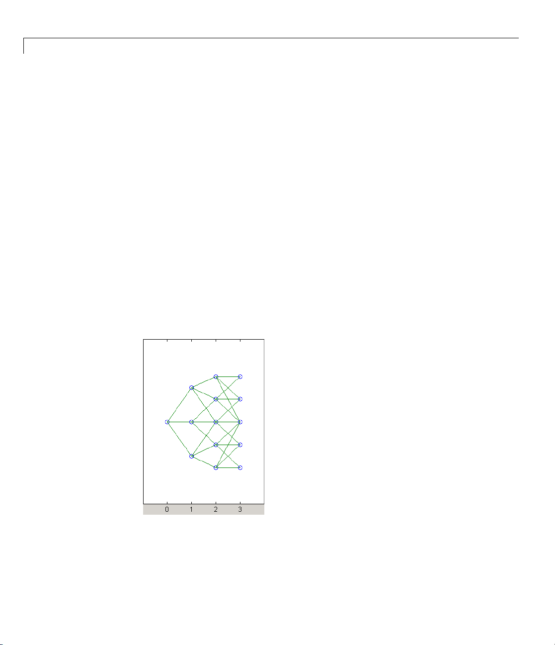
2 Interest-Rate Derivatives

2

This indicates that the middle branch of the root node connects to the second
(from the top) node of the next level, as expected. If you subtract 1 from
this value, you obtain 1, which tells you that the up branch goes to the top
node. If you add 1, you obtain 3, which points to the last node of the second
level of the tree.

Now consider lev el 3 in this example:

HWTree.Connect{3}

22344

On this level, there is nonstandard branching. Thi s can be easily recognized
because the middle branch of two nodes is connected to the same node on
the next level.

2-60

To visualize this, consider the following illustration of the tree.

Here it becomes apparent that there is nonstandard branching at the third
level of the tree, on the top and bottom nodes. The first and second nodes

Understanding Interest-Rate Tree Models

connect to the same trio of nodes on the next level. Similar branching occurs
at the bottom and next-to-bottom nodes of the tree.

2-61

2 Interest-Rate Derivatives

Computing Prices and Sensitivities Using Interest-Rate
Tree Models

In this section...

“Introduction” on page 2-62

“Computing Instrument Prices” on page 2-62

“Computing Instrument Sensitivities” on page 2-71

Introducti

For purpos
The HW and B
are not exp
operate s

Computi

The port
of any se
functio

• Bonds

• Bond op

• Arbit

• Fixed

• Floa

• Caps

• Flo

• Swa

es of illustration, this section relies on the HJM and BDT models.

licitly shown here. Functions that use the HW and BK models

imilarly to the BDT model.

ng Instrument Prices

folio pricing functions

t of supported instruments, based on an interest-rate tree. The

ns are capable of pricing these instrument types:

tions

rary cash flows

-rate notes

ting-rate notes

ors

ps

on

K functions that perform price and sensitivity computations

hjmprice and bdtprice calculate the price

2-62

• Swa

Fo

ptions

r example, the syntax for calling

hjmprice is:

Computing Prices and Sensitivities Using Interest-Rate Tree Models

[Price, PriceTree] = hj mprice(HJMTree, InstSet, Options)

Similarly, the calling syntax for bdtpr ice is:

[Price, PriceTree] = bd tprice(BDTTree, InstSet, Options)

Each function requires two input arguments: the interest-rate tree and the
set of instruments,

InstSet. An optional argument Options further controls

the p ricing and the output displayed. (See Appendix A, “Derivatives Pricing
Options” for information about the

HJMTree is the Heath-Jarrow-Morton tree sampling of a forward-rate process,

created using

hjmtree. BDTTree is the Black-Derman-Toy tree sampling of an

interest-rate process, created using

Options argument.)

bdttree. See “Building a Tree of Forward

Rates” on page 2-36 to learn how to create these structures.

InstSet is the set of instruments to be priced. This structure represents the

set of instruments to be priced independently using the model. Chapter 1,
“Getting Started”, explains how to create this variable.

Options is an options structure created with the function derivset.This

structure defines how the tree is used to find the price of instruments in the
portfolio, and how m uch additional information is displayed in the command
window when calling the pricing function. If this input argument is not
specified in the call to the pricing function, a default Options structure is
used. The pricing options structure is described in “Pricing Options Structure”
on page A-2.

The portfolio pricing functions classify the instruments and call the
appropriate instrument-specific pricing function for each of the instrument
types. The HJM instrument-specific pricing functions are

cfbyhjm, fixedbyhjm, floatbyhjm, optbndbyhjm, swapbyhjm,and
swaptionbyhjm. A similarly n amed set of functions exists for BDT models.

bondbyhjm,

For a list of these, see “Black-Derman-Toy Trees” on page 5-4.

You can also use these functions directly to calculate the price of sets of
instruments of the same type. See Chapter 6, “Functions — Alphabetical List”
for these individual functions for further information.

2-63

2 Interest-Rate Derivatives

HJM Pricing Example

Consider the following example, which uses the portfolio and interest-rate
data in the MAT-file
the MATLAB workspace.

load deriv.mat

Use the MATLAB whos command to display a list of the variables loaded
from the MAT-file.

whos

Name Size Bytes Class Attributes

BDTInstSet 1x1 15956 struct
BDTTree 1x1 5138 struct
BKInstSet 1x1 15946 struct
BKTree 1x1 5904 struct
CRRInstSet 1x1 12434 struct
CRRTree 1x1 5058 struct
EQPInstSet 1x1 12434 struct
EQPTree 1x1 5058 struct
HJMInstSet 1x1 15948 struct
HJMTree 1x1 5838 struct
HWInstSet 1x1 15946 struct
HWTree 1x1 5904 struct
ITTInstSet 1x1 12438 struct
ITTTree 1x1 8862 struct
ZeroInstSet 1x1 10 282 struct
ZeroRateSpec 1x1 1580 struct

deriv.mat included in the toolbox. Load the data into

2-64

HJMTree

function

and HJMInstSet are the input arguments required to call the

hjmprice.

Use the function
variable

HJMInstSet.

instdisp to examine the set of instruments contained in the

Computing Prices and Sensitivities Using Interest-Rate Tree Models

instdisp(HJMInstSet)

Index Type CouponRate Settle Maturity Period Basis ... Name Quantity

1 Bond 0.04 01-Jan-2000 01-Jan-2003 1 NaN ... 4% bond 100

2 Bond 0.04 01-Jan-2000 01-Jan-2004 2 NaN ... 4% bond 50

Index Type UnderInd OptSpec Strike ExerciseDates AmericanOpt Name Quantity

3 OptBond 2 call 101 01-Jan-2003 NaN Option 101 -50

Index Type CouponRate Settle Maturity FixedReset Basis Principal Name Quantity

4 Fixed 0.04 01-Jan-2000 01-Jan-2003 1 NaN NaN 4% Fixed 80

Index Type Spread Settle Maturity FloatReset Basis Principal Name Quantity

5 Float 20 01-Jan-2000 01-Jan-2003 1 NaN NaN 20BP Float 8

Index Type Strike Settle Maturity CapReset Basis Principal Name Quantity

6 Cap 0.03 01-Jan-2000 01-Jan-2004 1 NaN NaN 3% Cap 30

Index Type Strike Settle Maturity FloorReset Basis Principal Name Quantity

7 Floor 0.03 01-Jan-2000 01-Jan-2004 1 NaN NaN 3% Floor 40

Index Type LegRate Settle Maturity LegReset Basis Principal LegType Name Quantity

8 Swap [0.06 20] 01-Jan-2000 01-Jan-2003 [1 1] NaN NaN [NaN] 6%/20BP Swap 10

Note that there ar e eight instruments in this portfolio set: two bonds, one
bond option, one fixed-rate note, one floating-rate note, one cap, one floor, and
one swap. Each instrument has a corresponding index that identifies the
instrument prices in the price vector returned by

Now use

hjmprice to calculate the price of each instrument in the instrument

hjmprice.

set.

Price = hjmprice(HJMTree, HJMInstSet)

Warning: Not all cash flows are aligned with the tree. Re sult will

be approximated.

Price =

2-65

2 Interest-Rate Derivatives

98.7159

97.5280

0.0486

98.7159

100.5529

6.2831

0.0486

3.6923

Note The warning shown above appears because some of the cash flows for
the second bond do not fall exactly on a tree node.

BDT Pricing Example

Load the MAT-file deriv.mat into the MATLAB workspace.

load deriv.mat

2-66

Use the MATLAB whos command to display a list of the variables loaded
from the MAT-file.

whos

Name Size Bytes Class Attributes

BDTInstSet 1x1 15956 struct
BDTTree 1x1 5138 struct
BKInstSet 1x1 15946 struct
BKTree 1x1 5904 struct
CRRInstSet 1x1 12434 struct
CRRTree 1x1 5058 struct
EQPInstSet 1x1 12434 struct
EQPTree 1x1 5058 struct
HJMInstSet 1x1 15948 struct
HJMTree 1x1 5838 struct
HWInstSet 1x1 15946 struct
HWTree 1x1 5904 struct
ITTInstSet 1x1 12438 struct

Computing Prices and Sensitivities Using Interest-Rate Tree Models

ITTTree 1x1 8862 struct
ZeroInstSet 1x1 10 282 struct
ZeroRateSpec 1x1 1580 struct

BDTTree

function

Use the function
variable

instdisp(BDTInstSet)

Index Type CouponRate Settle Maturity Period Basis ........ Name Quantity

1 Bond 0.1 01-Jan-2000 01-Jan-2003 1 NaN......... 10% bond 100

2 Bond 0.1 01-Jan-2000 01-Jan-2004 2 NaN......... 10% bond 50

Index Type UnderInd OptSpec Strike ExerciseDates AmericanOpt Name Quantity

3 OptBond 1 call 9501 Jan-2002 NaN Option 95 -50

Index Type CouponRate Settle Maturity FixedReset Basis Principal Name Quantity

4 Fixed 0.10 01-Jan-2000 01-Jan-2003 1 NaN NaN 10% Fixed 80

Index Type Spread Settle Maturity FloatReset Basis Principal Name Quantity

5 Float 20 01-Jan-2000 01-Jan-2003 1 NaN NaN 20BP Float 8

and BDTInstSet are the input arguments required to call the

bdtprice.

instdisp to examine the set of instruments contained in the

BDTInstSet.

Index Type Strike Settle Maturity CapReset Basis Principal Name Quantity

6 Cap 0.15 01-Jan-2000 01-Jan-2004 1 NaN NaN 15% Cap 30

Index Type Strike Settle Maturity FloorReset Basis Principal Name Quantity

7 Floor 0.09 01-Jan-2000 01-Jan-2004 1 NaN NaN 9% Floor 40

Index Type LegRate Settle Maturity LegReset Basis Principal LegType Name Quantity

8 Swap [0.15 10] 01-Jan-2000 01-Jan-2003 [1 1] NaN NaN [NaN] 15%/10BP Swap 10

2-67

2 Interest-Rate Derivatives

Note that there ar e eight instruments in this portfolio set: two bonds, one
bond option, one fixed-rate note, one floating-rate note, one cap, one floor, and
one swap. Each instrument has a corresponding index that identifies the
instrument prices in the price vector returned by

bdtprice.

Now use

bdtprice to calculate the price of each instrument in the instrument

set.

Price = bdtprice(BDTTree, BDTInstSet)

Warning: Not all cash flows are aligned with the tree. Re sult will

be approximated.

Price =

95.5030

93.9079

1.7657

95.5030

100.4865

1.4863

0.0245

7.4222

Price Vector Output

The prices in the output vector Price correspond to the prices at observation
time zero
interest-rate tree. The instrument indexing within
indexing within

(tObs = 0), which is defined as the valuation date of the

Price is the same as the

InstSet.

2-68

In the HJM example, the p rices in the

Price vector correspond to the

instruments in this order.

InstNames = instget(HJMInstSet, 'FieldName','Name')

InstNames =

4% bond
4% bond
Option 101
4% Fixed