


Financial Derivatives
Toolbox
For Use with MATLAB
Computation
Visualization
®
User’s Guide
Version 2
Programming

How to Contact The MathWorks:
www.mathworks.com Web
comp.soft-sys.matlab Newsgroup
support@mathworks.com Technical support
suggest@mathworks.com Product enhancement suggestions
bugs@mathworks.com Bug reports
doc@mathworks.com Documentation error reports
service@mathworks.com Order status, license renewals, passcodes
info@mathworks.com Sales, pricing, and general information
508-647-7000 Phone
508-647-7001 Fax
The MathWorks, Inc. Mail
3 Apple Hill Drive
Natick, MA 01760-2098
For contact information about worldwide offices, see the MathWorks Web site.
Financial Derivatives Toolbox User’s Guide
COPYRIGHT 2000 - 2001 by The MathWorks, Inc.
The software described in this document is furnished under a license agreement. The software may be used
or copied only under the terms of the license agreement. No part of this manual may be photocopied or reproduced in any form without prior written consent from The MathWorks, Inc.
FEDERAL ACQUISITION: This provision applies to all acquisitions of the Program and Documentation by
or for the federal government of the United States. By accepting delivery of the Program, the government
hereby agrees that this software qualifies as "commercial" computer software within the meaning of FAR
Part 12.212, DFARS Part 227.7202-1, DFARS Part 227.7202-3, DFARS Part 252.227-7013, and DFARS Part
252.227-7014. The terms and conditions of The MathWorks, Inc. Software License Agreement shall pertain
to the government’s use and disclosure of the Program and Documentation, and shall supersede any
conflicting contractual terms or conditions. If this license fails to meet the government’s minimum needs or
is inconsistent in any respect with federal procurement law, the government agrees to return the Program
and Documentation, unused, to MathWorks.
MATLAB, Simulink, Stateflow, Handle Graphics, and Real-Time Workshop are registered trademarks, and
Target Language Compiler is a trademark of The MathWorks, Inc.
Other product or brand names are trademarks or registered trademarks of their respective holders.
Printing History: June 2000 First printing New for Version 1 (Release 12)
Sept. 2001 Second printing Updated for Version 2 (Release 12.1)

Preface
About This Book . . . . . . . . . . . . . . . . . . . . . . . . . . . . . . . . . . . . . . . . x
Organization of the Document . . . . . . . . . . . . . . . . . . . . . . . . . . . . x
Typographical Conventions . . . . . . . . . . . . . . . . . . . . . . . . . . . . xi
Related Products . . . . . . . . . . . . . . . . . . . . . . . . . . . . . . . . . . . . . . xii
Background Reading . . . . . . . . . . . . . . . . . . . . . . . . . . . . . . . . . . xiv
Black-Derman-Toy (BDT) Modeling . . . . . . . . . . . . . . . . . . . . . . xiv
Heath-Jarrow-Morton (HJM) Modeling . . . . . . . . . . . . . . . . . . . xiv
Financial Derivatives . . . . . . . . . . . . . . . . . . . . . . . . . . . . . . . . . xiv
Contents
Getting Started
1
Introduction . . . . . . . . . . . . . . . . . . . . . . . . . . . . . . . . . . . . . . . . . 1-2
Interest Rate Models . . . . . . . . . . . . . . . . . . . . . . . . . . . . . . . . . . 1-2
Trees . . . . . . . . . . . . . . . . . . . . . . . . . . . . . . . . . . . . . . . . . . . . . . . 1-2
Financial Instruments . . . . . . . . . . . . . . . . . . . . . . . . . . . . . . . . 1-4
Hedging . . . . . . . . . . . . . . . . . . . . . . . . . . . . . . . . . . . . . . . . . . . . 1-5
Creating and Managing Instrument Portfolios . . . . . . . . . . 1-6
Portfolio Creation . . . . . . . . . . . . . . . . . . . . . . . . . . . . . . . . . . . . 1-6
Portfolio Management . . . . . . . . . . . . . . . . . . . . . . . . . . . . . . . . . 1-9
i

Using Financial Derivatives
2
Interest Rate Environment . . . . . . . . . . . . . . . . . . . . . . . . . . . . 2-3
Interest Rates vs. Discount Factors . . . . . . . . . . . . . . . . . . . . . . 2-3
Interest Rate Term Conversions . . . . . . . . . . . . . . . . . . . . . . . . . 2-8
Interest Rate Term Structure . . . . . . . . . . . . . . . . . . . . . . . . . . 2-12
Pricing and Sensitivity from
Interest Rate Term Structure . . . . . . . . . . . . . . . . . . . . . . . . .
Pricing . . . . . . . . . . . . . . . . . . . . . . . . . . . . . . . . . . . . . . . . . . . . . 2-18
Sensitivity . . . . . . . . . . . . . . . . . . . . . . . . . . . . . . . . . . . . . . . . . . 2-20
Heath-Jarrow-Morton (HJM) Model . . . . . . . . . . . . . . . . . . . 2-22
Building an HJM Forward Rate Tree . . . . . . . . . . . . . . . . . . . . 2-22
Using HJM Trees in MATLAB . . . . . . . . . . . . . . . . . . . . . . . . . 2-28
Pricing and Sensitivity from HJM . . . . . . . . . . . . . . . . . . . . . 2-35
Pricing and the Price Tree . . . . . . . . . . . . . . . . . . . . . . . . . . . . . 2-35
Using treeviewer to View Instrument Prices Through Time . 2-40
HJM Pricing Options Structure . . . . . . . . . . . . . . . . . . . . . . . . 2-44
Calculating Prices and Sensitivities . . . . . . . . . . . . . . . . . . . . . 2-50
2-17
ii Contents
Black-Derman-Toy Model (BDT) . . . . . . . . . . . . . . . . . . . . . . . 2-53
Building a BDT Interest Rate Tree . . . . . . . . . . . . . . . . . . . . . . 2-53
Using BDT Trees in MATLAB . . . . . . . . . . . . . . . . . . . . . . . . . 2-58
Pricing and Sensitivity from BDT . . . . . . . . . . . . . . . . . . . . . 2-63
Pricing and the Price Tree . . . . . . . . . . . . . . . . . . . . . . . . . . . . . 2-63
BDT Pricing Options Structure . . . . . . . . . . . . . . . . . . . . . . . . . 2-71
Calculating Prices and Sensitivities . . . . . . . . . . . . . . . . . . . . . 2-71

Hedging Portfolios
3
Hedging . . . . . . . . . . . . . . . . . . . . . . . . . . . . . . . . . . . . . . . . . . . . . . 3-2
Hedging Functions . . . . . . . . . . . . . . . . . . . . . . . . . . . . . . . . . . . . 3-3
Hedging with hedgeopt . . . . . . . . . . . . . . . . . . . . . . . . . . . . . . . . 3-3
Self-Financing Hedges (hedgeslf) . . . . . . . . . . . . . . . . . . . . . . 3-12
Specifying Constraints with ConSet . . . . . . . . . . . . . . . . . . . 3-16
Setting Constraints . . . . . . . . . . . . . . . . . . . . . . . . . . . . . . . . . . 3-16
Portfolio Rebalancing . . . . . . . . . . . . . . . . . . . . . . . . . . . . . . . . . 3-18
Hedging with Constrained Portfolios . . . . . . . . . . . . . . . . . . 3-21
Example: Fully Hedged Portfolio . . . . . . . . . . . . . . . . . . . . . . . 3-21
Example: Minimize Portfolio Sensitivities . . . . . . . . . . . . . . . . 3-23
Example: Under-Determined System . . . . . . . . . . . . . . . . . . . . 3-25
Portfolio Constraints with hedgeslf . . . . . . . . . . . . . . . . . . . . . 3-26
Function Reference
4
Functions by Category . . . . . . . . . . . . . . . . . . . . . . . . . . . . . . . . 4-2
Alphabetical List of Functions
bdtprice . . . . . . . . . . . . . . . . . . . . . . . . . . . . . . . . . . . . . . . . . . . . .
bdtsens . . . . . . . . . . . . . . . . . . . . . . . . . . . . . . . . . . . . . . . . . . . . 4-12
bdttimespec . . . . . . . . . . . . . . . . . . . . . . . . . . . . . . . . . . . . . . . . 4-15
bdttree . . . . . . . . . . . . . . . . . . . . . . . . . . . . . . . . . . . . . . . . . . . . . 4-17
bdtvolspec . . . . . . . . . . . . . . . . . . . . . . . . . . . . . . . . . . . . . . . . . . 4-19
bondbybdt . . . . . . . . . . . . . . . . . . . . . . . . . . . . . . . . . . . . . . . . . . 4-20
bondbyhjm . . . . . . . . . . . . . . . . . . . . . . . . . . . . . . . . . . . . . . . . . 4-23
bondbyzero . . . . . . . . . . . . . . . . . . . . . . . . . . . . . . . . . . . . . . . . . 4-26
bushpath . . . . . . . . . . . . . . . . . . . . . . . . . . . . . . . . . . . . . . . . . . . 4-29
bushshape . . . . . . . . . . . . . . . . . . . . . . . . . . . . . . . . . . . . . . . . . . 4-31
capbybdt . . . . . . . . . . . . . . . . . . . . . . . . . . . . . . . . . . . . . . . . . . . 4-34
4-9
iii

capbyhjm . . . . . . . . . . . . . . . . . . . . . . . . . . . . . . . . . . . . . . . . . . . 4-37
cfbybdt . . . . . . . . . . . . . . . . . . . . . . . . . . . . . . . . . . . . . . . . . . . . 4-39
cfbyhjm . . . . . . . . . . . . . . . . . . . . . . . . . . . . . . . . . . . . . . . . . . . . 4-41
cfbyzero . . . . . . . . . . . . . . . . . . . . . . . . . . . . . . . . . . . . . . . . . . . . 4-43
classfin . . . . . . . . . . . . . . . . . . . . . . . . . . . . . . . . . . . . . . . . . . . . 4-45
date2time . . . . . . . . . . . . . . . . . . . . . . . . . . . . . . . . . . . . . . . . . . 4-47
datedisp . . . . . . . . . . . . . . . . . . . . . . . . . . . . . . . . . . . . . . . . . . . 4-49
derivget . . . . . . . . . . . . . . . . . . . . . . . . . . . . . . . . . . . . . . . . . . . . 4-50
derivset . . . . . . . . . . . . . . . . . . . . . . . . . . . . . . . . . . . . . . . . . . . . 4-51
disc2rate . . . . . . . . . . . . . . . . . . . . . . . . . . . . . . . . . . . . . . . . . . . 4-53
fixedbybdt . . . . . . . . . . . . . . . . . . . . . . . . . . . . . . . . . . . . . . . . . . 4-55
fixedbyhjm . . . . . . . . . . . . . . . . . . . . . . . . . . . . . . . . . . . . . . . . . 4-57
fixedbyzero . . . . . . . . . . . . . . . . . . . . . . . . . . . . . . . . . . . . . . . . . 4-59
floatbybdt . . . . . . . . . . . . . . . . . . . . . . . . . . . . . . . . . . . . . . . . . . 4-61
floatbyhjm . . . . . . . . . . . . . . . . . . . . . . . . . . . . . . . . . . . . . . . . . . 4-63
floatbyzero . . . . . . . . . . . . . . . . . . . . . . . . . . . . . . . . . . . . . . . . . 4-65
floorbybdt . . . . . . . . . . . . . . . . . . . . . . . . . . . . . . . . . . . . . . . . . . 4-67
floorbyhjm . . . . . . . . . . . . . . . . . . . . . . . . . . . . . . . . . . . . . . . . . . 4-70
hedgeopt . . . . . . . . . . . . . . . . . . . . . . . . . . . . . . . . . . . . . . . . . . . 4-72
hedgeslf . . . . . . . . . . . . . . . . . . . . . . . . . . . . . . . . . . . . . . . . . . . . 4-75
hjmprice . . . . . . . . . . . . . . . . . . . . . . . . . . . . . . . . . . . . . . . . . . . 4-79
hjmsens . . . . . . . . . . . . . . . . . . . . . . . . . . . . . . . . . . . . . . . . . . . . 4-82
hjmtimespec . . . . . . . . . . . . . . . . . . . . . . . . . . . . . . . . . . . . . . . . 4-85
hjmtree . . . . . . . . . . . . . . . . . . . . . . . . . . . . . . . . . . . . . . . . . . . . 4-87
hjmvolspec . . . . . . . . . . . . . . . . . . . . . . . . . . . . . . . . . . . . . . . . . 4-89
instadd . . . . . . . . . . . . . . . . . . . . . . . . . . . . . . . . . . . . . . . . . . . . 4-92
instaddfield . . . . . . . . . . . . . . . . . . . . . . . . . . . . . . . . . . . . . . . . . 4-94
instbond . . . . . . . . . . . . . . . . . . . . . . . . . . . . . . . . . . . . . . . . . . . 4-98
instcap . . . . . . . . . . . . . . . . . . . . . . . . . . . . . . . . . . . . . . . . . . . . 4-100
instcf . . . . . . . . . . . . . . . . . . . . . . . . . . . . . . . . . . . . . . . . . . . . . 4-102
instdelete . . . . . . . . . . . . . . . . . . . . . . . . . . . . . . . . . . . . . . . . . 4-104
instdisp . . . . . . . . . . . . . . . . . . . . . . . . . . . . . . . . . . . . . . . . . . . 4-106
instfields . . . . . . . . . . . . . . . . . . . . . . . . . . . . . . . . . . . . . . . . . . 4-108
instfind . . . . . . . . . . . . . . . . . . . . . . . . . . . . . . . . . . . . . . . . . . . 4-111
instfixed . . . . . . . . . . . . . . . . . . . . . . . . . . . . . . . . . . . . . . . . . . 4-114
instfloat . . . . . . . . . . . . . . . . . . . . . . . . . . . . . . . . . . . . . . . . . . . 4-116
instfloor . . . . . . . . . . . . . . . . . . . . . . . . . . . . . . . . . . . . . . . . . . . 4-118
instget . . . . . . . . . . . . . . . . . . . . . . . . . . . . . . . . . . . . . . . . . . . . 4-120
instgetcell . . . . . . . . . . . . . . . . . . . . . . . . . . . . . . . . . . . . . . . . . 4-124
instlength . . . . . . . . . . . . . . . . . . . . . . . . . . . . . . . . . . . . . . . . . 4-129
iv Contents

instoptbnd . . . . . . . . . . . . . . . . . . . . . . . . . . . . . . . . . . . . . . . . . 4-130
instselect . . . . . . . . . . . . . . . . . . . . . . . . . . . . . . . . . . . . . . . . . . 4-132
instsetfield . . . . . . . . . . . . . . . . . . . . . . . . . . . . . . . . . . . . . . . . 4-135
instswap . . . . . . . . . . . . . . . . . . . . . . . . . . . . . . . . . . . . . . . . . . 4-139
insttypes . . . . . . . . . . . . . . . . . . . . . . . . . . . . . . . . . . . . . . . . . . 4-141
intenvget . . . . . . . . . . . . . . . . . . . . . . . . . . . . . . . . . . . . . . . . . . 4-143
intenvprice . . . . . . . . . . . . . . . . . . . . . . . . . . . . . . . . . . . . . . . . 4-145
intenvsens . . . . . . . . . . . . . . . . . . . . . . . . . . . . . . . . . . . . . . . . . 4-147
intenvset . . . . . . . . . . . . . . . . . . . . . . . . . . . . . . . . . . . . . . . . . . 4-149
isafin . . . . . . . . . . . . . . . . . . . . . . . . . . . . . . . . . . . . . . . . . . . . . 4-153
mkbush . . . . . . . . . . . . . . . . . . . . . . . . . . . . . . . . . . . . . . . . . . . 4-154
mktree . . . . . . . . . . . . . . . . . . . . . . . . . . . . . . . . . . . . . . . . . . . . 4-156
mmktbybdt . . . . . . . . . . . . . . . . . . . . . . . . . . . . . . . . . . . . . . . . 4-157
mmktbyhjm . . . . . . . . . . . . . . . . . . . . . . . . . . . . . . . . . . . . . . . 4-158
optbndbybdt . . . . . . . . . . . . . . . . . . . . . . . . . . . . . . . . . . . . . . . 4-159
optbndbyhjm . . . . . . . . . . . . . . . . . . . . . . . . . . . . . . . . . . . . . . . 4-163
rate2disc . . . . . . . . . . . . . . . . . . . . . . . . . . . . . . . . . . . . . . . . . . 4-166
ratetimes . . . . . . . . . . . . . . . . . . . . . . . . . . . . . . . . . . . . . . . . . . 4-170
swapbybdt . . . . . . . . . . . . . . . . . . . . . . . . . . . . . . . . . . . . . . . . . 4-174
swapbyhjm . . . . . . . . . . . . . . . . . . . . . . . . . . . . . . . . . . . . . . . . 4-179
swapbyzero . . . . . . . . . . . . . . . . . . . . . . . . . . . . . . . . . . . . . . . . 4-184
treepath . . . . . . . . . . . . . . . . . . . . . . . . . . . . . . . . . . . . . . . . . . 4-187
treeshape . . . . . . . . . . . . . . . . . . . . . . . . . . . . . . . . . . . . . . . . . 4-189
treeviewer . . . . . . . . . . . . . . . . . . . . . . . . . . . . . . . . . . . . . . . . . 4-191
A
Glossary
v

vi Contents

Preface
About This Book . . . . . . . . . . . . . . . . . . . x
Organization of the Document . . . . . . . . . . . . . . x
Typographical Conventions . . . . . . . . . . . . . . xi
Related Products . . . . . . . . . . . . . . . . . . .xii
Background Reading . . . . . . . . . . . . . . . . xiv
Black-Derman-Toy (BDT) Modeling . . . . . . . . . . . xiv
Heath-Jarrow-Morton (HJM) Modeling . . . . . . . . . . xiv
Financial Derivatives . . . . . . . . . . . . . . . . . xiv

Preface
About This Book
This book describes the Financial Derivatives Toolbox for MATLAB, a
collection of tools for analyzing individual financial derivative instruments and
portfolios of instruments.
Organization of the Document
Chapter Description
“Getting Started” Describes interest rate models, bushy and
recombinent trees, instrument types, and
instrument portfolio construction.
“Using Financial
Derivatives”
“Hedging Portfolios” Describes functions that minimize the cost of
“Function
Reference”
Describes techniques for computing prices and
sensitivities based upon the interest rate term
structure, the Heath-Jarrow-Morton (HJM) model
of forward rates, and the Black-Derman-Toy (BDT)
interest rate model.
hedging a portfolio given a set of target
sensitivities, or minimize portfolio sensitivities for
a given set of maximum target costs.
Describes the functions used for interest rate
environment computations, instrument portfolio
construction and manipulation, and for
Heath-Jarrow-Morton and Black-Derman-Toy
modeling.
x

Typographical Conventions
Typographical Conventions
This manual uses some or all of these conventions.
Item Convention Used Example
Example code Monospace font To assign the value 5 to A,
enter
A = 5
Function names/syntax Monospace font The cos function finds the
cosine of each array element.
Syntax line example is
MLGetVar ML_var_name
Keys Boldface with an initial capital
Press the Enter key.
letter
Literal strings (in syntax
Monospace bold for literals
f = freqspace(n,'whole')
descriptions in reference
chapters)
Mathematical
expressions
MATLAB output
Menu titles, menu items,
dialog boxes, and controls
Italics for variables
Standard text font for functions,
operators, and constants
Monospace font MATLAB responds with
Boldface with an initial capital
letter
This vector represents the
polynomial
2
p = x
+ 2x + 3
A =
5
Choose the File menu.
New terms Italics An array is an ordered
collection of information.
Omitted input arguments (...) ellipsis denotes all of the
[c,ia,ib] = union(...)
input/output arguments from
preceding syntaxes.
String variables (from a
Monospace italics sysc = d2c(sysd,'method')
finite list)
xi

Preface
Related Products
The MathWorks provides several products relevant to the tasks you can
perform with the Financial Derivatives Toolbox.
For more information about any of these products, see either:
• The online documentation for that product, if it is installed or if you are
reading the documentation from the CD
• The MathWorks Web site, at
section.
Note The toolboxes listed below all include functions that extend the
capabilities of MATLAB.
Product Description
http://www.mathworks.com; see the “products”
xii
Database Toolbox Tool for connecting to, and interacting with,
most ODBC/JDBC databases from within
MATLAB
Datafeed Toolbox MATLAB functions for integrating the
numerical, computational, and graphical
capabilities of MATLAB with financial data
providers
Excel Link Tool that integrates MATLAB capabilities with
Microsoft Excel for Windows
Financial Time Series
Toolbox
Financial Toolbox MATLAB functions for quantitative financial
Tool for analyzing time series data in the
financial markets
modeling and analytic prototyping

Related Products
Product Description
GARCH Toolbox MATLAB functions for univariate Generalized
Autoregressive Conditional Heteroskedasticity
(GARCH) volatility modeling
MATLAB Integrated technical computing environment
that combines numeric computation, advanced
graphics and visualization, and a high-level
programming language
MATLAB Compiler Compiler for automatically converting
MATLAB M-files to C and C++ code
MATLAB Report
Generator
MATLAB Runtime
Server
Tool for documenting information in MATLAB
in multiple output formats
MATLAB environment in which you can take
an existing MATLAB application and turn it
into a stand-alone product that is easy and
cost-effective to package and distribute. Users
access only the features that you provide via
your application’s graphical user interface
(GUI). They do not have access to your code or
the MATLAB command line.
Optimization Toolbox Tool for general and large-scale optimization of
nonlinear problems, as well as for linear
programming, quadratic programming,
nonlinear least squares, and solving nonlinear
equations
Spline Toolbox Tool for the construction and use of piecewise
polynomial functions
Statistics Toolbox Tool for analyzing historical data, modeling
systems, developing statistical algorithms, and
learning and teaching statistics
xiii

Preface
Background Reading
Black-Derman-Toy (BDT) Modeling
A description of the Black-Derman-Toy interest rate model can be found in:
Black, Fischer, Emanuel Derman, and William Toy, “A One Factor Model of
Interest Rates and its Application to Treasury Bond Options,” Financial
Analysts Journal, January - February 1990.
Heath-Jarrow-Morton (HJM) Modeling
An introduction to Heath-Jarrow-Morton modeling, used extensively in the
Financial Derivatives Toolbox, can be found in:
Jarrow, Robert A., Modelling Fixed Income Securities and Interest Rate
Options, McGraw-Hill, 1996, ISBN 0-07-912253-1.
Financial Derivatives
Information on the creation of financial derivatives and their role in the
marketplace can be found in numerous sources. Among those consulted in the
development of the Financial Derivatives toolbox are:
xiv
Chance, Don. M., An Introduction to Derivatives, The Dryden Press, 1998,
ISBN 0-030-024483-8
Fabozzi, Frank J., Treasury Securities and Derivatives, Frank J. Fabozzi
Associates, 1998, ISBN 1-883249-23-6
Hull, John C., Options, Futures, and Other Derivatives, Prentice-Hall, 1997,
ISBN 0-13-186479-3
Wilmott, Paul, Derivatives: The Theory and Practice of Financial Engineering,
John Wiley and Sons, 1998, ISBN 0-471-983-89-6

Getting Started
Introduction . . . . . . . . . . . . . . . . . . . . 1-2
Interest Rate Models . . . . . . . . . . . . . . . . . 1-2
Trees . . . . . . . . . . . . . . . . . . . . . . . 1-2
Financial Instruments . . . . . . . . . . . . . . . . 1-4
Hedging . . . . . . . . . . . . . . . . . . . . . . 1-5
Creating and Managing Instrument Portfolios . . . . 1-6
Portfolio Creation . . . . . . . . . . . . . . . . . . 1-6
Portfolio Management . . . . . . . . . . . . . . . . 1-9
1

1 Getting Started
Introduction
The Financial Derivatives Toolbox extends the Financial Toolbox in the areas
of fixed income derivatives and of securities contingent upon interest rates. The
toolbox provides components for analyzing individual financial derivative
instruments and portfolios. Specifically, it provides the necessary functions for
calculating prices and sensitivities, for hedging, and for visualizing results.
Interest Rate Models
The Financial Derivatives Toolbox computes pricing and sensitivities of
interest rate contingent claims based upon:
• The interest rate term structure (sets of zero coupon bonds)
• The Heath-Jarrow-Morton (HJM) model of the interest rate term structure.
This model considers a given initial term structure of interest rates and a
specification of the volatility of forward rates to build a tree representing the
evolution of the interest rates, based upon a statistical process.
• The Black-Derman-Toy (BDT) model for pricing interest rate derivatives. In
the BDT model all security prices and rates depend upon the short rate
(annualized one-period interest rate). The model uses long rates and their
volatilities to construct a tree of possible future short rates. It then
determines the value of interest rate sensitive securities from this tree.
1-2
For information, see:
• “Pricing and Sensitivity from Interest Rate Term Structure” on page 2-17 for
a discussion of price and sensitivity based upon portfolios of zero coupon
bonds.
• “Pricing and Sensitivity from HJM” on page 2-35 for a discussion of price and
sensitivity based upon the HJM model.
• “Pricing and Sensitivity from BDT” on page 2-63 for a discussion of price and
sensitivity based upon the BDT model.
Trees
The Heath-Jarrow-Morton model works with a type of interest rate tree called
a bushy tree. A bushy tree is a tree in which the number of branches increases
exponentially relative to observation times; branches never recombine.

Introduction
The Black-Derman-Toy model, on the other hand, works with a recombining
tree. A recombining tree is the opposite of a bushy tree. A recombining tree has
branches that recombine over time. From any given node, the node reached by
taking the path up-down is the same node reached by taking the path down-up.
A bushy and a recombining tree are illustrated below.
Bushy Tree
Recombining Tree
This toolbox provides the data file
a bushy tree, and
treeviewer function, which graphically displays the shape and data of price,
BDTTree, a recombining tree. The toolbox also provides the
interest rate, and cash flow trees. Viewed with
deriv.mat that contains two trees, HJMTree,
treeviewer, the bushy shape of
an HJM tree and the recombining shape of a BDT tree are apparent.
1-3

1 Getting Started
HJMTree (bushy)
BDTTree (recombining)
Financial Instruments
The toolbox provides a set of functions that perform computations upon
portfolios containing up to seven types of financial instruments.
Bond. A long-term debt security with preset interest rate and maturity, by
which the principal and interest must be paid.
Bond Options. Puts and calls on portfolios of bonds.
Fixed Rate Note. A long-term debt security with preset interest rate and
maturity, by which the interest must be paid. The principal may or may not be
paid at maturity. In this version of the Financial Derivatives Toolbox, the
principal is always paid at maturity.
Floating Rate Note. A security similar to a bond, but in which the note’s interest
rate is reset periodically, relative to a reference index rate, to reflect
fluctuations in market interest rates.
Cap. A contract which includes a guarantee that sets the maximum interest
rate to be paid by the holder, based upon an otherwise floating interest rate.
Floor. A contract which includes a guarantee setting the minimum interest rate
to be received by the holder, based upon an otherwise floating interest rate.
1-4

Introduction
Swap. A contract between two parties obligating the parties to exchange future
cash flows. This version of the Financial Derivatives Toolbox handles only the
vanilla swap, which is composed of a floating rate leg and a fixed rate leg.
Additionally, the toolbox provides functions for the creation and pricing of
arbitrary cash flow instruments based upon zero coupon bonds or upon the BDT
or HJM models.
Hedging
The Financial Derivatives Toolbox also includes hedging functionality,
allowing the rebalancing of portfolios to reach target costs or target
sensitivities, which may be set to zero for a neutral-sensitivity portfolio.
Optionally, the rebalancing process can be self-financing or directed by a set of
user-supplied constraints. For information, see:
• “Hedging” on page 3-2 for a discussion of the hedging process.
• “hedgeopt” on page 4-72 for a description of the function that allocates an
optimal hedge.
• “hedgeslf” on page 4-75 for a description of the function that allocates a
self-financing hedge.
1-5

1 Getting Started
Creating and Managing Instrument Portfolios
The Financial Derivatives Toolbox provides components for analyzing
individual derivative instruments and portfolios containing several types of
financial instruments. The toolbox provides functionality that supports the
creation and management of these instruments:
• Bonds
• Bond Options
• Fixed Rate Notes
• Floating Rate Notes
• Caps
• Floors
• Swaps
Additionally, the toolbox provides functions for the creation of arbitrary cash
flow instruments.
The toolbox also provides pricing and sensitivity routines for these
instruments. (See “Pricing and Sensitivity from Interest Rate Term Structure”
on page 2-17, “Pricing and Sensitivity from HJM” on page 2-35, or “Pricing and
Sensitivity from BDT” on page 2-63 for information.)
1-6
Portfolio Creation
The instadd function creates a set of instruments (portfolio) or adds
instruments to an existing instrument collection. The
specifies the type of the investment instrument:
'CashFlow', 'Fixed', 'Float', 'Cap', 'Floor', or 'Swap'. The input
arguments following
instrument. Thus, the
of the input arguments is interpreted.
For example,
instruments
InstSet = instadd('Bond', CouponRate, Settle, Maturity, Period,
Basis, EndMonthRule, IssueDate, FirstCouponDate, LastCouponDate,
StartDate, Face)
instadd with the type string 'Bond' creates a portfolio of bond
TypeString are specific to the type of investment
TypeString argument determines how the remainder
TypeString argument
'Bond', 'OptBond',

Creating and Managing Instrument Portfolios
In a similar manner, instadd can create portfolios of other types of investment
instruments:
• Bond option
InstSet = instadd('OptBond', BondIndex, OptSpec, Strike,
ExerciseDates, AmericanOpt)
• Arbitrary cash flow instrument
InstSet = instadd('CashFlow', CFlowAmounts, CFlowDates, Settle,
Basis)
• Fixed rate note instrument
InstSet = instadd('Fixed', CouponRate, Settle, Maturity,
FixedReset, Basis, Principal)
• Floating rate note instrument
InstSet = instadd('Float', Spread, Settle, Maturity, FloatReset,
Basis, Principal)
• Cap instrument
InstSet = instadd('Cap', Strike, Settle, Maturity, CapReset,
Basis, Principal)
• Floor instrument
InstSet = instadd('Floor', Strike, Settle, Maturity, FloorReset,
Basis, Principal)
• Swap instrument
InstSet = instadd('Swap', LegRate, Settle, Maturity, LegReset,
Basis, Principal, LegType)
To use the instadd function to add additional instruments to an existing
instrument portfolio, provide the name of an existing portfolio as the first
argument to the
instadd function.
1-7

1 Getting Started
Consider, for example, a portfolio containing two cap instruments only.
Strike = [0.06; 0.07];
Settle = '08-Feb-2000';
Maturity = '15-Jan-2003';
Port_1 = instadd('Cap', Strike, Settle, Maturity);
These commands create a portfolio containing two cap instruments with the
same settlement and maturity dates, but with different strikes. In general, the
input arguments describing an instrument can be either a scalar, or a number
of instruments (
NumInst)-by-1 vector in which each element corresponds to an
instrument. Using a scalar assigns the same value to all instruments passed in
the call to
instadd.
Use the
Index Type Strike Settle Maturity CapReset Basis Principal
1 Cap 0.06 08-Feb-2000 15-Jan-2003 NaN NaN NaN
2 Cap 0.07 08-Feb-2000 15-Jan-2003 NaN NaN NaN
instdisp command to display the contents of the instrument set.
instdisp(Port_1)
Now add a single bond instrument to Port_1. The bond has a 4.0% coupon and
the same settlement and maturity dates as the cap instruments.
CouponRate = 0.04;
Port_1 = instadd(Port_1, 'Bond', CouponRate, Settle, Maturity);
Use instdisp again to see the resulting instrument set.
instdisp(Port_1)
Index Type Strike Settle Maturity CapReset Basis Principal
1 Cap 0.06 08-Feb-2000 15-Jan-2003 NaN NaN NaN
2 Cap 0.07 08-Feb-2000 15-Jan-2003 NaN NaN NaN
Index Type CouponRate Settle Maturity Period Basis ...
3 Bond 0.04 08-Feb-2000 15-Jan-2003 NaN NaN ...
1-8

Creating and Managing Instrument Portfolios
Portfolio Management
The portfolio management capabilities provided by the Financial Derivatives
toolbox include:
• Constructors for the most common financial instruments. (See “Instrument
Constructors” on page 1-9.)
• The ability to create new instruments or to add new fields to existing
instruments. (See “Creating New Instruments or Properties” on page 1-10.)
• The ability to search or subset a portfolio. See “Searching or Subsetting a
Portfolio” on page 1-12.)
Instrument Constructors
The toolbox provides constructors for the most common financial instruments.
Note A constructor is a function that builds a structure dedicated to a certain
type of object; in this toolbox, an object is a type of market instrument.
The instruments and their constructors in this toolbox are listed below.
Instrument Constructor
Bond
Bond option
Arbitrary cash flow
Fixed rate note
Floating rate note
Cap
Floor
Swap
instbond
instoptbnd
instcf
instfixed
instfloat
instcap
instfloor
instswap
Each instrument has parameters (fields) that describe the instrument. The
toolbox functions enable you to:
1-9

1 Getting Started
• Create an instrument or portfolio of instruments
• Enumerate stored instrument types and information fields
• Enumerate instrument field data
• Search and select instruments
The instrument structure consists of various fields according to instrument
type. A field is an element of data associated with the instrument. For example,
a bond instrument contains the fields
CouponRate, Settle, Maturity, etc.
Additionally, each instrument has a field that identifies the investment type
(bond, cap, floor, etc.).
In reality the set of parameters for each instrument is not fixed. Users have the
ability to add additional parameters. These additional fields will be ignored by
the toolbox functions. They may be used to attach additional information to
each instrument, such as an internal code describing the bond.
Parameters not specified when creating an instrument default to
NaN, which,
in general, means that the functions using the instrument set (such as
intenvprice or hjmprice) will use default values. At the time of pricing, an
error occurs if any of the required fields is missing, such as
the
CouponRate in a bond.
Strike in a cap, or
Creating New Instruments or Properties
Use the instaddfield function to create a new kind of instrument or to add
new properties to the instruments in an existing instrument collection.
To create a new kind of instrument with
three arguments:
the new instrument, for example,
'Type', 'FieldName', and 'Data'. 'Type' defines the type of
Future. 'FieldName' names the fields
uniquely associated with the new type of instrument.
for the fields of the new instrument.
An optional fourth parameter is
'ClassList'. 'ClassList' specifies the data
types of the contents of each unique field for the new instrument.
Here are the syntaxes to create a new kind of instrument using
InstSet = instaddfield('FieldName', FieldList, 'Data', DataList,
'Type', TypeString)
InstSet = instaddfield('FieldName', FieldList, 'FieldClass',
ClassList, 'Data' , DataList, 'Type', TypeString)
instaddfield, you need to specify
'Data' contains the data
instaddfield.
1-10

Creating and Managing Instrument Portfolios
To add new instruments to an existing set, use
InstSetNew = instaddfield(InstSetOld, 'FieldName', FieldList,
'Data', DataList, 'Type', TypeString)
As an example, consider a futures contract with a delivery date of July 15,
2000, and a quoted price of $104.40. Since the Financial Derivatives Toolbox
does not directly support this instrument, you must create it using the function
instaddfield. The parameters used for the creation of the instruments are:
• Type: Future
• Field names: Delivery and Price
• Data: Delivery is July 15, 2000, and Price is $104.40.
Enter the data into MATLAB.
Type = 'Future';
FieldName = {'Delivery', 'Price'};
Data = {'Jul-15-2000', 104.4};
Optionally, you can also specify the data types of the data cell array by creating
another cell array containing this information.
FieldClass = {'date','dble'};
Finally, create the portfolio with a single instrument.
Port = instaddfield('Type', Type, 'FieldName', FieldName,...
'FieldClass', FieldClass, 'Data', Data);
Now use the function instdisp to examine the resulting single-instrument
portfolio.
instdisp(Port)
Index Type Delivery Price
1 Future 15-Jul-2000 104.4
Because your portfolio Port has the same structure as those created using the
function
portfolios created using
instruments to
instadd, you can combine portfolios created using instadd with
instaddfield. For example, you can now add two cap
Port with instadd.
1-11

1 Getting Started
Strike = [0.06; 0.07];
Settle = '08-Feb-2000';
Maturity = '15-Jan-2003';
Port = instadd(Port, 'Cap', Strike, Settle, Maturity);
View the resulting portfolio using instdisp.
instdisp(Port)
Index Type Delivery Price
1 Future 15-Jul-2000 104.4
Index Type Strike Settle Maturity CapReset Basis Pricipal
2 Cap 0.06 08-Feb-2000 15-Jan-2003 NaN NaN NaN
3 Cap 0.07 08-Feb-2000 15-Jan-2003 NaN NaN NaN
Searching or Subsetting a Portfolio
The Financial Derivatives Toolbox provides functions that enable you to:
1-12
• Find specific instruments within a portfolio
• Create a subset portfolio consisting of instruments selected from a larger
portfolio
The
instfind function finds instruments with a specific parameter value; it
returns an instrument index (position) in a large instrument set. The
instselect function, on the other hand, subsets a large instrument set into a
portfolio of instruments with designated parameter values; it returns an
instrument set (portfolio) rather than an index.
instfind. The general syntax for instfind is
IndexMatch = instfind(InstSet, 'FieldName', FieldList, 'Data',
DataList, 'Index', IndexSet, 'Type', TypeList)
InstSet
is the instrument set to search. Within InstSet instruments are
categorized by type, and each type can have different data fields. The stored
data field is a row vector or string for each instrument.
The
FieldList, DataList, and TypeList arguments indicate values to search
for in the
FieldList is a cell array of field name(s) specific to the instruments. DataList
'FieldName', 'Data', and 'Type' data fields of the instrument set.

Creating and Managing Instrument Portfolios
is a cell array or matrix of acceptable values for the parameter(s) specified in
FieldList. 'FieldName' and 'Data' (consequently, FieldList and DataList)
parameters must appear together or not at all.
IndexSet is a vector of integer index(es) designating positions of instruments
in the instrument set to check for matches; the default is all indices available
in the instrument set.
instruments to match one of the
'TypeList' is a string or cell array of strings restricting
'TypeList' types; the default is all types in
the instrument set.
IndexMatch is a vector of positions of instruments matching the input criteria.
Instruments are returned in
'Index', and 'Type' conditions are met. An instrument meets an individual
field condition if the stored
the
DataList for that FieldName.
instfind Examples. The examples use the provided MAT-file deriv.mat.
IndexMatch if all the 'FieldName', 'Data',
'FieldName' data matches any of the rows listed in
The MAT-file contains an instrument set,
HJMInstSet, that contains eight
instruments of seven types.
load deriv.mat
instdisp(HJMInstSet)
Index Type CouponRate Settle Maturity Period Basis ......... Name Quantity
1 Bond 0.04 01-Jan-2000 01-Jan-2003 1 NaN......... 4% bond 100
2 Bond 0.04 01-Jan-2000 01-Jan-2004 2 NaN......... 4% bond 50
Index Type UnderInd OptSpec Strike ExerciseDates AmericanOpt Name Quantity
3 OptBond 2 call 101 01-Jan-2003 NaN Option 101 -50
Index Type CouponRate Settle Maturity FixedReset Basis Principal Name Quantity
4 Fixed 0.04 01-Jan-2000 01-Jan-2003 1 NaN NaN 4% Fixed 80
Index Type Spread Settle Maturity FloatReset Basis Principal Name Quantity
5 Float 20 01-Jan-2000 01-Jan-2003 1 NaN NaN 20BP Float 8
Index Type Strike Settle Maturity CapReset Basis Principal Name Quantity
6 Cap 0.03 01-Jan-2000 01-Jan-2004 1 NaN NaN 3% Cap 30
Index Type Strike Settle Maturity FloorReset Basis Principal Name Quantity
7 Floor 0.03 01-Jan-2000 01-Jan-2004 1 NaN NaN 3% Floor 40
Index Type LegRate Settle Maturity LegReset Basis Principal LegType Name Quantity
8 Swap [0.06 20] 01-Jan-2000 01-Jan-2003 [1 1] NaN NaN [NaN] 6%/20BP Swap 10
1-13

1 Getting Started
Find all instruments with a maturity date of January 01, 2003.
Mat2003 = ...
instfind(HJMInstSet,'FieldName','Maturity','Data','01-Jan-2003')
Mat2003 =
1
4
5
8
Find all cap and floor instruments with a maturity date of January 01, 2004.
CapFloor = instfind(HJMInstSet,...
'FieldName','Maturity','Data','01-Jan-2004', 'Type',...
{'Cap';'Floor'})
CapFloor =
6
7
1-14
Find all instruments where the portfolio is long or short a quantity of 50.
Pos50 = instfind(HJMInstSet,'FieldName',...
'Quantity','Data',{'50';'-50'})
Pos50 =
2
3
instselect.
instfind. instselect returns a full portfolio instead of indexes into the
The syntax for instselect is exactly the same syntax as for
original portfolio. Compare the values returned by both functions by calling
them equivalently.
Previously you used
instfind to find all instruments in HJMInstSet with a
maturity date of January 01, 2003.

Creating and Managing Instrument Portfolios
Mat2003 = ...
instfind(HJMInstSet,'FieldName','Maturity','Data','01-Jan-2003')
Mat2003 =
1
4
5
8
Now use the same instrument set as a starting point, but execute the
instselect function instead, to produce a new instrument set matching the
identical search criteria.
Select2003 = ...
instselect(HJMInstSet,'FieldName','Maturity','Data',...
'01-Jan-2003')
instdisp(Select2003)
Index Type CouponRate Settle Maturity Period Basis ......... Name Quantity
1 Bond 0.04 01-Jan-2000 01-Jan-2003 1 NaN......... 4% bond 100
Index Type CouponRate Settle Maturity FixedReset Basis Principal Name Quantity
2 Fixed 0.04 01-Jan-2000 01-Jan-2003 1 NaN NaN 4% Fixed 80
Index Type Spread Settle Maturity FloatReset Basis Principal Name Quantity
3 Float 20 01-Jan-2000 01-Jan-2003 1 NaN NaN 20BP Float 8
Index Type LegRate Settle Maturity LegReset Basis Principal LegType Name Quantity
4 Swap [0.04 20] 01-Jan-2000 01-Jan-2003 [1 1] NaN NaN [NaN] 4%/20BP Swap 10
1-15

1 Getting Started
instselect Examples. These examples use the portfolio ExampleInst provided with
the MAT-file
load InstSetExamples.mat
instdisp(ExampleInst)
Index Type Strike Price Opt Contracts
1 Option 95 12.2 Call 0
2 Option 100 9.2 Call 0
3 Option 105 6.8 Call 1000
Index Type Delivery F Contracts
4 Futures 01-Jul-1999 104.4 -1000
Index Type Strike Price Opt Contracts
5 Option 105 7.4 Put -1000
6 Option 95 2.9 Put 0
Index Type Price Maturity Contracts
7 TBill 99 01-Jul-1999 6
InstSetExamples.mat.
1-16
The instrument set contains three instrument types: 'Option', 'Futures',
and
'TBill'. Use instselect to make a new instrument set containing only
options struck at
Strike and with the data value for that field equal to 95.
InstSet = instselect(ExampleInst,'FieldName','Strike','Data',95)
instdisp(InstSet)
Index Type Strike Price Opt Contracts
1 Option 95 12.2 Call 0
2 Option 95 2.9 Put 0
95. In other words, select all instruments containing the field
You can use all the various forms of instselect and instfind to locate specific
instruments within this instrument set.

Using Financial Derivatives
Interest Rate Environment . . . . . . . . . . . . . 2-3
Interest Rates vs. Discount Factors . . . . . . . . . . . 2-3
Interest Rate Term Conversions . . . . . . . . . . . . 2-8
Interest Rate Term Structure . . . . . . . . . . . . . 2-12
Pricing and Sensitivity from
Interest Rate Term Structure . . . . . . . . . . 2-17
Pricing . . . . . . . . . . . . . . . . . . . . . . . 2-18
Sensitivity . . . . . . . . . . . . . . . . . . . . . 2-20
Heath-Jarrow-Morton (HJM) Model . . . . . . . . . 2-22
Building an HJM Forward Rate Tree . . . . . . . . . . 2-22
Using HJM Trees in MATLAB . . . . . . . . . . . . . 2-28
2
Pricing and Sensitivity from HJM . . . . . . . . . . 2-35
Pricing and the Price Tree . . . . . . . . . . . . . . . 2-35
Using treeviewer to View Instrument Prices Through Time . 2-40
HJM Pricing Options Structure . . . . . . . . . . . . . 2-44
Calculating Prices and Sensitivities . . . . . . . . . . . 2-50
Black-Derman-Toy Model (BDT) . . . . . . . . . . . 2-53
Building a BDT Interest Rate Tree . . . . . . . . . . . 2-53
Using BDT Trees in MATLAB . . . . . . . . . . . . . 2-57
Pricing and Sensitivity from BDT . . . . . . . . . . 2-63
Pricing and the Price Tree . . . . . . . . . . . . . . . 2-63
BDT Pricing Options Structure . . . . . . . . . . . . . 2-71
Calculating Prices and Sensitivities . . . . . . . . . . . 2-71

2 Using Financial Derivatives
The Financial Derivatives Toolbox provides functions for computing the price
and sensitivities of interest rate dependent securities based upon three distinct
models for representing interest rates:
• A set of interest rate curves computed from zero coupon bonds. (See the
sections “Interest Rate Environment” on page 2-3 and “Pricing and
Sensitivity from Interest Rate Term Structure” on page 2-17.)
• The Heath-Jarrow-Morton interest rate model. (See the sections
“Heath-Jarrow-Morton (HJM) Model” on page 2-22 and “Pricing and
Sensitivity from HJM” on page 2-35.)
• The Black-Derman-Toy interest rate model. (See the sections
“Black-Derman-Toy Model (BDT)” on page 2-53 and “Pricing and Sensitivity
from BDT” on page 2-63.)
2-2

Interest Rate Environment
The interest rate term structure is the representation of the evolution of interest
rates through time. In MATLAB, the interest rate environment is
encapsulated in a structure called
holds all information needed to identify completely the evolution of interest
rates. Several functions included in the Financial Derivatives Toolbox are
dedicated to the creation and management of the
others take this structure as an input argument representing the evolution of
interest rates.
Interest Rate Environment
RateSpec (rate specification). This structure
RateSpec structure. Many
Before looking further at the
provide key functionality for working with interest rates:
opposite,
rate2disc, and ratetimes. The first two functions map between
discount rates and interest rates. The third function,
RateSpec structure, examine three functions that
disc2rate, its
ratetimes, calculates the
effect of term changes on the interest rates.
Interest Rates vs. Discount Factors
Discount factors are coefficients commonly used to find the present value of
future cash flows. As such, there is a direct mapping between the rate
applicable to a period of time, and the corresponding discount factor. The
function
interest rates. The function
rates applicable to a given term (period) into the corresponding discount rates.
Calculating Discount Factors from Rates
As an example, consider these annualized zero coupon bond rates.
From To Rate
15 Feb 2000 15 Aug 2000 0.05
15 Feb 2000 15 Feb 2001 0.056
15 Feb 2000 15 Aug 2001 0.06
15 Feb 2000 15 Feb 2002 0.065
disc2rate converts discount rates for a given term (period) into
rate2disc does the opposite; it converts interest
15 Feb 2000 15 Aug 2002 0.075
2-3

2 Using Financial Derivatives
To calculate the discount factors corresponding to these interest rates, call
rate2disc using the syntax
Disc = rate2disc(Compounding, Rates, EndDates, StartDates,
ValuationDate)
where:
Compounding represents the frequency at which the zero rates are
•
compounded when annualized. For this example, assume this value to be 2.
Rates is a vector of annualized percentage rates representing the interest
•
rate applicable to each time interval.
•
EndDates is a vector of dates representing the end of each interest rate term
(period).
•
StartDates is a vector of dates representing the beginning of each interest
rate term.
ValuationDate is the date of observation for which the discount factors are
•
calculated. In this particular example, use February 15, 2000 as the
beginning date for all interest rate terms.
2-4
Set the variables in MATLAB.
StartDates = ['15-Feb-2000'];
EndDates = ['15-Aug-2000'; '15-Feb-2001'; '15-Aug-2001';...
'15-Feb-2002'; '15-Aug-2002'];
Compounding = 2;
ValuationDate = ['15-Feb-2000'];
Rates = [0.05; 0.056; 0.06; 0.065; 0.075];
Disc = rate2disc(Compounding, Rates, EndDates, StartDates,...
ValuationDate)
Disc =
0.9756
0.9463
0.9151
0.8799
0.8319

Interest Rate Environment
By adding a fourth column to the above rates table to include the corresponding
discounts, you can see the evolution of the discount rates.
From To Rate Discount
15 Feb 2000 15 Aug 2000 0.05 0.9756
15 Feb 2000 15 Feb 2001 0.056 0.9463
15 Feb 2000 15 Aug 2001 0.06 0.9151
15 Feb 2000 15 Feb 2002 0.065 0.8799
15 Feb 2000 15 Aug 2002 0.075 0.8319
Optional Time Factor Outputs
The function rate2disc optionally returns two additional output arguments:
EndTimes and StartTimes. These vectors of time factors represent the start
dates and end dates in discount periodic units. The scale of these units is
determined by the value of the input variable
To examine the time factor outputs, find the corresponding values in the
previous example.
Compounding.
[Disc, EndTimes, StartTimes] = rate2disc(Compounding, Rates,...
EndDates, StartDates, ValuationDate);
Arrange the two vectors into a single array for easier visualization.
Times = [StartTimes, EndTimes]
Times =
0 1
0 2
0 3
0 4
05
Because the valuation date is equal to the start date for all periods, the
StartTimes vector is composed of zeros. Also, since the value of Compounding is
2, the rates are compounded semiannually, which sets the units of periodic
discount to six months. The vector
EndDates is composed of dates separated by
2-5

2 Using Financial Derivatives
intervals of six months from the valuation date. This explains why the
EndTimes vector is a progression of integers from one to five.
Alternative Syntax (rate2disc)
The function rate2disc also accommodates an alternative syntax that uses
periodic discount units instead of dates. Since the relationship between
discount factors and interest rates is based on time periods and not on absolute
dates, this form of
this mode, the valuation date corresponds to zero, and the vectors
and
EndTimes are used as input arguments instead of their date equivalents,
StartDates and EndDates. This syntax for rate2disc is
Disc = rate2disc(Compounding, Rates, EndTimes, StartTimes)
Using as input the StartTimes and EndTimes vectors computed previously, you
should obtain the previous results for the discount factors.
Disc = rate2disc(Compounding, Rates, EndTimes, StartTimes)
Disc =
rate2disc allows you to work directly with time periods. In
StartTimes
2-6
0.9756
0.9463
0.9151
0.8799
0.8319
Calculating Rates from Discounts
The function disc2rate is the complement to rate2disc. It finds the rates
applicable to a set of compounding periods, given the discount factor in those
periods. The syntax for calling this function is
Rates = disc2rate(Compounding, Disc, EndDates, StartDates,
ValuationDate)
Each argument to this function has the same meaning as in rate2disc. Use the
results found in the previous example to return the rate values you started
with.
Rates = disc2rate(Compounding, Disc, EndDates, StartDates,...
ValuationDate)

Interest Rate Environment
Rates =
0.0500
0.0560
0.0600
0.0650
0.0750
Alternative Syntax (disc2rate)
As in the case of rate2disc, disc2rate optionally returns StartTimes and
EndTimes vectors representing the start and end times measured in discount
periodic units. Again, working with the same values as before, you should
obtain the same numbers.
[Rates, EndTimes, StartTimes] = disc2rate(Compounding, Disc,...
EndDates, StartDates, ValuationDate);
Arrange the results in a matrix convenient to display.
Result = [StartTimes, EndTimes, Rates]
Result =
0 1.0000 0.0500
0 2.0000 0.0560
0 3.0000 0.0600
0 4.0000 0.0650
0 5.0000 0.0750
As with rate2disc, the relationship between rates and discount factors is
determined by time periods and not by absolute dates. Consequently, the
alternate syntax for
disc2rate uses time vectors instead of dates, and it
assumes that the valuation date corresponds to time = 0. The times-based
calling syntax is
Rates = disc2rate(Compounding, Disc, EndTimes, StartTimes);
Using this syntax, we again obtain the original values for the interest rates.
2-7

2 Using Financial Derivatives
Rates = disc2rate(Compounding, Disc, EndTimes, StartTimes)
Rates =
0.0500
0.0560
0.0600
0.0650
0.0750
Interest Rate Term Conversions
Interest rate evolution is typically represented by a set of interest rates,
including the beginning and end of the periods the rates apply to. For zero
rates, the start dates are typically at the valuation date, with the rates
extending from that valuation date until their respective maturity dates.
Calculating Rates Applicable to Different Periods
Frequently, given a set of rates including their start and end dates, you may be
interested in finding the rates applicable to different terms (periods). This
problem is addressed by the function
interest rates given a change in the original terms. The syntax for calling
ratetimes is
ratetimes. This function interpolates the
2-8
[Rates, EndTimes, StartTimes] = ratetimes(Compounding, RefRates,
RefEndDates, RefStartDates, EndDates, StartDates, ValuationDate);
where:
•
Compounding represents the frequency at which the zero rates are
compounded when annualized.
•
RefRates is a vector of initial interest rates representing the interest rates
applicable to the initial time intervals.
•
RefEndDates is a vector of dates representing the end of the interest rate
terms (period) applicable to
•
RefStartDates is a vector of dates representing the beginning of the interest
rate terms applicable to
•
EndDates represent the maturity dates for which the interest rates are
RefRates.
RefRates.
interpolated.

Interest Rate Environment
• StartDates represent the starting dates for which the interest rates are
interpolated.
•
ValuationDate is the date of observation, from which the StartTimes and
EndTimes are calculated. This date represents time = 0.
The input arguments to this function can be separated into two groups:
• The initial or reference interest rates, including the terms for which they are
valid
• Terms for which the new interest rates are calculated
As an example, consider the rate table specified earlier.
From To Rate
15 Feb 2000 15 Aug 2000 0.05
15 Feb 2000 15 Feb 2001 0.056
15 Feb 2000 15 Aug 2001 0.06
15 Feb 2000 15 Feb 2002 0.065
15 Feb 2000 15 Aug 2002 0.075
Assuming that the valuation date is February 15, 2000, these rates represent
zero coupon bond rates with maturities specified in the second column. Use the
function
ratetimes to calculate the spot rates at the beginning of all periods
implied in the table. Assume a compounding value of 2.
% Reference Rates.
RefStartDates = ['15-Feb-2000'];
RefEndDates = ['15-Aug-2000'; '15-Feb-2001'; '15-Aug-2001';...
'15-Feb-2002'; '15-Aug-2002'];
Compounding = 2;
ValuationDate = ['15-Feb-2000'];
RefRates = [0.05; 0.056; 0.06; 0.065; 0.075];
% New Terms.
StartDates = ['15-Feb-2000'; '15-Aug-2000'; '15-Feb-2001';...
'15-Aug-2001'; '15-Feb-2002'];
EndDates = ['15-Aug-2000'; '15-Feb-2001'; '15-Aug-2001';...
'15-Feb-2002'; '15-Aug-2002'];
2-9

2 Using Financial Derivatives
% Find the new rates.
[Rates, EndTimes, StartTimes] = ratetimes(Compounding, ...
RefRates, RefEndDates, RefStartDates, EndDates, StartDates,...
ValuationDate);
Rates =
0.0500
0.0620
0.0680
0.0801
0.1155
Place these values in a table similar to the one above. Observe the evolution of
the spot rates based on the initial zero coupon rates.
From To Rate
15 Feb 2000 15 Aug 2000 0.0500
15 Aug 2000 15 Feb 2001 0.0620
2-10
15 Feb 2001 15 Aug 2001 0.0680
15 Aug 2001 15 Feb 2002 0.0801
15 Feb 2002 15 Aug 2002 0.1155
Alternative Syntax (ratetimes)
The additional output arguments StartTimes and EndTimes represent the time
factor equivalents to the
functions
disc2rate and rate2disc, ratetimes uses time factors for
interpolating the rates. These time factors are calculated from the start and
end dates, and the valuation date, which are passed as input arguments.
ratetimes also has an alternate syntax that uses time factors directly, and
assumes time = 0 as the valuation date. This alternate syntax is
[Rates, EndTimes, StartTimes] = ratetimes(Compounding, RefRates,
RefEndTimes, RefStartTimes, EndTimes, StartTimes);
Use this alternate version of ratetimes to find the spot rates again. In this
case, you must first find the time factors of the reference curve. Use
for this.
StartDates and EndDates vectors. As with the
date2time

Interest Rate Environment
RefEndTimes = date2time(ValuationDate, RefEndDates, Compounding)
RefEndTimes =
1
2
3
4
5
RefStartTimes = date2time(ValuationDate, RefStartDates,...
Compounding)
RefStartTimes =
0
These are the expected values, given semiannual discounts (as denoted by a
value of 2 in the variable
Compounding), end dates separated by six-month
periods, and the valuation date equal to the date marking beginning of the first
period (time factor = 0).
Now call
EndTimes
ratetimes with the alternate syntax.
[Rates, EndTimes, StartTimes] = ratetimes(Compounding,...
RefRates, RefEndTimes, RefStartTimes, EndTimes, StartTimes);
Rates =
0.0500
0.0620
0.0680
0.0801
0.1155
and StartTimes have, as expected, the same values they had as input
arguments.
2-11

2 Using Financial Derivatives
Times = [StartTimes, EndTimes]
Times =
0 1
1 2
2 3
3 4
4 5
Interest Rate Term Structure
The Financial Derivatives Toolbox includes a set of functions to encapsulate
interest rate term information into a single structure. These functions present
a convenient way to package all information related to interest rate terms into
a common format, and to resolve interdependencies when one or more of the
parameters is modified. For information, see:
• “Creation or Modification (intenvset)” on page 2-12 for a discussion of how to
create or modify an interest rate term structure (
intenvset function.
• “Obtaining Specific Properties (intenvget)” on page 2-14 for a discussion of
how to extract specific properties from a
RateSpec.
RateSpec) using the
2-12
Creation or Modification (intenvset)
The main function to create or modify an interest rate term structure RateSpec
(rates specification) is intenvset. If the first argument to this function is a
previously created
specification and returns a new one. Otherwise, it creates a new
other
intenvset arguments are property-value pairs, indicating the new value
for these properties. The properties that can be specified or modified are:
Compounding
•
• Disc
• Rates
RateSpec, the function modifies the existing rate
RateSpec. The

Interest Rate Environment
• EndDates
• StartDates
• ValuationDate
• Basis
• EndMonthRule
To learn about the properties EndMonthRule and Basis, type
help ftbEndMonthRule and help ftbBasis or see the Financial Toolbox
User's Guide.
Consider again the original table of interest rates.
From To Rate
15 Feb 2000 15 Aug 2000 0.05
15 Feb 2000 15 Feb 2001 0.056
15 Feb 2000 15 Aug 2001 0.06
15 Feb 2000 15 Feb 2002 0.065
15 Feb 2000 15 Aug 2002 0.075
Use the information in this table to populate the
StartDates = ['15-Feb-2000'];
EndDates = ['15-Aug-2000';
'15-Feb-2001';
'15-Aug-2001';
'15-Feb-2002';
'15-Aug-2002'];
Compounding = 2;
ValuationDate = ['15-Feb-2000'];
Rates = [0.05; 0.056; 0.06; 0.065; 0.075];
rs = intenvset('Compounding',Compounding,'StartDates',...
StartDates, 'EndDates', EndDates, 'Rates', Rates,...
'ValuationDate', ValuationDate)
RateSpec structure.
2-13

2 Using Financial Derivatives
rs =
FinObj:'RateSpec'
Compounding:2
Disc:[5x1 double]
Rates:[5x1 double]
EndTimes:[5x1 double]
StartTimes:[5x1 double]
EndDates:[5x1 double]
StartDates:730531
ValuationDate:730531
Basis: 0
EndMonthRule: 1
Some of the properties filled in the structure were not passed explicitly in the
call to
RateSpec. The values of the automatically completed properties depend
upon the properties that are explicitly passed. Consider for example the
StartTimes and EndTimes vectors. Since the StartDates and EndDates vectors
are passed in, as well as the
needed to calculate
StartTimes and EndTimes. Hence, these two properties are
ValuationDate, intenvset has all the information
read only.
2-14
Obtaining Specific Properties (intenvget)
The complementary function to intenvset is intenvget. This function obtains
specific properties from the interest rate term structure. The syntax of this
function is
ParameterValue = intenvget(RateSpec, 'ParameterName')
To obtain the vector EndTimes from the RateSpec structure, enter
EndTimes = intenvget(rs, 'EndTimes')
EndTimes =
1
2
3
4
5

Interest Rate Environment
To obtain Disc, the values for the discount factors that were calculated
automatically by
Disc = intenvget(rs, 'Disc')
Disc =
0.9756
0.9463
0.9151
0.8799
0.8319
intenvset, type
These discount factors correspond to the periods starting from StartDates and
ending in
EndDates.
Note Although you can directly access these fields within the structure
instead of using
intenvget, we strongly advise against this. The format of the
interest rate term structure could change in future versions of the toolbox.
Should that happen, any code accessing the
RateSpec fields directly would
stop working.
Now use the
RateSpec structure with its functions to examine how changes in
specific properties of the interest rate term structure affect those depending
upon it. As an exercise, change the value of
Compounding from 2 (semiannual)
to 1 (annual).
rs = intenvset(rs, 'Compounding', 1);
Since StartTimes and EndTimes are measured in units of periodic discount, a
change in
Compounding from 2 to 1 redefines the basic unit from semiannual to
annual. This means that a period of six months is represented with a value of
0.5, and a period of one year is represented by 1. To obtain the vectors
StartTimes and EndTimes, enter
StartTimes = intenvget(rs, 'StartTimes');
EndTimes = intenvget(rs, 'EndTimes');
2-15

2 Using Financial Derivatives
Times = [StartTimes, EndTimes]
Times =
0 0.5000
0 1.0000
0 1.5000
0 2.0000
0 2.5000
Since all the values in StartDates are the same as the valuation date, all
StartTimes values are zero. On the other hand, the values in the EndDates
vector are dates separated by six-month periods. Since the redefined value of
compounding is 1,
EndTimes becomes a sequence of numbers separated by
increments of 0.5.
2-16

Pricing and Sensitivity from Interest Rate Term Structure
Pricing and Sensitivity from Interest Rate Term Structure
The Financial Derivatives Toolbox contains a family of functions that finds the
price and sensitivities of several financial instruments based on interest rate
curves. For information, see:
• “Pricing” on page 2-18 for a discussion on using the
price a portfolio of instruments based on a set of zero curves.
• “Sensitivity” on page 2-20 for a discussion on computing delta and gamma
sensitivities with the
The instruments can be presented to the functions as a portfolio of different
types of instruments or as groups of instruments of the same type. The current
version of the toolbox can compute price and sensitivities for four instrument
types using interest rate curves:
• Bonds
• Fixed Rate Notes
• Floating Rate Notes
• Swaps
In addition to these instruments, the toolbox also supports the calculation of
price and sensitivities of arbitrary sets of cash flows.
Note that options and interest rates floors and caps are absent from the above
list of supported instruments. These instruments are not supported because
their pricing and sensitivity function require a stochastic model for the
evolution of interest rates. The interest rate term structure used for pricing is
treated as deterministic, and as such is not adequate for pricing these
instruments.
intenvsens function.
intenvprice function to
The Financial Derivatives Toolbox additionally contains functions that use the
Heath-Jarrow-Morton (HJM) and Black-Derman-Toy (BDT) models to
compute prices and sensitivities for financial instruments. These models
support computations involving options and interest rate floors and caps. See
“Pricing and Sensitivity from HJM” on page 2-35 and “Pricing and Sensitivity
from BDT” on page 2-63 for information on computing price and sensitivities of
financial instruments using HJM and BDT models.
2-17

2 Using Financial Derivatives
Pricing
The main function used for pricing portfolios of instruments is intenvprice.
This function works with the family of functions that calculate the prices of
individual types of instruments. When called,
portfolio contained in
InstSet by instrument type, and calls the appropriate
pricing functions. The map between instrument types and the pricing function
intenvprice calls is
bondbyzero: Price bond by a set of zero curves
fixedbyzero: Price fixed rate note by a set of zero curves
floatbyzero: Price floating rate note by a set of zero curves
swapbyzero: Price swap by a set of zero curves
Each of these functions can be used individually to price an instrument.
Consult the reference pages for specific information on the use of these
functions.
intenvprice takes as input an interest rate term structure created with
intenvset, and a portfolio of interest rate contingent derivatives instruments
created with
instadd. To learn more about instadd, see “Creating and
Managing Instrument Portfolios” on page 1-6, and to learn more about the
interest rate term structure see “Interest Rate Environment” on page 2-3.
intenvprice classifies the
2-18
The syntax for using
Price = intenvprice(RateSpec, InstSet)
intenvprice to price an entire portfolio is
where:
•
RateSpec is the interest rate term structure.
•
InstSet is the name of the portfolio.
Example: Pricing a Portfolio of Instruments
Consider this example of using the intenvprice function to price a portfolio of
instruments supplied with the Financial Derivatives Toolbox.
The provided MAT-file
variable
structure
instdisp.
ZeroInstSet. The MAT-file also contains the interest rate term
ZeroRateSpec. You can display the instruments with the function
deriv.mat stores a portfolio as an instrument set

Pricing and Sensitivity from Interest Rate Term Structure
load deriv.mat;
instdisp(ZeroInstSet)
Index Type CouponRate Settle Maturity Period Basis...
1 Bond 0.04 01-Jan-2000 01-Jan-2003 1 NaN...
2 Bond 0.04 01-Jan-2000 01-Jan-2004 2 NaN...
Index Type CouponRate Settle Maturity FixedReset Basis...
3 Fixed 0.04 01-Jan-2000 01-Jan-2003 1 NaN...
Index Type Spread Settle Maturity FloatReset Basis...
4 Float 20 01-Jan-2000 01-Jan-2003 1 NaN...
Index Type LegRate Settle Maturity LegReset Basis...
5 Swap [0.06 20] 01-Jan-2000 01-Jan-2003 [1 1] NaN...
Use intenvprice to calculate the prices for the instruments contained in the
portfolio
ZeroInstSet.
format bank
Prices = intenvprice(ZeroRateSpec, ZeroInstSet)
Prices =
98.72
97.53
98.72
100.55
3.69
The output Prices is a vector containing the prices of all the instruments in the
portfolio in the order indicated by the
Consequently, the first two elements in
Index column displayed by instdisp.
Prices correspond to the first two
bonds; the third element corresponds to the fixed rate note; the fourth to the
floating rate note; and the fifth element corresponds to the price of the swap.
2-19

2 Using Financial Derivatives
Sensitivity
The Financial Derivatives Toolbox can calculate two types of derivative price
sensitivities, namely delta and gamma. Delta represents the dollar sensitivity
of prices to shifts in the observed forward yield curve. Gamma represents the
dollar sensitivity of delta to shifts in the observed forward yield curve.
The
intenvsens function computes instrument sensitivities as well as
instrument prices. If you need both the prices and sensitivity measures, use
intenvsens. A separate call to intenvprice is not required.
Here is the syntax
[Delta, Gamma, Price] = intenvsens(RateSpec, InstSet)
where, as before:
RateSpec is the interest rate term structure.
•
InstSet is the name of the portfolio.
•
Example: Sensitivities and Prices
Here is an example of using intenvsens to calculate both sensitivities and
prices.
2-20
format long
load deriv.mat;
[Delta, Gamma, Price] = intenvsens(ZeroRateSpec, ZeroInstSet);
Display the results in a single matrix in long format.
All = [Delta Gamma Price]
All =
1.0e+003 *
-0.27264034403478 1.02984451401241 0.09871593902758
-0.34743857788527 1.62265027222659 0.09753338552637
-0.27264034403478 1.02984451401241 0.09871593902758
-0.00104445683331 0.00330878190894 0.10055293001355
-0.28204045553455 1.05962355119047 0.00369230914950

Pricing and Sensitivity from Interest Rate Term Structure
To view the per-dollar sensitivity, divide the first two columns by the last one.
[Delta./Price, Gamma./Price, Price]
ans =
1.0e+002 *
-0.02761867503065 0.10432403562759 0.98715939027581
-0.03562252822561 0.16636870169834 0.97533385526369
-0.02761867503065 0.10432403562759 0.98715939027581
-0.00010387134748 0.00032905872643 1.00552930013547
-0.76385926561057 2.86981265188338 0.03692309149502
2-21

2 Using Financial Derivatives
Heath-Jarrow-Morton (HJM) Model
The Heath-Jarrow-Morton (HJM) model is one of the most widely used models
for pricing interest rate derivatives. The model considers a given initial term
structure of interest rates and a specification of the volatility of forward rates
to build a tree representing the evolution of the interest rates, based upon a
statistical process. For further explanation, see the book “Modelling Fixed
Income Securities and Interest Rate Options” by Robert A. Jarrow.
Building an HJM Forward Rate Tree
The HJM tree of forward rates is the fundamental unit representing the
evolution of interest rates in a given period of time. This section explains how
to create the HJM forward rate tree using the Financial Derivatives Toolbox.
The MATLAB function that creates the HJM forward rate tree is hjmtree. This
function takes three structures as input arguments:
• The volatility model
(VolSpec)” on page 2-23.)
• The interest rate term structure
Rate Term Structure (RateSpec)” on page 2-25.)
• The tree time layout
(TimeSpec)” on page 2-26.)
VolSpec. (See “Specifying the Volatility Model
RateSpec. (See “Specifying the Interest
TimeSpec. (See “Specifying the Time Structure
Creating the HJM Forward Rate Tree (hjmtree)
Calling the function hjmtree creates the structure, HJMTree, containing time
and forward rate information for a bushy tree.
This structure is a self-contained unit that includes the HJM tree of rates
(found in the
specifications used in building this tree.
The calling syntax for
HJMTree = hjmtree(VolSpec, RateSpec, TimeSpec)
FwdTree field of the structure), and the volatility, rate, and time
hjmtree is
2-22

Heath-Jarrow-Morton (HJM) Model
where:
•
VolSpec is a structure that specifies the forward rate volatility process.
VolSpec is created using the function hjmvolspec. The hjmvolspec function
supports the specification of multiple factors. It handles five models for the
volatility of the interest rate term structure:
- Constant
- Stationary
- Exponential
- Vasicek
- Proportional
Incorporating multiple factors allows you to specify different types of shifts
in the shape and location of the interest rate structure. A one-factor model
assumes that the interest term structure is affected by a single source of
uncertainty.
•
RateSpec is the interest rate specification of the initial rate curve. This
structure is created with the function
intenvset. (See “Interest Rate Term
Structure” on page 2-12.)
•
TimeSpec is the tree time layout specification. This variable is created with
the function
hjmtimespec. It represents the mapping between level times
and level dates for rate quoting. This structure determines indirectly the
number of levels of the tree generated in the call to
hjmtree.
Specifying the Volatility Model (VolSpec)
The function hjmvolspec generates the structure VolSpec, which specifies the
volatility process used in the creation of the forward rate trees. In this
context represents the starting time of the forward rate, and represents the
Tt
observation time. The volatility process can be constructed from a combination
of factors specified sequentially in the call to
specification starts with a string specifying the name of the factor, followed by
the pertinent parameters.
Consider an example that uses a single factor, specifically, a constant-sigma
factor. The constant factor specification requires only one parameter, the value
σ
of . In this case, the value corresponds to 0.10.
σ tT,()
hjmvolspec. Each factor
2-23

2 Using Financial Derivatives
VolSpec = hjmvolspec('Constant', 0.10)
VolSpec =
FinObj: 'HJMVolSpec'
FactorModels: {'Constant'}
FactorArgs: {{1x1 cell}}
SigmaShift: 0
NumFactors: 1
NumBranch: 2
PBranch: [0.5000 0.5000]
Fact2Branch: [-1 1]
The NumFactors field of the VolSpec structure, VolsSpec.NumFactors = 1,
reveals that the number of factors used to generate
FactorModels field indicates that it is a 'Constant' factor, and the
NumBranches field indicates the number of branches. As a consequence, each
VolSpec was one. The
node of the resulting tree has two branches, one going up, and the other going
down.
2-24
Consider now a two-factor volatility process made from a proportional factor
and an exponential factor.
% Exponential factor:
Sigma_0 = 0.1;
Lambda = 1;
% Proportional factor
CurveProp = [0.11765; 0.08825; 0.06865];
CurveTerm = [ 1 ; 2 ; 3 ];
% Build VolSpec
VolSpec = hjmvolspec('Proportional', CurveProp, CurveTerm,...
1e6,'Exponential', Sigma_0, Lambda)

Heath-Jarrow-Morton (HJM) Model
VolSpec =
FinObj: 'HJMVolSpec'
FactorModels: {'Proportional' 'Exponential'}
FactorArgs: {{1x3 cell} {1x2 cell}}
SigmaShift: 0
NumFactors: 2
NumBranch: 3
PBranch: [0.2500 0.2500 0.5000]
Fact2Branch: [2x3 double]
The output shows that the volatility specification was generated using two
factors. The tree has three branches per node. Each branch has probabilities of
0.25, 0.25, and 0.5, going from top to bottom.
Specifying the Interest Rate Term Structure (RateSpec)
The structure RateSpec is an interest term structure that defines the initial
forward rate specification from which the tree rates are derived. The section
“Interest Rate Term Structure” on page 2-12 explains how to create these
structures using the function
and ending dates for each rate, and the compounding value.
intenvset, given the interest rates, the starting
Consider the example
Compounding = 1;
Rates = [0.02; 0.02; 0.02; 0.02];
StartDates = ['01-Jan-2000';
'01-Jan-2001';
'01-Jan-2002';
'01-Jan-2003'];
EndDates = ['01-Jan-2001';
'01-Jan-2002';
'01-Jan-2003';
'01-Jan-2004'];
ValuationDate = '01-Jan-2000';
RateSpec = intenvset('Compounding',1,'Rates', Rates,...
'StartDates', StartDates, 'EndDates', EndDates,...
'ValuationDate', ValuationDate)
2-25

2 Using Financial Derivatives
RateSpec =
FinObj: 'RateSpec'
Compounding: 1
Disc: [4x1 double]
Rates: [4x1 double]
EndTimes: [4x1 double]
StartTimes: [4x1 double]
EndDates: [4x1 double]
StartDates: [4x1 double]
ValuationDate: 730486
Basis: 0
EndMonthRule: 1
Use the function datedisp to examine the dates defined in the variable
RateSpec. For example
datedisp(RateSpec.ValuationDate)
01-Jan-2000
2-26
Specifying the Time Structure (TimeSpec)
The structure TimeSpec specifies the time structure for an HJM tree. This
structure defines the mapping between the observation times at each level of
the tree and the corresponding dates.
TimeSpec is built using the function hjmtimespec. The hjmtimespec function
requires three input arguments:
• The valuation date
• The maturity date Maturity
• The compounding rate
The syntax used for calling
TimeSpec = hjmtimespec(ValuationDate, Maturity, Compounding)
where:
ValuationDate is the first observation date in the tree.
•
•
Maturity is a vector of dates representing the cash flow dates of the tree. Any
instrument cash flows with these maturities fall on tree nodes.
ValuationDate
Compounding
hjmtimespec is

Heath-Jarrow-Morton (HJM) Model
• Compounding is the frequency at which the rates are compounded when
annualized.
Calling
structure,
hjmtimespec with the same data used to create the interest rate term
RateSpec builds the structure that specifies the time layout for the
tree.
Maturity = EndDates;
TimeSpec = hjmtimespec(ValuationDate, Maturity, Compounding)
TimeSpec =
FinObj: 'HJMTimeSpec'
ValuationDate: 730486
Maturity: [4x1 double]
Compounding: 1
Basis: 0
EndMonthRule: 1
Note that the maturities specified when building TimeSpec do not have to
coincide with the
defines the time-date mapping of the HJM tree, the rates in
EndDates of the rate intervals in RateSpec. Since TimeSpec
RateSpec are
interpolated to obtain the initial rates with maturities equal to those found in
TimeSpec.
Example: Creating an HJM Tree
Use the VolSpec, RateSpec, and TimeSpec you have created as input to the
HJMTree function to create an HJM tree.
% Reset the volatility factor to the Constant case
VolSpec = hjmvolspec('Constant', 0.10);
HJMTree = hjmtree(VolSpec, RateSpec, TimeSpec)
HJMTree =
FinObj: 'HJMFwdTree'
VolSpec: [1x1 struct]
TimeSpec: [1x1 struct]
RateSpec: [1x1 struct]
tObs: [0 1 2 3]
2-27

2 Using Financial Derivatives
TFwd: {[4x1 double] [3x1 double] [2x1 double] [3]}
CFlowT: {[4x1 double] [3x1 double] [2x1 double] [4]}
FwdTree:{[4x1 double][3x1x2 double][2x2x2 double][1x4x2 double]}
Using HJM Trees in MATLAB
When working with the HJM model, the Financial Derivatives Toolbox uses
trees to represent forward rates, prices, etc. At the highest level, these trees
have structures wrapped around them. The structures encapsulate
information needed to interpret completely the information contained in a tree.
Consider this example, which uses the interest rate and portfolio data in the
MAT-file
Load the data into the MATLAB workspace.
load deriv.mat
Display the list of the variables loaded from the MAT-file.
whos
deriv.mat included in the toolbox.
2-28
Name Size Bytes Class
BDTInstSet 1x1 22708 struct array
BDTTree 1x1 5522 struct array
HJMInstSet 1x1 22700 struct array
HJMTree 1x1 6318 struct array
ZeroInstSet 1x1 14442 struct array
ZeroRateSpec 1x1 1580 struct array
Structure of an HJM Tree
You can now examine in some detail the contents of the HJMTree structure.
HJMTree
HJMTree =
FinObj: 'HJMFwdTree'
VolSpec: [1x1 struct]
TimeSpec: [1x1 struct]
RateSpec: [1x1 struct]

Heath-Jarrow-Morton (HJM) Model
tObs: [0 1 2 3]
TFwd: {[4x1 double] [3x1 double] [2x1 double] [3]}
CFlowT: {[4x1 double] [3x1 double] [2x1 double] [4]}
FwdTree:{[4x1 double][3x1x2 double][2x2x2 double][1x4x2 double]}
FwdTree
contains the actual forward rate tree. It is represented in MATLAB as
a cell array with each cell array element containing a tree level.
The other fields contain other information relevant to interpreting the values
in
FwdTree. The most important of these are VolSpec, TimeSpec, and RateSpec,
which contain the volatility, time structure, and rate structure information
respectively.
First Node. Observe the forward rates in FwdTree. The first node represents the
valuation date,
HJMTree.FwdTree{1}
ans =
1.0356
1.0468
1.0523
1.0563
tObs = 0.
Note The Financial Derivatives Toolbox uses inverse discount notation for
forward rates in the tree. An inverse discount represents a factor by which the
present value of an asset is multiplied to find its future value. In general,
these forward factors are reciprocals of the discount factors.
Look closely at the
RateSpec structure used in generating this tree to see where
these values originate. Arrange the values in a single array.
[HJMTree.RateSpec.StartTimes HJMTree.RateSpec.EndTimes...
HJMTree.RateSpec.Rates]
2-29

2 Using Financial Derivatives
ans =
0 1.0000 0.0356
1.0000 2.0000 0.0468
2.0000 3.0000 0.0523
3.0000 4.0000 0.0563
If you find the corresponding inverse discounts of the interest rates in the third
column, you have the values at the first node of the tree. You can turn interest
rates into inverse discounts using the function
Disc = rate2disc(HJMTree.TimeSpec.Compounding,...
HJMTree.RateSpec.Rates, HJMTree.RateSpec.EndTimes,...
HJMTree.RateSpec.StartTimes);
FRates = 1./Disc
FRates =
1.0356
1.0468
1.0523
1.0563
rate2disc.
2-30
Second Node.
= 1
. This node displays two states: one representing the branch going up and
The second node represents the first rate observation time, tObs
the other representing the branch going down.
Note that
HJMTree.VolSpec
ans =
FinObj: 'HJMVolSpec'
FactorModels: {'Constant'}
FactorArgs: {{1x1 cell}}
SigmaShift: 0
NumFactors: 1
NumBranch: 2
PBranch: [0.5000 0.5000]
Fact2Branch: [-1 1]
HJMTree.VolSpec.NumBranch = 2.

Heath-Jarrow-Morton (HJM) Model
Examine the rates of the node corresponding to the up branch.
HJMTree.FwdTree{2}(:,:,1)
ans =
1.0364
1.0420
1.0461
Now examine the corresponding down branch.
HJMTree.FwdTree{2}(:,:,2)
ans =
1.0574
1.0631
1.0672
Third Node.
The third node represents the second observation time, tObs = 2.
This node contains a total of four states, two representing the branches going
up and the other two representing the branches going down.
Examine the rates of the node corresponding to the up states.
HJMTree.FwdTree{3}(:,:,1)
ans =
1.0317 1.0526
1.0358 1.0568
Next examine the corresponding down states.
HJMTree.FwdTree{3}(:,:,2)
ans =
1.0526 1.0738
1.0568 1.0781
2-31

2 Using Financial Derivatives
Isolating a Specific Node. Starting at the third level, indexing within the tree cell
array becomes complex, and isolating a specific node can be difficult. The
function
bushpath isolates a specific node by specifying the path to the node as
a vector of branches taken to reach that node. As an example, consider the node
reached by starting from the root node, taking the branch up, then the branch
down, and then another branch down. Given that the tree has only two
branches per node, branches going up correspond to a 1, and branches going
down correspond to a 2. The path up-down-down becomes the vector
FRates = bushpath(HJMTree.FwdTree, [1 2 2])
FRates =
1.0356
1.0364
1.0526
1.0674
[1 2 2].
bushpath
returns the spot rates for all the nodes touched by the path specified
in the input argument, the first one corresponding to the root node, and the last
one corresponding to the target node.
Isolating the same node using direct indexing obtains
HJMTree.FwdTree{4}(:, 3, 2)
ans =
1.0674
As expected, this single value corresponds to the last element of the rates
returned by
bushpath.
You can use these techniques with any type of tree generated with the
Financial Derivatives Toolbox, such as forward rate trees or price trees.
Graphical View of Forward Rate Tree
The function treeviewer provides a graphical view of the path of forward rates
specified in
rates along both the up and the down branches of
HJMTree. For example, here is a treeviewer representation of the
HJMTree.
2-32

treeviewer(HJMTree)
Heath-Jarrow-Morton (HJM) Model
A previous example used bushpath to find the path of forward rates taking the
first branch up and then two branches down the rate tree.
FRates = bushpath(HJMTree.FwdTree, [1 2 2])
FRates =
1.0356
1.0364
1.0526
1.0674
The treeviewer function displays the same information obtained by clicking
along the sequence of nodes, as shown next.
2-33
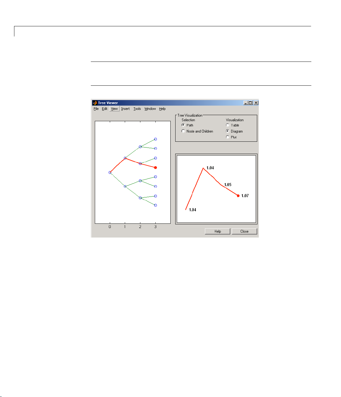
2 Using Financial Derivatives
Note If you are not familiar with the use of treeviewer, see the treeviewer
reference page for complete instructions on its use.
2-34

Pricing and Sensitivity from HJM
This section explains how to use the Financial Derivatives Toolbox to compute
prices and sensitivities of several financial instruments using the
Heath-Jarrow-Morton (HJM) model. For information, see:
• “Pricing and the Price Tree” on page 2-35 for a discussion of using the
hjmprice function to compute prices for a portfolio of instruments.
• “Calculating Prices and Sensitivities” on page 2-50 for a discussion of using
hjmsens function to compute delta, gamma, and vega portfolio
the
sensitivities.
Pricing and the Price Tree
For the HJM model, the function hjmprice calculates the price of any set of
supported instruments, based on an interest rate tree. The function is capable
of pricing these instrument types:
• Bonds
• Bond options
• Arbitrary cash flows
• Fixed-rate notes
• Floating-rate notes
• Caps
• Floors
• Swaps
Pricing and Sensitivity from HJM
The syntax used for calling
[Price, PriceTree] = hjmprice(HJMTree, InstSet, Options)
This function requires two input arguments: the interest rate tree, HJMTree,
and the set of instruments,
controls the pricing and the output displayed.
HJMTree is the Heath-Jarrow-Morton tree sampling of a forward rate process,
created using
to learn how to create this structure.
hjmtree. See “Building an HJM Forward Rate Tree” on page 2-22
hjmprice is
InstSet. An optional argument Options further
2-35

2 Using Financial Derivatives
InstSet is the set of instruments to be priced. This structure represents the set
of instruments to be priced independently using the HJM model. The section
“Creating and Managing Instrument Portfolios” on page 1-6 explains how to
create this variable.
Options is an options structure created with the function derivset. This
structure defines how the HJM tree is used to find the price of instruments in
the portfolio, and how much additional information is displayed in the
command window when calling the pricing function. If this input argument is
not specified in the call to
hjmprice classifies the instruments and calls the appropriate pricing function
for each one of the instrument types. The pricing functions are
cfbyhjm, fixedbyhjm, floatbyhjm, optbndbyhjm, and swapbyhjm. You can also
hjmprice, a default Options structure is used.
bondbyhjm,
use these functions directly to calculate the price of sets of instruments of the
same type. See the documentation for these individual functions for further
information.
Example: HJM Pricing
Consider the following example, which uses the portfolio and interest rate data
in the MAT-file
MATLAB workspace.
deriv.mat included in the toolbox. Load the data into the
2-36
load deriv.mat
Use the MATLAB whos command to display a list of the variables loaded from
the MAT-file.
whos
Name Size Bytes Class
BDTInstSet 1x1 22708 struct array
BDTTree 1x1 5522 struct array
HJMInstSet 1x1 22700 struct array
HJMTree 1x1 6318 struct array
ZeroInstSet 1x1 14442 struct array
ZeroRateSpec 1x1 1580 struct array
HJMTree
hjmprice.
and HJMInstSet are the input arguments needed to call the function

Pricing and Sensitivity from HJM
Use the function instdisp to examine the set of instruments contained in the
variable
Index Type CouponRate Settle Maturity Period Basis ......... Name Quantity
1 Bond 0.04 01-Jan-2000 01-Jan-2003 1 NaN......... 4% bond 100
2 Bond 0.04 01-Jan-2000 01-Jan-2004 2 NaN......... 4% bond 50
Index Type UnderInd OptSpec Strike ExerciseDates AmericanOpt Name Quantity
3 OptBond 2 call 101 01-Jan-2003 NaN Option 101 -50
Index Type CouponRate Settle Maturity FixedReset Basis Principal Name Quantity
4 Fixed 0.04 01-Jan-2000 01-Jan-2003 1 NaN NaN 4% Fixed 80
Index Type Spread Settle Maturity FloatReset Basis Principal Name Quantity
5 Float 20 01-Jan-2000 01-Jan-2003 1 NaN NaN 20BP Float 8
Index Type Strike Settle Maturity CapReset Basis Principal Name Quantity
6 Cap 0.03 01-Jan-2000 01-Jan-2004 1 NaN NaN 3% Cap 30
Index Type Strike Settle Maturity FloorReset Basis Principal Name Quantity
7 Floor 0.03 01-Jan-2000 01-Jan-2004 1 NaN NaN 3% Floor 40
Index Type LegRate Settle Maturity LegReset Basis Principal LegType Name Quantity
8 Swap [0.06 20] 01-Jan-2000 01-Jan-2003 [1 1] NaN NaN [NaN] 6%/20BP Swap 10
HJMInstSet.
instdisp(HJMInstSet)
Note that there are eight instruments in this portfolio set: two bonds, one bond
option, one fixed rate note, one floating rate note, one cap, one floor, and one
swap. Each instrument has a corresponding index that identifies the
instrument prices in the price vector returned by
Now use
hjmprice to calculate the price of each instrument in the instrument
hjmprice.
set.
Price = hjmprice(HJMTree, HJMInstSet)
Warning: Not all cash flows are aligned with the tree. Result will
be approximated.
Price =
98.7159
97.5280
0.0486
98.7159
2-37

2 Using Financial Derivatives
100.5529
6.2831
0.0486
3.6923
Note The warning shown above appears because some of the cash flows for
the second bond do not fall exactly on a tree node. This situation is discussed
further in “HJM Pricing Options Structure” on page 2-44.
Price Vector
The prices in the output vector Price correspond to the prices at observation
time zero
rate tree. The instrument indexing within
within
the instruments in the following order.
InstNames = instget(HJMInstSet, 'FieldName','Name')
(tObs = 0), which is defined as the valuation date of the interest
Price is the same as the indexing
InstSet. In this example, the prices in the Price vector correspond to
2-38
InstNames =
4% bond
4% bond
Option 101
4% Fixed
20BP Float
3% Cap
3% Floor
6%/20BP Swap
Consequently, in the Price vector, the fourth element, 98.7159, represents the
price of the fourth instrument (4% fixed-rate note); the sixth element,
6.2831,
represents the price of the sixth instrument (3% cap).
Price Tree Structure
If you call the hjmprice function with two output arguments, e.g.,
[Price, PriceTree] = hjmprice(HJMTree, HJMInstSet)
you generate a price tree along with the price information.

Pricing and Sensitivity from HJM
The optional output price tree structure PriceTree holds all the pricing
information. The first field of this structure,
structure represents a price tree. The second field,
price of the instruments in each node of the tree. The third field,
FinObj, indicates that this
PBush is the tree holding the
AIBush is the
tree holding the accrued interest of the instruments in each node of the tree.
Finally, the fourth field,
PBush and AIBush, with units in terms of compounding periods.
tObs, represents the observation time of each level of
In this example the price tree looks like
PriceTree =
FinObj: 'HJMPriceTree'
PBush: {[8x1 double] [8x1x2 double] ...[8x8 double]}
AIBush: {[8x1 double] [8x1x2 double] ... [8x8 double]}
tObs: [0 1 2 3 4]
Both PBush and AIBush are actually 1-by-5 cell arrays, consistent with the five
observation times of
tObs. The data display has been shortened here to fit on a
single line.
Using the command line interface, you can directly examine
the field within the
PriceTree structure that contains the price tree with the
price vectors at every state. The first node represents
PriceTree.PBush,
tObs = 0, corresponding
to the valuation date.
PriceTree.PBush{1}
ans =
98.7159
97.5280
0.0486
98.7159
100.5529
6.2831
0.0486
3.6923
With this interface you can observe the prices for all instruments in the
portfolio at a specific time.
2-39

2 Using Financial Derivatives
Using treeviewer to View Instrument Prices Through Time
You can use the function treeviewer to display a graphical representation of
the tree, allowing you to examine interactively the prices on the nodes of the
tree until maturity. With
in the instrument portfolio for display. For example, the command
treeviewer(PriceTree, HJMInstSet)
with the 4% bond instrument selected in the Instrument window shows prices
for this bond instrument along the price tree from the valuation date until
maturity.
treeviewer you select each instrument individually
2-40
Example: Valuation Date Prices
You can use treeviewer instrument-by-instrument to observe instrument
prices through time. For the first 4% bond in the instrument portfolio,
treeviewer indicates a valuation date price of 98.72, the same value obtained
by accessing the
PriceTree structure directly.

Pricing and Sensitivity from HJM
As a further example, look at the sixth instrument in the price vector, the 3%
cap. At the valuation date its value obtained directly from the structure is
6.2831. Use
treeviewer on this instrument to confirm this price.
2-41

2 Using Financial Derivatives
2-42
Example: Additional Observation Times
The second node represents the first rate observation time, tObs = 1. This node
displays two states, one representing the branch going up and the other one
representing the branch going down.
Examine the prices of the node corresponding to the up branch.
PriceTree.PBush{2}(:,:,1)
ans =
100.1563
99.7309
0.1007
100.1563
100.3782
3.2594
0.1007
3.5597

Pricing and Sensitivity from HJM
As before, you can use treeviewer, this time to examine the price for the 4%
bond on the up branch.
treeviewer displays a price of 100.2 for the first node
of the up branch, as expected.
Now examine the corresponding down branch.
PriceTree.PBush{2}(:,:,2)
ans =
96.3041
94.1986
0
96.3041
100.3671
8.6342
0
-0.3923
Use treeviewer once again, now to observe the price of the 4% bond on the
down branch. The displayed price of 96.3 conforms to the price obtained from
2-43

2 Using Financial Derivatives
direct access of the PriceTree structure. You may continue this process as far
along the price tree as you want.
2-44
HJM Pricing Options Structure
The MATLAB structure Options provides additional input to each pricing
function. The
• Tells pricing functions how to use the interest rate tree to calculate
instrument prices
• Determines what additional information the command window displays
along with instrument prices.
You provide pricing options in an optional
pricing function. (See, for example,
Default Structure
If you do not specify the Options argument in the call to a pricing function, the
function uses a default structure. To observe the default structure, use
derivset without any arguments.
Options structure
Options argument passed to each
bondbyhjm or hjmprice.)

Pricing and Sensitivity from HJM
Options = derivset
Options =
Diagnostics: 'off'
Warnings: 'on'
ConstRate: 'on'
The Options structure has three fields: Diagnostics, Warnings, and
ConstRate.
Diagnostics indicates whether additional information is displayed if the HJM
tree is modified. The default value for this option is
set to
'on' and ConstRate is set to 'off', the pricing functions display
'off'. If Diagnostics is
information such as the number of nodes in the last level of the HJM tree
generated for pricing purposes.
Warnings indicates whether to display warning messages when the input tree
is not adequate for accurately pricing the instruments. The default value for
this option is
'on'. If both ConstRate and Warnings are 'on', a warning is
displayed if any of the instruments in the input portfolio has a cash flow date
between tree dates. If
ConstRate is 'off', and Warnings is 'on', a warning is
displayed if the tree is modified to match the cash flow dates on the
instruments in the portfolio.
ConstRate indicates whether the interest rates should be assumed constant
between tree dates. By default this option is
'on', which is not an
arbitrage-free assumption. Consequently the pricing functions return an
approximate price for instruments featuring cash flows between tree dates.
Instruments featuring cash flows only on tree nodes are not affected by this
option and return exact (arbitrage-free) prices. When
ConstRate is 'off', the
HJM pricing function finds the cash flow dates for all instruments in the
portfolio. If these cash flows do not align exactly with the tree dates, a new tree
is generated and used for pricing. This new tree features the same volatility
and initial rate specifications of the input HJM tree but contains tree nodes for
each date in which at least one instrument in the portfolio has a cash flow.
Keep in mind that the number of nodes in an HJM tree grows exponentially
with the number of tree dates. Consequently, setting
ConstRate 'off'
dramatically increases the memory and CPU demands on the computer.
2-45

2 Using Financial Derivatives
Customizing the Structure
Customize the Options structure by passing property name/property value
pairs to the
derivset function.
As an example, consider an
Diagonistics 'on'.
Options = derivset('ConstRate', 'off', 'Diagnostics', 'on')
Options =
Diagnostics: 'on'
Warnings: 'on'
ConstRate: 'off'
Options structure with ConstRate 'off' and
To obtain the value of a specific property from the Options structure, use
derivget.
CR = derivget(Options, 'ConstRate')
CR =
Off
Note Use derivset and derivget to construct the Options structure. These
functions are guaranteed to remain unchanged, while the implementation of
the structure itself may be modified in the future.
Now observe the effects of setting
ConstRate 'off'. Obtain the tree dates from
the HJM tree.
2-46
TreeDates = [HJMTree.TimeSpec.ValuationDate;...
HJMTree.TimeSpec.Maturity]
TreeDates =
730486
730852
731217
731582
731947

Pricing and Sensitivity from HJM
datedisp(TreeDates)
01-Jan-2000
01-Jan-2001
01-Jan-2002
01-Jan-2003
01-Jan-2004
All instruments in HJMInstSet settle on Jan 1st, 2000, and all have cash flows
once a year, with the exception of the second bond, which features a period of
2. This bond has cash flows twice a year, with every other cash flow
consequently falling between tree dates. You can extract this bond from the
portfolio to compare how its price differs by setting
'off'.
BondPort = instselect(HJMInstSet, 'Index', 2);
instdisp(BondPort)
Index Type CouponRate Settle Maturity Period Basis...
1 Bond 0.04 01-Jan-2000 01-Jan-2004 2 NaN...
ConstRate to 'on' and
First price the bond with ConstRate 'on' (default).
format long
[BondPrice, BondPriceTree] = hjmprice(HJMTree, BondPort)
Warning: Not all cash flows are aligned with the tree. Result will
be approximated.
BondPrice =
97.52801411736377
BondPriceTree =
FinObj: 'HJMPriceTree'
PBush: {1x5 cell}
AIBush: {[0] [1x1x2 double] ... [1x4x2 double] [1x8 double]}
tObs: [0 1 2 3 4]
Now recalculate the price of the bond setting ConstRate 'off'.
2-47

2 Using Financial Derivatives
OptionsNoCR = derivset('ConstR', 'off')
OptionsNoCR =
Diagnostics: 'off'
Warnings: 'on'
ConstRate: 'off'
[BondPriceNoCR, BondPriceTreeNoCR] = hjmprice(HJMTree,...
BondPort, OptionsNoCR)
Warning: Not all cash flows are aligned with the tree. Rebuilding
tree.
BondPriceNoCR =
97.53342361674437
BondPriceTreeNoCR =
FinObj: 'HJMPriceTree'
PBush: {1x9 cell}
AIBush: {1x9 cell}
tObs: [0 0.5000 1 1.5000 2 2.5000 3 3.5000 4]
2-48
As indicated in the last warning, because the cash flows of the bond did not
align with the tree dates, a new tree was generated for pricing the bond. This
pricing method returns more accurate results since it guarantees that the
process is arbitrage-free. It also takes longer to calculate and requires more
memory. The
memory usage.
BondPriceTreeNoCR.tObs has nine. While this may not seem like a large
tObs field of the price tree structure indicates the increased
BondPriceTree.tObs has only five elements, while
difference, it has a dramatic effect on the number of states in the last node.
size(BondPriceTree.PBush{end})
ans =
1 8
size(BondPriceTreeNoCR.PBush{end})

Pricing and Sensitivity from HJM
ans =
1 128
The differences become more obvious by examining the price trees with
treeviewer.
treeviewer(BondPriceTree, BondPort)
2-49

2 Using Financial Derivatives
treeviewer(BondPriceTreeNoCR, BondPort)
2-50
Calculating Prices and Sensitivities
The function hjmsens computes the delta, gamma, and vega sensitivities of
instruments using an interest rate tree created with
returns the calculated price for each instrument.
two input arguments used by
hjmsens calculates the dollar value of delta and gamma by shifting the
observed forward yield curve by 100 basis points in each direction, and the
dollar value of vega by shifting the volatility process by 1%. To obtain the
per-dollar value of the sensitivities, divide the dollar sensitivity by the price of
the corresponding instrument.
The calling syntax for the function is
[Delta, Gamma, Vega, Price] = hjmsens(HJMTree, HJMInstSet)
hjmprice, namely HJMTree and HJMInstSet.
hjmtree. It also optionally
hjmsens requires the same

Pricing and Sensitivity from HJM
Use the previous example data to calculate the price of instruments.
load deriv.mat
[Delta, Gamma, Vega, Price] = hjmsens(HJMTree, HJMInstSet);
Warning: Not all cash flows are aligned with the tree. Result will
be approximated.
Note The warning appears because some of the cash flows for the second
bond do not fall exactly on a tree node. This situation was discussed in “HJM
Pricing Options Structure” on page 2-44.
You can conveniently examine the sensitivities and the prices by arranging
them into a single matrix.
All = [Delta, Gamma, Vega, Price]
All =
-272.65 1029.90 0.00 98.72
-347.43 1622.69 -0.04 97.53
-8.08 643.40 34.07 0.05
-272.65 1029.90 0.00 98.72
-1.04 3.31 0 100.55
294.97 6852.56 93.69 6.28
-47.16 8459.99 93.69 0.05
-282.05 1059.68 0.00 3.69
As with the prices, each row of the sensitivity vectors corresponds to the
similarly indexed instrument in
HJMInstSet. To view the per-dollar
sensitivities, divide each dollar sensitivity by the corresponding instrument
price.
2-51

2 Using Financial Derivatives
All = [Delta ./ Price, Gamma ./ Price, Vega ./ Price, Price]
All =
-2.76 10.43 0.00 98.72
-3.56 16.64 -0.00 97.53
-166.18 13235.59 700.96 0.05
-2.76 10.43 0.00 98.72
-0.01 0.03 0 100.55
46.95 1090.63 14.91 6.28
-969.85 173969.77 1926.72 0.05
-76.39 287.00 0.00 3.690
2-52

Black-Derman-Toy Model (BDT)
The Black-Derman-Toy (BDT) model is an analytical model used for pricing
interest rate derivatives. The model considers a given initial zero rate term
structure of interest rates and a specification of the yield volatilities of long
rates to build a tree representing the evolution of the interest rates. For further
explanation, see the paper “A One Factor Model of Interest Rates and its
Application to Treasury Bond Options” by Fischer Black, Emanuel Derman,
and William Toy.
Building a BDT Interest Rate Tree
The BDT interest rate tree represents the evolution of interest rates in a given
period of time. This section explains how to create the BDT interest rate tree
using the Financial Derivatives Toolbox.
The MATLAB function that creates the BDT interest rate tree is bdttree. This
function takes three structures as input arguments:
Black-Derman-Toy Model (BDT)
• The volatility model
page 2-54.)
• The interest rate term structure
Rate Term Structure (RateSpec)” on page 2-55.)
• The tree time layout
(TimeSpec)” on page 2-56.)
VolSpec. (See “Specifying the Volatility (VolSpec)” on
RateSpec. (See “Specifying the Interest
TimeSpec. (See “Specifying the Time Structure
Creating the BDT Interest Rate Tree (bdttree)
Calling the function bdttree creates the structure, BDTTree, containing time
and interest rate information of the recombining tree.
This structure is a self-contained unit that includes the BDT tree of rates
(found in the
used in building this tree.
The calling syntax for
BDTTree = bdttree(VolSpec, RateSpec, TimeSpec)
where:
• VolSpec is a structure that specifies the interest rate volatility process.
VolSpec is created using the function bdtvolspec.
FwdTree field), and the volatility, rate, and time specifications
bdttree is
2-53

2 Using Financial Derivatives
• RateSpec is the interest rate specification of the initial rate curve. This
structure is created with the function
intenvset. (See “Interest Rate Term
Structure” on page 2-12.)
•
TimeSpec is the tree time layout specification. This variable is created with
the function
bdttimespec. It represents the mapping between level times
and level dates for rate quoting. This structure determines indirectly the
number of levels of the tree generated in the call to
bdttree.
Specifying the Volatility (VolSpec)
The function bdtvolspec generates the structure VolSpec, which specifies the
volatility process. The function requires three input arguments:
• The valuation date
• The yield volatility end dates
ValuationDate
VolDates
• The yield volatility values VolCurve
An optional fourth argument InterpMethod, specifying the interpolation
method, can be included.
The syntax used for calling
VolSpec = bdtvolspec(ValuationDate, VolDates, VolCurve,...
InterpMethod)
bdtvolspec is
where:
•
ValuationDate is the first observation date in the tree.
•
VolDates is a vector of dates representing yield volatility end dates.
•
VolCurve is a vector of yield volatility values.
•
InterpMethod is the method of interpolation to use. The default is 'linear'.
Consider the example
ValuationDate = datenum('01-01-2000');
EndDates = datenum(['01-01-2001'; '01-01-2002'; '01-01-2003';
'01-01-2004'; '01-01-2005']);
Volatility = [.2; .19; .18; .17; .16];
2-54
Use bdtvolspec to create a volatility specification. Because no interpolation
method is explicitly specified, the function uses the
'linear' default.

Black-Derman-Toy Model (BDT)
BDTVolSpec = bdtvolspec(ValuationDate, EndDates, Volatility)
BDTVolSpec =
FinObj: 'BDTVolSpec'
ValuationDate: 730486
VolDates: [5x1 double]
VolCurve: [5x1 double]
VolInterpMethod: 'linear'
Specifying the Interest Rate Term Structure (RateSpec)
The structure RateSpec is an interest term structure that defines the initial
interest rate specification from which the tree rates are derived. The section
“Interest Rate Term Structure” on page 2-12 explains how to create these
structures using the function
and ending dates for each rate, and the compounding value.
Consider the example
Compounding = 1;
Rates = [0.02; 0.02; 0.02; 0.02];
StartDates = ['01-Jan-2000';
'01-Jan-2001';
'01-Jan-2002';
'01-Jan-2003'];
EndDates = ['01-Jan-2001';
'01-Jan-2002';
'01-Jan-2003';
'01-Jan-2004'];
ValuationDate = '01-Jan-2000';
intenvset, given the interest rates, the starting
RateSpec = intenvset('Compounding',1,'Rates', Rates,...
'StartDates', StartDates, 'EndDates', EndDates,...
'ValuationDate', ValuationDate)
RateSpec =
FinObj: 'RateSpec'
Compounding: 1
Disc: [4x1 double]
Rates: [4x1 double]
2-55

2 Using Financial Derivatives
EndTimes: [4x1 double]
StartTimes: [4x1 double]
EndDates: [4x1 double]
StartDates: [4x1 double]
ValuationDate: 730486
Basis: 0
EndMonthRule: 1
Use the function datedisp to examine the dates defined in the variable
RateSpec. For example,
datedisp(RateSpec.ValuationDate)
01-Jan-2000
Specifying the Time Structure (TimeSpec)
The structure TimeSpec specifies the time structure for a BDT tree. This
structure defines the mapping between the observation times at each level of
the tree and the corresponding dates.
TimeSpec is built using the function bdttimespec. The bdttimespec function
requires three input arguments:
2-56
• The valuation date
ValuationDate
• The maturity date Maturity
• The compounding rate
The syntax used for calling
TimeSpec = bdttimespec(ValuationDate, Maturity, Compounding)
Compounding
bdttimespec is
where:
•
ValuationDate is the first observation date in the tree.
•
Maturity is a vector of dates representing the cash flow dates of the tree. Any
instrument cash flows with these maturities fall on tree nodes.
•
Compounding is the frequency at which the rates are compounded when
annualized.
Calling
structure,
bdttimespec with the same data used to create the interest rate term
RateSpec builds the structure that specifies the time layout for the
tree.

Black-Derman-Toy Model (BDT)
Maturity = EndDates;
TimeSpec = bdttimespec(ValuationDate, Maturity, Compounding)
TimeSpec =
FinObj: 'BDTTimeSpec'
ValuationDate: 730486
Maturity: [4x1 double]
Compounding: 1
Basis: 0
EndMonthRule: 1
Note that the maturities specified when building TimeSpec do not have to
coincide with the
defines the time-date mapping of the BDT tree, the rates in
EndDates of the rate intervals in RateSpec. Since TimeSpec
RateSpec are
interpolated to obtain the initial rates with maturities equal to those found in
TimeSpec.
Example: Creating a BDT Tree
Use the previously computed values for VolSpec, RateSpec, and TimeSpec as
input to the function
bdttree to create a BDT Tree.
BDTTree = bdttree(BDTVolSpec, RateSpec, TimeSpec)
BDTTree =
FinObj: 'BDTFwdTree'
VolSpec: [1x1 struct]
TimeSpec: [1x1 struct]
RateSpec: [1x1 struct]
tObs: [0 1.00 2.00 3.00]
TFwd: {[4x1 double] [3x1 double] [2x1 double] [3.00]}
CFlowT: {[4x1 double] [3x1 double] [2x1 double] [4.00]}
FwdTree: {[1.02]
[1.02 1.02] [1.01 1.02 1.03] [1.01 1.02 1.02 1.03]}
2-57

2 Using Financial Derivatives
Using BDT Trees in MATLAB
When working with the BDT model, the Financial Derivatives Toolbox uses
trees to represent interest rates, prices, etc. At the highest level, these trees
contain several MATLAB structures. The structures encapsulate information
needed to interpret completely the information contained in a tree.
Because BDT trees are essentially MATLAB structures, you can examine their
contents manually, just as you can for HJM trees. Consider this example,
which uses the data in the MAT-file
Load the data into the MATLAB workspace.
load deriv.mat
Display the list of the variables loaded from the MAT-file.
whos
Name Size Bytes Class
BDTInstSet 1x1 22708 struct array
BDTTree 1x1 5522 struct array
HJMInstSet 1x1 22700 struct array
HJMTree 1x1 6318 struct array
ZeroInstSet 1x1 14442 struct array
ZeroRateSpec 1x1 1580 struct array
deriv.mat included in the toolbox.
2-58
Structure of a BDT Tree
You can now examine in some detail the contents of the BDTTree structure.
BDTTree
BDTTree =
FinObj: 'BDTFwdTree'
VolSpec: [1x1 struct]
TimeSpec: [1x1 struct]
RateSpec: [1x1 struct]
tObs: [0 1 2 3]
TFwd: {[4x1 double] [3x1 double] [2x1 double] [3]}
CFlowT: {[4x1 double] [3x1 double] [2x1 double] [4]}
FwdTree: {1x4 cell}

Black-Derman-Toy Model (BDT)
FwdTree contains the actual rate tree. It is represented in MATLAB as a cell
array with each cell array element containing a tree level.
The other fields contain other information relevant to interpreting the values
in
FwdTree. The most important of these are VolSpec, TimeSpec, and RateSpec,
which contain the volatility, rate structure, and time structure information
respectively.
Look at the
RateSpec structure used in generating this tree to see where these
values originate. Arrange the values in a single array.
[BDTTree.RateSpec.StartTimes BDTTree.RateSpec.EndTimes...
BDTTree.RateSpec.Rates]
ans =
0 1.0000 0.1000
0 2.0000 0.1100
0 3.0000 0.1200
0 4.0000 0.1250
Note The Financial Derivatives Toolbox uses inverse discount notation for
forward rates in the tree. An inverse discount represents a factor by which the
present value of an asset is multiplied to find its future value. In general,
these forward factors are reciprocals of the discount factors.
Look at the rates in
tObs = 0. The second node represents tObs=1. Examine the rates at the
FwdTree. The first node represents the valuation date,
second, third and fourth nodes.
BDTTree.FwdTree{2}
ans =
1.0979 1.1432
The second node represents the first observation time, tObs = 1. This node
contains a total of two states, one representing the branch going up (
and the other representing the branch going down (
1.1432).
1.0979)
2-59

2 Using Financial Derivatives
Note The convention in this document is to display prices going up on the
upper branch. Consequently, when displaying rates, rates are falling on the
upper branch and increasing on the lower.
BDTTree.FwdTree{3}
ans =
1.0976 1.1377 1.1942
The third node represents the second observation time, tObs = 2. This node
contains a total of three states, one representing the branch going up (
one representing the branch in the middle (
the branch going down (
BDTTree.FwdTree{4}
ans =
1.1942).
1.1377) and the other representing
1.0976),
2-60
1.0872 1.1183 1.1606 1.2179
The fourth node represents the third observation time, tObs = 3. This node
contains a total of four states, one representing the branch going up (
two representing the branches in the middle (
representing the branch going down (
1.2179).
1.1183 and 1.1606) and the other
1.0872),
Verifying Results with treepath
The function treepath isolates a specific node by specifying the path to the
node as a vector of branches taken to reach that node. As an example, consider
the node reached by starting from the root node, taking the branch up, then the
branch down, and finally another branch down. Given that the tree has only
two branches per node, branches going up correspond to a 1, and branches
going down correspond to a 2. The path up-down-down becomes the vector
[122].

FRates = treepath(BDTTree.FwdTree, [1 2 2])
FRates =
1.1000
1.0979
1.1377
1.1606
Black-Derman-Toy Model (BDT)
treepath
returns the short rates for all the nodes touched by the path specified
in the input argument, the first one corresponding to the root node, and the last
one corresponding to the target node.
Graphical View of Interest Rate Tree
The function treeviewer provides a graphical view of the path of interest rates
specified in
treeviewer representation of the rates along several branches of BDTTree.
treeviewer(BDTTree)
BDTTree. For example, load the file deriv.mat. Here is a
2-61
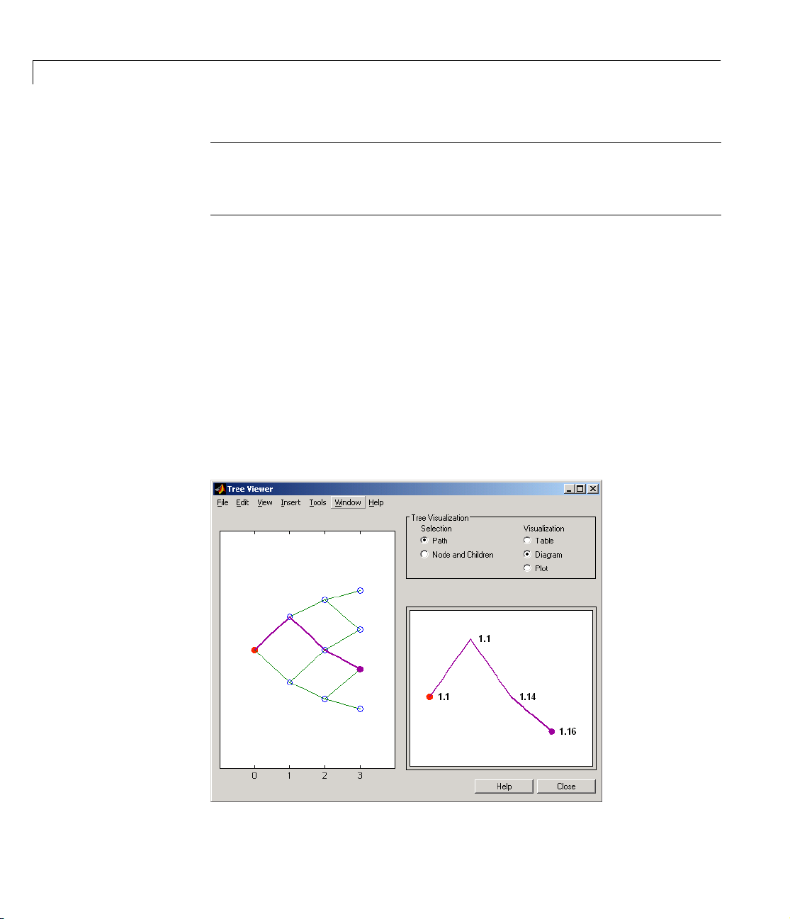
2 Using Financial Derivatives
Note When using treeviewer with BDT trees, you must click on each node in
succession from the beginning to the end. Because BDT trees can recombine,
treeviewer is unable to compute the path automatically.
A previous example used
treepath to find the path of interest rates taking the
first branch up and then two branches down the rate tree.
FRates = treepath(BDTTree.FwdTree, [1 2 2])
FRates =
1.1000
1.0979
1.1377
1.1606
The treeviewer function displays the same information obtained by clicking
along the sequence of nodes, as shown next.
2-62

Pricing and Sensitivity from BDT
This section explains how to use the Financial Derivatives Toolbox to compute
prices and sensitivities of several financial instruments using the
Black-Derman-Toy (BDT) model. For information, see:
• “Pricing and the Price Tree” on page 2-63 for a discussion of using the
bdtprice function to compute prices for a portfolio of instruments.
• “Calculating Prices and Sensitivities” on page 2-71 for a discussion of using
bdtsens function to compute delta, gamma, and vega portfolio
the
sensitivities.
Pricing and the Price Tree
For the BDT model, the function bdtprice calculates the price of any set of
supported instruments, based on an interest rate tree. The function is capable
of pricing these instrument types:
• Bonds
• Bond options
• Arbitrary cash flows
• Fixed-rate notes
• Floating-rate notes
• Caps
• Floors
• Swaps
Pricing and Sensitivity from BDT
The syntax used for calling
[Price, PriceTree] = bdtprice(BDTTree, InstSet, Options)
This function requires two input arguments: the interest rate tree, BDTTree,
and the set of instruments,
controls the pricing and the output displayed.
BDTTree is the Black-Derman-Toy tree sampling of an interest rate process,
created using
to learn how to create this structure based on the volatility model, the interest
rate term structure, and the time layout.
bdttree. See “Building a BDT Interest Rate Tree” on page 2-53
bdtprice is
InstSet. An optional argument Options further
2-63

2 Using Financial Derivatives
InstSet is the set of instruments to be priced. This structure represents the set
of instruments to be priced independently using the BDT model. The section
“Creating and Managing Instrument Portfolios” on page 1-6 explains how to
create this variable.
Options is an options structure created with the function derivset. This
structure defines how the BDT tree is used to find the price of instruments in
the portfolio, and how much additional information is displayed in the
command window when calling the pricing function. If this input argument is
not specified in the call to
bdtprice classifies the instruments and calls appropriate pricing function for
each of the instrument types. The pricing functions are
fixedbybdt, floatbybdt, optbndbybdt, and swapbybdt. You can also use these
bdtprice, a default Options structure is used.
bondbybdt, cfbybdt,
functions directly to calculate the price of sets of instruments of the same type.
See the documentation for these individual functions for further information.
BDT Pricing Example
Consider the following example, which uses the data in the MAT-file
deriv.mat included in the toolbox. Load the data into the MATLAB workspace.
2-64
load deriv.mat
Use the MATLAB whos command to display a list of the variables loaded from
the MAT-file.
whos
Name Size Bytes Class
BDTInstSet 1x1 22708 struct array
BDTTree 1x1 5522 struct array
HJMInstSet 1x1 22700 struct array
HJMTree 1x1 6318 struct array
ZeroInstSet 1x1 14442 struct array
ZeroRateSpec 1x1 1580 struct array
BDTTree
bdtprice.
Use the function
variable
and BDTInstSet are the input arguments needed to call the function
instdisp to examine the set of instruments contained in the
BDTInstSet.

Pricing and Sensitivity from BDT
instdisp(BDTInstSet)
Index Type CouponRate Settle Maturity Period Basis ......... Name Quantity
1 Bond 0.1 01-Jan-2000 01-Jan-2003 1 NaN......... 10% bond 100
2 Bond 0.1 01-Jan-2000 01-Jan-2004 2 NaN......... 10% bond 50
Index Type UnderInd OptSpec Strike ExerciseDates AmericanOpt Name Quantity
3 OptBond 1 call 9501 Jan-2002 NaN Option 95 -50
Index Type CouponRate Settle Maturity FixedReset Basis Principal Name Quantity
4 Fixed 0.10 01-Jan-2000 01-Jan-2003 1 NaN NaN 10% Fixed 80
Index Type Spread Settle Maturity FloatReset Basis Principal Name Quantity
5 Float 20 01-Jan-2000 01-Jan-2003 1 NaN NaN 20BP Float 8
Index Type Strike Settle Maturity CapReset Basis Principal Name Quantity
6 Cap 0.15 01-Jan-2000 01-Jan-2004 1 NaN NaN 15% Cap 30
Index Type Strike Settle Maturity FloorReset Basis Principal Name Quantity
7 Floor 0.09 01-Jan-2000 01-Jan-2004 1 NaN NaN 9% Floor 40
Index Type LegRate Settle Maturity LegReset Basis Principal LegType Name Quantity
8 Swap [0.15 10] 01-Jan-2000 01-Jan-2003 [1 1] NaN NaN [NaN] 15%/10BP Swap 10
Note that there are eight instruments in this portfolio set: two bonds, one bond
option, one fixed rate note, one floating rate note, one cap, one floor, and one
swap. Each instrument has a corresponding index that identifies the
instrument prices in the price vector returned by
Now use
bdtprice to calculate the price of each instrument in the instrument
bdtprice.
set.
[Price, PriceTree] = bdtprice(BDTTree, BDTInstSet)
Warning: Not all cash flows are aligned with the tree. Result will
be approximated.
Price =
95.5030
93.9079
1.7657
95.5030
100.6054
1.4863
2-65

2 Using Financial Derivatives
0.0245
7.3032
Note The warning shown above appears because some of the cash flows for
the second bond do not fall exactly on a tree node. This situation is discussed
in “HJM Pricing Options Structure” on page 2-44.
Price Vector
The prices in the vector Price correspond to the prices at observation time zero
(tObs = 0), which is defined as the valuation date of the interest rate tree. The
instrument indexing within
In this example, the prices in the
in the following order.
InstNames = instget(BDTInstSet, 'FieldName','Name')
InstNames =
Price is the same as the indexing within InstSet.
Price vector correspond to the instruments
2-66
10% Bond
10% Bond
Option 95
10% Fixed
20BP Float
15% Cap
9% Floor
15%/10BP Swap
Consequently, in the Price vector, the fourth element, 95.5030, represents the
price of the fourth instrument (10% fixed-rate note); the sixth element,
1.4863,
represents the price of the sixth instrument (15% cap).
Price Tree Structure
The output price tree structure PriceTree holds all the pricing information.
The first field of this structure,
a price tree. The second field,
instruments in each node of the tree. The third field,
the accrued interest of the instruments in each node of the tree. The fourth
FinObj, indicates that this structure represents
PTree is the tree holding the price of the
AITree is the tree holding

Pricing and Sensitivity from BDT
field, tObs, represents the observation time of each level of PTree and AITree,
with units in terms of compounding periods.
The function
treeviewer provides a graphical representation of the tree,
allowing you to examine interactively the values on the nodes of the tree.
treeviewer(PriceTree, BDTInstSet)
Alternatively, you can directly examine the field within the PriceTree
structure, which contains the price tree with the price vectors at every state.
The first node represents
PriceTree.PTree{1}
ans =
95.5030
93.9079
1.7657
95.5030
100.6054
tObs = 0, corresponding to the valuation date.
2-67

2 Using Financial Derivatives
1.4863
0.0245
7.3032
You can also use treeviewer instrument-by-instrument to observe instrument
prices. For the first 10% bond in the instrument portfolio,
a valuation date price of
PriceTree structure directly.
95.5030, the same value obtained by accessing the
treeviewer indicates
2-68
The second node represents the first rate observation time,
tObs = 1. This
node displays two states, one representing the branch going up and the other
one representing the branch going down.
Examine the prices of the node corresponding to the up branch.

Pricing and Sensitivity from BDT
PriceTree.PTree{2}(:,1)
ans =
98.7816
97.9770
3.1458
98.7816
101.9562
0.5008
0.0540
5.6282
As before, you can use treeviewer, this time to examine the price for the 10%
bond on the up branch.
treeviewer displays a price of 98.7816 for the first
node of the up branch, as expected.
2-69
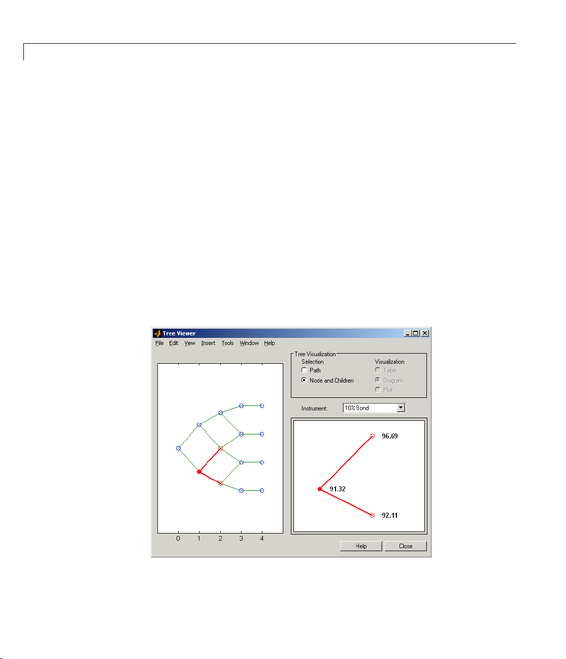
2 Using Financial Derivatives
Now examine the corresponding down branch.
PriceTree.PTree{2}(:,2)
ans =
91.3250
88.1322
0.7387
91.3250
98.9758
2.7691
0
0.6390
Use treeviewer once again, now to observe the price of the 10% bond on the
down branch. The displayed price of
from direct access of the
PriceTree structure. You may continue this process
91.3250 conforms to the price obtained
as far along the price tree as you want.
2-70
 Loading...