


Filter Design Tool
Getting Started Guide
box™ 4
How to Contact The MathWorks
www.mathworks.
comp.soft-sys.matlab Newsgroup
www.mathworks.com/contact_TS.html Technical Support
suggest@mathworks.com Product enhancement suggestions
bugs@mathwo
doc@mathworks.com Documentation error reports
service@mathworks.com Order status, license renewals, passcodes
info@mathwo
com
rks.com
rks.com
Web
Bug reports
Sales, prici
ng, and general information
508-647-7000 (Phone)
508-647-7001 (Fax)
The MathWorks, Inc.
3 Apple Hill Drive
Natick, MA 01760-2098
For contact information about worldwide offices, see the MathWorks Web site.
Filter Design Toolbox™ Getting Started Guide
© COPYRIGHT 2000–20 10 by The MathWorks, Inc.
The software described in this document is furnished under a license agreement. The software may be used
or copied only under the terms of the license agreement. No part of this manual may be photocopied or
reproduced in any form without prior written consent from The MathW orks, Inc.
FEDERAL ACQUISITION: This provision applies to all acquisitions of the Program and Documentation
by, for, or through the federal government of the United States. By accepting delivery of the Program
or Documentation, the government hereby agrees that this software or documentation qualifies as
commercial computer software or commercial computer software documentation as such terms are used
or defined in FAR 12.212, DFARS Part 227.72, and DFARS 252.227-7014. Accordingly, the terms and
conditions of this Agreement and only those rights specified in this Agreement, shall pertain to and govern
theuse,modification,reproduction,release,performance,display,anddisclosureoftheProgramand
Documentation by the federal government (or other entity acquiring for or through the federal government)
and shall supersede any conflicting contractual terms or conditions. If this License fails to meet the
government’s needs or is inconsistent in any respect with federal procurement law, the government agrees
to return the Program and Docu mentation, unused, to The MathWorks, Inc.
Trademarks
MATLAB and Simulink are registered trademarks of The MathWorks, Inc. See
www.mathworks.com/trademarks for a list of additional trademarks. Other product or brand
names may be trademarks or registered trademarks of their respective holders.
Patents
The MathWorks products are protected by one or more U.S. patents. Please see
www.mathworks.com/patents for more information.

Revision History
March 2007 Online only Revised for Version 4.1 (Release 2007a)
September 2007 Online only Revised for Version 4.2 (Release 2007b)
March 2008 Online only Revised for Version 4.3 (Release 2008a)
October 2008 Online only Revised for Version 4.4 (Release 2008b)
March 2009 Online only Revised for Version 4.5 (Release 2009a)
September 2009 Online only Revised for Version 4.6 (Release 2009b)
March 2010 Online only Revised for Version 4.7 (Release 2010a)


Product Overview
1
Introduction ...................................... 1-2
Contents
Uses with Othe
Key Features
Filter Des
r MathWorks Products
......................................
ign with Fdesign and Filterbuilder
...............
2
Filter Design Process Overview ..................... 2-2
Basic Filter Design Process
Using Filterbuild er to Design a Filter
......................... 2-4
............... 2-9
Designing Multirate and Multistage Filters
3
1-3
1-3
Multirate Filters ................................... 3-2
Why Are Multirate Filters Needed?
Overview of Multirate Filters
Multistage Filters
Why Are Multistage Filters Needed?
Optimal Multistage Filters in Filter Design Toolbox
Software
.................................. 3-6
....................................... 3-6
................... 3-2
........................ 3-2
.................. 3-6
v

Example Case for Multirate/Multistage Filters ....... 3-8
Example Overview
Single-Rate/Single-Stage Equiripple Design
Reducing Computational Cost Using Mulitrate/Multistage
Design
Comparing the Response
Further Performance Comparison
........................................ 3-9
................................ 3-8
............ 3-8
........................... 3-9
.................... 3-10
Converting from Floati ng-Point to Fixed-Point
4
Overview of Fixed-Point Filters ..................... 4-2
What Is a Fixed-Point Filter?
........................ 4-2
Floating-Point to Fixed-Point Conversion
Process Overview
Designing the Filter
Quantizing the Coefficients
Dynamic Range Analysis
Comparing Magnitude Response and Magnitude Response
Estimate
Data Types
Data Type Support
Fixed Data Type Support
Single Data Type Support
........................................ 4-11
................................. 4-3
............................... 4-3
......................... 4-4
........................... 4-7
...................................... 4-8
................................ 4-11
........................... 4-11
.......................... 4-11
............ 4-3
Designing Adaptive Filters
5
Adaptive Filters Tutorial ........................... 5-2
Signal Enhancement Example Overview
Create the Signals for Adaptation
Construct Two Adaptive Filters
Choose the Step Size
Set the Adapting Filter Step Size
............................... 5-4
.................... 5-2
...................... 5-3
..................... 5-5
.............. 5-2
vi Contents

Filter with the Adaptive Filters ...................... 5-5
Compute the Optimal Solution
Plot the Results
Compare the Final Coefficients
Reset the Filter Before Filtering
Investigate Convergence Through Learning Curves
Compute the Learning Curves
Compute the Theoretical Learning Curves
................................... 5-6
....................... 5-5
...................... 5-7
..................... 5-7
....................... 5-9
............. 5-10
Examples
A
Getting Started .................................... A-2
..... 5-8
Using Filterbuilder
................................ A-2
Index
vii

viii Contents

Product O verview
• “Introduction” on page 1-2
• “Uses with Other MathWorks Products” on page 1-3
• “Key Features” on page 1-3
1

1 Product Overview
Introduction
Filter Design Toolbox™ software is a collection of tools that provides
advanced techniques for designing, simulating, and analyzing digital
filters. It extends the capabilities of Signal Processing Toolbox™ software
with filter architectures and design methods for com plex real-time DSP
applications, including adaptive filtering and multirate filtering, as well as
filter transformations.
1-2

Uses with Other MathWorks Products
Used with Fixed-Point Toolbox™, Filter Design Toolbox software provides
functions that simplify the design of fixed-point filters and the analysis of
quantization effects. When used with Filter Design HDL Coder™ product,
Filter Design Toolbox software lets you generate VHDL and Verilog code
for fixed-point filters. Filter Design Toolbox software also brings advanced
filter design capabilities to Simulink
software.
®
and the Signal Processing Blockset™
Uses with Other MathWorks™ Products
Key Feature
s
• Advanced F
minimum-p
multistag
• Advanced
equalize
and comb f
• Multira
CIC comp
• Suppor
sectio
• Adapti
RLS-ba
proje
e, Farrow, and interpolated FIR
rs, parametric equalizers, octave, halfband, quasi-linear phase,
te filter design methods, including cascaded integrator-comb (CIC),
ensator, polyphase FIR and IIR, and multistage Nyquist filters
t for efficient IIR filter implementations, including second-order
ns and lattice wave digital filters
ve filter design, analysis, and implementation, including LMS-based,
sed, lattice-based, frequency-domain, fast transversal, and affine
ction
IR filter design methods, including minimum-order,
hase, shaped-stopband, halfband, complexity-optimized
IIR design methods, including arbitrary magnitude, group-delay
ilters
1-3

1 Product Overview
1-4

2
Filter Design with Fdesign
and Filterbuilder
• “Filter Design Process Overview” on page 2-2
• “Basic Filter Design Process” on page 2-4
• “Using Filterbuilder to Design a Filter” on page 2-9

2 Filter Design with Fdesign and Filterbuilder
Filter Design Process Overview
Note You must have the Signal Processing Toolbox installed to use fdesign
and fil terb uilder. A dvanced capabilities are available if your installation
additionally includes the Filter Design Toolbox license. You can verify the
presence of both toolboxes by typing
Filter design through user-defined specifications is the core of the fdesign
approach. This specification-centric approach places less emphasis on the
choice of specific filter algorithms, and more emphasis on performance during
the design a good working filter. For example, you can take a given set of
design parameters for the filter, such as a stopband frequency, a passband
frequency, and a stopband attenuation, and— using these parameters—
design a specification object for the filter. You can then implement the filter
using this specification object. Using this approach, it is also possible to
compare different algorithms as applied to a set of specifications.
ver at the command prompt.
2-2
There are two distinct objects involved in filter design:
• Specification Object — Captures the required design parameters of a filter
• Implementation Object — Describes the designed filter; includes the array
of coefficients and the filter structure
The distinction between these two objects is at the core of the filter design
methodology. The basic attributes of each of these objects are outlined in the
following table.
fication Objec t
Speci
-level specification
High
rithmic properties
Algo
You can run the code in the following examples from the Help browser (select
the code, right-click the selection, and choose Evaluate Selection from the
context menu), or you can enter the code on the MATLAB
Before you begin this example, start MATLAB and verify that you have
installed the Signal Processing Toolbox software. If you wish to access the
Implementation Object
er coefficients
Filt
Filter structure
®
command line.

Filter Design Process Overview
full functionality of fdesign and filterbuilder, you should additionally
obtain the Filter Des ign Toolbox software. You can verify the presence of
these products by typing
ver at the command prompt.
2-3

2 Filter Design with Fdesign and Filterbuilder
Basic Filter Design Process
Use the following two steps to design a simple filter.
1 Create a filter specification object.
2 Design your filter.
Example — Design a Filter in Two Steps
Assume that you want to design a bandpass filter. Typically a bandpass filter
is defined as shown in the following figure.
2-4
In this example, a sampling frequency of Fs = 48 kHz is used. This bandpass
filter has the following specifications, specified here using MATLAB code:
A_stop1 = 60; % Attenuation in the first stopband = 60 dB
F_stop1 = 8400; % Edge of the stopband = 8400 Hz
F_pass1 = 10800; % Edge of the passband = 10800 Hz
F_pass2 = 15600; % Closing edge of the passband = 15600 Hz
F_stop2 = 18000; % Edge of the second stopband = 18000 Hz
A_stop2 = 60; % Attenuation in the second stopband = 60 dB
A_pass = 1; % Amount of ripple allowed in the passband = 1 dB
In the followin g two steps, these spe c if ica t ion s are passed to the
fdesign.bandpass method as parameters.

Basic Filter Design Process
Step 1
To create a filter specification object, evaluate the following code at
the MATLAB prompt:
d = fdesign.bandpass
Now, pass the filter specifications that correspond to the default
Specification — fst1,fp1,fp2,fst2,ast1 ,ap,ast2.Thisexampleadds
fs as the final input argument to specify the sampling frequency of
48 kHz.
>> BandPassSpecObj = ...
fdesign.bandpass('Fst1,Fp1,Fp2,Fst2,Ast1,Ap,Ast2', ...
F_stop1, F_pass1, F_pass2, F_stop2, A_stop1, A _pas s, ...
A_stop2, 48000)
Note The order of the filter is not specified, allowing a degree of
freedom for the algorithm design in order to achieve the specification.
The design will be a minimum order design.
The specification parameters, such as Fstop1,areallgivendefault
values when none are provided. You can change the values of the
specification parameters after the filter specification object has been
created. For example, if there are two values that need to be changed,
Fpass2 and Fstop2,usetheset command, which takes the object first,
and then the parameter value pairs. Evaluate the following code at
the MATLAB prompt:
>> set(BandPassSpecObj, 'Fpass2', 15800, 'Fstop2', 18400)
BandPassSpecObj
is the new filter specification object which contains
all the required design parameters, including the filter type.
You may also change parameter values in filter specification objects by
accessing them as if they were elements in a
>> BandPassSpecObj.Fpass2=15800;
struct array.
2-5

2 Filter Design with Fdesign and Filterbuilder
Step 2
Design the filter by using the
design methods available for you specification object by calling the
designmethods function. For example, in this case, you can execute
the command
>> designmethods(BandPassSpecObj)
Design Methods for class
fdesign.bandpass (Fst1,Fp1,Fp2,Fst2,Ast1,Ap,Ast2):
butter
cheby1
cheby2
ellip
equiripple
kaiserwin
design command. You can access the
2-6
After choosing a design method use, you can evaluate the following at the
MATLAB prompt (this example assumes you’ve chosen ’
>> BandPassFilt = design( BandPassSpecObj, 'equiripple')
BandPassFilt =
FilterStructure: 'Direct-Form FIR'
Arithmetic: 'double'
Numerator: [1x44 double]
PersistentMemory: false
equiripple’):

Basic Filter Design Process
Note If you do not specify a design method, a default method will be
used. For example, you can execute the command
>> BandPassFilt = design( BandPassSpecObj)
BandPassFilt =
FilterStructure: 'Direct-Form FIR'
Arithmetic: 'double'
Numerator: [1x44 double]
PersistentMemory: false
and a design method will be selected automatically.
To check your work, you can plot the filter magnitude response using the
Filter Visualization tool. Verify that all the design parameters are met:
>> fvtool(BandPassFilt) %plot the fil ter magnitude response
If you have the Filter Design Toolbox installed, the Filter Visualization
tool produces the following figure with the dashed red lines indicating
the transition bands and unity gain (0 in dB) over the passband. If
you do not have the Filter Design Toolbox,thefigureappearswithout
the dashed red lines.
2-7

2 Filter Design with Fdesign and Filterbuilder
With only the Signal Processing Toolbox software installed:
2-8
Using Filterbuilder to Design a Filter
Filterbuilder presents the option of designing a filter using a GUI dialog box
as opposed to the command line instructions. You can use Filterbuilder to
design the same bandpass filter designed in the previous section, “Basic Filter
Design Process” on page 2-4
Example — Using Filterbuilder to Design a Simple Filter
To design the filter using FilterBuilder:
1 Type the following at the MATLA B prompt:
filterbuilder
The dialog box using the Filter Design Toolbox software appears a s follows:
Using Filterbuilder to Design a Filter
The dialog box using only the Signal Processing Toolbox software appears
as follows:
2-9

2 Filter Design with Fdesign and Filterbuilder
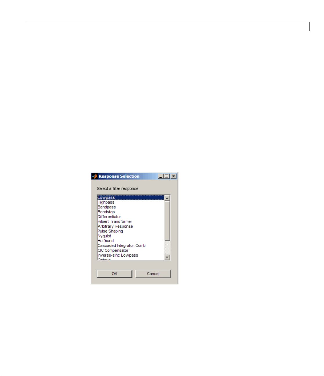
2 Select Bandpass filter response from the list in the dialog box, and hit the
OK button. The following dialog box opens:
2-10

Using Filterbuilder to Design a Filter
3 Enter the correct frequencies for Fpass2 and Fstop2,asshowninthe
preceding figure, then click OK. Here the specification uses normalized
frequency, so that the passband and stopband edges are expressed as a
fraction of the Nyquist frequency (in this case, 48/2 kHz). The following
message appears at the MATLAB prompt:
The variable 'Hbp' has be en exported to the command window.
IfyoudisplaytheWorkspacetab,asshowninthefollowingfigure,yousee
the object
Hbp has been placed on your workspace.
2-11

2 Filter Design with Fdesign and Filterbuilder
4 To check your work, plot the filter magnitude response using the Filter
Visualization tool. Verify that all the design parameters are met:
fvtool(Hbp) %plot the fil ter magnitude response
2-12
Note that the dashed red line s on the preced ing figure will only appear if
you are using the Filter Design Toolbox software.

Designing Multirate and
Multistage Filters
• “Multirate Filters” on page 3-2
• “Multistage Filters” on page 3-6
• “Example Case for Multirate/Multistage Filters” on page 3-8
3

3 Designing Multirate and Multistage Filters
Multirate Filters
In this section...
“Why Are Multirate Filters Needed?” on page 3-2
“Overview of Multirate Filters” on page 3-2
Why Are Multirate Filters N eeded?
Multirate filters can bring efficiency to a particularfilterimplementation.
In general, multirate filters are filters in which different parts of the filter
operate at different rates. The most obvious application of such a filter is
when the input sample rate and output sample rate need to differ (decimation
or interpolation) — however, multirate filters are also often used in designs
where this is not the case. For example you may have a system where the
input sample rate and output sample rate are the same, but internally there
is decimation and interpolation occurring in a series of filters, such that the
final output of the system has the same sample rate as the input. Such a
design may exhibit lower cost than could be achieved with a single-rate filter
for various reasons. For more information about the relative cost benefit
of using multirate filters, refer to [2] Harris, Fredric J., Multirate Signal
Processing for Communication Systems, Prentice Hall PTR, 2004.
3-2
Overview of Multirate Filters
A filter that reduces the input rate is called a decimator.Afilterthat
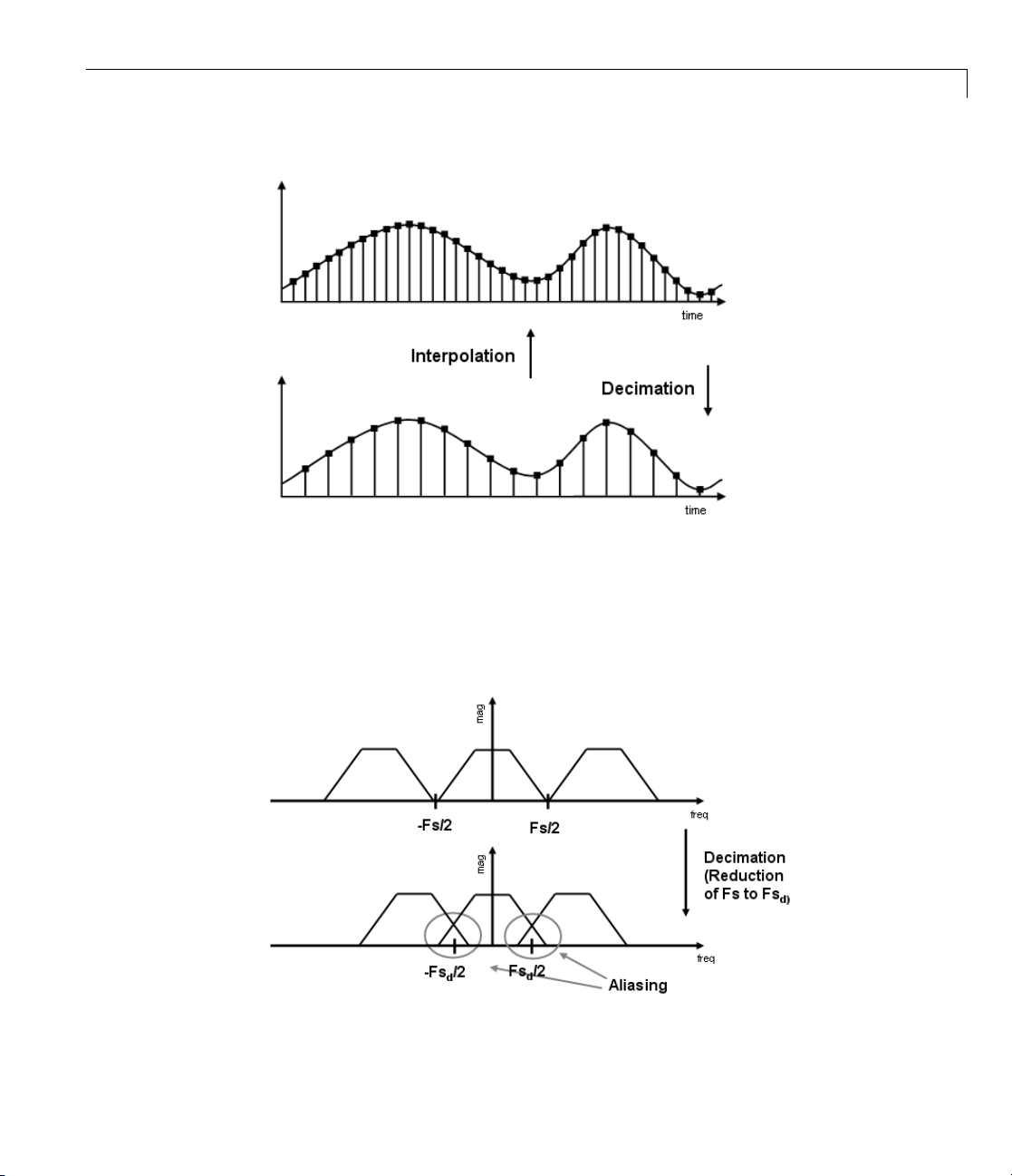
increases the input rate is called an interpolator. To visualize this process,
examine the following figure, which illustrates the processes of interpolation
and decimation in the time domain.
Multirate Filters
If you start with the top signal, sampled at a frequency Fs, then the bottom
signal is sampled at
is
2.
Fs/2 frequency. In this case, the decimation factor, or M,
The following figure illustrates effect of decimation in the frequency domain.
3-3

3 Designing Multirate and Multistage Filters
In the first graphic in the figure you can see a signal that is critically sampled,
i.e. thesamplerateisequaltotwotimesthehighestfrequencycomponent
of the sampled signal. As such the period of the signal in the frequency
domain is no greater than the bandwidth of the sampling frequency. When
reduce the sampling frequency (decimation), aliasing can occur, where the
magnitudes at the frequencies near the edges of the original period become
indistinguishable, and the information about these values becomes lost. To
work around this problem, the signal can be filtered before the decimation
process, avoiding overlap of the signal spectra at Fs/2.
3-4
An analogous approach must be taken to avoid imaging when performing
interpolation on a sampled signal. For more information about the effects of
decimation and interpolation on a sampled signal, refer to any one of the
references in the “Bibliography” section of the Filter Design Toolbox User
Guide.
The following list summarizes some guidelines and general requirements
regarding decimation and interpolation:
• By the Nyquist Theorem, for band-limited signals, the sampling frequency
must be at least twice the bandwidth of the signal. For example, if you
have a lowpass filter with the highest frequency of 10 MHz, and a sampling
frequency of 60 MHz, the highest frequency that can be handled by the
system without aliasing is 60/2=30, which is greater than 10. You could
safely set M=2 in this case, since (60/2)/2=1 5, which is sti ll greater than 10.
Multirate Filters
• If you wish to decimate a signal which does not meet the frequency criteria,
you can either:
- Interpolate first, and then decimate
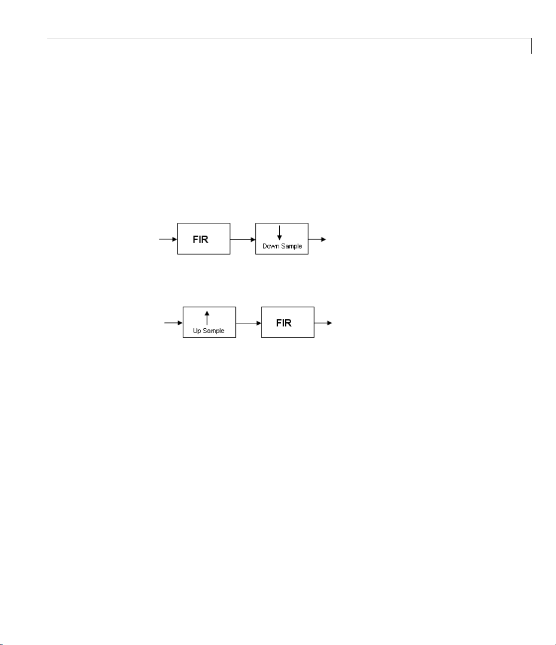
- When decimating, you should apply the filter first, then perform the
decimation. When interpolating a signal, you should interpolate first,
then filter the signal.
• Typically in dec im ation of a signal a filter is applied first, thereby allowing
decimation without aliasing, as shown in the following figure:
• Conversely, a filter is typically applied after interpolation to avoid imaging:
• M must be an integer. Although, if you wish to obtain an M of 4/5, you
could interpolate by 4, and then decimate by 5, provided that frequency
restrictions are met. This type of multirate filter will be referred to as a
sample rate converter in the documentation that follows.
Multirate filters are m ost often used in stages. This technique is introduced
in the following section.
3-5

3 Designing Multirate and Multistage Filters
Multistage Filters
In this section...
“Why Are Multistage Filters Needed?” on page 3-6
“Optimal Multistage Filters in Filter Design Toolb ox Software” on page 3-6
Why Are Multistage Filters Needed?
Typically used with multirate filters, multistage filters can bring efficiency
to a particular filter implementation. Multistage filters are composed of
several filters. These different parts of the mulitstage filter, called stages,are
connected in a cascade or in parallel. Howeversuchadesigncanconserve
resources in m any cases. There are many different uses for a multistage filter.
One of these is a filter requirement that includes a very narrow transition
width. For example, you need to design a lowpass filter w h ere the diffe rence
between the pass frequency and the stop frequency is .01 (normalized).
For such a requirement it is possible to design a single filter, but it will
be very long (containing many coefficients) and very costly (having many
multiplications and additions per input sample). Thus, this single filter
maybesocostlyandrequiresomuchmemory,thatitmaybeimpractical
to implement in certain applications where there are strict hardware
requirements. In such cases, a multistage filter is a great solution. Another
application of a multistage filter is for a mu litrate system, where there is a
decimatororaninterpolatorwithalarge factor. In these cases, it is usually
wise to break up the filter into several multirate stages, each comprising a
multiple of the total decimation/interpolation factor.
3-6
Optimal Multistage Filters in Filter Design Toolbox
Software
As described in the previous section, within a multirate filter each
interconnected filter is called a stage. While it is pos s ible to design
a multistage filter m anually, it is also possible to perform automatic
optimization of a multistage filter automatically. When designing a filter
manually it can be difficult to guess how many stages would provide an
optimal design, optimize each stage, and then optimize all the stages together.
Filter Design Toolbox software enables you to create a Specifications Object,
and then design a filter using multistage as an option. The rest of the work is

Multistage Filters
done automatically. Not only does Filter Design Toolbox software determine
the optimal number of stages, but it also optimizes the total filter solution.
3-7

3 Designing Multirate and Multistage Filters
Example Case for Multirate/Multistage Filters
In this section...
“Example Overview” o n page 3-8
“Single-Rate/Single-Stage Equiripple Design” on page 3-8
“Reducing Computational Cost Using Mulitrate/Multistage Design” on
page 3-9
“Comparing the Response” on page 3-9
“Further Performance Comparison” on page 3-10
Example Overview
This brief examp l e shows the efficiency gains that are possible when using
multirate and multistage filters for certain applications. In this case a distin c t
advantage is achieved over regular linear-phase equiripple design when a
narrow transition-band width is required. A more detailed treatment of the
keypointsmadeherecanbefoundinthedemoentitled“EfficientNarrow
Transition-Band FIR Filter Design”.
3-8
Single-Rate/Single-Stage Equiripple Design
Consider the following design specifications for a lowpass filter (where the
ripples are given in linear units):
Fpass = 0.13; % Passband edge
Fstop = 0.14; % Stopband edge
Rpass = 0.001; % Passb and ripple, 0.0174 dB peak to peak
Rstop = 0.0005; % Stopband ripple, 66.0206 dB minimum attenuation
Hf = fdesign.lowpass(Fpass,Fstop,Rpass,Rstop,'linear');
A regular linear-phase equiripple design using these specifications can be
designed by evaluating the following:
Hd = design(Hf,'equiripple');

Example Case for Multirate/Multistage Filters
When you determine the cost of this design, you can see that 695 multipliers
are required.
cost(Hd)
Reducing Computational Cost Using
Mulitrate/Multistage Design
The number of multipliers required by a filter using a single state,
single rate equiripple design is 694. This number can be reduced using
multirate/multistage techniques. In any single-rate design, the number
of multiplications required by each input sample is equal to the number
of non-zero multipliers in the implementation. However, by using a
multirate/multistage design, decimation and interpolation can be combined
to lessen the computation required. For decimators, the average number
of multiplications required per input sample is given by the number of
multipliers divided by the decimation factor.
Hd_multi = design(Hf,'multistage');
You can then view the cost o f the filter created using this design step, and you
can see that a significant cost advantage has been achieved.
cost(Hd_multi)
Comparing the Response
You can compare the responses of the equiripple design and this
multirate/multistage design using fvtool:
hfvt = fvtool(Hd,Hd_multi);
legend(hfvt,'Equiripple design', 'Multirate/multistage design')
3-9

3 Designing Multirate and Multistage Filters
3-10
Notice that the stopband attenuation for the multistage design is about twice
that of the other designs. This is because the decimators must attenuate
out-of-band components by 66 dB in order to avoid alias ing th at would violate
the specifications. Similarly, the interpolators must attenuate images by
66 dB. You can also see that the passband gain for this design is no longer
0 dB, because each interpolator has a nominal gain (in linea r units) equal
to its interpolation factor, and the total interpolation factor for the three
interpolators is 6.
Further Performance Comparison
You can check the performance of the multirate/multistage design b y plotting
the power spectral densities o f the input and the various outputs, and you can
see that the sinusoid at
design and the multirate/multistage design.
n = 0:1799;
x = sin(0.1*pi*n') + 2*sin(0.15*pi*n');
y = filter(Hd,x);
04. π
is attenuated comparably by both the equiripple

Example Case for Multirate/Multistage Filters
y_multi = filter(Hd_multi,x);
[Pxx,w] = periodogram(x);
Pyy = periodogram(y);
Pyy_multi = periodogram(y_multi);
plot(w/pi,10*log10([Pxx,Pyy,Pyy_multi]));
xlabel('Normalized Frequency (x\pi rad/sample)');
ylabel('Power density (dB/rad/sample)');
legend('Input signal PSD','Equiripple output PSD',...
'Multirate/multistage output PSD')
axis([0 1 -50 30])
grid on
3-11

3 Designing Multirate and Multistage Filters
3-12

Converting from
Floating-Point to
Fixed-Point
• “Overview of Fixed-Point Filters” on page 4-2
• “Floating-Point to Fixed-Point Conversion” on page 4-3
• “Data Types” on page 4-11
4

4 Converting from Floating-Point to Fixed-Point
Overview of Fixed-Point Filters
The most common use of fix ed-point filters is in the DSP chips, where the
data storage capabilities are limited, or embedded systems and devices where
low-power consumption is necessary. For example, the data input may come
froma12bitADC,thedatabusmaybe16bit,andthemultipliermayhave24
bits. Within these space constraints, Filter Design Toolbox software enables
you to desig n the best possible fix ed-point filter.
What Is a Fixed-Point Filter?
A fixed-point filter uses fixed-point arithmetic and is represented by an
equation with fixed-point coefficients. To learn about fixed-point math, see
“Fixed-Point Concepts” in “Fixed-Point Toolbox” documentation.
4-2

Floating-Point to Fixed-Point Conversion
In this section...
“Process Overview” on page 4-3
“Designing the Filter” on page 4-3
“Quantizing the Coefficients” on page 4-4
“Dynamic Range Analysis” on page 4-7
“Comparing Magnitude Response and Magnitude Response Estimate” on
page 4-8
Process Overview
The conversion from floating-point to fixed-point consists of two main parts:
quantizing the coefficients and performing the dynamic range analysis.
Quantizing the coefficients is a process of converting the coefficients to
fixed-point numbers. The dynamic range analysis is a process of fine tuning
the scaling of each node to ensure that the fraction lengths are set for full
input range coverage and maximum precision. The following steps describe
this conversion process.
Floating-Point to Fixed-Point Conversion
Designing the Filter
Start by designing a regular, floating-point, equiripple bandpass filter, as
shown in the following figure.
4-3
4 Converting from Floating-Point to Fixed-Point
where the passband is from .45 to .55 of normalized frequency, the am ount
of ripple acceptable in the passband is 1 dB, the first stopband is from 0 to
.35 (normaliz ed), the second stopband is from .65 to 1 (normalized), and both
stopbands provide 60 dB of attenuation.
4-4
To design this filter, evaluate the following code, or type it at the M ATLAB
command prompt:
f = fdesign.bandpass(.35,.45,.55,.65,60,1,60);
Hd = design(f, 'equiripple ');
fvtool(Hd)
ThelastlineofcodeinvokestheFilterVisualization Tool, which displays the
designed filter. You use
baseline and a starting point for the conversion.
Hd, which is a double, floating-point filter, both as the
Quantizing the Coefficients
The first step in quantizing the coefficientsistofindthevalidwordlength
for the coefficients. Here again, the hardware usually dictates the maximum
allowable setting. However, if this constraint is large enough, there is room
for some trial and error. Start with the coefficient word length of 8 and
determine if the resulting filter is sufficient for your needs.

Floating-Point to Fixed-Point Conversion
To set the coefficient word length of 8, ev aluate or type the following code
at the MATLAB command prompt:
Hf = Hd;
Hf.Arithmetic = 'fixed';
set(Hf, 'CoeffWordLength', 8);
fvtool(Hf)
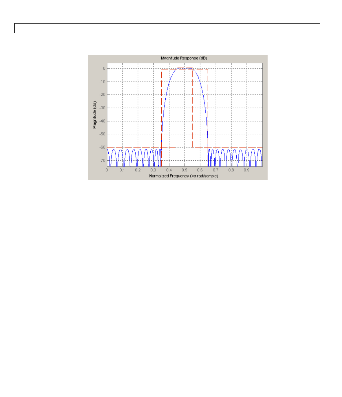
The resulting filter is shown in the following figure.
Asthefigureshows,thefilterdesignconstraints are not met. The attenuation
is not complete, and there is noise at the edges of the stopbands. You can
experiment with different coefficient word lengths if you like. For this
example, however, the word length of
To set the coefficient word length of
12 is sufficient.
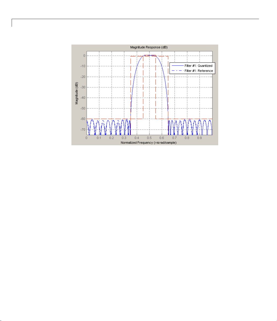
12, evaluate or type the following code
at the MATLAB command prompt:
set(Hf, 'CoeffWordLength', 12);
fvtool(Hf)
The resulting filter satisfies the design constraints, as shown in the following
figure.
4-5
4 Converting from Floating-Point to Fixed-Point
Now that the coe fficient word length is set, there are other data width
constraints that might require attention. Type the following at the MATLAB
command prompt:
4-6
>> info(Hf)
Discrete-Time FIR Filter ( real)
------------------------------Filter Structure : Direct-Form FIR
Filter Length : 48
Stable : Yes
Linear Phase : Yes (Type 2)
Arithmetic : fixed
Numerator : s12,14 -> [-1.250000e-0 01 1.250000e-001)
Input : s16,15 -> [-1 1)
Filter Internals : Full Precision
Output : s31,29 -> [-2 2) (auto determined)
Product : s27,29 -> [-1.250000e-0 01 1.250000e-001)...
(auto determined)
Accumulator : s31,29 -> [-2 2) (auto determined)
Round Mode : No rounding
Overflow Mode : No overflow

Floating-Point to Fixed-Point Conversion
You see the output is 31 bits, the accumulator requires 31 bits and the
multiplier requires 2 7 bits. A typical piece of hardware might have a 16 bit
data bus, a 24 bit multiplier, and an accumulator with 4 gua rd bits. A nother
reasonable assumption is that the data comes from a 12 bit ADC. To reflect
these constraints type or evaluate the following code:
set (Hf, 'InputWordLength', 12);
set (Hf, 'FilterInternals', 'SpecifyPrecision');
set (Hf, 'ProductWordLength', 24);
set (Hf, 'AccumWordLength', 28);
set (Hf, 'OutputWordLength', 16);
Although the filter is basically done, if you try to filter some data with it at
this stage, you may get erroneous resultsduetooverflows. Suchoverflows
occur because you have defined the constraints, but you have not tuned the
filter coefficients to handle properly the range of input data where the filter
is designed to operate. Next, the dynamic range analysis is necessary to
ensure no overflows.
Dynamic Range Analysis
Thepurposeofthedynamicrangeanalysisistofinetunethescalingofthe
coefficients. The ideal set of coefficients is valid for the full range of input
data, while the fraction lengths maximize precision. Consider carefully the
range of input data to use for this step. If you provide data that covers the
largest dynamic range in the filter, the resulting scaling is more conservative,
and some precision is lost. If you provide data that covers a very narrow
input range, the precision can be much greater, but an input out of the design
rangemayproduceanoverflow. Inthisexample, you use the worst-case input
signal, covering a full dynamic range, in order to ensure that no overflow
ever occurs. This worst-case input signal is a scaled version of the sign of
the flipped impulse response.
To scale the coefficients based on the full d y na m i c range, type or evaluate
the following code:
x = 1.9*sign(fliplr(impz(Hf)));
Hf = autoscale(Hf, x);
To check that the coefficients are in range (no overflows) and have maximum
possible precision, type or evaluate the following code:
4-7

4 Converting from Floating-Point to Fixed-Point
fipref('LoggingMode', 'on', 'DataTypeOverride', 'ForceOff');
y = filter(Hf, x);
fipref('LoggingMode', 'off');
R = qreport(Hf)
Where R is shown in the following figure:
4-8
The report shows no overflows, and all data falls within the designed range.
The conversion has completed successfully.
Comparing Magnitude Response and Magnitude
Response Estimate
You can use the fvtool GUI to do final analysis on your quantized filter,
to see the effects of the quantization on stopband attenuation, etc. Two
important last checks when analyzing a quantized filter are the Magnitude
Response Estimate and the Round-off Noise Power Spectrum. The value of the
Magnitude Response Estimate analysis can be seen in the following example.

Floating-Point to Fixed-Point Conversion
Viewing Magnitude Response Estimate
Begin by designing a simple lowpass filter using the command.
h = design(fdesign.lowpass, 'butter');
Now set the arithmetic to fixed-point.
h.arithmetic = 'fixed';
Open the filter using fvtool.
fvtool(h)
When fvtool displays the filter using the Magnitude response view, the
quantized filter seems to match the original filter quite well.
However if you look at the Magnitude Response Estimate plot from the
Analysis menu, you will see that the actual filter created may not perform
nearly as well as indicated by the Magnitude Response plot.
4-9

4 Converting from Floating-Point to Fixed-Point
4-10
This is because by using the noise-based method of the Magnitude Response
Estimate, you estimate the complex frequency response for your filter as
determined by applying a noise- like signal to the filter input. Magnitude
Response Estimate usestheMonteCarlotrialstogenerateanoisesignal
that contains complete frequency contentacrosstherange0toFs.Formore
information about analyzing filters in this way, refer to the section titled
Analyzing Filters with a Noise-Based Method in the User Guide.
For more information, refer to McClellan, et al., Computer-Based Ex ercises
for Signal Processing Using MATLAB 5, Prentice-Hall, 1998. See P roject 5:
Quantization Noise in Digital Filters, page 231.

Data Types
Data Types
In this section...
“Data Type Support” on page 4-11
“Fixed Data Type Support” on page 4-11
“SingleDataTypeSupport”onpage4-11
Data Type Support
There are three different data types supported in Filter Design Toolbox
software:
• Fixed — Requires Fixed Point Toolbox and is supported by packages listed
in “Fixed Data Type Support” on page 4-11.
• Double — Double precision, floating point and is the default data type for
Filter Design Toolbox software; accepted by all functions
• Single — Single precision, floating point and is supported by specific
packages outlined in “Single Data Type Support” on page 4-11.
FixedDataTypeSupport
To use fixed data type, you must have Fixed Point Toolbox. Type ver at the
MATLAB command prompt to get a listing of all installed products.
The fixed data type is reserved for any filter wh ose property
set to
fixed. Furthermore all functions that work with this filter, whether in
analysis or design, also accept and support the fixed data types.
To set the filter’s arithmetic property:
>> f = fdesign.bandpass(. 35,.45,.55,.65,60,1,60);
>> Hf = design(f, 'equiripple');
>> Hf.Arithmetic = 'fixed' ;
arithmetic is
Single Data Type Support
Thesupportofthesingledatatypescomes in two varieties. First, input data
of type single can be fed into a double filter, where it i s immediately converted
4-11

4 Converting from Floating-Point to Fixed-Point
to double. Thus, while the filter still operates in the double mode, the single
data type input does not break it. The second variety is where the filter itself
issettosingleprecision. Inthiscase,itacceptsonlysingledatatypeinput,
performs all calculations, and outputs data in single precision. Furthermore,
such analyses as
To set the filter to single precision:
>> f = fdesign.bandpass(. 35,.45,.55,.65,60,1,60);
>> Hf = design(f, 'equiripple');
>> Hf.Arithmetic = 'single ';
noisepsd and freqrespest also operate in single precision.
4-12

5
Designing Adaptive Filters

5 Designing Adaptive Filters
Adaptive Filters Tutorial
In this section...
“Signal Enhancement Example Overview” on page 5-2
“Create the Signals for Adaptation” on page 5-2
“Construct Two Adaptive Filters” on page 5-3
“Choose the Step Size” on page 5-4
“Set the Adapting Filter S tep Size” on page 5-5
“Filter with the Adaptive Filters” on page 5-5
“Compute the Optimal Solution” o n page 5-5
“Plot the Results” on page 5-6
“Compare the Final Coefficients” on page 5-7
“Reset the Filter BeforeFiltering”onpage5-7
“Investigate Convergence Through Learning Curves” on page 5-8
5-2
“Compute the Learning Curves” on page 5-9
“Compute the Theoretical Learning Curves” on page 5-10
Signal Enhancement Example Overview
This demonstration illustrates one way to use a few of the adaptive filter
algorithms provided in the toolbox. In this example, a signal enhancement
application is used as an illustration. While there are about 30 different
adaptive filtering algorithms included with the toolbox, this example
demonstrates two algorithms — least means square (LMS),
andnormalizedLMS,
adaptfilt.nlms, for adaptation.
adaptfilt.lms,
Create the Signals for Adaptation
The goal is to use an adaptive filter to extract a desired signal from a
noise-corrupted signal by filtering out the noise. The desired signal (the
output from the p rocess) is a sinusoid with 1000 samples.
n = (1:1000)';
s = sin(0.075*pi*n);

Adaptive Filters Tutorial
To perform adaptation requires two signals:
• a reference signal
• a noisy signal that contains both the desired signal and an added noise
component.
Generate the Noise Signal
To create a noise signal, assume that the noise v1 is autoregressive, meaning
that the value of the noise at time t depends only on its previous values and
on a random disturbance.
v = 0.8*randn(1000,1); % Random nois e part.
ar = [1,1/2]; % Autoregression coefficients.
v1 = filter(1,ar,v); % Noise signal . Applies a 1-D digital
% filter.
Corrupt the Desired Signal to Create a Noisy Signal
To generate the noisy signal that contains both the desired signal and the
noise, add the noise signal
sinusoid
x is
v1 to the desired signal s. The noise-corrupted
x=s+v1;
where s is the desired signal and the noise is v1. Adaptive filter processing
seeks to recover
s from x by removing v1. To complete the signals needed to
perform adaptive filtering, the adaptation process requires a reference signal.
Create a Reference Signal
Define a moving average signal v2 that is correlated with v1.Thisv2 is the
reference signal for the examples.
ma = [1, -0.8, 0.4 , -0.2];
v2 = filter(ma,1,v);
Construct Two Adaptive Filters
Two similar adaptive filters — LMS and NLMS — form the basis of this
example, both sixth order. Set the order as a variable in MATLAB and create
the filters.
5-3

5 Designing Adaptive Filters
L=7;
hlms = adaptfilt.lms(7);
hnlms = adaptfilt.nlms(7);
Choose the Step Size
LMS-like algorithms have a step size that determines the amount of
correction appl ie d as the filter adapts from one iteration to the next. Choosing
the appropriate step size is not always easy, usually requiring experience in
adaptive filter design.
• Astepsizethatistoosmallincreasesthetimeforthefiltertoconvergeon
a set of coefficients. This beco mes an issue of speed and accuracy.
• One that is too large may cause the adapting filter to diverge, never
reaching convergence. In this case, the issue is stability — the resulting
filter might not be stable.
As a rule of thumb, smaller step sizes improve the accuracy of the convergence
of the filter to match the characteristics of the unknown, at the expense of the
time it takes to adapt.
5-4
The toolbox includes an algorithm —
maxstep — to determine the maximum
step size suitable for each LMS adaptive filter algorithm that still ensures
that the filter converges to a solution. Often, the notation for the step size is µ.
>> [mumaxlms,mumaxmselms] = maxstep(hlms,x)
[mumaxnlms,mumaxmsenlms] = maxstep(hnlms);
Warning: Step size is not in the range 0 < mu < mumaxmse/2:
Erratic behavior might res ult.
> In adaptfilt.lms.maxstep at 32
mumaxlms =
0.2096
mumaxmselms =
0.1261

Adaptive Filters Tutorial
Set the Adapting
of
The first output
to converge whil
coefficients t
variations fro
hlms.StepSize = mumaxmselms/30;
% This can also be set graphically: inspect(hlms)
hnlms.StepSize = mumaxmsenlms/20;
% This can also be set graphically: inspect(hnlms)
If you know t
input argum
hlms = adaptfilt.lms(N,step); Adds the step input argument.
Filter wit
Now you ha
to filter
filters.
Through
as possi
ve set up the parameters of the adaptive filters and you are ready
the noisy signal. The reference signal,
x is the desired signal in this configuration.
adaptation,
ble.
maxstep is the value needed for the mean of the coefficients
e the second is the value needed for the mean squared
o converge. Choosing a large step size often causes large
m the convergence values, so choose smaller step sizes generally.
he step size to use, you can set the step size value with the
ent when you create your f ilte r.
h the Adaptive Filters
Filter Step Size
v2, is the input to the adaptive
y, the output of the filters, tries to emulate x as closely
step
2
Since
really
y,cons
the si
Comp
For c
is correlated only with the noise component v1 of x,itcanonly
v
emulate
titutes an estimate of the part of
gnal to extract from
[ylms,elms] = filter(hlms,v2,x);
[ynlms,enlms] = filter(hnlms,v2,x);
v1. The error signal (the desired x), minus the actual output
x that is not correlated with v2 — s,
x.
ute the Optimal Solution
omparison, com pute the optimal FIR Wiener filter.
bw = firwiener(L-1,v2,x); % Optimal FIR Wiener filter
yw = filter(bw,1,v2); % Estimate of x using Wiener filter
ew = x - yw; % Estimate of actual sinusoid
5-5

5 Designing Adaptive Filters
Plot the Results
Plot the resulti
LMS adaptive fil
performance of
plot(n(900:end),[ew(900:end), elms(900:end),enlms(900:end )]);
legend('Wiener filter denoised sinusoid',...
'LMS denoised sinusoid', 'NLMS denoi sed sinusoid');
xlabel('Time index (n)');
ylabel('Amplitude');
ng denoised sinusoid for each filter — the Wiener filter, the
ter, and the NLMS adaptive filterm — to compare the
the various techniques.
5-6
As a reference point, include the noisy signal as a dotted line in the plot.
hold on
plot(n(900:end),x(900:end),'k:')
xlabel('Time index (n)');
ylabel('Amplitude');
hold off

Adaptive Filters Tutorial
Compare the Final Coefficients
Finally, compare the Wiener filter coefficients with the coefficients of the
adaptivefilters. Whileadapting,theadaptivefilterstrytoconvergetothe
Wiener coefficients.
[bw.' hlms.Coefficients.' hnlms.Coefficients.']
ans =
1.0317 0.8879 1.0712
0.3555 0.1359 0.4070
0.1500 0.0036 0.1539
0.0848 0.0023 0.0549
0.1624 0.0810 0.1098
0.1079 0.0184 0.0521
0.0492 -0.0001 0.0041
Reset the Filter Before Filtering
Adaptive filters have a PersistentMemory property that you can use to
reproduce experiments exactly. By default, the
PersistentMemory is false.
5-7

5 Designing Adaptive Filters
The states and the coefficients of the filter are reset before filtering and the
filter does not remember the results from previous times you use the filter.
For instance, the following successive calls produce the same output when
PersistentMemory is false.
[ylms,elms] = filter(hlms,v2,x);
[ylms2,elms2] = filter(hlms,v2,x);
To keep the history of the filter w hen filtering a new set of data, enable
persistent memory for the filter by setting the
to
true. In this configuration, the filter uses the final states and coefficients
PersistentMemory property
from the previous run as the initial conditions for the next run and set of d ata.
[ylms,elms] = filter(hlms,v2,x);
hlms.PersistentMemory = true;
[ylms2,elms2] = filter(hlms,v2,x); % No longer the same
Setting the property value to true is useful when you are filtering large
amounts of data that you partition into smaller sets and then feed into the
filter using a for-loop construction.
5-8
Investigate Convergence Through Learning Curves
To analyze the convergence of the adaptive filters, look at the learning curves.
The toolbox provides methods to generate the learning curves, but you need
more than one iteration of the experiment to obtain significant results.
This demonstration uses 25 sample realizations of the noisy sinusoids.
n = (1:5000)';
s = sin(0.075*pi*n);
nr = 25;
v = 0.8*randn(5000,nr);
v1 = filter(1,ar,v);
x = repmat(s,1,nr) + v1;
v2 = filter(ma,1,v);
Adaptive Filters Tutorial
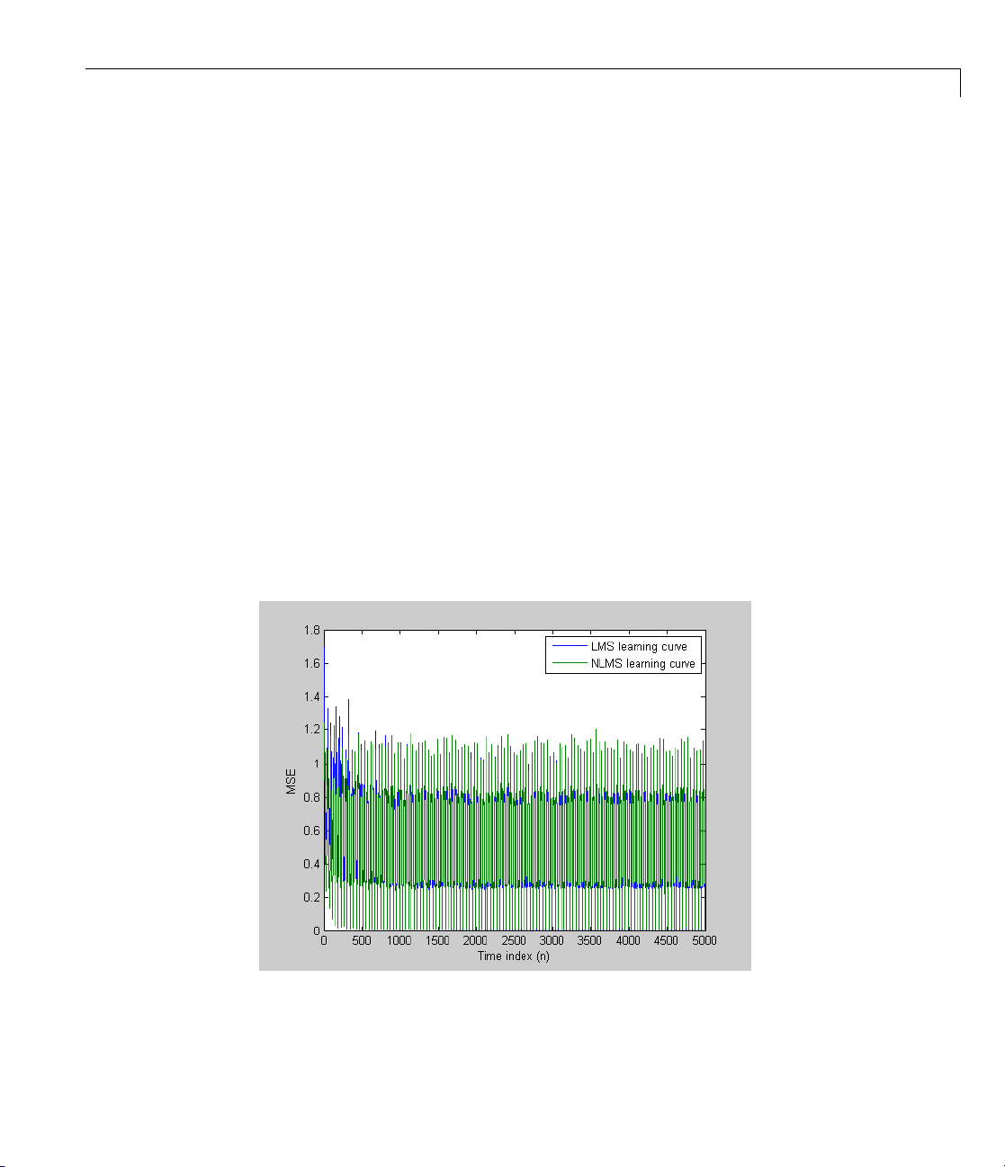
Compute the Lear
Now compute the m
every 10 samples
First, reset th
computed and t
reset(hlms);
reset(hnlms);
M = 10; % Decimation factor
mselms = msesim(hlms,v2,x,M);
msenlms = msesim(hnlms,v2,x,M);
plot(1:M:n(end),[mselms,msenlms])
legend('LMS learning curve','NLMS learning curve')
xlabel('Time index (n)');
ylabel('MSE');
In the nex
t plot you see the calculated learning curves for the LMS and
NLMS adap
.
e a daptive filters to avoid using the coefficients it has already
he states it has stored.
tive filters.
ning Curves
ean-square error. To speed things up, compute the error
5-9

5 Designing Adaptive Filters
Compute the Theo
For the LMS and NL
the theoretical
(MMSE) the exce
coefficients.
MATLAB may tak
thecodeplots
reset(hlms);
[mmselms,emselms,meanwlms,pmselms] = msepred(hlms,v2,x,M);
plot(1:M:n(end),[mmselms*ones(500,1),emselms*ones(500,1),...
legend('MMSE','EMSE','predicted LMS learning curve',...
'LMS learning curve')
xlabel('Time index (n)');
ylabel('MSE');
learning curves , along with the minimum mean-square error
ss mean-square error (EMSE) and the mean value of the
esometimetocalculatethecurves. Thefigureshownafter
the p redicted and actual LMS curves.
pmselms,mselms])
retical Learning Curves
MS algorithms, functions in the toolbox help you compute
5-10

Examples
Use this list to find examples in the documentation.
A

A Examples
Getting Started
Example — Design
“Floating-Point to Fixed-Point Conversion” on page 4-3
“Adaptive Filters Tutorial” on page 5-2
Using Filterbuilder
Example — Usi
aFilterinTwoStepsonpage2-4
ng Filterbuilder to Design a Simple Filter on page 2-9
A-2

Index
IndexD
data types 4-11
fixed 4-11
fixed-point
floating-point 4-11
single 4-11
decimation factor 3-2
decimator 3-2
design a filter 2-4
filterbuilder 2-9
F
filter cost 3-2
filter design
adaptive filter 5-2
Filter Design
Multirate 3-8
Multistage 3-8
Narrow Transition-Band 3-8
filterbuilder 2-9
fixed-point filter 4-2
conversion from floating-point 4-3
definition 4-2
G
getting started 2-2
getting started example 2-2
I
interpolator 3-2
M
Mfactor 3-2
multirate filter
definition 3-2
multistage filter
definition 3-6
uses 3-6
T
toolbox
getting started 2-2
Index-1
 Loading...