

Page 1

Filter Design Tool
Reference Guide
box™ 4
Page 2

How to Contact The MathWorks
www.mathworks.
comp.soft-sys.matlab Newsgroup
www.mathworks.com/contact_TS.html T echnical Support
suggest@mathworks.com Product enhancement suggestions
bugs@mathwo
doc@mathworks.com Documentation error reports
service@mathworks.com Order status, license renewals, passcodes
info@mathwo
com
rks.com
rks.com
Web
Bug reports
Sales, prici
ng, and general information
508-647-7000 (Phone)
508-647-7001 (Fax)
The MathWorks, Inc.
3 Apple Hill Drive
Natick, MA 01760-2098
For contact information about worldwide offices, see the MathWorks Web site.
Filter Design Toolbox™ Reference Guide
© COPYRIGHT 2000–2010 by The MathWorks™, Inc.
The software described in this document is furnished under a license agreement. The software may be used
or copied only under the terms of the license agreement. No part of this manual may be photocopied or
reproduced in any form without prior written consent from The MathW orks, Inc.
FEDERAL ACQUISITION: This provision applies to all acquisitions of the Program and Documentation
by, for, or through the federal government of the United States. By accepting delivery of the Program
or Documentation, the government hereby agrees that this software or documen tation qualifies as
commercial computer software or commercial computer software documentation as such terms are used
or defined in FAR 12.212, DFARS Part 227.72, and DFARS 252.227-7014. Accordingly, the terms and
conditions of this Agreement and only those rights specified in this Agreement, shall pertain to and govern
theuse,modification,reproduction,release,performance,display,anddisclosureoftheProgramand
Documentation by the federal government (or other entity acquiring for or through the federal government)
and shall supersede any conflicting contractual terms or conditions. If this License fails to meet the
government’s needs or is inconsistent in any respect with federal procurement law, the government agrees
to return the Program and Docu mentation, unused, to The Mat hWorks, Inc.
Trademarks
MATLAB and Simulink are registered trademarks of The MathWorks, Inc. See
www.mathworks.com/trademarks for a list of additional trademarks. Other product or brand
names may be trademarks or registered trademarks of their respective holders.
Patents
The MathWorks products are protected by one or more U.S. patents. Please see
www.mathworks.com/patents for more information.
Page 3

Revision History
March 2007 Online only New for Version 4.1 (Release 2007a)
September 2007 Online only New for Version 4.2 (Release 2007b)
March 2008 Online only New for Version 4.3 (Release 2008a)
October 2008 Online only New for V ersion 4.4 (Release 2008b)
March 2009 Online only New for Version 4.5 (Release 2009a)
September 2009 Online only New for Version 4.6 (Release 2009b)
March 2010 Online only New for Version 4.7 (Release 2010a)
Page 4

Page 5

Function Reference
1
Adaptive Filters ................................... 1-2
Least Mean Squares
Recursive Least Squares
Affine Projection
Frequency D omain
Lattice
.......................................... 1-4
............................... 1-2
............................ 1-3
.................................. 1-3
................................ 1-4
Contents
Discrete-Time Filters
Filter Specifications — Response Types
Filter Specifications — Design Methods
Multirate Filters
GUIs
Filter Analysis
Fixed-Point Filters
Quantized F ilter Analysis
SOS Conversion
Filter Design
.............................................. 1-11
..................................... 1-12
...................................... 1-18
.............................. 1-5
................................... 1-10
................................. 1-15
.......................... 1-16
................................... 1-17
............. 1-7
............. 1-9
Filter Conversion
.................................. 1-19
v
Page 6

Functions — Alphabetical List
2
Reference for the Properties of Filter Objects
3
Fixed-Point Filter Properties ....................... 3-2
Overview o f Fixed-Point Filters
Fixed-Point Objects and Filters
Summary — Fixed-Point Filter Properties
Property De tails for Fixed-Point Filters
...................... 3-2
...................... 3-2
............. 3-5
............... 3-18
Adaptive Filter Properties
Property Sum m aries
Property De tails for Adaptive Filter Properties
References
Multirate Filter Properties
Property Sum m aries
Property De tails for Multirate Filter Properties
References
........................................ 3-115
........................................ 3-132
.......................... 3-102
............................... 3-102
......................... 3-116
............................... 3-116
......... 3-107
......... 3-121
Index
vi Contents
Page 7

Function Reference
Adaptive Filters (p. 1-2) Design adaptive filters
1
Discrete-Time F ilters (p. 1-5)
Filter Specifications — Response
Types (p. 1-7)
Filter Specifications — Design
Methods (p. 1-9)
Multirate Filters (p. 1-10) Design multirate filter objects
GUIs (p. 1-11) Use graphical user interface tools to
Filter Analysis (p. 1-12) Analyze filters and filter objects
Fixed-Point Filters (p. 1-15) Create fixed-point filters
Quantized Filter Analysis (p. 1-16) Analyze fixed-point filters
SOS Conversion (p. 1-17)
Filter Design (p. 1-18) Design filters (not object-based)
Filter Conversion (p. 1-19) Transform filters to other forms,
Design FIR and IIR discrete-time
filter objects
Create objects that specify filter
responses
Design filter objects from
specification objects
design filters
Work with second-order section
filters
or use features in filter to develop
another filter
Page 8

1 Function Reference
Adaptive Filters
Least Mean Squares (p. 1-2) Filter w ith LMS techniques
Recursive L east Squares (p. 1-3) Filter with RLS techniques
Affine Projection (p. 1-3) Filter with affine projection
Frequency Domain (p. 1-4) Filter in the frequency domain
Lattice (p. 1-4) Filter with lattice filters
Least Mean Squares
adaptfilt.adjlms
adaptfilt.blms
adaptfilt.blmsfft
adaptfilt.dlms
adaptfilt.filtxlms
adaptfilt.lms
adaptfilt.nlms
adaptfilt.sd
adaptfilt.se
adaptfilt.ss
FIR a da ptive filter that uses adjoint
LMS algorithm
FIR adaptive filter that uses BLM S
FIR adaptive filter that uses
FFT-based BLMS
FIR adaptive filter that uses delayed
LMS
FIR adaptive filter that uses
filtered-x LMS
FIR adaptive filter that uses LMS
FIR adaptive filter that uses NLMS
FIR adaptive filter that uses
sign-data algorithm
FIR adaptive filter that uses
sign-error algorithm
FIR adaptive filter that uses
sign-sign algorithm
1-2
Page 9

Recursive Least Squares
Adaptive Filters
adaptfilt.ftf
adaptfilt.hrls
adaptfilt.hswrls
adaptfilt.qrdrls
adaptfilt.rls
adaptfilt.swftf
adaptfilt.swrls
Affine Projection
adaptfilt.ap
adaptfilt.apru
adaptfilt.bap
Fast transversal LMS adaptive filter
FIR adaptive filter that uses
householder (RLS)
FIR adaptive filter that uses
householder sliding window RLS
FIR adaptive filter that uses
QR-decomposition-based RLS
FIR adaptive filter that uses direct
form RLS
FIR adaptive filter that uses sliding
window fast transversal least
squares
FIR adaptive filter that uses window
recursive least squares (RLS)
FIR adaptive filter that uses direct
matrix inversion
FIR adaptive filter that uses
recursive matrix updating
FIR adaptive filter that uses block
affine projection
1-3
Page 10

1 Function Reference
Frequency Domain
adaptfilt.fdaf
adaptfilt.pbfdaf
adaptfilt.pbufdaf
adaptfilt.tdafdct
adaptfilt.tdafdft
adaptfilt.ufdaf
Lattice
adaptfilt.gal
adaptfilt.lsl
adaptfilt.qrdlsl
FIR adaptive filter that uses
frequency-domain with bin step size
normalization
FIR adaptive filter that uses
PBFDAF with bin step size
normalization
FIR adaptive filter that uses
PBUFDAF with bin ste p size
normalization
Adaptive filter that uses discrete
cosine transform
Adaptive filter that uses discrete
Fourier transform
FIR adaptive filter that uses
unconstrained frequency-domain
with quantized step size
normalization
FIR adaptive filter that uses
gradient lattice
Adaptive filter that uses LSL
Adaptive filter that uses
QR-decomposition-based LSL
1-4
Page 11

Discrete-Time Filters
Discrete-Time Filters
dfilt
dfilt.allpass
dfilt.calattice
dfilt.calatticepc
dfilt.cascade
dfilt.cascadeallpass
dfilt.cascadewdfallpass
dfilt.delay
dfilt.df1
dfilt.df1sos
dfilt.df1t
dfilt.df1tsos
dfilt.df2
dfilt.df2sos
dfilt.df2t
dfilt.df2tsos
dfilt.dfasymfir
dfilt.dffir
Discrete-time filter
Allpass filter
Coupled-allpass, lattice filter
Coupled-allpass,
power-complementary lattice filter
Cascade of discrete-time filters
Cascade of allpass discrete-time
filters
Cascade allpass WDF filters to
construct allpass WDF
Delay filter
Discrete-time, direct-form I filter
Discrete-time, SOS direct-form I
filter
Discrete-time, direct-form I
transposed filter
Discrete-time, SOS direct-form I
transposed filter
Discrete-time, direct-form II filter
Discrete-time, SOS, direct-form II
filter
Discrete-time, direct-form II
transposed filter
Discrete-time, SOS direct-form II
transposed filter
Discrete-time, direct-form
antisymmetric FIR filter
Discrete-time, direct-form FIR filter
1-5
Page 12

1 Function Reference
dfilt.dffirt
dfilt.dfsymfir
dfilt.farrowfd
dfilt.farrowlinearfd
dfilt.fftfir
dfilt.latticeallpass
dfilt.latticear
dfilt.latticearma
dfilt.latticemamax
dfilt.latticemamin
dfilt.parallel
dfilt.scalar
dfilt.wdfallpass
Discrete-time, direct-form FIR
transposed filter
Discrete-time, direct-form symmetric
FIR filter
Fractional Delay Farrow filter
Farrow Linear Fractional Delay
filter
Discrete-time, overlap-add, FIR
filter
Discrete-time, lattice allpass filter
Discrete-time, lattice, autoregressive
filter
Discrete-time, lattice,
autoregressive, moving-average
filter
Discrete-time, lattice,
moving-average filter with maximum
phase
Discrete-time, lattice,
moving-average filter with minimum
phase
Discrete-time, parallel structure
filter
Discrete-time, scalar filter
Wave digital allpass filter
1-6
Page 13

Filter Specifications — Response Types
Filter Specifications — Response Types
fdesign
fdesign.arbmag
fdesign.arbmagnphase
fdesign.audioweighting
fdesign.bandpass
fdesign.bandstop
fdesign.ciccomp
fdesign.comb
fdesign.decimator
fdesign.differentiator
fdesign.fracdelay
fdesign.halfband
fdesign.highpass
fdesign.hilbert
fdesign.interpolator
fdesign.isinclp
fdesign.lowpass
fdesign.notch
fdesign.nyquist
fdesign.octave
fdesign.parameq
Filter specification object
Arbitrary response magnitude filter
specification object
Arbitrary response magnitude and
phase filter specification object
Audio weighting filter specification
object
Bandpass filter specification object
Bandstop filter specification object
CIC compensator filter specification
object
IIR comb filter specification object
Decimator filter specification object
Differentiator filter specification
object
Fractional delay filter specification
object
Halfband filter specification object
Highpass filter specification object
Hilbert filter specification object
Interpolator filter specificatio n
Inverse-sinc filter specification
Lowpass filter specification
Notch filter specification
Nyquist filter specification
Octave filter specification
Parametric equalizer filter
specification
1-7
Page 14

1 Function Reference
fdesign.peak
fdesign.polysrc
fdesign.pulseshaping
fdesign.rsrc
Peak filter specification
Construct polynomial sample-rate
converter (POLYSRC) filter designer
Pulse-shaping filter specification
object
Rational-factor sample-rate
converter specification
1-8
Page 15

Filter Specifications — Design Methods
Filter Specifications — Design Methods
butter
cheby1
cheby2
designmethods
ellip
equiripple
fircls
ifir
iirlinphase
kaiserwin
maxflat
multistage
window
Butterworth IIR filter design using
specification object
Chebyshev Type I filter using
specification object
Chebyshev Type I I filter using
specification object
Methods available for designing
filter from specification object
Elliptic filter using specification
object
Equiripple single-rate or multirate
FIR filter from specification object
FIR Constrained Least Squares filter
Interpolated FIR filter from filter
specification
Quasi-linear phase IIR filter from
halfband filter specification
Kaiser window filter from
specification object
Maxflat FIR filter
Multistage filter from specification
object
FIR filter using windowed impulse
response
1-9
Page 16

1 Function Reference
Multirate Filters
mfilt.cascade
mfilt.cicdecim
mfilt.cicinterp
mfilt.farrowsrc
mfilt.fftfirinterp
mfilt.firdecim
mfilt.firfracdecim
mfilt.firfracinterp
mfilt.firinterp
mfilt.firsrc
mfilt.firtdecim
mfilt.holdinterp
mfilt.iirdecim
ilt.iirinterp
mf
mfilt.iirwdfdecim
mfilt.iirwdfinterp
mfilt.linearinterp
Cascade filter objects
Fixed-point CIC decimator
Fixed-point CIC interpolator
Sample rate converter with arbitrary
conversion factor
Overlap-add FIR polyphase
interpolator
Direct-form FIR polyphase decimator
Direct-form FIR polyphase fractional
decimator
Direct-form FIR polyphase fractional
interpolator
FIR filter-based interpolator
Direct-form FIR polyphase sample
rate converter
Direct-form transposed FIR filter
FIR hold interpolator
decimator
IIR
IIR interpolator
IIR wave digital filter decimator
IIR wave digital f il t er interpolator
Linear interpolator
1-10
Page 17

GUIs
GUIs
fdatool
filterbuilder
Open Filter Design and Analysis
Tool
GUI-based filter design
1-11
Page 18

1 Function Reference
Filter Analysis
autoscale
block
coeffs
cost
cumsec
denormalize
designmethods
designopts
disp
e
doubl
idfactors
eucl
coeffs
fft
ter
fil
ltstates.cic
fi
rtype
fi
reqrespest
f
freqrespopts
freqsamp
freqz
grpdelay
Automatic dynamic range scaling
Generate block from multirate filter
Coefficients for filters
Cost of using discrete-time or
multirate filter
Vector of SOS filters for cumulative
sections
Undo filter coefficient and gain
changes caused by
normalize
Methods available for designing
filter from specification object
Valid input arguments and values
for specification object and method
properties and values
Filter
ixed-point filter to use
Cast f
e-precision arithmetic
doubl
id factors for multirate filter
Eucl
uency-domain coefficients
Freq
terdatawithfilterobject
Fil
ore CIC filter states
St
pe of linear phase FIR filter
Ty
stimate fixed-point filter frequency
E
esponse through filtering
r
freqrespest
parameters and values
Real or complex frequency-sampled
FIR filter from specification object
Frequency response of filter
Filter group delay
1-12
Page 19

Filter Analysis
help
impz
isfir
islinphase
ismaxphase
isminphase
isreal
isstable
limitcycle
maxstep
measure
msepred
msesim
noisepsd
noisepsdopts
norm
normalize
normalizefreq
Help for design method with filter
specification
Filter impulse response
Determine whether filter is FIR
Determine whether filter is linear
phase
Determine whether filter is
maximum phase
Determine whether filter is
minimum phase
Determine whether filter uses real
coefficients
Determine whether filter is stable
Response of single-rate, fixed-point
IIR filter
Maximum step size for adaptive
filter convergence
Measure filter magnitude response
Predicted mean-squared error for
adaptive filter
Measured mean-squared error for
adaptive filter
Power spectral density of filter
output
Options for running filter output
noise PSD
P-norm of filter
Normalize filter numerator or
feed-forward coefficients
Switch filter specification between
normalized frequency and absolute
frequency
1-13
Page 20

1 Function Reference
nstates
order
phasedelay
phasez
polyphase
qreport
realizemdl
reffilter
reorder
reset
scale
scalecheck
set2int
setspecs
specifyall
stepz
validstructures
zerophase
zplane
Number of filter states
Order of fixed-point filter
Phase delay of filter
Unwrapped phase response for filter
Polyphase decomposition of
multirate filter
Most recent fixed-point filtering
operation report
Simulink®subsystem block for filter
Reference filter for fixed-point or
single-precision filter
Rearrange sections in SOS filter
Reset filter properties to initial
conditions
Scale sections of SOS filter
Check scaling of SOS filter
Configure filter for integer filtering
Specifications for filter specification
object
Fixed-point scaling modes in
direct-form FIR filter
Step response for filter
Structures for specification object
with design method
Zero-phase response for filter
Zero-pole plot for filter
1-14
To see the full listing of analysis m eth o d s that apply to the
or
mfilt objects, enter help adaptfilt, help dfilt,orhelp mfilt at the
MATLAB
®
prompt.
adaptfilt, dfilt,
Page 21

Fixed-Point Filters
Fixed-Point Filters
cell2sos
get
isreal
reset
scale
scalecheck
scaleopts
set
sos
sos2cell
Convert cell array to SOS matrix
Properties of quantized filter
Test if filter coefficients are real
Reset properties of quantized filter
to initial values
Scale sections of SOS filters
Check scaling of SOS filter
Scaling options for second-order
section scaling
Properties of quantized filter
Convert quantized filter to SOS
form, order, and scale
Convert SOS matrix to cell array
1-15
Page 22

1 Function Reference
Quantized Filter Analysis
freqz
impz
isallpass
isfir
islinphase
ismaxphase
isminphase
isreal
issos
isstable
noisepsd
noisepsdopts
zplane
Frequency response of filter
Filter impulse response
Determine whether filter is allpass
Determine whether filter is FIR
Determine whether filter is linear
phase
Determine whether filter is
maximum phase
Determine whether filter is
minimum phase
Determine whether filter uses real
coefficients
Determine whether filter is SOS
form
Determine whether filter is stable
Power spectral density of filter
output
Options for running filter output
noise PSD
Zero-pole plot for filter
1-16
Page 23

SOS Conversion
SOS Conversion
cell2sos
sos
sos2cell
Convert a cell array to a second-order
sections matrix
Convert a quantized filter to
second-order sections form, order,
and scale
Convert a second-order sections
matrix to a cell array
1-17
Page 24

1 Function Reference
Filter Design
farrow
fdatool
filterbuilder
fircband
firceqrip
fireqint
firgr
firhalfband
firlpnorm
firls
firminphase
firnyquist
ifir
iircomb
iirgrpdelay
iirlpnorm
iirlpnormc
iirnotch
iirpeak
Farrow filter
Open Filter Design and Analysis
Tool
GUI-based filter design
Constrained-band equiripple FIR
filter
Constrained, equiripple FIR filter
Equiripple FIR interpolators
Parks-McClellan FIR filter
Halfband FIR filter
Least P-norm optimal FIR filter
Least square linear-phase FIR filter
design
Minimum-phase FIR spectral factor
Lowpass Nyquist (Lth-band) FIR
filter
Interpolated FIR filter from filter
specification
IIR comb notch or peak filter
Optimal IIR filter with prescribed
group-delay
Least P-norm optimal IIR filter
Constrained least Pth-norm optimal
IIR filter
Second-order IIR notch filter
Second-order IIR peak or resonator
filter
1-18
Page 25

Filter Conversion
Filter Conversion
ca2tf
cl2tf
convert
firlp2hp
firlp2lp
iirlp2bp
iirlp2bs
iirlp2hp
iirlp2lp
iirpowcomp
set2int
tf2ca
tf2cl
Convert coupled allpass filter to
transfer function form
Convert coupled allpass lattice to
transfer function form
Convert filter structure of
discrete-time or multirate filter
Convert FIR lowpass filter to Type I
FIR highpass filter
Convert FIR Type I lowpass to
FIR Type 1 lowpass with inverse
bandwidth
Transform IIR lowpass filter to IIR
bandpass filter
Transform IIR lowpass filter to IIR
bandstop filter
Transform lowpass IIR filter to
highpass filter
Transform lowpass IIR filter to
different lowpass filter
Power complementary IIR filter
Configure filter for integer filtering
Transfer function to coupled allpass
Transfer function to coupled allpass
lattice
1-19
Page 26

1 Function Reference
1-20
Page 27

Functions — Alphabetical
List
2
Page 28

adaptfilt
Purpose Adaptive filter
Syntax ha = adaptfilt.algorithm('input1',input2,...)
Description ha = adaptfilt.algorithm('input1',input2,...) returns the
adaptive filter object
specified by
include an
Note that you do n ot enclose the algorithm option in single quotation
marks as you do for m ost strings. To construct an adaptive filter object
you must supply an
although every constructor creates a default adaptive filter when you do
not provide input arguments such as
syntax.
algorithm. When you construct an a daptive filter object,
algorithm specifier to implement a specific adaptive filter.
Algorithms
For adaptive filter (adaptfilt)objects,thealgorithm string
determines which adaptive filter algorithm your
implements. Each available algorithm entry appears in one of the tables
along with a brief d es cription of the algorithm. Click on the algorithm in
the first column to get more information about the associated adaptive
filter technique.
ha that uses the adaptive filtering technique
algorithm string — there is no default a lgorithm,
input1 or input2 in the calling
adaptfilt object
2-2
• “Least Mean Squares (LMS) Based FIR Adaptive Filters” on page 2-3
• “Recursive Least Squares (RLS) Based FIR Adaptive Filters” on
page 2-4
• “Affine Projection (AP) FIR Adaptive Filters” on page 2-4
• “FIR Adaptive Filters in the Frequency Domain (FD)” on page 2-5
• “Lattice Based (L) FIR Adaptive Filters” on page 2-5
Page 29

Least Mean Squares (LMS) Based FIR Adaptive Filters
adaptfilt
adaptfilt.algorithm
String
adaptfilt.adjlms
adaptfilt.blms
adaptfilt.blmsfft
adaptfilt.dlms
adaptfilt.filtxlms
adaptfilt.lms
adaptfilt.nlms
adaptfilt.sd
adaptfilt.se
adaptfilt.ss
Algorithm Used to Generate Filter
Coefficients
Use the Adjoint LM S FIR adaptive filter
algorithm
UsetheBlockLMSFIRadaptivefilter
algorithm
Use the FFT-based Block LMS FIR
adaptive filter algorithm
Use the delayed LMS FIR adaptive filter
algorithm
Use the filtered-x LMS FIR adaptive
filter algorithm
Use the LMS FIR adaptive filter
algorithm
Use the normalized LMS FIR adaptive
filter algorithm
Use the sign-data LMS FIR adaptive
filter algorithm
Use the sign-error LMS FIR adaptive
filter algorithm
Usethesign-signLMSFIRadaptivefilter
algorithm
For further information about an adapting algorithm, refer to the
reference page for the algorithm.
2-3
Page 30

adaptfilt
Recursive Least Squares ( RLS) Based FIR Adaptive Filters
adaptfilt.algorithm
String
adaptfilt.ftf
adaptfilt.qrdrls
adaptfilt.hrls
adaptfilt.hswrls
adaptfilt.rls
adaptfilt.swrls
adaptfilt.swftf
For more complete information about an adapting algorithm, refer to
the reference page for the algorithm.
Algorithm Used to Generate Filter
Coefficients
Use the fast transversal least squares
adaptation algorithm
Use the QR-decomposition RLS adaptation
algorithm
Use the householder RLS adaptation
algorithm
Use the householder SWRLS adaptation
algorithm
Use the recursive-least squares (RLS)
adaptation algorithm
Use the sliding window (SW) R LS adaptation
algorithm
Use the sliding window F TF adaptation
algorithm
Affine Projection (AP) FIR Adaptive Filters
2-4
adaptfilt.algorithm
String
adaptfilt.ap
adaptfilt.apru
adaptfilt.bap
Algorithm Used to Generate Filter
Coefficients
Use the affine projection algorithm that uses
direct matrix inversion
Use the affine projection algorithm that uses
recursive matrix updating
Usetheblockaffineprojectionadaptation
algorithm
Page 31

adaptfilt
To find more information about an adapting algorithm, refer to the
reference page for the algorithm.
FIR Adaptive Filters in the Frequency Domain ( FD)
adaptfilt.algorithm
String
adaptfilt.fdaf
adaptfilt.pbfdaf
adaptfilt.pbufdaf
adaptfilt.tdafdct
adaptfilt.tdafdft
adaptfilt.ufdaf
For more information about an adapting algorithm, refer to the
reference page for the algorithm.
Algorithm Used to Generate Filter
Coefficients
Use the frequency domain adaptation
algorithm
Use the partition block version of the FDAF
algorithm
Use the partition block unconstrained version
of the FDAF algorithm
Use the transform domain adaptation
algorithm using DCT
Use the transform domain adaptation
algorithm using DFT
Use the unconstrained FDAF algorithm for
adaptation
Lattice Based (L) FIR Adaptive Filters
adaptfilt.algorithm
String
adaptfilt.gal
adaptfilt.lsl
adaptfilt.qrdlsl
Algorithm Used to Generate Filter
Coefficients
Use the gradient adaptive lattice filter
adaptation algorithm
Use the least squares lattice adaptation
algorithm
Use the QR decomposition least squares lattice
adaptation algorithm
2-5
Page 32

adaptfilt
For more information about an adapting algorithm, refer to the
reference page for the algorithm.
Properties for All Adaptive Filter Objects
Each reference page for an algorithm and adaptfilt.algorithm object
specifies w hich properties apply to the adapting algorithm and how
to use them.
Methods for Adaptive Filter Objects
As is true with all objects, methods enable you to perform various
operations on
to the object handle that you assigned when you constructed the
adaptfilt object.
adaptfilt objects. To use the methods, you apply them
Most of the analysis methods that apply to
adaptfilt objects. Methods like freqz rely on the filter coefficients in
the
adaptfilt object. Since the coefficients change each time the filter
adapts to data, you should view the results of using a method as an
analysis of the filter a t a moment in time for the object. Use caution
when you apply an analysis method to your adaptive filter objects —
always check that your result approached your expectation.
In particular, the Filter Visualization Tool (FVTool) supports all of the
adaptfilt objects. Analyzing and viewing your adaptfilt objects is
straightforward — use the
fvtool(objectname)
to launch FVTool and work with your object.
Some methods share their names with functions in Signal Processing
Toolbox™ software, or even functions in this toolbox. Functions that
share names with methods behave in a similar way. Using the same
name for more than one function or method is called overloading and is
commoninmanytoolboxes.
fvtool method with the name of your object
dfilt objects also work with
2-6
Page 33

Method Description
adaptfilt/coefficients
Return the instantaneous adaptive
filter coefficients
adaptfilt/filter
Apply an adaptfilt object to your
signal
adaptfilt/freqz
Plot the instantaneous adaptive filter
frequency response
adaptfilt/grpdelay
Plot the instantaneous adaptive filter
group delay
adaptfilt/impz
Plot the instantaneous adaptive filter
impulse response.
adaptfilt/info
adaptfilt/isfir
Return the adaptive filter information.
Test whether an adaptive filter is an
finite impulse response (FIR) filters.
adaptfilt/islinphase
Testwhetheranadaptivefilterislinear
phase
adaptfilt/ismaxphase
Test whether an adaptive filter is
maximum phase
adaptfilt/isminphase
Test whether an adaptive filter is
minimum phase
adaptfilt/isreal
True whether an adaptive filter has real
coefficients
adaptfilt/isstable
adaptfilt/maxstep
Test whether an adaptive filter is stable
Return the maximum step size for an
adaptive filter
adaptfilt/msepred
adaptfilt/msesim
Return the predicted mean square error
Return the measured mean square error
via simulation.
adaptfilt
2-7
Page 34

adaptfilt
Method Description
adaptfilt/phasez
Plot the instantaneous adaptive filter
phase response
adaptfilt/reset
Reset an adaptive filter to initial
conditions
adaptfilt/stepz
Plot the instantaneous adaptive filter
step response
adaptfilt/tf
Return the instantaneous adaptive
filter transfer function
adaptfilt/zerophase
Plot the instantaneous adaptive filter
zerophase response
adaptfilt/zpk
Return a matrix containing the
instantaneous adaptive filter zero, p o le,
and gain values
adaptfilt/zplane
Plot the instantaneous adaptive filter
in the Z-plane
2-8
Working with Adaptive Filter Objects
The next sections cover viewing and changing the properties of
adaptfilt objects. Generally, modifying the properties is the same for
adaptfilt, dfilt,andmfilt obje cts and most of the same me thods
apply to all.
Viewing Object Properties
As with any object, you can use get to view a adaptfilt object’s
properties. To see a specific property, use
get(ha,'property')
To see all properties for an object, use
get(ha)
Page 35

adaptfilt
Changing Object Properties
To set specific properties, use
set(ha,'property1',value1,'property2',value2,...)
You must use single quotation marks around the property name so
MATLABtreatsthemasstrings.
Copying an Object
To create a copy of an object, use copy.
ha2 = copy(ha)
Note Using the syntax ha2 = ha copies only the object handle a nd does
not create a new object —
change the characteristics of
ha and ha2 are not independent. When you
ha2,thoseofha change as well.
Using Filter States
Two properties control your adaptive filter states.
•
States — stores the current states of the filter. Before the filter is
applied, the states correspond to the initial conditions and after the
filter is applied, the states correspond to the final conditions.
•
PersistentMemory — resets the filter before filtering. The default
value is
filter, such as
specified when you constructed the object, before you use the object
to filter data. Setting
to retain its current properties between filtering operations, rather
than resetting the filter to its property values at construction.
false which causes the properties that are modified by the
coefficients and states,toberesettothevalueyou
PersistentMemory to true allows the object
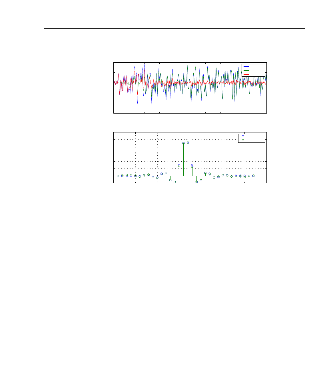
Examples Construct an LMS adaptive filter object and use it to identify an
unknown system. For this example, use 500 iteration of the adapting
process to determine the unknown filter coefficients. Using the LMS
2-9
Page 36

adaptfilt
algorithm represents one of the most straightforward technique for
adaptive filters.
x = randn(1,500); % Input to the filter
b = fir1(31,0.5); % FIR system to be identified
n = 0.1*randn(1,500); % Observation noise signal
d = filter(b,1,x)+n; % Desired signal
mu = 0.008; % LMS step size.
ha = adaptfilt.lms(32,mu);
[y,e] = filter(ha,x,d);
subplot(2,1,1); plot(1:500,[d;y;e]);
title('System Identification of an FIR Filter');
legend('Desired','Output','Error');
xlabel('Time Index'); ylabel('Signal Value');
subplot(2,1,2); stem([b.',ha.coefficients.']);
legend('Actual','Estimated');
xlabel('Coefficient #'); ylabel('Coefficient Value'); grid on;
Glancing at the figure shows you the coefficients after adapting closely
match the desired unknown FIR filter.
2-10
Page 37
adaptfilt
2
1
0
−1
Signal Value
−2
−3
0 50 100 150 200 250 300 350 400 450 500
0.6
0.5
0.4
0.3
0.2
0.1
Coefficient Value
0
−0.1
0 5 10 15 20 25 30 35
See Also dfilt, filter, mfilt
System Identification of an FIR Filter
Time Index
Coefficient #
Desired
Output
Error
Actual
Estimated
2-11
Page 38

adaptfilt.adjlms
Purpose FIR adaptive filter that uses adjoint LMS algorithm
Syntax ha = adaptfilt.adjlms(l,step,leakage,pathcoeffs,pathest,...
errstates,pstates,coeffs,states)
Description ha = adaptfilt.adjlms(l,step,leakage,pathcoeffs,pathest,...
errstates,pstates,coeffs,states)
adjoint LMS adaptive filter.
l is the adaptive filter length (the nu m ber
of coefficients or taps) and must be a positive integer.
10 when you omit the argument.
It must be a nonnegative scalar. When you omit the
step defaults to 0.1.
leakage is the adjoint LMS leakage factor. It must be a scalar between
0and1. When
of the
adjlms algorithm to determine the filter coefficients. leakage
leakage is less than one, you implement a leaky version
defaults to 1 specifying no leakage in the algorithm.
pathcoeffs is the secondary path filter model. This vector should
contain the coefficient values of the secondary path from the output
actuator to the error sensor.
constructs object ha, an FIR
l defaults to
step is the adjoint LMS step size.
step argument,
2-12
pathest istheestimateofthesecondarypathfiltermodel. pathest
defaults to the values in pathcoeffs.
errstates is a v ector of error states of the adaptive filter. It must have
a length equal to the filter order of the secondary path model estimate.
errstates defaults to a vector of zeros of appropriate length. pstates
contains the secondary path FIR filter states. It must be a vector of
length equal to the filter order of the secondary path model.
pstates
defaults to a vector of zeros of appropriate length. The initial filter
coefficients for the secondary path filter compose vector
be a length
states is a vector containing the initial filter states. It must be a vector
of length
states, it defaults to an appropriate length vector of zeros.
l vector. coeffs defaults to a length l vector of zeros.
l+ne-1, where ne is the length of errstates. When you omit
coeffs.Itmust
Page 39

adaptfilt.adjlms
Properties In the syntax for creating the adaptfilt object, the input options are
properties of the object created. This table lists the propertie s for the
adjoint LMS object, their default values, and a brief description of the
property.
Property Default Value Description
Algorithm
Coefficients
ErrorStates
FilterLength
Leakage 1
SecondaryPathCoeffs
SecondaryPathEstimate
None
Length l vector with
zeros for all elements
[0,...,0]
10
No default A vector that contains the coefficient
pathcoeffs
values
Specifies the adaptive filter algorithm
the object uses during adaptation
Adjoint LMS FIR filter coefficients.
Should be initialized with the
initial coefficients for the FIR filter
prior to adapting. You need
entries in coefficients.Updated
filter coefficients are returned in
coefficients when you use s as an
output argument.
Avectoroftheerrorstatesforyour
adaptive filter, with length equal to the
order of your secondary path filte r.
The number of coefficients in your
adaptive filter.
Specifies the leakage parameter.
Allows you to implement a leaky
algorithm. Including a leakage factor
can improve the results of the algorithm
by forcing the algorithm to continue to
adapt even after it reaches a minimum
value. Ranges between 0 and 1.
values of your secondary path from the
output actuator to the error sensor.
An estimate of the secondary path filter
model.
l
2-13
Page 40

adaptfilt.adjlms
Property Default Value Description
SecondaryPathStates
States
Stepsize
PersistentMemory false or true
Length of the
secondary path filter.
All elements are
zeros.
l+ne+1, where ne is
length(errstates)
0.1
The states of the secondary path filter,
the unknown system
Contains the initial conditions for your
adaptive filter and returns the states
of the FIR filter after adaptation. If
omitted, it defaults to a zero vector of
length equal to l+ne+1. When you use
adaptfilt.adjlms in a loop structure,
use this element to specify the initial
filter states for the adapting FIR filter.
Sets the adjoint LMS algorithm step
size used for each iteration of the
adapting algorithm. Determines
both how quickly and how closely the
adaptive filter converges to the filter
solution.
Determine whether the filter states
get restored to their starting values for
each filtering operation. The starting
values are the values in place when you
create the filter.
PersistentMemory
returnstozeroanystatethatthefilter
changes during processing. States
that the filter does not change are not
affected. Defaults to
false.
Example Demonstrate active noise control of a random noise signal that runs for
1000 samples.
x = randn(1,1000); % Noise source
g = fir1(47,0.4); % FIR primary path system model
2-14
Page 41

adaptfilt.adjlms
n = 0.1*randn(1,1000); % Observation noise signal
d = filter(g,1,x)+n; % Signal to be canceled (desired)
b = fir1(31,0.5); % FIR secondary path system model
mu = 0.008; % Adjoint LMS step size
ha = adaptfilt.adjlms(32,mu,1,b);
[y,e] = filter(ha,x,d);
plot(1:1000,d,'b',1:1000,e,'r');
title('Active Noise Control of a Random Noise Signal');
legend('Original','Attenuated');
xlabel('Time Index'); ylabel('Signal Value'); grid on;
Reviewing the figure shows that the adaptive filter attenuates the
original noise signal as you expect.
2
1.5
1
0.5
0
Signal Value
−0.5
−1
−1.5
−2
0 100 200 300 400 500 600 700 800 900 1000
Active Noise Control of a Random Noise Signal
Time Index
See Also adaptfilt.dlms, adaptfilt.filtxlms
Original
Attenuated
2-15
Page 42

adaptfilt.adjlms
References Wan, Eric., “Adjoint LMS: An Alternative to Filtered-X LMS and
Multiple Error LMS,” Proceedings of the International Conference on
Acoustics, Speech, and Signal Processing (ICASSP), pp. 1841-1845,
1997
2-16
Page 43

adaptfilt.ap
Purpose FIR adaptive filter that uses direct matrix inversion
Syntax ha = adaptfilt.ap(l,step,projectord,offset,coeffs,states,...
errstates,epsstates)
Description ha =
adaptfilt.ap(l,step,projectord,offset,coeffs,states,...
errstates,epsstates)
filter
ha using direct matrix inversion.
Input Arguments
Entries in the following table describe the input arguments for
adaptfilt.ap.
Input
Argument Description
l
step
projectord
offset
Adaptive filter length (the number of coefficients or
taps) and it must be a p ositiv e integer.
10.
Affine projection step size. Thisisascalarthat
should be a value between zero and one. Setting
equal to one provides the fastest convergence during
adaptation.
Projection order of the affine projection algorithm.
projectord defines the size of the input signal
covariance matrix and defaults to two.
Offset for the input signal covariance matrix. You
should initialize the covariance matrix to a diagonal
matrix w h ose diagonal entries are equal to the offset
you specify.
defaults to one.
constructs an affine projection FIR adaptive
l defaults to
step
step defaults to 1.
offset should be positive. offset
2-17
Page 44

adaptfilt.ap
Input
Argument Description
coeffs
states
errstates
epsstates
Properties Since your adaptfilt.ap filter is an object, it has properties that de fine
its behavior in operation. Note that many of the properties are also
input arguments for creating
properties that apply, this table lists and describes each property for
the affine projection filter object.
Vector containing the initial filter coefficients. It m ust
be a length
coeffs defaults to length l vector of zeros when you
l vector, the number of filter coefficients.
do not provide the argument for input.
Vector of the adaptive filter states. states defaults
to a vector of zeros which has length equal to (
projectord -2).
Vector of the adaptive filter error states. errstates
defaults to a zero vector with l ength equal to
(
projectord -1).
Vector of the epsilon values of the adaptive filter.
epsstates defaults to a vector of zeros with
(
projectord -1)elements.
adaptfilt.ap objects. To show you the
l +
2-18
Name Range Description
Algorithm
None
Defines the adaptive filter
algorithm the object uses during
adaptation
FilterLength
Any positive
integer
Reports the length of the filter,
the number of coefficients or taps
Page 45

Name Range Description
ProjectionOrder
1toaslarge
as needed.
Projection order of the
affine projection algorithm.
ProjectionOrder defines the
size of the input signal covariance
matrix and defaults to two.
OffsetCov
Coefficients
Matrix of
values
Vector of
elements
Contains the offset covariance
matrix
Vector containing the initial filter
coefficients. It must be a length
l vector, the number of filter
coefficients.
length
l vector of zeros when you
do not provide the argument for
input.
States
ErrorStates
Vector of
elements,
data type
double
Vector of
elements
Vector of the adaptive filter
states. states defaults to a vector
of zeros which has length equal
to (
l + projectord -2).
Vector of the adaptive filter error
states.
errstates defaults to a
zero vector with length equal to
(
projectord -1).
EpsilonStates
Vector of
elements
Vector of the epsilon values of
theadaptivefilter.
defaults to a vector of zeros with
(
projectord -1)elements.
adaptfilt.ap
coeffs defaults to
epsstates
2-19
Page 46

adaptfilt.ap
Name Range Description
StepSize
PersistentMemory false or true
Example Quadrature phase shift keying (QPSK) adaptive equalization using a
32-coefficient F IR filter. Run the adaptation for 1000 iterations.
Any scalar
from zero to
one, inclusive
Specifies the step size taken
between filter coefficient u pdate s
Determine whether the filter
states get restored to their
starting values for each
filtering operation. The starting
values are the values in place
when you create the filter.
PersistentMemory returns to
zero any state that the filter
changes during processing.
States that the filter does not
change are not affected. Defaults
to
true.
2-20
D = 16; % Number of samples of delay
b = exp(j*pi/4)*[-0.7 1]; % Numerator coefficients of channel
a = [1 -0.7]; % Denominator coefficients of channel
ntr= 1000; % Number of iterations
s = sign(randn(1,ntr+D)) + j*sign(randn(1,ntr+D));% Baseband Signal
n = 0.1*(randn(1,ntr+D) + j*randn(1,ntr+D)); % Noise signal
r = filter(b,a,s)+n; % Received signal
x = r(1+D:ntr+D); % Input signal (received signal)
d = s(1:ntr); % Desired signal (delayed QPSK signal)
mu = 0.1; % Step size
po = 4; % Projection order
offset = 0.05; % Offset for covariance matrix
ha = adaptfilt.ap(32,mu,po,offset);
[y,e] = filter(ha,x,d);
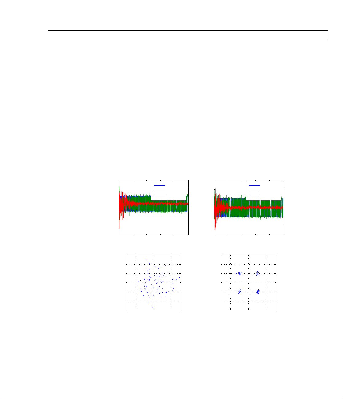
subplot(2,2,1); plot(1:ntr,real([d;y;e])); title('In-Phase Components');
Page 47

adaptfilt.ap
legend('Desired','Output','Error');
xlabel('Time Index'); ylabel('Signal Value');
subplot(2,2,2); plot(1:ntr,imag([d;y;e]));
title('Quadrature Components');
legend('Desired','Output','Error');
xlabel('Time Index'); ylabel('Signal Value');
subplot(2,2,3); plot(x(ntr-100:ntr),'.');
axis([-3 3 -3 3]); title('Received Signal Scatter Plot');
axis('square'); xlabel('Real[x]'); ylabel('Imag[x]'); grid on;
subplot(2,2,4); plot(y(ntr-100:ntr),'.'); axis([-3 3 -3 3]);
title('Equalized Signal Scatter Plot');
axis('square'); xlabel('Real[y]'); ylabel('Imag[y]'); grid on;
The four plots shown revea
2
1
0
Signal Value
−1
−2
0 200 400 600 800 1000
Imag[x]
−1
−2
−3
See Also msesim
In−Phase Components
Time Index
Received Signal Scatter Plot
3
2
1
0
−2 0 2
Real[x]
Desired
Output
Error
l the QPSK process at work.
Quadrature Components
3
2
1
0
Signal Value
−1
−2
−3
0 200 400 600 800 1000
3
2
1
0
Imag[y]
−1
−2
−3
Time Index
Equalized Signal Scatter Plot
−2 0 2
Real[y]
Desired
Output
Error
2-21
Page 48

adaptfilt.ap
References [1] Ozeki, K. and Umeda, T., “An Adaptive Filtering Algorithm Using
an Orthogonal Projection to an Affine Subspace and Its Properties,”
Electronics and Communications in Japan, vol.67-A, no. 5, pp. 19-27,
May 1984
[2] Maruyama, Y., “A Fast Method of Projection Algorithm,” Proc. 1990
IEICE Spring Conf., B-744
2-22
Page 49

adaptfilt.apru
Purpose FIR adaptive filter that uses recursive matrix updating
Syntax ha = adaptfilt.apru(l,step,projectord,offset,coeffs,states,
...errstates,epsstates)
Description ha = adaptfilt.apru(l,step,projectord,offset,coeffs,states,
...errstates,epsstates)
filter
ha using recursive matrix updating.
Input Arguments
Entries in the following table describe the input arguments for
adaptfilt.apru.
Input
Argument Description
l
step
projectord
offset
coeffs
Adaptive filter length (the number of coefficients or
taps). It must be a positive integer.
Affine projection step size. This is a scalar that
should be a value between zero and one. Setting
equal to one provides the fastest convergence during
adaptation.
Projection order of the affine projection algorithm.
projectord defines the size of the input signal
covariance matrix and defaults to two.
Offset for the input signal covariance matrix. You
should initialize the covariance matrix to a diagonal
matrix whose diagon al entries are equ a l to the offset
you specify.
defaults to one.
Vector containing the initial filter coefficients. It must
be a length
coeffs defaults to length l vector of zeros when you
do not provide the argument for input.
constructs an affine projection FIR adaptive
l defaults to 10.
step
step defaults to 1.
offset should be positive. offset
l vector, the number of filter coefficients.
2-23
Page 50

adaptfilt.apru
Input
Argument Description
states
errstates
epsstates
Properties Since your adaptfilt.apru filter is an object, it has properties that
define its behavior in operation. Note that many of the properties are
also input arguments for creating
the properties that apply, this table lists and describes each property
for the affine projection filter object.
Vector of the adaptive filter states. states defaults
to a vector of zeros which has length equal t o (
projectord -2).
Vector of the adaptive filter error states. errstates
defaults to a zero vector with length equal to
(
projectord -1).
Vector of the epsilon values of the a daptive filter.
epsstates defaults to a vector of zeros with
(
projectord -1)elements.
adaptfilt.apru objects. To show you
l +
2-24
Name Range Description
Algorithm
None
Defines the adaptive filter
algorithm the object uses
during adaptation
FilterLength
Any positive
integer
Reports the length of the filter,
the number of coefficients or
taps
ProjectionOrder
1toaslarge
as needed.
Projection order of the
affine projection algorithm.
ProjectionOrder defines
the size of the input signal
covariance matrix and defaults
to two.
Page 51

Name Range Description
OffsetCov
Coefficients
Matrix of
values
Vector of
elements
Contains the offset covariance
matrix
Vector containing the initial
filter coefficients. It must be
alength
l vector, the number
of filter coefficients.
defaults to length l vector of
zeros w hen you do not provide
the a rgument for input.
States
Vector of
elements,
data type
double
Vector of the adaptive filter
states. states defaults to
a vector of zeros which has
length equal to (
-2).
ErrorStates
Vector of
elements
Vector of the adaptive filter
error states.
defaults to a zero vector with
length equal to (
1).
EpsilonStates
Vector of
elements
Vector of the epsilon values of
the adaptive filter.
defaults to a vector of zeros
with (
projectord -1)elements.
adaptfilt.apru
coeffs
l + projectord
errstates
projectord -
epsstates
2-25
Page 52

adaptfilt.apru
Name Range Description
StepSize
PersistentMemory false or true
Example Demonstrate quadrature phase shift keying (QPSK) adaptive
equalization using a 32-coefficient FIR filter. This example runs the
adaptation process for 1000 iterations.
Any scalar
from zero to
one, inclusive
Specifies the step size taken
between filter coefficient
updates
Determine whether the filter
states get restored to their
starting values for each
filtering operation. The
starting values are the values
in place when you create the
filter.
PersistentMemory
returns to zero any state
that the filter changes during
processing. States that the
filter does not change are not
affected. Defaults to
true.
2-26
D = 16; % Number of samples of delay
b = exp(j*pi/4)*[-0.7 1]; % Numerator coefficients of channel
a = [1 -0.7]; % Denominator coefficients of channel
ntr= 1000; % Number of iterations
s = sign(randn(1,ntr+D)) + j*sign(randn(1,ntr+D)); % Baseband
n = 0.1*(randn(1,ntr+D) + j*randn(1,ntr+D)); % Noise signal
r = filter(b,a,s)+n; % Received signal
x = r(1+D:ntr+D); % Input signal (received signal)
d = s(1:ntr); % Desired signal (delayed QPSK signal)
mu = 0.1; % Step size
po = 4; % Projection order
del = 0.05; % Offset
ha = adaptfilt.apru(32,mu,po,offset); [y,e] = filter(ha,x,d);
subplot(2,2,1); plot(1:ntr,real([d;y;e])); title('In-Phase Components');
Page 53
adaptfilt.apru
legend('Desired','Output','Error');
xlabel('Time Index'); ylabel('Signal Value');
subplot(2,2,2); plot(1:ntr,imag([d;y;e])); title('Quadrature Components');
legend('Desired','Output','Error');
xlabel('Time Index'); ylabel('Signal Value');
subplot(2,2,3); plot(x(ntr-100:ntr),'.'); axis([-3 3 -3 3]);
title('Received Signal Scatter Plot');
axis('square'); xlabel('Real[x]'); ylabel('Imag[x]'); grid on;
subplot(2,2,4); plot(y(ntr-100:ntr),'.'); axis([-3 3 -3 3]);
title('Equalized Signal Scatter Plot');
axis('square'); xlabel('Real[y]'); ylabel('Imag[y]'); grid on;
In the following component and scatter plots, you see the results of
QPSK equalization.
3
2
1
0
−1
Signal Value
−2
−3
−4
In−Phase Components
Desired
Output
Error
0 200 400 600 800 1000
3
2
1
0
Imag[x]
−1
−2
−3
Time Index
Received Signal Scatter Plot
−2 0 2
Real[x]
Quadrature Components
3
2
1
0
Signal Value
−1
−2
−3
0 200 400 600 800 1000
3
2
1
0
Imag[y]
−1
−2
−3
Time Index
Equalized Signal Scatter Plot
−2 0 2
Real[y]
Desired
Output
Error
2-27
Page 54

adaptfilt.apru
See Also adaptfilt, adaptfilt.ap, adaptfilt.bap
References [1] Ozeki. K., T. Omeda, “An Adaptive Filtering Algorithm Using
an Orthogonal Projection to an Affine Subspace and Its Properties,”
Electronics and Communications in Japan, vol. 67-A, no. 5, pp. 19-27,
May 1984
[2] Maruyama, Y, “A Fast Method of Projection Algo rithm,” Proceedings
1990 IEICE Spring Conference, B-744
2-28
Page 55

adaptfilt.bap
Purpose FIR adaptive f ilter that uses block affine pr ojection
Syntax ha = adaptfilt.bap(l,step,projectord,offset,coeffs,states)
Description ha = adaptfilt.bap(l,step,projectord,offset,coeffs,states)
constructs a block affine projection FIR adaptive filter ha.
Input Arguments
Entries in the following table describe the input arguments for
adaptfilt.bap.
Input
Argument Description
l
step
projectord
offset
Adaptive filter length (the number of coefficients
or taps) and it must be a positive integer.
defaults to 10.
Affine projection step size. This is a scalar that
should be a value between zero and one. Setting
step equal to one provides the fastest convergence
during adaptation.
Projection order of the affine projection algorithm.
projectord defines the size of the input signal
covariance matrix and defaults to two.
Offset for the input signal covariance matrix.
You should initialize the covariance matrix to a
diagonal matrix whose diagonal entries are equal
to the offset y ou specify.
offset defaults to one.
step defaults to 1.
offset should be positive.
l
2-29
Page 56

adaptfilt.bap
Input
Argument Description
coeffs
states
Properties Since your adaptfilt.bap filter is an object, it has properties that
define its behavior in operation. Note that many of the properties are
also input arguments for creating
the properties that apply, this table lists and describes each property
for the affine projection filter object.
Name Range Description
Algorithm
FilterLength
ProjectionOrder
OffsetCov
Vector containing the initial filter coefficients. It
must be a length
coefficients.
zeros when you do not provide the argument for
input.
Vector of the adaptive filter states. states defaults
to a vector of zeros which has length equal to (
+ projectord -2).
None
Any positive
integer
1 to as large as
needed.
Matrix of values Contains the offset
l vector, the number of filter
coeffs defaults to length l vector of
adaptfilt.bap objects. To show you
Defines the adaptive filter
algorithm the object uses
during adaptation
Reports the length of
the filter, the number of
coefficients or taps
Projection order of the
affine projection algorithm.
ProjectionOrder defines
thesizeoftheinputsignal
covariance matrix and
defaults to two.
covariance matrix
l
2-30
Page 57

Name Range Description
Coefficients
Vector of
elements
Vector containing the initial
filter coefficients. It must
be a length
number of filter coefficients.
coeffs defaults to length l
vector of zeros when you do
not provide the argument for
input.
States
Vector of
elements, data
type double
Vector of the adaptive filter
states. states defaults to
a vector of zeros which
has length equal to (
projectord -2).
StepSize
PersistentMemory false or true
Any scalar from
zero to one,
inclusive
Specifies the step size taken
between filter coefficient
updates
Determine whether the filter
states get restored to their
starting values for each
filtering operation. The
starting values are the values
inplacewhenyoucreatethe
filter.
PersistentMemory
returns to zero any state
that the filter changes during
processing. States that the
filter does not change are not
affected. Defaults to
adaptfilt.bap
l vector, the
l +
true.
Example Show an example of quadrature phase shift keying (QPSK) adaptive
equalization using a 32-coefficient FIR filter.
D = 16; % delay
2-31
Page 58

adaptfilt.bap
b = exp(j*pi/4)*[-0.7 1]; % Numerator coefficients
a = [1 -0.7]; % Denominator coefficients
ntr= 1000; % Number of iterations
s = sign(randn(1,ntr+D))+j*sign(randn(1,ntr+D));% Baseband signal
n = 0.1*(randn(1,ntr+D) + j*randn(1,ntr+D)); % Noise signal
r = filter(b,a,s)+n; % Received signal
x = r(1+D:ntr+D); % Input signal (received signal)
d = s(1:ntr); % Desired signal (delayed QPSK signal)
mu = 0.5; % Step size
po = 4; % Projection order
offset = 1.0; % Offset for covariance matrix
ha = adaptfilt.bap(32,mu,po,offset);
[y,e] = filter(ha,x,d); subplot(2,2,1);
plot(1:ntr,real([d;y;e]));
title('In-Phase Components'); legend('Desired','Output','Error');
xlabel('Time Index'); ylabel('Signal Value');
subplot(2,2,2); plot(1:ntr,imag([d;y;e]));
title('Quadrature Components');
legend('Desired','Output','Error');
xlabel('Time Index'); ylabel('Signal Value');
subplot(2,2,3); plot(x(ntr-100:ntr),'.'); axis([-3 3 -3 3]);
title('Received Signal Scatter Plot'); axis('square');
xlabel('Real[x]'); ylabel('Imag[x]'); grid on;
subplot(2,2,4); plot(y(ntr-100:ntr),'.'); axis([-3 3 -3 3]);
title('Equalized Signal Scatter Plot'); axis('square');
xlabel('Real[y]'); ylabel('Imag[y]'); grid on;
2-32
Page 59

adaptfilt.bap
4
2
0
Signal Value
−2
−4
In−Phase Components
Desired
Output
Error
0 200 400 600 800 1000
3
2
1
0
Imag[x]
−1
−2
−3
Time Index
Received Signal Scatter Plot
−2 0 2
Real[x]
−1
Signal Value
−2
−3
−4
Quadrature Components
3
2
1
0
0 200 400 600 800 1000
3
2
1
0
Imag[y]
−1
−2
−3
Time Index
Equalized Signal Scatter Plot
−2 0 2
Real[y]
Desired
Output
Error
Using the block affine projection object in QPSK results in the plots
shown here.
See Also adaptfilt, adaptfilt.ap, adaptfilt.apru
References [1] Ozeki, K. and T. Omeda, “An Adaptive Filtering Algorithm Using
an Orthogonal Projection to an Affine Subspace and Its Properties,”
Electronics and Communications in Japan, vol. 67-A, no. 5, pp. 19-27,
May 1984
[2] Montazeri, M. and Duhamel, P, “A S et of Algorithms Linking NLMS
and Block RLS Algorithms,” IEEE Transactions Signal Processing, vol.
43, no. 2, pp, 444-453, February 1995
2-33
Page 60

adaptfilt.blms
Purpose FIR adaptive filter that uses BLMS
Syntax ha = adaptfilt.blms(l,step,leakage,blocklen,coeffs,states)
Description ha = adaptfilt.blms(l,step,leakage,blocklen,coeffs,states)
constructs an FIR block LMS adaptive filter ha,wherel is the adaptive
filter length (the number of coefficients or taps) and must be a positive
integer.
step is the block LMS step size. You must set step to a nonnegative
scalar. You can use function
of step size values for the signals being processed. When unspecified,
step defaults to 0.
leakage is the block LMS leakag e factor. It must be a scalar between 0
and 1 . If you se t leakage to be less than one, you implement the leaky
block LMS algorithm.
the adapting a lgorithm .
blocklen is the block length used. It must be a positive inte ger and
the signal vectors
block lengths result in faster per-sample execution times but with
poor adaptation characteristics. When you choose
blocklen + length(coeffs) is a power of 2, use adaptfilt.blmsfft.
blocklen defaults to l.
l defaults to 10.
maxstep to determine a reasonable range
leakage defaults to 1 specifying no leakage in
d and x should be divisible by blocklen.Larger
blocklen such that
coeffs is a vector of initial filter coefficients. it must be a length l
vector. coeffs defaults to length l vector of zeros.
states contains a vector of your initial filter states. It must be a length
l vector and defaults to a length l vector of zeros when you do not
include it in your calling function.
Properties In the syntax for creating the adaptfilt object, the input options are
properties of the object created. This table lists the propertie s for the
adjoint LMS object, their default values, and a brief description of the
property.
2-34
Page 61

Property
Algorithm
FilterLength
Coefficients
States
Leakage
BlockLength
Default
Value Description
None
Defines the adaptive filter algorithm
the object uses during adaptation
Any
positive
Reports the length of the filter, the
number o f coefficients or taps
integer
Vector of
elements
Vector containing the initial filter
coefficients. It must be a length
l vector where l is the number of
filter coefficients.
length
l vector of zeros when you do
not provide the argument for input.
Vector of
elements
Vector of the adaptive filter states.
states defaults to a vector of zeros
which has length equal to
Specifies the leakage parameter.
Allows you to implement a leaky
algorithm. Including a leakage
factor can improve the results of the
algorithm by forcing the algorithm
to continue to adapt even after it
reaches a minimum value. Ranges
between 0 and 1.
Vector of
length
Size of the blocks of data processed
in each iteration
l
adaptfilt.blms
coeffs defaults to
l
2-35
Page 62

adaptfilt.blms
Default
Property
StepSize
PersistentMemory false or
Value Description
0.1
true
Sets the block LMS algorithm step
size used for each iteration of the
adapting algorithm. Determines
both how quickly and how closely the
adaptive filter converges to the filter
solution. Use
maxstep to determine
the maximum usable step size.
Determine whether the filter states
get restored to their starting values
for each filtering operation. The
starting values are the values in
place when you create the filter.
PersistentMemory returns to zero
any state that the filter changes
during processing. States that
the filter does not change are not
affected. Defaults to
false.
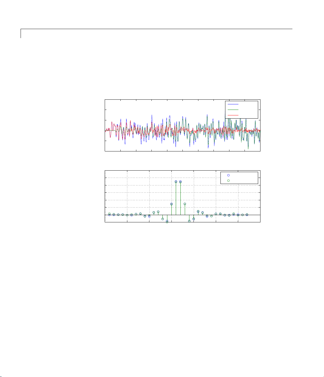
Example Use an adaptive filter to identify an unknown 32nd-order FIR filter.
In this example 500 input samples result in 500 iterations of the
adaptation process. You see in the plot that follows the example code
that the adaptive filter has determined the coefficients of the unknown
system under test.
x = randn(1,500); % Input to the filter
b = fir1(31,0.5); % FIR system to be identified
no = 0.1*randn(1,500); % Observation noise signal
d = filter(b,1,x)+no; % Desired signal
mu = 0.008; % Block LMS step size
n = 5; % Block length
ha = adaptfilt.blms(32,mu,1,n);
[y,e] = filter(ha,x,d);
subplot(2,1,1); plot(1:500,[d;y;e]);
2-36
Page 63

adaptfilt.blms
0
title('System Identification of an FIR Filter');
legend('Desired','Output','Error');
xlabel('Time Index'); ylabel('Signal Value');
subplot(2,1,2); stem([b.',ha.coefficients.']);
legend('Actual','Estimated');
xlabel('Coefficient #'); ylabel('Coefficient Value');
grid on;
Based on looking at the figures here, the adaptive filter correctly
identified the unknown system after 500 iterations, or few er. In the
lower plo t, you see the comparison between the actual filter coefficients
and those determined by the adaptation process.
3
2
1
0
Signal Value
−1
−2
−3
0 50 100 150 200 250 300 350 400 450 50
0.6
0.5
0.4
0.3
0.2
0.1
Coefficient Value
0
−0.1
0 5 10 15 20 25 30 35
System Identification of an FIR filter
Time Index
See Also adaptfilt.blmsfft, adaptfilt.fdaf, adaptfilt.lms
Desired
Output
Error
Actual
Estimated
2-37
Page 64

adaptfilt.blms
References Shynk, J.J.,“Frequency-Domain and Multirate Adaptive Filtering,”
®
IEEE
Signal Processing Magazine, vol. 9, no. 1, pp. 14-37, Jan. 1992.
2-38
Page 65

adaptfilt.blmsfft
Purpose FIR adaptive filter that uses FFT-based BLMS
Syntax ha = adaptfilt.blmsfft(l,step,leakage,blocklen,coeffs,
states)
Description ha = adaptfilt.blmsfft(l,step,leakage,blocklen,coeffs,
states)
l istheadaptivefilterlength(thenumberofcoefficientsortaps)and
must be a positive integer.
step size. It must be a nonnegative scalar. The function
be helpful to determine a reasonable range of step size values for the
signals you are processing.
leakage is the block LMS leakage factor. It must also be a
scalar between 0 and 1. When
adaptfilt.blmsfft implem ents a leaky block LMS algorithm. leakage
defaults to 1 (no leakage). blocklen is the block length used. It must be
a positive integer such that
constructs an FIR block LMS adaptive filter object ha where
l defaults to 10. step is the block LMS
maxstep may
step defaults to 0.
leakage is less than one, the
blocklen + length(coeffs)
is a power of two; otherwise, an adaptfilt.blms algorithm is used
for adapting. Larger block lengths result in faster execution times,
with poor adaptation characteristics as the cost of the speed gained.
blocklen defaults to l. Enter your initial filter coefficients in coeffs,a
vector of length
all zeros.
length
you omit the
l vector. states defaults to a length l vector of all zeros when
l. When omitted, coeffs defaults to a length l vector of
states contains a vector of initial filter states; it must be a
states argument in the calling syntax.
Properties In the syntax for creating the adaptfilt object, the input options
are properties of the object you create. This table lists the properties
for the block LMS object, their default values, and a brief description
of the property.
2-39
Page 66

adaptfilt.blmsfft
Property
Algorithm
FilterLength
Coefficients
States
Leakage 1
BlockLength
Default
Value Description
None
Defines the adaptive filter
algorithm the object uses during
adaptation
Any
positive
Reports the length of the filter, the
number of coefficients or taps
integer
Vector of
elements
Vector containing the initial filter
coefficients. It must be a length
l vector where l is the number of
filter coefficients.
defaults to length l vector of
zeros when you do not provide the
argument for input.
Vector of
elements
of length
l
Vector of the adaptive filter states.
states defaults to a vector of zeros
which has length equal to
Specifies the leakage parameter.
Allows you to implement a leaky
algorithm. Including a leakage
factor can improve the results of the
algorithm by forcing the algorithm
to continue to adapt even after it
reaches a minimum value. Ranges
between 0 and 1.
Vector of
length
Size of the blocks of data processed
in each iteration
l
coefficients
l
2-40
Page 67

Default
Property
StepSize
PersistentMemory false or
Value Description
0.1
true
adaptfilt.blmsfft
Sets the block LMS algorithm step
size used for each iteration of the
adapting algorithm. Determines
both how quickly and how closely
the adaptive filter converges to
the filter solution. Use
determine the maximum usable
step size.
Determine whether the filter states
get restored to their starting values
for each filtering operation. The
starting values are the values in
placewhenyoucreatethefilter.
PersistentMemory returns to zero
any state that the filter changes
during processing. States that
the filter does not change are not
affected. Defaults to
maxstep to
false.
Example Identify an unknown FIR filter with 32 coefficients using 512 iterations
of the adapting algorithm.
x = randn(1,512); % Input to the filter
b = fir1(31,0.5); % FIR system to be identified
no = 0.1*randn(1,512); % Observation noise signal
d = filter(b,1,x)+no; % Desired signal
mu = 0.008; % Step size
n = 16; % Block length
ha = adaptfilt.blmsfft(32,mu,1,n);
[y,e] = filter(ha,x,d);
subplot(2,1,1); plot(1:500,[d(1:500);y(1:500);e(1:500)]);
title('System Identification of an FIR Filter');
legend('Desired','Output','Error'); xlabel('Time Index');
2-41
Page 68
adaptfilt.blmsfft
ylabel('Signal Value');
subplot(2,1,2); stem([b.',ha.coefficients.']);
legend('actual','estimated'); grid on;
xlabel('Coefficient #'); ylabel('Coefficient Value');
3
2
1
0
Signal Value
−1
−2
0 50 100 150 200 250 300 350 400 450 500
0.6
0.5
0.4
0.3
0.2
0.1
Coefficient Value
0
−0.1
0 5 10 15 20 25 30 35
System Identification of an FIR Filter
Desired
Output
Error
Time Index
actual
estimated
Coefficient #
As a result of running the adaptation process, filter object ha now
matches the unknown system FIR filter
b, based on comparing the filter
coefficients derived during adaptation.
See Also adaptfilt.blms, adaptfilt.fdaf, adaptfilt.lms, filter
References Shynk, J.J., “Frequency-Domain and Multirate Adaptive Filtering,”
IEEE Signal Processing Magazine, vol. 9, no. 1, pp. 14-37, Jan. 1992.
2-42
Page 69

adaptfilt.dlms
Purpose FIR adaptive filter that uses delayed LMS
Syntax ha = adaptfilt.dlms(l,step,leakage,delay,errstates,coeffs,
...states)
Description ha = adaptfilt.dlms(l,step,leakage,delay,errstates,coeffs,
...states)
Input Arguments
Entries in the following table describe the input arguments for
adaptfilt.dlms.
Input
Argument Description
l
step
leakage
delay
errstates
constructs an FIR delayed LMS adaptive filter ha.
Adaptive filter length (the number of coefficients or
taps) and it must be a positive integer.
to 10.
LMS step size. It must be a nonnegative scalar. You
can use
of step size values for the signals b eing processed.
step defaults to 0.
YourLMSleakagefactor. Itmustbeascalar
between 0 and 1. When
adaptfilt.lms implements a leaky LMS algorithm.
When you omit the
syntax, it defau lts to 1 providing no leakage in the
adapting algorithm.
Update delay given in time samples. This scalar
should be a positive integer — negative delays do
not work.
Vector of the error states of your adaptive filter. It
must have a length equal to the update delay (
in samples.
length vector of zeros.
maxstep to determine a reasonable range
leakage is less than one,
leakage property in the calling
delay defaults to 1.
errstates defaults to an appropriate
l defaults
delay)
2-43
Page 70

adaptfilt.dlms
Input
Argument Description
coeffs
states
Properties In the syntax for creating the adaptfilt object, the input options
are properties of the object you create. This table lists the properties
for the block LMS object, their default values, and a brief description
of the property.
Property
Algorithm
Coefficients
Delay 1
Vector of initial filter coefficients. it must be a
length
with elements equal to zero.
Vector of initial filter states for the adaptive filter.
It must be a length
length l-1 vector of zeros.
l vector. coeffs defaults to length l vector
l-1 vector. states defaults to a
Default
Val ue Description
None
Vector of
elements
Defines the adaptive filter
algorithm the object uses during
adaptation
Vector containing the initial filter
coefficients. It must be a length
l vector where l is the number
of filter coefficients.
defaults to length l vector of
zeros when you do not provide
the argument for input. LMS
FIR filter coefficients. Should
be initialized with t he initial
coefficients for the FIR filter
prior to adapting. You need
entries in coeffs.
Specifies the update delay for the
adaptive algorithm.
coeffs
l
2-44
Page 71

Default
Property
ErrorStates
FilterLength
Leakage 1
PersistentMemory false or
Val ue Description
Vector of
zeros with
the number
of elements
equal to
delay
Any positive
integer
true
adaptfilt.dlms
A vector comprising the error
states for the adaptive filter.
Reports the length of the filter,
the number of coefficients or
taps.
Specifies the leakage parameter.
Allows you to implement a leaky
algorithm. Including a leakage
factor can improve the results
of the algorithm by forcing the
algorithm to continue to adapt
even after it reaches a minimum
value. Ranges between 0 and 1.
Determine whether the filter
states get restored to their
starting values for each filtering
operation. The starting values
are the values in place when
you create the filter if you
have not changed the filter
since you constructed it.
PersistentMemory returns to
zero any state that the filter
changes during processing.
States that the filter does not
change are not affected. Defaults
to
false.
2-45
Page 72

adaptfilt.dlms
Default
Property
StepSize
States
Example System identification of a 32-co effi cient FIR filter. R efer to the figure
that follow s to see the results of the adapting filter process.
x = randn(1,500); % Input to the filter
b = fir1(31,0.5); % FIR system to be identified
n = 0.1*randn(1,500); % Observation noise signal
d = filter(b,1,x)+n; % Desired signal
mu = 0.008; % LMS step size.
delay = 1; % Update delay
ha = adaptfilt.dlms(32,mu,1,delay);
[y,e] = filter(ha,x,d);
subplot(2,1,1); plot(1:500,[d;y;e]);
title('System Identification of an FIR Filter');
legend('Desired','Output','Error');
xlabel('Time Index'); ylabel('Signal Value');
subplot(2,1,2); stem([b.',ha.coefficients.']);
legend('Actual','Estimated'); grid on;
xlabel('Coefficient #'); ylabel('Coefficient Value');
Val ue Description
0.1
Sets the LMS algorithm step size
used for each iteration of the
adapting algorithm. D etermines
both how quickly and how closely
the adaptive filter converges to
the filter solution.
Vector of
elements,
data type
double
Vector of the adaptive filter
states.
states defaults to a
vector of zeros which has length
equal to (
l + projectord -2).
2-46
Using a delayed LM S adaptive filter in the process to identify an
unknownfilterappearstoworkasplanned,asshowninthisfigure.
Page 73
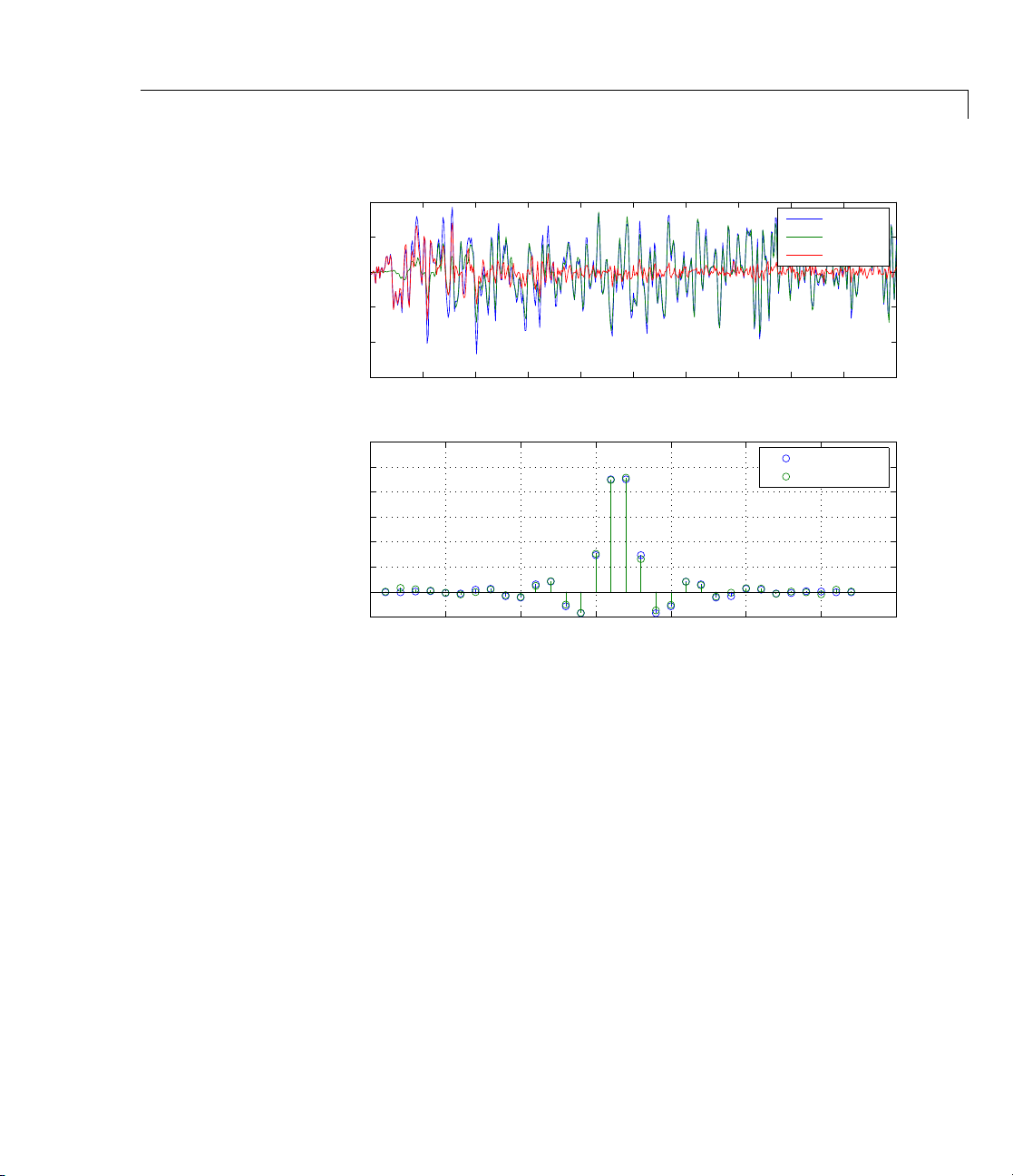
adaptfilt.dlms
2
1
0
−1
Signal Value
−2
−3
0 50 100 150 200 250 300 350 400 450 500
0.6
0.5
0.4
0.3
0.2
0.1
Coefficient Value
0
−0.1
0 5 10 15 20 25 30 35
System Identification of an FIR Filter
Time Index
Coefficient #
See Also adaptfilt.adjlms, adaptfilt.filtxlms, adaptfilt.lms
Desired
Output
Error
Actual
Estimated
References Shynk, J.J.,“Frequency-Domain and Multirate Adaptive Filtering,”
IEEE Signal Processing Magazine, vol. 9, no. 1, pp. 14-37, Jan. 1992.
2-47
Page 74

adaptfilt.fdaf
Purpose FIR adaptive filter that uses frequency-domain with bin step size
normalization
Syntax ha = adaptfilt.fdaf(l,step,leakage,delta,lambda,blocklen,
offset,...coeffs,states)
Description ha = adaptfilt.fdaf(l,step,leakage,delta,lambda,blocklen,
offset,...coeffs,states)
adaptive filter
inputargumentsyoucreateadefaultobjectwithl=10and
ha with bin step size normalization. If you omit all the
Input Arguments
Entries in the following table describe the input arguments for
adaptfilt.fdaf.
Input
Argument Description
l
step
leakage
delta
lambda
Adaptive filter length (the number of coefficients or
taps). l must be a positive integer; it defaults to 10
when you omi t the argument.
Step size of the adaptive filter. This is a scalar and
should lie in the range (0,1].
Leakage parameter of the adaptive filter. If this
parameter is set to a value between zero and one,
you implement a leaky FDAF algorithm.
defaults to 1 — no leakage provided in the algorithm.
Initial common value of all of the FFT input signal
powers. Its initial value should be positive.
defaults to 1.
Specifies the averaging factor used to compute the
exponentially-windowed FFT input signal powers for
the coefficient updates.
(0,1].
lambda defaults to 0.9.
constructs a frequency-domain FIR
step defaults to 1.
lambda should lie in the range
step =1.
leakage
delta
2-48
Page 75

Input
Argument Description
blocklen
offset
coeffs
states
Block length for the coefficient updates. This must be
a positive integer. For faster execution, (
l) should be a power of two.
Offset for the normalization terms in the coefficient
updates. Usethistoavoiddividebyzerosorbyvery
small numbers when any of the FFT input signal
powers become very small.
Initial time-domain coefficients of the adaptive filter.
coeff should be a length l vector. The adaptive
filter object uses these coefficients to compute the
initial frequency-domain filter coefficients via an FFT
computed after zero-padding the time-domain vector
by the
The adaptive filter states. states defaults to a zero
vector that has length equal to l.
blocklen.
adaptfilt.fdaf
blocklen +
blocklen defaults to l.
offset defaults to zero.
Properties Since your adaptfilt.fdaf filter is an object, it has properties that
define its behavior in operation. Note that many of the properties
are also input arguments for creating
show you the properties that apply, this table lists and describes each
property for the
adaptfilt.fdaf filter object.
adaptfilt.fdaf objects. To
2-49
Page 76

adaptfilt.fdaf
Name Range Description
Algorithm
None
Defines the adaptive filter
algorithm the object uses during
adaptation.
AvgFactor
(0, 1] S pecifies the averaging
factor used to compute the
exponentially-windowed FFT
input signal powers for the
coefficient updates. Same as the
input argument
BlockLength
Any integer Block length for the coefficient
updates. This must be a positive
integer. Forfasterexecution,
(
blocklen + l) should be a power
FFTCoefficients
of two.
Stores the discrete Fourier
blocklen defaults to l.
transform of the filter co efficients
in
coeffs.
FFTStates
FilterLength
Any
positive
States for the FFT operation.
Reports the length of the filter,
the number of coefficients or taps.
integer
Leakage
Leakage param eter of the
adaptive filter. if this parameter
issettoavaluebetweenzeroand
one, you implement a leaky FDAF
algorithm.
1—noleakageprovidedinthe
algorithm.
lambda.
leakage defaults to
2-50
Page 77

Name Range Description
Offset
PersistentMemory false or
Power
StepSize
Any
positive real
value
true
Any scalar
from zero
to one,
inclusive
Offset for the normalization
terms in the coefficient updates.
Use this to avoid dividing by
zero or by very small numbers
when any of the FFT input
signal powers become very small.
offset defaults to zero.
Determine whether the filter
states get restored to their
starting values for each
filtering operation. The starting
values are the values in place
when you create the filter.
PersistentMemory returns to
zero any state that the filter
changes during p rocessing.
States that the filter does not
change are not affected. Defaults
to
false.
Avectorof2*l elements, each
initialized with the value
from the input arguments. As you
filter data,
the filter process.
Specifies the step size taken
between filter coefficient updates
adaptfilt.fdaf
delta
Power gets updated by
Examples Quadrature Phase Shift Keying (QPSK) adaptive equalization using
1024 iterations of a 32-coefficient FIR filter. After this example code, a
figure demonstrates the equalization results.
2-51
Page 78

adaptfilt.fdaf
D = 16; % Number of samples of delay
b = exp(j*pi/4)*[-0.7 1]; % Numerator coefficients of channel
a = [1 -0.7]; % Denominator coefficients of channel
ntr= 1024; % Number of iterations
s = sign(randn(1,ntr+D))+j*sign(randn(1,ntr+D)); %QPSK signal
n = 0.1*(randn(1,ntr+D) + j*randn(1,ntr+D)); % Noise signal
r = filter(b,a,s)+n; % Received signal
x = r(1+D:ntr+D); % Input signal (received signal)
d = s(1:ntr); % Desired signal (delayed QPSK signal)
del = 1; % Initial FFT input powers
mu = 0.1; % Step size
lam = 0.9; % Averaging factor
ha = adaptfilt.fdaf(32,mu,1,del,lam);
[y,e] = filter(ha,x,d);
subplot(2,2,1); plot(1:ntr,real([d;y;e])); title('In-Phase Components');
legend('Desired','Output','Error');
xlabel('Time Index'); ylabel('signal value');
subplot(2,2,2); plot(1:ntr,imag([d;y;e])); title('Quadrature Components');
legend('Desired','Output','Error');
xlabel('Time Index'); ylabel('signal value');
subplot(2,2,3); plot(x(ntr-100:ntr),'.'); axis([-3 3 -3 3]);
title('Received Signal Scatter Plot'); axis('square');
xlabel('Real[x]'); ylabel('Imag[x]'); grid on;
subplot(2,2,4); plot(y(ntr-100:ntr),'.'); axis([-3 3 -3 3]);
title('Equalized Signal Scatter Plot'); axis('square');
xlabel('Real[y]'); ylabel('Imag[y]'); grid on;
2-52
Page 79

adaptfilt.fdaf
See Als
3
2
1
0
signal value
−1
−2
0 500 1000 1500
o
adaptf
adaptf
In−Phase Components
Time Index
Received Signal Scatter Plot
3
2
1
0
Imag[x]
−1
−2
−3
−2 0 2
Real[x]
ilt.ufdaf
ilt.blmsfft
Desired
Output
Error
1.5
1
0.5
0
−0.5
signal value
−1
−1.5
−2
, adaptfilt.pbfdaf, adaptfilt.blms,
Quadrature Components
Desired
Output
Error
0 500 1000 1500
3
2
1
0
Imag[y]
−1
−2
−3
Time Index
Equalized Signal Scatter Plot
−2 0 2
Real[y]
References Shynk, J.J.,“Frequency-Domain and Multirate Adaptive Filtering,”
IEEE Signal Processing Magazine, vol. 9, no. 1, pp. 14-37, Jan. 1992
2-53
Page 80

adaptfilt.filtxlms
Purpose FIR adaptive filter that uses filtered-x L M S
Syntax ha = adaptfilt.filtxlms(l,step,leakage,pathcoeffs,
pathest,...errstates,pstates,coeffs,states)
Description ha = adaptfilt.filtxlms(l,step,leakage,pathcoeffs,
pathest,...errstates,pstates,coeffs,states)
filtered-x LMS adaptive filter
Input Arguments
Entries in the following table describe the input arguments for
adaptfilt.filtxlms.
Input
Argument Description
l
step
leakage
pathcoeffs
pathest
fstates
Adaptive filter length (the number of coefficients or
taps) and it must be a positive integer.
to 10.
Filtered LMS step size. it must be a nonnegativ e
scalar.
is the filtered-x LMS leakage factor. it must be a
scalar between 0 and 1. If it is less than one, a leaky
version of
leakage defaults to 1 (no leakage).
is the secondary path filter model. this vector should
contain the coefficient values of the secondary path
from the output actuator to the error sensor.
is the estimate of the secondary path filter model.
pathest defaults to the values in pathcoeffs.
is a vector of filtered input states of the adaptive
filter.
equal to (
ha.
step defaults to 0.1.
adaptfilt.filtxlms is implemented.
fstates defaults to a zero vector of leng th
l -1).
constructs an
l defaults
2-54
Page 81

adaptfilt.filtxlms
Input
Argument Description
pstates
coeffs
states
Properties In the syntax for creating the adaptfilt object, the input options are
properties of the object created. This table lists the propertie s for the
adjoint LMS object, their default values, and a brief description of the
property.
are the secondary path FIR filter states. it must be
a vector of length equal to the (
-1).
pstates defaults to a vector of zeros of
length(pathcoeffs)
appropriate length.
is a vector of initial filter coefficients. it must be a
length
l vector. coeffs defaults to length l vector
of zeros.
Vector of initial filter states. states defaults
to a zero vector of length equal to the larger of
(
length(pathcoeffs)-1)and(length(pathest)-1).
Property
Algorithm
Coefficients
Default
Value Description
None
Defines the adaptive filter
algorithm the object uses
during adaptation
Vector of
elements
Vector containing the
initial filter coefficients. It
must be a length
where
l is the number of
filter coefficients.
defaults to length l vector
of zeros when you do not
provide the argument for
input.
l vector
coeffs
2-55
Page 82

adaptfilt.filtxlms
Property
FilteredInputStates l-1
FilterLength
States
SecondaryPathCoeffs
SecondaryPathEstimate pathcoeffs
SecondaryPathStates
StepSize
Default
Value Description
Vector of filtered input
states with length equal to
l -1.
Any positive
integer
Reports the length of
the filter, the number of
coefficients or taps
Vector of
elements
Vector of the adaptive
filter states.
states
defaults to a vector of zeros
which has length equal
to (
l + projectord -2)
No default A vector that contains the
coefficient values of your
secondary path from the
output actuator to the
error sensor
An estimate of the
values
secondary path filter
model
Vector of
size (
length
(pathcoeffs)
The states of the secondary
path FIR f ilter — the
unknown system
-1) with all
elements
equal to zero.
0.1
Sets the f iltered-x
algorithm step size
used for each iteration
of the adapting alg orithm.
Determines both how
quickly and how closely the
2-56
Page 83

adaptfilt.filtxlms
Default
Property
Example Demonstrate active noise control of a random noise signal over 1000
iterations.
As the figure that follows this code demonstrates, the filtered-x LMS
filter successfully controls random noise in this context.
x = randn(1,1000); % Noise source
g = fir1(47,0.4); % FIR primary path system model
n = 0.1*randn(1,1000); % Observation noise signal
d = filter(g,1,x)+n; % Signal to be cancelled
b = fir1(31,0.5); % FIR secondary path system model
mu = 0.008; % Filtered-X LMS step size
ha = adaptfilt.filtxlms(32,mu,1,b);
[y,e] = filter(ha,x,d); plot(1:1000,d,'b',1:1000,e,'r');
title('Active Noise Control of a Random Noise Signal');
legend('Original','Attenuated');
xlabel('Time Index'); ylabel('Signal Value'); grid on;
Value Description
adaptive filter converges
to the filter solution.
2-57
Page 84
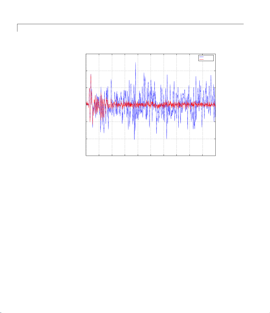
adaptfilt.filtxlms
3
2
1
0
Signal Value
−1
−2
−3
0 100 200 300 400 500 600 700 800 900 1000
Active Noise Control of a Random Noise Signal
Time Index
Original
Attenuated
See also adaptfilt.dlms, adaptfilt.lms
References Kuo, S.M., and Morgan, D.R. Active Noise Control Systems: Algorithms
and DSP Implementations,NewYork,N.Y:JohnWiley&Sons,1996.
2-58
Widrow, B., and Stearns, S.D. Adaptive Signal Processing,Upper
Saddle River, N.J: Prentice Hall, 1985.
Page 85

adaptfilt.ftf
Purpose Fast transversal LMS adaptive filter
Syntax ha = adaptfilt.ftf(l,lambda,delta,gamma,gstates,coeffs,
states)
Description ha = adaptfilt.ftf(l,lambda,delta,gamma,gstates,coeffs,
states)
object
Input Arguments
Entries in the following table describe the input arguments for
adaptfilt.ftf.
Input
Argument Description
l
lambda
delta
gamma
gstates
coeffs
states
constructs a fast transversal least squares adaptive filter
ha.
Adaptive filter length (the number of coefficients or
taps) and it must be a positive integer.
to 10.
RLS forgetting factor. This is a scalar that should
lie in the range (1-0.5/
Soft-constrained initialization factor. This scalar
should be positive and sufficiently large to prevent
an excessive number of Kalman gain rescues.
defaults to one.
Conversion factor. gamma defaults to one specifying
soft-constrained initialization.
States of the Kalman gain updates. gstates
defaults to a zero vector of length l.
Length l vector of initial filter coefficients. coeffs
defaults to a length
Vector of initial filter States. states defaults to a
zero vector of length (
l,1]. lambda defaults to 1.
l vector of zeros.
l-1).
l defaults
delta
2-59
Page 86

adaptfilt.ftf
Properties Since your adaptfilt.ftf filter is an object, it has properties that
define its operating behavior. N ote that many of the properties are also
input arguments for creating
properties that apply, this table lists and describes each property for
the fast transversal least squares filter object.
Name Range Description
Algorithm
BkwdPrediction
Coefficients
ConversionFactor
FilterLength
ForgettingFactor
adaptfilt.ftf objects. To show you the
None
Vector of
elements
Any
positive
integer
Defines the adaptive filter
algorithm the object uses during
adaptation
Returns the predicted samples
generated during adaptation.
Refer to [2] in the bibliography
for details about linear
prediction.
Vector containing the initial
filter coefficients. It must be a
length
number of filter coefficients.
coeffs defaults to length l
vector of zeros when you do not
provide the argument for input.
Conversion factor. Called gamma
when it is an input argument,
it defaults to the matrix [1 -1]
that specifies soft-constrained
initialization.
Reports the length of the filter,
the number of coefficients or taps
RLS forgetting factor. This
is a scalar that should lie in
the range (1-0.5/
defaults to 1.
l vector where l is the
l,1]. lambda
2-60
Page 87

Name Range Description
FwdPrediction
Contains the predicted values
for samples du rin g adaptation.
Compare these to the actual
samples to get the error and
power.
InitFactor
Soft-constrained initialization
factor. This scalar should be
positive and sufficiently large
to prevent an excessive number
of Kalman gain rescues.
defaults to one.
KalmanGain
Empty when you construct the
object, this gets populated after
you run the filter.
PersistentMemory false or
true
Determine whether the filter
states get restored to their
starting values for each filtering
operation. The starting values
arethevaluesinplacewhen
you create the filter if you
have not changed the filter
since you constructed it.
PersistentMemory returns to
zero any state that the filter
changes during processing.
States that the filter does not
change are not affected. Defaults
to
false.
States
Vector of
elements,
data type
double
Vector of the adaptive filter
states.
states defaults to a
vector of zeros which has length
equal to (
l + projectord -2).
adaptfilt.ftf
delta
2-61
Page 88

adaptfilt.ftf
Examples System Identification of a 32-coefficient FIR filter by running the
identification process for 500 iterations.
x = randn(1,500); % Input to the filter
b = fir1(31,0.5); % FIR system to be identified
n = 0.1*randn(1,500);% Observation noise signal
d = filter(b,1,x)+n; % Desired signal
N = 31; % Adaptive filter order
lam = 0.99; % RLS forgetting factor
del = 0.1; % Soft-constrained initialization factor
ha = adaptfilt.ftf(32,lam,del);
[y,e] = filter(ha,x,d);
subplot(2,1,1); plot(1:500,[d;y;e]);
title('System Identification of an FIR Filter');
legend('Desired','Output','Error');
xlabel('Time Index'); ylabel('signal value');
subplot(2,1,2); stem([b.',ha.Coefficients.']);
legend('Actual','Estimated'); grid on;
xlabel('coefficient #'); ylabel('Coefficient Value');
2-62
For this example of identifying an unknown system, the figure shows
that the adaptation process identifies the filter coefficients for the
unknown FIR filter within the first 150 iterations.
Page 89

adaptfilt.ftf
0
2
1
0
−1
signal value
−2
−3
0 50 100 150 200 250 300 350 400 450 50
0.6
0.5
0.4
0.3
0.2
0.1
Coefficient Value
0
−0.1
0 5 10 15 20 25 30 35
System Identification of an FIR filter
Desired
Output
Error
Time Index
Actual
Estimated
coefficient #
See Also adaptfilt.swftf, adaptfilt.rls, adaptfilt.lsl
References D.T.M. Slock and Kailath, T., “Numerically Stable Fast Transversal
Filters for Recursive Least Squares Adaptive Filtering,” IEEE Trans.
Signal Processing, vol. 38, no. 1, pp. 92-114.
2-63
Page 90

adaptfilt.gal
Purpose FIR adaptive filter that uses gradient lattice
Syntax ha = adaptfilt.gal(l,step,leakage,offset,rstep,delta,
lambda,...rcoeffs,coeffs,states)
Description ha = adaptfilt.gal(l,step,leakage,offset,rstep,delta,
lambda,...rcoeffs,coeffs,states)
lattice FIR filter
ha.
Input Arguments
Entries in the following table describe the input arguments for
adaptfilt.gal.
Input
Argument Description
l
step
leakage
offset
Length of the joint process filter coefficients. It must
be a positive integer and must be equal to the length
of the reflection c oefficients plus one.
Joint process step siz e of the adaptive filter. This
scalar should be a value between zero and one.
defaults to 0.
Leakage factor of the adaptive filter. It must be a
scalar be tween 0 and 1. Setting lea k age less than one
implements a leaky algorithm to estimate both the
reflection and the joint process coefficients.
defaults to 1 (no leakage).
Specifies an optional offset for the denominator of
thestepsizenormalizationterm. Itmustbeascalar
greaterorequaltozero. Anon-zero
to avoid divide-by-near-zero conditions when the input
signal amplitude becomes very small.
to 1.
constructs a gradient adaptive
l defaults to 10.
step
leakage
offset is useful
offset defaults
2-64
Page 91

Input
Argument Description
rstep
Reflection process step size of the adaptive filter. This
scalar should be a value between zero and one.
defaults to step.
delta
Initial common value of the forward and backward
prediction error powers. It should be a positive value.
0.1 is the default value for
lambda
Specifies the averaging factor used to compute the
exponentially windowed forward and backward
prediction error p ow ers for the coefficient update s.
lambda should lie in the range (0, 1]. lambda defaults
to the value (1 -
rcoeffs
Vector of initial reflection coefficients. It should be a
length (l-1) vector.
coeffs
of length (
Vector of initial joint process filter coefficients. It
l-1).
must be a length
l vector of zeros.
states
Vector of the backward prediction error states of the
adaptive filter.
length (
l-1).
adaptfilt.gal
rstep
delta.
step).
rcoeffs defaults to a zero vector
l vector. coeffs defaults to a length
states defaults to a zero vector of
Properties Since your adaptfilt.gal filter is an object, it has properties that
define its behavior in operation. Note that many of the properties are
also input arguments for creating
the properties that apply, this table lists and describes each property
for the affine projection filter object.
adaptfilt.gal objects. To show you
2-65
Page 92

adaptfilt.gal
Name Range Description
Algorithm
None
Defines the adaptive filter
algorithm the object uses during
adaptation
AvgFactor
Specifies the averaging
factor used to compute the
exponentially-windowed forward
and backward prediction error
powers for the coefficient
updates. Same as the input
BkwdPredErrorPower
argument
Returns the minimum
lambda.
mean-squared prediction error.
Refer to [2] in the bibliography
for details about linear prediction
Coefficients
Vector of
elements
Vector containing the initial filter
coefficients. It must be a length
l vector where l is the number
of filter coefficients.
defaults to length l vector of
zeros when you do not provide
the argument for input.
FilterLength
Any
positive
Reports the length of the filter,
the number of coefficients or taps
integer
FwdPredErrorPower
Returns the minimum
mean-squared pre diction error in
the forward direction. Refer to
[2] in the bibliography for details
about linear prediction.
coeffs
2-66
Page 93

Name Range Description
Leakage
0to1
Leakage parameter of the
adaptive filter. If this parameter
issettoavaluebetweenzeroand
one, you implement a leaky GAL
algorithm.
1—noleakageprovidedinthe
algorithm.
Offset
Offset for the normalization
terms in the coefficient updates.
Use this to avoid dividing by zero
or by very small numbers when
input signal amplitude becomes
very small.
one.
PersistentMemory false or
true
Determine whether the filter
states get restored to their
starting values for each filtering
operation. The starting values
are the values in place when
you create the filter if you
have not changed the filter
since you constructed it.
PersistentMemory returns to
zero any state that the filter
changes during processing.
States that the filter does not
change are not affected. Defaults
to
false.
ReflectionCoeffs
Coefficients determined for the
reflection portion of the filter
during adaptation.
adaptfilt.gal
leakage defaults to
offset defaults to
2-67
Page 94

adaptfilt.gal
Name Range Description
ReflectionCoeffsStep
States
Vector of
elements
StepSize
0to1
Examples Perform a Quadrature Phase Shift Keying (QPSK) adaptive e qualiza tion
using a 32-coefficient adaptive filter over 1000 iterations.
D = 16; % Number of delay samples
b = exp(j*pi/4)*[-0.7 1]; % Numerator coefficients
a = [1 -0.7]; % Denominator coefficients
ntr= 1000; % Number of iterations
s = sign(randn(1,ntr+D)) + j*sign(randn(1,ntr+D)); % QPSK signal
n = 0.1*(randn(1,ntr+D) + j*randn(1,ntr+D)); % Noise signal
r = filter(b,a,s)+n; % Received signal
x = r(1+D:ntr+D); % Input signal (received signal)
d = s(1:ntr); % Desired signal (delayed QPSK signal)
L = 32; % filter length
mu = 0.007; % Step size
ha = adaptfilt.gal(L,mu);
[y,e] = filter(ha,x,d);
subplot(2,2,1); plot(1:ntr,real([d;y;e]));
title('In-Phase Components');
legend('Desired','Output','Error');
xlabel('Time Index'); ylabel('signal value');
subplot(2,2,2); plot(1:ntr,imag([d;y;e]));
title('Quadrature Components');
legend('Desired','Output','Error');
xlabel('Time Index'); ylabel('Signal Value');
Size of the steps used to
determine the reflection
coefficients.
Vectoroftheadaptivefilter
states.
states defaults to a
vector of zeros which has length
equal to (
l + projectord -2).
Specifies the step size taken
between filter coefficient u pdate s
2-68
Page 95

subplot(2,2,3); plot(x(ntr-100:ntr),'.'); axis([-3 3 -3 3]);
title('Received Signal Scatter Plot'); axis('square');
xlabel('Real[x]'); ylabel('Imag[x]'); grid on;
subplot(2,2,4); plot(y(ntr-100:ntr),'.');
axis([-3 3 -3 3]); title('Equalized Signal Scatter Plot');
axis('square'); xlabel('Real[y]'); ylabel('Imag[y]'); grid on;
To see the results, look at this figure.
adaptfilt.gal
1.5
1
0.5
0
signal value
−0.5
−1
−1.5
In−Phase Components
Desired
Output
Error
0 200 400 600 800 1000
3
2
1
0
Imag[x]
−1
−2
−3
Time Index
Received Signal Scatter Plot
−2 0 2
Real[x]
1.5
0.5
Signal Value
−0.5
−1
−1.5
Quadrature Components
1
0
0 200 400 600 800 1000
3
2
1
0
Imag[y]
−1
−2
−3
Time Index
Equalized Signal Scatter Plot
−2 0 2
Real[y]
Desired
Output
Error
See Also adaptfilt.qrdlsl, adaptfilt.lsl, adaptfilt.tdafdft
References Griffiths, L.J. “A Continuously Adaptive Filter Implemented as a
Lattice Structure,” Proc. IEEE Int. C onf. on Acoustics, Speech, and
Signal Processing, Hartford, CT, pp. 683-686, 1977
2-69
Page 96

adaptfilt.gal
Haykin, S.,Adaptive Filter Theory, 3rd Ed., Upper Saddle River, NJ,
Prentice Hall, 1996
2-70
Page 97

adaptfilt.hrls
Purpose FIR adaptive filter that uses householder (RLS)
Syntax ha = adaptfilt.hrls(l,lambda,sqrtinvcov,coeffs,states)
Description ha = adaptfilt.hrls(l,lambda,sqrtinvcov,coeffs,states)
constructs an FIR householder RLS adaptive filter ha.
Input Arguments
Entries in the following table describe the input arguments for
adaptfilt.hrls.
Input
Argument Description
l
lambda
sqrtinvcov
coeffs
states
Adaptive filter length (the number of coefficients or
taps) and it must be a positive integer.
to 10.
RLS forgetting factor. This is a scalar and should
lie in the range (0, 1].
the adaptation process retains infinite memory.
Square-root of the inverse of the sliding w ind ow
input signal covariance matrix. This square matrix
should be full-ranked.
Vector of initial filter coefficients. It must be a
length
vector of zeros.
Vector of initial filter states. It must be a length
l-1 vector. states defaults to a length l-1 vector
of zeros.
l vector. coeffs defaults to being a length l
lambda defaults to 1 meaning
l defaults
Properties Since your adaptfilt.hrls filter is an object, it has properties that
define its behavior in operation. Note that many of the properties are
also input arguments for creating
the properties that apply, this table lists and describes each property
for the affine projection filter object.
adaptfilt.hrls objects. To show you
2-71
Page 98

adaptfilt.hrls
Name Range Description
Algorithm
None
Defines the adaptive filter
algorithm the object us es during
adaptation
Coefficients
Vector of
elements
Vector containing the initial
filter coefficients. It must be a
length
l vector where l is the
numberoffiltercoefficients.
coeffs defaults to length l
vector of zeros when you do not
provide the argument for input.
FilterLength
Any
positive
Reports the length of the filter,
the number of coefficients or taps
integer
ForgettingFactor
Scalar RLS forgetting factor. Thi s is a
scalar and should lie in the range
(0, 1]. Same as input argument
lambda. It defaults to 1 meaning
the adaptation process retains
infinite memory.
KalmanGain
Vector of
size (
l,1)
Empty when you construct the
object, this gets populated after
you run the filter.
2-72
Page 99

Name Range Description
PersistentMemory false or
true
Determine whether the filter
states get restored to the ir
starting values for each filtering
operation. The starting values
are the values in place when
you create the filter if you
have not changed the filter
since you constructed it.
PersistentMemory returns to
zero any state that the filter
changes during processing.
Defaults to
SqrtInvCov
Matrix of
doubles
Square root of the inverse of
the sliding window input signal
covariance matrix. T his square
matrix should be full-ranked.
States
Vector of
elements,
data type
double
Vector of the adaptive filter
states.
states defaults to a
vector of zeros which has length
equal to (
l -1).
adaptfilt.hrls
false.
Examples Use 500 iterations of an adaptive filter object to identify a 32-coefficient
FIR filter system. Both the example code and the resulting figure show
the successful filter identification through adaptive filter processing.
x = randn(1,500); % Input to the filter
b = fir1(31,0.5); % FIR system to be identified
n = 0.1*randn(1,500); % Observation noise signal
d = filter(b,1,x)+n; % Desired signal
G0 = sqrt(10)*eye(32); % Initial sqrt correlation matrix inverse
lam = 0.99; % RLS forgetting factor
ha = adaptfilt.hrls(32,lam,G0);
[y,e] = filter(ha,x,d);
subplot(2,1,1); plot(1:500,[d;y;e]);
2-73
Page 100

adaptfilt.hrls
title('System Identification of an FIR Filter');
legend('Desired','Output','Error');
xlabel('Time Index'); ylabel('Signal Value');
subplot(2,1,2); stem([b.',ha.Coefficients.']);
legend('Actual','Estimated'); grid on;
xlabel('Coefficient #'); ylabel('Coefficient Value');
3
2
1
0
Signal Value
−1
−2
0 50 100 150 200 250 300 350 400 450 500
0.6
0.5
0.4
0.3
0.2
0.1
Coefficient Value
0
−0.1
0 5 10 15 20 25 30 35
System Identification of an FIR filter
Time Index
Coefficient #
See Also adaptfilt.hswrls, adaptfilt.qrdrls, adaptfilt.rls
Desired
Output
Error
Actual
Estimated
2-74
 Loading...