Mathworks ECONOMETRICS TOOLBOX 1 user guide

Download

Econometrics Tool

User’s Guide

box™ 1

How to Contact The MathWorks

www.mathworks. comp.soft-sys.matlab Newsgroup www.mathworks.com/contact_TS.html T echnical Support

suggest@mathworks.com Product enhancement suggestions

bugs@mathwo doc@mathworks.com Documentation error reports service@mathworks.com Order status, license renewals, passcodes

info@mathwo

com

rks.com

Web

Bug reports

Sales, prici

ng, and general information

508-647-7000 (Phone)

508-647-7001 (Fax)

The MathWorks, Inc. 3 Apple Hill Drive Natick, MA 01760-2098

For contact information about worldwide offices, see the MathWorks Web site.

Econometrics Toolbox™ User’s Guide

The software described in this document is furnished under a license agreement. The software may be used or copied only under the terms of the license agreement. No part of this manual may be photocopied or reproduced in any form without prior written consent from The MathW orks, Inc.

FEDERAL ACQUISITION: This provision applies to all acquisitions of the Program and Documentation by, for, or through the federal government of the United States. By accepting delivery of the Program or Documentation, the government hereby agrees that this software or documentation qualifies as commercial computer software or commercial computer software documentation as such terms are used or defined in FAR 12.212, DFARS Part 227.72, and DFARS 252.227-7014. Accordingly, the terms and conditions of this Agreement and only those rights specified in this Agreement, shall pertain to and govern theuse,modification,reproduction,release,performance,display,anddisclosureoftheProgramand Documentation by the federal government (or other entity acquiring for or through the federal government) and shall supersede any conflicting contractual terms or conditions. If this License fails to meet the government’s needs or is inconsistent in any respect with federal procurement law, the government agrees to return the Program and Docu mentation, unused, to The MathWorks, Inc.

Trademarks

MATLAB and Simulink are registered trademarks of The MathWorks, Inc. See

www.mathworks.com/trademarks for a list of additional trademarks. Other product or brand

names may be trademarks or registered trademarks of their respective holders.

Patents

The MathWorks products are protected by one or more U.S. patents. Please see

www.mathworks.com/patents for more information.

Revision History

October 2008 Online only Version 1.0 (Release 2008b) March 2009 Online only Revised for Version 1.1 (Release 2009a) September 2009 Online only Revised for Version 1.2 (Release 2009b) March 2010 Online only Revised for Version 1.3 (Release 2010a)

Getting Started

Product Overview ................................. 1-2

Contents

Technical Conventions

Time Series Arrays Conditional vs. Unconditional Variance Prices, Returns, and Compounding Stationary and Nonstationary Time Series

Time Series Modeling

Characteristics of Time Series Forecasting Time Series Serial Dependence in Innovations Conditional Mean and Variance Models GARCH Models

................................... 1-12

............................. 1-3

................................ 1-3

............... 1-3

................... 1-4

............. 1-4

.............................. 1-7

....................... 1-7

............................ 1-9

.................... 1-10

............... 1-11

Example Workflow

Estimation ........................................ 2-2

Forecasting

....................................... 2-4

Simulation

Analysis

........................................ 2-5

.......................................... 2-7

iii

Model Selection

Specification Structures ........................... 3-2

About Specification Structures Associating Model E quation Variables with Corresponding

Parameters in Specification Structures Working with Specification Structures Example: Specif ica t io n Structures

....................... 3-2

.............. 3-4

................ 3-5

.................... 3-9

Model Identification

Autocorrelation and Partial Autocorrelation Unit Root Tests Misspecification Tests Akaike and Bayesian Information

Model Construction

Setting Model Parameters Setting Equality Constraints

Example: Model Selection

............................... 3-11

............ 3-11

................................... 3-11

.............................. 3-30

.................... 3-43

................................ 3-46

.......................... 3-46

........................ 3-50

.......................... 3-54

Simulation

Process Simulation ................................ 4-2

Introduction Preparing th e Example Data Simulating Single Paths Simulating Multiple Paths

...................................... 4-2

........................ 4-2

............................ 4-3

.......................... 4-5

iv Contents

Presample Data

About Presample Data Automatically Generating Presample Data Running Simulations With User-Specified Presample

Data

.......................................... 4-11

................................... 4-6

............................. 4-6

............ 4-6

Estimation

Maximum Likelihood Estimation .................... 5-2

Estimating Initial Parameters

Computing User-Specified In itial E stimates Computing Automatically Generated Initial Estimates Working With Parameter Bounds

Presample Data

Calculating Presample Data Using the garchfit Function to Generate User-Specified

Presample Observations

Automatically Generating Presample Observations

Optimization Termination

Optimization Parameters Setting Maximum Numbers of Iterations and Function

Evaluations Setting Function Termination Tolerance Enabling Estimation Convergence Setting Constraint Violation Tolerance

Examples

Presample Data Inferring Residuals Estimating ARMA(R,M) Parameters Lower Bound Constraints

......................................... 5-21

................................... 5-12

.................................... 5-15

................................... 5-21

................................ 5-24

...................... 5-4

............ 5-4

.................... 5-10

......................... 5-12

.......................... 5-12

.......................... 5-15

........................... 5-15

............... 5-16

.................... 5-17

................ 5-18

.................. 5-30

........................... 5-31

... 5-6

...... 5-13

Forecasting

MMSE Forecasting ................................. 6-2

About the Forecasting Engine Computing the Conditional Standard Deviations of Future

Innovations

.................................... 6-2

....................... 6-2

Computing the Conditional Mean Forecasting of the Return

Series MMSE Volatility Forecasting of Returns Approximating Confidence Intervals Associated with

Conditional Mean Forecasts Using the Matrix of Root

Mean Square Errors (RMSE)

......................................... 6-3

.............. 6-3

...................... 6-4

Presample Data

Asymptotic Behavior

Examples

Forecasting Using GARCH Predictions Forecasting Multiple Periods Forecasting Multiple Realizations

......................................... 6-9

................................... 6-6

............................... 6-7

................ 6-9

........................ 6-12

.................... 6-15

Regression

Introduction ...................................... 7-2

Regression in Estimation

Fitting a Return Series Fitting a Regression M odel to a Return Series

Regression in Simulation

........................... 7-3

............................. 7-3

.......... 7-5

........................... 7-8

vi Contents

Regression in Forecasting

Using Forecasted Explanatory Data Generating Forecasted Explanatory Data

Regression in Monte Carlo

Ordinary Least Squares Regression

.......................... 7-9

......................... 7-11

.................. 7-9

.............. 7-10

................. 7-12

Multiple Time Series

Multiple Time Series Models ........................ 8-2

Types of Multiple Time Series Models Lag Operator Representation Stable and Invertible Models

........................ 8-3

........................ 8-4

................. 8-2

Modeling Multiple Time Series

A Generic Workflow

Multiple Time Series Data Structures

Introduction to Multiple Time Series Data Response Data Structure Exogenous Data Structure Example: Response Data Structure Example: Exogenous Data Structure Data Preproces sing Partitioning Response Data Seemingly Unrelated Regression for Exogenous Da ta

Creating Model Specification Structures

Models for Multiple Time Series Specifying Models Defining a Model Specification Structure with Known

Parameters

Defining a Model Specification Structure with No

Parameter Values

Defining a Model Specification Structure with Selected

Parameter Values

Displaying an d Changing a Model Sp ecifica tion

Structure

Determining an Appropriate Number of Lags

...................................... 8-22

............................... 8-5

................................ 8-12

................................. 8-16

.................................... 8-17

............................... 8-19

............................... 8-20

...................... 8-5

............... 8-7

............. 8-7

........................... 8-8

.......................... 8-8

................... 8-10

.................. 8-11

......................... 8-13

............ 8-16

..................... 8-16

........... 8-23

.... 8-14

Fitting Parameters

Preparing Models for Fitting Including Exogenous Data Converting Betw ee n Models Fitting Models to Data Examining the Stability of a Fitted Model

................................ 8-25

........................ 8-25

.......................... 8-26

......................... 8-26

............................. 8-31

............. 8-37

vii

Forecasting, Simulating, and Analyzing Models ...... 8-38

Forecasting with Multiple Time Series Models Returning to Original Scaling Calculating Impulse Responses with vgxproc

....................... 8-44

.......... 8-38

........... 8-44

Multiple Time Series Case Study

Overview o f the Case Study Loading and Transforming Data Selecting and Fitting Models Checking Model Adequacy Forecasting

...................................... 8-58

.......................... 8-53

.................... 8-47

......................... 8-47

..................... 8-47

........................ 8-51

Lag Operator Polynomials

Creating a Lag Operator Object ..................... 9-2

Simple Second-Degree Polynomial

ARMA(2,1) Model

Impulse Response Monte Carlo Simulation

ARIMA(2,1,1) Model

.................................. 9-7

................................. 9-9

............................ 9-11

................................ 9-12

.................. 9-4

viii Contents

Seasonal ARIMA Model

Time Series Filtering and Initial Conditions

Polynomial Division

Univariate Polynomial Inversion Multivariate Polynomial Inve rsion Transformation of VAR M odels

............................ 9-15

............................... 9-20

..................... 9-20

................... 9-24

...................... 9-25

......... 9-18

Stochastic Differential Equations

Introduction ...................................... 10-2

SDE Modeling Trials vs. Paths NTRIALS, NPERIODS, and NSTEPS

.................................... 10-2

................................... 10-3

................. 10-4

SDE Class Hierarchy

SDE Objects

Introduction Creating SDE Objects Modeling with SDE Objects

SDE Methods

Example: Simulating Equity Prices

Simulating Multidimensional Market Models Inducing Dependence and Correlation DynamicBehaviorofMarketParameters Pricing Equity Options

Example: Simulating Interest Rates

Simulating Interest Rates Ensuring Positive Interest Rates

Example: Stratified Sampling

Performance Considerations

Managing Memory Enhancing Performance Optimizing Accuracy: About Solution Precis ion and

Error

....................................... 10-8

...................................... 10-8

...................................... 10-31

......................................... 10-75

............................... 10-5

.............................. 10-8

......................... 10-16

................. 10-32

................. 10-44

.............. 10-47

............................. 10-53

................. 10-56

.......................... 10-56

..................... 10-62

....................... 10-67

....................... 10-73

................................ 10-73

............................ 10-74

.......... 10-32

Function Reference

Data Preprocessing ................................ 11-2

GARCH Modeling

Model Specification

Model Visualization

Multiple Time Series

Lag Operator Polynomials

Statistics and Tests

Stochastic Differential Equations

Utilities

........................................... 11-7

.................................. 11-2

................................ 11-2

............................... 11-3

.......................... 11-3

................................ 11-4

................... 11-6

x Contents

Functions — Alphabetical List

Data Sets, Demos, and Example Functions

Bibliography

Examples

Getting Started .................................... C-2

Example Workflow

Model Selection

Simulation

Estimation

Forecasting

Regression

Multiple Time Series

Lag Operator Polynomial

........................................ C-2

........................................ C-3

....................................... C-3

........................................ C-3

................................. C-2

................................... C-2

............................... C-3

........................... C-4

Stochastic Differential Equations ................... C-4

Glossary

Index

xii Contents

Getting Started

• “Product Overview” on page 1-2

• “Technical Conventions” on page 1-3

• “Time Series Modeling” on page 1-7

1 Getting Started

Product Overview

The Econometrics Toolbox™ software, combined with MATLAB®, Optimization Toolbox™, and Statistics Toolbox™ software, provides an integrated computing environment for modeling and analyzing economic and social systems. It enables economists, quantitative analysts, and social scientists to perform rigorous modeling, simulation, calibration, identification, and f orecasting with a variety of standard econometrics too ls.

Specific functionality includes:

• Univariate ARMAX/GARCH composite models with several GARCH

• Dickey-Fuller and Phillips-Perron unit root tests

• Multivaria te VARX model estimation, simulation, and forecasting

• Multivariate VARMAX model simulation and forecasting

• Monte Carlo simulation of many common stochastic differential equations

variants (ARCH/GARCH, EGARCH, and GJR)

(SDEs), including arithmetic and geometric Brownian motion, Constant Elasticity of Variance (CEV), Cox-Ingersoll-Ross (CIR), Hull-White, Vasicek, and Heston stochastic volatility

1-2

• Monte Carlo simulation support for virtually any linear or nonlinear SDE

• Hodrick-Prescott filter

• Statistical tests such as likelihood ratio, Engle’s ARCH, Ljung-Box Q

• Diagnostic tools such as Akaike information criterion (AIC), Bayesian

information criterion (BIC), and partial/auto/cross correlation functions

• Lagoperatorobjectsfordatafiltering and time series modeling

Technical Conventions

In this section...

“Time Series Arrays” on page 1-3 “Conditional vs. Uncondition al Variance” on page 1-3 “Prices, Returns, and Compounding” on page 1-4 “Stationary and Nonstationary Time Series” on page 1-4

Tip For information on economic modeling terminology, see the “Glossary” on page Glossary-1.

Time Series Arrays

A time series is an ordered set of observations stored in a MATLAB array. The rows of the array correspond to time-tagged indices, or observations, and the columns correspond to sample paths, independent realizations, or individual time series. In any given column, the first row contains the oldest observation and the last row contains the most recent observation. In this representation, a time series array is column-oriented.

Technical Conventions

Note Some Econometrics Toolbox functions can process univariate time series arrays formatted as either row or column vectors. However, many functions now strictly enforce the column-oriented representation of a time series. To avoid ambiguity, format single realizations of univariate time series as column vectors. Representing a time series in column-oriented format avoids misinterpretation of the arguments. It also makes it easier for you to display data in the MATLAB Command Window.

Conditional vs. Unconditional Variance

The term conditional implies explicit dependence on a past sequence of observations. The term unconditional applies more to long-term behavior of a time series, and assumes no explicit knowledge of the past. Time series typically modeled by Econometrics Toolbox software have constant means

1-3

1 Getting Started

and unconditional variances but non-constant conditional variances (see “Stationary a nd Nonstationary Time Series” on page 1-4).

Prices, Returns, and Compounding

The Econometrics T oolbox software assumes that time series vectors and matrices are time-tagged series of observations, usually of returns. The toolbox lets you convert a price series to a return series with either continuous compounding or simple periodic compounding, using the

price2ret function.

If you denote successive price observations made at times t and t+1 as P and P into a return series {y

, respectively, continuous compounding transforms a price series {Pt}

t+1

==−

log log log

}using

Simple periodic compounding uses the transformation

PPPP

−

++11

tttt

=−

(1-1)

Continuous compounding is the default Econometrics Toolbox compounding method, and is the preferred method for most of continuou s-tim e finance. Since modeling is typically based o n relatively high frequency data (daily or weekly observations), the difference between the two methods is usually small. Howeve r, some toolbox functions produce results that are approximate for simple periodic compounding, but exact for continuous compounding. If you adopt the continuous compounding default convention when moving between prices and returns, all toolbox functions produce exact results.

Stationary and Nonstationary Time Series

The Econometrics Toolbox software assumes that return series ytare covariance-stationary processes, with constant mean and constant

unconditional variance. Variances conditional on the past, such as V(y are considered to be random variables.

t|yt–1

1-4

Technical Conventions

The price-to-return transformation generally guarantees a stable data set for modeling. For example, the following figure illustrates an equity price series. It shows daily closing values of the NASDAQ Composite Index. There appears to be no long-run average level about which the series evolves, indicating a nonstationary time series.

The following figure illustrates the continuously compounded returns associated with the same price series. In contrast, the returns appear to have a stable mean over time.

1-5

1 Getting Started

1-6

Time Series Modeling

In this section...

“Characteristics of Time Series” on page 1-7 “Forecasting Time Series” on page 1-9 “Serial Dependence in Innovations” on page 1-10 “Conditional Mean and Variance Models” on page 1-11 “GARCH Models” on page 1-12

Characteristics of Time Series

Econometric models are designed to capture characteristics that are commonly associated with time series, including fat tails, volatility clustering, and leverage effects.

Probability distributions for asset returns often exhibit fatter tails than the standard normal distribution. The fat tail phenomenon is called excess kurtosis. Time series that exhib it fat tails are often called leptokurtic.The dashed red line in the following figure illustrates excess kurtosis. The solid blue line shows a normal distribution.

Time Series Modeling

1-7

1 Getting Started

1-8

Time serie s also often exhibit volatility clustering or persistence. In volatility clustering, large changes tend to follow large changes, and small changes tend to follow small changes. T he changes from one period to the next are typically of unpredictable sign. Large disturbances, po sitive or negative, become part of the information set used to construct the variance forecast of the next period’s disturbance. In this way, large shocks of either sign can persist and influence volatility forecasts for several periods.

Volatility clustering suggests a time series model in which successive disturbances are uncorrelated but serially dependent. Th e following figure illustrates this characteristic. It shows the daily returns of the New York Stock Exchange Com posite Index.

Time Series Modeling

Volatility clustering, which is a type of heteroscedasticity, accounts for some of the excess kurtosis typically observed in financial data. Part of the excess kurtosis can also result from the presence of non-normal asset return distributions that happen to have fat tails. An example of such a distribution is Student’s t.

Certain classes of asymmetric GARCH m odels can also capture the leverage effect. This effect results in observed asset returns being negatively correlated with changes in volatility. For certain asset classes, volatility tends to rise in response to lower than expected returns and to fall in response to higher than expected returns. Such an effect suggests GARCH models that include an asymmetric response to positive and negative impulses.

Forecasting Time Series

You can treat a time series as a sequence of random observations. This random sequence, or stochastic process, may exhibit a degree of correlation from one observation to the next. You can use this correlation structure to

1-9

1 Getting Started

predict future values of the process based on the past history of observations. Exploiting the correlation structure, if any , allows you to decompose the time series into the following components:

• A deterministic component (the forecast)

• A random component (the error, or uncertainty, associated with the

forecast)

The f ollow ing represents a univariate model of an observed time series:

yft X

=− +(,)1



In this model,

• f(t –1,X) is a nonlinear function representing the forecast, or deterministic component, of the current return as a function of information known at time t – 1. The forecast includes:

{}

- Past disturbances



, ,...

tt−−12

1-10

{}

- Past observations

, ,...

tt−−12

- Any other relevant explanatory time series data, X

}isarandominnovations process. It represents disturbances in the m ean

• {ε

of {y

}. You can also interpret εtas the single-period-ahead forecast error.

Serial Dependence in Innovations

A common assumption when modeling time series is that the forecast errors (innovations) are zero-mean random disturbances that are uncorrelated from one period to the next.

Although successive innovations are uncorrelated, they are not independent. In fact, an exp licit generating m echanism for an innovations process is

{}



{}



≠

Time Series Modeling



where σ

ttt

is the conditional standard deviation (derived from o ne of the

(1-2)

conditional variance equations in “Conditional Variance Models” on page 1-12) and z

is a standardized, independent, identically-distributed (i.i.d.) random

draw from a specified probability distribution. The Econometrics Toolbox software provides two distributions for modeling innovations processes: Normal and Student’s t.

Equation 1-2 says that {ε

} rescales an i.i.d. process {zt} with a conditional

standard deviation that incorporates the serial dependence of the innovations. Equivalently, it says that a standardized disturbance, ε

, is itself i.i .d.

t/σt

GARCH models are consistent with various forms of efficient market theory, which states that observed past returns cannot improve the forecasts of future returns. Correspondingly, GARCH innovations {ε

} are serially uncorrelated.

Conditional Mean and Variance Models

• “Conditional Mean Models” on page 1-11

• “Conditional Variance Models” on page 1-12

Conditional Mean Models

The general ARMAX(R,M,Nx) model for the conditional mean

yC y Xtk

=+ ++ +

 

∑∑∑

−

ti t j

111

applies to all variance models with autoregressive coefficients { average coefficients {θ

}, innovations {εt}, and returns {yt}. X is an explanatory

−

tj k

(, )

}, moving

(1-3)

regression matrix in which each column is a time series. X(t,k) denotes the tth row and kth column of this matrix.

The eigenvalues {λ

RR R

  

−−−−

} associated with the characteristic AR polynomial

−−

...

1-11

1 Getting Started

mustlieinsidetheunitcircletoensurestationarity.

Similarly, the eigenvalues associated with the characteristic MA polynomial

MM M

  

++++

−−

...

mustlieinsidetheunitcircletoensureinvertibility.

Conditional Variance Models

The conditional variance of innovations is

Var ( ) ( )

tt tt t

−−



The key insight of G ARCH models lies in the distinction between the conditional and unconditional variances of the innovations process {ε

The term conditional implies explicit dependence on a past sequence of observations. The term unconditional applies more to long-term behavior of a time se ries , and assumes no explicit knowledge of the past.

GARCH Models

• “Introduction” on page 1-12

• “Modeling with GARCH” on page 1-13

• “Limitations of GARCH Models” on page 1-14

1-12

• “Types of GARCH Models” on page 1-14

• “Comparing GARCH Models” on page 1-17

• “The Default Model” on page 1-19

• “Example: Usi ng the Default Model” on page 1-20

Introduction

GARCH stands for generalized autoregressive conditional heteroscedasticity. The word “autoregressive” indicates a feedback mechanism that incorporates past observations into the present. The word “conditional” indicates

Time Series Modeling

that variance has a dependence on the immediate past. The word “heteroscedasticity” indicates a time-varying variance (volatility). GARCH models, introduced by Bollerslev [6], generalized Engle’s earlier ARCH models [21] to include autoregressive (AR) as well as moving average (MA) terms. GARCH m odels can be more parsimonious (use fewer parameters), increasing computational efficiency.

GARCH, then, is a mechanism that includes past var iances in the explanation of future variances. More s pecifically, GARCH is a time series technique used to model the serial dependence of volatility.

In this documentation, whenever a time series is said to have GARCH effects, the series is heteroscedastic, meaning that its variance varies with time. If its variances remain constant with time, the series is homoscedastic.

Modeling with GARCH

GARCHbuildsonadvancesintheunderstanding and modeling of volatility in the last decade. It takes into account excess kurtosis (fat tail behavior) and volatility clustering, two important characteristics of time series. It provides accurate forecasts of variances and covariances of asset returns through its ability to model time-varying conditional variances.

You can apply GARCH models to such diverse fields as:

• Risk management

• Portfolio management and asset allocation

• Option pricing

• Foreign exchange

• The term structure of interest rates

You can find significant GARCH effects in equity markets [7] for:

• Individual stocks

• Stock portfolios and indices

• Equity futures markets

1-13

1 Getting Started

GARCH effects are important in areas such as value-at-risk (VaR) and other risk management applications that concern the efficient allocation of capital.

You can use GARCH models to:

• Examine the relationship between long- and short-term interest rates.

• Analyze time-varying risk premiums [7] as the uncertainty for rates over

various horizons chang es over time.

• Model foreign-exchange markets, which couple highly persistent periods of volatility and tranquility with significant fat-tail behavior [7].

Limitations of GARCH Models

Although GARCH models are useful across a wide range of applications, they have limitations:

• Although GARCH models usually apply to return series, decisions are rarely based solely on expected returns and volatilities.

1-14

• GARCH models operate best under relatively stable market conditions [27]. GARCH is explicitly designed to model time-varying conditio nal var iances, but it often fails to capture highly irregular phenomena. These include wild market fluctuations (for example, crashes and later rebounds) and other unanticipated events that can lead to significant structural change.

• GARCH models often fail to fully capture the fat tails observed in asset return series. Heteroscedasticity explains some, but not all, fat-tail behavior. To compensate for this limitation, fat-tailed distributions such as Student’s t are applied to GARCH modeling, and are available for use with Econometrics Toolbox functions.

Types of GARCH Models

• “GARCH(P,Q)” on page 1-15

• “GJR(P,Q)” on page 1-15

• “EGARCH(P,Q )” on page 1-16

Time Series Modeling

Various GARCH models characterize the conditional distribution of εtby specifying different parametrizations to capture serial dependence on the conditional variance.

GARCH(P,Q). The general GARCH(P,Q) model for the conditional variance of innovations is

  

=+ +

∑∑

−

ti j

−

with constraints

∑∑



≥

The basic GARCH(P,Q) model is a symmetric variance process, in that it ignores the sign of the disturbance.

GJR(P,Q). The general GJR(P,Q) model for the conditional variance of innovations w ith leverage terms is

   

where S

=+ + +

GA LS

∑∑ ∑

=1ifε

t–j

−

ti j

<0,S

t–j

= 0 otherwise, with constraints

−

tj j

−−

tjtj

(1-4)

(1-5)

1-15

1 Getting Started

∑∑ ∑

−− −



GA L

++ <

11 1

≥

+≥

The name GJR comes from Glosten, Jagannathan, and Runkle [25].

EGARCH(P,Q). The general EGARCH(P,Q) model for the conditional variance of the innovations, with leverage terms and an explicit probability distribution assumption, is

log log

 

=+ + −

GAE

∑∑

−

ti j

⎡



−

⎢ ⎢



−

⎣

⎧ ⎪

⎨ ⎪

⎩





−

⎤

⎫ ⎪

⎥

⎬

⎥

⎪

⎭⎭

⎦

∑

⎛

⎞



−

⎜

⎝



−

⎟ ⎟ ⎠

(1-6)

where

⎛

⎞



−

Ez E

{}

−

⎜



−

⎝

⎟

= ⎟ ⎠

for the normal distribution, and

1-16



−

⎛

⎧



−

Ez E

{}

−

⎪

⎨



−

⎪

⎩

⎫ ⎪

⎬ ⎪

⎭



−



⎞

⎜

⎟

⎝

⎠



⎛

⎞

⎜

⎟

⎝

⎠

for the Student’s t distribution with degrees of freedom ν >2.

The Econometrics Toolbox software treats EGARCH(P,Q) models as ARMA(P,Q) models for log σ

. Thus, it includes the constraint for stationary

EGARCH(P,Q) models by ensuring that the eigenvalues of the characteristic polynomial

Time Series Modeling

PP P

 

−−

GG G−−−−

...

are inside the unit circle.

EGARCH models are fundamentally different from GARCH and GJR models in that the standardized innovation, z

, serves as the forcing variable for both

the conditional variance and the error. GARCH and GJR models allow for volatility clustering via a combination of the G

and Ajterms. The Giterms

capture volatility clu steri n g in EGARCH models.

Comparing GARCH Models

Econometrics literature lacks consensus on the exact definition of particular types of GARCH models. Although the functional form of a GARCH(P,Q) model is standard, alternate positivity constraints exist. Thes e alternates involve additional nonlinear inequalities that are difficult to impose in practice. They do not affect the GARCH(1,1) model, which is by far the most common model. In contrast, the standard linear positivity constraints imposed by the Econometrics Toolbox software are commonly used, and are straightforward to implement.

Many references refer to the GJR model as TGARCH (Threshold GA RCH). Others make a clear distinction between GJR and TGARC H models—a GJR model is a recursive e quation for the conditional variance, and a TGARCH model is the identical recursive equation for the conditional standard deviation (see, for example, Hamilton [32] and Bollerslev [8]). Furthermore, additional discrepancies exist regarding whether to allow both negative and positive innovations to affect the conditional variance process. The GJR model included in the Econom etrics Toolbox software is relatively standard.

The Econometrics Toolbox software p arameterizes GA RCH and GJR models, including constraints, in a way that allows you to interpret a GJR model as an extension of a GARCH model. You can also interpret a GARCH model as a restricted GJR model with zero leverage term s. Th is latter interpretation is useful for estimation and hypothesis testing via lik eli hood ratios.

For GARCH(P,Q)andGJR(P,Q) models, the lag lengths P and Q,andthe magnitudes of the coefficients G

and Aj, determine the ex tent to which

disturbances persist. These values then determine the minimum amount of

1-17

1 Getting Started

presample data needed to initiate the simulation and estimation processes. The G

terms capture persistence in EGAR CH models.

The functional form of the EG ARC H model given in “EGARCH(P,Q)” on page 1-16 is relatively standard, but it is not the same as Nelson’s original [46] model. Many forms of EGARCH models exist. Another form is

log log [

 

=+ +

∑∑



tj jtj

−

−−



]

−

This form appears to offer an advantage: it does not explicitly make assumptions about the conditional probability distribution. That is, it does not assume that the distribution of z

=(εt/σt) is Gaussian or Student’s t.

Even though this model does not explicitly assume a distribution, such an assumption is required for forecasting and Monte Carlo simulation in the absence of user-specified presample data.

Although EGARCH models require no parameter constraints to ensure positive conditional variances, stationarity constraints are necessary. The Econometrics Toolbox software treats EGARCH(P,Q) models as ARMA(P,Q) models for the logarithm of the conditional variance. Therefore, this toolbox imposes nonlinear constraints on the G

coefficients to ensure that the

eigenvalues of the characteristic polynomial are all inside the unit circle. (See, for example, Bollerslev, Engle, and Nelson [8], and Bollerslev, Chou, and Kroner [7].)

EGARCH and GJR models are asymmetric models that capture the leverage effect, or negative correlation, between asset returns and volatility. Both models include leverage terms that explicitly take into account the sign and magnitude of the innovation noise term. Although both models are designed to capture the leverage effect, they differ in their approach.

1-18

For EGARCH models, the leverage coefficients L innovations ε

. For GJR models, the leverage coefficients enter the model

t-1

apply to the actual

through a Boolean indicator, or dummy, variable. Therefore, if the leverage effect does indeed hold, the leverage coefficients L

should be negative for

EGARCH models and positive for GJR models. This is in contrast to GARCH models, which ignore the sign of the innovation.

Time Series Modeling

GARCH and GJR models include terms related to the model innovations

= σtzt, but EGARCH models include terms related to the standardized

innovations, z

=(εt/σt), where ztacts as the forcing variable for both the

conditional variance and the error. In this respect, EGARCH models are fundamentally unique.

The Default Model

The Econometrics Toolbox default model is a simple constant mean model with GARCH(1,1) Gaussian (normally distributed) innovations:



(1-7)

  

ttt

The returns, y disturbance, ε

=+ +

11211

−−

, consist of a constant plus an uncorrelated white noise

. This model is often sufficient to describe the conditional mean

(1-8)

in a return series. Most return series do not require the comprehensiveness of an ARMAX model.

The variance forecast, σ

, consists of a constant plus a weighted average

of last period’s forecast and last period’s squared disturbance. Although return series typically exhibit little correlation, the squared returns often indicate significant correlation and persistence. This implies correlation in the variance process, and is an indication that the data is a candidate for GARCH modeling.

The default model has several benefits:

• It represents a parsimonious model that requires you to estimate only four parameters (C, κ, G

,andA1). According to Box and Jenkins [10], th e fewer

parameters to estimate, the less that can go wrong. Elaborate models often fail to offer real benefits when forecasting (see Hamilton [32]).

• It captures most of the variability in most return series. Small lags for P and Q are common in empirical applications. Typically, G ARCH(1,1), GARCH(2,1), or GARCH(1,2) models are adequate for modeling volatilities even over long sample periods (see Bollerslev, Chou, and Kroner [7]).

1-19

1 Getting Started

Example: Using the Default Model

• “Pre-Estimat ion Analysis” on page 1-20

• “Estimating Model Parameters” on page 1-29

• “Post-Estimation Analysis” on pa ge 1-31

Pre-Estimation Analysis. When estimating the parameters of a composite

conditional mean/variance m odel, you may occasionally encounter problems:

• Estimation may appear to stall, showing little or no progress.

• Estimation may terminate before convergence.

• Estimation may converge to an unexpected, suboptimal solution.

You can avoid many of these difficulties by selecting the simplest model that adequately describes your data, and then performing a pre-fit analysis. The following p re-estimation analysis shows how to:

1-20

• Plot the return series and examine the ACF and PACF.

• Perform preliminary tests, including Engle’s ARCH test and the Q-test.

Loading the Price Series Data

1 Load the MATLAB binary file Data_MarkPound, which contains daily price

observations of the Deutschmark/British Pound foreign-exchange rate. View its contents in the Workspace Browser:

load Data_MarkPound

Time Series Modeling

2 The ’Description’ field contains the description of the dataset. You can

view it in the Variable Editor.

1-21

1 Getting Started

1-22

Time Series Modeling

3 Use the MATLAB plot function to examine this data. Then, use the set

function to set the position of the tick marks and relabel the x-ax is ticks of the current figure:

plot([0:1974],Data) set(gca,'XTick',[1 659 1318 1975]) set(gca,'XTickLabel',{'Jan 1984' 'Jan 1986' 'Jan 1988' ... 'Jan 1992'}) ylabel('Exchange Rate') title('Deutschmark/British Pound Foreign-Exchange Rate')

Converting the Prices to a Return Series

Because GARCH models assume a return series, you need to convert prices to returns.

1 Run the utility function price2ret:

1-23

1 Getting Started

markpound = price2ret(Data);

Examine the result. The workspace information shows both the 1975-point price series and the 1974-point return series deriv ed from it.

2 Now, use the plot function to visualize the return series:

plot(markpound) set(gca,'XTick',[1 659 1318 1975]) set(gca,'XTickLabel',{'Jan 1984' 'Jan 1986' 'Jan 1988' ...

'Jan 1992'}) ylabel('Return') title('Deutschmark/British Pound Daily Returns')

The raw return series shows volatility clustering.

1-24

Time Series Modeling

Checking for Correlation in the Return Series

Call the functions autocorr and parcorr to examine the sample autocorrelation (ACF) and partial-autocorrelation (PACF) functions, respectively.

1 Assuming that all autocorrelations are zero beyond lag zero, use the

autocorr function to compute and display the sample ACF of the returns

and the upper and lowe r standard deviation confidence bounds:

autocorr(markpound) title('ACF with Bounds for Raw Return Series')

2 Use the parcorr function to display the sample PACF with upper and

lower confidence bounds:

parcorr(markpound) title('PACF with Bounds for Raw Return Series')

1-25

1 Getting Started

1-26

View the sample ACF and PACF with care (see Box, Jenkins, Reinsel [10]). The individual ACF values can have large variances and can also be autocorrelated. However, as preliminary identifica t ion tools, the ACF and PACF provide some indica t ion of the broad correlation characte risti cs of the returns. From these figures for the ACF and PACF, there is little indication that you nee d to use any correlation structure in the conditional mean. Also, note the similarity between the graphs.

Checking for Correlation in the Squared Returns

Although the ACF of the observed returns exhibits little correlation, the ACF of the squared returns may still indicate significant correlation and persistence in the second-order moments. Check this by plotting the ACF of the squared returns:

autocorr(markpound.^2) title('ACF of the Squared Returns')

Time Series Modeling

This figure shows that, although the returns themselves are largely uncorrelated, the variance process exhibits some correlation. This is consistent with the earlier discussion in “The Default Model” on page 1-19. The ACF shown in this figure appears to die out slowly, indicating the possibility of a variance process close to being nonstationary.

Quantifying the Correlation

Quantify the preceding qualitative checks for correlation using formal hypothesis tests, such as the Ljung-Box-Pierce Q-test and Engle’s ARCH test.

The

lbqtest function implements the Ljung-Box-Pierce Q-test for a departure

from randomness based on the ACF of the data. The Q-testismostoften used as a post-estimation lack-of-fit test applied to the fitted innovations (residuals). In this case, however, you can also use it as part of the pre-fit analysis. This is because the default model assumes that returns are a simple constant plus a pure innovations process. Under the null hypothesis of no

1-27

1 Getting Started

serial correlation, the Q-test statistic is asymptotically Chi-Squa re distributed (see Box, Jenkins, Re insel [10]).

The function

archtest implements Engle’s test for the presence of ARCH

effects. Under the null hypothesis that a time series is a random sequence of Gaussian disturbances (that is, n o ARCH effects exist), this test statistic is also asymptotically Chi-Square distributed (see Engle [21]).

Both functions return identical outputs. The first output, decision flag. not reject the null hypothesis).

H=0implies that no significant correlation exists (that is, do

H=1means that significant correlation exists

H, is a Boolean

(that is, reject the null hypothesis). The remaining outputs are the p-value (

pValue), the test statistic (Stat), and the critical value of the Chi-Square

distribution (

1 Use lbqtest to verify (approximately) that no significant correlation is

CriticalValue).

present in the raw returns when tested for up to 10, 15, and 20 lags of the ACF at the 0.05 level of significance:

[H,pValue,Stat,CriticalValue] = ...

lbqtest(markpound-mean(markpound),[10 15 20]',0.05);

[H pValue Stat CriticalValue]

ans =

0 0.7278 6.9747 18.3070 0 0.2109 19.0628 24.9958 0 0.1131 27.8445 31.4104

1-28

However, there is significant serial correlation in the squared returns when youtestthemwiththesameinputs:

[H,pValue,Stat,CriticalValue] = ...

lbqtest((markpound-mean(markpound)).^2,[10 15 20]',0.05);

[H pValue Stat CriticalValue]

ans =

1.0000 0 392.9790 18.3070

1.0000 0 452.8923 24.9958

1.0000 0 507.5858 31.4104

2 Perform Engle’s ARCH test using the archtest function:

Time Series Modeling

[H,pValue,Stat,CriticalValue] = ...

archtest(dem2gbp-mean(dem2gbp),[10 15 20]',0.05);

[H pValue Stat CriticalValue]

ans =

1.0000 0 192.3783 18.3070

1.0000 0 201.4652 24.9958

1.0000 0 203.3018 31.4104

This test also shows significant evidence in support of GARCH effects (heteroscedasticity). Each of these e xamples extracts the sample mean from the actual returns. This is consistent with the definition of the conditional mean equation of the default model, in which the innovations process is ε

= yt– C,andC is the mean of yt.

Estimating Model Parameters. This section continues the “Pre-Estimation Analysis” on page 1-20 example.

1 The presence of heteroscedasticity, shown in the previous analysis,

indicates that GARCH modeling is appropriate. Use the estimation function

garchfit to estimate the model parameters. Assume the default

GARCH model described in “The Default Model” on page 1-19. This only requires that you specify the return series of interest as an argument to the

garchfit function:

[coeff,errors,LLF,innovations,sigmas,summary] = ...

garchfit(markpound);

Diagnostic Information

Number of variables: 4

Functions

Objective: internal.econ.garchllfn

Gradient: finite-differencing

Hessian: finite-differencing (or Quasi-Newton)

Nonlinear constraints: armanlc

Gradient of nonlinear constraints: finite-differencing

Constraints

1-29

1 Getting Started

Number of nonlinear inequality constraints: 0

Number of nonlinear equality constraints: 0

Number of linear inequality constraints: 1

Number of linear equality constraints: 0

Number of lower bound constraints: 4

Number of upper bound constraints: 4

Algorithm selected

medium-scale: SQP, Quasi-Newton, line-search

____________________________________________________________

End diagnostic information

Max Line search Directional First-order

Iter F-count f(x) constraint steplength derivative optimality Procedure

0 5 -7915.72 -2.01e-006

1 27 -7916.01 -2.01e-006 7.63e-006 -7.68e+003 1.41e+005

2 34 -7959.65 -1.508e-006 0.25 -974 9.85e+007

3 42 -7964.03 -3.102e-006 0.125 -380 5.1e+006

4 48 -7965.9 -1.578e-006 0.5 -92.8 4.43e+007

5 60 -7967 -1.566e-006 0.00781 -520 1.6e+007

6 67 -7967.28 -2.407e-006 0.25 -231 2.23e+007

7 75 -7972.64 -2.711e-006 0.125 -177 8.62e+006

8 81 -7981.52 -1.356e-006 0.5 -150 1.33e+007

9 93 -7981.75 -1.473e-006 0.00781 -72.7 2.59e+006

10 99 -7982.65 -7.366e-007 0.5 -45.5 1.89e+007

11 107 -7983.07 -8.324e-007 0.125 -79.7 4.93e+006

12 116 -7983.11 -1.224e-006 0.0625 -20.5 7.44e+006

13 121 -7983.9 -7.635e-007 1 -32.5 1.42e+006

14 126 -7983.95 -7.982e-007 1 -7.62 6.66e+005

15 134 -7983.95 -7.972e-007 0.125 -13 5.73e+005

1-30

Local minimum possible. Constraints satisfied.

fmincon stopped because the predicted change in the objective function

is less than the selected value of the function tolerance and constraints

were satisfied to within the selected value of the constraint tolerance.

Time Series Modeling

No active inequalities.

The default value of the Display param eter in the specification structure i s

'on'.Asaresult,garchfit prints diagnostic optimization and summary

information to the command window in the following example. (For information about the

fmincon function.)

2 Once you complete the estimation, display the parameter estimates and

their standard errors using the

garchdisp(coeff,errors)

Mean: ARMAX(0,0,0); Variance: GARCH(1,1)

Conditional Probability Distribution: Gaussian Number of Parameters Estimated: 4

Parameter Value Error Statistic

----------- ----------- ------------ ----------C -6.3728e-005 8.379e-005 -0.7606 K 9.9718e-007 1.2328e-007 8.0890

GARCH(1) 0.81458 0.015727 51.7956

ARCH(1) 0.14721 0.013285 11.0812

Display parameter, see the Optimization Toolbox

garchdisp function:

Standard T

If you substitute these estimates in the definition of the default model, the estimation process implies that the constant conditional mean/GARCH(1,1) conditional variance model that best fits the observed data is

−

=− × +

6 3728 10

2712

=×+ +

9.9718 81458 1472122,



ttt



−

10 0 0

−−

where G1= GARCH(1) = 0.81458 and A1= ARCH(1) = 0.14721.In addition, C =

-6.3728e-005 and κ = K = 9.9718e-007.

Post-Estimation Analy sis. This continues the example in “Pre-Estimation Analysis” on page 1-20 and “Estimating Model Parameters” on page 1-29.

1-31

1 Getting Started

Comparing the Residuals, Conditional Standard Deviations, and Returns

In addition to the parameter estimates and standard errors, garchfit also returns the optimized loglikelihood function value ( (

innovations), and conditiona l standard deviations (sigmas).

logL), the residuals

Use the innovations (residuals) derived from the fitted model, the corresponding conditional standard deviations, and the observed returns.

garchplot function to inspect the relationship between the

garchplot(innovations,sigmas,markpound)

1-32

Both the innovations (shown in the top plot) and the returns (shown in the bottom plot) exhibit volatility clustering. Al so, the sum, G

0.15313 = 0.95911, is close to the integrated, nonstationary boundary g iven by the constraints associated with the default model.

+ A1= 0.80598 +

Time Series Modeling

Comparing Correlation of the Standardized Innovations

The figure in Comparing the Residuals, Conditional Standard Deviations, and Returns on page 32 shows that the fitted innovations exhibit volatility clustering.

1 Plot the standardized innovations (the innovations divided by their

conditional standard deviation):

plot(innovations./sigmas) ylabel('Innovation') title('Standardized Innovations')

The standardized innovations appear generally stable with little clustering.

2 Plot the ACF of the squared standardized innovations:

autocorr((innovations./sigmas).^2) title('ACF of the Squared Standardized Innovations')

1-33

1 Getting Started

1-34

The standardized innovations also show no correlation. Now compare the ACF of the squared standardized innovations in this figure to the ACF of the squared returns before fitting the default model. (See “Pre-Estimation Analysis” on page 1-20.) The comparison shows that the default model sufficiently explains the heteroscedasticity in the raw returns.

Quantifying and Comparing Correlation of the Standardized

ations

Innov

are the results of the Q-testandtheARCHtestwiththeresultsofthese

Comp

tests i n “Pre-Estimation Analysis” on page 1-20:

same

[H, pValue,Stat,CriticalValue] = ...

lbqtest((innovations./sigmas).^2,[10 15 20]',0.05);

[H pValue Stat CriticalValue]

ans =

0 0.5014 9.3271 18.3070

Time Series Modeling

0 0.3675 16.2220 24.9958 0 0.6019 17.7793 31.4104

[H, pValue, Stat, CriticalValue] = ...

archtest(innovations./sigmas,[10 15 20]',0.05);

[H pValue Stat CriticalValue]

ans =

0 0.5389 8.9289 18.3070 0 0.4305 15.2940 24.9958 0 0.6741 16.6727 31.4104

In the pre-estimation analysis, both the Q-test and the ARCH test indicate rejection (

H=1with pValue = 0) of their respective null hypotheses. This

shows significant evidence in support of GARCH effects. The post-estimate analysis uses standardized innovations based on the estimated model. These same tests now indicate acceptance (

H=0with highly significant pValues)

of their respective null hypotheses. These results confirm the explanatory power of the default model.

1-35

1 Getting Started

1-36

Example Workflow

• “Estimation” on page 2-2

• “Forecasting” on page 2-4

• “Simulation” on page 2-5

• “Analysis” on page 2-7

2 Example Workflow

Estimation

This example fits the NASDAQ daily returns from example nasdaq data set to an ARMA(1,1)/GJR(1,1) model with conditionally t-distributed residuals.

1 Load the nasdaq datasetandconvertdailyclosing prices to daily returns:

load Data_EquityIdx nasdaq = price2ret(Dataset.NASDAQ);

2 Create a specification structure for an ARMA(1,1)/GJR(1,1) model with

conditionally t-distributed residuals:

spec = garchset('VarianceModel','GJR',...

'R',1,'M',1,'P',1,'Q',1);

spec = garchset(spec,'Display','off','Distribution','T');

Note This example is for illustration purposes only. Such an elaborate ARMA(1,1) model is typically not needed, and should only be used after you have performed a sound pre-estimation analysis.

2-2

3 Estimate the parameters of the mean and conditional variance models via

garchfit. Make sure that the example returns the estim a t ed residuals

and conditional standard deviations inferred from the optimization process, so that they can be used as presample data:

[coeff,errors,LLF,eFit,sFit] = garchfit(spec,nasdaq);

Alternatively, you could replace this call to garchfit with the following successive calls to

garchfit and garchinfer. Thisisbecausetheestimated

residuals and conditional standard deviations are also available from the inference function

[coeff,errors] = garchfit(spec,nasdaq); [eFit,sFit] = garchinfer(coeff,nasdaq);

garchinfer:

Either approach produces the same estimation results:

garchdisp(coeff,errors)

Mean: ARMAX(1,1,0); Variance: GJR(1,1)

Conditional Probability Distribution: T Number of Model Parameters Estimated: 8

Standard T

Parameter Value Error Statistic

----------- ----------- ------------ ----------C 0.00099917 0.00023367 4.2760

AR(1) -0.10744 0.11568 -0.9287 MA(1) 0.2629 0.11205 2.3462

K 1.4275e-006 3.8119e-007 3.7447

GARCH(1) 0.90103 0.01111 81.1007

ARCH(1) 0.048454 0.01352 3.5838

Leverage(1) 0.085675 0.016792 5.1022

DoF 7.8263 0.9286 8.4280

Estimation

2-3

2 Example Workflow

Forecasting

Use the model from “Estimation” on page2-2tocomputeforecastsforthe

nasdaq return series 30 days into the future.

1 Set the forecast horizon to 30 days (one month):

horizon = 30; % Define the forecast horizon

2 Call the forecasting engine, garchpred, with the estimated model

parameters,

[sigmaForecast,meanForecast,sigmaTotal,meanRMSE] = ...

coeff,thenasdaq returns, and the forecast horizon:

garchpred(coeff,nasdaq,horizon);

This call to garchpred returns the following parameters:

• Forecasts of conditional standard deviations of the residuals (

sigmaForecast)

2-4

• Forecasts of the

nasdaq returns (meanForecast)

• Forecasts of the standard deviations of the cumulative holding period

nasdaq returns (sigmaTotal)

• Standard errors associated with forecasts of

Because the return series vectors. Because

garchpred uses iterated conditional expectations to

nasdaq is a vector, all garchpred outputs are

nasdaq returns (meanRMSE)

successively update forecasts, all of its outputs have 30 rows. The first row stores the 1-period-ahead forecasts, the second row stores the 2-period-ahead forecasts, and so on. Thus, the last row stores the forecasts at the 30-day horizon.

Simulation

This example simulates 20000 realizations for a 30-day period. It is based on the fitted m odel from “Estimation” on page 2-2 and the horizon from “Forecasting” on p age 2-4.

The example explicitly specifies the needed presample data:

• It uses the inferred residuals ( presample inputs

• It uses the

PreInnovations and PreSigmas, respectively.

nasdaq return series as the presample input PreSeries.

Becauseallinputsarevectors, column of the corresponding outputs,

eFit) and standard deviations (sFit)asthe

garchsim applies the same vector to each

Innovations, Sigmas,andSeries.In

this context, called dependent-path simulation, all simulated sample paths share a commo n conditioning set and e volve from the same set of initial conditions. This enables Monte Carlo simulation of forecasts and forecast error distributions.

Specify

PreInnovations, PreSigmas,andPreSeries as matrices, where each

column is a realization, or as single-colum n vectors. In either case, they must have a sufficient number of rows to initiate the simulation (see “Running Simulations With User-SpecifiedPresampleData”onpage4-11).

For this application of Monte Carlo simulation, the example generates a relatively large number of realizations, or sample paths, so that it can aggregate across realizations. Because each realization corresponds to a column in the

garchsim time series output arrays, the output arrays are

large, with many colum ns.

1 Simulate 20000 paths (columns):

nPaths = 20000; % Define the number of realizations. strm = RandStream('mt19937ar','Seed',5489); RandStream.setDefaultStream(strm); [eSim,sSim,ySim] = garchsim(coeff,horizon,nPaths,... [],[],[], eFit,sFit,nasdaq);

Each time series output that garchsim returns is an array of size

horizon-by-nPaths, or 30-by-20000. Although more realizations (for

2-5

2 Example Workflow

example, 100000) provide more accurate simulation re sults, you may want to decrease the number of paths (for example, to 10000) to avoid memory limitations.

2 Because garchsim needs only the last, or most recent, observation of each,

the following command produces identical results:

strm = RandStream('mt19937ar','Seed',5489); RandStream.setDefaultStream(strm); [eSim,sSim,ySim] = garchsim(coeff,horizon,nPaths, ...

[],[],[], eFit(end),sFit(end),nasdaq(end));

2-6

Analysis

This example visually compares the forecasts from “Forecasting” on page 2-4 w ith those derived from “Simulation” on page 2-5. The first four figures compare directly each of the

garchpred outputs with the corresponding

statistical result obtained from simulation. The last two figures illustrate histograms from which you can compute approximate probability density functions and empirical confidence bounds.

Note For an EGARCH model, multiperiod MMSE forecasts are generally downward-biased and underestimate their true expected values for conditional variance forecasts. This is not true for one-period-ahead forecasts, which are unbiased in all cases. For unbiased multiperiod forecasts of

sigmaTotal,andmeanRMSE, you can perform Monte Carlo simulation using garchsim. For more information, see “Asymptotic Behavior” on page 6-7.

1 Compare the first garchpred output, sigmaForecast (the conditional

sigmaForecast,

standard deviations of future innovations), with its counterpart derived from the Monte Carlo simulation:

Analysis

figure plot(sigmaForecast,'.-b') hold('on') grid('on') plot(sqrt(mean(sSim.^2,2)),'.r') title('Forecast of STD of Residuals') legend('forecast results','simulation results') xlabel('Forecast Period') ylabel('Standard Deviation')

2-7

2 Example Workflow

2-8

2 Compare the second garchpred output, meanForecast(the MMSE forecasts

of the conditional mean of the

nasdaq return series), with its counterpart

derived from the Monte Carlo simulation:

figure(2) plot(meanForecast,'.-b') hold('on') grid('on') plot(mean(ySim,2),'.r') title('Forecast of Returns') legend('forecast results','simulation results',4) xlabel('Forecast Period') ylabel('Return')

Analysis

3 Compare the third garchpred output, sigmaTotal,thatis,cumulative

holding period returns, with its counterpart derived from the Monte Carlo simulation:

holdingPeriodReturns = log(ret2price(ySim,1)); figure(3) plot(sigmaTotal,'.-b') hold('on') grid('on') plot(std(holdingPeriodReturns(2:end,:)'),'.r') title('Forecast of STD of Cumulative Holding Period Returns') legend('forecast results','simulation results',4) xlabel('Forecast Period') ylabel('Standard Deviation')

2-9

2 Example Workflow

2-10

4 Compare the fourth garchpred output, meanRMSE, that is the root mean

square errors (RMSE) of the forecasted returns, with its counterpart derived from the Monte Carlo simulation:

figure plot(m hold( grid( plot( titl lege xlab ylab

(4)

eanRMSE,'.-b') 'on') 'on') std(ySim'),'.r')

e('Standard Error of Forecast of Returns') nd('forecast results','simulation results') el('Forecast Period') el('Standard Deviation')

Analysis

5 Useahistogramtoillustratethedistributionofthecumulativeholding

period return obtained if an asset was held for the full 30-day forecast horizon. That is, plot the return obtained by purchasing a mutual fund that mirrors the performance of the NASDAQ Composite Index today, andsoldafter30days. Thishistogramis directly related to the final red dot in step 3:

figure hist( grid( title xlab ylab

(5) holdingPeriodReturns(end,:),30) 'on') ('Cumulative Holding Period Returns at Forecast Horizon')

el('Return') el('Count')

2-11

2 Example Workflow

2-12

6 Use a histogram to illustrate the distribution of the single-period return

at the forecast horizon, that is, the return of the same mutual fund, the 30th day from now. This histogram is directly related to the final red dots in steps 2 and 4:

figure hist(y grid( title xlabe ylabe

(6)

Sim(end,:),30) 'on') ('Simulated Returns at Forecast Horizon') l('Return') l('Count')

Analysis

Note Detailed analyses of such elaborate conditional mean and variance models are not usually required to describe typical time series. Furthermore, such a graphical analysis may not necessarily make sense for a given model. This example is intended to highlight the range of possibilities and provide a deeper understanding of the interaction between the simulation, forecasting, and estimation engines. For more information, see

garchsim, garchpred,andgarchfit.

2-13

2 Example Workflow

2-14

Model Selection

• “Specification Structures” on page 3-2

• “Model Identification” on page 3-11

• “Model Construction” on page 3-46

• “Example: Model Selection” on page 3-54

3 Model Selection

Specification Structures

In this section...

“About Specification Structures” on page 3-2 “Associating Model E quation Variables with Corresponding Parameters in

Specification Structures” on page 3-4 “Working with Specification Structures” on page 3-5 “Example: S pecification Structures” on page 3-9

About Specification Structures

The Econometrics Toolbox software maintains the parameters that define a model and control the estimation process in a specification structure.

The

garchfit function creates the specification structure for the default

model (see “The Default Model” on page 1-19), and stores the model orders and estimated parameters in it. For more complex models, use the function to explicitly specify, in a specification structure:

garchset

3-2

• The conditional variance mo del

• The mean and variance model orders

• (Optionally) The initial coefficient estimates

The primary analysis and modeling functions,

garchsim, all operate on the specification structure. The following table

describes how each function uses the specification structure.

For more information abo ut specification structure parameters, see the

garchset function reference page.

garchfit, garchpred,and

Specification Structures

Function Description Use of GARCH Specification Struc t ur e

garchfit

Estimates the parameters of a conditional mean specification of ARMAX form and a conditional variance specification of GARCH, GJR, or EGARCH form.

• Input. Optionally accepts a GARCH specification structure as input.

If the structure contains the model orders ( vectors (

GARCH, Leverage), garchfit uses

R, M, P, Q) but no coefficient

C, AR, MA, Regress, K, ARCH,

maximum likelihood to estimate the coefficients for the specified m e an and variance models.

If the structure contains coefficient vectors,

garchfit uses them as initial

estimates for further refinement. If you do not provide a specification structure,

garchfit returns a specification

structure for the default model.

• Output. Returns a specification structure that contains a fully specified ARMAX/GARCH model.

garchpred

garchsim

Provides minimum-mean-square-error (MMSE) forecasts of the conditional mean and standard deviation of a return series, for a specified number of periods into the future.

Uses Monte Carlo methods to simulate sample paths for return series, innovations, and conditional standard deviation processes.

• Input. Requires a GARCH specification structure that contains the coefficient vectors for the m odel for which

garchpred forecasts the conditional

mean and standard deviation.

• Output. The

garchpred function does

not modify or return the specification structure.

• Input. Requires a GARCH specification structure that contains the coefficient vectors for the m odel for which

garchsim simulates sample paths.

• Output.

garchsim does not modify or

return the specification structure.

3-3

3 Model Selection

Associating Mod Corresponding P

el Equation Variables with arameters in Specification Structures

Specification Structure Parameter Names

The names of sp GARCH models u components in in “Conditio

ecification structure parameters that define the ARMAX and

sually reflect the variable names of their corresponding

the conditional mean and variance model equations described

nal Mean and Variance Models” on page 1-11.

Conditional Mean Model

In the condi

•

R and M repre

•

C represen

•

AR represe

•

MA repres

•

Regress r

Unlike t specifi that so the reg contai return

ate argument you can use to specify it.

separ

tional mean model:

sent the order of the ARMA(R,M) conditional mean model. ts the constant C. nts the

ents the

epresents the regression coefficients β

R-element autoregressive coefficient vector Φ M-element moving average coefficient vector Θ

he other components of the conditional mean equation, the GARCH

cation structure does not include X. X is an optional matrix of returns

me Econometrics Toolbox functions use as explanatory variables in

ression component of the conditional mean. For example, y could

n return series of a market index collected over the same period as the

series X. Toolbox functions that require a regression matrix provide a

3-4

Conditional Variance Models

nditional variance models:

In co

•

P and

EGA

K re

GAR

Q represent the order of the GARC H(P,Q ), GJR(P,Q), or

RCH(P,Q) conditional variance model.

presents the constant κ.

represents the P-element coefficient vector Gi.

represents the Q-element coefficient v ector Aj.

Specification Structures

• Leverage represents the Q-element leverage coefficient vector, Lj,for asymmetric EGARCH(P,Q) and GJR(P,Q) models.

Working with Specification Structures

Creating Specification Structures

In general, you must use the garchset function to create a sp ecif ication structure that contains at least the chosen variance model and the mean and variance model orders. The only exception is the default model, for which

garchfit can create a specification structure. The model parameters you

provide must specify a valid model.

When you create a specification structure, you can specify both the conditional mean and variance models. Alternatively, you can specify either the conditional mean or the conditional variance model. If you do not specify both models, not specify.

garchset assigns default parameters to the one that you d id

For the conditional mean, the default is a constant ARMA(0,0,?) model. For the conditional variance, the default is a constant GARCH(0,0) model. The question mark (?) indicates that

garchset cannot interpret whether you

intend to include a regression component (see Chapter 7, “Regression”).

The following examples create specification structures and display the results. You need only enter the leading characters that uniquely identify the parameter. As illustrated here,

garchset parameter names are case

insensitive.

For the Default Model. The following is a sampling of statements that all create specification structures for the default model.

spec = garchset('R',0,'m',0,'P',1,'Q',1); spec = garchset('p',1,'Q',1); spec = garchset;

The output of each of these commands is the same. The Comment field summarizes the m ode l. Because

R=M=0,thefieldsR, M, AR,andMA do

not appear.

3-5

3 Model Selection

spec =

Comment: 'Mean: ARMAX(0,0,?); Variance: GARCH(1,1)'

Distribution: 'Gaussian'

C: []

VarianceModel: 'GARCH'

P: 1 Q: 1 K: []

GARCH: []

ARCH: []

For ARMA(0,0)/GJR(1,1). garchset accepts the constant default for the mean model.

spec = garchset('VarianceModel','GJR','P',1,'Q',1)

spec =

Comment: 'Mean: ARMAX(0,0,?); Variance: GJR(1,1)'

Distribution: 'Gaussian'

C: []

VarianceModel: 'GJR'

P: 1 Q: 1 K: []

GARCH: []

ARCH: []

Leverage: []

3-6

For AR(2)/GARCH(1,2 ) with Initial Parameter Estimates. garchset

infers the model orders from the lengths of the coefficient vectors, assuming a GARCH(P,Q) conditional variance process as the default:

spec = garchset('C',0,'AR',[0.5 -0.8],'K',0.0002,...

'GARCH',0.8,'ARCH',[0.1 0.05])

spec =

Comment: 'Mean: ARMAX(2,0,?); Variance: GARCH(1,2)'

Distribution: 'Gaussian'

R: 2 C: 0

Specification Structures

AR: [0.5000 -0.8000]

VarianceModel: 'GARCH'

P: 1 Q: 2 K: 2.0000e-004

GARCH: 0.8000

ARCH: [0.1000 0.0500]

Modifying Specification Structures

The following example creates an initial structure, and then updates the existing structure with additional parameter/value pairs. At each step, the result must b e a valid specification structure:

spec = garchset('VarianceModel','EGARCH','M',1,'P',1,'Q',1); spec = garchset(spec,'R',1,'Distribution','T')

spec =

Comment: 'Mean: ARMAX(1,1,?); Variance: EGARCH(1,1)'

Distribution: 'T'

DoF: []

R: 1 M: 1

C: [] AR: [] MA: []

VarianceModel: 'EGARCH'

P: 1

Q: 1

K: []

GARCH: []

ARCH: []

Leverage: []

Retrieving Specification Structure Values

Thisexampledoesthefollowing:

1 Creates a specification structure, spec, by providing the model coefficients.

3-7

3 Model Selection

2 Uses the garchset function to infer the model orders from the lengths of

specified model coefficients, assuming the GARCH(P,Q) default variance model.

3 Uses garchget to retrieve the variance model and the model orders for

the conditional mean.

You need only type the leading characters that uniquely identify the parameter.

spec = garchset('C',0,'AR',[0.5 -0.8],'K',0.0002,...

'GARCH',0.8,'ARCH',[0.1 0.05])

spec =

Comment: 'Mean: ARMAX(2,0,?); Variance: GARCH(1,2)'

Distribution: 'Gaussian'

R: 2 C: 0

AR: [0.5000 -0.8000]

VarianceModel: 'GARCH'

P: 1 Q: 2 K: 2.0000e-004

GARCH: 0.8000

ARCH: [0.1000 0.0500] R = garchget(spec,'R') R=

3-8

M = garchget(spec,'m') M=

var = garchget(spec,'VarianceModel') var =

GARCH

Specification Structures

Example: Specification Structures

1 Display the fields of the coeff specification structure, for the estimated

default model from “Example: Using the Default Model” on page 1-20:

coeff coeff =

Comment: 'Mean: ARMAX(0,0,0); Variance: GARCH(1,1)'

Distribution: 'Gaussian'

C: -6.1919e-005

VarianceModel: 'GARCH'

P: 1 Q: 1 K: 1.0761e-006

GARCH: 0.8060

ARCH: 0.1531

Thetermstotheleftofthecolon(:) denote parameter names.

When you display a specification structure, only the fields that are applicable t o the specified model appear. For example, model, so these fields do not appear.

R=M=0in this

By default,

garchset and garchfit automatically generate the Comment

field. This field summarizes the ARMAX and GARCH models used for the conditional mean and variance equations. You can use set the value of the

Comment field, but the value you give it replaces the

garchset to

summary statement.

2 Display the MA(1)/GJR(1,1) estimated model from “Presample Data” on

page 5-21:

coeff =

Comment: 'Mean: ARMAX(0,1,0); Variance: GJR(1,1)'

Distribution: 'Gaussian'

M: 1 C: 5.6403e-004

MA: 0.2501

VarianceModel: 'GJR'

P: 1 Q: 1

3-9

3 Model Selection

K: 1.1907e-005

GARCH: 0.6945

ARCH: 0.0249

Leverage: 0.2454

Display: 'off'

length(MA) = M

3 Consider what you would see if you had created the specification structure

, length(GARCH) = P,andlength(ARCH) = Q.

for the same MA(1)/GJR(1,1) example, but had not yet estimated the model coefficients. The specification structure would appear as follows:

spec = garchset('VarianceModel','GJR','M',1,'P',1,'Q',1,...

'Display','off')

spec =

Comment: 'Mean: ARMAX(0,1,?); Variance: GJR(1,1)'

Distribution: 'Gaussian'

M: 1 C: []

MA: []

VarianceModel: 'GJR'

P: 1 Q: 1 K: []

GARCH: []

ARCH: []

Leverage: []

Display: 'off'

The empty matrix symbols, [], indicate that the specified model requires these fields, but that you have not yet assigned them values. For the specification to be complete, you must assign valid values to these fields. For example, you can use the

garchset function to assign values to these

fields as initial parameter estimates. You can also pass such a specification structure to the model specification. You cannot pass such a structure to

garchinfer,orgarchpred. These functions require complete specifications.

garchfit, w hich uses the parameters it estimates to complete

garchsim,

3-10

For descriptions of all specification structure fields, see the function reference page.

garchset

Model Identification

In this section...

“Autocorrelation and Partial Autocorrelation” on page 3-11 “UnitRootTests”onpage3-11 “Misspecification Tests” on page 3-30 “Akaike and Bayesian Information” on page 3-43

Autocorrelation and Partial Autocorrelation

See “Example: Using the Default Model” on page 1-20 for information about using the autocorrelation ( (

parcorr) functions as qualitative guides in the process of model selection and

assessment. This example also introduces the following functions:

Model Identification

autocorr) and partial autocorrelation

• The Ljung-Box-Pierce Q-test (

• Engle’s ARCH test functions (

lbqtest) archtest)

Unit Root Tests

• “What Is a Unit Root Test?” on page 3-11

• “Modeling Unit Root Processes” on page 3-12

• “Available Tests” on page 3-15

• “Testing for Unit Roots” on page 3-17

• “Examples of Unit Root Tests” on pag e 3-18

What Is a Unit Root Test?

A unit root process is a data-generating process whose first difference is stationary. In other words, a unit root process y

= y

+ stationary process.

t–1

A unit root test attempts to determine whether a given time series is consistent with a unit root process.

has the form

3-11

3 Model Selection

The next section gives more details of unit root processes, and suggests why it is important to detect them.

Modeling Unit Root Processes

There are two basic models for economic data with linear growth characteristics:

• Trend-stationary process (TSP): y

• Unit root process, also called a difference-stationary process (DSP): Δy

= c + dt + stationary process

= d

+ stationary process

Here Δ is the differencing operator, Δy

= yt– y

t–1

The processes are indistinguishable for finite data. In other words, there are both a TSP and a DSP that fit a finite data set arbitrarily well. However, the processes are distinguishable when restricted to a particular subclass of data-generating processes, such as AR(p) processes. After fitting a model to data, a unit root test checks if the AR(1) coefficient is 1.

There are two main reasons to distinguish between these types of processes:

•

Forecasting. A TSP and a DSP produce different forecasts. Basically, shocks

to a TSP return to the trend line c + dt as time increases. In contrast, shocks to a DSP might be persistent over time.

Forexample,considerthesimpletrend-stationarymodel

(t)=0.9y1(t–1) + 0.02t + ε1(t)

3-12

and the difference-stationary model

(t)=0.2+y2(t–1) + ε2(t).

In these models, ε

(t)andε2(t) are independent innovation processes. For this

example, the innovations are independent and distributed N(0,1).

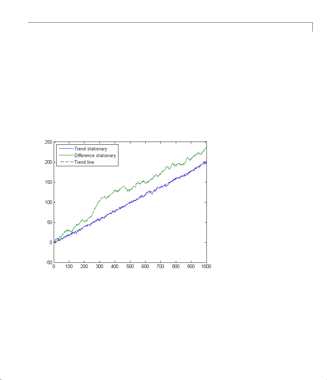
Model Identification

Both processes grow at rate 0.2t. TocalculatethegrowthratefortheTSP, which has a linear term 0.02t,setε

(t)=0. Thensolvethemodely1(t)=a

+ ct for a and c:

a + ct =0.9(a + c(t–1)) + 0.02t.

The solution is a = –1.8, c =0.2.

Aplotfort = 1:1000 shows the TSP stays very close to the trend line, while the D SP has persistent deviations away from the trend line.

Forecasts based on the two series are different. To see this difference, plot the predicted behavior of the two series using the

vgxpred function. The following

plot shows the last 100 data points in the two series and predictions of the next 100 points, including confidence bounds.

3-13

3 Model Selection

3-14

The TSP the DS the tr y =0.2

Spur

in re

Supp as r

has confidence intervals that do not grow with time. Whereas,

P has confidence intervals that grow. Furthermore, the TSP goes to

end line quickly, while the DSP does not tend towards the trend line

t asymptotically.

ious Regression. The presence of unit roots can lead to false inferences

gressions between time series.

ose x

and ytareunitrootprocesseswithindependent increments, such

andom walks with drift

Model Identification

xt= c1+ x y

= c2+ y

where ε

(t) are independent innovations processes. Regressing y on x results,

t–1

+ ε1(t)

+ ε2(t),

in general, in a nonzero regression coefficient, and significant coefficient of determination R

. This result holds d es pite xtand ytbeing independent

random walks.

If both processes have trends (c because of their linear trends. However, even if the c roots in the x

and ytprocesses yields correlation. For more information on

≠ 0), there is a correlation between x and y

= 0, the presence of unit

spurious regression, see Granger and Newbold [28].

Available Tests

There are four Econometrics Toolbox tests for unit roo ts. These functions test for the existence of a single unit root; when there are two or more unit roots, their results might not be valid.

• “Dickey-Full er and Phillips-Perron Tests” on page 3-15

• “KPSS Test” on page 3-16

• “Variance Ratio Test” on page 3-16

Dickey-Fuller and Phillips-Perron Tests.

Dickey-Fuller test.

pptest performs the Phillips-Perron test. These two

classes of tests have a null hypothesis of a unit root process of the form

adftest performs the augmented

= y

+ c + dt + et,

t–1

which the functions test against an alternative model

= ay

+ c + dt + et,

t–1

where a < 1. The null and alternative models for a Dickey-Fuller test are like those for a Phillips-Perron test. The d ifference is

adftest extends the model

with extra parameters accounting for serial correlation among the residues:

= c + dt + ay

t –1

+ b1Δy

t –1

+ b2Δy

+...+ bpΔy

t –2

t – p

+ e(t),

3-15

3 Model Selection

where

• L is the lag operator: Ly

• Δ =1–L,soΔy

= yt– y

t–1

= y

t–1

• e(t) is the innovations process.

Phillips-Perron adjusts the test statistics to account for serial correlation.

There are three variants of both following values of the

•

'AR' assumes c and d, which appear in the preceding equations, are both 0. 'ARD' assumes d is 0.The'ARD' alternative has mean c/(1–a); the 'AR'

•

'model' parameter:

adftest and pptest, corresponding to the

alternative has mean 0.

'TS' makes no assumption about c and d.

•

For informatio n on how to choose the appropriate value of

KPSS Test. The K PSS test,

kpsstest, is an inverse of the Phillips-Perron

'model',see.

test: it reverses the null and alternative hypotheses. The KPSS test uses the model:

= ct+ dt + ut,with

= c

t–1

+ vt.

3-16

Here u variance σ

is a stationary process, and vtis an i.i.d. process with mean 0 and

. The null hypothesis is that σ2= 0, so that the random walk term

becomes a constant intercept. The alternative is σ2> 0, which introduces

the unit root in the random walk.

Variance Ratio Test. Thevarianceratiotest,

vratiotest, is based on

the fact that the variance of a random walk increases linearly with time.

vratiotest can also take into account heteroscedasticity, where the variance

increases at a variable rate with time. The test has a null hypotheses of a random walk:

Δy

= et.

Model Identification

Testing for Unit Roots

• “Transform Data” on page 3-17

• “Choose Models to Test” on page 3-17

• “Determine Appropriate Lags” on page 3-17

• “Run Tests” on page 3-18

Transform Data. Transformyourtimeseriestobeapproximatelylinear

before testing for a unit root. If a series has exponential growth, take its logarithm. For e xample, GDP and consumer prices typically have exponential growth, so test their logarithms for unit roots. There is more discussion of this topic in “Data P reprocessing” on page 8-12.

If you want to transform your data to be stationary instead of approximately linear, unit root tests can help you determine whether to difference your data, or to subtract a linear trend. For a discussion of this topic, see .

Choose Models to Test.

• For

adftest or pptest,choosemodel in as follows:

- If your data shows a linear trend, set model to 'TS'.

- If your data shows no trend, but seem to have a nonzero mean, set

model to 'ARD'.

- If your data shows no trend and seem to have a zero mean, set model

to 'AR' (the default).

• For

Determine Appropriate Lags. Setting appropriate lags depends on the

test you use:

•

kpsstest,settrend to true (default)ifthedatashowsalineartrend.

Otherwise, set

vratiotest,setIID to true if you want to test for independent,

identically distributed innovations (no heteroscedasticity). Otherwise, leave

IID at the default value, false. Linear trends do not affect vratiotest.

adftest —Onemethodistobeginwithamaximumlag,suchasthe

one recommended by Schwert [56]. Then, test down by assessing the

trend to false.

3-17

3 Model Selection

significance of the coefficient of the term at lag p

. Schwert recommends

max

amaximumlagof

where

maximum lag 12 100

max

is the integer part of x. The usual t statistic is appropriate

⎣⎦

⎢

()

⎣

for testing the significance of coefficients, as reported in the

/,==

⎥ ⎦

reg output

structure. Another method is to combine a measure of fit, such as SSR, with

information criteria such as AIC, BIC, and HQC. These statistics also appear in the

reg output structure. Ng and Perron [49] provide further

guidelines.

•

kpsstest — One method is to begin w ith few lags, and then evaluate

the sensitivity of the results by adding more lags. For consistency of the Newey-West estimator, the number of lags must go to infinity as the sample size increases. Kwiatkowski et al. [36] suggest using a number of lags on the order of T

For an example of choosing lags for

pptest — O ne method is to begin with few lags, and then evaluate the

•

1/2

,whereT isthesamplesize.

kpsstest,see.

sensitivity of the results by adding more lags. Another method is to look at sample autocorrelations of y

– y

; slow rates of decay require more lags.

t–1

The Newey-West estimator is consistent if the number of lags is O(T where T is the effective sample size, adjusted for lag and missing values. White and Domowitz [57] and Perron [50] provide further guidelines.

1/4

3-18

For an example of choosing lags for

vratiotest does not use lags.

•

pptest,see.

Run Tests. Run multiple tests simultaneously by entering a vector of parameters for

lags, alpha, model,ortest. All vector parameters must have

the same length. The test expands any scalar parameter to the length of a vector parameter. For an example using this technique, see .

Examples of Unit Root Tests

• “Example: Testing Simulated Data for a Unit Root” on page 3-19

Model Identification

• “Example: Testing Wage Data for a Unit Root” on page 3-23

• “Example: Testing Stock Data for a Random Walk” on page 3-26

Example: Testing Simulated Data for a Unit Root. This example

generates trend-stationary, difference -stationary, stationary (AR(1)), and heteroscedastic random walk time series using simulated data. The example shows how to test the resulting series. It also shows that the tests give the expected results.

1 Generate four time series:

T = 1e3; % Sample size strm = RandStream('mt19937ar','Seed',142857); % reproducible t = (1:T)'; % time multiple

y1 = randn(strm,T,1) + .2*t; % trend stationary y2 = randn(strm,T,1) + .2; y2 = cumsum(y2); % difference stationary y3 = randn(strm,T,1) + .2; for ii = 2:T

y3(ii) = y3(ii) + .99*y3(ii-1); % AR(1) end sigma = (sin(t/200) + 1.5)/2; % std deviation y4 = randn(strm,T,1).*sigma + .2; y4 = cumsum(y4); % heteroscedastic

2 Plot the first 100 points in each series:

y=[y1y2y3y4]; plot1 = plot(y(1:100,:)); set(plot1(1),'LineWidth',2) set(plot1(3),'LineStyle',':','LineWidth',2) set(plot1(4),'LineStyle',':','LineWidth',2) legend('trend stationary','difference stationary','AR(1)',...

'Heteroscedastic','location','northwest')

3-19

3 Model Selection

3-20

It is diff looking

3 Plot the entire data set:

icult to distinguish which series comes from which model simply by at these initial segments of the series.

plot2 = plot(y); set(plot2(1),'LineWidth',2) set(plot2(3),'LineStyle',':','LineWidth',2) set(plot2(4),'LineStyle',':','LineWidth',2) legend('trend stationary','difference stationary','AR(1)',...

'Heteroscedastic','location','northwest')

Model Identification

The diffe

• The tren

• The dif

• The AR(

• The di

4 Per

pur

rences between the series are clearer here:

d stationary series has little deviation from its mean trend.

ference stationary and Heteroscedastic series have persistent

ions away from the trend line.

deviat

1) series exhibits long-run stationary behavior; the others grow

ly.

linear

fference stationary and Heteroscedastic series appear similar. But

e that the Heteroscedastic series has much more local variability

notic

time 300, and much less near time 900. The model variance is

near

mal when sin(t/200) = 1, at time 200*π/2 ≈ 314. The model variance

maxi

nimal when sin(t/200) = –1, at time 200*3*π/2 ≈ 942. So the visual

is mi

ability matches the model.

vari

formthefollowingtests(thenumberoflagsissetto poses):

2 for demonstration

3-21

3 Model Selection

• Test the three growing series:

- Null: y

- Alternative: y

= y

+ c + b1Δy

t –1

= ay

+ b2Δy

t –1

+ c + dt + b1Δy

t –1

t–2

• Test the stationary AR(1) series:

- Null: y

- Alternative: y

= y

t –1

+ b1Δy

= ay

t –1

+ b1Δy

+ b2Δy

t –1

t–2

+ b2Δy

+ e(t)

• Test all the series:

- Null: Var(Δy

- Alternative: Var(Δy

) = constant

) ≠ constant

Test Results

Tested Model

'TS' adftest(y1,

'AR' adftest(y3,

Data Generation Process

Trend stationary y1

'model','ts', 'lags',2)

Difference stationary y2

adftest(y2, 'model','ts', 'lags',2)

Stationary AR(1) y3

'model','ar', 'lags',2)

+ e(t)

t –1

t–2

+ b2Δy

+ e(t)

t–2

Heteroscedastic Random Walk y4

adftest(y4, 'model','ts', 'lags',2)

3-22

Test Results (Continued)

Model Identification

Tested Model

Stationary (KPSS)

Random Walk

Data Generatio

Trend station

ary

kpsstest(y1, 'lags',32, 'trend',true)

vratiotest(y1)

In each

• The fi

• The ne

• The fi

resu to ma

n Process

Difference stationary y2

kpsstest(y2, 'lags',32, 'trend',true)

vratiotest(y2, 'IID',true)

Stationary AR(1) y3

kpsstest(y3, 'lags',32)

vratiotest(y3, 'IID',true)

Heteroscedas Random Walk y

kpsstest(y4, 'lags',32, 'trend',true)

vratiotest(y4)

vratiotest (y4, 'IID',true)

cell of the table:

rst line represents the command.

xt line represents the result of running the command.

nal symbol indicates whether the result matches the expected

lt based on the data generation process:

for a match, × for failure

tch.

tic

• You c

The

vra

is a nu an

ample: Testing Wage Data for a Unit Root. This example tests

hether there is a unit root in wages in the manufacturing sector. The data

or the years 1900–1970 is in the Nelson-Plosser data set [47].

1 Load the Nelson-Plosser data. Extract the nominal wages data:

an substitute

re is one incorrect inference. In the lower right corner of the table,

tiotest

does not reject the hypothesis that the heteroscedastic process

n IID random walk. This inference depends on the pseudorandom

mbers. Run the data generation procedure with

d the inference changes.

pptest for adftest.

Seed equal to 857142

3-23

3 Model Selection

load Data_NelsonPlosser wages=Dataset.WN;

2 Trim the NaN data from the series and the associated dates. (This step is

optional, since the test ignores NaN values.)

wdates = dates(isfinite(wages)); wages = wages(isfinite(wages));

3 Plot the data to look for trends:

plot(wdates,wages) title('Wages')

3-24

4 The plot suggests exponential growth. Use the log of wages to linearize

the data set:

lwages = log(wages); plot(wdates,lwages) title('Log Wages')

Model Identification

5 The data appear to have a linear trend. Test the hypothesis that this

process is a unit root process with a trend (difference stationary), aga in st the alternative that there is no unit root (trend stationary). Following , set

'lags' = [2:4]:

[h,pValue] = pptest(lwages,'lags',[2:4],'model','TS')

000

pValue =

0.6303 0.6008 0.5913

pptest

6 Check the inference using kpsstest. Following , set 'lags' to [7:2:11]:

fails to reject the hypothesis of a unit root at all lags.

[h,pValue] = kpsstest(lwages,'lags',[7:2:11]) Warning: Test statistic #1 below tabulated critical values: maximum p-value = 0.100 reported.

3-25

3 Model Selection

> In kpsstest>getStat at 606

In kpsstest at 290 Warning: Test statistic #2 below tabulated critical values: maximum p-value = 0.100 reported. > In kpsstest>getStat at 606

In kpsstest at 290 Warning: Test statistic #3 below tabulated critical values: maximum p-value = 0.100 reported. > In kpsstest>getStat at 606

In kpsstest at 290

000

pValue =

0.1000 0.1000 0.1000

3-26

kpsstest

If the result would have been

fails to reject the hypothesis that the data is trend-stationary.

[1 1 1], the two inferences would provide

consistent evidence of a unit root. It remains unclear whether the data has a unit root. This is a typical result of tests on many macroeconomic series.

The warning that the test statistic “...is below tabulated critical values” does not indicate a problem.

kpsstest has a limited set of calculated

critical values. When the calculated test statistic is outside this range, the test reports the p-value at the endpoint. So, in this case,

pValue reflects

the closest tabulated value. When a test statistic lies inside the span of tabulated values,

kpsstest reports linearly interpolated values.

Example: Testing Stock Data for a Random Walk. This example uses market data for daily returns of stocks and cash (money market) from the period January 1, 2000 to November 7, 2005. The question is whether a random walk is a good model for the data.

1 Load the data.

load CAPMuniverse

Model Identification

2 Extract two series to test. The first column of data is the daily return of a

technology stock. The last (14th) column is the daily return for cash (the daily money market rate).

tech1 = Data(:,1); money = Data(:,14);

The returns are the logs of the ratios of values at the end of a day over the values at the beginning of the day.

3 Convert the data to prices (values) instead of returns. vratiotest takes

prices as inputs, as opposed to returns.

tech1 = cumsum(tech1); money = cumsum(money);

4 Plotthedatatoseewhethertheyappeartobestationary:

subplot(2,1,1) plot(Dates,tech1); title('Log(relative stock value)') datetick('x') hold('on') subplot(2,1,2); plot(Dates,money) title('Log(accumulated cash)') datetick('x') hold('off')

3-27

3 Model Selection

3-28

Cash has a small variability, and appears to have long-term trends. The stock series has a good deal of variability, and no definite trend, tho ugh it appearstoincreasetowardstheend.

5 Test whether the stock series matches a random walk:

[h,pValue,stat,cValue,ratio] = vratiotest(tech1)

pValue =

0.1646

stat =

-1.3899

cValue =

1.9600

ratio =

0.9436

Model Identification

vratiotest

does not reject the hypothesis that a random walk is a

reasonable model for the stock series.

6 Test whether an i.i.d. random walk is a reasonable model for the stock

series:

[h,pValue,stat,cValue,ratio] = vratiotest(tech1,'IID',true)

pValue =

0.0304

stat =

-2.1642

cValue =

1.9600

ratio =

0.9436

vratiotest

reasonable model for the

vratiotest indicates that the most appropriate model of the tech1 series

rejects the hypothesis that an i.i.d. random walk is a

tech1 stock series at the 5% level. Thus,

is a heteroscedastic random walk.

7 Test whether the cash series matches a random walk:

[h,pValue,stat,cValue,ratio] = vratiotest(money)

pValue =

3-29

3 Model Selection

4.6093e-145

stat =

25.6466

cValue =

1.9600

ratio =

2.0006

vratiotest

reasonable model for the cash series (pValue = 4.6093e-145). Removing a linear trend from the cash series does not affect the resulting statistics.

emphatically rejects the hypothesis that a random walk is a

Misspecification Tests

• “The Classical Misspecification Tests” on page 3-30

• “Covariance Estimators” on page 3-33

• “Example: Specifying Distribution Parameters” on page 3-34

• “Example: Comparing GARCH Models” on page 3-40

• “Testing Multiple Time Series” on page 3-43

The Classical Misspecification Tests

Econometrics Toolbox includes three classical frameworks for model misspecification testing:

• Lagrange multiplier test (

• Likelihood ratio test (

• Wald test (

waldtest)

lmtest)

lratiotest)

3-30

These functions all estimate the difference in maximum loglikelihood between a restricted model and an unrestricted model. They test whether unrestricted model parameters are statistically significant.

Model Identification

Some examples of model restrictions that can be tested in these frameworks are:

• A GARCH(1,1) model (restricted) versus a GARCH(2,1) model (unrestricted, see “Types of GARCH Models” on page 1-14)

• A V ARMA model with two autoregressive lags (restricted) versus a VARMA model w ith three autoregressive lags (unrestricted, see “Types of Multiple Time Series Models” on page 8-2)

• A Gamma(k,θ) distribution with k = 1 (restricted) versus a Gamma(k,θ) distribution with no restrictions on parameters

The setting for all of these tests is a vector of model parameters θ,data d, and a loglikelihood function L(θ|d). When data represent independent observations, L is a sum of individual loglikelihoods over all data points. The

unrestricted optimizer r(θ) = 0 occurs, in general, at some



LdLd



||.

()



maximizes L. The optimizer subject to restrictions





. Therefore,

Each test assesses the difference in loglikelihood in a different way:

•

lratiotest finds the difference of loglikelihoods (the log of the likelihood

and



directly. If the restrictions are insignificant, this

). Since r(



()

∇



,since



) = 0, if the restrictions are



is the

∇

()







ratio) at difference should be near 0.

•

lmtest uses the gradient (score), ∇L(θ).

unrestricted maximum of L. If the restrictions are insignificant, should also be near 0.

waldtest finds the value of r(

•

insignificant, this should also be near 0.

lratiotest evaluates the difference in loglikelihoods directly. lmtest

and waldtest do so indirectly, with the idea that insignificant changes in the evaluated quantities are equivalent to insignificant changes in the parameters. This equivalence depends on the curvature of the loglikelihood surface in the neighborhood of the maximum likelihood estimator. As a result,



3-31

3 Model Selection

Types of Hypothe sis Tests

the Wald and Lagrange multiplier tests include an estimate of parameter covariance in the formulation of the test statistic.

Each test requires different input data. The following table shows the input requirements for the tests, and some MATLAB functions that can provide the inputs.

Test

lratiotest

lmtest

waldtest

Required Inputs

Unrestricted maximum loglikelihood (

uLL)

Helper Functions for the Inputs

garchfit, vgxvarx, Optimization Toolbox fmincon, fminunc, Statistics Toolbox mle, betalike, explike, and other functions

named

*like (see “Negative Log-Likelihood

Functions” in the Statistics Toolbox user guide documentation).

Restricted maximum loglikelihood (

rLL)

garchfit, vgxvarx, Optimization Toolbox fmincon

Degrees of freedo m Number of restrictions Score a t restricted maximum Optimization Toolbox fmincon Estimated unrestricted covariance

You must compute the Jacobian analytically

at restricted maximum Degrees of freedo m Number of restrictions Restriction function r at

unrestricted maximum R =Jacobianofr at unrestricted

maximum

Optimization Toolbox fmincon, fminunc can find the maximum point

Optimization Toolbox fmincon, fminunc can find the maximum point; you must compute the Jacobian analytically

Estimated unrestricted covariance at unrestricted maximum

garchfit, vgxvarx, Statistics Toolbox mlecov

3-32

• Use fmincon or fminunc to find the location and value of restricted or unrestricted maxima of the loglikelihood functions.

fminunc minimize,soinputthenegativeloglikelihood function to obtain

fmincon and

Model Identification

amaximum. (Don’tforgettotakethenegativeoftheresultforthetrue loglikelihood.)

•

garchfit and vgxvarx return both the loglikelihood and an estimated

covariance at the unrestricted maximizer.

• If you have a Symbolic Math Toolbox™ license, you can obtain the score for the Lagrange multiplier test, or the Jacobian for the Wald test, using the

diff or jacobian functions. Using jacobian twice yields a Hessian

matrix, which y ou can use to calculate the co variance. See “Example: Using Symbolic Math Toolbox Functions to Calculate Gradients and Hessians” in the O ptimization Toolbox User’s Manual for an example.

Covariance Estimators

lmtest and waldtest require an estimate of the parameter covariance.

Parameter covariance is related to the curvature of the loglikelihood function. This curvature indirectly indicates parameter significance used by the two tests.

There are several common methods for estimating the parameter covariance, including:

• Outer Product of Gradients (OPG). Let G be the matrix of contributions to the gradient, the gradient of the loglikelihood function L.(Thisisalso called the CG matrix.) G is an ndata-by-n matrix,witheachrowbeing the score at one data point. ndata is the number of data points, and n is the num ber of dimensions in the gradient. Then (G

–1

'G)

is an estimate of the covariance, an n-by-n m atrix. This estimator is convenient because it requires only first derivatives.

• Inverse negative Hessian. The covariance estimator is:

cov( , )

⎛

 −

⎜ ⎜ ⎝

∂



∂∂

⎞



()

⎟ ⎟

⎠

−21

.ij

There are two forms of this estimator.

- Observed Hessians. Calculate the Hessian of the loglikelihood. Take the

inverse of the negative of this quantity.

3-33

3 Model Selection

- Expe cted Hessian. Calculate the expected value of the H essian of the

loglikelihood. Take the inverse of the negative of this quantity. This requires calculating analytic expectations, so obtaining this es timate is usually m ore difficult than the observed Hessian.



For

lmtest, evaluate the estimator at the restricted maximum point

waldtest, evaluate the estimator at the unrestricted maximum point

garchfit and vgxvarx return an estim ated covariance matrix, along with

other parameter estimates. and

vgxvarx returns an estimator based on the expected Hessian.

garchfit returns an estimator based on OPG,

Example: Specifying Distribution Parameters

The following reproduces the example in Greene [29], Sec. 16.6.4. The example fits a Gamma distribution to the simulated education and income data in

IncomeData.mat:

load Data_Income1 x = Dataset.EDU; y = Dataset.INC;



.For



3-34

The unrestricted model has a likelihood l given by the probability density function for the Gamma distribution:





ly x y e

(|,, )



()





−



−

where



x=+

This yields the loglikelihood

Model Identification

Ll yy

( , ) log ( , ) log log ( ) ( ) log( ) .

      

==−+−−Γ 1

(3-1)

Gamma distributions are sums of ρ exponential distributions, so admit natural restrictions on the value of ρ. Greene’s restricted m odel is ρ =1,a simple exponential distribution.

lratiotest. To perform this test, you need estimates of both the unrestricted and restricted maximum likelihood. To find the unrestricted maximum likelihood estimates of β and ρ,youcanuse

% Negative loglikelihood function with parameters p = [beta,rho]: nLLF = @(p)sum(p(2)*(log(p(1) + x)) + gammaln(p(2))...

-(p(2) - 1)*log(y) + y./(p(1) + x));

options = optimset('LargeScale','off'); % 'on' with gradients % Unrestricted estimate: General gamma model [umle,unLL] = fminunc(nLLF,[.1 .1],options)

fminunc:

This code produces:

umle =

-4.7186 3.1509

unLL =

82.9160

To find the unrestricted maximum likelihood estimates:

ubeta = umle(1); % Unrestricted beta estimate urho = umle(2); % Unrestricted rho estimate uLL = -unLL; % Unrestricted loglikelihood

lratiotest

% Restricted estimate with rho = p(2) = 1 rnLLF = @(p)nLLF([p 1]); [rmle,rnLL] = fminunc(rnLLF,.1,options)

rmle =

also requires the restricted maximum likelihood:

15.6027

3-35

3 Model Selection

rnLL =

88.4363

rbeta = rmle(1); % Restricted beta estimate rrho = 1; % Restricted rho rLL = -rnLL; % Restricted loglikelihood

To evaluate the likelihood ratio, be careful to use the negative of unLL and

rnLL. There is one restriction, so dof = 1:

dof = 1; [LRh,LRp,LRstat,cV] = lratiotest(uLL,rLL,dof)

LRh =

LRp =

8.9146e-004

3-36

LRstat =

11.0404

cV =

3.8415

LRh = 1

means lratiotest rejects the restricted hypothesis. This is a strong

rejection: the p-value is less than 1/1000.

lmtest.

lmtest requires the score, and an estimate of the covariance matrix,

evaluated at the restricted parameter estimates.

By analytic calculation, the gradient of the loglikelihood function has components:

∂

 

=− +

∑∑



∂ ∂

=−+

∑∑



∂

iii



log ( ) log .Ψ

Model Identification

Here Ψ(ρ) is the digamma (psi) function, the derivative of the logarithm of Γ(ρ), and n is the number of terms in the sum, which is the number of data points.

The OPG estimator of the covariance is (G

–1

'G)

,whereG is the matrix of gradients. For more information, see . Since the score is evaluated as the sum of these derivatives, the simplest way to estimate the covariance for

lmtest

is to use the OPG estimator.

Calculate the gradient of L at the restricted maximum β =

rbeta, ρ =1,and

calculate the OPG estimator, as follows:

RCG = [-rrho./(rbeta+x)+y.*(rbeta+x).^(-2),...

-log(rbeta+x)-psi(rrho)+log(y)]; Rscore = sum(RCG)'; REstCov1 = inv(RCG'*RCG);

There is one restriction, so dof = 1.

[LMh,LMp,LMstat,LMcv] = lmtest(Rscore,REstCov1,dof)

LMh =

LMp =

7.4744e-005

LMstat =

15.6868

LMcv =

3.8415

LMh = 1

means lmtest rejects the restricted hypothesis. This is a strong

rejection: the p-value is less than 1/10000.

waldtest.

waldtest requires the value and gradient of the restriction

function at the unrestricted maximum. The restriction function is r(β, ρ)=ρ – 1 = 0. This has gradient [0 1]. In other words, at the unrestricted

maximum

=(β, ρ),



3-37

3 Model Selection

r = 3.1509 – 1 R=[01].

R = [0 1];r = urho - 1;n = size(x,1);

TheWaldtestalsorequiresanestimated covariance. This time, use the sum of observed Hessians,

⎡

∂

⎢



∂

⎢

∂

⎢ ⎢



∂∂

⎣

∂



∂∂

∂



∂

⎤ ⎥ ⎥

⎥ ⎥ ⎥

⎦

which you find through analytic calculation:

∂



∂

∂∂



∂ ∂



 

=−

∑∑

=−



∑

=−

Ψ’()..

The e stimated covariance is given by –H

2Ly



–1

, where H is the observed Hessian;

see . Calculate the Hessian and covariance matrices as follows:

UDPsi = psi(1,urho); UH = [sum(urho./(ubeta+x).^2)-2*sum(y./(ubeta+x).^3),...

-sum(1./(ubeta+x)); -sum(1./(ubeta+x)),-n*UDPsi]; UEstCov2 = -inv(UH);

(3-2)

3-38

The Wald test is

[Wh,Wp,Wstat,Wcv] = waldtest(r,R,UEstCov2)

Wh =

Mathworks ECONOMETRICS TOOLBOX 1 user guide

Specifications and Main Features

Frequently Asked Questions

User Manual

Getting Started

Product Overview

Technical Conventions

Time Series Arrays

Conditional vs. Unconditional Variance

Prices, Returns, and Compounding

Stationary and Nonstationary Time Series

Time Series Modeling

Characteristics of Time Series

Forecasting Time Series

Serial Dependence in Innovations

Conditional Mean and Variance Models

Conditional Mean Models

Conditional Variance Models

GARCH Models

Introduction

Modeling with GARCH

Limitations of GARCH Models

Types of GARCH Models

Comparing GARCH Models

The Default Model

Example: Using the Default Model

Loading the Price Series Data

Converting the Prices to a Return Series

Checking for Correlation in the Return Series

Checking for Correlation in the Squared Returns

Quantifying the Correlation

Comparing Correlation of the Standardized Innovations

Example Workflow

Estimation

Forecasting

Simulation

Analysis

Model Selection

Specification Structures

About Specification Structures

Specification Structure Parameter Names

Conditional Mean Model

Conditional Variance Models

Working with Specification Structures

Creating Specification Structures

Modifying Specification Structures

Retrieving Specification Structure Values

Example: Specification Structures

Model Identification

Autocorrelation and Partial Autocorrelation

Unit Root Tests

What Is a Unit Root Test?

Modeling Unit Root Processes

Available Tests

Testing for Unit Roots

Examples of Unit Root Tests

Test Results

Misspecification Tests

The Classical Misspecification Tests

Types of Hypothe sis Tests

Covariance Estimators

Example: Specifying Distribution Parameters