

Page 1

Curve Fitting Tool
User’s Guide
box™ 2
Page 2

How to Contact The MathWorks
www.mathworks.
comp.soft-sys.matlab Newsgroup
www.mathworks.com/contact_TS.html Technical Support
suggest@mathworks.com Product enhancement suggestions
bugs@mathwo
doc@mathworks.com Documentation error reports
service@mathworks.com Order status, license renewals, passcodes
info@mathwo
com
rks.com
rks.com
Web
Bug reports
Sales, prici
ng, and general information
508-647-7000 (Phone)
508-647-7001 (Fax)
The MathWorks, Inc.
3 Apple Hill Drive
Natick, MA 01760-2098
For contact information about worldwide offices, see the MathWorks Web site.
Curve Fitting Toolbox™ User’s Guide
© COPYRIGHT 2001–20 10 by The MathWorks, Inc.
The software described in this document is furnished under a license agreem ent. The softwar e may be used
or copied only under the terms of the license agreement. No part of this manual may be photocopied or
reproduced in any form without prior written consent from The MathW orks, Inc.
FEDERAL ACQUISITION: This provision applies to all acquisitions of the Program and Documentation
by, for, or through the federal government of the United States. By accepting delivery of the Program
or Documentation, the government hereby agrees that this software or documentation qualifies as
commercial computer software or commercial computer software documentation as such terms are used
or defined in FAR 12.212, DFARS Part 227.72, and DFARS 252.227-7014. Accordingly, the terms and
conditions of this Agreement and only those rights specified in this Agreement, shall pertain to and govern
theuse,modification,reproduction,release,performance,display,anddisclosureoftheProgramand
Documentation by the federal government (or other entity acquiring for or through the fede ra l government)
and shall supersede any conflicting contractual terms or conditions. If this License fails to meet the
government’s needs or is inconsistent in any respect with federal procurement law, the government agrees
to return the Program and Docu mentation, unused, to The MathWorks, Inc.
Trademarks
MATLAB and Simulink are registered trademarks of The MathWorks, Inc. S ee
www.mathworks.com/trademarks for a list of additional trademarks. Other product or brand
names may be trademarks or registered trademarks of their respective holders.
Patents
The MathWorks products are protected by one or more U.S. patents. Please see
www.mathworks.com/patents for more information.
Page 3

Revision History
July 2001 First printing New for V ersion 1 (Release 12.1)
July 2002 Second printing Revised for Version 1.1 (Release 13)
June 2004 Online only Revised for Version 1.1.1 (Release 14)
October 2004 Online only Revised for Version 1.1.2 (Release 14SP1)
March 2005 Online only Revised for Version 1.1.3 (Release 14SP2)
June 2005 Third printing Minor revision
September 2005 Online only Revised for Version 1.1.4 (Release 14SP3)
March 2006 Online only Revised for Version 1.1.5 (Release 2006a)
September 2006 Online only Revised for Version 1.1.6 (Release 2006b)
November 2006 Fourth printing Minor revision
March 2007 Online only Revised for Version 1.1.7 (Release 2007a)
September 2007 Online only Revised for Version 1.2 (Release 2007b)
March 2008 Online only Revised for Version 1.2.1 (Release 2008a)
October 2008 Online only Revised for Version 1.2.2 (Release 2008b)
March 2009 Online only Revised for Version 2.0 (Release 2009a)
September 2009 Online only Revised for Version 2.1 (Release 2009b)
March 2010 Online only Revised for Version 2.2 (Release 2010a)
Page 4

Page 5

Getting Started
1
Product Overview ................................. 1-2
Major Features
Interactive and Programmatic Environments
................................... 1-2
........... 1-2
Contents
Curve Fitting
Interactive Curve Fitting
Programmatic Curve Fitting
Surface Fitting
Interactive Surface Fitting
Programmatic Surface Fitting
...................................... 1-4
........................... 1-4
........................ 1-4
.................................... 1-5
.......................... 1-5
....................... 1-5
Interactive Curve Fitting
2
Interactive C urve Fitting Example .................. 2-2
Opening Curve Fitting Tool
Importing Data
Interactive Curve Fitting Procedure
Analyzing the Fit
Saving Your Work
Preprocessing Data
Importing Data
Viewing Data
Smoothing Data
Excluding and Sectioning Data
Missing Values and Outliers
................................... 2-3
.................................. 2-16
................................. 2-19
................................ 2-22
................................... 2-22
..................................... 2-26
................................... 2-29
......................... 2-2
.................. 2-5
...................... 2-37
........................ 2-47
Fitting Data
....................................... 2-48
v
Page 6

Parametric Fitting ................................. 2-52
Introduction
Library M odels
Specifying Fit Options
Example: Rational Fit
Example: Robust Fitting
...................................... 2-52
................................... 2-53
............................. 2-58
............................. 2-62
........................... 2-68
Creating Custom Models
Custom Models vs. Library Models
Creating Custom Models
Editing and Saving Custom Models
Example: Legendre Polynomial
Example: Fourier Series
Example: Gaussian with Exponential Background
Nonparametric Fitting
Introduction
Example: Nonparametric Fitting
...................................... 2-106
........................... 2-77
................... 2-77
........................... 2-77
................... 2-81
...................... 2-83
............................ 2-91
...... 2-101
............................. 2-106
..................... 2-106
Interactive Surface Fitting
3
Fitting a Surface .................................. 3-2
Introducing the Surface Fitting Tool
How to Fit a Surface
Opening the Surface Fitting Tool
Selecting Data
Refining Your Fit
Removing Outliers
Selecting Validation Data
Exploring and Customizing Plots
............................... 3-3
.................................... 3-4
................................. 3-6
................................ 3-7
........................... 3-8
.................. 3-2
..................... 3-4
..................... 3-8
vi Contents
Interactive Su rface Fitting Examples
Franke Data Interactive Surface Fitting Example
Biopharmaceutical Interactive Surface Fitting Example
Selecting Fit Settings
Introduction
Selecting Fit Category
...................................... 3-29
.............................. 3-29
............................. 3-29
................ 3-11
....... 3-11
.. 3-21
Page 7

Using Center and Scale Setting ...................... 3-30
Using Interpolant Fit Category
Using Polynomial Fit Category
Using Lowess Fit Category
Using Custom Equation Fit Category
...................... 3-30
...................... 3-31
.......................... 3-33
................. 3-34
Fitting Mu ltiple Surfaces
Introduction
Fitting Additional Surfaces
Duplicating a Surface Fit
Deleting a Surface Fit
Comparing Surface Fits
Introduction
Displaying Multiple Fits Simultaneously
Displaying Surface, Residual, and Contour Plots
Using the Statistics in the Table of Fits
Generating C ode and Exporting Fits to the
Workspace
Introducing Programmatic Surface Fitting
Generating Code from the Surface Fitting Tool
Exporting a Fit to the Workspace
Working with Sessions
Overview
Saving Sessions
Reloading Sessions
Removing Se ssio ns
...................................... 3-36
...................................... 3-38
...................................... 3-44
........................................ 3-49
................................... 3-49
................................ 3-49
................................ 3-49
.......................... 3-36
......................... 3-36
........................... 3-37
.............................. 3-37
............................ 3-38
.............. 3-38
............... 3-42
............. 3-44
.................... 3-46
............................. 3-49
........ 3-40
......... 3-44
Programmatic Curve and Surface Fitting
4
Introducing Programmatic Curve Fitting ............ 4-2
Using Curve Fitting Objects and Methods
Interactive Code Generation
Curve Fitting Objects and Methods
........................ 4-5
............. 4-2
................. 4-9
vii
Page 8

Overview ........................................ 4-9
Curve Fitting Objects
Curve F itting Methods
Workflow for Object-Oriented Fitting
Examples
........................................ 4-15
.............................. 4-10
............................. 4-11
................. 4-13
Generating Code From Curve Fitting Tool
Overview
The Generated Code
Running the Generated File
Components of the Generated File
Modifying the Code
Programmatic Surface Fitting
Surface Fitting Objects and Methods
Automotive Fuel Efficiency Programmatic Surface Fitting
Example
Biopharmaceutical Drug Interaction Programmatic Surface
Fitting Example
........................................ 4-30
............................... 4-31
......................... 4-33
.................... 4-35
................................ 4-38
...................... 4-41
.................. 4-41
....................................... 4-42
................................ 4-53
........... 4-30
Curve Fitting Techniques
5
Data Tran sformations .............................. 5-2
Filtering and Smoothing
Moving Average Filtering
Savitzky-Golay Filtering
Local Regression Smoothing
Smoothing Splines
................................. 5-13
........................... 5-4
........................... 5-4
............................ 5-6
......................... 5-7
viii Contents
Least-Squares Fitting
Introduction
Error Distributions
Linear Least Squares
Weighted Least Squares
Robust Least Squares
Nonlinear Least Squares
...................................... 5-16
.............................. 5-16
................................ 5-17
.............................. 5-18
............................ 5-21
.............................. 5-23
........................... 5-25
Page 9

Residual Analysis .................................. 5-28
Introduction
Computing Residuals
Goodness-of-Fit Statistics
Confidence and Prediction Bounds
Example: Residual Analysis
...................................... 5-28
.............................. 5-29
........................... 5-31
................... 5-34
......................... 5-39
Interpolants
....................................... 5-45
Function Reference
6
Data Preprocessing ................................ 6-2
Data Fittin g
Fit Type Methods
Curve Fit Methods
Surface Fit Methods
Fit P ostprocessing
Information and Help
....................................... 6-2
.................................. 6-2
................................. 6-3
............................... 6-5
................................. 6-6
.............................. 6-7
ix
Page 10

7
A
Functions — Alphabetical List
Bibliography
Index
x Contents
Page 11

Getting Started
• “Product Overview” on page 1-2
• “Curve Fitting” on page 1-4
• “Surface Fitting” on page 1-5
1
Page 12

1 Getting Started
Product Overview
Major Features
Curve Fitting Toolbox™ software is a collection of graphical user interfaces
(GUIs) and functions for curve and surface fitting that operate in the
MATLAB
MATLAB features with:
• Data preprocessing capabilities, such as sectioning, excluding data, and
• Data fitting using parametric and nonparametric models:
In this section...
“Major Features” on page 1-2
“Interactive and Programmatic Environments” on page 1-2
®
technical computing environment. The toolbox supplements
smoothing
- The toolbox includes a library of parametric models, with polynomials,
exponentials, rationals, sums of Gaussians, Fourier polynomials, and
many others.
1-2
- You can also define custom models to precisely reflect the goals of your
data analysis.
- Nonparametric models are available through a variety of smoothers
and interpolants.
• Fitting methods for linear least squares, nonlinear least squares, weighted
least squares, constrained least squares, and robust fitting are available
• Data and fit statistics to assist you in analyzing your models
• Postprocessing capabilities that allow you to interpolate, extrapolate,
differentiate, and integrate the fit
• The ability to save your work in various formats, including workspace
variables, binary files, and automatically generated MATLAB code
Interactive and Programmatic Environments
Curve Fitting Toolbox software allows you to work in two different
environments:
Page 13

Product Overview
• An interactive environment, with Surface Fitting Tool and Curve Fitting
Tool graphical u ser interfaces
• A programmatic environment that allows you to write object-oriented
MATLAB code using curve and surface fitting methods
To open Curve Fitting Tool, type
cftool
To open Surface Fitting Tool, type
sftool
To list the Curve Fitting Toolbox functions for use in MATLAB programming,
type
help curvefit
The code for any function can be opened in the MATLAB Editor by typing
edit function_name
Brief, command lin e help for any function is available by typing
help function_name
Complete documentation for any function is available by t yp ing
doc function_name
You can change the way any toolbox function works by copying and renaming
its file, examining your copy in the editor, and then modifying it.
You can also extend the toolbox by adding your own files, or by using your
code in combination with functio ns from other toolboxes, such a s Statistics
Toolbox™ or Op timization Toolbox™ software.
1-3
Page 14

1 Getting Started
Curve Fitting
Interactive Curve Fitting
To interactively fit curves, see the following sections:
1 “Interactive Curve Fitting Example” on page 2-2
2 “Preprocessing Data” on page 2-22
3
Programmat
To programm
and Surfac
1 “Introduc
2 “Curve Fitting Objects and Methods” on page 4-9
3 “Generating Code From Curve Fitting Tool” on page 4-30
eFitting:
ing Programmatic Curve Fitting” on page 4-2
ic Curve Fitting
atically fit curves, see these sections in Programmatic Curve
1-4
Page 15

Surface Fitting
Interactive Surface Fitting
To interactively fit surfaces, see Chapter 3, “Interactive S urface Fitting” for
information on the following topics:
1 Fitting a surface
2 Selecting fit settings
3 Fitting multiple surfaces
4 Comparing surface fits
5 Generating code files and exporting fits to the workspace
6 “Interactive Surface Fitting Examples” on page 3-11
Programmatic Surface Fitting
To programmatically fit surfaces, see the following topics:
Surface Fitting
1 “Introducing Programmatic Surface Fitting” on page 3-44
2 “Surface Fitting Objects and Methods” on page 4-41
1-5
Page 16

1 Getting Started
1-6
Page 17

Interactive Curve Fitting
• “Interactive Curve Fitting Example” on page 2-2
• “Preprocessing Data” on page 2-22
• “Fitting Data” on page 2-48
• “Parametric Fitting” on page 2-52
• “Creating Custom M odels ” on page 2-77
• “Nonparametric Fitting” on page 2-106
2
Page 18

2 Interactive Curve Fitting
Interactive Curve Fitting Example
In this section...
“Opening Curve Fitting Tool” on page 2-2
“Importing Data” on page 2-3
“Interactive Curve Fitting Procedure” on page 2-5
“Analyzing the Fit” on page 2-16
“Saving Your W ork” on page 2-19
Opening Cur ve Fitting Tool
The C u rve Fitting Tool is a graphical user interface (GU I) that allows you to
• Visually explore one or more data sets and fits as scatter plots.
• Graphically evaluate the goodness of fit using residuals and prediction
bounds.
2-2
• Access additional interfaces for
- Importing, viewing, and smoothing data.
- Fitting data, and comparing fits and data sets.
- Markingdatapointstobeexcludedfromafit.
- Selecting which fits and data sets are displayed in the tool.
- Interpolating, extrapolating, differentiating, or integrating fits.
Open Curve Fitting Tool with the
cftool
cftool command.
Page 19

Interactive Curve Fitting Example
Importing Data
Before you can import data into Curve Fitting Tool, the data variables must
exist in the MATLAB workspace. For this example, the data is stored in the
MATLAB file
load census
The workspace now contains two new variables, cdate and pop:
•
cdate is a column vector containing the years 1790 to 1990 in 10-year
increments.
•
pop is a column vector with the US population figures that correspond
to the years in
You can import data into Curve Fitting Tool with the Data GUI.
census.mat.
cdate.
2-3
Page 20

2 Interactive Curve Fitting
Open the Data GUI by clicking the Data buttononCurveFittingTool. As
shown below, the Data GUI consists of two panes: Data Sets and Smooth. The
Data Sets pane allows you to
• Import predictor (
import we ights, then they are assumedtobe1foralldatapoints.
• Specify the name of the data set.
• Preview the data.
To load
1 Select the variable names cdate and pop from the XDataand YDatalists.
cdate and pop into Curve Fitting Tool,
The data is displayed in the Preview window.
X) data, response (Y) data, and weights. If you do not
2-4
The Smooth pane is described in “Preprocessing D ata” on page 2-22.
ick the Create data set button to complete the data import process.
2 Cl
Page 21

Interactive Curve Fitting Example
3 Click Close.
Interactive Curve Fitting Procedure
You fit data with the Fitting GU I.
Open the Fitting GUI by clicking the Fitting buttononCurveFittingTool.
The F itting GUI consists of tw o parts: the Fit Editor and the Table of Fits.
The Fit Editor allows you to
• Specify the fit nam e, the current data set, and the exclusion rule.
• Explore various fits to the current data set u sing a library or custom
equation, a smoothing spline, or an interpolant.
• Override the default fit options such as the coefficient sta r tin g values.
• Compare fit results including the fitted coefficients and goodness of fit
statistics.
The Table of Fits allows you to
• Keep track of all the fits and their data sets for the current session.
• Display a summary of the fit results.
• Save or delete the fit results.
The Data Fitting Procedure
For this example, begin by fitting thecensusdatawithaseconddegree
polynomial. Then continue fitting the data using polynomial equations up to
sixth degree, and a single-term exponential equation.
Thedatafittingprocedurefollowsthesesteps:
1 From the Fit Editor,clickNew Fit.
The new fit always defaults to a linear polynomial fit type. Use New Fit
at the beginning of your curve fitting session, and when you are exploring
different fit types for a given data set.
2-5
Page 22

2 Interactive Curve Fitting
2 To use a second degree polynomial for the initial fit, select quadratic
polynomial from the Polynomial list. Edit t h e Fit name to
3 Click the Apply button or select the Immediate apply check box. The
library model, fitted coefficients, and goodness of fit statistics are displayed
in the Results area of the Fitting GUI..
The Fitting GUI is shown below with the results of fitting the census data
with a quadratic polynomial.
poly2.
2-6
Page 23

Interactive Curve Fitting Example
Your new fit is plotted in Curve Fitting Tool.
The data, first fit, and residuals in Curve Fitting Tool are shown
below. Display the residuals as a line plot by selecting the menu item
View>Residuals>Lineplot.
2-7
Page 24

2 Interactive Curve Fitting
These residuals indicate that
a better fit may be possible.
2-8
The residuals indicate that a better f it may be possible. Therefore, you
should continue fitting the census data following the procedure outlined in
the beginning of this section.
1 Return to the Fitting GUI.
2 Add new fits to try the other library equations. For fits of a given type (for
example, polynomials), use Copy Fit instead of New Fit because copying
a fit retains the current fit type state thereby requiring fewer steps than
creating a new fit each time. Add polynomial fits up to the sixth degree,
and add an exponential fit.
3 For each new fit look at the R esults pane information, and the residuals
plot in Curve Fitting Tool.
Page 25

Interactive Curve Fitting Example
The residuals from a goo d fit should lo ok random with no apparent pattern.
A pattern, such as a tendency for consecutive residuals to have the same
sign, can be an indication that a better model exists.
4 When you fit higher degree polynomials, the Results area displays this
warning:
Equation is badly conditioned. Remove repeated data points
or try centering and scaling.
When you see this w a rning, to normalize data, in the Fitting GUI select the
Center and scale X data check box.
The warning about scaling arises because the fitting procedure uses the
cdate
values as th e basis for a matrix with very large values. The spread of th e
cdate values results in scaling problems. To address this problem, you can
normalize the
cdate data. Normalization is a process of scaling the predictor
data to improve the accuracy of the subsequent numeric computations. A way
to normaliz e
cdate is to center it at zero mean and scale it to unit standard
deviation. The programmatic equivalent code is:
(cdate - mean(cdate))./st d(cdate)
Note Because the predictor data changes after normalizing, the values of the
fitted coefficients also change when compared to the original data. However,
the functional form of the data and the resulting goodness of fit statistics do
not change. Additionally, the data is displayed in Curve Fitting Tool using
the original scale.
Determining the Best Fit
To determine the best fit, you should examine both the graphical and
numerical fit results.
Examining the Graphical Fit Results. Your initial approach in determining
the best fit should be to examine the graphs of the fits and residuals. The
graphical fit results shown below indicate that
2-9
Page 26

2 Interactive Curve Fitting
• The fits and residuals for the polynomial equations are all similar, making
it difficult to choose the best one.
• The fit and residuals for the single-term exponential equation indicate it is
a p oor fit overall. Therefore, it is a poor choice for extrapolation.
2-10
Page 27

Interactive Curve Fitting Example
Click Plotting to open the Plotting GUI and remove exp1 from the scatter
plot display.
Because the goal of fitting the census data is to extrapolate the best fit to
predict future population values, you should explore the behavior of the fits
up to the year 2050. You can change theaxeslimitsofCurveFittingToolby
selecting the menu item Tools > Axis Limit Control.
Alter the X Upper Limit to
2050, and increase the Y Upper Limit to 400.The
census data and fits are shown below for an upper abscissa limit of 2050. The
behavior of the sixth degree polynomial fit beyond the data range makes it a
poor choice for extrapolation.
2-11
Page 28

2 Interactive Curve Fitting
2-12
As you can see, you should exercise caution when extrapolating with
polynomial fits because they can diverge wildly outside the data range.
Examining the Numerical Fit Results. Because you can no longer
eliminate fits by examining them graphically, you should examine the
numerical fit results. There are two types of numerical fit results displayed
in the Fitting GUI: goodness of fit statistics and confidence intervals on the
fitted coe fficients. The goodness of fit statistics help y ou determine how well
the curve fits the data. The confidence intervals on the coefficients determine
their accuracy.
Some goodness of fit statistics are displayed in the Results area of the Fit
Editor for a single fit. All goodness of fit statistics are displayed in the Table
of Fits for all fits, which allows for easy comparison.
In this example, the sum of squares due to error (SSE) and the adjusted
R-square statistics are used to help determine the best fit. The SSE statistic
Page 29
Interactive Curve Fitting Example
is the least-squares error o f the fit, with a value closer to zero indicating a
better fit. T he adjusted R-square statistic is generally the best indicator of the
fit quality when you add additional coefficients to your model.
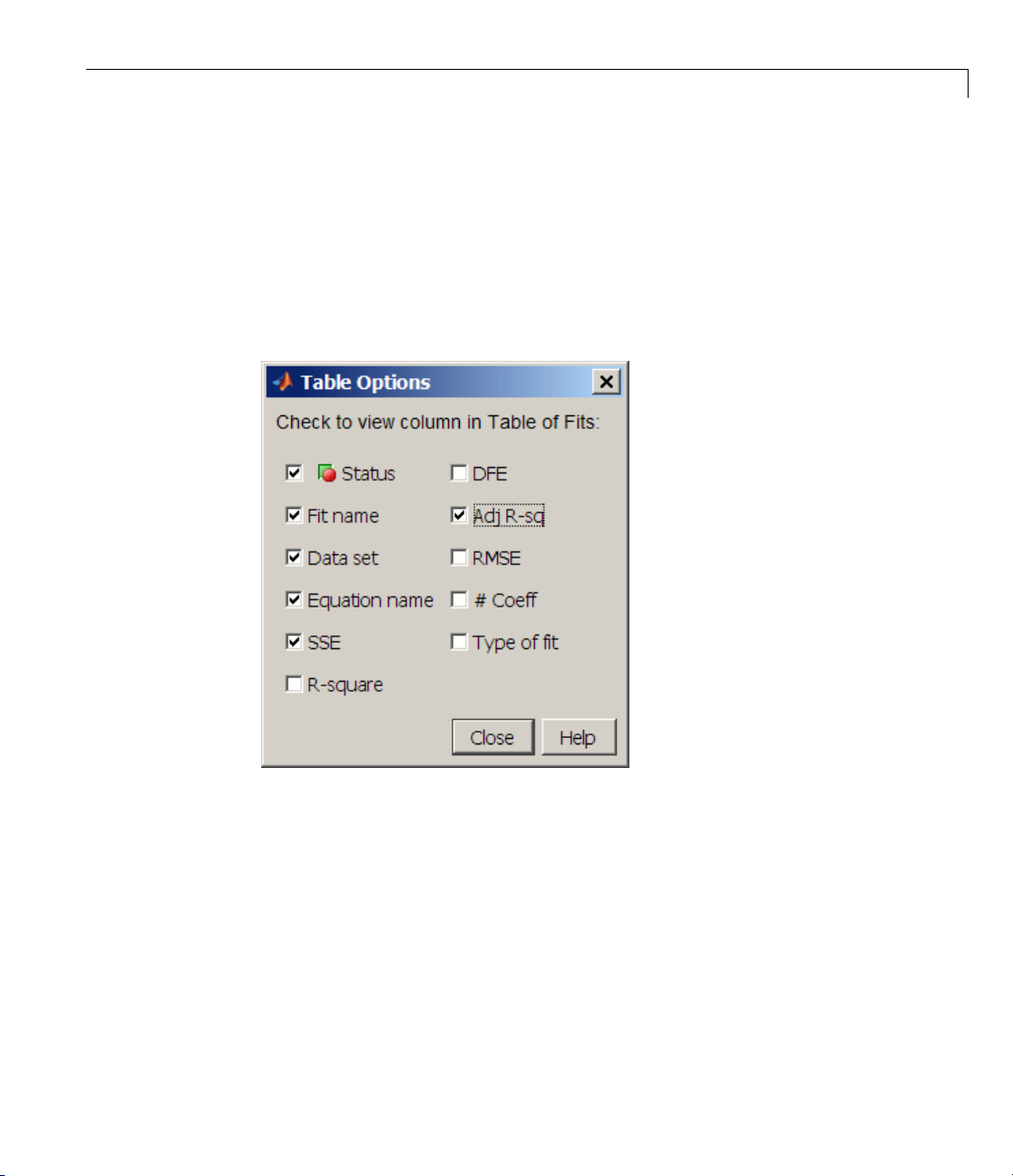
You can modify the information displayed in the Table of Fits with the Table
Options GUI. You open this GUI by clicking the Table options button on
the F itting GUI. As shown below, select the adjusted R-square statistic and
clear the R-square statistic.
The nu
colum
The S
exam
poly
poo
fif
the
al
merical fit results are shown below. You can click the Table of Fits
n headings to sort by statistics results.
SE for
exp1 indicates it is a poor fit, which was already determined by
ining the fit and residuals. The lowest SSE value is associated with
6
. However, the behavior of this fit beyond the data range makes it a
r cho ice for extrapolation. The n ext best SSE value is associated with the
th de gree polynomial fit,
poly5, sugge sting it m ay be the best fit. However,
SSE and adjusted R-square values for the remaining polynomial fits are
l v ery close to each other. Which one should you choose?
2-13
Page 30

2 Interactive Curve Fitting
2-14
To resolve this issue, examine the confidence bounds for the remaining fits
in the Results pane. By default, 95% confidence bounds are calculated. You
can change this level by selecting the menu item View > Confidence Level
from Curve Fitting Tool.
Page 31

Interactive Curve Fitting Example
The p1, p2,andp3 coefficients for the fifth degree polynomial suggest that it
overfitsthecensusdata. However,theconfidenceboundsforthequadratic
fit,
poly2, indicate that the fitted coefficients are known fairly accurately.
Therefore, after examining both the graphical and numerical fit results, it
appears that you should use
poly2 to extrapolate the census data.
Note The fitted coefficients associated with the constant, linear, and
quadratic terms are nearly identical for each polynomial equation. However,
as the polynomial degree increases, the coefficient bounds associated with the
higher degree terms increase, which suggests overfitting.
Saving the Fit Results
By clicking the Save to workspace button, you can save the selected fit and
the associated fit results to the MATLAB workspace. The fit is saved as a
MATLAB object and the associated fit results are saved as structures. This
example saves all the fit results for the best fit,
poly2.
fittedmodel1 is saved as a Curve F itting Toolbox cfit object.
whos fittedmodel1
Name Size Bytes Class
fittedmodel1 1x1 6178 cfit object
Grand total is 386 elements using 6178 bytes
The c fit object display includes the model, the fitted coefficients, and the
confidence bounds for the fitted coefficients.
2-15
Page 32

2 Interactive Curve Fitting
fittedmodel1
fittedmodel1 =
Linear model Poly2:
fittedmodel1(x) = p1*x^2 + p2*x + p3
Coefficients (with 95% confidence bounds):
p1 = 0.006541 (0.006124, 0.00695 8)
p2 = -23.51 (-25.09, -21.93)
p3 = 2.113e+004 (1.964e+004, 2.262e+004)
The goodnes s1 structure contains goodness of fit results.
goodness1
goodness1 =
sse: 159.0293
rsquare: 0.9987
dfe: 18
adjrsquare: 0.9986
rmse: 2.9724
2-16
The output1 structure contains additional information associated with the fit.
output1
output1 =
numobs: 21
numparam: 3
residuals: [21x1 double]
Jacobian: [21x3 double]
exitflag: 1
algorithm: 'QR factorizat ion and solve'
Analyzing the Fit
You can evaluate (interpolate or extrapolate), diffe rentiate, or integrate a fit
over a specified data range with the Analysis GUI. You open this GUI by
clicking the Analysis button on Curve Fitting Tool.
Page 33

Interactive Curve Fitting Example
For this example, you will extrapolate the quadratic polynomial fit to predict
the US population from the year 2000 to the year 2050 in 10 year increments,
and then plot both the analysis results and the data. To do this:
• Enter the appropriate MATLAB vector in the Analyze at Xi field.
• Select the EvaluatefitatXicheck box.
• Select the Plot results and Plot data set check boxes.
• Click the Apply button.
The numerical extrapolation results are shown below.
The extrapolated values and the census data set are displayed tog ether in
a new figure window.
2-17
Page 34

2 Interactive Curve Fitting
2-18
Saving the Analysis Results
By clicking the Save to workspace button, you can save the extrapolated
values as a structure to the MATLAB workspace.
esulting structure is shown below.
The r
analysisresults1
analysisresults1 =
xi: [6x1 double]
yfit: [6x1 double]
Page 35

Saving Your Work
Curve Fitting To
your work. You ca
variables to th
for documentat
In addition to
olbox software provides you with several options for saving
n save one or more fits and the associated fit results as
e MATLAB workspace. You can then use this saved information
ion purposes, or to extend your data exploration and analysis.
saving your work to MATLAB workspace variables, you can
Interactive Curve Fitting Example
• “Save the Sess
• “Generate Co
Before perf
sets and fit
the Plottin
the census d
g GUI. The Plotting GUI shown below is configured to display only
ion” on page 2-19
de to a File” on page 2-20
orming any of these tasks, you may want to remove unwanted data
s from Curve Fitting Tool display. An easy way to do this is with
ata and the best fit,
poly2.
Save the Session
The curve fitting session is defined as the current collection of fits for all
data se ts. You may want to save your session so that you can continue data
exploration and analysis at a later time using Curve Fitting Tool witho u t
losing any current work.
Save the current curve fitting session by selecting the menu item File > Save
Session from Curve Fitting Tool. The Save Session dialog is shown below.
2-19
Page 36

2 Interactive Curve Fitting
The session is stored in binary form in a cfit file, and contains this
information:
• All data sets and associated fits
• The state of the Fitting GUI, including Table o f Fits entries and exclusion
rules
2-20
• The state of the Plotting GUI
To avoid saving unwanted data sets, you should d elete them from Curve
Fitting Tool. You delete data sets using the Data Sets pane of the Data GUI. If
there are fits associated with the unwanted data sets, they are deleted as well.
You can load a saved session b y selecting the menu item File > Load
Session from Curve Fitting Tool. When the session is loaded, the saved state
of Curve Fitting Tool display is reproduced, and may display the data, fits,
residuals, and so on. If you open the Fitting GUI, then the loaded fits are
displayed in the Table of Fits. Select a fit from this table to continue your
curve fitting session.
Generate Code to a File
You may want to generate a file that captures your work, so that you can
continue your analysis outside of Curve Fitting Tool. You can use the file
without modification, or edit it as needed.
Page 37

Interactive Curve Fitting Example
To generate a text file from a session in Curve Fitting Tool, select the menu
item File > Generate M-file.
The file captures the fo ll owing information from Curve Fitting Tool:
• Names of variables, fits, and residuals
• Fit options, such as whether the data should be normalized, initial values
for the coefficients, and the fitting method
• Curve fitting objects and methods used to create the fit
You can recreate your Curve Fitting Tool session by calling the file from the
command line with your original data as input arguments. You can also call
the file with new data, and automate the process of fitting multiple data sets.
For more information on working with a generated file, see “Generating Code
From Curve Fitting Tool” on page 4-30.
2-21
Page 38

2 Interactive Curve Fitting
Preprocessing Data
In this section...
“Importing Data” on page 2-22
“Viewing Data” on page 2-26
“Smoothing Data” on page 2-29
“Excluding and Sectioning Data” on page 2-37
“Missing Values and Outliers” on pag e 2-47
Importing Data
• “Introduction” on page 2-22
• “Creating a Data Set” on page 2-23
• “Working with Data Sets” on page 2-24
2-22
• “Example: Importing Data” on page 2-24
Introduction
You import data sets into Curve Fitting Tool with the Data Sets pane of the
Data GUI. Using this pane, you can
• Select workspace variables that compose a data set
• Display a list of all imported data sets
• View, delete, or rename one or more data sets
TheDataSetspaneisshownbelowfollowedbyadescriptionofitsfeatures.
Page 39

Preprocessing Data
CreatingaDataSet
• Import workspace vectors — All selected v ariables must be the same
length. You can import only vectors, not matrices or scalars.
are ignored because you cannot fit data containing these values, and only
the real part of a complex number is used. To perform a ny curve-fitting
task, you must select at least one vector of data:
Infs and NaNs
- Xdata— Select the predictor data.
- Ydata— Select the response data.
- Weights — Select the weights associated with the response data. If
weights are not imported, they are assumed to be 1 for all data points.
• Preview — The selected workspace vectors are displayed graphically in
the preview window. W eights are not displayed.
• Data set name — The name of the imported data set. The toolbox
automatically creates a unique name for each imported data set. You can
change the name by editing this field. Click the Create data set button to
complete the data import process.
2-23
Page 40

2 Interactive Curve Fitting
Working with Data Sets
• Data sets — Lists all data sets added to Curve Fitting Tool. The data sets
can be created from workspace variables, or from smoothing an existing
imported data set. When you select a data set, you can perform these
actions:
- Click View to open the View Data Set GUI. Using this GUI , you can view
a single data set both graphically and numerically. Additionally, you can
display data points to be excluded in a fit by selecting an e xclusion rule.
- Click Rename to change the name of a single data set.
- Click Delete to delete one or more data sets. To select multiple data sets,
you can use the Ctrl key and the mouse to select data sets one by one, or
you can use the Shift key and the mouse to select a range of data sets.
Example: Importing Data
This example imports the ENSO data set into the Curve Fitting Tool using
theDataSetspaneoftheDataGUI.
2-24
You can interactively import data to Curve Fitting Tool as described below:
1 Load the data from the file enso .mat into the MATLAB workspace. Enter:
load enso
The workspace contains two new variables, pressure and month:
pressure is the monthly averaged atmospheric pressure differences
•
between Easter Island and Darwin, Australia. This difference drives the
trade winds in the southern hemisphere.
•
month istherelativetimeinmonths.
2 Enter cftool to open Curve Fitting Tool.
3 Click Data to open the Data GU I.
4 Select the workspace variables month and pressure for X and Y.
The p redictor and response data are displayed graphically in the Preview
window. Weights and data points containing
InfsorNaNsarenotdisplayed.
Page 41

Preprocessing Data
5 Optionally, edit the data set name.
You should specify a meaningful name when you import multiple data sets.
If y ou do not specify a name, the de fault name, which is constructed from
the selected variable names, is used.
6 Click the Create data set button.
The Data sets list box displays all the data sets added to the toolbox. N ote
that you can construct data sets from workspace variables, or by smoothing
an existing data set.
If your data contains
Infs or complex values, a warning message like the
following appears after you click the Create data set button.
The Data Sets pane shown below displays the imported ENSO data in the
Preview button, the data set
canthenview,rename,ordelete
enso is added to the Data sets list box. You
enso by selecting it in the list box and
clicking the appropriate button.
2-25
Page 42

2 Interactive Curve Fitting
2-26
Alternatively, you can import data programmatically by specifying the
variable names as arguments to the
cftool(month,pressure)
In this case, Curve Fitting Tool opens and displays a plot of the data. The
Data GUI does not appear, because Curve Fitting Tool creates the data set
automatically. If you already imported the data interactively, the tool creates
a second data set.
cftool function as follows.
Viewing Data
• “Viewing Data Graphically” on page 2-27
• “Viewing Data Numerically” on page 2-28
Page 43

Preprocessing Data
Viewing Data Graphically
After you import a d ata set, it is automatically displayed as a scatter p lot in
Curve Fitting Tool. The response data is plotted on the v e rtica l axis and the
predictor data is plotted on the horizontal axis.
The scatter plot is a powerful tool because it allows you to view the entire data
set at once, and it can easily display a wide range of relationships between the
two variables. You should examine the data carefully to determine whether
preprocessing is required, or to deduce a reasonable fitting approach. For
example,it’stypicallyveryeasytoidentifyoutliersinascatterplot,andto
determine whether you should fit the data with a straight line, a periodic
function, a sum of Gaussians, and so on.
Enhancing the Graphical Display. Curve Fitting Toolbox software provides
several tools for enhancing the graphical display of a data set. These tools are
available through the Tools menu, the GUI toolbar, and right-click menus.
You can zoom in or out, turn on or off the grid, and so on using the Tools
menu and the GUI toolbar shown below.
Tools
Menu
GUI Toolbar
You can change the color, line width, line style, and marker type of the
displayed data points using the right-click menu shown below. You activate
this menu by placing your mouse over a data point and right-clicking. Note
that a similar menu is available for fitted curves.
2-27
Page 44

2 Interactive Curve Fitting
The ENSO data is shown below after the display has been enhanced using
several of these tools.
Display the legend for
the ENSO data set.
Display data tips using
MATLABs click functionality.
Change the color, marker
type and line style for the data.
2-28
Display the grid.
Change the axis limits.
Viewin
g Data Numerically
You can view the numerical v alues of a data set, as well as data points to
be excluded from subsequent fits, with the View Data Set GUI. You open
this GUI by selecting a name in the Data sets list box of the Data GUI and
clicking the View button.
Page 45

Preprocessing Data
The View Data Set GUI for the ENSO data set is shown below, followed by
a description of its features.
• Data set — Lists the names of the viewed data set and the associated
variables. The data is displayed graphically below this list.
The index, predictor data (X), response data (Y), and weights (if imported)
are displayed numerically in the table. If the data contains
those values are labeled “ignored.” If the data contains complex numbers,
only the real part is displayed.
• Exclusion rules — Lists all the exclusion rules that are compatible with
the viewed data set. W hen you select an exclusion rule, the data points
marked for exclusion are grayed in the table, and are identified with an
“x” in the graphical display. To exclude the data points while fitting, you
must create the exclusion rule in the Exclude GUI and select the exclusion
rule in the Fitting GUI.
An exclusion rule is compatible with the viewed data set if their lengths are
the same, or if it is created by sectioning only.
InfsorNaNs,
Smoothing Data
• “Introduction” on page 2-30
• “Creating a Smoothed Data Set” on page 2-32
2-29
Page 46

2 Interactive Curve Fitting
• “Smoothing Method” on page 2-32
• “Working with Smoothed Data Sets” on page 2-33
• “Example: Smoothing Data” on page 2-33
Introduction
If your data is noisy, you might need to apply a smoothing algorithm to expose
its features, and to provide a reasonable starting approach for parametric
fitting. The two basic assumptions that underlie smoothing are
• The relationship between the respo ns e data and the predictor data is
smooth.
• The smoothing process results in a smoothed value that is a better estimate
of the original value because the noise has been reduced.
The smoothing process attempts to estimate the average of the distribution
of each response value. The estimation is based on a specified number of
neighboring response values.
2-30
You can think of smoothing as a local fit because a new response value is
created for each original response value. Therefore, smoothing is similar
to some of the nonparametric fit types supported by the toolbox, such as
smoothing spline and cubic interp ola tion. However, this type of fitting is not
the same as parametric fitting, which results in a global parameterization
of the data.
Note You should not fit data with a parametric model after smoothing,
because the act of smoothing invalidates the assumption that the errors are
normally distributed. Instead, you should consider smoothing to be a data
exploration technique.
There are two co mmon types of smoothing methods: filtering (averaging) and
local reg ress ion. Each smoothing method requires a span.Thespandefines
a window of neighboring points to include in the smoothing calculation for
each data point. This window moves across the data set as the smoothed
response value is calculated for each predictor value. A large span increases
the smoothness but decreases the resolution of the smoothed data set, while
Page 47

Preprocessing Data
a small span decreases the smoothness but increases the resolution of the
smoothed d ata set. The optimal span value depends on your data set and the
smoothing method, and usually requires some experimentation to find.
Curve Fitting Toolbox software supports these smoothing methods:
• Moving average filtering — Lowpass filter that takes the average of
neighboring data points.
• Lowess and loess — Locally weighted scatter plot smooth. These methods
use linear least-squares fitting, and a first-degree polynomial (lowess) or a
second-degree polynomial (loess). Ro bust lowess and loess methods that
areresistanttooutliersarealsoavailable.
• Savitzky-Golay filtering — A generalized moving average where you derive
the filter coefficients by performing an unweighted linear least-squares fit
using a polynomial of the specified degree.
Note that you can also smooth data using a smoothing spline. Refer to
“Nonparametric Fitting” on page 2-106 for more information.
YousmoothdatawiththeSmoothpaneoftheDataGUI.Thepaneisshown
below followed by a description of its features.
2-31
Page 48

2 Interactive Curve Fitting
2-32
CreatingaSmoothedDataSet
• Original data set — Select the data set you want to smooth.
• Smoothed data set — Specify the name of the smoothed data set. Note
that the process of smoothing the original data set always produces a new
data set containing smoothed response values.
Smoot
• Meth
hing Method
od — Select the smoothing method. Each re spo nse value is replaced
a smoothed value that is calculated by the specified smoothing method.
with
- Movi
- Low
ng average — Filter the data by calculating an average.
ess — Locally weighted scatter plot smooth using li near
st-squares fitting an d a first-degree polynomial.
lea
Page 49

Preprocessing Data
- Loess — Locally weighted scatter plot smooth using linear least-squares
fitting and a second-degree polynomial.
- Savitzky-Golay — Filter the data w ith an unweighted linear
least-squares fit using a polynomial of the specified degree.
- Robust Lowess — Lowess m ethod that is resistant to outliers.
- Robust Loess — Loess method that is resistant to outliers.
• Span — The number of data points used to compute each smoothed value.
For the moving average and Savitzky-Golay methods, the span must be
odd. For all locally weighted smoothing methods, if the span is less than 1,
it is interpreted as the percentage of the total number of data points.
• Degree — The degree of the polynomial used in the Savitzky-Golay
method. The degree must be smaller than the span.
Working with Smoothed Data Sets
• Smoothed data sets — Lists all the smoothed data sets. You add a
smoothed data set to the list by clicking the Create smoothed data set
button. When you select a data set from the list, you can perform these
actions:
- Click View to open the View Data Set GUI. Using this GUI , you can view
a single data set both graphically and numerically. Additionally, you can
display data points to be excluded in a fit by selecting an e xclusion rule.
- Click Rename to change the name of a single data set.
- Click Delete to delete one or more data sets. To select multiple data sets,
you can use the Ctrl key and the mouse to select data sets one by one, or
you can use the Shift key and the mouse to select a range of data sets.
- Click Save to workspace tosaveasingledatasettoastructure.
Example: Smoothing Data
This ex ample smooths the ENSO data set using the moving average, lowess,
loess, and Savitzky-Golay methods with the default span. As shown below,
the data appears noisy. Smoothing might help you visualize patterns in the
data, and provide insight toward a reasonable approach for parametric fitting.
2-33
Page 50

2 Interactive Curve Fitting
Because the data appears
noisy, smoothing might help
uncover its structure.
2-34
Page 51

Preprocessing Data
The Smooth pane shown below displays all the new data sets generated by
smoothing the original ENSO data set. Whenever you smooth a data set,
a new data set of smoothed values is created. The smoothed data sets are
automatically displayed in Curve Fitting Tool. You can also display a single
data set graphically and num e r ica lly by clicking the View button.
A new data set composed of smoothed
values is created from the original data set.
All smoothed data sets are listed here.
Click the View button to display
the selected data set.
The View Data Set GUI displays the
selected data set graphically and numerically.
2-35
Page 52
2 Interactive Curve Fitting
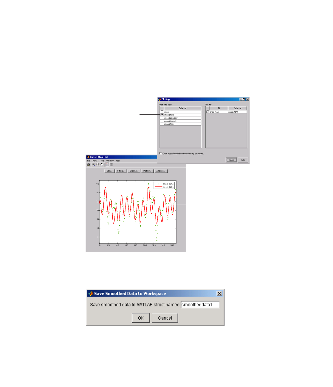
Use the Plotting GUI to display only the data sets of interest. As shown
below, the periodic structure of the ENSO data set becomes apparent when
it is smoothed using a moving average filter with the default span. Not
surprisingly, the uncovered structure is periodic, which suggests that a
reasonable parametric model should include trigonometric functions.
Display only the data set created
with the moving average method.
2-36
The smoothing process uncovers obvious
periodic structure in the data.
Saving the Results. By clicking the Save to workspace button, you can
save a smoothed data set as a structure to the MATLAB workspace. This
example saves the moving average results contained in the
enso (ma) data set.
Page 53

Preprocessing Data
The saved structure contains th e original predictor data x and the smoothed
data
y.
smootheddata1
smootheddata1 =
x: [168x1 double]
y: [168x1 double]
Excluding and Sectioning Data
• “Introduction” on page 2-37
• “Exclusion Rules” on page 2-38
• “Excluding Individual D a ta Points” on page 2-39
• “Excluding Data Sections in the Domain o r Range” on page 2-39
• “Marking Outliers” on page 2-39
• “Sectioning” on page 2-42
• “Example: Excluding and Sectioning Data” on page 2-44
Introduction
If there is justification, you might w ant to exclude part of a data set from a
fit. Typically, you exclude data so that subsequent fits are not adversely
affected. For example, if you a re fitting a parametric model to measured
data that has been corrupted by a faulty sensor, the resulting fit coefficients
will be inaccurate.
Curve Fitting Toolbox software providestwomethodstoexcludedata:
• Marking Outliers — Outliers are defined as individual data points that
you exclude because they are inconsistent with the statistical nature of
the bulk of the data.
• Sectioning — Sectioning excludes a window of response or predictor data.
For example, if many data points in a data set are corrupted by large
systematic errors, you might want to section them out of the fit.
2-37
Page 54

2 Interactive Curve Fitting
For each of these methods, you must create an exclusion rule, which captures
the range, domain, or index of the data points to be excluded.
To exclude data while fitting, you use the Fitting GUI to associate the
appropriate exclusion rule with the data set to be fit. Refer to “Example:
Robust Fitting” on page 2-68 for more information about fitting a data set
using an exclusion rule.
YoumarkdatatobeexcludedfromafitwiththeExcludeGUI,which
youopenfromCurveFittingTool. TheGUIisshownbelowfollowedby
a description of its features.
2-38
Exclusion Rules
• Exclusion rule name —Specifythenameoftheexclusionrulethat
identifies the data points to be excluded from subsequent fits.
• Existing exclusion rules — Lists the names of all exclusion rules created
during the current session. When you select an existing exclusion rule, you
can perform these actions:
- Click Copy to copy the exclusion rule. The exclusions associated with
the original exclusion rule are recreated in the GUI. You can modify
Page 55

Preprocessing Data
these exclusions and then click Create exclusion rule to save them to
the copied rule.
- Click Rename to change the name of the exclusion rule.
- Click Delete todeletetheexclusionrule. Toselectmultipleexclusion
rules, you can use the Ctrl key and the mouse to select exclusion rules
one by one, or you can use the Shift key and the mouse to select a range
of exclusion rules.
- Click View to display the exclusion rule graphically. If a data set is
associated with the exclusion rule, the data is also displayed.
Excluding Individual Data Points
• Select data set — Select the data set from which data points will be
marked as excluded. You must select a data set to exclude individual
data points.
• Exclude graphically — Open a GUI that allows you to exclude individual
data points graphically.
Individually excluded data points are marked by an “
automatically identified i n the Check to exclude point table.
• Check to exclude point — Select individual data points to exclude. You
can so rt this table by clicking on any of the column headings.
x”intheGUI,andare
ExcludingDataSectionsintheDomainorRange
• Section — Specify data to be excluded. You do not need to select a data set
to create an exclusion rule by sectioning.
- Exclude X — Specify beginning and ending intervals in the predictor
data to be excluded.
- Exclude Y — Specify beginning and ending intervals in the response
data to be excluded.
Marking Outliers
Outliers are defined as individual data points that you exclude from a fit
because they are inconsistent with the statistical nature of the bulk of the
2-39
Page 56

2 Interactive Curve Fitting
data, and will adversely affect the fit results. Outliers are often readily
identified by a scatter plot of response data versus predictor data.
Marking outliers with Curve Fitting Tool follows these rules:
• Youmustspecifyadatasetbefore creating an exclusion rule.
In gene ral, you should use the exclusion rule only with the specific data set
it was based on. However, the toolbox does not prevent you from using the
exclusion rule with another data set provided the size is the same.
• Using the Exclude GUI, you can exclude outliers either graphically or
numerically.
As described in “Parametric Fitting” on page 2-52, one of the basic
assumptions underlying curve fitting is that the data is statistical in nature
and is described by a particular distribution, which is often assumed to be
Gaussian. The statistical nature of the data implies that it contains random
variations along with a deterministic component.
2-40
data = deterministic component + random component
However, your data set might contain one or more data points that
are non-statistical in nature, or are described by a different statistical
distribution. These data points might be easy to identify, or they might be
buried in the data and difficult to identify.
A non-statistical process can involve the measurement of a physical variable
such as temperature or voltage in which the random variation is negligible
compared to the systematic e rrors. For example, if your sensor calibration
is inaccurate, the data measured with that sensor will be systematically
inaccurate. Insomecases,youmightbeabletoquantifythisnon-statistical
data component and correct the data accordingly. However, if the scatter plot
reveals that a handful of response values are far removed from neighboring
response values, these data points are considered outliers and should be
excluded from the fit. Outliers are usually difficult to explain away. For
example, it might be that your sensor experienced a power surge or someone
wrote down the wrong number in a log book.
If you decide there is justification, you should mark outliers to be excluded
from subsequent fits—particularly parametric fits. Removing these data
Page 57

Preprocessing Data
points can have a dramatic effect on the fit results because the fitting process
minimizes the square of the residuals. If you do not exclude outliers, the
resulting fit will be poor for a large portion of your data. Conversely, if you
do exclude the outliers and choose the appropriate model, the fit results
should be reasonable.
Because outliers can have a significant effect on a fit, they are considered
influential data. However, not all influential data points are outliers. Fo r
example, your data set can contain valid data points that are far removed
from the rest of the data. The data is valid because it is well described by
the model used in the fit. The data is influential because its exclusion will
dramatically affect the fit results.
Two ty pes of influential data points are shown below for generated data. Also
shown a re cubic polynomial fits and a robust fit that is resistant to outliers.
2-41
Page 58

2 Interactive Curve Fitting
Plot (a) shows that the two influential data points are outliers and adversely
affect the fit. Plot
consistent with the model and do not adversely affect the fit. Plot
that a robust fitting procedure is an acceptable alternative to marking
outliers for exclusion.
(b) shows that the two influential data points are
(c) shows
Sectioning
Sectioning involves specifying response or predictor data to exclude. You
might want to section a data set because different parts of the data set are
described by d ifferent models or are corrupted by noise, large systematic
errors, and so on.
Sectioning data with Curve Fitting Tool follows these rules:
• If you are only sectioning data and not excluding individual data points,
then you can create an exclusion rule without specifying a data set name.
• You can associate an exclusion rule with any data set provided that the
exclusion rule overlaps with the data. This is useful if you have multiple
data sets from which you want to exclude data points using the same rule.
2-42
• Use the Exclude GUI to create the exclusion rule.
• You can exclude vertical strips at the edges of the data, horizontal strips
at the edges of the data, or a border around the data. Refer to “Example:
Excluding and Sectioning Data” on page 2-44 for an example.
• To exclude multiple sections of data, you can use the
from the MATLA B command line.
excludedata function
Page 59

Preprocessing Data
Two example s of sectioning by domain are shown below for generated data.
The upper shows the data set sectioned by fit type. The section to the left of 4
is fit with a linear polynomial, as shown by the bold, dashed line. The section
to the right of 4 is fit with a cubic polynomial, as shown by the bold, solid line.
The lower plot shows the data set sectioned by fit type and by valid data.
Here, the right-most section is not part of any fit because the data is corrupted
by noise.
Note For illustrative purposes, the preceding figures have been enhanced
to show portions of the curves with bold markers. Curve Fitting Toolbox
software does not use bold markers in plots.
2-43
Page 60

2 Interactive Curve Fitting
Example: Excluding and Sectioning Data
ThisexamplemodifiestheENSOdatasettoillustrateexcludingand
sectioning data. First, copy the ENSO response data to a new variable and
add two outliers that are far removed from the bulk of the data.
yy = pressure;
yy(ceil(length(month)*rand(1))) = mean(pressure)*2.5;
yy(ceil(length(month)*rand(1))) = mean(pressure)*3.0;
Import the variables month and yy as the new data set enso1, and open the
Exclude GUI.
Assume that the first and last eight months of the data set are unreliable, and
should be excluded from subsequent fits. The simplest way to exclude these
data points is to section the predictor data. To do this, specify the data you
want to exclude in the Exclude Sections field of the Exclude GUI.
2-44
Therearetwowaystoexcludeindividualdatapoints: usingtheCheck to
exclude point table or graphica l ly. For this example, the simp le s t way to
exclude the outliers is graphically. To do this, select the data set name and
click the Exclude graphically button, which opens the Select Points for
Exclusion Rule G UI.
To mark data points for exclusion in the GUI, place the mouse cursor over
the data point and left-click. The excluded data point is marked with a red
Page 61

Preprocessing Data
x. To include an excluded data point, right-click the data point or select the
Includes Them radio button and left-click. Included data points are marked
with a blue circle. To select multiple data points, click the left mouse button
and drag the selection rubber band so that the rubber band box encompasses
the desired data points. Note that the GUI identifies sectioned data with gray
strips. You cannot graphically include sectioned data.
As shown below, the first and last eight months of data are excluded from
the data set by sectioning, and the two outliers are excluded graphically.
Note that the graphically excluded data points are identified in the Check to
exclude point table. If you decide to include an excluded data point using
the table, the graph is automatically updated.
If there are fits associated with the data, you can exclude data points based on
the residuals of the fit by selecting the residual data in the Y list.
2-45
Page 62

2 Interactive Curve Fitting
The Exclude GUI for this example is show n below.
To save the exclusion rule, click the Create exclusion rule button. To
exclude the data from a fit, you must select the exclusion rule from the Fitting
GUI. Because the exclusion rule created in this example uses individually
excluded data points, you can use it only with data sets that are the same
size as the ENSO data set.
2-46
Viewing the Exclusion Rule. To view the exclusion rule, select an existing
exclusion rule name and click the View button.
Page 63

Preprocessing Data
The View Exclusion Rule GUI shown below displays the modified ENSO data
set and the excluded data points, which are grayed in the table.
Missing V
Althoug
data, an
still wa
associ
For exa
line, y
numbe
To re
NaNs
doc
nt to remove this data from your data set. To do so, you modify the
ated data set variables from the MATLAB command line.
ou must supply predictor and response vectors that contain finite
rs. To remove
ind = find(isinf(xx));
xx(ind) = [];
yy(ind) = [];
move
and outliers from a data set, refer to “Missing Data” in the MATLAB
umentation.
alues and Outliers
h Curve Fitting Toolbox software ignores
d you can exclude outliers during the fitting process, you might
mple, when using toolbox functions such as
Infs,youcanusetheisinf function.
NaNs, you can use the isnan function. For examples that remove
InfsandNaNs when fitting
fit from the command
2-47
Page 64

2 Interactive Curve Fitting
Fitting Data
You fit data using the Fitting GUI. To open the Fitting GUI, click the Fitting
button from Curve Fitting Tool.
The Fitting GUI is shown below for the census data described in Chapter 1,
“Getting Started”, followed by the general steps you use when fitting any
data set.
2-48
Page 65

Fitting Data
1 Selectadatasetandfitname.
• Select the name of the current fit. When you click New fit or Copy fit,
a default fit name is automatically created in the Fit name field. You
can specify a new fit name by editing this fi eld.
2-49
Page 66

2 Interactive Curve Fitting
• Select the name of the current data set from the Data set list. All
imported and smoothed data sets are listed.
2 Select an exclusion rule.
If you want to exclude data from a fit, select an exclusion rule from the
Exclusion rule list. The list contains only exclusion rules that are
compatible with the current data set. An exclusion rule is compatible with
the current data set if their lengths are identical, or if it is created by
sectioning only.
3 Select a fit type and fit options, fit the data, and evaluate the goodness of fit.
• The fit type can be a library or custom parametric model, a smoothing
spline, or an interpolant.
• Select fit options such as the fitting algorithm, and coefficient starting
points and constraints. Depending on your data and model, accepting
the default fit options often produces an excellent fit.
• Fit the data by clicking the Apply button or by selecting the Immediate
apply check box.
2-50
• Examine the fitted curve, residuals, goodness of fit statistics, confidence
bounds, and prediction bounds for the current fit.
4 Compare fits.
• Compare the current fit and data set to previous fits and data sets by
examining the goodness of fit statistics.
• Use the Table Options GUI to modify w hich goodness of fit statistics are
displayed in the Table of Fits. You can sort the table by clicking on
any column heading.
5 Save the fit results.
If the fit is good, save the results as a structure to the MATLAB workspace.
Otherwise, modify the fit options or select another model.
For m ore information on model types, fit settings, and examples, see:
• “Parametric Fitting” on page 2-52
Page 67

• “Nonparametric Fitting” on page 2-106
Fitting Data
2-51
Page 68

2 Interactive Curve Fitting
Parametric Fitting
In this section...
“Introduction” on page 2-52
“Library Models” on page 2-53
“Specifying Fit Options” on page 2-58
“Example: Rational Fit” on page 2-62
“Example: Robust Fitting” on page 2-68
Introduction
Parametric fitting involves finding coefficients (parameters) for one or more
models that you fit to data. The data is assumed to be statistical in nature
and is divided into two components: a deterministic component and a random
component.
2-52
data = deterministic component + random component
The d eterministic component is given by a p arametric model and the random
component is often described as error associated with the data.
data = model + error
The model is a function of the independent (predictor) variable and one or
more coefficients. The error represents random variations in the data that
follow a specific probability distribution (usually Gaussian). The variations
can come from many different sources, but are always present at some level
when you are dealing with measured data. Systematic variations can also
exist, but they can lead to a fitted model that does not represent the data well.
The model coefficients often have physical significance. For example,
suppose you have collected data that corresponds to a single decay mode of a
radioactive nuclide, and you want to estimate the half-life (T
The law of radioactive d ecay states that the activity of a radioactive substance
decays exponentially in time. Therefore, the model to use in the fit is given by
)ofthedecay.
1/2
Page 69

Parametric Fitting
where y0is the number of nuclei at time t =0,andλ is the decay constant.
The data can be described by
Both y0and λ are coefficients that are estimated by the fit. Because T
1/2
=ln(2)/λ, the fitted v alue of the decay constant yields the fitted half-life.
However, because the data contains some error, the deterministic component
of the equation cannot be determined exactly from the data. Therefore, the
coefficients and half-life calculation will have some uncertainty associated
with them. If the uncertainty is acceptable,thenyouaredonefittingthedata.
If the uncertainty is not acceptable,thenyoumighthavetotakestepsto
reduce it either by collecting more data or by reducing measurement error
and collecting new data and repeating the m odel fit.
In other situations where there is no theory to dictate a model, you might also
modify the model by adding or removing terms, or substitute an entirely
different model.
Library Models
Curve Fitting Toolbox parametric library models are described below.
• “Exponentials” on page 2-54
• “Fourier Series” on page 2-54
• “Gaussian” on page 2-55
• “Polynomials” on page 2-55
• “Power Series” on page 2-56
• “Rationals” on page 2-56
• “Sum of Sines” on page 2-57
• “Weibull Distribution” on p ag e 2-58
2-53
Page 70

2 Interactive Curve Fitting
Exponentials
The toolbox provides a one-term and a two-term exponential model.
Exponentials are often used when the rate of change of a quantity is
proportional to the initial amount of the quantity. If the coefficient associated
with e is negative, y represents exponential decay. If the coefficient is positive,
y represents exponential growth.
For example, a single radioactive decay mode of a nuclide is described by a
one-term exponential. a is interpreted as the initial number of nuclei, b is the
decay constant, x is time, and y is the number of remaining nuclei after a
specific amount of time passes. If two decay modes exist, then you must use
the two-term exponential model. For each additional decay mode, you add
another exponential term to the model.
2-54
Examples of exponential growth include contagious diseases for which a cure
is unavailable, and biological populations whose growth is uninhibited by
predation, environmental factors, and so on.
Fourier Series
The Fourier series is a sum of sine and cosine functions that is used to
describe a periodic signal. It is represented in either the trigonometric form or
the e xponential form. The toolbox provides the trigonometric Fourier serie s
form shown below,
where a0models a constant (intercept) term in the data and is associated with
the i = 0 cosine term, w is the fundamental frequency of the signal,nis the
number o f terms (harmonics) in the series, and
.
Page 71

Parametric Fitting
For more information about the Fourier series, refer to “Fourier Transforms”
in the MATL AB documentation.
Gaussian
The Gaussian model is used for fitting peaks, and is given by the equation
where a is th
width, n is t
Gaussian p
For exampl
describe
eamplitude,b is the centroid (location), c is related to the peak
he number of peaks to fit, and
eaks are encountered in many areas of science and engineering.
e, line emission spectra and chemical concentration assays can be
d by G aussian peaks.
.
Polynomials
Polynom
where n +1istheorder of the polynomial, n is the degree of the polynomial,
and
degree gives the highest power of the predictor variable.
In this guide, polynomials are described in terms of their degree. For example,
a third-degree (cubic) polynomial is given b y
ial models are given by
. The order gives the number of coefficients to be fit, and the
lynomials are often used when a simple empirical model is required. The
Po
del can be used for interpolation or extrapolation, or it can be used to
mo
aracterize data using a global fit. For example, the temperature-to-voltage
ch
2-55
Page 72

2 Interactive Curve Fitting
conversion for a Type J thermocouple in the 0oto 760otemperature range is
described by a seventh-degree polynomial.
Note Ifyoudonotrequireaglobalparametric fit and want to maximize the
flexibility of the fit, piecewise polynomials might provide the best approach.
Refer to “Nonparametric Fitting” on p age 2-106 for more information.
The main advantages of polynomial fits include reasonable flexibility for
data that is not too complicated, and they are linear, which means the fitting
processissimple. Themaindisadvantage is that high-degree fits can become
unstable. A dditionally, polynomials of any degree can provide a good fit
within the data range, but can diverge wildly outside that range. Therefore,
you should exercise caution when extrapolating with polynomials. Refer
to “Determining the Best Fit” on page 2-9 for examples of good and poor
polynomial fits to census data.
Note that when you fit with high-degree polynomials, the fitting procedure
uses the predictor values as the basis for a matrix with very large values,
which can result in scaling problems. To deal with this, you should normaliz e
the data by centering it at zero mean and scaling it to unit standard deviation.
You normalize data by selecting the Center and scale X data check box on
the Fitting GUI.
2-56
Power Series
The toolbox provides a one-term and a two-term power series model.
Power series models are used to describe a variety of data. For example, the
rate at which reactants are consumed in a chemical reaction is generally
proportional to the concentration of the reactant raised to some power.
Rationals
Rational models are defined as ratios of polynomials and are given by
Page 73

Parametric Fitting
wherenisthed
isthedegreeo
coefficient associated with
denominator unique when the polynomial degrees are the same.
In this guide, rationals are described in terms of the degree of the
numerator/the degree of the denominator. For example, a quadratic/cubic
rational equation is given by
Like polynomials, rationals are often used when a simple empirical model
is required. The main advantage of rationals is their flexibility with data
that has complicated structure. The main disadvantage is that they become
unstable when the denominator is around zero. For an example that uses
rational polynomials of various de g rees, refer to “Example: Rational Fit”
on page 2-62.
egree of the numerator polynomial and
f the denominator polynomial and
is always 1. This makes the numerator and
,whilem
. Note that the
Sum of Sines
The sum of sines model is used for fitting periodic functions, and is given
by the equation
2-57
Page 74

2 Interactive Curve Fitting
where a is the amplitude, b is the frequency, and c is the phase constant for
each sine wave term. n is the number of terms in the series and
This equation is closely related to the Fourier series described previously. The
main difference is that the sum of sines equation includes the phase constant,
and does not include a constant (intercept) term.
.
Weibull Distribution
The Weibull distribution is widely used in reliability and l ife (failure rate)
data analysis. The toolbox provides the two-parameter Weibull distribution
where a is the scale param eter and b is the shape parameter. Note that there
is also a three-parameter Weibull distribution with x replaced by x–cwhere
c is the location parameter. Additionally, there is a one-parameter Weibull
distribution where the shape parameter is fixed and only the scale parameter
is fitted. To use these distributions, you must create a custom equation.
2-58
Curve Fitting Toolbox software does not fit Weibull probability distributions
to a sample of data. Instead, it fits curves to response and predictor data such
that the curve has the same shape as a Weibull distribution.
Specifying Fit Options
• “Introduction” on page 2-59
• “Fitting Method and Algorithm” on page 2-59
• “Finite Differencing Parameters” on page 2-60
• “Fit Convergence Criteria” on page 2-61
• “Coefficient Parameters” on page 2-61
Page 75

Parametric Fitting
Introduction
You specify fit options with the Fit Options GUI. The fit options for the
single-term exponential are shown below. The coefficient starting values and
constraints are for the census data.
The available GUI options depend on whether you are fitting your data using
a linear model, a nonlinear model, or a nonparametric fit type. All the options
described below are available for nonlinear models. Method, Robust,and
coefficient constraints (Lower and Upper) are available for linear models.
Interpolants and smoothing splines include Method, but no configurable
options.
Fitting Method and Algorithm
• Method — The fitting method.
The method is automatically selected based on the library or custom model
you use. For linear models, the method is LinearLeastSquares.For
nonlinear models, the method is NonlinearLeastSquares.
2-59
Page 76

2 Interactive Curve Fitting
• Robust — Specify whether to use the robust least-squares fitting method.
The values are
- Off — Do not use robust fitting (default).
- On — Fit with default robust method (bisquare weights).
- LAR — Fit by minimizing the least absolute residuals (LAR).
- Bisquare — Fit by minimizing the summed square of the residuals,
and down-weight outliers using bisquare weights. In most cases, this is
thebestchoiceforrobust fitting.
• Algorithm — Algorithm used for the fitting procedure:
- Trust-Region — This is the default algorithm and must be used if you
specify coefficient constraints.
- Levenberg-Marquardt — If the trust-region algorithm does not
produce a reasonable fit, and you do not have coefficient constraints, you
should try the Levenberg-Marquardt algorithm.
- Gauss-Newton — This algorithm is included for pedagogical reasons
and should be the last choice for most models and data sets.
2-60
Finite Differencing Parameters
• DiffMinChange — Minimum change in coefficients for finite difference
Jacobians. The default value is 10
• DiffMaxChange — Maximum change in coefficients for finite difference
Jacobians. The default value is 0.1.
Note that DiffMinChange and DiffMaxChange apply to
• Any nonlinear custom equation — that is, a nonlinear equation that you
write.
• Some, but not all, of the nonlinear equations provided with Curve Fitting
Toolbox software.
However, DiffMinChange and DiffMaxChange do not apply to any linear
equations.
-8
.
Page 77

Parametric Fitting
Fit Convergence Criteria
• MaxFunEvals — Maximum number of function (model) evaluations
allowed. The default value is 600.
• MaxIter — Maximum number of fit iterations allowed. The default value
is 400.
• TolFun — Termination tolerance used on s topping conditions involving
the function (model) value. The default value is 10
-6
.
• TolX — Termination tolerance used on stopping conditions involving the
coefficients. The default value is 10
-6
.
Coefficient Parameters
• Unknowns — Symbols for the unknown coefficients to be fitted.
• StartPoint — The coefficient starting values. The default values depend
on the model. For rational, Weibull, and custom models, default values are
randomly selected within the range [0,1]. For all other nonlinear library
models, the starting values depend on the data set and are calculated
heuristically.
• Lower — Lower bounds on the fitted coefficients. The bounds are used
only w ith the trust region fitting algorithm. The default lower bounds for
most library models are
unconstrained. However, a few models have finite default lower bounds.
For example, Gaussians have the width parameter constrained so that it
cannot be less than 0.
• Upper — Upper bounds on the fitted coefficients. The bounds are used
only with the trust region fitting algorithm. The default upper bounds
for all library models are
unconstrained.
-Inf, which indicates that the coefficients are
Inf, which indicates that the coefficients are
For more information about these fit options, refer to the Optimization
Toolbox documentation.
The d efault coefficient starting points a nd constraints f or library and custom
models are given below. If the starting points are optimized, then they are
calculated heuristically based on the current data set. Random starting
2-61
Page 78

2 Interactive Curve Fitting
points are defined on the interval [0,1] and linear models do not require
starting points.
If a model does not have constraints, the coefficients have neither a lower
bound nor an upper bound. You can override the default starting points and
constraints by providing your own values using the Fit Options GUI.
Default Starting Points and Constraints
Model Star ting Points Constraints
Custom linear N/A
Custom nonlinear
Exponentials
Fourier series
Random
Optimized
Optimized
Gaussians Optimized
Polynomials
Power series
N/A
Optimized
Rationals Random
Sum of sines Optimized
None
None
None
None
c
>0
i
None
None
None
b
>0
i
Weibull Random a, b >0
Note that the sum of sines and Fourier series models are particularly sensitive
to starting points, and the optimized values might be accurate for only a few
terms in the associated equations.
Example: Rational Fit
This example fits measured data using a rational model. The data describes
the coefficient of thermal expansion for copper as a function of temperature
in degrees kelvin.
2-62
To get started, load the thermal expansion data from the file
which is provided with the toolbox.
load hahn1
hahn1.mat,
Page 79

Parametric Fitting
The workspace now contains two new variables, temp and thermex:
•
temp is a vector of temperatures in degrees kelvin.
thermex is a vector of thermal expansion coefficients for copper.
•
Import these two variables into Curve Fitting Tool and name the data set
CuThermEx.
For this data set, you will find the rational equation that produces the best fit.
As described in “Library Models” on page 2-53, rational models are defined as
a ratio of polynomials
where n is the degree of the numerator polynomial and m is the degree of the
denominator polynomial. Note that the rational equations are not associated
with physical parameters of the data. Instead, they provide a simple and
flexible empirical model that you can use for interpolation and extrapolation.
2-63
Page 80
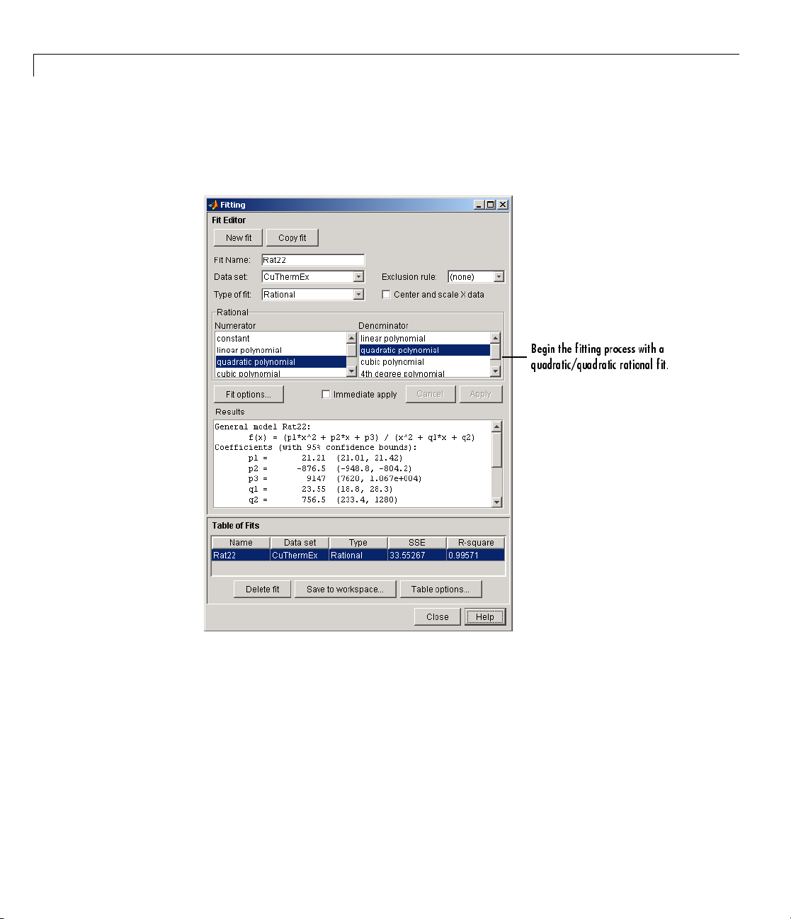
2 Interactive Curve Fitting
As you can see by examining the shape of the data, a reasonable initial choice
for the rational model is quadratic/quadratic. The Fitting GUI configured for
this equation is shown below.
2-64
Page 81

Parametric Fitting
The data, fit, and residuals are shown below.
The fit clearly misses
some of the data.
The residuals show a strong pattern
indicating a better fit is possible.
The fit clearly misses the data for the smallest and largest predictor values.
Additionally, the residuals show a strong pattern throughout the entire data
set indicating that a better fit is possible.
2-65
Page 82

2 Interactive Curve Fitting
For the next fit, try a cubic/cubic equation. The data, fit, and residuals are
shown below.
2-66
The numerical results shown below indicate that the fit did not converge.
Page 83

Parametric Fitting
Although the message in the Results window indicates that you might
improve the fit if you increase the maximum number of iterations, a better
choice at this stage of the fitting processistouseadifferentrationalequation
because the current fit contains several discontinuities. These discontinuities
are due to the function blowing up at predictor values that correspond to
the zeros of the denominator.
As the next try, fit the data using a cubic/quadratic equation. The data, fit,
and residuals are shown below.
The fit is well behaved over the entire data range, and the residuals are
randomly scattered about zero. Therefore, you can confidently use this fit
for further analysis.
2-67
Page 84

2 Interactive Curve Fitting
Example: Robust
This example fit
consists of the 2
Florida. The fi
linear least sq
In the 2000 pre
Florida, comp
they claim le
of the Democr
used only in P
presidenti
Beach is far
point shoul
To get star
flvote2k.
load flvote2k
The work
•
buchana
•
bush is
space n ow contains these three new variables:
s data that is assumed to contain one outlier. The data
000 United States presidential election results for the state of
t model is a first degree polynomial and the fit m ethod is robust
uares with bisquare weights.
sidential election, many residents of Palm Beach County,
lained that the design of the election ballot was confusing, which
d them to vote for the Reform candidate Pat Buchanan instead
atic candidate Al Gore. The so-called “butterfly ballot” was
alm Beach County and only for the election-day ballots for the
al race. As you will see, the number of Buchanan votes for Palm
removed from the bulk of data, which suggests that the data
d be treated as an outlier.
ted, load the Florida election result data from the file
mat
, which is provided with the toolbox.
n
is a vector of votes for the Reform Party candidate Pat Buchanan.
a vector of votes for the Republican Party candidate George Bush.
Fitting
2-68
•
gore is
Each v
count
the va
Bucha
vs. g
For t
pred
hanan votes =(bush votes)(m
buc
chanan votes =(gore votes)(m
bu
a vector of votes for the Democratic Party candidate Al Gore.
ariable contains 68 elements, which correspond to the 67 Florida
ies plus the absentee ballots. The names of the counties are given in
riable
nan votes as the response data:
ore
counties. From these variables, create two data sets with the
buchanan vs. bush and buchanan
.
his example, assume that the relationship between the response and
ictor data is linear with an offset of zero.
)
1
)
2
Page 85

Parametric Fitting
m1is the number of Bush votes expected for each Buchanan vote, and m2is
the number of Gore votes expected for each Buchanan vote.
To create a first-degree polynomial equation with zero offset, you must create
a custom linear equation.
1 In Curve F itting Tool, click Fitting.
2 In the Fitting GUI , click New fit.
3 Select Custom Equations from the Type of fit list, and click the New
buttontoopentheNewCustomEquationdialogbox.
4 To create a first degree polynomial with zero offset, on the Linear Equations
tab:
a Editthecoefficientnametom,andtheTerms to x.
b Clear the checkbox Unknown constant coefficient to remove the
constant term.
c Specify FlaEelection for the Equation name.
The Linear Equations tab of the New Custom Equation dialog box is
shown below.
2-69
Page 86

2 Interactive Curve Fitting
2-70
d Click OK.
Before fitting, you should exclude the data point associated with the absentee
ballots from each data set because these voters did not use the butterfly
ballot. As described in “Marking Outliers” on page 2-39, you can exclude
individual data points from a fit either graphically or numerically using the
Exclude GUI. For this example, you should exclude the data numerically. The
index of the absentee ballot data is given by
ind = find(strcmp(countie s,'Absentee Ball ots' ))
ind =
68
Page 87

In Cu rve Fitting Tool, click Exclude. The Exclude GUI is shown below.
1 Select the data set.
Parametric Fitting
2 Select the check box to exclude point 68.
3 Name the exclusion rule AbsenteeVotes.
4 Click Create exclusion rule.
5 Click Close.
Youwillassociatetheexclusionrulewiththedatasettobefittedwhenyou
return to the Fitting GUI.
For each data set, create a robust fit with bisquare weights using the
FlaElection equation defined above. For comparison purposes, also perform
a regular linear least-squares fit. F ollow these steps:
1 In the Fitting GUI, select the buchanon vs bush data set, the custom
equation fit type, and select the
FlaElection equation you defined
previously.
2 Select AbsenteeVotes in the Exclusion rule list.
2-71
Page 88

2 Interactive Curve Fitting
3 Click Fit Options and select Robust Bisquare. Close the Fit Options
dialog box.
4 Specify a meaningful fit name such as BBLinRobust.
5 Click Apply to save the changes to the fit (or select the Immediate apply
check box to avoid the need for this).
6 Click Copy fit and change the data set to buchanon vs gore to create a
similar robust fit to the other data set. Edit the fit name to
7 Forbothyourrobustfits,clickCopy fit and change the new fit’s Robust fit
option setting to
fit for comparison purposes. Edit the fit names to
Off. These two fits perform a regular linear least-squares
BBLin and BGLin.
BGLinRobust.
The Fit Editor and the Fit Options GUI are shown below for a robust fit.
2-72
Page 89

Parametric Fitting
The data, robust and regular least-squares fits, and residuals for the
buchanan vs. bus h data set only are shown below. Use the Plotting dialog
box to control what is shown in Curve Fitting Tool plots.
Click and hold a point in the Curve Fitting Tool plots to see the data tip. You
can identify the Palm Beach County data in the scatter plot by using the data
tips feature. The index number o f the data point for Palm Beach is 50.
ind = find(strcmp(countie s,'Palm Beach'))
ind =
50
The graphical results show that the linear model is reasonable for the majority
of data points, and the residuals appear to be randomly scattered around
zero. However, two residuals stand out. The largest residual corresponds to
Palm Beach County. The other residual is at the largest predictor value, and
corresponds to Miami/D ade County.
The numerical results are shown below. The inverse slope of the robust fit
indicates that Buchanan should receive one vote for e ve r y 197.4 Bush votes.
2-73
Page 90

2 Interactive Curve Fitting
The data, robust and regular least-squares fits, and residuals for the buchan an
vs. gore
data set are shown below.
2-74
Again, the graphical results show that the linear model is reasonable for the
majority of data points, and the residuals appear to be randomly scattered
around zero. However, three residuals stand out. The largest residual
corresponds to Palm Beach County. The other residuals are at the two largest
predictor values, and correspond to M iami/Dade County and Broward County.
The numerical results are shown below. The inverse slope of the robust fit
indicates that Buchanan should receive one vote for every 189.3 Gore votes.
Page 91

Parametric Fitting
Using the fitted slope value, you can determine the expected number of
votes that Buchanan should h ave received for each fit. For the Buchanan
versus Bush data, you evaluate the fit at a predictor value of 152,951. For
the Buchanan versus Gore data, you evaluate the fit at a predictor value of
269,732. These results are shown below for both data sets and both fits.
Expected Buchanan Votes in Palm Beach County
Expected Buchanan
Data Set Fit
Buchanan vs. Bush
Ordinary least squares
Robust least squares
Buchanan vs. Gore Ordinary least squares
Robust least squares
Votes
814
775
1246
1425
The robust results for the Buchanan versus Bush data suggest that Buchanan
received 3411 – 7 75 = 2636 excess votes, w hile robust results for the B uchanan
versus Gore data suggest that Buchanan received 3411 – 1425 = 1986 excess
votes.
The margin of victory for George Bush is given by
margin = sum(bush)-sum(go re)
margin =
537
Therefore, the voter intention comes into play because in both cases, the
margin of victory is less than the excess Buchanan votes.
In conclusion, the analysis of the 2000 United States presidential election
results for the state of Florida suggests that the Reform Party candidate
2-75
Page 92

2 Interactive Curve Fitting
received an excess number of votes in Palm Beach County, and that this excess
number was a crucial factor in determining the election outcome. However,
additional analysis is required before a final conclusion can be made.
2-76
Page 93

Creating Custom Models
In this section...
“Custom Models vs. Library Models” on page 2-77
“Creating Custom Models” on page 2-77
“Editing and Saving Custom Models” on page 2-81
“Example: Legendre Polynomial” on page 2-83
“Example: Fourier Series” on page 2-91
“Example: Gaussian with Exponential Background” on page 2-101
Custom Models vs. Library Models
If the toolbox library does not contain a desired parametric equation, you can
create your own custom equation. Library models, ho w e ver, offer the best
chance for rapid convergence. This is because:
Creating Custom Models
• For most library models, optimal default coefficient starting points are
calculated. For custom models, the default starting points are chosen at
random on the interval [0,1].
• Library models use an analytic Jacobian; custom models use finite
differencing.
• When using the Analysis GUI, library models use analytic derivatives and
integrals if the integral can be expressed in closed form; custom models use
numerical approximations.
Creating Custom Models
Create custom equations with the New Custom Equation G UI. Open the
GUI in one of two ways:
• From Curve Fitting Tool, select Tools > Custom Equation.
• From the Fitting GUI, select Custom Equations from the Type of fit list,
then click the New button.
2-77
Page 94

2 Interactive Curve Fitting
The GUI contains two panes: one for creating linear custom equations and
one for creating general (nonlinear) custom equations.
Linear Equations
Linear models are linear combinationsof(perhapsnonlinear)terms. They
are defined by equations that are linear in the parameters. Use the Linear
Equations pane on the New Custom Equation GUI to create custom linear
equations. Interface controls are described below.
2-78
• Independent variable — Symbol representing the independent
(predictor) variable. The default symbol is
x.
Page 95

Creating Custom Models
• Equation — Symbol representing the dependent (response) variable,
followed by the linear equation. The default symbol is
y.
- Unknown Coefficients — The unknown coefficients to be determined
by the fit. The default symbols are
a, b, c,andsoon.
- Terms — Functions of the independent variable. These may be
nonlinear. Terms may not contain a coefficient to be fitted.
- Unknown constant coefficient — If selected, a constant term
(y-intercept) is included in the equation. Otherwise, a constant term
is not included.
- Add a term — Add a term to the equation. An unknown coefficient is
automatically added for each new term.
- Remove last term — Remove the last term added to the equation.
• Equation name — The name of the equation. By default, the name is
automatically updated to be identical to the custom equation given by
Equation. If y ou override the default, the name is no longer automatically
updated.
General Equations
General models are, in general, nonlinear combinations of (perhaps
nonlinear) terms. They are defined by equations that may be nonlinear
in the parameters. Use the General Equations pane on the New Custom
Equation GUI to create custom general equations. Interface controls are
described below.
2-79
Page 96

2 Interactive Curve Fitting
2-80
• Independent variable — Symbol representing the independent
(predictor) variable. The default symbol is
• Equation — Symbol representing the dependent (response) variable,
followed by the general equation. The default symbol is
the terms of the equation, the unknown coefficients, associated starting
values, and constraints automatically populate the table. By default,
the starting values are randomly selected on the interval [ 0,1] and are
unconstrained.
You can immediately change the default starting values and constraints in
this table, or you can change them later using the Fit Options GUI.
• Equation name — The name of the equation. By default, the name is
automatically updated to be identical to the custom equation given by
x.
y.Asyoutypein
Page 97

Creating Custom Models
Equation. If y ou override the default, the name is no longer automatically
updated.
Note If you use the General Equations panetodefinealinearequation,a
nonlinear fitting procedure is used. While this is allowed, it is inefficient, and
canresultinlessthanoptimalfittedcoefficients. UsetheLinear Equations
pane to define custom linear equations.
Editing and Saving Custom Models
When you click OK on the New Custom Equation GUI, the displayed
Equation name is saved for the current session in the Custom Equations
list on the Fitting GUI. The list is highlighted in the picture of the Fitting
GUI below.
2-81
Page 98

2 Interactive Curve Fitting
2-82
Page 99

Creating Custom Models
To edit a custom equation, select the equation in the Custom Equations list
and click the Edit button. The Edit Custom Equation GUI appears. The
Edit Custom Equation GUI is identical to the New Custom Equation GUI,
but is pre-populated with the selected equation. After editing an equation
in the Edit Custom Equation GUI, click OK to save it back to the Custom
Equations list for further use in the current session. A button to Copy
and Edit is also available, if you want to save both the original and edited
equations for the current session.
To save custom equations for future sessions, select the File > Save Session
menu item in Curve Fitting Tool.
Example: Legendre Polynomial
This example fits data using several custom linear equations. The data is
generated, and is based on the nuclear reaction
use sums of Legendre polynomial te rms.
12
C(e,e’α)8Be. The equations
Consider an experiment in which 124 MeV electrons are scattered from
12
C
nuclei. In the subsequent reaction, alpha particles are emitted and produce
the residual nuclei
8
Be. By analyzing the number of alpha particles emitted as
a function of angle, you can deduce certain information regarding the nuclear
dynamics of
12
C. The reaction kinematics are shown below.
The data is collected by placing solid state detectors at values of Θαranging
from 10
o
to 240oin 10oincrements.
2-83
Page 100

2 Interactive Curve Fitting
It is sometimes useful to describe a v ariable expressed as a function of angle
in terms of Legendre polynomials
where Pn(x) is a Legendre polynomial of degree n, x is cos(Θα), and anare th e
coefficients of the fit. Refer to the
legendre function for information about
generating Legendre polynomials.
For the alpha-emission data, you can directly associate the coefficients with
the nuclear dynamics by invoking a theoretical model. Additionally, the
theoretical model introduces constraints for the infinite sum shown above.
In particular, by considering the angular momentum of the reaction, a
fourth-degree Legendre polynomial using only even terms should describe the
data effectively.
You can generate Legendre polynomials with Rodrigues’ formula:
2-84
The Legendre polynomials up to fourth degree are given below.
Legendre PolynomialsuptoFourthDegree
nP
0
(x)
n
1
1 x
2
3
4
(1/2)(3x
(1/2)(5x
(1/8)(35x
2
–1)
3
–3x)
4
–30x2+3)
You will fit the data using a fourth-degree Legendre polynomial with only
even terms:
 Loading...