Mathworks CONTROL SYSTEM TOOLBOX 9 user guide

Download

Control System Too

Getting Started Guide

lbox™ 9

How to Contact MathWorks

www.mathworks. comp.soft-sys.matlab Newsgroup www.mathworks.com/contact_TS.html Technical Support

suggest@mathworks.com Product enhancement suggestions

bugs@mathwo doc@mathworks.com Documentation error reports service@mathworks.com Order status, license renewals, passcodes

info@mathwo

com

rks.com

Web

Bug reports

Sales, prici

ng, and general information

508-647-7000 (Phone)

508-647-7001 (Fax)

The MathWorks, Inc. 3 Apple Hill Drive Natick, MA 01760-2098

For contact information about worldwide offices, see the MathWorks Web site.

Control System Toolbox™ Getting Started Guide

The software desc ribed in this document is furnished under a license agreeme nt. The software may be used or copied only under the terms of the license agreement. No part of this manual may be photocopied or reproduced in any form without prior written consent from The MathWorks, Inc.

FEDERAL ACQUISITION: This provision applies to all acquisitions of the Program and Documentation by, for, or through the federal government of the United States. By accepting delivery of the Program or Docum entation, the government hereby agrees that this software or documentation qualifies as commercial computer software or commercial computer software documentation as such terms are used or defined in FAR 12.212, DFARS Part 227.72, and DFARS 252.227-7014. Accordingly, the terms and conditions of this Agreement and only those rights specified in this Agreement, shall pertain to and govern theuse,modification,reproduction,release,performance,display,anddisclosureoftheProgramand Documentation by the federal government (or other entity acquiring for or through the federal governme nt) and shall supersede any conflicti ng contractual terms or conditions. If this License fails to meet the government’s needs or is inconsistent in any respect with federal procurement law, the government agrees to return the Program and Documentation, unused , to The MathWorks, Inc.

Trademarks

MATLAB and Simulink are registered trademarks of The M athWorks, Inc. See

www.mathworks.com/trademarks for a list of additional trademarks. Other product or brand

names may be trademarks or registered trademarks of their respective holders.

Patents

MathWorks products are protected by one or more U.S. patents. Please see

www.mathworks.com/patents for more information.

Revision History

November 2002 First printing New Version 5.0 (Release 12) June 2001 Second printing Revised for Version 5.1 (Release 12.1) July 2002 Online only Revised for Version 5.2 (Release 13) June 2004 Online only Revised for Version 6.0 (Release 14) March 2005 Online only Revised for Version 6.2 (Release 14SP2) September 2005 O nline only Revised for Version 6.2.1 (Release 14SP3) March 2006 Online only Revised for Version 7.0 (Release 2006a) September 2006 Online only Revised for Version 7.1 (Release 2006b) March 2007 Online only Revised for Version 8.0 (Release 2007a) September 2007 O nline only Revised for Version 8.0.1 (Release 2007b) March 2008 Online only Revised for Version 8.1 (Release 2008a) October 2008 Third printing Revised for Version 8.2 (Release 2008b) March 2009 Online only Revised for Version 8.3 (Release 2009a) September 2009 Online only Revised for Version 8.4 (Release 2009b) March 2010 Online only Revised for Version 8.5 (Release 2010a) September 2010 Online only Revised for Version 9.0 (Release 2010b)

Contents

Product Overview

Why Use This Too

Using the Docu

Related Prod

mentation

ucts

lbox?

.............................

..........................

..................................

Building M

Linear (LTI) Models ................................ 2-2

What Is a Plant? Linear Model Representations SISO Example: The DC Motor Building SISO Models Constructing Discrete Time Systems Adding Delays to Linear Models LTI Objects

MIMO Models

MIMO Example: State-Space Model of Jet Transport

Aircraft Constructing MIMO Transfer Functions Accessing I/O Pairs in MIMO Systems

.................................. 2-2

....................... 2-2

....................... 2-3

.............................. 2-6

.................. 2-9

..................... 2-10

...................................... 2-10

..................................... 2-13

....................................... 2-13

............... 2-15

................ 2-17

1-2

1-3

1-4

odels

Arrays of Linear Models

Model Characteristics

Interconnecting Linear Models

............................ 2-18

.............................. 2-21

..................... 2-23

Arithmetic Operations for Interconnecting Models ...... 2-23

Feedback Interconnections

Converting Between Continuous- and Discrete- Time

Systems

Available Commands for Continuous/Discrete

Conversion Available Methods for Continuous/Discrete Conversion Digitizing the Discrete DC Motor Model

........................................ 2-26

..................................... 2-26

.......................... 2-24

.. 2-26

............... 2-26

Reducing Model Order

Model Order Reduction Commands Techniques for Reducing Model Order Example: Gasifier Model

............................. 2-29

................... 2-29

................. 2-29

........................... 2-30

Analyzing Models

Quick Start for Performing Linear Analysis Using the

LTI Viewer

Plot Types Available in the LTI Viewer Example: Time and Frequency Responses of the DC

Motor Right-Click Menus Displaying Response Characteristics on a Plot Changing Plot Type Showing Multiple Response Types Comparing Multiple Models

...................................... 3-2

........................................ 3-7

................ 3-7

......................................... 3-8

................................ 3-10

................................ 3-14

.................... 3-16

......................... 3-17

.......... 3-11

vi Contents

Simulating Models with Arbitrary Inputs and Initial

Conditions

What is the Linear Simulation Tool? Opening the Linear Simulation Tool Working with the Linear Simulation Tool Importing Input Signals Example: Loading Inputs from a Microsoft

Spreadsheet

...................................... 3-22

.................. 3-22

.............. 3-23

............................ 3-26

Excel

.................................... 3-28

Example: Importing Inputs from the Workspace ........ 3-29

Designing Input Signals Specifying Initial Conditions

............................ 3-33

........................ 3-35

Functions for Time and Frequency Response

When to Use F unctions for Time and Frequency

Response Time and Frequency Response Functions Plotting MIMO Model Responses Data Markers Plotting and Comparing Multip le Systems Creating Custom Plots

...................................... 3-37

.............. 3-37

..................... 3-40

.................................... 3-42

............................. 3-47

........ 3-37

............. 3-44

Designing Compensators

Designing PID Controllers ......................... 4-2

Designing PID Controllers with the PID Tuner GUI Designing PID Controllers at the Command Line

SISO Design Tool

Quick Start for Tuning Compensator Parameters Using the

SISO Design Tool Components of the SISO Tool Design Options in the SISO Tool Opening the SISO Design Tool Using the SISO Design Task Node in the Control and

Estimation Tools Manager Importing Models into the SISO Design Tool Feedback Structure Analysis Plots for Loop Responses Using the Graphical Tuning Window Exporting the Compensator and Models Storing and Retrieving Intermediate Designs

.................................. 4-15

............................... 4-15

........................ 4-26

..................... 4-26

....................... 4-27

........................ 4-29

................................ 4-34

.................... 4-36

................. 4-42

............... 4-49

....... 4-14

........... 4-30

........... 4-51

..... 4-2

Bode Diagram Design

What Is Bode Diagram Design? Example: DC Motor Adjusting the Compensator Gain

.............................. 4-55

............................... 4-55

...................... 4-55

..................... 4-56

vii

Adjusting the Bandwidth ........................... 4-57

Adding an Integrator Adding a Lead Network Moving Compensator Poles and Zeros Adding a Notch Filter Modifying a Prefilter

.............................. 4-59

............................ 4-63

................. 4-68

.............................. 4-71

............................... 4-76

Root Locus Design

What Is Root Locus Design? Example: Electrohydraulic Servomechanism Changing the Compensator Gain Adding Poles and Zeros to the Compensator Editing Compensator Pole and Zero Locations Viewing Damping Ratios

Nichols Plot Design

What Is Nichols Plot Desig n? DC Motor Example Opening a Nichols Plot Adjusting the Compensator Gain Adding an Integrator Adding a Lead Network

Automated Tuning Design

Supported Automated Tuning Methods Loading and Displaying the DC Motor Example for

Automated Tuning

Applying Automated PID Tuning

Multi-Loop Compensator Design

When to Use Multi-Loop Compensator Design Workflow for Multi-Loop Compensator Design Example: Position Control of a DC Motor

................................. 4-81

......................... 4-81

..................... 4-88

............ 4-91

........................... 4-100

................................ 4-103

........................ 4-103

................................ 4-103

............................. 4-104

..................... 4-105

.............................. 4-108

............................ 4-110

.......................... 4-114

................ 4-114

.............................. 4-114

..................... 4-116

.................... 4-120

.............. 4-120

........... 4-82

.......... 4-96

.......... 4-120

viii Contents

Control Design Analysis of Multiple Models

Multiple Models Represent Sy stem Variations Control Design Analysis Using the SISO Design Tool Specifying a Nominal Model Frequency Grid for Multimodel Computations How to Analyze the Controller Design for Multiple

Models

........................................ 4-137

......................... 4-133

.......... 4-132

.... 4-132

.......... 4-136

Functions for Compensator Design .................. 4-147

When to Use Functions for Compensator Design Root Locus Design Pole Placement Linear-Quadratic-Gaussian (LQG) Design Example — Designing an LQG Regulator Example — Designing an LQG Servo Controller Example—DesigninganLQRServoControllerin

Simulink

................................. 4-147

................................... 4-148

.............. 4-162

...................................... 4-168

........ 4-147

............. 4-151

........ 4-165

Index

x Contents

Product Overview

• “Why Use This Toolbox?” on page 1-2

• “Using the Documentation” on p age 1-3

• “Related Products” on page 1-4

1 Product Overview

Why Use This Toolbox?

The Control System Toolbox™ product extends the MATLAB®software to provide functions designed specifically for control engineering.

This toolbox lets you construct and analyze linear models of dynamic systems. Use Control System Toolbox functions to model dynamic systems as transfer functions, in state-space form, or as arrays of frequency response data. Plot the time and frequency responses of your system to understand how your system behaves.

You can also use the toolbox to design and tune single-loop or multiple -loop control systems using various classical and state-space techniques.

1-2

Using the Documentation

If you are new to Control System Toolbox, review the Control System Toolbox Getting Started Guide to learn how to:

• Build and manipulate linear time-invariant models of dynamical systems

• Analyze such models and plot their time and frequency responses

• Design compensators using root locus and pole placement techniques

This guide also discusses model order reduction and linear quadratic Gaussian (LQG) control design techniques with examples.

Other documentation available for this toolbox includes:

• Release Notes — Highlights new and changed features in the latest product

release.

• Creating and Manipulating Models — In-depth information about creating,

manipulating, and analyzing linear models and linear time-invariant

(LTI) arrays. You can use LTI arrays to store collections of linear models

in one variable.

Using the Documentation

• Customization — Information about setting plot properties, including

setting preferences that persist from session to session.

• Control System Toolbox Design Case Studies —Workedexamples

of control design problems, including Kalman filtering and

Linear-Quadratic-Gaussian design. The examples illustrate

design techniques in both single-input/single-output (SISO) and

multiple-input/multiple-output (MIMO) systems.

• Control System Toolbox Reliable Computations — Discussion of numerical

stability and accuracy in computation

• Using the SISO Design Tool and the LTI Viewer — Complete descriptions

of the LTI Viewer and SISO Design Tool. These tools help you analyze

systems and design SISO compensators.

• Function Reference — D escribes the purpose, syntax, and options for each

function.

1-3

1 Product Overview

Related Products

ThefollowingtablesummarizesMathWorks®products that extend and complement the Control System Toolbox software. For current information about these products and other MathWorks products, point your Web browser to:

www.mathworks.com

Product

ulink

Control Design™

Simulink

Fuzzy Logic Toolbox™

Model Predictive Control Toolbox™

Robust Control Toolbox™

Sim

Description

Provides blocks for simulating models you create and analyze using the Control System Toolbox software.

Complements Control System Toolbox software with tools for modeling complex systems based on fuzzy logic.

Helps you design and simulate model predictive controllers for linear plant models created using Control System Toolbox functions.

Helps syste creat Tool to as conf mod

Let lin tu

you design robust control ms based on plant models ed using the Control System

box software. Enables you

sess robustness based on

idence bounds for your plant

els.

s y ou use Control System Toolbox

ear control to ols to analyze and

ne Simulink models.

1-4

Building Models

• “Linear (LTI) Models” on page 2-2

• “MIMO Models” on page 2-13

• “Arrays of Linear Models” on page 2 -18

• “Model Characteristics” on page 2-21

• “Interconnecting Linear Models” on page 2-23

• “Converting Between Continuous- and Discrete- Time Systems” on page

2-26

• “Reducing Model Order” on page 2-29

2 Building Models

Linear (LTI) Models

In this section...

“What Is a Plant?” on page 2-2

“Linear Model Representatio ns” on page 2-2

“SISO Example: The DC Motor” on page 2-3

“Building SISO M odels ” on page 2-6

“Constructing Discrete Time Systems” on page 2-9

“Adding Delays to Linear Models” on page 2-10

“LTI Objects” on page 2-10

What Is a Plant?

Typically, control engineers begin by developing a mathematical description of thedynamicsystemthattheywanttocontrol. Thesystemtobecontrolledis called a plant. As an example of a plant, this section uses the DC motor. This section develops the differential equations that describe the electromechanical properties of a DC motor with an inertial load. It then shows you how to use the Control System Toolbox functions to build linear models based on these equations.

2-2

Linear Model Representations

You can use Control Sy stem Toolbox functions to create the follow ing model representations:

• State-space models (SS) of the form

Ax Bu

yCxDu

where A, B, C,andD are matrices of appropriate dimensions, x is the state vector, and u and y are the input and output vectors.

• Transfer functions (TF), for example,

Linear (LTI) Models

()=

• Zero-pole-gain (ZPK) models, for exam ple,

()

• Frequency response data (FRD) models, which consist of sampled

measurements of a system’s frequency response. For example, you can store experimentally collected frequency response data in an FRD model.

Note The design of FRD models is a specialized subject that this guide does not address. See “Creating Frequency Response Data (FRD) Models” for a discussion of this topic.

++210

zjzj

()()

++ +−

(.)(.)

02 01

SISO Example: The DC Motor

A simple model of a DC motor driving an inertial load shows the angular rate

ω()t

of the load, ultimate goal of this example is to control the angular rate by varying the applied voltage. This figure shows a simple model of the DC motor.

A Simple Model of a DC Motor Driving an Inertial Load

, as the output and applied voltage,

t()

,astheinput. The

app

2-3

2 Building Models

In this model, the dynamics of the motor itself are idealized; for instance, themagneticfieldisassumedtobeconstant. Theresistanceofthecircuit is denoted by R and the self-inductance of the armature by L. If you are unfamiliar with the basics of DC motor modeling, consult any basic text on physical modeling. With this simple model and basic laws of physics, it is possible to develop differential equations that d escri be the behavior of this electromechanical system. In this example, the relationships between electric potential and mechanical force are Faraday’s law of induction and Ampère’s law for the force on a conductor moving through a magnetic field.

Mathematical Derivation

The torqueτseen at the shaft of the motor is proportional to the current i induced by the applied voltage,

τ() ()tKit

where Km, the armature constant, is related to physical properties of the motor, such as magnetic field strength, the number of turns of wire around

2-4

the conductor coil, and so on. The back (induced) electromotive force, a voltage proportional to the angular rate

υω

tKt() ()=

emf b

where Kb, the emf constant, also depends on certain physical properties of the motor.

The mechanical part of the motor equations is derived using Newton’s law, which states that th e inertial load J times the derivative of angular rate equals the sum of all the torques about the motor shaft. The result is this equation,

==− +

∑

where

Finally, the electrical part of the motor equations can be described by

Kfω

is a linear approximation for viscous friction.

KtKit

τω() ()

if m

seen at the shaft,

emf

,is

Linear (LTI) Models

υυ

ttL

app emf

di dt

Ri t() () ()−=+

or, solving for the applied voltage and substituting for the back emf,

υω

app b

Ri t K t() () ()=++

This sequence of equations leads to a set of two differential equat ions that describe the behavior of the motor, the first for the induced current,

di dt

=− − +() () ()ωυ

app

and the second for the resulting angular rate,

KtJKit

ω=− +

() ()

dt J

State-Space Equations for the DC Motor

Given the two differential equations derived in the last section, you can now develop a state-space representation of the DC motor as a dynamic system. The current i and the angular rate ω are the two states of the system. The

applied voltage,

, is the input to the system, and the angular velocity

app

ω is the output.

⎡

−−

⎢

⎡

⎤

⎢

ωω

⎣

() ()=

State-Space Representation of the DC Motor Exam ple

⎢

⎥

⎢

⎦

⎢

⎣

⎡

⋅

[]

⎢ ⎣

−

⎤ ⎥

⎦

[]

⎤

⎥

⎡

⎥

⋅

⎢

⎥

⎣

⎥ ⎦

⋅01 0ωυ

app

⎤

⎡

⎤

⎥⎥

⎢

⋅υ

⎥

⎢

⎦

⎥

⎢

⎦

⎣

app

t()

2-5

2 Building Models

Building SISO Mo

After you develo can construct SI

p a set of differential equations that describe your plant, you SO models using simple commands. The following sections

dels

discuss

• Constructing

• Converting be

• Creating tra

a state-space model of the DC motor

tween model representations

nsfer function and zero/pole/gain models

Constructing a State-Space Model of the DC Motor

Enter the fo

R= 2.0 % Ohms L= 0.5 % Henrys Km = .015 % torque constant Kb = .015 % emf constant Kf = 0.2 % Nms J= 0.02 % kg.m^2

Given th represe

A = [-R/L -Kb/L; Km/J -Kf/J] B = [1/L; 0]; C = [0 1]; D = [0]; sys_dc = ss(A,B,C,D)

llowing nominal values for the various parameters of a DC motor.

ese values, you can construct the numerical state-space

ntation using the

ss function.

2-6

These

commands return the following result:

x1 x2 x1 -4 -0.03 x2 0.75 -10

Linear (LTI) Models

x1 2 x2 0

x1 x2 y101

u1 y1 0

Converting Between Model Representations

Now that you have a state-space representation of the DC motor, y ou can convert to other model representations, including transfer function (TF) and zero/pole/gain (ZPK) models.

Transfer Function Representation. You can use

tf to convert from the

state-space representation to the transfer function. For example, use this code to convert to the transfer function representation of the DC motor.

sys_tf = tf(sys_dc)

Transfer fu nction:

1.5

-----------------s^2 + 14 s + 40.02

Zero/Pole/Gain Representation. Similarly, the zpk function converts from state-space or transfer function representations to the zero/pole/gain format. Use this code to convert from the state-space representation to the zero/pole/gain form for the DC motor.

sys_zpk = zpk(sys_dc)

Zero/pole/gain:

1.5

2-7

2 Building Models

------------------(s+4.004) ( s+9.996)

Note The state-space representation is best suited for numerical computations. For highest accuracy, convert to state space prior to combining models and avoid the transfer function and zero/pole/gain representations, except for model specif ication and inspection. See Reliable Computations for more information on numerical issues.

Constructing Transfer Function and Zero/Pole/Gain Models

In the DC motor example, the state-space approach produces a set of matrices that represents the model. If you choose a different approach, you can construct the corresponding models using

sys = tf(num,den) % Transfer function sys = zpk(z,p,k) % Zero/pol e/gain sys = ss(a,b,c,d) % State-sp ace sys = frd(response,fre quencies) % Frequency response data

tf, zpk, ss,orfrd.

2-8

For example, you can create the transfer function by specifying the numerator and denominator with this code.

sys_tf = tf(1.5,[1 14 40.02])

Transfer fu nction:

1.5

-----------------s^2 + 14 s + 40.02

Alternatively, if you want to create the transfer function of the DC motor directly, use these commands.

s = tf('s'); sys_tf = 1.5/(s^2+14*s +40.02)

These commands result in this transfer function.

Transfer f unction:

Linear (LTI) Models

1.5

-------------------s^2 + 14 s + 40.02

To build the zero/pole/gain model, use this command.

sys_zpk = zpk([],[-9. 996 -4.004], 1.5)

This command returns the following zero/pole/gain re pre sentation.

Zero/pole/gain:

1.5

------------------(s+9.996) ( s+4.004)

Constructing Discrete Time Systems

The Control System Toolbox software provides full support for discrete-time systems. You can create discrete systems in the same way that you create analog systems; the only difference is that you must specify a sample time period for any model you build. For example,

sys_disc = tf(1, [1 1], .01);

creates a SISO model in the transfer function format.

Transfer f unction:

----z+1

Sampling ti me: 0.01

Adding Time Delays to Discrete-Time Models

Youcanaddtimedelaystodiscrete-timemodelsbyspecifyinganinputdelay, output delay, or I/O delay when building the model. The time delay m ust be a nonnegative integer that represen ts a multiple of the sampling time. For example,

sys_delay = tf(1, [1 1], 0.01,'ioDelay',5)

2-9

2 Building Models

returns a system with an I/O delay of 5 s.

Transfer f unction:

z^(-5) * -----

z+1

Sampling ti me: 0.01

Adding Delays to Linear Models

You can add time delays to linear models by specifying an input delay, output delay, or I/O delay when building a m odel. F or example, to add an I/O delay to the DC motor, use this code.

sys_tfdelay = tf(1.5, [1 14 40.02],'ioDelay',0.05 )

This command constructs the DC motor transfer function, but adds a 0.05 second delay.

2-10

Transfer f unction:

1.5

exp(-0.05*s) * ------- -----------

s^2 + 14 s + 40.02

For a complete description of adding time de lays to models and closing loops with time delays, see Time Delays.

LTI Objects

For convenience, the Control System Toolbox software uses custom data structures called LTI objects to store model-related data. For example, the variable There are also TF, ZPK, and FRD objects for transfer function, zero/pole/gain, and frequency data response models respectively. The four LTI objects encapsulate the model data and enable you to manipulate linear systems as single entities rather than as collections of vectors or matrices.

To see what LTI objects contain, use the the contents of

sys_dc created for the DC motor example is called an SS object.

get command. This code describes

sys_dc from the DC motor example.

get(sys_dc)

a: [2x2 double] b: [2x1 double] c: [0 1] d: 0 e: []

StateName: {2x1 cell}

InternalDelay: [0x1 do uble]

Ts: 0

InputDelay: 0

OutputDelay: 0

InputName: {''} OutputName: {''} InputGroup: [1x1 struct ]

OutputGroup: [1x1 st ruct]

Name: ''

Notes: {}

UserData: []

Linear (LTI) Models

You can manipulate the data contained in LTI o bjects using the set command; see the Control System Toolbox online reference pages for descriptions of

set and get.

Another convenient way to set or retrieve LTI model properties is to access them directly using dot notation. For example,ifyouwanttoaccessthevalue of the

A matrix, instead of using get,youcantype

sys_dc.a

at the MATLAB prompt. This notation returns the A matrix.

ans =

-4.0000 -0.0300

0.7500 -10.0000

Similarly, if you want to change the values of the A matrix, you can do so directly, as this code show s.

A_new = [-4.5 -0.05; 0.8 -12.0];

2-11

2 Building Models

sys_dc.a = A_new;

For more information on LTI properties, type ltiprops at the MATLAB prompt. F or a complete description of LTI objects, see Creating and Manipulating Models.

2-12

MIMO Models

In this section...

“MIMO Example: State-Space Model of Jet Transport Aircraft” on page 2-13

“Constructing MIMO Transfer Functions” on page 2-15

“Accessing I/O Pairs in MIMO Systems” on page 2-17

MIMO Example: State-Space Model of Jet Transport Aircraft

You can use the same functions that apply to SISO systems to create multiple-input, multiple-output (MIMO) models. This example shows how to build a MIMO model of a jet transport. Because the development of a physical model for a jet aircraft is lengthy, only the state-space equations are presented here. See any standard text in aviation for a more complete discussion of the physics behind aircraft flight.

MIMO Models

The jet model during cruise flight at MACH = 0.8 and H = 40,000 ft. is

A = [-0.0558 -0.9968 0.0802 0.0415

0.5980 -0.1150 -0.0318 0

-3.0500 0.3880 -0.4650 0 0 0.0805 1.0000 0];

B = [ 0.0073 0

-0.4750 0.0077

0.1530 0.1430 00];

C=[0100

0001];

D=[0 0

00];

Use the following commands to specify this state-space model as an LTI object and attach names to the states, inputs, and outputs.

2-13

2 Building Models

states = {'beta' 'yaw' 'roll' 'phi'}; inputs = {'rudder' 'aileron'}; outputs = {'yaw rate' 'bank angle'};

sys_mimo = ss(A,B,C,D, 'statename',states,... 'inputname',inputs,... 'outputname',outputs);

You can display the LTI model by typing sys_mimo.

sys_mimo

beta yaw roll phi

beta -0.0558 -0.9968 0.0802 0.0415

yaw 0.598 -0.115 -0.0318 0

roll -3.05 0.388 -0.465 0

phi 0 0.0805 1 0

2-14

rudder ailer on

beta 0.0073 0

yaw -0.475 0.0077

roll 0.153 0.143

phi00

beta yaw roll phi

yawrate0100

bankangle0001

rudder ailer on

yawrate00

bank angle 0 0

Continuous-time model.

MIMO Models

The model has two inputs and two outputs. The units are radians for beta (sideslip angle) and phi (bank angle) and radians/sec for yaw (yaw rate) and

roll (roll rate). The rudde r and aileron deflections are in degrees.

As in the SISO case, use

tf(sys_mimo)

Transfer fu nction from input "rudder" to output...

yaw rate: ---------------------------------------------------

s^4 + 0.6358 s^3 + 0.9389 s^2 + 0.5116 s + 0.003674

bank angl e: ---------------------------------------------------

Transfer fu nction from input "aileron" to output...

0.0077 s^3 - 0.0005372 s^2 + 0.008688 s + 0.004523

yaw rate: ---------------------------------------------------

s^4 + 0.6358 s^3 + 0.9389 s^2 + 0.5116 s + 0.003674

bank angl e: ---------------------------------------------------

tf to derive the transfer function representation.

-0.475 s ^3 - 0.2479 s^2 - 0.1187 s - 0.05633

0.1148 s ^2 - 0.2004 s - 1.373

s^4 + 0.6358 s^3 + 0.9389 s^2 + 0.5116 s + 0.003674

0.1436 s^ 2 + 0.02737 s + 0.1104

s^4 + 0.6358 s^3 + 0.9389 s^2 + 0.5116 s + 0.003674

Constructing MIMO Transfer Functions

MIMO tra nsfer functions are two-dimensional arrays of elementary SISO transferfunctions. TherearetwowaystospecifyMIMOtransferfunction models:

• Concatenation of SISO transfer function models

• Using

tf with cell array arguments

Concatenation of SISO Models

Consider the following single-input, two-output transfer function.

2-15

2 Building Models

⎡ ⎢

()=

⎢

⎣

You can specify H(s) by concatenation of its SISO entries. For instance,

h11 = tf([1 -1],[1 1]); h21 = tf([1 2],[1 4 5]);

or, equivalently,

s = tf('s') h11 = (s-1)/(s+1); h21 = (s+2)/(s^2+4*s+5 );

can be concatenated to form H(s).

H = [h11; h21]

⎤ ⎥

⎥

⎥ ⎥

⎦

−

2-16

This syntax mimics standard matrix concatenation and tends to be easier and more readable for MIMO systems with m any inputs and/or outputs. See Model Interconnection Functions for more details on concatenation operations for LTI systems.

Using the tf Function with Cell Arrays

Alternatively, to define MIMO transfer functions using tf, you need two cell arrays (say, polynomials, respectively. See Cell Arrays in the MATLAB documentation for more details on cell arrays.

For example, for the rational transfer matrix H(s), the two cell arrays should contain the row-vector representations of the polynomial entries of

() ()=

You can specify this MIMO transfer matrix H(s)bytyping

N and D) to represent the sets of numerator and denominator

−

⎡

⎤

⎢

⎥

⎣

⎦

⎡

⎢

⎣

⎤ ⎥

⎦

N and D

MIMO Models

N = {[1 -1];[1 2]}; % Cell arr ay for N(s) D = {[1 1];[1 4 5]}; % Cell array for D(s) H = tf(N,D)

These commands return the following res ult:

Transfer f unction from input to output...

s-1

#1: -----

s+1

s+2

#2: -------------

s^2+4s+5

Notice that both N and D havethesamedimensionsasH. For a general MIMO transfer matrix H(s), the cell array entries row-vector representations of the numerator and denominator of H

N{i,j} and D {i,j } should be

(s), the

ijth entry of the transfer matrix H(s).

Accessing I/O Pairs in MIMO Systems

After you define a MIMO system , y ou can access and manipulate I/O pairs by specifying input and output pairs of the system. For instance, if MIMO system with two inputs and three outputs,

sys_mimo(3,1)

extracts the subsystem, mapping the first input to the third output. Row indices select the outputs and column indices select the inputs. Similarly,

sys_mimo(3,1) = tf(1, [1 0])

redefines the transfer function between the first input and third output as an integrator.

sys_mimo is a

2-17

2 Building Models

Arrays of Linear Models

You can specify and manipulate collections of linear models as single entities using LTI arrays. For example, if you want to vary the for the DC motor and store the resulting state-space models, use this code.

K = [0.1 0.15 0.2]; % Sev eral values for Km and Kb A1 = [-R/L -K(1)/L; K(1)/J -Kf/J]; A2 = [-R/L -K(2)/L; K(2)/J -Kf/J]; A3 = [-R/L -K(3)/L; K(3)/J -Kf/J]; sys_lti(:,:,1)= ss(A1,B,C,D); sys_lti(:,:,2)= ss(A2,B,C,D); sys_lti(:,:,3)= ss(A3,B,C,D);

The number of inputs and outputs must be the same for all linear models encapsulated by the LTI array, but the model order (number of states) can vary from model to model within a single LTI array.

Kb and Km parameters

The LTI array Type

sys_lti to see the contents of the LTI array.

Model sys_ lti(:,:,1,1) ======================

. . . Model sys_l ti(:,:,2,1) ======================

. .

sys_lti contains the state-space models for each value of K.

x1 x2 x1 -4 -0.2 x2 5 -10

x1 x2 x1 -4 -0.3 x2 7.5 -10

2-18

Arrays of Linear Models

. Model sys_l ti(:,:,3,1) ======================

x1 x2 x1 -4 -0.4 x2 10 -10

. . . 3x1 array of continuous-time state-space models.

You can manipulate the LTI array like any other object. For example,

step(sys_lti)

produces a plot containing step responses for all three state-space models.

Step Responses for an LTI Array Containing Three Models

2-19

2 Building Models

LTIarraysareusefulforperformingbatchanalysisonanentiresetofmodels. For more information, see Arrays of LTI Models.

2-20

Model Characteristics

You can use the Control System Toolbox commands to query model characteristics such as the I/O dimensions, poles, zeros, and DC gain. These commands apply to both continuous- and discrete-time models. Their LTI-basedsyntaxissummarizedinthetablebelow.

Commands to Query Model Characteristics

Command Description

size(model_name) Number of inputs and outputs

ndims(model_name) Number of dimensions

isct(model_name) Returns 1 for continuous systems

isdt(model_name) Returns 1 for discrete systems

hasdelay(model_name)Trueifsystemhasdelays

pole(model_name)Systempoles

Model Characteristics

zero(model_name) System (transmission) zeros

dcgain(model_name)DCgain

norm(model_name)Systemnorms(H

covar(model_name,W) Covariance of response to white noise

bandwidth(model_name)

lti/order(model_name)

pzmap(model_name) Compute pole-zero map of LTI models

(model_name)

Frequency response bandwidth

model order

LTI

tural frequency and damping of system

oles

and L∞)

2-21

2 Building Models

Commands to Query Model Characteristics (Continued)

Command Description

class(model_name) Create object or return class of object

isa(model_name) Determine whether input is object of given

class

isempty(model_name)

isproper(model_name)

issiso(model_name)

Determine whether LTI model is empty

Determine w

hether LTI model is proper

Determine w hether LTI model is single-input/single-output (SISO)

ble

lti/issta

reshape(model_name) Change shape of LTI array

(model_name)

Determine whether system is stable

2-22

Interconnecting Linear Models

In this section...

“Arithmetic Operations for Interconnecting Models” on page 2-23

“Feedback Interconnections” on page 2-24

Arithmetic Operations for Interconnecting Models

You can perform arithmetic on LTI models, such as addition, multiplication, or concatenation. Addition performs a parallel interconnection. For example, typing

tf(1,[1 0] ) + tf([1 1],[1 2]) % 1/s + (s+1)/(s+2)

produces this transfer function.

Transfer f unction: s^2 + 2 s + 2

------------s^2+2s

Interconnecting Linear Models

Multiplication performs a series interconnection. For example, typing

2 * tf(1,[1 0])*tf([1 1],[1 2]) % 2*1/s*(s+1)/(s+2)

produces this cascaded transfer function.

Transfer f unction: 2s+2

---------

s^2 + 2 s

If the operands are models of different types, the resulting model type is determined by precedence rules; see “Precedence and Property Inheritance” for more information. State-space models have the highest precedence while transfer functions have the lowe st precedence. Hence the sum of a transfer function and a state-space model is always a state-space model.

2-23

2 Building Models

Other available operations include system inversion, transposition, and pertransposition; see Arithmetic Operations. You can a ls o perform matrix-like indexing for extracting subsystems; see Extracting and Modifying Subsystems for more information.

You can also use the multiplication and addition, respectively.

Equivalent Ways to Interconnect Systems

Operator Function Resulting Transfer Function

sys1 + sys2 parallel(sys1,sys2)

sys1 - sys2 parallel(sys1,-sys2)

sys1 * sys2 series(sys2,sys1)

series and parallel functions as substitutes for

Systems in parallel

Cascaded systems

Feedback Interconnections

You can use the feedback and lft functions to d erive closed-loop models. For example,

sys_f = feedback(tf(1 ,[1 0]), tf([1 1],[1 2])

computes the closed-loop transfer function from r to y for the feedback loop shown below. The result is

Transfer f unction:

s+2

-------------

s^2 + 3 s + 1

2-24

This figure shows the interconnected system in block diagram format.

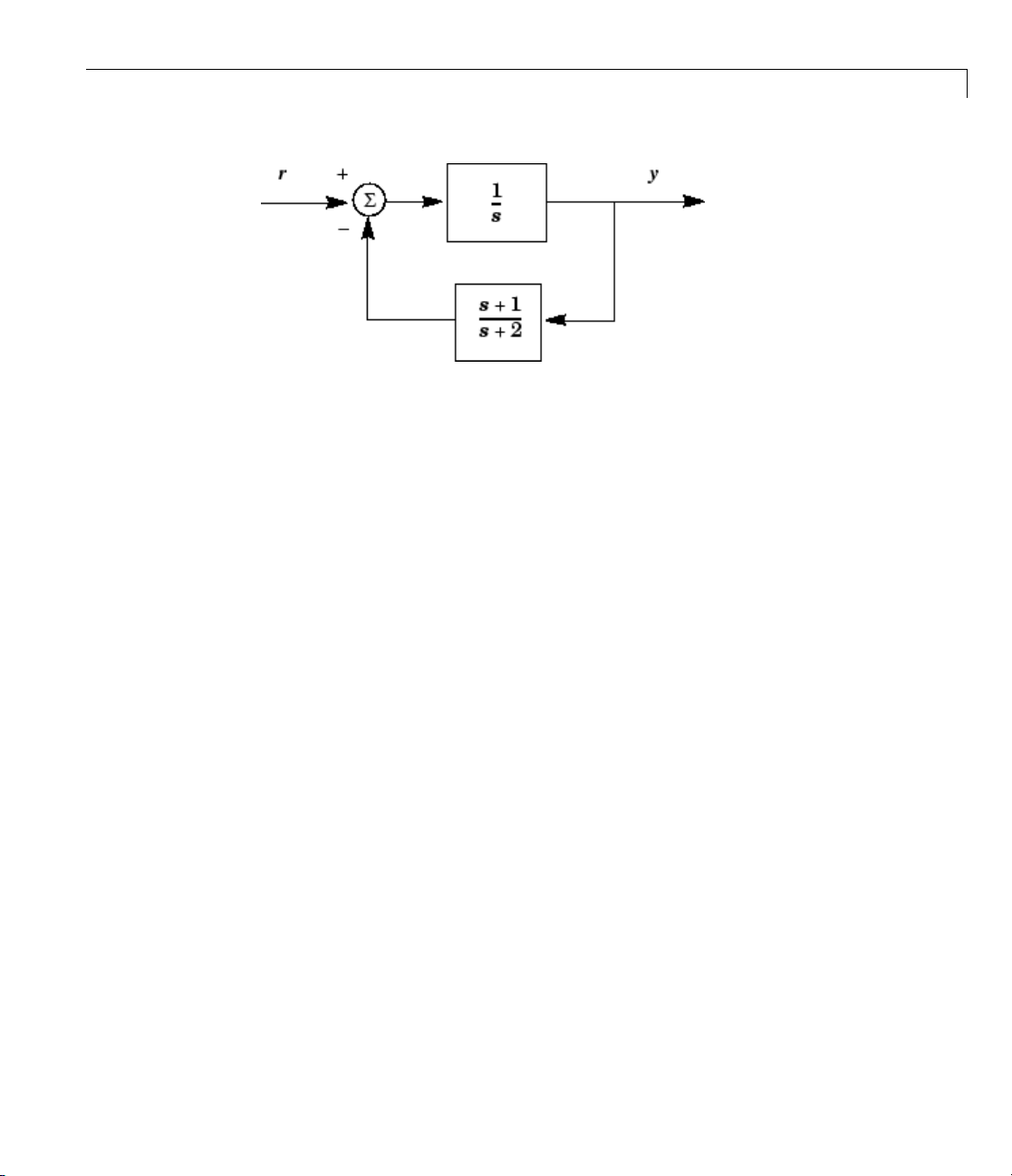
Interconnecting Linear Models

Feedback Interconnection

You can use the lft function to create more complicated feedback structures. This function constructs the linear fractional transformation of two systems. See the reference page for more information.

2-25

2 Building Models

Converting Between Continuous- and Discrete- Time Systems

In this section...

“Available Commands for Continuous/Discrete Conversion” on page 2-26

“Available Methods for Continuous/Discrete Conversion” on page 2-26

“Digitizing the Discrete DC Motor Model” on page 2-26

Available C Conversio

The comman continuou

sysd = c2d(sysc,Ts) % Discretization w/ sample period Ts sysc = d2c(sysd) % Equivalent continuous -time model sysd1= d2d( sysd,Ts) % Resampling at the period Ts

s, and discrete to discrete (resampling) conversions, respectively.

Available Met

ommands for Continuous/Discrete

c2d, d2c,andd2d perform continuous to discrete, discrete to

hods for Continuous/Discrete

Conversion

Various discr zero-order h without prew

sysd = c2d(sysc,Ts,'f oh') % Uses first-order hold sysc = d2c(sysd,'tusti n') % Uses Tustin approximation

Digitizing the Di

You can digitize appropriate sam factors, includ constant in your to run. For this Example: The DC

sys_dc.

etization/interpolation methods are available, including

old (default), first-order hold, Tustin approximatio n with or

arping, and matched zero-pole. For ex ample,

screte DC Motor Model

the DC motor plant using the ple time. Choosing the rig ht sample time involves many

ing the performance you want to achieve, the fastest time

system, and the spe ed at which you expect your controller

example, choose a time constant of 0.01 second. See “SISO

Motor” on page 2-3 for the cons truction of the SS object

c2d function and selecting an

2-26

Ts=0.01;

sysd=c2d(sys_dc,Ts)

x1 0.96079 -0.00027976 x2 0.006994 0.90484

x1 0.019605 x2 7.1595e-005

y101

Converting Between Continuous- and Discrete- Time Systems

x1 x2

y1 0

Sampling ti me: 0.01 Discrete-time model.

To see the discrete-time zero-pole gain for the digital DC motor, use zpk to convert the model.

fd=zpk(sysd)

Zero/pole/gain:

7.1595e-005 (z+0.9544)

------------------------

(z-0.9608) (z-0.9049)

Sampling ti me: 0.01

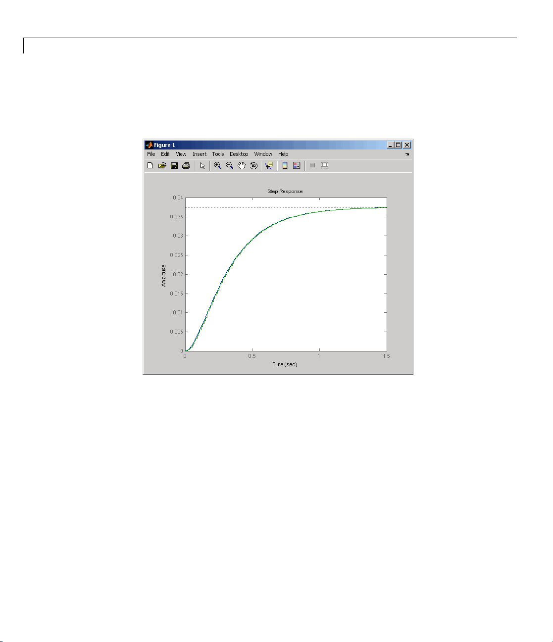
You can compare the step responses of sys_dc and sysd by typing

2-27

2 Buildin g Models

step(sys_dc,sysd)

This figure shows the result.

2-28

Note the s t ep response match. C ontinuous and FOH-discretized step responses match for models without internal delays.

Reducing Model Order

In this section...

“Model Order Reduction Commands” o n page 2-29

“Techniques for Reducing Model Order” on page 2-29

“Example: Gasifier Model” on page 2-30

Model Order Reduction Commands

You can derive reduced-order SISO and MIMO models with the commands shown in the following table.

Model Order Reduction Commands

hsvd

balred

minreal

balreal

modred

sminreal

Reducing Model Order

Compute Hankel singular values of LTI model

Reduced-order model approximation

Minimal realization (pole/zero cancellation)

Compute input/output balanced realization

State deletion in I/O balanced realization

Structurally minimal realization

hniques for Reducing Model Order

Tec

educe the order of a model, you can perform any of the following actions:

To r

iminate states that are structurally disconnected from the inputs or

• El

tputs using

iminating structurally disconnected states is a good first step in model

duction because the process is cheap and does not involve any numerical

omputation.

ompute a low-order approximation of your model using

• C

liminate cancelling pole/zero pairs using

• E

sminreal.

balred.

minreal.

2-29

2 Buildin g Models

Example: Gasifier Model

This example presents a model of a gasifier, a device that converts solid materials into gases. The original m odel is nonlinear.

Loading the Model

To load a linearized version of the model, type

load ltiex amples

at the MATLAB prompt; the gasifier example is stored in the variable named

gasf.Ifyoutype

size(gasf)

you get in return

State-space model wit h 4 outputs, 6 inputs, and 25 states.

2-30

SISO Model Order Reduction

You can reduce the order of a single I/O pair to understand how the model reduction tools work before attempting to reduce the full MIMO model as described in “MIMO Model Order Reduction” on page 2-34.

This example focuses on a single input/output pair of the gasifier, input to output 3.

sys35 = gasf(3,5);

Before attempting model order reduction, inspect the pole and zero locations by typing

pzmap(sys35)

Zoom in near the origin on the resulting plo t using the zoom feature or by typing

axis([-0.2 0.05 -0.2 0.2])

The following figure shows the results.

Reducing Model Order

Pole-Zer

Because for mode

To find

1 Select

o Map of the Gasifier Model (Zoomed In)

the m odel displays near pole-zero cancellations, it is a good candidate l reduction.

a low-order reduction of this SISO model, perform the following steps:

an appropriate orde r for your reduced system by examining the

ve amount of energy per state using a Hankel singular value (HSV)

relati

Type the command

plot.

hsvd(sys35)

eate the HSV plot.

to cr

Changing to log scale using the right-click menu results in the following plot.

2-31

2 Buildin g Models

2-32

Small Hankel singular values indicate that the associated states contribute little to the I/O behavior. This plot shows that discarding the last 10 states (associated with the 10 sma llest Hankel singular values) has little impact on the approximation error.

2 To remove the last 10 states and create a 15th order approximation, type

rsys35

= balred(sy s35,15);

You can type s ize (rsys35) to see that your reduced system contains only 15 states.

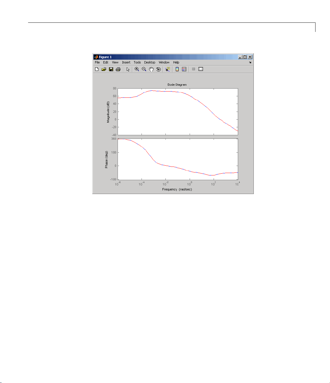
3 Comp

are the Bode response of the full-order and reduced-order models

g the bode command:

usin

bode(sys35,'b',rsys35,'r--')

s figure shows the result.

Thi

Reducing Model Order

As the overlap of the curves in the figure shows, the reduced m odel provides a good approximation of the original system.

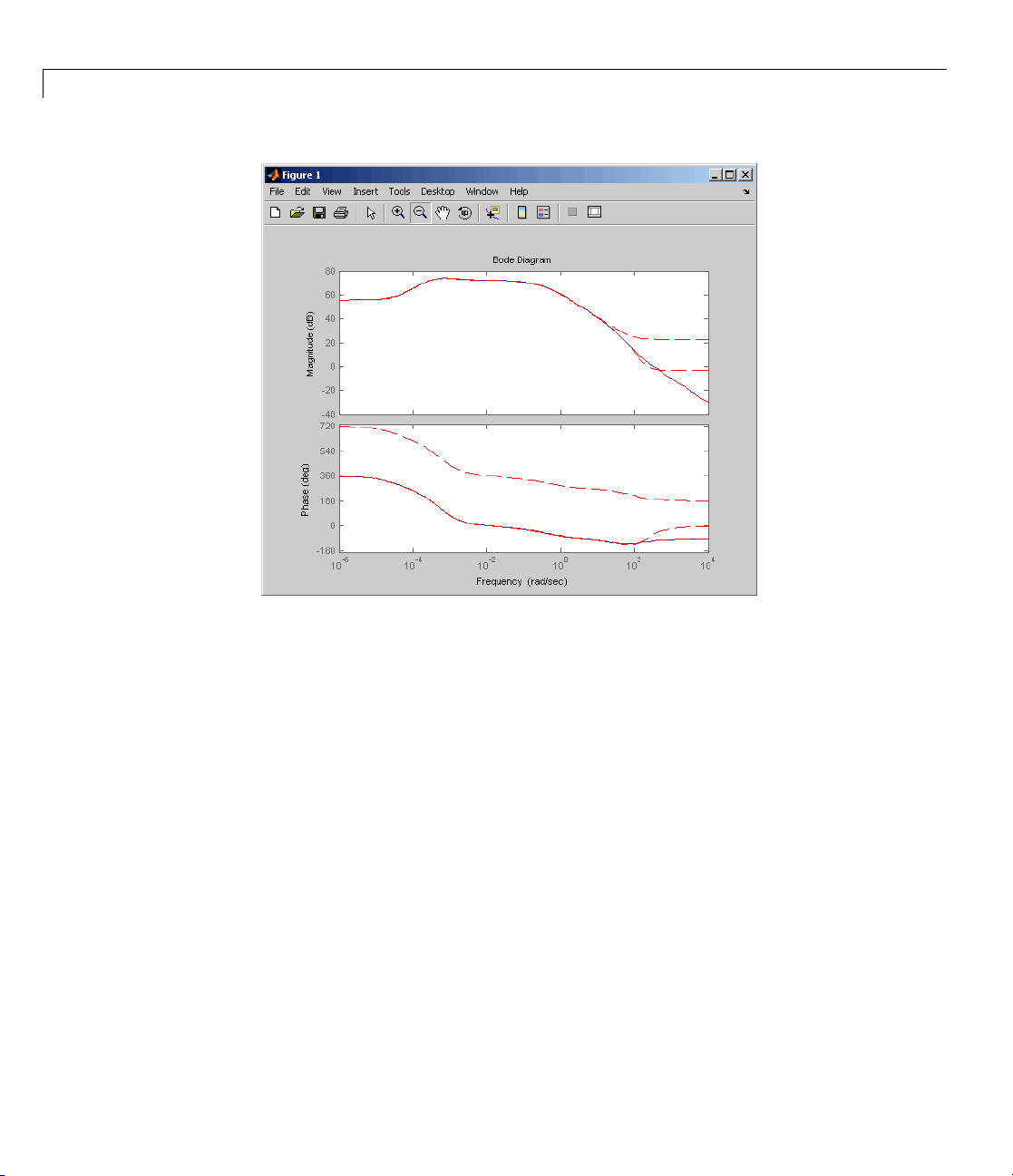
You can try reducing the model order further by repeating this process and removing more states. Reduce the

gasf model to 5th, 10th, and 15th orders

allatoncebytypingthefollowingcommand

rsys35 = balred(sys35 ,[5 10 15]);

Plot a bode diagram of these three reduced syste ms along with the full order system by typing

bode(sys35,'b',rsys35,'r--')

2-33

2 Buildin g Models

2-34

Observe h

ow the error increases as the order decreases.

MIMO Model Order Reduction

You can a follow

1 Select

relati plot.

Type

to create the HSV plot.

pproximate MIMO models using the same steps as SISO models as

an appropriate orde r for your reduced system by examining the

ve amount of energy per state using a Hankel singular value (HSV)

hsvd(gasf)

Reducing Model Order

Discarding the last 8 states (associat ed with the 8 smallest Hankel singular values) should have little impact on the error in the resulting 17th order system.

2 To remove the last 8 states and create a 17th order MIMO system, type

rsys=b

alred(gasf,17);

You can type size(gasf) to see that your reduced system contains only 17 states.

3 To fac

ilitate visual inspection of the approximation error, use a singular

e plot rather than a MIMO Bode plot. Type

valu

sigma(gasf,'b',gasf-rsys,'r')

reateasingularvalueplotcomparingtheoriginalsystemtothe

to c

uction error.

red

2-35

2 Buildin g Models

2-36

The reduction e rror is small compared to the original system so the reduced order model provides a good approximation of the original model.

Acknowledgment

MathWorks thanks ALSTOM®Power UK for permitting use of their gasifier model for this example. This model was issued as part of the ALSTOM Benchmark Challenge on Gasifier Control. For more details see Dixon, R., (1999), "Advanced Gasifier Control," Computing & Control Engineering Journal, IEE, Vol. 10, No. 3, pp. 92–96.

Analyzing Models

• “Quick Start for Performing Linear Analysis Using the LTI Viewer” on

page 3-2

• “LTI Viewer” on page 3-7

• “Simulating Models with Arbitrary Inputs and Initial Conditions” on page

3-22

• “Functions for Time and Frequency Response” on page 3-37

3 Analyzing Models

Quick Start for Performing Linear Analysis Using the LTI Viewer

In this Quick Start, you learn how to analyze the time- and frequency-d omain responses of one or more linear models using the LTI Viewer GUI.

Before you can perform the analysis, you must have already created linear models in the MATLAB workspace. For information on how to create a model, see Chapter 2, “Building Models”.

To perform linear analysis:

1 Open the LTI Viewer showing one or more models using the following

syntax:

ltiview(model1,model2,...,modelN)

By default, this syntax opens a step response plot of your models, as shown in the following figure.

3-2

Quick Start for Performing Linear Ana lysi s Using the LTI Viewer

Click to add a legend

3-3

3 Analyzing Models

2 Add more plots to the LTI Viewer.

a Select Edit > Plot Configurations.

b In the Plot Configurations dialog box, select the number of plots to open.

3-4

Select the number of plots to open

Quick Start for Performing Linear Ana lysi s Using the LTI Viewer

3 To view a different type of response on a plot, right-click and select a plot

type.

Right-click to select a plot type

3-5

3 Analyzing Models

4 Analyze system performance. For example, you can analyze the peak

response in the Bode plot and settling time in the step response plot.

a Right-click to select performance characteristics.

b Click on the dot that appears to view the characteristic value.

Right-click to show performance characteristics

Click dot to view value

3-6

LTI Viewer

LTI Viewe r

In this section...

“Plot Types Available in the LTI Viewer” on page 3-7

“Example: Time and Frequency Responses of the DC Motor” on page 3-8

“Right-Click Menus” on page 3-10

“Displaying Response Characteristics on a Plot” on page 3-11

“Changing Plot Type” on page 3-14

“Showing Multiple Response Types” on page 3-16

“Comparing Multipl e Models” on page 3-17

Plot Types Available in the LTI Viewer

The LTI Viewer is a GUI for vie wing and manipulating the response plots of linear models. You can display the following plot types for linear models using the LTI Viewer:

• Step and impulse responses

• Bode and Nyquist plots

• Nichols plots

• Singular values of the frequency response

• Pole/zero plots

• Response to a general input signal

• Unforced response starting from given initial states (only for state-space

models)

Note that time responses and pole/zero plots are not available for FRD models.

Note The LTI Viewer displays up to six different plot types simultaneously. You can also analyze the response plots of several linear models at once.

3-7

3 Analyzing Models

This figure shows an LTI Viewer with two response plots.

The LTI Viewer with Step and Impulse Response Plots

The next section presents an example that shows you how to import a system into the LT I Viewer and how to customize the viewer to fit your requirements.

Example: Time and Frequency Responses of the DC Motor

“SISO Example: The DC Motor” on page 2-3 presents a DC motor example. If you have not yet built that example, type

ltiexamples

load

at the MATLAB prompt. This loads several LTI models, including a state-space representation of the DC motor called

3-8

sys_dc.

LTI Viewe r

Opening the LTI Viewer

To open the LTI Viewer, type

ltiview

This opens an LTI Viewer with an empty step response plot window by default.

Importing Models into the LTI Viewer

To import the DC motor model, select Import under the File m enu. This opens the Import System Data dialog box, which lists all the models available in your MATLAB workspace.

Import System Data Dialog Box w ith the DC Motor M od el Selected

Select sys_dc from the list of available models and click OK to close the browser. This im po rts the DC motor model into the LTI Viewer.

To select more than one model at a time, do the follow ing:

• To select individual (noncontiguous) models, select one model and hold

down the Ctrl key while selecting additional models. To clear any models, hold down the Ctrl k ey while you click the highlighted model nam es.

• To select a list of contiguous models, select the first mode l and hold down

the Shift key while selecting the last model you want in the list.

3-9

3 Analyzing Models

The figure below shows the LTI Viewer with a step response for the DC motor example.

3-10

Step Response for the DC Motor Example in the LTI Viewer

Alternatively, you can open the L TI Viewer and import the DC mo to r example directly from the MATLAB prompt.

ltiview('step', sys_dc)

See the ltiview reference page for a complete list of options.

Right-Click Menus

The LTI Viewer provides a set of controls and options that you can access by right-clicking your mouse. Once you have imported a model into the LTI Viewer, the options you can select include

• Plot Types — Change the plot type. Available types include step, impulse,

Bode,Bodemagnitude,Nichols,Nyquist,andsingularvaluesplots.

• Systems — Select or clear any models that you included when you created

theresponseplot.

• Characteristics — Add information about the plot. The characteristics

available change from plot to plot. For example, Bode plots have stability margins available, but step responses have rise time and steady-state values available.

• Grid —Addgridstoyourplots.

• Normalize — Scale responses to fit the view (only available for

time-domain plot types).

• Full View — Use automatic limits to make the entire curve visible.

• Properties — Open the Property Editor.

LTI Viewe r

You can use this editor to customize various attributes of your plot. See Customizing Plot Properties and Preferences for a full description of the Property Editor.

Alternatively, you can open the Property Editor by double-clicking in an empty region of the response plot.

Displaying Response Characteristics on a Plot

Forexample,toseetherisetimeforthe DC m otor step response, right-click and select Characteristics > Rise Time.

3-11

3 Analyzing Models

3-12

Using Rig

By defau respons range in proper

The LTI

e to go from 10% to 90% of the steady-state value. You can change this

ty editor, see Customizing Plot Properties and Pre ferences.

ht-Click Menus to Display the Rise Time for a Step Response

lt, the rise time is defined as the amount of time it takes the step

the options tab of the property editor. For more information on the

Viewer calculates and displays the rise time for the step response.

LTI Viewe r

DC Motor S

To displ your mou

data mar

persis

For exa respon

tep Response with the Rise Time Displayed

ay the values of any plot characteristic marked on a plot, place

se on the blue dot that marks the characteristic. This opens a

ker with the relevant information displayed. To make the marker

tent, left-click the blue dot.

mple, this figure shows the rise time value for the DC motor step

se.

3-13

3 Analyzing Models

3-14

Using You

Note tha respons over the

For mor

Chang

You ca examp sele

r Mouse to Get th e Rise Time Values

t you can left-click anyw here on a particular plot line to see the

e values of that plot at that point. You must either place y our cursor

bluedotorleft-click,however,ifyouwanttoseetherisetimevalue.

e information about data markers, see “Data Markers” on page 3-42.

ing Plot Type

n view other plots using the right-click menus in the LTI Viewer. For le, if you want to see the open loop Bode plots for the DC motor model,

ct Plot Type and then Bode from the right-click menu.

LTI Viewe r

Changing

Selecti

ng Bode changes the step response to a Bode plot for the DC motor

model.

the Step Response to a Bode Plot

3-15

3 Analyzing Models

3-16

Bode Plot

for the DC Motor Model

Showing

If you wa the sam respon Edit me

nt to see, for example, both a step response and a Bode plot at

e time, you have to reconfig ure the LTI View er. To view different

se types in a single LTI Viewer, select Plot Configurations under the

nu. This opens the Plot Configurations dialog box.

Multiple Response Types

Using the Plot Configurations Dialog Box to Reco nfigure the LTI Viewer

You can select up to six plots in one viewer. Choose the R esponse type for each plot area from the right-side menus. There are nine available plot types:

• Step

LTI Viewe r

• Impulse

• Linear Simulation

• Initial Condition

• Bode (magnitude and phase)

• Bode Magnitude (only)

• Nyquist

• Nichols

• Singular Value

• Pole/Zero

• I/O pole/zero

Comparing Multiple Models

This section shows you how to import and manipulate multiple models in one LTI Viewer. For example, if you h ave designed a set of compensators to control a system, you can compare the closed-loop step responses and Bode plots using the LTI Viewer.

3-17

3 Analyzing Models

A sample set of clo sed-loo p transfer function models is included (along with some other models) in the MAT-file

load ltiex amples

to load the provided transfer functions. The three closed-loop transfer function models,

Gcl1, Gcl2,andGcl3, are for a satellite attitude controller.

ltiexamples.mat.Type

In this example, you analyze the response plots of the functions.

Gcl1 and Gcl2 transfer

Initializing the LTI Viewer with Multiple Plots

To load the two models Gcl1 and Gcl2 into the LTI Viewer, select Import under the File menu and select the desired models in the LTI Browser. See “Importing Models into the LTI Viewer” on page 3-9 for a description of how to select groups of models. If necessary, you can reconfigure the viewer to display both the step responses and the Bode plots of the two systems using the Viewer Configuration dialog box. See“ShowingMultipleResponseTypes” on page 3-16 for a discussion of this feature.

Alternatively, you can open an LTI Viewer with both systems and both the step responses and Bode plots displayed. To do this, type

ltiview({'step';'bode'},Gcl1,Gcl2)

Either approach opens the following LTI Viewer.

3-18

LTI Viewe r

Multiple

Response Plots in a Single LTI Viewer

Inspecting Response Characteristics

To mark t do the f

• Right-

opens t

• Selec

To mar sele

Your

he settling time on the step responses presented in this example,

ollowing:

click anywhere in the plot region of the step response plots. This

he right-click menu list in the plot region.

t Characteristics > Settling Time.

k the stability margins of the Bode plot in this example, right-click and

ct Characteristics > Minimum Stability Margins.

LTI Viewer should now look like this.

3-19

3 Analyzing Models

3-20

Multiple

The mini gain mar diagram right-

Plots with Response Characteristics Added

mum stability margins, meaning the smallest magnitude phase and gins, are displayed as green and blue markers on the Bode phase

. Ifyouwanttoseeallthegainandphasemarginsofasystem,

click and select Characteristics > Minimum Stability Margins.

Toggling Model Visibility

have imported more than one model, you can s elect and clear which

If you

s to plot in the LTI Viewer using right-click menus. For example, if you

model

t the following three models into the viewer, you can choose to view any

impor

ination of the three you want.

comb

s=tf('s'); sys1=1/(s^2+s+1); sys2=1/(s^2+s+2); sys3=1/(s^2+s+3);

LTI Viewe r

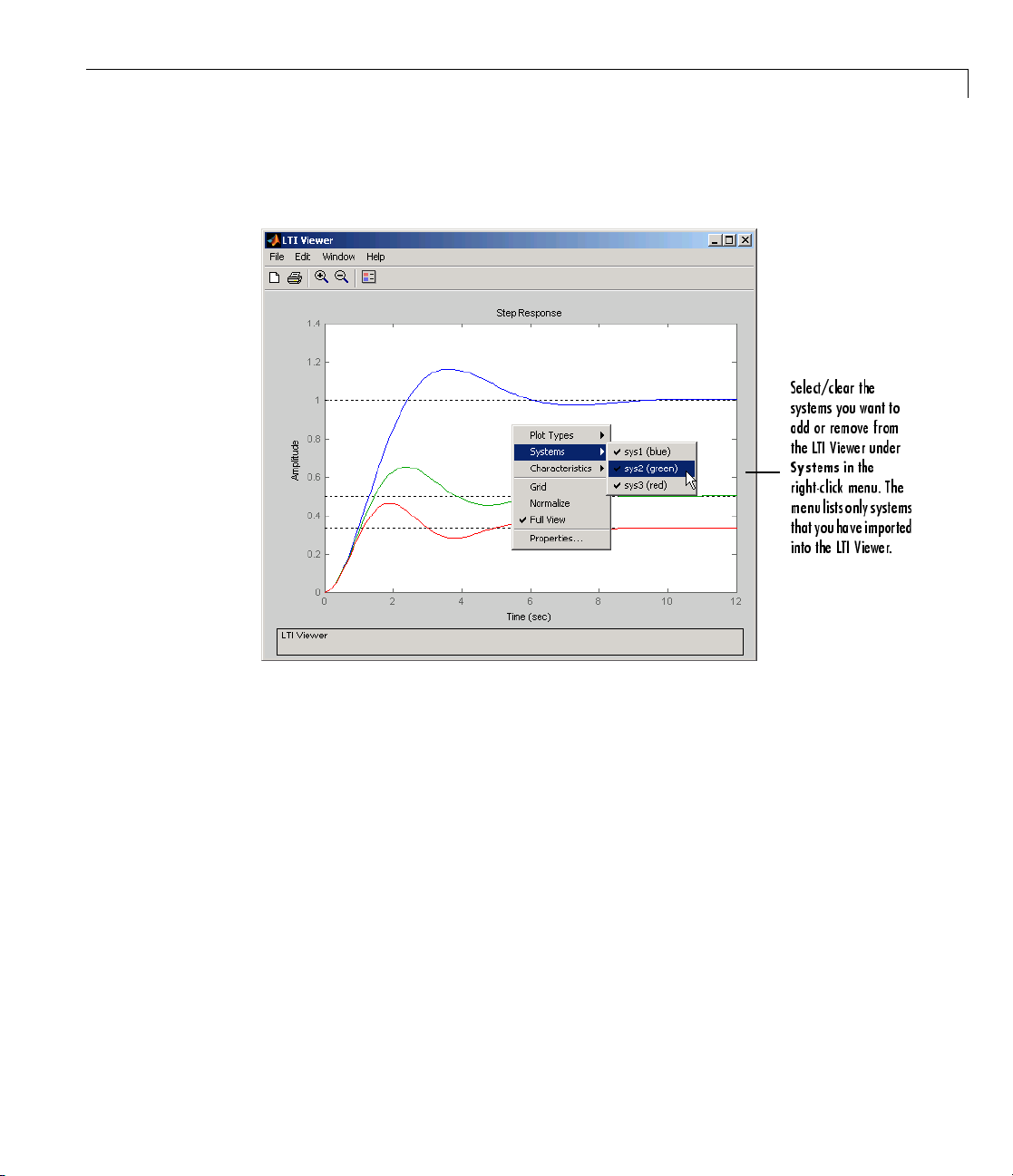
This figure shows how to clear the second of the three models using right-click menu options.

Using Right-Click Menus to Select/Clear Plotted Systems

The Systems menu lists all the imported models. A system is selected if a check mark is visible to the left of the system name.

3-21

3 Analyzing Models

Simulating Models with Arbitrary Inputs and Initial Conditions

In this section...

“What is the Linear Simulation Tool?” on page 3-22

“Opening the Linear Simulation Tool” on page 3-22

“Working with the Linear Simulation Tool” on page 3-23

“Importing Input Signals” on page 3-26

“Example: Loading Inputs from a M icrosoft®Excel Spreadsheet” on page 3-28

“Example: Importing Inputs from the W orkspace” on page 3-29

“Designing Input Signals” on page 3-33

“Specifying Initial Conditions” on page 3-35

3-22

What is

You can

rary input s i gn als and ini tia l conditions.

arbit

The Li

• Impo

ASC

• Gen

pfunction,orwhitenoise.

ste

ecify initial states for state-space models.

• Sp

fault initial states are zero.

pening the Linear Simulation Tool

o open the Linear Simulation Tool, do one of the following:

the Linear Simulation Tool?

use the Linear Simulation Tool to simulate linear models with

near Simulation Tool lets you do the following:

rt input signals from the MATLA B workspace.

rt input signals from a MAT-file, Microsoft

II flat-file, comma-separated variable file (CSV), or text file.

erate arbitrary input signals in theformofasinewave,squarewave,

Excel®spreadsheet,

Simulating Models with Arbitrary Inputs and Initial Conditions

• In the LTI Viewer, right-click the plot area and select Plot Types >

Linear Simulation.

• Use the

lsim function at the MATLAB prompt:

lsim(modelname)

• IntheMATLABFigurewindow,right-click a response plot and select

Input data .

Working with the Linear Simulation Tool

The Linear Simulation Tool contains two tabs, Input signals and Initial states.

After opening the Linear Simulation Tool (as described in “Opening the Linear Simulation Tool” on page 3-22), follow these steps to simulate your model:

1 Click the Input signals tab, if it is not displayed.

3-23

3 Analyzing Models

2 In the Timing area, specify the simulation time vector by doing one of

the following:

• Import the time vector by clicking Import time.

• Enter the end time and the time interval in s econds. The start time

is set to

3 Specify the input signal by doing one of the following:

0 seconds.

• Click Import signal to import it from the MATLAB workspace or a file.

For more information, see “Importing Input Signals” on page 3-26.

• Click Design signal to create your ow n inputs. For more information,

see “Designing Input Signals” on page 3-33.

4 If you have a state-space model and want to specify init ial conditions, click

the Initial states tab. By default, all initial states are set to zero.

You can either enter state values in the Initial value column, or import values by clicking Import state vector. For more information about entering initial states, see “Specif yi n g In iti al Conditions” on page 3-35.

3-24

Simulating Models with Arbitrary Inputs and Initial Conditions

5 For a con

the Inte

• Zero or

• First o

• Autom

hold a

Note

mode

ck Simulate.

6 Cli

tinuous model, select one of the following interpolation methods in

rpolation method list to be used by the simulation solver:

der hold

rder hold (linear interpolation)

atic (Linear Simulation Tool selects first order hold or zero order

utomatically, based on the smoothness of the input)

The interpolation method is not used when simulating discrete

ls.

3-25

3 Analyzing Models

Importing Input

You can import in the Linear Simul page 3-22). You ca spreadsheet, A

For informati Signals” on pa Tool, see “Wo

To import one

1 In the Linea

displayed.

2 Specify the simulation time in the Timing area.

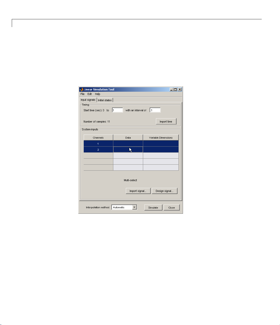
3 Select one or mo re rows for the input channels you want to import. The

following figure shows an example with two selected channels.

ation Tool (see “Opening the Linear Simulation Tool” on

SCII flat-file, comma-separated variable file (CSV), or text file.

on about creating your own inputs, see “D esigning Input

ge 3-33. For an overview of w ork ing with the Linear Simulation

rking with the Line ar Simulation Tool” on page 3-23.

or more input signals:

r Simulation Tool, click the Input signals tab, if it is not

Signals

put signals from the MATLAB workspace after opening

n also import inputs from a MAT-file, Microsoft Excel

3-26

Simulating Models with Arbitrary Inputs and Initial Conditions

4 Click Import signal to open the Data Import dialog box. The following

figure shows an example of the Data Import dialog box.

3-27

3 Analyzing Models

5 In the Import from list, select the source of the input signals. It can be

one of the following:

•

Workspace

• MAT file

• XLS file

• CSV file

• ASCII file

6 Select the data you want to import. The Data Import dialog box contains

different options depending on which source format you selected.

7 Click Import.

For an example of importing input signals, see the foll owing:

• “Example: Loading Inputs from a Microsoft

Excel Spreadsheet” on p ag e

3-28

• “Example: Importing Inputs from the Workspace” on page 3-29

Example: Loading Inputs from a Microsoft Excel Spreadsheet

To load inputs from a Microsoft Excel (XLS) spreadsheet:

1 In the Linear Simu lation Tool, click Impo r t signal in the Input signals

tab to ope n the Data Import dialog box .

2 Select XLS file in th e Import from list.

3 Click Browse.

4 Select the file you want to import and click Open. This populates the Data

Import dialog box with the data from the Microsoft Excel spreadsheet.

3-28

Simulating Models with Arbitrary Inputs and Initial Conditions

Example: Importing Inputs from the Workspace

To load an input signal from the M ATLAB workspace:

1 Enter this code to open a response plot with a second-order system:

s=tf('s'); ss=(s+2)/(s^2+3*s+2); lsim(ss,randn(100,1),1:100);

2 Right-click the plot background and select Input data.

3-29

3 Analyzing Models

3-30

This opens the Linear Simulation Tool with default input data.

Simulating Models with Arbitrary Inputs and Initial Conditions

3 Create an input signal for your system in the MATLAB Command Window,

such as the following:

new_signal=[-3*ones(1,20) 2*ones(1,30) 0.5*ones(1,50)]';

4 In the Linear Simulation Tool, click Import signal.

5 In the Data Imp ort dialog box, click, Assign columns to assign the first

column of the input signal to the selected channel.

3-31

3 Analyzing Models

6 Click Import. This imports the new signal into the Linear Simulation Tool.

3-32

Simulating Models with Arbitrary Inputs and Initial Conditions

7 Click Simulate to see the response of your second-order system to the

imported signal.

Designing Input Signals

You can generate arbitrary input signals in the form of a sine wave, square wave, step function, or white noise after opening the Linear Simulation Tool (see “Opening the Linear Simulation Tool” on page 3-22).

For information about importing inputs from the MATLAB workspace or from a file, see “Importing Input Signals” on page 3-26. For an overview of working with the Linear Simulation Tool, see “W orking with the Linear Simulation Tool” on page 3-23.

To design one or more input signals:

1 In the Linear Simulation Tool, click the Input signals tab (if it is not

displayed).

3-33

3 Analyzing Models

2 Specify the simulation time in the Timing area. The time interval (in

seconds) is used to evaluate the input signal you design in later steps of this procedure.

3 Select one or more rows for the signal channels you want to design. The

following figure shows an example with two selected channels.

3-34

4 Click Design signal to open the Signal Designer dialog box. The following

figure shows an example of the Signal Designer dialog b ox.

Simulating Models with Arbitrary Inputs and Initial Conditions

5 In the Signa

can be one o

•

Sine wav e

• Square wa

• Step func

• White no

6 Specify the signal characteristics. The Signal Designer dialog box contains

ltypelist, select the type of signal you want to create. It

f the following:

tion

ise

different options depending on which signal type you selected.

7 Click Insert. This brings the new signal into the Linear Simulation Tool.

8 Click S

Speci

If you afte Tool

For a wit

You

imulate in the Linear Sim u la t ion T o o l to view th e system response.

fying In itial Conditions

r system is in state-space form, you can enter or import initial states

r opening the Linear Simulation Tool (see “Opening the Linear Simulation

”onpage3-22).

n overview of working with the Linear Simulation Tool, see “Working

h the Linear Simulation Tool” on page 3-23.

can also import initial states from the MATLAB workspace.

3-35

3 Analyzing Models

To import one or more initial states:

1 In the Linear Sim ulation Tool, click the Initial s tates tab (if it is not

already displayed).

2 In the Selected system list, select the system for which you want to

specify initial conditions.

3 You can either enter state values in the Initial value column, or import

values from the MATLAB workspace by clicking Import state vector. The following figure shows an example of the import window:

3-36

Note For

4 After s

Tool to

n-states, your initial-condition vector must have n entries.

pecifying the initial states, click Simulate in the Linear Simulation

view the system response.

Functions for Time and Frequency Response

In this section...

“When to Use Functions for Time and Frequency Response” on page 3-37

“Time and Frequency Response Functions” on page 3-37

“Plotting MIMO M odel Responses” on page 3-40

“Data Markers” on page 3-42

“Plotting and Comparing Multiple Systems” on page 3-44

“Creating Custom Plots” on page 3-47

When to Use Functions for Time and Frequency Response

You can use the LTI Viewer GUI for a wide range of applications. There are situations, however, where you may want a more open and extensible environment. You can use the Control System Toolbox functions for basic time and frequency domain analysis plots used in control system engineering. These functions apply to any kind of linear model (continuous or discrete, SISO or MIMO, or arrays of models). Yo u can o nly apply the frequency domain analysis functions to FRD models.

Use the LTI Viewer when a GUI-driven environment is desirable. On the other hand, use functions when you want customized plots. If you want to include data unrelated to your models, you must use functions instead of the LTI Viewer (which only plots model data).

The next sections discuss time and frequency response functions and how to use these functions to create customized plots of linear model responses.

Time and Frequency Response Functions

Time responses investigate the time-domain transient behavior of linear modelsforparticularclassesofinputs and disturbances. You can determine such system characteristics as rise time, settling time, overshoot, and steady-state error from the time response. You can use the Control System Toolbox functions for step response, impulse response, initial condition

3-37

3 Analyzing Models

response, and general linear simulations. For example, you can simulate the response to white noise inputs using

lsim and the MATLAB function randn.

In addition to time-domain analysis, you can use the Control System Toolbox functions for frequency-domain analysis using the following standard plots:

• Bode

• Nichols

• Nyquist

• Singular value

This table lists available time and frequency response functions and their use.

Functions for Frequency and Time Response

Functions Description

bode

evalfr

Bode plot

Computes the frequency response at a single complex frequency (not for FRD models)

freqresp

Computes the frequency response for a set of frequencies

gensig

impulse

initial

iopzmap

lsim

margin

nichols

nyquist

pzmap

step

Input signal generator (for lsim)

Impulseresponseplot

Initial condition response plot

Pole-zero map for each I/O pair of an LTI model

Simulation of response to arbitrary inputs

Computes and plots gain and phase margins

Nichols plot

Nyquist plot

Pole-zero map

Step response plot

3-38

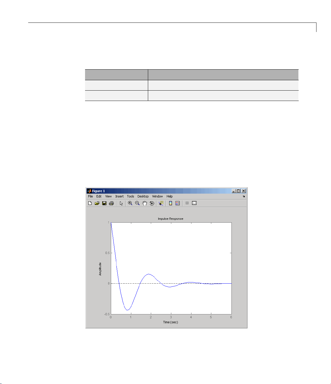
Functions for Time and Frequency Response

Functions for Frequency and Time Response (Continued)

Functions Description

hsvd

bodemag

Compute Hankel singular values of LTI model

Bode magnitude response of LTI models

ThesefunctionscanbeappliedtosinglelinearmodelsorLTIarrays.

The functions

step, impulse,andinitial automatically generate an

appropriate simulation horizon for the time response plots. For example,

h = tf([1 0],[1 2 10]) impulse(h)

produces the following plot.

Impulse Response of a SISO Model

3-39

3 Analyzing Models

Frequency-domain plots automatically generate an appropriate frequency range as well.

Plotting MIMO Model Responses

For MIMO models, time and frequency response functions produce an array of plots with one plot per I/O channel (or per output for For example,

h = [tf(10,[1 2 10]) , tf (1,[1 1])] step(h)

produces the following plot.

initial and lsim).

3-40

Step Responses for a MIMO Model

The simulation horizon is automatically determined based on the model dynamics. You can override this automatic mode by specifying a final time,

ep(h,10) % Simulates from 0 to 10 seco nds

Functions for Time and Frequency Response

or a vector of evenly spaced time samples.

t = 0:0.01:10 % Time samples spaced every 0.01 second step(h,t)

Right-Click Menus

All the time and frequency response functions provide right-click menus that allow you to customize your plots. For more information on using the LTI Viewer right-click menus, see “Using the Right-Click Menu in the LTI Viewer”. This figure shows the plots from Step Responses for a MIMO Model on page 3-40, with the right-click menu open.

Using the Right-Click Menu in a Step Re spon se Plot

The options you can select include

3-41

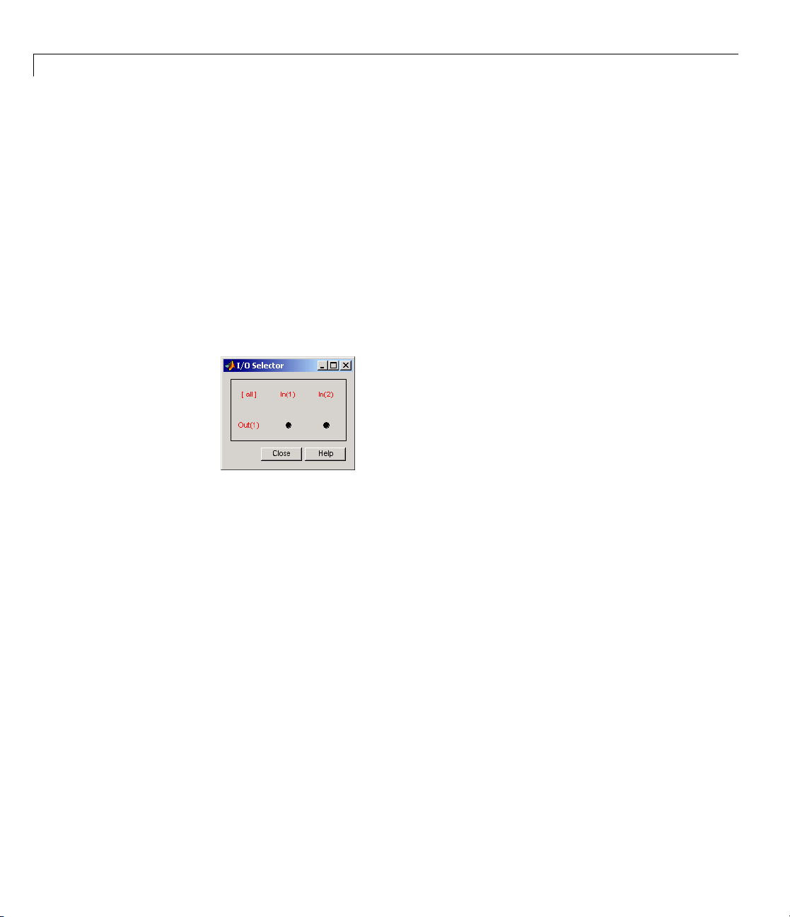
3 Analyzing Models

• Systems — Select or clear any models that you included when you created

theresponseplot.

• Characteristics — Add information about the plot. The characteristics

available change from plot to plot. For example, Bode plots have stability margins available, but step responses have rise time and steady-state values available.

• Axes Grouping — Change the grouping of your plots. Available options

are All, None, Inputs, and Outputs. You can group all the plots together, placeeachinaseparateplotregion(none), or group the inputs or outputs together.

• I/O Selector —OpentheI/O Selector dialog box.

3-42

Use this dialog box to select/clear which inputs and outputs to plot.

• Normalize — Scale responses to fit the view (only available for

time-domain plot types).

• Full View — Use automatic limits to make the entire curve visible.

• Grid —Addgridstoyourplots.

• Properties — Open the Property Editor, which you can use to customize

various attributes of your plot. See Customization for a full description of the Property Editor.

Alternatively, you can open the Property Editor by double-clicking in an empty region of the response plot.

Data Markers

In addition to right-click menus, you can use plot data markers. These allow you to identify key data points on your plots. This figure, using the s ame plot as Step Responses for a MIMO M odel on page 3-40, shows markers on the plots.

Functions for Time and Frequency Response

Using Plo

You can m

• Grabbi

• Draggi

The ti does n rise t by pla To ma

Note

dat Des

t Ma r kers to Identify Data Points

ove a data marker by

ng the black square located at the corner of the marker

ngthemarkerwithyourmouse

me and am plitude values will change as you move the marker. This

ot apply to markers that display plot characteristics (e.g., peak value or

ime). In the case of plot characteristic data markers, you can view them

cing your cursor over the dot that represents the active characteristic.

ke the data marker persistent, left-click the marker.

Data markers do not apply to the SISO Design Tool, which displays

a about plot characteristics in the status pane at the bottom o f the SISO

ign Tool window.

3-43

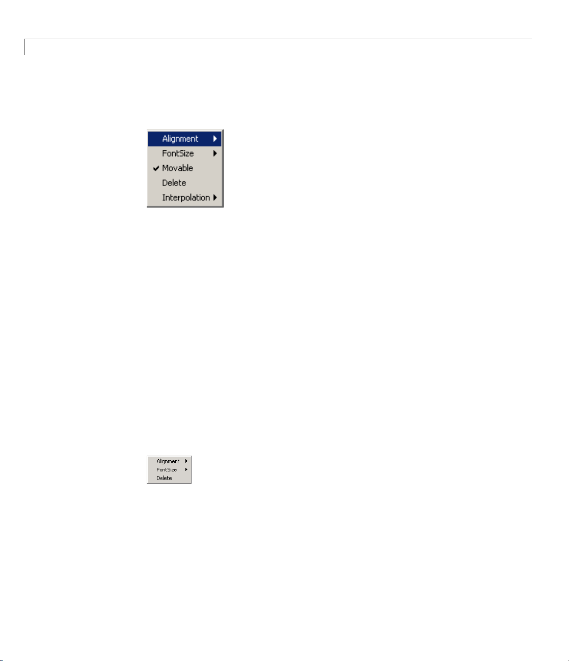
3 Analyzing Models

Right-Click Menus

Right-click on any data marker to open a property menu for the marker.

Property options for the marker include

• Alignment — Change the position of the marker. Available options are

top-right, top-left, bottom-right, and bottom-left.

• FontSize — Change the font size.

• Movable — By default, you can move data markers by clicking and

dragging. Clearing Movable forces the marker to remain at a f ixed data point.

3-44

• Delete — Remove the sele cte d marker. Alternati vely, left-click anywher e

in the empty plot region to delete all markers in the plot

• Interpolation — By default, data m arkers linearly interpolate between

points along the plotted curve. Select None to force the markers to snap to nearest points along the plotted curve.

Since characteristic data markers are by definition fixed, the right-click menus for them have fewer options.

eoptionsworkthesameastheydoforthefullright-clickmenu.

Thes

tting and Comparing Multiple Systems

Plo

can use the command-line response-plotting functions to plot the

You

sponse of continuous and discrete linear models on a single plot. To do

Functions for Time and Frequency Response

so, invoke the corresponding command-line function using the l ist sys1,...,

sysN of models as the inputs.

stepplot(sys1,sys2,...,sysN) impulseplot(sys1,sys2,...,sysN) ... bodeplot(sys1,sys2,...,sysN) nicholsplot(sys1,sys2,...,sysN) ...

All models in the argument lists of any of the response plotting functions (except for

sigma) must have the same number of inputs and outputs.

To differentiate the plots easily, you can also specify a distinctive color/linestyle/marker for each system just as you would with the

plot

command. For example,

bodeplot(sys1,'r',sys2,'y--',sys3,'gx')

plots sys1 with solid red lines, sys2 with yellow dashed lines , and sys3 with green

x markers.

You can plot responses of multiple models on the same plot. These models do not need to be all continuous-time or all discrete-time.

Example: Comparing Continuous and Discretized Systems

The following example compares a continuous model with its zero-order-hold discretization.

sysc = tf(1000,[1 10 1000]) sysd = c2d(sysc,0.2) % ZOH sampled at 0.2 second

stepplot(sysc,'--',sysd,'-') % Compare step responses

These commands produce th e plot shown below.

3-45

3 Analyzing Models

3-46

Comparis

Use this

bodeplot(sysc,'--',sysd,'-') % Compare Bode responses

The fol

on of a Continuo us Model to Its Discretized Version

command to compare the Bode plots of the two systems.

lowing plot results from the last command.

Functions for Time and Frequency Response

Comparis

Acompar undersa oscill contin

Creat

Time a You ca comm

on of Bode Plots for a Continuous Model and Its Discretized Version

ison of the continuous and discretized responses reve als a drastic

mpling of the continuous-time system. Specifically, there are hidden

ations in the discretized time response and aliasing conceals the

uous-time resonance near 30 rad/sec.

ing Custom Plots

nd frequency response commands are useful for creating custom plots.

n mix model response plots with other data views using response

ands together with

plot, subplot,andhold.

Example: Custom Plots

xample, the following sequence of commands displays the Bode plot, step

For e

ponse, pole/zero map, and some additional data in a single figure window.

res

h = tf([4 8.4 30.8 60],[1 4.12 17.4 30.8 60]); subplot(221)

3-47

3 Analyzing Models

bodeplot(h) subplot(222) stepplot(h) subplot(223) pzplot(h) subplot(224) plot(rand(1, 100)) % Any d ata can go here title('Some noise')

Your plot should look similar to this illustration.

3-48

Example of Creating a Custom Plot

For information about plot, subplot, hold, and other options for plotting general data, see Basic Plots and Graphs in the MATLAB Function Reference. ThesedocumentsareavailableintheMATLABonlinehelp.

Mathworks CONTROL SYSTEM TOOLBOX 9 user guide

Specifications and Main Features

Frequently Asked Questions

User Manual

Product Overview

Why Use This Toolbox?

Using the Documentation

Related Products

Building Models

Linear (LTI) Models

What Is a Plant?

Linear Model Representations

SISO Example: The DC Motor

Mathematical Derivation

State-Space Equations for the DC Motor

Constructing a State-Space Model of the DC Motor

Converting Between Model Representations

Constructing Transfer Function and Zero/Pole/Gain Models

Constructing Discrete Time Systems

Adding Time Delays to Discrete-Time Models

Adding Delays to Linear Models

LTI Objects

MIMO Models

MIMO Example: State-Space Model of Jet Transport Aircraft

Constructing MIMO Transfer Functions

Concatenation of SISO Models

Using the tf Function with Cell Arrays

Accessing I/O Pairs in MIMO Systems

Arrays of Linear Models

Model Characteristics

Commands to Query Model Characteristics

Interconnecting Linear Models

Arithmetic Operations for Interconnecting Models

Equivalent Ways to Interconnect Systems

Feedback Interconnections

Converting Between Continuous- and Discrete- Time Systems

Reducing Model Order

Model Order Reduction Commands

Example: Gasifier Model

Loading the Model

SISO Model Order Reduction

MIMO Model Order Reduction

Acknowledgment

Analyzing Models

Quick Start for Performing Linear Analysis Using the LTI Viewer

LTI Viewer

Plot Types Available in the LTI Viewer

Example: Time and Frequency Responses of the DC Motor

Opening the LTI Viewer

Importing Models into the LTI Viewer

Right-Click Menus

Displaying Response Characteristics on a Plot

Comparing Multiple Models

Initializing the LTI Viewer with Multiple Plots

Inspecting Response Characteristics

Toggling Model Visibility

Simulating Models with Arbitrary Inputs and Initial Conditions

Working with the Linear Simulation Tool

Example: Loading Inputs from a Microsoft Excel Spreadsheet

Example: Importing Inputs from the Workspace

Designing Input Signals

Functions for Time and Frequency Response

When to Use Functions for Time and Frequency Response

Time and Frequency Response Functions

Functions for Frequency and Time Response

Plotting MIMO Model Responses

Right-Click Menus

Data Markers

Right-Click Menus

Example: Comparing Continuous and Discretized Systems

Example: Custom Plots