Mathworks CONTROL SYSTEM TOOLBOX 8 Reference

Control System Too

Reference

lbox™ 8

How to Contact The MathWorks

www.mathworks.
comp.soft-sys.matlab Newsgroup
www.mathworks.com/contact_TS.html Technical Support

[e-mail] Product enhancement suggestions

bugs@mathwo
[e-mail] Documentation error reports
[e-mail] Order status, license renewals, passcodes

info@mathwo

com

rks.com

rks.com

Web

Bug reports

Sales, prici

ng, and general information

508-647-7000 (Phone)

508-647-7001 (Fax)

The MathWorks, Inc.
3 Apple Hill Drive
Natick, MA 01760-2098

For contact information about worldwide offices, see the MathWorks Web site.

Control System Toolbox™ Reference

© COPYRIGHT 2001–20 10 by The MathWorks, Inc.

The software described in this document is furnished under a license agreement. The software may be used
or copied only under the terms of the license agreement. No part of this manual may be photocopied or
reproduced in any form without prior written consent from The MathW orks, Inc.

FEDERAL ACQUISITION: This provision applies to all acquisitions of the Program and Documentation
by, for, or through the federal government of the United States. By accepting delivery of the Program
or Documentation, the government hereby agrees that this software or documentation qualifies as
commercial computer software or commercial computer software documentation as such terms are used
or defined in FAR 12.212, DFARS Part 227.72, and DFARS 252.227-7014. Accordingly, the terms and
conditions of this Agreement and only those rights specified in this Agreement, shall pertain to and govern
theuse,modification,reproduction,release,performance,display,anddisclosureoftheProgramand
Documentation by the federal government (or other entity acquiring for or through the federal government)
and shall supersede any conflicting contractual terms or conditions. If this License fails to meet the
government’s needs or is inconsistent in any respect with federal procurement law, the government agrees
to return the Program and Docu mentation, unused, to The MathWorks, Inc.

Trademarks

MATLAB and Simulink are registered trademarks of The MathWorks, Inc. See

www.mathworks.com/trademarks for a list of additional trademarks. Other product or brand

names may be trademarks or registered trademarks of their respective holders.

Patents

The MathWorks products are protected by one or more U.S. patents. Please see

www.mathworks.com/patents for more information.

Revision History

June 2001 Online only New for Version 5.1 (Release 12.1)
July 2002 Online only Revised for Version 5.2 (Release 13)
June 2004 Online only Revised for Version 6.0 (Release 14)
March 2005 Online only Revised for Version 6.2 (Release 14SP2)
September 2005 Online only Revised for Version 6.2.1 (Release 14SP3)
March 2006 Online only Revised for Version 7.0 (Release 2006a)
September 2006 Online only Revised for Version 7.1 (Release 2006b)
March 2007 Online only Revised for Version 8.0 (Release 2007a)
September 2007 Online only Revised for Version 8.0.1 (Release 2007b)
March 2008 Online only Revised for Version 8.1 (Release 2008a)
October 2008 Online only Revised for Version 8.2 (Release 2008b)
March 2009 Online only Revised for Version 8.3 (Release 2009a)
September 2009 Online only Revised for Version 8.4 (Release 2009b)
March 2010 Online only Revised for Version 8.5 (Release 2010a)

Function Reference

1

GUIs .............................................. 1-3

Contents

Linear Models

Data Extraction

Conversions

System Interconnections

System Gain and Dynamics

Time Domain Analysis

Frequency Domain Analysis

Model Simp lification

Compensator Design

LQR/LQG Design

..................................... 1-3

................................... 1-4

....................................... 1-4

........................... 1-5

............................. 1-6

............................... 1-8

............................... 1-8

.................................. 1-9

......................... 1-6

........................ 1-7

State-Space Models

Frequency Response Data Models

Time Delays

Model D imensions and Characteristics

....................................... 1-11

................................ 1-10

................... 1-10

.............. 1-11

v

Overloaded and Arithmetic Operators ............... 1-12

Matrix Equation Solvers

Preferences

Visualization of Model Dynamics and Responses

Plot Customization

Help

.............................................. 1-16

....................................... 1-14

........................... 1-13

................................ 1-15

Functions — Alphabetical List

2

3

..... 1-14

Block Reference

vi Contents

Index

Function Reference

GUIs (p. 1-3) Graphical user interface functions

Linear Models (p. 1-3) Create LTI SISO and MIMO models

Data Extraction (p. 1-4) Retrieve data from LTI objects

Conversions (p. 1-4) Convert betwe en model formats

System Interconnections (p. 1-5) Connect models

System Gain and Dynamics (p. 1-6) Retrieve information about system

gain and d yna m ics

1

Time Domain Analysis (p. 1-6) Analyze models in the time domain

Frequency Domain Analysis (p. 1-7) Analyze models in the frequency

domain

Model Simplification (p. 1-8) Simplify models

Compensator Design (p. 1-8)

LQR/LQG Design (p. 1-9)

State-Space Models (p. 1-10) Create and manipulate SS models

Frequency Response Data Models
(p. 1-10)

Time Delays (p. 1-11) Specify and ma nipulate model time

Model Dim ensions and
Characteristics (p. 1-11)

Implement basic control design
techniques

Implement
linear-quadtratic-regulator/linear-quadratic-Gaussian
techniques

Create and manipulate FRD models

delays

Extract information about models

1 Function Reference

Overloaded and Arithmetic
Operators (p. 1-12)

Matrix Equation Solvers (p. 1-13) Solve Lyapunov and Riccati

Preferences (p. 1-14) Set Contro l System Toolbox

Visualization of Model Dynamics
and Responses (p. 1-14)

Plot Customization (p. 1-15) Customize plots from the command

Help (p. 1-16) Information about LTI models and

Use a rithmetic operators to connect
and manipulate models

equations

preferences

Create plots

line

properties

1-2

GUIs

GUIs

ltiview

sisoinit

sisotool

Linear Models

delayss

dss

filt Specify discrete transfer functions in

frd Create or convert to

lti/exp

set

LTI View er for LTI system response
analysis

Configure SISO Design Tool at
startup

Initialize SISO Desig n Tool

Create state-space models with
delayed terms

Specify descriptor state-space
models

DSP format

frequency-response data models

Create pure continuous-time delays

Set or modify LTI model properties

setdelaymodel

ss

tf Create or convert to transfer function

zpk

Create internal delays of state-space
model

Specify s tate-space models or convert
LTI model to state space

model

Create or convert to zero-pole-gain
model

1-3

1 Function Reference

Data Extraction

dssdata Extract descriptor state-space data

frdata Access data for frequency response

data (FRD) object

get

Access LTI property values

Conversions

ions

el

State-space represe n tatio n of
internal delays

Access state-space model data

Access zero-pole-gain data

Convert
discre

Create
discr

Conve
cont

Crea
con

or add input delay

from continuous- to

te-time models

option set for continuous- to

ete-time conversions

rt from discrete- to

inuous-time models

te option set for discrete- to

tinuous-time conversions

getdelaymod

ssdata

tfdata Access transfer function data

zpkdata

c2d

c2dOpt

d2c

ptions

d2cO

d2d Resamplediscrete-timeLTImodel

1-4

d2dOptions Create option set for discrete-time

resampling

frd Create or convert to

frequency-response data models

ss

Specify s tate-space models or convert
LTI model to state space

System Interconnections

tf Create or convert to transfer function

model

thiran

upsample Upsample discrete-time LTI systems

zpk

System Interconnections

append

blkdiag

connect

feedback Feedback connection of two LTI

lft Generalized feedback

Generate fractional delay filter
basedonThiranapproximation

Create or convert to zero-pole-gain
model

Group LTI models by appending
their inputs and outputs

Block-diagonal concatenation of LTI
models

Arbitrary interconnection of LTI
models

models

interconnection of two LTI models
(Redheffer star pro duct)

parallel

series

strseq

sumblk

Parallel connection of two LTI
models

Series connection of two LTI models

Create sequence of indexed strings

Specify summing junctions in
name-based interconnections

1-5

1 Function Reference

System Gain and Dynamics

bandwidth Frequency response bandwidth

damp

dcgain

dsort

esort

iopzmap

er

lti/ord

modsep Region-based modal decomposition

norm

pole

pzmap

stabsep

stabsepOptions Create option set for stable/unstable

zero

Natural frequency and damping of
system poles

Low-frequency (DC) gain of LTI
system

Sort discrete-time poles by
magnitude

Sort continuous-time poles by real
part

Plot pole-zero map for I/O pairs of
LTI model

LTI mode

Compute LTI model norm

Compute poles of LTI system

Compute pole-zero map of LTI
models

Stable/unstable decomposition of
LTI model

decomposition

Transmission zeros of LTI model

lorder

Time Domain Analysis

covar

gensig

1-6

Output and state covariance of
system driven by white noise

Generate test input signals for

lsim

Frequency Domain Analysis

impulse

initial

lsim

lsiminfo Compute linear response

step

stepinfo Compute step response

Frequency Domain Analysis

allmargin

bode

bodemag

Impulse response of LTI model

Initial condition response of
state-space model

Simulate LTI model responses to
arbitrary inputs

characteristics

Step response of LTI systems

characteristics

All crossover frequencies and
corresponding stability margins

Bode diagram of frequency response

Bode magnitude response of LTI
models

db2mag

evalfr Evaluate frequency response at

freqresp Frequency response over frequency

mag2db

margin

nichols

nyquist

sigma

Convert decibels (dB) to magnitude

given frequency

grid

Convert magnitude to decibels (dB)

Gain and phase margins and
associated crossover frequencies

Nichols plot of LTI models

Nyquist plot of LTI models

Plot singular values of LTI m odels

1-7

1 Function Reference

Model Simplification

balred Model order reduction

balredOptions Create option set for m odel order

reduction

hsvd

hsvdOptions Create option set for computing

minreal Minimal realization or pole-zero

modred Model order reduction

sminreal

Compensator Design

acker

estim Form state estimator given estimator

place Pole placement design

reg

Compute Hankel singular values of
LTI model

Hankel singular values and
input/output balancing

cancelation

Perform model re duction based on
structure

Pole placement design for
single-input systems

gain

Form regulator given state-feedback
and estimator gains

1-8

rlocus Evans root locus

LQR/LQG Design

LQR/LQG Design

augstate

dlqr

kalman Design continuous- or discrete-time

kalmd Design disc

lqg

lqgreg

lqgtrack

lqi

lqr

lqrd Design discrete linear-quadratic

Appendstatevectortooutputvector

Linear-quadratic (LQ)
state-feedback regulator for
discrete-time state-space system

Kalman estimator

rete Kalman estimator

for continu

Continuou
linear-qu
control s

Form line
(LQG) reg

Form Lin
(LQG) s

Linear

Linea
state

e-space system

stat

(LQ) regulator for continuous plant

ous plant

s

adratic-Gaussian (LQG)

ynthesis

ar-quadratic-Gaussian

ulator

ear-Quadratic-Gaussian

ervo controller

-Quadratic-Integral control

r-quadratic (LQ)

-feedback regulator for

lqry

Form linear-quadratic (LQ)
state-feedback regulator with output
weighting

1-9

1 Function Reference

State-Space Models

balreal

canon

ctrb

drss

gram

obsv

prescale

rss

ss2ss

xperm

Frequency Response Data Models

Gramian-based input/output
balancing o f state-space realizations

State-space canonical realization

Controllability matrix

Generate random discrete test model

Controllability and observability
gramians

Observability matrix

Optimal scaling of state-space
models

Generate random continuous test
model

State coordinate transformation for
state-space model

Reorder states in state-space models

1-10

abs

chgunits

at

fc

del

f

fnorm Pointwise peak gain of FRD model

ywise magnitude of frequency

Entr

onse

resp

nge frequency units of FRD

Cha

el

mod

ncatenate FRD models along

Co

equency dimension

fr

elete specified data from frequency

D

esponse data (FRD) models

r

fselect Select frequency points or range in

FRD model

Time Delays

Time Delays

imag

interp Interpolate FRD m odel

real

delay2z

hasdelay

pade

thiran

totaldelay

Imaginary part of FRD model

Real part of frequency response for
FRD model

Replace delays of discrete-time TF,
SS, or ZPK models by poles at z=0,
or replace delays of FRD models by
phase shift

True for LTI model with time d elays

Padé approximation of model with
time delays

Generate fractional delay filter
basedonThiranapproximation

Total combined I/O delays for LTI
model

Model Dimensions and Characteristics

isct, isdt Determine whether LTI model is

continuous or discrete

isempty Determine whether LTI model is

empty

isproper Determine whether LTI model is

proper

1-11

1 Function Reference

issiso Determine whether LTI model is

single-input/single-output (SISO)

lti/isstable Determine whether system is stable

ndims

reshape

size Provide output/input/array

Provide number of dimensions of
LTI model or LTI array

Change shape of LTI array

dimensions of LTI model and
number of frequencies of FRD model

Overloaded and Arithmetic Operators

+and—

* Multiply systems (series connection)

.*

\

/

^

Add and subtract systems (parallel
connection)

Element-by-element multiplication

Left divide —

inv(sys1)*sys2

Right divide —

sys1*inv(sys2)

Powers of given system

sys1\sys2 means

sys1/sys2 means

1-12

’

.’ Transposition of input/output map

[..]

Pertransposition

Concatenate models along inputs or
outputs

Matrix Equation Solvers

conj Form model with complex conjugate

coefficients

inv

stack Build LTI array by stacking LTI

Matrix Equation Solvers

bdschur

care

dare

dlyap

dlyapchol

gcare

Invert LTI systems

models or LTI arrays along array
dimensions

Block-diagonal Schur factorization

Solve continuous-time algebraic
Riccati equation

Solve discrete-time algebraic Riccati
equations (DAREs)

Solve discrete-time Lyapunov
equations

Square-root solver for discrete-time
Lyapunov equations

Generalized solver for
continuous-time algebraic Riccati
equation

gdare

lyap

lyapchol

Generalized solver for discrete-time
algebraic Riccati equation

Solve continuous-time Lyapunov
equation

Square-root solver for
continuous-time Lyapunov equation

1-13

1 Function Reference

Preferences

ctrlpref Set Control System Toolbox™

preferences

Visualization of Model Dynamics and Responses

bodeplot

hsvplot Plot Hankel singular values and

impulseplot Plot impulse response and return

initialplot Plot initial condition response and

iopzplot

ngrid

nicholsplot

nyquistplot

pzplot

rlocusplot Plot root locus a nd return plot

Plot Bode frequency response and
return plot handle

return plot handle

plot handle

return plot handle

Plot pole-zero map for I/O pairs and
return plot handle

Superimpose Nichols chart on
Nichols plot

Plot Nichols frequency responses
and return plot handle

Plot Nyquist frequency responses
and return plot handle

Plot pole-zero map of LTI model and
return plot handle

handle

1-14

sgrid

Generate s-plane grid of constant
damping factors and natural
frequencies

Plot Customization

sigmaplot

stepplot

zgrid

Plot Customization

bodeoptions

getoptions Return

hsvoptions

nicholsoptions

pzoptions

setoptions

Plot singular values of frequency
response and return plot handle

Plot step response o f LTI systems
and return plot handle

Generate z-plane grid of constant
damping factors and natural
frequencies

Create list of Bode plot options

@PlotOptions handle or plot

options property

Create list of Hankel singular value
plot options

Create list of Nichols plot options

Create list of pole/zero plot options

Set plot options for response plot

sigmaoptions

timeoptions

Create list of singular-value plot
options

Create list of time plot options

1-15

1 Function Reference

Help

ltimodels Help on LTI models

ltiprops Help on LTI mode

l properties

1-16

Functions — Alphabetical List

2

abs

Purpose Entrywise magnitude of frequency response

Syntax absfrd = abs(sys)

Description absfrd = abs(sys) computes the magnitude of the frequency response

contained in the FRD model
is computed for each entry. The output
containing the magnitude data across frequencies.

See Also bodemag, sigma, frd/imag, frd/real, fnorm

sys. For MIMO models, the magnitude

absfrd is an FRD object

2-2

Purpose Pole placement design for single-input systems

Syntax k = acker(A,b,p)

Description k = acker(A,b,p)

Given the single-input system



xAxbu=+

and a vector p of desired closed-loop pole locations, acker (A,b,p) uses
Ackermann’s formula [1] to calculate a gain vector
state feedback u = −kx places the closed-loop poles at the locations
In other words, the eigenvalues of A − bk match the entries o f
ordering). Here
state transmission vector.

A is the state transmitter matrix and b is the input to

acker

k such that the

p.

p (up to

You can also use
matrix

A and substituting c' for b when y = cx is a single output.

l = acker(a',c',p).'

acker for estimator gain selecti on by transposing the

Limitations acker is limited to single-input systems and the pair (A, b)mustbe

controllable.

Note that this method is not numerically reliable and starts to break
down rapidly for problems of order greater than 5 or for weakly
controllable systems. See
alternative.

place for a more general and reliable

References [1] Kailath, T., Linear Systems,Prentice-Hall,1980,p.201.

See Also lqr, place, rlocus

2-3

allmargin

Purpose All crossover frequencies and corresponding stability margins

Syntax S = allmargin(sys)

s = allmargin(mag,phase,w,ts)

Description S = allmargin(sys)

allmargin

corresponding crossover frequencies of the SISO open-loop model

allmargin is applicable to any SISO model, including models with

delays.

The output

•

GMFrequency — All -180 degree crossover frequencies (in rad/s)

GainMargin — Corresponding gain margins, defined as 1/G where

•

G is the gain at crossover

•

PMFrequency — All 0 dB crossover frequencies in rad/s

PhaseMargin — Corresponding phase margins in degrees

•

DMFrequency and DelayMargin — Critical frequencies and the

•

corresponding delay margins. Delay margins are given in seconds
for continuous-time systems and multiples of the sample time for
discrete-time systems.

• Stable — 1 if the nom inal closed-loop system is stable, 0 otherwise.

In general, stability cannot be assessed for FRD system. In any case
when stability cannot be assessed,

s = allmargin(mag,phase,w,ts) computes the stability margins from

the frequency response data

allmargin expects frequency values w in rad/s, magnitude values mag in

linear scale, and phase values
between frequency points to approximate the true stability margins.

computes the gain, phase, and delay margins and the

sys.

S is a structure with the following fields:

S is set to NaN.

mag, phase, w, and the sampling time, ts.

phase in degrees. Interpolation is used

See Also ltimodels, ltiview, margin

2-4

Purpose Group LTI models by appending the ir inputs and outputs

Syntax sys = append(sys1,sys2,...,sysN)

Description sys = append(sys1,sys2,...,sysN)

append

append

to form the augmented model sys depicted below.

For systems with transfer functions H1(s),...,HN(s), the resulting
system

appends the inputs and outputs of the LTI models sys1,...,sysN

sys has the block-diagonal transfer function

Hs

()

⎡

1

⎢

0

⎢
⎢



⎢

00

⎣

00

Hs

()

2



…


⎤
⎥
⎥
⎥

0

⎥

Hs

()

N

⎦

For state-space models sys1 and sys2 with data (A1, B1, C1, D1)and
(A

, B2, C2, D2), append(s ys1, sys2) produces the following state-space

2

model:

2-5

append



x

⎡
⎢



x

⎣

yy

⎡
⎢

y

⎣

Arguments The input arguments sys1,..., sysN can be LTI models of any type.

Regular matrices are also accepted as a representation of static gains,
butthereshouldbeatleastoneLTIobjectintheinputlist. TheLTI
models should be either all continuous, or all discrete with the same
sample time. When appending models of different types, the resulting
type is determined by the precedence rules (see “Precedence and
Property Inheritance” for details).

There is no limitation on the number of inputs.

Example The commands

sys1 = tf(1,[1 0]);
sys2 = ss(1,2,3,4);
sys = append(sys1,10,sys2)

A

⎤

⎡

1

=

⎥

⎢

2

⎦

⎣

⎤

⎡

1

=

⎥

⎢

⎦

⎣

2

0

⎤

1

0

C

1

0

⎡

⎥

⎢

Axx

212

⎦

⎣

0

⎤

⎡

⎥

⎢

Cxx

⎦

⎣

212

B

⎤

+

⎥
⎦

⎤

⎡

+

⎥

⎢

⎦

⎣

0

⎡
⎢

0

⎣

D

0

1

1

⎤

⎡

⎥

⎢

Buu

212

⎦

⎣

0

⎤

⎡

⎥

⎢

Duu

⎦

⎣

212

⎤
⎥

⎦
⎤

⎥
⎦

2-6

produce the state-space model

a=

x1 x2
x100
x201

b=

u1 u2 u3
x1100
x2002

c=

x1 x2
y110

y200
y303

d=

u1 u2 u3
y1000
y2 0 10 0
y3004

Continuous-time model.

See Also connect, feedback, parallel, series

append

2-7

augstate

Purpose Append state vector to output vector

Syntax asys = augstate(sys)

Description asys = augstate(sys)

Given a state-space model sys with equations



xAxBu

=+

yCxDu

=+

(or their discrete-time counterpart), augstate appends the states x to
the outputs y to form the model



xAxBu

=+

yxC

⎡

⎤

⎡

=

⎢

⎥

⎢

⎣

This command prepares the plant so that you can use the fee dbac k
command to close the loop on a full-state feedback u = −Kx.

I

⎦

⎣

D

⎤

⎡

⎤

x

⎥
⎦

u

+

⎢

⎥

0

⎣

⎦

Limitation Because augstate is on ly meaningful for state-space models, it cannot

be used with TF, ZPK or FRD models.

See Also feedback, parallel, series

2-8

balreal

Purpose Gramian-based input/output balancing of state-space realizations

Syntax [sysb, g] = bal real (sys)

[sysb, g]=
balreal(sys,'AbsTol',ATOL,'RelTol',RTOL,'Offset',

ALPHA)

[sysb, g] = bal real (sys, condmax)

[sysb, g, T, Ti] = balreal(sys)

[sysb, g] = bal real (sys, opts)

Description [sysb, g] = bal real (sys) computes a balanced realization sysb

for the stable portion of the LTI model sys. balre al handles both
continuous and discrete systems. If
first and automatically converted to state space using

sys is not a state-space model, it i s

ss.

For stable systems,

sysb is an equivalent realization for which the

controllability and observability Gramians are equal and diagonal, their
diagonal entries for ming the vector G of Hankel singular values. Small
entries in G indicate states that can be removed to simplify the model
(use

modred to reduce the model order).

sys has unstable poles, its stable part is isolated, balanced, and added

If
back to its unstable part to form
to unstable modes are set to

[sysb, g]=
balreal(sys,'AbsTol',ATOL,'RelTol',RTOL,'Offset',ALPHA)

sysb.Theentriesofg corresponding

Inf.

specifies additional options for the stable/unstable decomposition. See
the

stabsep reference page for more information about these options.

The default values are

[sysb, g] = bal real (sys, condmax) controls the condition number

of the stable/unstable decomposition. Increasing

ATOL = 0, RTOL = 1e-8,andALPHA = 1e-8.

condmax helps

separate close by stable and unstable modes at the expense of accuracy.
By default

[sysb, g, T, Ti] = balreal(sys) also returns the vector g

condmax=1e8.

containing the diagonal of the balanced gramian, the state similarity

2-9

balreal

transformation xb= Tx used to convert sys to sysb, and the inverse
transformation Ti = T

-1

.

If the system is normalized properly, the diagonal
canbeusedtoreducethemodelorder. Because
controllability and observability of i ndividual states of the balanced
model, you can delete those states with a small
the most important input-output characteristics of the original system.
Use

modred to perform the state elimination.

[sysb, g] = bal real (sys, opts) computes the balanced realization

using the options specified in the

There are also overloaded methods available. Type

help ss/balreal
help lti/balreal
help idmodel/balreal

for more information.

Example 1 Consider the zero-pole-gain model

sys = zpk([-10 -20.01],[- 5 -9.9 -20.1],1)

Zero/pole/gain:

(s+10) (s+20.01)

---------------------­(s+5) (s+9.9) (s+20.1)

g of the joint gramian

g reflects the combined

g(i) while retaining

hsvdOptions object opts.

2-10

A state-space realization with balanced gramians is obtained by

[sysb,g] = balreal(sys)

The diagonal entries of the joint gramian are

g'

ans =

balreal

0.1006 0.0001 0.0000

which indicates that the last two states of sysb are weakly coupled to
the input and output. You can then delete these states by

sysr = modred(sysb,[2 3],'del')

to obtain the following first-order approximation of the original system.

zpk(sysr)

Zero/pole/gain:

1.0001

-------­(s+4.97)

Compare the Bode responses of the original and reduced-order models.

bode(sys,'-',sysr,'x')

2-11

balreal

2-12

Exampl

e2

Create

Apply balreal to create a balanced gramian realization.

this unstable system:

sys1=tf(1,[1 0 -1])

Transfer function:

1

------­s^2 - 1

[sysb,g]=balreal(sys1)

a=

x1 x2
x110
x2 0 -1

b=

u1
x1 0.7071
x2 0.7071

c=

x1 x2

y1 0.7071 -0.7071

balreal

d=

u1

y1 0

Continuous-time model.

g=

Inf

0.2500

TheunstablepoleshowsupasInf in vector g.

Algorithm Consider the model



xAxBu

=+

yCxDu

=+

2-13

balreal

with controllability and observability gramians Wcand Wo.Thestate

coordinate transformation

xTx=

produces the equivalent model



xTATxTBu

yCTxDu

−−1

=+

1

=+

and transforms the gramians to

−−

WTWT WTWT

==

ccTo

,

T

1

o

The function balreal computes a particular similarity t ra nsformation
T such that

WWdiagg

== ()

co

See [1], [2] for details on th e algorithm.

References [1]Laub,A.J.,M.T.Heath,C.C.Paige,andR.C.Ward,"Computation

of System Balancing Transformations and Other Applications of
Simultaneous Diagonalization Algorithms," IEEE
Control, AC-32 (1987), pp. 115-122.

[2] Moore, B., "Principal Component Analysis in Linear Systems:
Controllability, Observability, and Model Reduction," IEEE
Transactions on Automatic Control, AC-26 (1981), pp. 17-31.

[3] Laub, A.J., "Computation of Balancing Transformations," Proc.

ACC, San Francisco, Vol.1, paper FA8-E, 1980.

®

Trans. Automatic

See Also hsvdOptions, gram, modred, ss

2-14

Purpose Model order reduction

Syntax rsys = balred(sys, ORDERS)

sys = balred(sys, ORDERS, 'AbsTol', ATOL, 'RelTol', RTOL,

'Offset', ALPHA)

rsys = balred(sys, ORDERS, ..., 'E limination',METHOD)
rsys = balred(sys, ORDERS, ..., 'B alancing', BALDATA)
rsys = balred(sys, ORDERS, opts)

Description rsys = balred(sys, ORDERS) computes a reduced-o rde r

approximation
of states) for
at once by setting
is a vector of reduced-order models. Use hsvd to plot the Hankel
singular values and pick an adequate approximation order. States w ith
relatively small Hankel singular values can be safely discarded.

rsys of the LTI model sys. The desired order (number

rsys is specified by ORDERS. You can try multiple orders

ORDERS to a vector of integers, in which case rsys

balred

When
and unstable parts using
approximated. Use

'RelTol', RTOL, 'Offset', ALPHA)

the stable/unstable decomposition. See
values are

rsys = balred(sys, ORDERS, ..., 'E limination',METHOD)

sys has unstable poles, it is first decompose d into its stable

stabsep, and only the stable part is

sys = balred(sys, ORDERS, 'AbsTol', A TOL,

to specify additional options for

stabsep for details. The default

ATOL=0, RTOL=1e-8,andALPHA=1e-8.

specifies the sta t e elimination method. Avail a bl e choices for METHOD
include:

•

'MatchDC': Enforce matching DC gains (default)

'Truncate': Simply discard the states associated with small Hankel

•

singular values. The

'Truncate' method tends to produce a better

approximation in the frequency domain, but the DC gains are not
guaranteed to match.

rsys = balred(sys, ORDERS, ..., 'B alancing', BALDATA) makes

use of the balancing data

BALDATA produced by hsvd.Becausehsvd does

2-15

balred

most of the work needed to compute rsys,thissyntaxismoreefficient
when using

balred uses implicit balancing techniques to compute the reduced-

order approximation

rsys = balred(sys, ORDERS, opts) computes the model reduction

using the options specified in the

hsvd and balred jointly.

rsys.

balredOptions object opts.

There is more than one

help lti/balred

for more information.

Note The order of the approximate model is always at least the number
of unstable poles and at most the minimal order of the original model
(number
relative threshold)

NNZ of nonzero Hankel singular values using an eps-level

balred method available. Type

References [1] Varga, A., "Balancing-Free Square-Root Algorithm for Computing

Singular Perturbation Approximations," Proc. of 30th IEEE CDC,
Brighton, UK (1991), pp. 1062-1065.

See Also balredOptions, hsvd, lti/ orde r, minreal, sminreal

2-16

balredOptions

Purpose Create option set for model order reduction

Syntax opts = balredOptions

opts = balredOptions('OptionName', OptionValue)

Description opts = balredOptions returns the default option set for the balred

command.

opts = balredOptions('OptionName', OptionValue) accepts one or

more comma-separated name/value pairs. Specify
single quotes.

OptionName inside

Input
Arguments

Name/Value Pairs

StateElimMethod

State elimination method. Specifies how to eliminate the weakly
coupled states (states with smallest Hankel singular values).
Specified as one of the following values:

'MatchDC'

'Truncate'

Default:

AbsTol, RelTol

Absolute and relative error tolerance for stable/unstable
decomposition. Positive scalar values. For an input model G
with unstable poles,
by computing the stable/unstable decomposition G → GS + GU.
The

AbsTol and RelTol tolerances control the accuracy of this

decomposition by ensuring that the frequency responses of G

Discards the specified states and alters the
remaining states to preserve the D C gain.

Discards the specified states without altering the
remaining states. This method tends to product
a better approximation in the frequency domain,
but the DC gains are not guaranteed to match.

'MatchDC'

balred first extracts the stable dynamics

2-17

balredOptions

and GS + GU differ by no more than AbsTol + RelTol*abs(G).
Increasing these tolerances helps separate nearby stable and
unstable modes at the expense of accuracy. See
information.

stabsep for more

Default:

Offset

Offset for the stable/unstable boundary. Positive scalar value. In
the stable/unstable decomposition, the stable term includes only
poles satisfying

•

Re(s) < -Offset * max(1 ,|Im (s)|) (Continuous time)

|z| < 1 - Offset (Discrete time)

•

Increasethevalueof
boundary as unstable.

Default:

For additional information on the options and how to use them, see
the

balred reference page.

AbsTol = 0; RelTol = 1e-8

Offset to treat poles close to the stability

1e-8

Example Compute a reduced-order approximation of the system given by:

Gs

()

()

=

+

ssss

()

()

−

6

10 1 2 3

+

()

+

05 11 29

...

sss

+

+

()

+

()

.

+

()

2-18

Use the Offset option to exclude the pole at s =10–6from the stable
term of the stable/unstable decomposition.

sys = zpk([-.5 -1.1 -2.9],[-1e-6 -2 -1 -3],1);
% Create balredOptions
opt = balredOptions('Offset',.001,'StateElimMethod','Tr unca te');
% Compute second-order approximation
rsys = balred(sys,2,opt)

balredOptions

Compare the original and reduced-order models with bode:

bode(sys,rsys)

See Also balred | stabsep

2-19

bandwidth

Purpose Frequency response bandwidth

Syntax fb = bandwidth(sys)

fb = bandwidth(sys,

Description fb = bandwidth(sys) computes the bandwidth fb of the SISO model

sys, defined as the first frequency where the gain drops below 70.79

percent (-3 dB) of its DC value. The frequency
radians per second.

dbdrop)

fb is expressed in

You can create
FRD models,
the DC gain.

fb = bandwidth(sys,dbdrop) further specifies the critical gain drop

in dB. The default value is -3 dB, or a 70.79 percent drop.

If

sys is an S1-by...-by-Sp array o f LTI models, bandwidth returns an

array of the same size such that

fb(j1,...,jp) = bandwidth(sys(:,:,j1,...,jp))

sys using tf, ss, or zpk.Seeltimodels for details. For

bandwidth uses the first frequency point to approximate

See Also dcgain, issiso, ltimodels

2-20

Purpose Block-diagonal Schur factorization

Syntax [T,B,BLKS] = bdschur(A,CONDMAX)

[T,B] = bdschur(A,[],BLKS)

Description [T,B,BLKS] = bdschur(A,CONDMAX) computes a transformation

matrix T such that B = T \ A * T is block diagonal and each diagonal
block is a quasi upper-triangular Schur matrix.

[T,B] = bdschur(A,[],BLKS) pre-specifies the desired block sizes.

The input matrix A should already be in Schur form when you use this
syntax.

bdschur

Input
Arguments

Output
Arguments

• A: Matrix for block-diagonal Schur factorization.

CONDMAX: Specifies an upper bound on the condition number of T.

•

By default,
tradeoff between block size and conditioning of T with respect to
inversion. When
and

T becomes more ill-conditioned.

• T: Transformation matrix.

B:MatrixB = T \ A * T.

•

BLKS:Vectorofblocksizes.

•

CONDMAX = 1/sqrt(eps).UseCONDMAX to control the

See Also ordschur, schur

CONDMAX is a larger value, the blocks are smaller

2-21

blkdiag

Purpose Block-diagonal concatenation of LTI models

Syntax sys = blkdiag(sys1,sys2,...,sysN)

Description sys = blkdiag(sys1,sys2,...,sysN) produces the aggregate system

sys

10 0

⎡
⎢

02

⎢
⎢

:..

⎢

00

⎢

⎣

blkdiag is equivalent to append.

Example The commands

sys1 = tf(1,[1 0]);
sys2 = ss(1,2,3,4);
sys = blkdiag(sys1,10,sys2)

sys

..

..

.:

0

sysN

⎤
⎥
⎥
⎥
⎥

⎥

⎦

2-22

produce the state-space model

a=

x1 x2
x100
x201

b=

u1 u2 u3
x1100
x2002

c=

x1 x2
y110
y200
y303

d=

u1 u2 u3
y1000
y2 0 10 0
y3004

Continuous-time model.

See Also append, series, par all el, feedback, ltimodels

blkdiag

2-23

bode

Purpose Bode diagram of frequency response

Syntax bode

bode(sys)
bode(sys,w)
bode(sys1,sys2,...,sysN)
bode(sys1,sys2,...,sysN,w)
bode(sys1,'PlotStyle1',...,sysN,'PlotStyleN')
[mag,phase,w] = bode(sys)
[mag,phase] = bode(sys,w)

Description bode computes the magnitude and phase of the frequency response

of LTI models. When you invoke this function without left-side
arguments,
is plotted in decibels (dB), and the phase in degrees. The decibel
calculation for
the system’s frequency response. You can use bode plots to analyze
system properties such as the gain margin, phase margin, DC gain,
bandwidth, disturbance rejection, and stability.

bode produces a Bode plot on the screen. The magnitude

mag is computed as 20log

(|H(jω)|), where |H(jω)| is

10

2-24

bode(sys) plots the Bode response of an arbitrary LTI model sys.

This model can be continuous or discrete, and SISO or MIMO. In the
MIMO case,

bode produces an array of Bode plots, each plot showing

the Bode response of one particular I/O channel. The frequency range is
determined automatically based on the system poles and zeros.

bode(sys,w) explicitly specifies the frequency range or frequency points

for the plot. To focus on a particular frequency interval
set

w = {wmin,wmax}. To use particular frequency points, set w to the

vector of desired frequencies. Use

logspace to generate logarithmically

[wmin,wmax],

spaced frequency vectors. S pecify all frequencies in radians per second
(rad/s).

bode(sys1,sys2,...,sysN) or bode(sys1,sys2,...,sysN,w) plots

the Bode responses of several LTI models on a single figure. All systems
must have the same number of inputs and outputs, but they can include
both continuous and discrete systems. Use this syntax to compare the
Bode responses of multiple systems.

bode

bode(sys1,'PlotStyle1',...,sysN,'PlotStyleN') specifies the

color, linestyle, and/or marker for each system’s plot. For example:

bode(sys1,'r--',sys2,'gx')

produces a red dashed lines for the first system sys1 and green 'x'
markers for the second system sys2.

When you invoke this function with left-side arguments, the commands

[mag,phase,w] = bode(sys)
[mag,phase] = bode(sys,w)

return the magnitude and phase (in degrees) of the frequency response
at the frequencies
arrays with the frequency as the last dimension (see "Arguments" for
details). To convert the magnitude to decibels, type

magdb = 20*log10(mag)

w (in rad/s). The outputs mag and phase are 3-D

Remarks You can change the properties of your plot, for example the units. For

information on the ways to change properties of your plots, see “Ways
to Customize Plots”.

Arguments The output arguments mag and phase are 3-D arrays with dimensions

()()()number of outputs number of inputs length of w××

For SISO systems, mag(1,1,k) and phase(1,1,k) give the magnitude
and phase of the response at the frequency ω

mag k h j

(,, ) | ( )|

1111=

phase k h j

(,, ) ( )

=∠



k



k

MIMO systems are treated as arrays of SISO systems and the
magnitudes and phases are computed for each SISO entry h
independently (hijis the transfer function from input j to output i). The

= w(k).

k

ij

2-25

bode

values mag(i,j,k) and phase(i,j,k) then characterize the response of

h

at the frequency w(k).

ij

mag i j k h j

(, , ) | ( )|

=

phase i j k h j

(,,) ( )

Example You can plot the Bode response of the continuous SISO system

2

Hs

()

by typing

g = tf([1 0.1 7.5],[1 0.12 9 0 0]);
bode(g)

ss

=

432

sss

++



ij k

=∠

01 75

..

++

012 9

.



ij k

2-26

bode

To plot the response on a wide r frequency range, for example , from

0.1 to 100 rad/s, type

bode(g,{0.1 , 100})

You can also discretize this system using zero-order hold and the sample
time T
responses by typing

= 0.5 second, and compare the continuous and discretized

s

gd = c2d(g,0.5)
bode(g,'r',gd,'b--')

Algo

rithm

ode

The b
eval
pole

command computes the ZPK representation of the model and
uates the gain and phase of the frequency response from the zero,
, gain data for each I/O pair.

2-27

bode

For continuous-time models, the bode command e valuates the frequency
response on the imaginary axis s = jω and only considers po sitive
frequencies.

For discrete-time models, the

bode command evaluates the frequency

response on the unit circle. To facilitate interpretation, the command
parameterizes the upper half of the unit circle as

jT



ze

s

=≤≤=

,0





N

T

s

where Tsis the sample time. ωNis called the Nyquist frequency.The
equivalent continuous-time frequency ω is then used as the x-axis

jT



variable. Because

He

s

()

is periodic with pe riod 2 ωN,thebode
command plots the response only up to the Nyquist frequency ωN.Ifyou
do not specify a sa mple time, this value defaults to T

=1.

s

Diagnostics If the system has a pole on the jω axis (or unit circle in the discrete

case) and
produces a w arning message.

w contains this frequency point, the gain is infinite and bode

See Also bodeoptions, evalfr, freqresp, ltiview, nichols, nyquist, sigma

2-28

bodemag

Purpose BodemagnituderesponseofLTImodels

Syntax bodemag(sys)

bodemag(sys,{wmin,wmax})
bodemag(sys,w)
bodemag(sys1,sys2,...,sysN,w)

Description bodemag(sys) plots the magnitude of the frequency response of the LTI

model SYS (Bode plot without the phase diagram). The frequency range
and number of points are chosen automatically.

bodemag(sys,{wmin,wmax}) draws the magnitude plot for frequencies

between

bodemag(sys,w) uses the user-supplied vector W of frequencies, in

radians/second, at which the frequency response is to be evaluated.

bodemag(sys1,sys2,...,sysN,w) shows the frequency response

magnitude of several LTI models
The frequency vector
style, and marker for each model, as in

wmin and wmax (in radians/second).

sys1,sys2,...,sysN on a single plot.

w is optional. You can also specify a color, line

bodemag(sys1,'r',sys2,'y--',sys3,'gx').

See Also bode, ltiview, ltimodels

2-29

bodeoptions

Purpose Create list of Bode plot options

Syntax P = bodeoptions

P = bodeoptions('cstprefs')

Description P = bodeoptions returns a list of available options for Bode plots with

default values set. You can use these options to customize the Bode plot
appearance using the command line.

P = bodeoptions('cstprefs') initializes the plot options you sele cted

in the Control System Toolbox Preferences Editor. For more information
about the editor, see “Toolbox Preferences Editor” in the User’s Guide
documentation.

This table summarizes the Bode plot options.

Option Description

Title, XLabel, Y La bel Label text and style

TickLabel Tick label style

2-30

Grid [off|on] Show or hide the grid

XlimMode, YlimMode Limit modes

Xlim, Ylim

IOGrouping
[none|inputs|output|all]

InputLabels, OutputLabels

InputVisible, OutputVisible Visibility of input and output

FreqUnits [Hz|rad/s] Frequency units

FreqScale [linear|log]

MagUnits [dB|abs] Magnitude units

MagScale [linear|log]

Axes limits

Grouping of input-output pairs

Input and output label styles

channels

Frequency scale

Magnitude scale

Option Description

bodeoptions

MagVisible [on|off]

MagLowerLimMode

Magnitude plot visibility

Enables a lower magnitude limit

[auto|manual]

MagLowerLim

Specifies the lower magnitude
limit

PhaseUnits [deg|rad] Phase units

PhaseVisible [on|off]

PhaseWrapping [on|off]

PhaseMatching [on|off]

PhaseMatchingFreq

Phase plot v isi bility

Enables phase wrapping

Enables phase matching

Frequency for matching phase

PhaseMatchingValue The value to which phase

responses are matched closely

Examples In this example, set phase visibility and frequency units in the Bode

plot options.

P = bodeoptions; % Set phase visiblity to off and frequency units to Hz in options

P.PhaseVisible = 'off';

P.FreqUnits = 'Hz'; % Create plot with the options specified by P

h = bodeplot(tf(1,[1,1]),P);

The following plot is created, with the phase plot visibility turned off
and the frequency units in Hz.

2-31

bodeoptions

See Also bode, bodeplot, getoptions, setoptions

2-32

bodeplot

Purpose Plot Bode frequency response a nd return plot handle

Syntax h = bodeplot(sys)

bodeplot(sys)
bodeplot(sys1,sys2,...)
bodeplot(AX,...)
bodeplot(..., plotoptions)
bodeplot(sys,w)

Description h = bodeplot(sys) plot the Bode magnitude and phase of an LTI

model
handle to customize the plot with the
commands.

bodeplot(sys) draws the Bode plot of the LTI model sys (created with

either
are chosen automatically.

bodeplot(sys1,sys2,...) graphstheBoderesponseofmultipleLTI

models
and marker for each model, as in

sys and returns the plot handle h to the plot. You can use this

getoptions and setoptions

tf, zpk, ss,orfrd). The frequency range and number of points

sys1,sys2,... on a single plot. You can specify a color, line style,

bodeplot(sys1,'r',sys2,'y--',sys3,'gx')

bodeplot(AX,...)

bodeplot(..., plotoptions) plots the Bo de response with the options

specified in

help bodeoptions

plotoptions.Type

plots into the axes with handle AX.

for a list of available plot options. See “Example 2” on page 2-34 for
an example of phase matching using the

PhaseMatchingValue options.

bodeplot(sys,w) draws the Bode plot for frequencies specified by
w.Whenw = {wmin,wmax}, the Bode plot is drawn for frequencies

between

wmin and wmax (in rad/s). When w is a user-supplied vector w

PhaseMatchingFreq and

2-33

bodeplot

of frequencies, in rad/s, the Bode response is drawn for the specified
frequencies.

See

logspace to generate logarithmically spaced frequency vectors.

Remarks You can change the properties of your plot, for example the units. For

information on the ways to change properties of your plots, see “Ways
to Customize Plots”.

Examples Example 1

Use the plot handle to change options in a Bode plot.

sys = rss(5);
h = bodeplot(sys);
% Change units to Hz and make phase plot invisible
setoptions(h,'FreqUnits','Hz','PhaseVisible','off');

Example 2

2-34

rties

The prope
paramete
For exam

sys = tf(1,[1 1]);
h = bodeplot(sys) % This displays a Bode plot.

PhaseMatchingFreq and PhaseMatchingValue are

rs you can use to specify the phase at a specified frequency.
ple, enter the following commands.

bodeplot

Use this c

p = getoptions(h);

p.PhaseMatching = 'on';

p.PhaseMatchingFreq = 1;

p.PhaseMatchingValue = 750; % Set the phase to 750 degrees at 1

setoptions(h,p); % Update the Bode plot.

ode to match a phase of 750 degrees to 1 rad/s.

% rad/s.

2-35

bodeplot

The first
Setting
750 degr
can only
the nea

bode plot has a phase of - 45 degrees at a frequency of 1 rad/s.

the phase matching options so that at 1 rad/s the phase is near

ees y ields t h e second Bode plot. Note that, however, the pha se

be -45 + N*360, where N is an integer, and so the plot is set to

rest allowable phase, namely 675 degrees (or 2*360 - 45 = 675).

See Also bode, bodeoptions, getoptions, setoptions

2-36

Purpose Convert from continuous- to discrete-time models

Syntax sysd = c2d(sys, Ts)

sysd = c2d(sys, Ts,'method')
sysd = c2d(sys, Ts, opts)

[sysd, G] = c2d (sys , Ts[, ’method’])
[sysd, G] = c2d (sys , Ts, opts)

Description sysd = c2d(sys, Ts) discretizes the continuous-time LTI model sys

using zero-order hold on the inputs and a sample time of Ts seconds.

sysd = c2d(sys, Ts,'method') discretiz es sys using the specified

discretization method

sysd = c2d(sys, Ts, opts) discretizes sys using the option set opts,

specified using the

[sysd, G] = c2d (sys , Ts[, ’method’]) returns a matrix, G that

maps the continuous initial conditions x

sys to the discrete-time initial state vector x [0]. G is computed using

the specified discretization method
if you omit

[sysd, G] = c2d (sys , Ts, opts).

'method'. To specify additional discretization options, use

'method'.

c2dOptions command.

0

'method', or using zero-order hold

and u0of the state-space model

c2d

Tips • Use the syntax sysd = c2d(sys, Ts, 'method') to discretize

sys using the default options for'method'. To specify additional

Input
Arguments

discretization options, use the syntax

• To specify the

known as the
of

c2dOptions.

sys

tustin method with frequency prewarping (formerly

'prewarp' method), use the PrewarpFrequency option

Continuous-time LTI model. sys can be a tf, zpk, ss,orfrd
model representing a SISO or MIMO system. (The 'matched'
discretization method supports SISO systems only.) sys can have
input/output or internal time delays; however, the
and 'impulse' methods do not support state-space models with

sysd = c2d(sys, Ts, opts) .

'matched'

2-37

c2d

internal time delays. For the syntax [sysd, G] = c2d(sys, Ts,

[opts])

Ts

, sys must be a state-space model.

Sample time in seconds.

method

String specifying a discretization method:

•

'zoh' — Zero-order hold (default). Assumes the control inputs

are piecewise constant over the sampling period

'foh' — Triangle approximation (modified first-order hold).

•

Ts.

Assumes the control inputs are piecewise linear over the
sampling period

'impulse' —Impulseinvariant discretization.

•

'tustin' — Bilinear (Tustin) method.

•

'matched' — Zero-pole matching method.

•

Ts.

Output
Arguments

2-38

For more information about discretization methods, see
“Converting Between Continuous- and Discrete-Time
Representations” in the Control System Toolbox User’s Guide and
the

c2dOptions reference page.

opts

Discretization options. C reate opts using the c2dOptions
command.

sysd

Discrete-time model of the same type as the input system sys.

G

Matrix relating continuous-time initial conditions x0and u0of
the state-space model

sys to the discrete-time initial state vector

x [0], as follows:

x

⎡

⎤

xG

=⋅

0

[]

0

⎢

⎥

u

0

⎣

⎦

For state-space models with time delays, c2d pads the matrix

G with zeroes to account for additional states introduced by

discretizing those delays. See “Converting Between Continuous­and D iscrete-Time Representations” for a discussion of modeling
time delays in discretized systems.

Examples Discretize the continuous-time transfer function:

s

−

Hs

=

()

with input delay Td= 0 .35 second. To discretize this system using the
triangle (first-order hold) approximation with sa m ple time T
second, type

H = tf([1 -1], [1 4 5], 'inputdelay', 0.35);
Hd = c2d(H, 0.1, 'foh'); % discretize with FOH method an d

1

2

ss

++

45

% 0.1 second sample time

=0.1

s

c2d

Transfer function:

0.0115 z^3 + 0.0456 z^2 - 0.0562 z - 0.009104

--------------------------------------------­z^6 - 1.629 z^5 + 0.6703 z^4

Sampling time: 0.1

The next command compares the continuous and discretized step
responses.

step(H,'-',Hd,'--')

2-39

c2d

2-40

Discret

ize the delayed transfer function

10

s

−025

Hs e

()

.

=

2

310

ss

++

using zero-order hold on the input, and a 10-Hz sampling rate.

h=tf(
hd = c2

10,[1 3 10],'iodelay',0.25); % create transfer function
d(h, 0.1) % zoh is the default method

These commands produce the discrete-time transfer function

sfer function:

Tran

1187 z^2 + 0.06408 z + 0.009721

0.0

-3) * ----------------------------------

z^(

- 1.655 z + 0.7408

z^2

Sampling time: 0.1

In this example, the discretized model hd has a delay of three sampling
periods. The discretization algorithm absorbs the residual half-period
delay into the coefficients of

Compare the step responses of the continuous and discretized models
using

step(h,'--',hd,'-')

hd.

c2d

Discretize a state-space model withtimedelay,usingaThiranfilter
to model fractional delays:

sys = ss(tf([1, 2], [1, 4, 2])); % create a state-space model
sys.InputDelay = 2.7 % add input delay

2-41

c2d

This command creates a continuous-time state-space model with two
states, as the output shows:

a=

x1 x2
x1 -4 -2
x210

b=

u1
x1 2
x2 0

c=

x1 x2

y1 0.5 1

d=

u1
y1 0

2-42

Input delays (listed by ch ann el): 2.7

Continuous-time model.

Use c2dOptio ns to create a set of discretization options, and discretize
the model. This example uses the Tustin discretization method.

opt = c2dOptions('Method', 'tustin', 'FractDelayApproxOrder', 3);
sysd1 = c2d(sys, 1, opt) % 1s sampling time

These commands yield the result

a=

x1 x2 x3 x4 x5
x1 -0.4 286 -0.5714 -0.00265 0.06954 2.286
x2 0.2857 0.7143 -0 .001 325 0.03477 1.143

x3 0 0 -0 .243 2 0.1449 -0.1153
x4 0 0 0.25 0 0
x5 0 0 0 0.125 0

b=

u1
x1 0.002058
x2 0.001029
x3 8
x4 0
x5 0

c=

x1 x2 x3 x4 x5

y1 0.2857 0.7143 -0 .001 325 0.03477 1.143

d=

u1
y1 0.001029

c2d

Sampling time: 1
Discrete-time model.

The discretized model now contains three additional states x3, x4,
and

x5 corresponding to a third-order Thiran fil ter. Sin ce the time

delay divided by the s ampling time is 2.7, th e third-order Thiran filter
(

FractDelayApproxOrder = 3) can approximate the entire time delay.

See “Tustin Approximation and Zero-Pole Matching Methods” o n page
2-45.

Algorithm ZOH, FOH, and Impulse-Invariant Methods

The ZOH, FOH, and impulse-invariant methods produce exact
discretizations inthetimedomainfor:

• systems without time delays

2-43

c2d

• systems with time delays on the inputs and outputs only (no internal

delays)

Because of the exact match, you can use these discretization methods
for time-domain simulations. In this context, exact discretization means
that the time responses of the continuous and discretized models match
exactly for the following classes of input signals:

• Staircase inputs for ZOH

• Piecewise linear inputs for FOH

• Impulse trains for impulse IMP

For systems with internal delay s (delays in feedback loops), the ZOH
and FOH methods result in approximate discretizations. An internal
delay is illustrated in the following figure:

H(s)

2-44

-ts

e

For such systems, c2d performs the following actions to compute an
approximate ZOH or FOH discretization:

1 Decomposes the delay τ as

2 Absorbs the fractional delay

3 Discretizes H (s)toH(z).

4 Represents the integer portion of the delay kT

discrete-time delay z

–k

τρ=+kT

s

into H(s).

ρ

. The final discretized model appears in the

with

0 ≤<ρ T

s

as an internal

s

.

following figure:

H(z)

r

H(s) e

The impulse-invariant method does not support systems with internal
delays.

For more information about working with systems that have time
delays, see “Time Delays” in the Control System Toolbox User’s Guide.
documentation.

For more information about the ZOH, FOH, and impulse-invariant
discretization methods, see “Converting Between Continuous- and
Discrete-Time Representations” in the Control System Toolbox User’s
Guide.

-s

-k

z

c2d

Tustin Approximation and Zero-Pole Matching Methods

When discretizing a system with time delays, the tustin and matched
methods:

• Round any tim e delay to the nearest m ul t ip le of the sampling time, if

the

FractDelayApproxOrder option of c2dOptions is 0.

• Approximate the fractional time delay by a Thiran filter of order u p

to

FractDelayApproxOrder,forFractDelayAppro xOrd er >0.

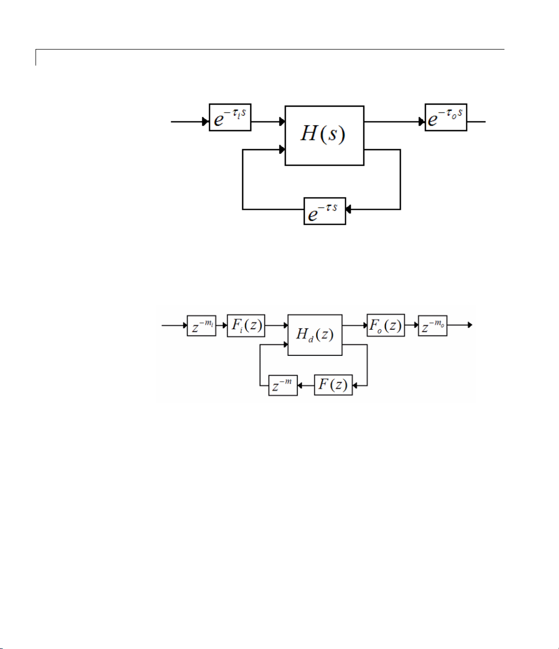
For example, the following figure illustrates a general SISO state-space
model H(s). H(s)hasinputdelayτ

,outputdelayτo, and internal delay τ.

i

2-45

c2d

The following figure shows the general result of discretizing the
state-space model using the
the general result is similar, except that the

tustin method. (For the matched method,

matched method does not

support internal delays.)

2-46

If Frac
the ti
are co
of the
m =ro

If
port

Fra

app

tDelayApproxOrder = 0

me delays to pure integer time delays. The resulting delays

mputed by rounding the time delay to the nearest multiple

sample time T
und(τ/T

actDelayApproxOrder > 0

Fr

).. In this case, Fi(z)=Fo(z)=F(z)=1.

s

: mi= round(τi/Ts), mo= round(τo/Ts), and

s

ion of the time delays by Thira n filters F

ctDelayApproxOrder

determines how much of the total delay c2d

roximatedbythefractionaldelayfilter, and how much is realized by

(its default value), c2d converts

,thenc2d approximates the fractional

(z), Fo(z), and F(z).

i

a chain of unit delays. For example, for the input delay τi,theorderof
the Thiran filter F

(z)is:

i

c2d

order(F

If ceil(τ

F

(z) approximates the entire input delay τi.Ifceil(τi/Ts)>

i

FractDelayApproxOrder, the Thiran filter only approximates a portion

of the input delay. In that case,
input delay as a chain of unit delays z

m

c2d uses T hiran filters and FractDelayApproxOrder in a similar way to

approximate the output delay τ

When discretizing

(z)) = max(ceil(τi/Ts), Fra ctDe layApproxOrder).

i

)<FractDelayApproxOrder,theThiranfilter

i/Ts

c2d represents the remainder of the

–m

,where

i

=ceil(τi/Ts)–FractDelayApproxOrder.

i

and the internal delay τ.

o

tf and zpk models using the tus tin or matched

methods, c2d first aggregates all input, output, and i/o delays into a
single i/o delay τ

for each channel. c2d then approximates τ

TOT

TOT

as a
Thiran filter and a chain of unit delays in the same way as described for
each of the time delays in

For more information about Thiran filters, see the

ss models.

thiran reference

page.

For more information about the Tustin and zero-pole matching
discretization methods, see “Converting Between Continuous- and
Discrete-Time Representations” in the Control System Toolbox User’s
Guide.

References [1] Franklin, G.F., Powell, D.J., and Workman, M.L., Digital Control of

Dynamic Systems (3rd Edition), Prentice Hall, 1997.

[2] L.F. Shampine and P. Gahinet, "Software for Modeling and Analysis
of Linear Systems with Delays," Proceedings of the American Control
Conference, 2004.

See Also c2dOptions, d2c, d2d, thiran

2-47

c2dOptions

Purpose Create option set for continuous- to discrete-time conversions

Syntax opts = c2dOptions

opts = c2dOptions('OptionName', OptionValue)

Description opts = c2dOptions returns the default options for c2d.

opts = c2dOptions('OptionName', OptionValue) accepts one or

more comma-separated name/value pairs that specify options for the

c2d command. Specify OptionName inside single quotes.

Input
Arguments

Name/Value Pairs

Method

Discretization method, specified as one of the following values:

'zoh'

'foh'

'impulse'

Zero-order hold, where c2d assumes the control
inputs are piecewise constant over the sampling
period

Triangle approximation (modified first-order
hold), where
piecewise linear over the sampling period
(See [1], p. 228.)

Impulse-invariant discretization.

Ts.

c2d assumes the control inputs are

Ts.

2-48

c2dOptions

'tustin'

Bilinear (Tustin) approximation. By default,

c2d discretizes with no prewarp and rounds

any fractional time delays to the nearest
multiple of the samp le time. To include
prewarp, use the

PrewarpFrequency option.

To approximate fractional tim e delays, use
the

FractDelayApproxOrder option.

'matched'

Zero-pole matching method. (See [1], p. 224.)
By default,

c2d rounds any fractional time

delays to the nearest multiple of the sample
time. To approximate fractional time delays, use
the

FractDelayApproxOrder option.

Default:

PrewarpFrequency

'zoh'

Prewarp frequency for 'tustin' method, specified in radians per
second. Takes positive scalar values. A value of 0 corresponds to
the s tandard

'tustin' method without prewarp.

Default: 0

FractDelayApproxOrder

Maximum order of the Thiran filter used to approximate fractional
delays in the
values. A value of 0 means that

'tustin' and 'matched' methods. Takes integer

c2d rounds fractional delays to

the nearest integer multiple of the sample time.

Default: 0

For additional information about the options and how to use them, see
“Converting Between Continuous- and Discrete-Time Representations”
in the Control System Toolbox User’s Guide and the

c2d reference page.

2-49

c2dOptions

Examples Discretize two models using identical discretization options.

% generate two arbitrary continuous-t ime state-space models
sys1 = rss(3, 2, 2);
sys2 = rss(4, 4, 1);

Use c2dOp tion s to create a set of discretization options.

opt = c2dOptions('Method', 'tustin', 'PrewarpFrequency', 3.4);

Then, discretize both models using the option set.

dsys1 = c2d(sys1, 0.1, op t); % 0.1s sampling time
dsys2 = c2d(sys2, 0.2, opt ); % 0.2s sampling time

The c2dOptions option set does not include the sampling time Ts.You
can use the same discretization options to discretize systems using a
different sampling time.

References [1] Franklin, G.F., Powell, D.J., and Workman, M.L., Digital Control of

Dynamic Systems (3rd Edition), Prentice Hall, 1997.

See Also c2d

2-50

Purpose State-space canonical realization

Syntax csys = canon(sys,'modal')

csys = canon(sys,'modal',CONDT)
csys = canon(sys,'companion')
[csys,T] = canon(sys,'type’)

Description canon computes a canonical state-space m odel for the continuo us or

discrete LTI system

Modal Form

csys = canon(sys,'modal') returns a realization csys in modal form.

If A has no repeated eigenvalues, the real eigenvalues appear on the
diagonal of the A matrix and the complex conjugate eigenvalues appear
in 2-by-2 block s on the diagonal of A. For a system with eigenvalues

(, , )

 

± j

12



000

⎡

1

⎢



00

⎢
⎢



00

−

⎢

000

⎣

sys. Two types of canonical forms are supported.

,themodalA matrix is of the form

⎤
⎥
⎥
⎥
⎥



2

⎦

canon

csys = canon(sys,'modal',CONDT) specifies an upper bound CONDT

on the condition number of the block-diagonalizing transformation T.
The default value is
eigenvalue clusters (setting

CONDT=1e8. Increase CONDT to reduce the size of the

CONDT=Inf amounts to diagonalizing A).

Companion Form

csys = canon(sys,'companion') produces a companion realization

of

sys where the characteristic polynomial of the system appears

explicitly in the rightmost column of the A matrix. For a system with
characteristic polynomial

ps s s s

nn

()=+ ++ +

−

1



1

…

nn

−

1

2-51

canon

the corresponding companion A matrix is

00 0

⎡
⎢
⎢
⎢

A

=

⎢⎢
⎢
⎢
⎢
⎣

.. ..

100 0 1
010

:::

010
001

0

..

..

.. ..

..

.

−



⎤

n

−−

::

⎥



n

⎥
⎥
⎥
⎥
⎥

−



2

⎥

−



1

⎦

For state-space models sys,

[csys,T] = canon(sys,'type’)

also returns the state coordinate transformation T relating the original
state vector x and the canonical state vector x

xTx

=

c

,where

c

This syntax is meaningful only when sys is a state-space model.

Algorithm Transfer functions or zero-pole-gain models are first conv erted to state

space using

The transformation to modal form uses the matrix P of eigenvectors of
the A matrix. The modal form is then obtained as

ss.

2-52

−−11



xPAPxPBu

=+

cc

yCPx Du

=+

c

The state transformation T returned is the inverse of P.

The reduction to companion form uses a state similarity transformation
based on the controllability matrix [1].

canon

Limitations The companion transformation requir es that the system be controllable

from the first input. The companion form is often p oo rly conditioned for
most state-space computations; avoid using it when possible.

References [1] Kailath, T. Linear Systems, Prentice-Hall, 1980.

See Also ctrb, ctrbf, ss2ss

2-53

care

Purpose Solve continuous-time algebraic Ricca ti equation

Syntax [X,L,G] = care(A,B,Q)

[X,L,G] = care(A,B,Q,R,S,E)
[X,L,G,report] = care(A,B,Q,...)
[X1,X2,D,L] = care(A,B,Q,...,'factor')

Description [X,L,G] = care(A,B,Q) computes the unique solution X of the

continuous-time algebraic Riccati equation

TT

A X XA XBB X Q

+− +=0

GRBXE

The care function also returns the gain matrix,

[X,L,G] = care(A,B,Q,R,S,E) solves the more general Riccati

equation

=

−1

T

.

TT T TT

A XE E XA E XB S R B XE S Q

+− + ++=

()( )10

−

When omitted, R, S,andE are set to the default va lues R=I, S=0,
and

E=I. Along with the solution X, care returns the gain matrix

TT

−1

GR BXES

=+

()

L=eig(A-B*G,E)

[X,L,G,report] = care(A,B,Q,...)

• -

1 when the associated Hamiltonian pencil has eigenvalues on or

and a vector L of closed-loop eigenvalues, where

returns a diagnosis report with:

very near the imaginary axis (failure)

• -

2 whenthereisnofinitestabilizingsolutionX

• The Frobenius norm of the relative residual if X exists and is finite.

This syntax does not issue any error message when X fails to exist.

[X1,X2,D,L] = care(A,B,Q,...,'factor') returns two matrices X1,
X2 and a diagonal scaling matrix D such that X = D*(X2/X1)*D.

2-54

The vector L contains the closed-loop eigenvalues. All outputs are
empty when the associated Hamiltonian matrix has eigenvalues on
the imaginary axis.

Examples Example 1

Given

−

32

⎡

ABCR=

⎢

11

⎣

you can solve the Riccati equation

TTT

A X XA XBR B X C C

+− + =−10

by

a = [-3 2;1 1]
b=[0;1]
c = [1 -1]
r=3
[x,l,g] = care(a,b,c'*c,r)

care

0

⎡

⎤
⎥

⎦

⎤

=

⎢

⎥

1

⎣

⎦

=−

11 3

[]

=

This yields the solution

x

x=

0.5895 1.8216

1.8216 8.8188

You can verify that this solution is indeed stabilizing by comparing
the eigenvalues of

[eig(a) eig(a-b*g)]

ans =

-3.4495 -3.5026

a and a-b*g.

2-55

care

1.4495 -1.4370

Finally, note that the variable l contains the closed-loop eigenvalues

eig(a-b*g).

l

l=

-3.5026

-1.4370

Example 2

-like Riccati equation

To solve the

H

∞

TTTT

AX XA X BB BB X CC

++ − + =

−

2

()γ

11 22

0

rewrite it in the care format as

1

−

T

AX XA XBB

+−

[, ]

12



B

2

⎡

I

−

γ

⎢

0

⎢

⎣



R

0

I

T

⎡

B

1

⎢

T

⎢

B

⎣

2

⎤
⎥
⎥

⎦

T

XXCC

+=0

⎤
⎥

⎥

⎦

You can now compute the stabilizing solutionXby

B = [B1 , B2]
m1 = size(B1,2)
m2 = size(B2,2)
R = [-g^2*eye(m1) zeros(m1,m2) ; zero s(m2 ,m1) eye(m2)]

X = care(A,B,C'*C,R)

Algorithm care implements the algorithms described in [1]. It works with the

EI=

Hamiltonian matrix when R is well-conditioned and
uses the extended Hamiltonian pencil and QZ algorithm.

;otherwiseit

2-56

care

Limitations The

(,)AB

controllable). In addition, the associated Hamiltonian matrix or pencil
must have no eigenvalue on the imaginary axis. Sufficient conditions

for this to hold are

⎡
⎢

SR

⎢

⎣

pair must be stabilizable (that is, all unstable modes are

QS

⎤
⎥

T

⎥

⎦

> 0

(, )QA

detectable when

S = 0

and

R > 0

,or

References [1] Arnold, W.F., III and A.J. Laub, "Generalized Eigenproblem

Algorithms and Software for Algebraic Riccati Equations," Proc. IEEE,
72 (1984), pp. 1746-1754

See Also dare, lyap

2-57

chgunits

Purpose Change frequency units of FRD model

Syntax sys = chgunits(sys,units)

Description sys = chgunits(sys,units) converts the units of the frequency

points stored in an FRD model,
of the strings
frequencies by applying the appropriate (

'Units' property is updated.

'Units' field already matches units, no conversion is made.

If the

'Hz' or 'rad/s'. This operation changes the ass igned

Example w = logspace(1,2,2);

sys = rss(3,1,1);
sys = frd(sys,w)
From input 'input 1' to:

Frequency(rad/s) output 1

---------------- -------­10 0.293773+0.00 1033i

100 0.294404+0.000 109i
Continuous-time frequency response data.
sys = chgunits(sys,'Hz')
sys.freq
ans =

1.5915

15.9155

sys to units,whereunits is either

2*pi) scaling factor, and the

See Also frd, get, set

2-58

Purpose Form model with complex conjugate coefficients

Syntax sysc = conj(sys)

Description sysc = conj(sys) constructs a complex conjugate model sysc by

applying complex conjugation to all coefficients of the LTI model

sys. This function accepts LTI models in transfer function (TF),

zero/pole/gain (ZPK), and s tate space (SS) formats.

Example If sys is the transfer function

(2+i)/(s+i)

then conj(sys) produces the transfer function

(2-i)/(s-i)

This operation is useful for manipulating partial fraction expansions.

conj

See Also append, ss, tf, zpk

2-59

connect

Purpose Arbitrary interconnection of LTI models

Syntax sys = connect(sys1,sys2,...,inputs,outputs)

sys = connect(blksys,Q,inputs,outputs)

Description connect constructs the aggregate model for a given block diagram

interconnection of LTI models. You can specify the block diagram
connectivity in two ways:

• Name-based interconnection

• Index-based interconnection

Name-Based Interconnection

In this approach, you name the input and output signals of all LTI
blocks
blocks. The aggregate model

sys1, sys2,... in the block diagram, including the summation

sys is then built by

2-60

sys = connect(sys1,sys2,...,inputs,outputs)

where inputs and outputs are the names of the block diagram external
I/Os, specified as strings or cell arrays of strings.

Note For MIMO systems, you can use strseq to quickly generate
numbered channel names as a sequence of indexed strings, for example

{'e1','e2','e3'}.

Example of Name-Based Interconnection

Given LTI models C and G in the following block diagram,

connect

construct the closed-loop model T from r to y.

C.InputName = 'e'; C .Out putName = 'u';
G.InputName = 'u'; G. Outp utName = 'y';
Sum = sumblk('e','r','y','+-');
T = connect(G,C,Sum,'r','y')

Index-Based Interconnection

In this approach, first combine all LTI blocks into an aggregate,
unconnected model
where each row specifies one of the connections or summing junctions in
terms of the input vector
the row

blksys using append. Then, construct a matrix Q

u and output vector y of blksys. For example,

[3 2 0 0]

indicates that y(2) feeds into u(3), while the row

[7 2 -15 6]

indicates that y(2)-y(15)+y(6) feeds into u(7). The aggregate model

sys is then obtained by

sys = connect(blksys,Q,inputs,outputs)

where inputs and outputs are index vectors into u and y selecting
the block diagram external I/Os.

2-61

connect

Example of Index-Based Interconnection

Construct the closed-loop model T for the previous block diagram.

blksys = append(C,G);
% u = inputs to C,G. y = outputs of C,G.
% Here y(1) feeds into u(2) and -y(2) feeds into u(1)
Q = [2 1; 1 -2];
% External I/Os: r drives u(1) and y is y(2)
T = connect(blksys,Q,1,2)

Verify that you entered all of the model information correctly by
checking the following items:

• Poles of the unconnected model

blocks in the diagram.

• Final poles and DC gains are reasonable.

• Plots of the

step and bode responses of sysc are as expected.

sys match the poles of the various

Delays

The connect function supports I/O and internal delays. See Time
Delays for more information and examples.

Example Construct the model shown in thefollowingblockdiagram.

2-62

connect

.

Use the matrices of the following state-space model

A = [ -9.0201 17.7791

-1.6943 3.2138 ];

B = [ -.5112 .5362

-.002 -1.8470];

C = [ -3.2897 2.4544

-13.5009 18.0745];

D = [-.5476 -.1410

-.6459 .2958 ];

1 Define the three blocks in the block diagram as individual LTI models

sys2:

by typing the following commands:

sys1 = tf(10,[1 5],'inputname','uc')
sys2 = ss(A,B,C,D,'inputname',{'u1' 'u2'},...

'outputname',{'y1' 'y2'})

sys3 = zpk(-1,-2,2)

2 Append the blocks to form the unconnected model sys by typing the

following command:

sys = append(sys1,sys2,sys3)

This command returns the following block-diagonal model:

sys

a=

x1 x2 x3 x4
x1 -5 0 0 0
x2 0 -9.0 2 17.78 0
x3 0 -1.694 3.214 0
x4 0 0 0 -2

b=

2-63

connect

uc u1 u2 ?
x14000
x2 0 -0.5112 0.5362 0
x3 0 -0.002 -1.847 0
x40002

c=

x1 x2 x3 x4
?2.5000
y1 0 -3.29 2.454 0
y2 0 -13.5 18.07 0
? 000-1

d=

uc u1 u2 ?
? 0000
y1 0 -0.5476 -0.141 0
y2 0 -0.6459 0.2958 0
? 0002

2-64

Continuous-time model.

Note that the ordering of the inputs and outputs matches the block
ordering you chose. A question mark (

?) denotes an unnamed input

or output.

3 Specify the matrix Q for connections of outputs 1 and 4 into input 3

(

u2), a nd output 3 (y2) into input 4 by typing the following syntax:

Q=[31-4

4 3 0];

Note that the second row of Q is padded with a trailing zero.

4 Specify the two external inputs, uc and u1 (inputs 1 and 2 of sys),

and the two external outputs,

y1 and y2 (outputs 2 and 3 of sys),

by typing the following syntax:

connect

inputs = [1 2];
outputs = [2 3];

5 Create a state-space model for the overall interconnection by typing

the following syntax:

sysc = connect(sys,Q,inputs,outputs)

a=

x1 x2 x3 x4
x1-5000
x2 0.8422 0.07664 5.601 0.3369
x3 -2.901 -33.03 45.16 -1.16
x4 0.9293 -16.97 22.71 -1.628

b=

uc u1
x1 4 0
x2 0 -0.076
x3 0 -1.501
x4 0 -0.8116

c=

x1 x2 x3 x4
y1 -0.2215 -5.682 5.657 -0.08859
y2 0.46 46 -8.483 11.36 0.1859

d=

uc u1
y1 0 -0.662
y2 0 -0.4058

Continuous-time model.

2-65

connect

Note Blocks and states that are not connected to inputs or outputs are

automatically discarded.

References [1] Edwards, J.W., "A Fortran Program for the Analysis of Linear

Continuous and Sampled-Data Systems," NASA Report TM X56038,
Dryden Research C enter, 1976.

See Also sumblk, strseq, append, feedback, minreal, parallel, ser ies, lft

2-66

Purpose Output and state covariance of system driven by white noise

Syntax P = covar(sys,W)

[P,Q] = covar(sys,W)

Description covar calculates the stationary covariance of the output y of an LTI

model
handles both continuous- and dis crete-time cases.

P = covar(sys,W) returns the steady-state output response covariance

sys driven by Gaussian white noise inputs w. This function

covar

PEyy

= ()

given the noise intensity

Ewtw W t

(()()) ( )

Ewkwl W

[P,Q] = covar(sys,W) als o returns the steady-state state covariance

QExx

= ()

when sys is a state-space model (otherwise Q is set to []).

When applied to an
multidimensional arrays P, Q such that

P(:,:,i1,...iN) and Q(:,:,i1,...iN) are the covariance matrices

for the model

T

T



=−

()

[] []

T



=

kl

T

N-dimensional LTI array sys, covar returns

sys(:,:,i1,...iN).

(continuous time)

(disccrete time)

Example Compute the output response covariance of the discrete SISO system

21

z

Hz

()

+

2

02 05

zz

++

..

,.=

01

T

=

s

duetoGaussianwhitenoiseofintensityW=5.Type

2-67

covar

sys = tf([2 1],[1 0.2 0.5],0.1);
p = covar(sys,5)

These commands produce the following result.

p=

30.3167

You can compare this output of covar to simulation results.

randn('seed',0)
w = sqrt(5)*randn(1,1000); % 1000 samples

% Simulate response to w with LSIM:
y = lsim(sys,w);

% Compute covariance of y values
psim = sum(y .* y)/length(w);

This yields

psim =

32.6269

The tw o covariance values p and psim do not agree perfectly due to the
finite simulation horizon.

Algorithm Transfer functions and zero-pole-gain models are first converted to

2-68

state space with

For continuous-time state-space models



xAxBw

=+

yCxDw

=+

Q is obtained by solving the Lyapunov equation

ss.

covar

AQ QA BWB

The output response covariance P is finite only when D = 0 and then
P = CQC

In discrete time, the state covariance solves the discrete Lyapunov
equation

AQA Q BWB

and P is given by P = CQCT+ DWD

Note that P is well defined for nonzero D in the discrete case.

TT

++ =0

T

.

TT

−+ =0

T

Limitations The state and output covariances are defined for stable systems only.

For continuous systems, the output response covariance P is finite only
when the D matrix is zero (strictly proper system).

References [1] Bryson, A.E. and Y.C. Ho, Applied O ptimal Control, Hemisphere

Publishing, 1975, pp. 458-459.

See Also dlyap, lyap

2-69

ctrb

Purpose Controllability matrix

Syntax Co = ctrb(sys)

Description ctrb computes the controllability matrix for state-space systems. For

an n-by-n matrix
controllability matrix

⎡

Co BABAB A B

=

⎣

where Co has n rows and nm columns.

Co = ctrb(sys) calcu l ates the controllability matrix of the state-space

LTI object

Co = ctrb(sys.A,sys.B)

The system is controllable if Co has full rank n.

sys. Thissyntaxisequivalenttoexecuting

A and an n-by-m matrix B, ctrb( A,B) returns the

n

−21

…

⎤
⎦

(2-1)

Example Check if the system with the following data

A=

11
4-2

B=

1-1
1-1

is controllable. Type

Co=ctrb(A,B);

% Number of uncontrollable states
unco=length(A)-rank(Co)

These commands produce the following result.

2-70

unco =

1

Limitations Estimating the rank of the controllability matrix is ill-conditioned; that

is, it is very sensitive to roundoff errors and errors in the data. An
indication of this can be seen from this simple example.



1

⎡
⎢

01

⎣

⎤

,

⎥
⎦

⎡

=

⎢
⎣

AB=

This pair is controllable if
relative machine precision.

BAB

[]

which is not full rank. For cases like these, it is better to determine the
controllability of a system using

=

11



1

⎡

⎤

⎢

⎥



⎣

⎦





≠ 0

but if

ctrb(A,B) returns

⎤
⎥

⎦

ctrbf.

< eps

,whereeps is the

ctrb

See Also ctrbf, obsv

2-71

ctrbf

Purpose Compute controllability staircase form

Syntax [Abar,Bbar,Cbar,T,k] = ctrbf(A,B,C)

ctrbf(A,B,C,tol)

Description If the controllability matrix of (A , B)hasrankr ≤ n,wheren is the size

of A, then there exists a similarity transformation such that

ATAT BTBCCT

TT

===,,

where T is unitary, and the transformed system has a staircase form,
in which the uncontrollable modes, if there are any, are in the upper
left corner.

A

⎡

A

=

⎢
⎣

00

uc

AA

21

⎤

,,

⎥

cc

⎦

⎡

⎤

=

B

⎢

B

⎣

=

CCC

⎥
⎦

[]

nc c

where (Ac, Bc) is controllable, all eigenvalues of Aucare uncontrollable,

CsI A B CsI A B

and

[Abar,Bbar,Cbar,T,k] = ctrbf(A,B,C) decomposes the state-space

() ()−=−

ccc

system represented by
form,

Abar, Bbar,andCbar, described above. T is the similarity

transformation matrix and
of the system represented by

−−11

A, B,andC into the controllability staircase

k is a vector of length n,wheren is the order

.

A.Eachentryofk repres ents the number

of controllable states factored out during each step of the transformation
matrix calculation. The number of nonzero elements in
how many iterations were necessary to calculate
number of states in A

ctrbf(A,B,C,tol) uses the tolerance tol when calculating the

, the controllable portion of Abar.

c

T,andsum(k) is the

k indicates

controllable/uncontrollable subspaces. When the tolerance is not
specified, it defaults to

10*n*norm(A,1)*eps.

Example Compute the controllability staircase form for

A=

2-72

11
4-2

B=

1-1
1-1

C=

10
01

and locate the uncontrollable mode.

[Abar,Bbar,Cbar,T,k]=ctrbf(A,B,C)

Abar =

-3.0000 0

-3.0000 2.0000

Bbar =

0.0000 0.0000

1.4142 -1.4142

ctrbf

Cbar =

-0.7071 0.7071

0.7071 0.7071

T=

-0.7071 0.7071

0.7071 0.7071

k=

10

The decomposed system Abar shows an uncontrollable mode located at

-3 and a controllable mode located at 2.

Algorithm ctrbf implements the Staircase Algorithm of [1].

2-73

ctrbf

References [1] Ros enbrock, M.M., State-Space and Multivariable Theory,John

Wiley, 1970.

See Also ctrb, minreal

2-74

ctrlpref

Purpose Set Control System Toolbox preferences

Syntax ctrlpref

Description ctrlpref opens a Graphical User Interface (GUI) which allows you to

change the Control System Toolbox preferences. Preferences set in this
GUI affect future plots only (existing plots are not altered).

Your preferences are stored to disk (in a system-dependent location)
and will be automatically reloaded in future MATLAB
the Control System Toolbox software.

See Also sisotool, ltiview

®

sessions using

2-75

d2c

Purpose Convert from discrete- to continuous-time models

Syntax sysc = d2c(sysd)

sysc = d2c(sysd,'method')
sysc = d2c(sysd, opts)

Description sysc = d2c(sysd) produces a continuous-time model sysc that is

equivalent to the discrete-time LTI model
the inputs.

sysc = d2c(sysd,'method') uses the specified conversion method
'method':

sysd using zero-order hold on

'zoh'

'tustin'

'matched'

sysc = d2c(sysd, opts) converts sysd using the option set specified

with

d2cOptions object.

See “Converting Between Continuous- and Discrete-Time
Representations” for more details on the conversion methods.

Usage • Use the

the de

uency prewarp (formerly the

afreq

x

synta

and “Converting Between Continuous- and Discrete-Time

page

esentations” in the C ontrol System Toolbox User’s Guide.

Repr

Zero-order hold on the inputs. The control inputs are
assumed piecewise constant over the sampling period.

Bilinear (Tustin) approximation to the derivative.

Zero-pole matching method of [1] (for SISO systems only).

syntax

fault options for

sysc = d2c(sysd, opts).Seethed2cOptions reference

sysc = d2c(sysd, 'method') to convert sysd using

'method'.Tospecifytustin conversion with

'prewarp' method), use the

2-76

Example Consider the discrete-time model with transfer function

z

Hz

=

()

and sample time Ts= 0.1 s. You can derive a continuous-time
zero-order-hold equivalent model by typing

Hc = d2c(H)

Discretizing the resulting model Hc with the default zero-order hold
method and sampling time T
H(z):

c2d(Hc,0.1)

To use the Tustin approximation i ns te ad of zero-order hold, type

Hc = d2c(H,'tustin')

−

zz

++1032.

= 0.1s returns the original discrete model

s

d2c

As with zero-order hold, the inverse discretization operation

c2d(Hc,0.1,'tustin')

gives back the original H(z).

Algorithm d2c performs the 'zoh' conversion in state space, and relies on the

matrix logarithm (see

logm in the MATLAB documentation).

Limitations The Tustin approximation is not defined for systems with poles at z =–1

and is ill-conditioned for systems with poles near z =–1.

The zero-order hold method cannot handle systems with poles at z =0.
In addition, the
with negative real poles , [2]. The model order increases because the
matrix logarithm maps real negative poles to complex p ole s. Single
complex poles are not physically meaningful because of their complex
time response.

'zoh' conversion increases the model order for systems

2-77

d2c

Instead, to ensure that all complex poles of the continuous model
come in conjugate pairs,

d2c replaces negative real poles z =–α with

a pair of complex conjugate poles near –α. The conversion then yields
a continuous model with higher order. For example, to convert the
discrete-time transfer function

02

.

z

Hz

()

=

zzz

()

+

2

05 04

+

++

..

()

type:

Ts = 0.1 % sample time 0.1 s
H = zpk(-0.2,-0.5,1,Ts) * tf(1,[1 1 0.4],Ts)
Hc = d2c(H)

These commands produce the following result.

Warning: System order was increased to handle real negative poles.

2-78

Zero/pole/gain:

-33.6556 (s-6.273) (s^2 + 28.29s + 1041)

--------------------------------------------

(s^2 + 9.163s + 637.3) (s^2 + 13.86s + 1035)

To convert Hc back to discrete time, type:

c2d(Hc,Ts)

yielding

Zero/pole/gain:

(z+0.5) (z+0.2)

------------------------­(z+0.5)^2 (z^2 + z + 0.4)

Sampling time: 0.1