Mathworks COMMUNICATIONS TOOLBOX 4 user guide

Download

Communications To

User’s Guide

olbox™ 4

How to Contact The MathWorks

www.mathworks. comp.soft-sys.matlab Newsgroup www.mathworks.com/contact_TS.html Technical Support

suggest@mathworks.com Product enhancement suggestions bugs@mathwo doc@mathworks.com Documentation error reports service@mathworks.com Order status, license renewals, passcodes info@mathwo

com

rks.com

Web

Bug reports

Sales, prici

ng, and general information

508-647-7000 (Phone)

508-647-7001 (Fax)

The MathWorks, Inc. 3 Apple Hill Drive Natick, MA 01760-2098

For contact information about worldwide offices, see the MathWorks Web site.

Communications Toolbox™ User’s Guide

The software described in this document is furnished under a license agreement. The software may be used or copied only under the terms of the license agreement. No part of this manual may be photocopied or reproduced in any form without prior written consent from The MathW orks, Inc.

FEDERAL ACQUISITION: This provision applies to all acquisitions of the Program and Documentation by, for, or through the federal government of the United States. By accepting delivery of the Program or Documentation, the government hereby agrees that this software or documentation qualifies as commercial computer software or commercial computer software documentation as such terms are used or defined in FAR 12.212, DFARS Part 227.72, and DFARS 252.227-7014. Accordingly, the terms and conditions of this Agreement and only those rights specified in this Agreement, shall pertain to and govern theuse,modification,reproduction,release,performance,display,anddisclosureoftheProgramand Documentation by the federal government (or other entity acquiring for or through the federal government) and shall supersede any conflicting contractual terms or conditions. If this License fails to meet the government’s needs or is inconsistent in any respect with federal procurement law, the government agrees to return the Program and Docu mentation, unused, to The MathWorks, Inc.

Trademarks

MATLAB and Simulink are registered trademarks of The MathWorks, Inc. See

www.mathworks.com/trademarks for a list of additional trademarks. Other product or brand

names may be trademarks or registered trademarks of their respective holders.

Patents

The MathWorks products are protected by one or more U.S. patents. Please see

www.mathworks.com/patents for more information.

Revision History

April 1996 First printing Version 1.0 May 1997 Second printing Revised for Version 1.1 (MATLAB 5.0) September 2000 Third printing Revised for Version 2.0 (Release 12) May 2001 Online only Revised for Version 2.0.1 (Release 12.1) July 2002 Fourth printing Revised for Version 2.1 (Release 13) June 2004 Fifth printing Revised for Version 3.0 (Release 14) October 2004 Online only Revised for Version 3.0.1 (Release 14SP1) March 2005 Online only Revised for Version 3.1 (Release 14SP2) September 2005 Online only Revised for Version 3.2 (Release 14SP3) October 2005 Reprint Version 3.0 (Notice updated) March 2006 Online only Revised for Version 3.3 (Release 2006a) September 2006 Sixth printing Revised for Version 3.4 (Release 2006b) March 2007 Online only Revised for Version 3.5 (Release 2007a) September 2007 Online only Revised for Version 4.0 (Release 2007b) March 2008 Online only Revised for Version 4.1 (Release 2008a) October 2008 Online only Revised for Version 4.2 (Release 2008b) March 2009 Online only Revised for Version 4.3 (Release 2009a) September 2009 Online only Revised for Version 4.4 (Release 2009b) March 2010 Online only Revised for Version 4.5 (Release 2010a)

Getting Started

Product Overview ................................. 1-2

Section Overview Expected Background

.................................. 1-2

.............................. 1-2

Contents

Studying Components of a Communication System

Section Overview Modulating a Random Signal Plotting Signal Constellations Pulse Shaping Using a Raised Cosine Filter Using a Convolutional Code

Simulating a Communication System

Section Overview Using BERTool to Run Simulations Varying Parameters and Managing a Se t of Simulations

Running Simulations Using the Error Rate Test

Console

Loading the Error Rate Test Console Running the Simulation and Obtaining Results Generating an Error Rate Results Figure Window Running the Simulation Using Parallel Computing Toolbox

Software

Creating a System File and Attaching It to the Test

Console

Configuring the Error Rate Test Console and Running a

Simulation

Optimizing Your System for Faster Simulations

......................................... 1-35

.................................. 1-4

........................ 1-4

....................... 1-11

............ 1-15

......................... 1-19

................ 1-23

.................................. 1-23

................... 1-23

.................. 1-35

......... 1-36

....... 1-37

....................................... 1-39

....................................... 1-40

..................................... 1-45

........ 1-47

... 1-4

.. 1-31

Learning M ore

Online Help Demos The MathWorks Online

.......................................... 1-54

.................................... 1-54

...................................... 1-54

............................ 1-54

Signal Sources

White G aussian Noise .............................. 2-2

Random Symbols

Random Integers

Random Bit Error Patterns

.................................. 2-3

.................................. 2-4

......................... 2-5

Performance Evaluation

Performance Results via Simulation ................ 3-2

Section Overview Using Simulated Data to Compute Bit and Sym bol Error

Rates Example: Computing Error Rates Comparing Symbol Error Rate and Bit Error Rate

Performance Results via the Semianalytic

Technique

Section Overview When to Use the Semianalytic Technique Procedure for the Semianalytic Technique Example: Using the Semianalytic Technique

......................................... 3-2

.................................. 3-2

.................... 3-3

....... 3-4

...................................... 3-5

.................................. 3-5

.............. 3-5

............. 3-6

........... 3-7

vi Contents

Theoretical Performance Results

Computing Theoretical Error Statistics Plotting Theoretical Error Rates Comparing Theoretical and Empirical Error Rates

Error Rate Plots

Section Overview Creating Error Rate Plots Using Curve F itting for Error Rate Plots

................................... 3-14

.................................. 3-14

................... 3-10

................ 3-10

..................... 3-10

semilogy ............. 3-14

.................... 3-15

...... 3-11

Example: Curve Fitting for an Error Rate Plot ......... 3-15

Eye Diagrams

Section Overview EyeScope

Scatter P lots

Section Overview Viewing Signals Using Scatter Plots

Adjacent Channel Power Ratio (ACPR)

Measurements

Overview o f ACPR Measurement Tutorial

EVM Measurements

Section Overview

MER Measurements

Section Overview

Selected Bibliography for Performance Evaluation

..................................... 3-20

.................................. 3-20

........................................ 3-20

...................................... 3-21

.................................. 3-21

.................. 3-21

.................................. 3-34

............. 3-34

................................ 3-44

.................................. 3-44

................................ 3-45

.................................. 3-45

... 3-46

Error Rate T est Console

Introduction to Error Rate Test Console ............. 4-2

Creating a System

Writing A Register Method Writing a Setup Method Writing a Reset Method Writing a Run Method

Methods Allowing You to Communicate with the Error

Rate Test Console at Simulation Run Time

Getting Test Inputs From the Error Rate Test Console

................................. 4-3

.......................... 4-3

............................ 4-6

............................. 4-6

........ 4-8

... 4-8

vii

Getting the Current Simulation Sweep Value of a

Registered Test Parameter Logging Test Data to a Registered Test Probe Logging User-Defined Data To The Test Console

........................ 4-9

.......... 4-9

........ 4-9

Debug Mode

Implementing A Default Input Generator Function For

Debug Mode

Running Simulations Using the Error Rate Test

Console

Creating a Test Console Attaching a System to the Error Rate Test Console Defining Simulation Conditions Registering a Test Point Getting Test Information Running a Simulation Getting Results and Plotting Data Parsing and Plotting Results for Multiple Parameter

Simulations

....................................... 4-10

.................................... 4-10

......................................... 4-11

............................ 4-11

...... 4-12

...................... 4-13

............................ 4-15

........................... 4-16

.............................. 4-17

.................... 4-17

.................................... 4-17

BERTool: A Bit Error Rate Analysis GUI

Summary of Features .............................. 5-2

viii Contents

Opening BERTool

The BERTool Environment

Components of BERTool Interaction Among BERTool Components

Computing Theoretical BERs

Section Overview Example: Using the Theoretical Tab in BERTool Available Sets of Theoretical BER Data

................................. 5-3

......................... 5-4

............................ 5-4

....................... 5-8

.................................. 5-8

............... 5-11

.............. 5-6

........ 5-9

Using the Semianalytic Technique to Compute

BERs

Section Overview Example: Using the Semianalytic Tab in BERTool Procedure for Using the Semianalytic Tab in BERTool

........................................... 5-16

.................................. 5-16

...... 5-17

... 5-19

Running M AT LAB Simulations

Section Overview Example: Usin g a MATLAB Simulation with BERTool Varying the Stopping Criteria Plotting Confidence Intervals Fitting BER Points to a Curve

Preparing Simulation Functions for Use with

BERTool

Requirements for Functions Template for a Simulation Function Example: Preparing a Simulation Function for Use with

BERTool

Running Sim ulink Simulations

Section Overview Example: Using a Simulink Model with BERTool Varying the Stopping Criteria

Preparing Simulink Models for Use with BERTool

Requirements for Models Tips for Preparing Models Example: Preparing a Model for Use with BERTool

........................................ 5-29

.................................. 5-22

....................................... 5-33

.................................. 5-37

........................... 5-43

..................... 5-22

....................... 5-25

........................ 5-26

....................... 5-28

......................... 5-29

.................. 5-30

..................... 5-37

....... 5-38

....................... 5-41

.......................... 5-43

... 5-22

.... 5-43

..... 5-46

Managing BER Data

Exporting Data Sets or BERTool Sessions Importing Data Sets or BERTool Sessions Managing Data in the Data Viewer

............................... 5-52

............. 5-52

............. 5-55

................... 5-57

Source Coding

QuantizingaSignal ................................ 6-2

Section Overview Representing Partitions Representing Codebooks Scalar Quantization Example 1 Scalar Quantization Example 2 Determining Which Interval Each Input Is In

.................................. 6-2

............................ 6-2

............................ 6-3

...................... 6-3

...................... 6-4

.......... 6-4

Optimizing Quantization Parameters

Section Overview Example: Optimizing Quantization Parameters

Differential Pulse Code Modulation

Section Overview DPCM Terminology Representing Predictors Example: DPCM Encoding and Decoding

Optimizing DPCM Parameters

Section Overview Example: Comparing Optimized and Nonoptimized DPCM

Parameters

Companding a Signal

Section Overview Example: µ-Law Compander

Huffman Coding

Section Overview Creating a Huffman Code Dictionary Example: Creating and Decoding a Huffman Code

.................................. 6-6

.................................. 6-8

................................ 6-8

............................ 6-8

...................... 6-11

.................................. 6-11

.................................... 6-11

.............................. 6-13

.................................. 6-13

........................ 6-13

................................... 6-15

.................................. 6-15

................ 6-6

......... 6-6

................. 6-8

.............. 6-9

................. 6-15

...... 6-16

x Contents

Arithmetic Coding

Section Overview Representing Arithmetic Coding Parameters Example: Creating and Decoding an Arithmetic C ode

................................. 6-17

.................................. 6-17

........... 6-17

.... 6-18

Selected Bibliography for Source Coding ............ 6-19

Error Detection and Correction

Block Coding ...................................... 7-2

Section Overview Block Coding Features of the Toolbox Block Coding Terminology Representing Words for Reed-Solomon Codes Parameters for Reed-Solomon Codes Creating and Decoding Reed-Solomon Codes Representing Words for BCH Codes Parameters for BCH Codes Creating and Decoding BCH Codes LDPC Codes Representing Words for Linear Block Codes Parameters for Linear Block Codes Creating and Decoding Linear Block Codes Performing Other Block Code Tasks Selected Bibliography for Block Coding

.................................. 7-2

................. 7-4

.......................... 7-5

........... 7-5

.................. 7-6

........... 7-8

.................. 7-12

.......................... 7-13

................... 7-13

...................................... 7-15

............ 7-16

................... 7-20

............ 7-25

.................. 7-28

................ 7-31

Convolutional Coding

Section Overview Convolutional Coding Features of the Toolbox Polynomial Description of a Convolutional Encoder Trellis D escription of a Convolutional Encoder Creating and Decoding Convo lutio nal Codes Examples of Convolutional Coding Selected Bibliography for Convolutional Coding

Cyclic Redundancy Check Coding

Overview CRC Algorithm Selected Bibliography for CRC Coding

........................................ 7-46

.............................. 7-32

.................................. 7-32

................... 7-42

................... 7-46

................................... 7-46

................ 7-48

.......... 7-32

...... 7-32

.......... 7-36

........... 7-39

......... 7-45

Interleaving

Block Interleavers ................................. 8-2

Section Overview Block Interleaving Features of the Toolbox Example: Block Interleavers

.................................. 8-2

............. 8-2

........................ 8-3

Convolutional Interleavers

Section Overview Convolutional Interleaving Features of the Toolbox Example: Convolutional Interleavers Delays of Convolutional Interleavers

Selected Bibliography for Interleaving

.................................. 8-5

......................... 8-5

...... 8-6

................. 8-7

.................. 8-9

.............. 8-14

Modulation

Modulation Features of the Toolbox ................. 9-2

Modulation Techniques Baseband vs. Passband Simulation

Modulation Terminology

Analog Modulation

Representing Analog Signals Analog Modulation Example

............................. 9-2

................... 9-3

........................... 9-4

................................ 9-5

........................ 9-5

........................ 9-6

xii Contents

Digital Modulation

Section Overview Representing Digital Signals Baseband ModulatedSignalsDefined Gray Encoding a Modulated Signal Examples of Digital Modulation and Demodulation Plotting Signal Constellations

................................. 9-8

.................................. 9-8

........................ 9-8

................. 9-9

................... 9-10

....................... 9-14

...... 9-12

Using Modem Objects .............................. 9-20

Section Overview Constructing a Modem Object Managing Object Properties Copying a Modem Object Displaying a Modem O b ject Resetting a Modem Object Modulating a Signal Demodulating a Signal Example of Basic Modulation and Demodulation Exact LLR Algorithm Approximate LLR Algorithm

.................................. 9-20

....................... 9-20

......................... 9-21

........................... 9-21

......................... 9-22

.......................... 9-23

............................... 9-24

............................. 9-25

........ 9-26

.............................. 9-26

........................ 9-27

Selected Bibliography for Modulation

............... 9-28

Special Filters

Noncausality and the Group Delay Parameter ....... 10-2

Section Overview Example: Compensating for Group Delays in Data

Analysis

Designing Hilbert Transform Filters

Section Overview Example with Default Parameters

Filtering with Raised Cosine Filters

Section Overview Sampling Rates Designing Filters Automatically Specifying Filters Using Input A rguments Controlling the Rolloff Factor Controlling the Group Delay Combining Two Square-Root Raised Cosine Filters

.................................. 10-2

....................................... 10-3

................ 10-5

.................................. 10-5

................... 10-5

................. 10-7

.................................. 10-7

................................... 10-7

..................... 10-8

............. 10-9

........................ 10-10

...... 10-12

Designing Raised Cosine Filters

Section Overview Sampling Rates

.................................. 10-14

................................... 10-14

.................... 10-14

xiii

Example Designing a Square-Root Raised Cosine Filter .. 10-14 Other Options in Filter Design

....................... 10-15

Selected Bibliography for Special Filters

............ 10-16

Channels

Channel Features of the Toolbox .................... 11-2

AWGN Channel

Section Overview Describing the Noise Level of an AW GN Channel

MIMO Channels

Fading Channels

Section Overview Overview of Fading Channels Simulation of Multipath Fading Channels: Methodology Specifying Fading Channels Specifying the Doppler Spectrum of a Fading Channel Configuring Channel Objects Using Fading Channels Examples Using Fading Channels Using the Channel Visualization Tool

.................................... 11-3

.................................. 11-3

....... 11-3

................................... 11-6

.................................. 11-7

....................... 11-7

.. 11-9

......................... 11-11

... 11-15

........................ 11-20

............................ 11-23

.................... 11-24

................. 11-34

xiv Contents

Binary Symmetric Channel

Section Overview Example: Introducing Noise in a C onvolutional Code

Selected Bibliography for Channels

.................................. 11-48

......................... 11-48

................. 11-50

.... 11-48

Equalizer Features of Communications Toolbox

Software

........................................ 12-2

Equalizers

Overview of Adaptive Equalizer Classes

Section Overview Symbol-Spaced Equalizers Fractionally Spaced Equalizers Decision-Feedback Equalizers

Using Adaptive Equalizer Functions and Objects

Section Overview Basic Procedure for Equalizing a Signal Example Illustrating the Basic Procedure Learning More About Adaptive Equalizer Functions

Specifying an Adaptive Algorithm

Choosing an Adaptive Algorithm Indicating a Choice of Adaptive Algorithm Accessing Properties of an Adaptive Algorithm

Specifying an Adaptive Equalizer

Defining an Equalizer Object Accessing Properties of an Equalizer

Using Adaptive Equalizers

Section Overview Equalizing Using a Training Sequence Equalizing in Decision-Directed Mode Delays from Equalization Equalizing Using a Loop

.................................. 12-3

.......................... 12-3

...................... 12-5

....................... 12-6

.................................. 12-8

................... 12-10

..................... 12-10

................... 12-13

........................ 12-13

......................... 12-17

.................................. 12-17

........................... 12-21

............................ 12-22

............. 12-3

............... 12-8

.............. 12-8

............. 12-11

......... 12-12

.................. 12-14

................ 12-17

................. 12-19

..... 12-8

..... 12-9

Using MLSE Equalizers

Section Overview Equalizing a Vector Signal Equalizing in Continuous Operation Mode Using a Preamble or Postamble

.................................. 12-28

............................ 12-28

.......................... 12-29

...................... 12-33

............. 12-30

Selected Bibliography for Equalizers ................ 12-36

Galois Field Computations

Galois Field Terminology ........................... 13-3

Representing Elements of Galois Fields

Section Overview Creating a Galois Array Example: Creating Galois Field Variables Example: Representing Elements of GF(8) How Integers Correspond to Galois Field Elements Example: Representing aPrimitiveElement Primitive Polynomials and Element R epresentations

Arithmetic in Galois Fields

Section Overview Example: Addition and Subtraction Example: Multiplication Example: Division Example: Exponentiation Example: Elementwise Logarithm

Logical Operations in Galois Fields

Section Overview Testing for Equality Testing for Nonzero Values

Matrix Manipulation in Galois Fields

Basic Manipulations of Galois Arrays Basic Information About Galois Arrays

.................................. 13-4

............................ 13-4

......................... 13-14

.................................. 13-14

............................ 13-16

................................. 13-17

........................... 13-18

.................................. 13-20

............................... 13-20

......................... 13-21

.............. 13-4

............. 13-5

............. 13-7

.................. 13-15

................... 13-19

................. 13-20

................ 13-23

................. 13-23

................ 13-24

...... 13-8

........... 13-9

.... 13-9

xvi Contents

Linear Algebra in Galois Fields

Inverting Matrices and Computing Determinants Computing Ranks Factoring Square Matrices Solving Linear Equations

................................. 13-26

........................... 13-27

..................... 13-25

.......................... 13-26

....... 13-25

Signal Processing Operations in Galois Fields ........ 13-29

Section Overview Filtering Convolution Discrete Fourier Transform

......................................... 13-29

.................................. 13-29

...................................... 13-30

......................... 13-31

Polynomials over Galois Fields

Section Overview Addition and Subtraction of Polynomials Multiplication and Division of Polynomials Evaluating Polynomials Roots of Polynomials Roots of Binary Polynomials Minimal Polynomials

Manipulating Galois Variables

Section Overview Determining Whether a Variable Is a Galois Array Extracting Information from a Galois Array

Speed and Nondefault Primitive Polynomials

Selected Bibliography for Galois Fields

.................................. 13-33

............................ 13-34

............................... 13-35

.............................. 13-37

.................................. 13-39

..................... 13-33

.............. 13-33

............. 13-34

......................... 13-36

...................... 13-39

............ 13-39

.............. 13-44

EyeScope: An Eye Diagram Analysis Tool

...... 13-39

........ 13-42

Introduction ...................................... 14-2

EyeScope Tutorial

................................. 14-3

Galois Fields of Odd C haracteristic

Galois Field Terminology ........................... A-2

xvii

Representing Elements of Galois Fields .............. A-3

Section Overview Exponential Format Polynomial Format List of All Elements of a Ga loi s Field Nonuniqueness of Representatio ns

.................................. A-3

............................... A-3

................................ A-4

................. A-5

................... A-6

Default Primitive Polynomials

Converting and Simplifying Element Formats

Converting to Simplest Polynomial Format Example: Generating a List of Galois Field Elements Converting to Simplest Exponential Format

Arithmetic in Galois Fields

Section Overview Arithmetic in Prime Fields Arithmetic in Extension Fields

Polynomials over Prime Fields

Section Overview Cosmetic Changes of Polynomials Polynomial Arithmetic Characterization of Polynomials Roots of Polynomials

Other Galois Field Functions

Selected Bibliography for Galois Fields

.................................. A-12

.................................. A-15

............................. A-16

............................... A-17

...................... A-7

............ A-8

............ A-10

......................... A-12

.......................... A-12

...................... A-13

...................... A-15

.................... A-15

..................... A-17

....................... A-20

.............. A-21

........ A-8

.... A-10

xviii Contents

Analytical Expressions Used in berawgn,

bercoding, berfading, and BERTool

Common Notation ................................. B-2

Analytical Expressions Used in berawgn

............. B-5

M-PSK .......................................... B-5

DE-M-PSK OQPSK DE-OQPSK M-DPSK M-PAM M-QAM Orthogonal M-FSK with Coherent De tection Nonorthogonal 2-FSK with Coherent Detection Orthogonal M-FSK with Noncoherent Detection Nonorthogonal 2-FSK with Noncoherent Detection Precoded M S K with Coherent Detection Differentially Encoded MSK with Coherent Detection MSK with Noncoherent Detection (Optimum

Block-by-Block)

CPFSK Co herent Detection (Optimum Block-by-Block)

....................................... B-6

.......................................... B-7

...................................... B-7

......................................... B-7

.......................................... B-8

......................................... B-8

........... B-10

......... B-10

........ B-11

...... B-11

............... B-12

.... B-12

................................. B-12

... B-12

Analytical Expressions Used in berfading

Notation M-PSK with MRC DE-M-PSK with MRC M-PAM with MRC M-QAM with MRC M-DPSK with Postdetection EGC Orthogonal 2-F S K, Coherent Detection with M RC Nonorthogonal 2-FSK, Coherent Detection with MRC Orthogonal M -FSK , Noncoherent D etection wi th EGC Nonorthogonal 2-FSK, Noncoherent Detection with No

Diversity

Analytical Expressions Used in bercoding and

BERTool

CommonNotationforThisSection Block Coding Convolutional Coding

Selected Bibliography

......................................... B-14

................................. B-16

.............................. B-17

................................. B-17

................................ B-17

.................... B-19

...................................... B-21

........................................ B-23

................... B-23

..................................... B-23

.............................. B-26

.............................. B-28

............ B-14

....... B-20

.... B-20

... B-20

xix

Algorithms Used to Decode BCH and Reed-Solomon

Codes

Errors-only Decoding

Compute Optimum Quantizer Boundaries for use with

Soft-Decision T ype of Viterbi Decoder

.......................................... C-2

.............................. C-2

............. C-6

Algorithms

References

........................................ C-11

Modulation ....................................... D-2

Special Filters

Convolutional Coding

Simulating Communication Systems

Performance Evaluation

Source Coding

Block Coding

..................................... D-2

.............................. D-2

................ D-2

........................... D-3

..................................... D-3

...................................... D-3

Examples

xx Contents

Interleaving

Equalizers

Channels

.......................................... D-4

....................................... D-4

........................................ D-4

Galois Field Computations ......................... D-4

Index

xxi

xxii Contents

Getting Started

This chapter first provides a brief overview of the Communications Toolbox™ product and then uses several examples to help you get started using the toolbox. This chapter assumes very little about your prior knowledge of the MATLAB you have a basic knowledge about communications subject matter.

• “Product Overview” on page 1-2

• “Studying Components of a Communication System” on page 1-4

• “Simulating a Communication System” on page 1-23

technical computing environment, although it does assume that

• “Running Simulations Using the Error Rate Test Console” on page 1-35

• “Learning More” on page 1-54

1 Gettin g Started

Product Overview

Section Over view

Communications Toolbox software extends the MATLAB technical computing environment with functions, plots, and a graphical user interface for exploring, designing, analyzing, and simulating algo rithms for the physical layer of communication systems. The toolbox helps you create algorithms for commercial and defense wireless or wireline s ystem s.

The key features of the toolbox are

• Functions for designing the physical layer of communications links,

In this section...

“Section Overview” on page 1-2

“Expected Background” on page 1-2

including source coding, channel coding, interleaving, modulation, channel models, and equalization

1-2

• Plots such as eye diagrams and constellations for visualizing

communications signals

• Graphical user interface for comparing the bit error rate of your system

with a wid e variety of proven analytical results

• Galois field data type for building communications alg orith ms

Expected Background

This guide assumes that you already have background knowledge in the subject of communications. If you do not yet have this background, then you can acquire it using a standard communications text or the books listed in one

of this guide’s sections titled “Selected Bibliography for... .”

For New Users

The discussion and examples in this chapter are aimed at new users. Continue reading this chapter and try out the examples. Then read those subsequent chapters that address the specific areas that concern you. When

Product Overview

you find out which functions you want to use, refer to the online reference pages that describe those functions.

For Experienced Users

The online reference descriptions are probably the most relevant parts of this guide for you. Each reference description includes the function’s syntax as well as a complete explanation of its options and operation. Many reference descriptions also include examples, a description of the function’s algorithm, and references to additional reading material.

You might also want to browse through nonreference parts of this documentation set, depending on your interests or needs.

1-3

1 Gettin g Started

Studying Components of a Communication System

In this section...

“Section Overview” on page 1-4

“Modulating a Random Signal” on page 1-4

“Plotting Signal Constellations” on page 1-11

“Pulse Shaping Using a Raised Cosine Filter” on page 1-15

“Using a Convolutional Code” on page 1-19

Section Over view

Communications Toolbox software implements a variety of communications-related tasks. Many of the functions in the toolbox perform computations associated with a particular component of a communication system, such as a demodulator or equalizer. Other functions are designed for visualization or analysis.

1-4

While the later chapters of this document discuss various toolbox features in more depth, this section builds an example step by step to give you a first look at the toolbox. This section also shows how Communications Toolbox functionalities build upon the computational and visualization tools in the underlying MATLAB environment.

Modulating a Random Signal

This first example addresses the following problem:

Problem Process a binary data stream using a communication sys tem that consists of a baseband modulator, channel, and demodulator. Compute the system’s bit error rate (BER). Also, display the transmitted and received signals in a scatter plot.

The following table indicates the key tasks in solving the problem, along with relevant Communications Toolbox functions. The solution arbitrarily chooses

Studying Components of a Communication System

baseband 16-QAM (quadrature amplitude modulation) as the modulation scheme and AWGN (additive white Gaussian noise) as the channel model.

Task Function or Method

Generate a random binary data stream

randint

Modulate using 16-QAM

Add white Gaussian noise

Create a scatter plot

Demodulate using 16-QAM

Compute the system’s BER

modulate method on modem.qammod object

awgn

scatterplot

modulate method on modem.qamdemod object

biterr

Solution of Problem

The discussion below describes each step in more detail, introducing M-code along the way. To view all the code in one editor window, enter the following in the MATLAB Command Window.

edit commdoc_mod

1. Generate a Random Binary Data Stream. The conventional format forrepresentingasignalinMATLABisavectorormatrix.Thisexampleuses the

randint function to create a column vector that lists the successive values

of a binary data stream. The length of the binary data stream (that is, the number of rows in the column vector) is arbitrarily set to 30,000.

Note The sampling times associated with the bits do not appear explicitly, and MATLAB has no inherent notion of time. For the purpose of this example, knowing only the values in the data stream is enough to solve the problem.

The code below also creates a stem plot of a portion of the data stream, showing the binary values. Your plot might look different because the example u ses random numbers. Notice the use of the colon (

:)operatorin

1-5

1 Gettin g Started

MATLAB to select a portion of the vector. For more information about this syntax, se e The Colon Operator in the MATLAB documentation set.

%% Setup % Define parameters. M = 16; % Size of signal constellation k = log2(M); % Number of bits per symbol n = 3e4; % Number of bits to process nsamp = 1; % Oversampling rate hMod = modem.qammod(M); % Create a 16-QAM modulator

%% Signal Source % Create a binary data stream as a column vector. x = randint(n,1); % Random binary data stream

% Plot first 40 bits in a stem plot. stem(x(1:40),'filled'); title('Random Bits'); xlabel('Bit Index'); ylabel('Binary Value');

1-6

Studying Components of a Communication System

2. Prepare to Modulate. The modem.qammod object implements an M-ary QAM modulator, M being 16 in this example. It is configured to rece ive integers between 0 and 15 rather than 4-tuples of bits. Therefore, you must preprocess the binary data stream object. In particular, you arrange each 4-tuple of values from a matrix, using the

reshape function in MATLAB, and then apply the bi2de

x before using the modulate method of the

x across a row of

function to convert each 4-tuple to a corresponding integer. (The .' characters after the in MATLAB. For more information about this and the similar

reshape command form the unconjugated array transpose operator

' operator, see

Reshaping a Matrix in the MATLAB documentation set.)

%% Bit-to-Symbol Mapping % Convert the bits in x into k-bit symbols. xsym = bi2de(reshape(x,k,length(x)/k).','left-msb');

%% Stem Plot of Symbols % Plot first 10 symbols in a stem plot. figure; % Create new figur e window. stem(xsym(1:10)); title('Random Symbols'); xlabel('Symbol Index'); ylabel('Integer Value');

1-7

1 Gettin g Started

3. Modulate Using 16-QAM. Having defined x sym as a column vector

containing integers between 0 and 15, you can use the

modem.qammod object to modulate xsym using the baseband representation.

Recall that

%% Modulation y = modulate(modem.qammod(M),xsym); % Modulate using 16-QAM.

M is 16, the alphabet size.

modulate method of the

The result is a complex column vector whose values are in the 16-point QAM signal constellation. A later step in this example will show what the constellation looks like.

To learn more about modulation functions, see Chapter 9, “Modulation”. Also, note that the

modulate method of the modem.qammod object does not apply

any pulse shaping. To extend this example to use pulse shaping, see “Pulse Shaping Using a Raised Cosine Filter” on page 1-15. For an example that uses rectangular pulse shaping with PSK modulation, see

basicsimdemo.

4. Add White Gaussian Noise. Applying the

awgn function to the

modulated signal adds white Gaussian noisetoit. Theratioofbitenergyto noise power spectral density, E

, is arbitrarily set at 10 dB.

b/N0

The expression to convert this value to the corresponding signal-to-noise ratio (SNR) involves

nsamp, the oversampling factor (which is 1 in this example). The factor k is

used to convert E energy to noise power spectral density. The factor E

in the symbol rate bandwidth to an SNR in the sampling bandwidth.

s/N0

k, the number of bits per symbol (which is 4 for 16-QAM), and

to an equivalent Es/N0, which is the ratio of symbol

b/N0

nsamp is used to co nvert

Note The definitions of yt x and yrx and the nsamp term in the defin ition o f

snr are not significant in this example so far, but will make it easier t o extend

the example later to use pulse shaping.

%% Transmitted Signal ytx = y;

%% Channel % Send signal over an AWGN channel.

1-8

Studying Components of a Communication System

EbNo = 10; % In dB snr = EbNo + 10*log10(k) - 10*log10(nsamp); ynoisy = awgn(ytx,snr,'measured');

%% Received Signal yrx = ynoisy;

To learn more about awgn and other channel functions, see Chapter 11, “Channels”.

5. Create a Scatter Plot. Applying the

scatterplot function to the

transmitted and received signals shows what the signal constellation looks like and how the noise distorts the signal. In the plot, the horizontal axis is the in-phase component of the signal and the vertical axis is the quadrature component. The code below also uses the

title, legend,andaxis functions

in MATLAB to customize the plot.

%% Scatter Plot % Create scatter plot of noisy signal and transmitted % signal on the same axes. h = scatterplot(yrx(1:nsamp*5e3),nsamp,0,'g.'); hold on; scatterplot(ytx(1:5e3),1,0,'k*',h); title('Received Signal'); legend('Received Signal','Signal Constellation'); axis([-5 5 -5 5]); % Set axis ranges. hold off;

1-9

1 Gettin g Started

To learn more about scatterplot, see “Scatter P lots” on page 3-21.

6. Demodulate Using 16-QAM. Applying the

modem.qamdemod object to the received signal demodulates it. The result is a

demodulate method of the

column vector containing integers between 0 and 15.

%% Demodulation % Demodulate signal using 16-QAM. zsym = demodulate(modem.qamdemod(M),yrx);

7. Convert the Integer-Valued Signal to a Binary Signal. The previous step produced use the 4-tuple along a row of a matrix. Then use the

zsym, a vector of integers. To obtain an equivalent binary signal,

de2bi function to convert each integer to a corresponding binary

reshape function to arrange all

the bits in a single column vector rather than a four-column matrix.

%% Symbol-to-Bit Mapping % Undo the bit-to-symbol mapping performed earlier. z = de2bi(zsym,'left-msb'); % Convert integers to bits. % Convert z from a matrix to a vector. z = reshape(z.',numel(z),1);

1-10

Studying Components of a Communication System

8. Compute the System’s BER. Applying the biterr function to the original binary vector and to the binary vector from the demo dulation step above yields the number of bit errors and the bit error rate.

%% BER Computation % Compare x and z to obtain the number of errors and % the bit error rate. [number_of_errors,bit_error_rate] = biterr(x,z)

The statistics appear in the MATLAB Command Window. Your results might vary because the example uses random numbers.

number_of_errors =

bit_error_rate =

0.0024

To learn more about biterr, see “Performance Results via Simulation” on page 3-2.

Plotting Signal Constellations

The example in the previous section created a scatter plot from the modulated signal. Although the plot showed the points in the QAM constellation, the plot did not indicate wh ich integers between 0 and 15 the modulator mapped to a given constellation point. This section addresses the following problem:

Problem Plot a 16-QAM signal constellation with annotations that indicate the mapping from integers to constellation points.

The solution uses the scatterplot function to create the plot and the text function in MATLAB to create the annotations.

1-11

1 Gettin g Started

Solution of Problem

To view a completed M-file for this example, enter edit commdoc_const in the MATLAB Command Window.

1. Find All Points in the 16-QAM Signal Constellation. The

Constellation property of the modem.qammod object contains all points in the

16-QAM signal constellation.

M = 16; % Number of points in constellation h=modem.qammod(M); % Modulator object mapping=h.SymbolMapping; % Symbol mapping vector pt = h.Constellation; % Ve cto r of all points in constellation

2. Plot the Signal Constellation. The scatterplot function plots the points in

% Plot the constellation. scatterplot(pt);

pt.

1-12

Studying Components of a Communication System

3. Annotate the Plot to Indicate the M apping. To annotate the plot to show the relationship between

mapping and pt,usethetext function to place

a number in the plot beside each constellation point. The coordinates of the annotation are near the real and imaginary parts of the constellation point, but slightly offset to avoid overlap. The text of the annotation comes from the binary representation of produces a string of digit characters, while the

mapping.(Thedec2bin function in MATLAB

de2bi function used in the last

section produces a vector of numbers.)

% Include text annotations that numb er the points. text(real(pt)+0.1,imag(pt),dec2bin(mapping)); axis([-4 4 -4 4]); % Change axis so all labels fit in plot.

Binary-Coded 16-QAM Signal Constellation

Examining the Plot

In the plot above, notice that 0001 and 0010 correspond to adjacent constellation points on the left side of the diagram. Because these binary representations differ by two bits, the adjacency indicates that the

modem.qammod object did not use a Gray-coded signal constellation. (That is, if

it were a Gray-coded signal constellation, then the annotations for each pair of adjacent points would differ by one bit.)

1-13

1 Gettin g Started

By contrast, the constellation below is one example of a Gray-coded 16-QAM signal constellation.

1-14

Gray-Cod

The only

modem.q

%% Modified Plot, With Gr ay Coding M = 16; % Number of points in constellation h = modem.qammod('M',M,'SymbolOrder','Gray'); % Modulator object mapping = h.SymbolMapping; % Symbol m appi ng vector pt = h.Constellation; % Ve cto r of all points in constellation

scatterplot(pt); % Plot th e constellation.

% Include text annotations that number the points. text(real(pt)+0.1,imag(pt),dec2bin(mapping)); axis([-4 4 -4 4]); % Change axis so all labels fit in plot.

ed 16-QAM Signal Constellation

difference, compared to the previous example, is that you configure

ammod

object to use a Gray-coded constellation.

Studying Components of a Communication System

Pulse Shaping Us

This section fur

Problem Modify of square root filtering at t

The solution filter and th

rcosflt

the with Raised for more det

Solution of Problem

This solut code in an Command W

edit commdoc_gray

To view a MATLAB

ther extends the example by addressing the following problem:

the Gray-coded modulation example so that it uses a pair

raised cosine filters to perform pulse shaping and matched

he transmitter and receiver, respective ly.

uses the

rcosflt function to filter the signals. Alternatively, you can use

rcosine function to design the square root raised cosine

function to perform both tasks in one command; see “Filtering

Cosine Filters” on page 10-7 or the

ails.

ion modifies the code from

editor window, enter the following command in the MATLAB

indow.

completed M-file for this example, enter Command Window.

ing a Raised Cosine Filter

rcosdemo demonstration

commdoc_gray.m. To view the original

edit commdoc_rrc in the

1. Defi

replac

Also foll

Tran

ne Filter-Related Parameters. In the

e the definition of the oversampling rate,

nsamp = 4; % Oversampling rate

, define other key parameters related to the filter by inserting the

owing after the

smitted signal

%% Filter Definition % Define filter-related parameters. filtorder = 40; % Filter order delay = filtorder/(nsamp*2); % Group delay (# of input samples) rolloff = 0.25; % Rolloff factor of filter

Modulation section of the example and before the

section.

Setup sectio n of the example,

nsamp, with the following.

1-15

1 Gettin g Started

2. Create a Square Root Raised Cosine Filter. To design the filter and

plot its impulse response, insert the following commands after the commands you added in the previous step.

% Create a square root raised cosine filter. rrcfilter = rcosine(1,nsamp,'fir/sqrt',rolloff,delay);

% Plot impulse response. figure; impz(rrcfilter,1);

1-16

3. Filter the Modulated Signal. To filter the modulated signal, replace the

Transmitted Signal section with following.

%% Transmitted Signal % Upsample and apply square root raised cosine filter. ytx = rcosflt(y,1,nsamp,'filter',rrcfilter);

% Create eye diagram for part of filtered signal. eyediagram(ytx(1:2000),nsamp*2);

The rcos flt command internally upsamples the modulated signal, y,bya factor of

nsamp, pads the upsampled signal with zeros at the end to flush the

filter at the end of the filtering operation, and then applies the filter.

Studying Components of a Communication System

The eyediagram command creates an eye diagram for part of the filtered noiseless signal. This diagram illustrates the effect of the pulse shaping. Note that the signal shows significant intersymbol interference (ISI) because the filter is a square root raised cosine filter, not a full raised cosine filter.

To learn more about eyediagram, see “Eye Diagrams” on page 3-20.

4. Filter the Received Signal. To filter the received signal, replace the

Received Signal section with the following.

%% Received Signal % Filter received signal u sin g square root raised cosine filter. yrx = rcosflt(ynoisy,1,nsamp,'Fs/filter',rrcfilter); yrx = downsample(yrx,nsamp); % Downsample. yrx = yrx(2*delay+1:end-2*delay); % Account for delay.

These commands apply the same square root raised cosine filter that the transmitter used earlier, and then downsample the result by a factor of

nsamp.

1-17

1 Gettin g Started

The last command removes the first 2*delay symbols and the last 2*delay symbols in the downsampled signal because they represent the cumulative delay of the two filtering operations. Now demodulator, and

y, which is the output from the modulator, have the same

yrx, which is the input to the

vector size. In the part of the example that computes the bit error rate, it is important to compare two vectors that have the same size.

5. Adjust the S catter Plot. For variety in this example, make the scatter plot show the received signal before and after the filtering operation. To do this, replace the

%% Scatter Plot % Create scatter plot of received signal before and % after filtering. h = scatterplot(sqrt(nsamp)*ynoisy(1:nsamp*5e3),nsamp,0,' g.') ; hold on; scatterplot(yrx(1:5e3),1,0,'kx',h); title('Received Signal, Before and Af ter Filtering'); legend('Before Filtering','After Filtering'); axis([-5 5 -5 5]); % Set axis ranges.

Scatter Plot section of the example with the following.

1-18

Notice that the first scatterplot command scales ynoisy by sqr t(n samp) when plotting. This is because the filtering operation changes the signal’s power.

Studying Components of a Communication System

Using a Convolut

This section fur

Problem Modify coding and dec of the convolu

The solution and d ecoding a trellis th functions,

Solution of Problem

This solu Filter” o followin

To view MATLAB

npage1-15. Toviewtheoriginalcodeinaneditorwindow,enterthe

g command in the MATLAB Command Window.

edit commdoc_rrc

a completed M-file fo r this example, enter

ther extends the example by addressing the following problem:

the previous example so that it includes convolutional

oding, given the constraint lengths and generator polynomials

tional code.

uses the

convenc and vitdec functions to perform encoding

, respectively. It also uses the at repre sents a convolutional encoder. To learn more about these see “Convolutional Coding” on page 7-32.

tsimdemo

for an example of convolutional coding and decoding.

tion modifies the code from “Pulse Shaping Using a Raised Cosine

Command Window.

ional Code

poly2trellis function to define

edit commdoc_code in the

1. Incr

of to com secti

Not

lon

ease the Number of Symbols. Convolutional coding at this value

reduces the BER markedly. As a result, accumulating enough errors

EbN

pute a reliable BER requires you to process more symbols. In the

on, replace the definition of the number of bits,

n = 5e5; % Number of bits to process

n, with the following.

e The larger number of bits in this example causes it to take a noticeably

ger time to run compared to the examples in previous sections.

Setup

1-19

1 Gettin g Started

2. Encode the Binary Data. To encode the binary data before mapping it to

integers for modulation, insert the following after the of the example and before the

%% Encoder % Define a convolutional coding trellis and use it % to encode the binary data. t = poly2trellis([5 4],[23 35 0; 0 5 13]); % Trellis code = convenc(x,t); % Enc ode . coderate = 2/3;

Bit-to-Symbol Mapping section.

Signal Source section

The poly2trellis command defines the trellis that represents the convolutional code that two input arguments in the

convenc uses for encoding the binary vector, x.The

poly2trellis command indicate the constraint

length and generator polynomials, respectively, of the code. A diagram showing this encoder is in “Example: A Rate-2/3 Feedforward Encoder” on page 7-42.

3. Apply the Bit-to-Symbol Mapping to the Encoded Signal. The bit-to-symbol mapping must apply to the encoded signal, uncoded data. Replace the first definition of

Mapping

section) with the following.

xsym (within the Bit-to-Symbol

code,nottheoriginal

1-20

% B. Do ordinary binary-to-decimal mapping. xsym = bi2de(reshape(code,k,length(code)/k).','left-msb') ;

Recall that k is 4, the number of bits per symbol in 16-QAM.

4. Account for Code Rate When Defining SNR. Converting from E

b/N0

to the signal-to-noise ratio requires you to account for the number of information bits per symbol. Previously, each symbol corresponded to symbol corresponds to

k*coderate information bits. More concretely, three

k bits. Now, each

symbols correspond to 12 coded bits in 16-QAM, which correspond to 8 uncoded (information) bits, so the ratio of symbols to information bits is

= 4*(2/3) = k*coderate

Therefore, change the definition of

snr (within the Channel section) to the

8/3

following.

snr = EbNo + 10*log10(k*coderate)-10* log10(nsamp);

Studying Components of a Communication System

5. Decode the Convolutional Code. To decode the convolutional code before computing the error rate, insert the following after the entire

Symbol-to-Bit Mapping section and just before the BER Computation

section.

%% Decoder % Decode the convolutional code. tb = 16; % Traceback length for decoding z = vitdec(z,t,tb,'cont','hard'); % Decode.

The syntax for the vitdec function instructs i t to use hard decisions. The

'cont' argument instructs it to use a mode designed for maintaining

continuity when you invoke the function repeatedly (as in a loop). Although this example d oe s not use a loop, the

'cont' mode is used for the purpose of

illustrating how to com pensate for the delay in this decoding operation. The delay is discussed further in “More About Delays” on page 1-22.

6. Account for Delay When Computing BER. The continuous operation mode of the Viterbi decoder incurs a delay whose duration in bits equals the traceback length, this rate 2/3 code, the encoder has two input streams, so the delay is

tb, times the number of input streams to the encoder.For

2*tb bits.

As a result, the first computing the bit error rate, you should ignore the first last

2*tb bits in the original vector, x. If you do not compensate for the delay,

2*tb bits in the decoded vector, z, are just zeros. When

2*tb bits in z and the

then the BER computation is meaningless because it compares two vectors that do not truly correspond to each other.

Therefore, replace the

%% BER Computation % Compare x and z to obtain the number of errors and % the bit error rate. Take the decoding delay into accou nt. decdelay = 2*tb; % Decoder delay, in bits [number_of_errors,bit_error_rate] = ...

biterr(x(1:end-decdelay),z(decdelay+1:end))

BER Computation se ction with the following.

1-21

1 Gettin g Started

More About Delays

The decoding operatio n in this example incurs a delay, which means that the output of the decoder lags the input. Timing information does not appear explicitly in the example, and the duration of the delay depends on the specific operations being performed. Delays occur in various communications-related operations, including convolutional decoding, convolutional interleaving/deinterleaving, equalization, and filtering. To find out the duration of the delay caused by specific functions or operations, refer to the specific documentation for those functions or operations. For example:

• The

• “Delays of Convolutional Interleavers” on page 8-9

• “Delays from Equalization” on page 12-21

• “Example: Compensating for Group Delays in Data Analysis” on page 10-3

• “Fading Channels” on page 11-7

The “Effect of Delays on Recovery of Convolutionally Interleaved Data” on page 8-10 discussion also includes two typical ways to compensate for delays.

vitdec reference page

1-22

Simulating a Communication System

In this section...

“Section Overview” on page 1-23

“Using BERTool to Run Simulations” on page 1-23

“Varying Parameters and Managing a Set of Simulations” on page 1-31

Section Over view

The examples so far have performed tasks associated with various components of a communication system. In some cases, you might need to create a more sophisticated simulation that uses one or more of these techniques:

Simulating a Communication System

• Loopingoverasetofvaluesofaspecific parameter, such as E

alphabet size, or the oversampling rate, so you can see the parameter’s effect on the system

• Processing data in multiple smaller sets rather than in o n e large set, to

reduce the memory requirement

• Dynamically determining how much data to process to get reliable results,

instead of trying to guess at the beginning

This section discusses these issues and provides examples of constructs that you can use in your simulations of communication systems.

b/N0

,the

Using B ERTool to Run Simulations

Communications Toolbox software includes a graphical user interface called BERTool. Using the BERTool GUI, you can solve problems like the following:

Problem Modify the modulation example in “Modulating a Random Signal” on page 1-4 so that it computes the BER for integer values of 0 and 7. Plot the BER as a function of the vertical axis.

EbNo using a logarithmic scale for

EbNo between

1-23

1 Gettin g Started

BERTool solves the problem by manag ing a series of simulations with different values of E

, collecting the results, and creating a plot. You

b/N0

provide the core of the simulation, which in this case is a minor modification of the example in “Modulating a Random Signal” on page 1-4.

This section introduces BERTool as well as some simulation-related issues, in these topics:

• “Solution of Problem” on page 1-24

• “Comparing with Theoretical Results” on page 1-28

• “More About the Simulation Structure” on page 1-30

However, this section is not a comprehensive description of BERTool; for more information about BERTool, see Chapter 5, “BERTool: A Bit Error Rate Analysis GUI”.

Solution of Problem

This solution uses code from commdoc_gray.m as well as code from a template file that is tailored for use with BERT ool. To view the original code in an editor window, enter these commands in the MATLAB Command Window.

1-24

edit commdoc_gray edit bertooltemplate

To view a completed M-file for this example, enter edit commdoc_bertool in the MATLAB Command Window.

1. Save Template in Your Own Directory. Navigate to a directory where you want to save your own files. Save the BERTool template (

bertooltemplate) under the filename my_commdoc_bertool to avoid

overwriting the original template.

Also, change the first line of

my_commdoc_bertool, which is the function

declaration, to use the new filename.

function [ber, numBits] = my_commdoc_bertool(EbNo, maxNumErrs, maxNumBits)

2. Copy Setup Code Into Template. In the my_commdoc_bertool file, replace

Simulating a Communication System

% --- Set up parameters. --% --- INSERT YOUR CODE HERE.

with the following setup code adapted from the example in commdoc_gray.m.

% Setup % Define parameters. M = 16; % Size of signal constellation k = log2(M); % Number of bits per symbol n = 1000; % Number of bits to process nsamp = 1; % Oversampling rate

To save time in the simulation, the code above changes the value of n from its original value. At small values of thousands of symbols to compute an accurate BER; at large values of

EbNo,itisnotnecessarytoprocesstensof

EbNo,

the loop structure in the template file (describ ed later) causes the simulation to include at least 100 errors even if it must iterate several times through the loop to accumulate that many errors.

3. Copy Simulation Code Into Template. In the

my_commdoc_bertool

file, replace

% --- Proceed with simulation. % --- Be sure to update totErr and numBits. % --- INSERT YOUR CODE HERE.

with the rest of the code (that is, the code following the Setup section) from the example in

Also, type a semicolon at the end of the last line of the pasted code (the

commdoc_gray.m.

biterr

command) to suppress screen output when BERTool runs the simulation.

4. Update numBits and totErr. After the pasted code from the last step and before the

%% Update totErr and numB its. totErr = totErr + number_o f_e rrors; numBits = numBits + n;

end statement from the template, insert the following code.

1-25

1 Gettin g Started

These commands enable the function to keep track of the number of bits processed and the number of errors detected.

5. Suppress Earlier Plots. Running multiple iterations would result in a large number of plots, which this example suppresses for simplicity. In the

my_commdoc_bertool file, remove the lines of code that use these functions: stem, t itle, xlabel, ylabel, figure, scat terplot, hold, legend,andaxis.

6. Omit Direct Assignment of EbNo. When BERTool invokes a simulation function, it specifies a value of not directly assign pasted into

EbNo directly.

% EbNo = 10; % In dB % COMME NT OUT FOR BERTOOL

my_commdoc_bertool (within the Channel se ction) that assigns

EbNo. Therefore, remove or comment out the line that you

EbNo.Themy_commdoc_bertool function must

7. Save Simulation Function. The simulation function,

my_commdoc_bertool,iscomplete. SavethefilesothatBERToolcanuseit.

1-26

8. Open BERTool and Enter Parameters. To open BERTo ol, enter

bertool

in the MATLAB Command Window. Then click the Monte Carlo tab and enter parameters as shown below.

Simulating a Communication System

These parameters tell BERTool to run your simulation function,

my_commdoc_bertool,foreachvalueofEbNo in the vector 2:10 (that is, the

vector

[2345678910]). Each time the simulation runs, it continues

processing data until it detects 100 bit errors or processes a total of 1e8 bits, whichever occurs first.

9. Use BERTool to Simulate and Plot. Click the Run button on BERTool. BERTool begins the series of simulations and eventually reports the results to you in a plot like the one below.

1-27

1 Gettin g Started

1-28

To compar and use t

e these BER results with theoretical re sults, leave BERTool open

he procedure below .

Comparing with Theoretical Results

To chec again. the sam

1 In the

k whether the results from the solution above are correct, use BERTool

This time, use its Theoretical panel to plot theoretical BER results in

e window as the simulation results from before. Follow this procedure:

BERTool GUI, click the Theoretical tab and enter parameters

wn below.

as sho

Simulating a Communication System

The parameters tell BERTool to compute theoretical BER results for 16-QAM over an AWGN channel, for E

2 Click the Plot button. The resulting plot shows a solid curve for the

values in the vector 2:10.

b/N0

theoretical BER results and plotting markers for the earlier simulation results.

ice that the plotting markers are close to the theoretical curve. It is

Not

evant that the simulation code used a Gray-coded signal constellation,

rel

like the first modulation example of this chapter (in “Modulating a

1-29

1 Gettin g Started

Random Signal” on page 1-4). The theoretical performance results assume a Gray-coded signal constellation.

To continue exploring BERTool, you can select the Fit check box to fit a curve to the simulation data, or set Confidence Level to a numerical value to includeconfidenceintervalsintheplot. SeealsoChapter5,“BERTool: ABit Error Rate Analysis GUI” for more about BERTool.

More About the Simulation Structure

Looking more closely at the simulation function in this example, you might make a few observations about its structure, and particularly about the loop marked with the comments

% Simulate until number o f errors exceeds maxNumErrs % or number of bits processed exceeds maxNumBits.

The loop structure means that the simulation processes some data, accumulates bit errors, and then decides whether to repeat the process with another set of data. The advantage of this approach is that you do not have to guess in advance how much data you need to process to obtain an accurate BER estimate. This is very useful when your series of simulations spans a large E data processing to maintain the same level of accuracy in the BER estimate. Another advantage of this approach is that you avoid memory problems caused by excessively large data sets.

range because simulations at higher values of Eb/N0require more

b/N0

1-30

However, a potential complication from dividing large data sets into a series of smaller data sets that you process in a loop is that you might need to take steps to ensure the continuity of computations from one iteration to the next. For example, continuity is important when the simulation includes convolutional decoding, convolutional interleaving/deinterleaving, continuous phase modulation, fading channels, and equalization. To learn more about how to maintain continuity, see the examples in

• The

vitdec reference page

viterbisim demonstration function (designed to be used with

BERTool)

• The

muxdeintrlv reference page

Simulating a Communication System

• The mskdemod reference page

• “Fading Channels” on page 11-7

• “Equalizing Using a Loop” on page 12-22

• “Equalizing in Continuous Operation Mode” on page 12-30

If you divide your data set into a series of very small data sets, then the large number of function calls might make the simulation slow. You can use the Profiler tool in MATLAB to help you make your code faster.

Varying Parameters and Managing a Set of Simulations

Acommontaskinanalyzingacommunication system is to vary a parameter, possibly a parameter other than E This section addresses the following problem:

Problem Modify the modulation example in “Modulating a Random Signal” on page 1-4 so that it computes the BER for alphabet sizes ( 32 and for integer values of the BER as a function of

EbNo between 0 and 7. For each value of M,plot

EbNo us ing a logarithmic scale for the vertical axis.

, and find out how the system responds.

b/N0

M) of 4, 8, 16, and

The earlier section (“Modulating a Random Signal” on page 1-4) presented a model of the system that computes the BER for specific values of

EbNo. Therefore, the only remaining task is to vary M and EbNo and collect

M and

multiple error ra t es. For simplicity, this solutio n uses the same number of bits for each value of

M and EbNo, unlike the example in “Using BERTool

to Run Simulations” on page 1-23.

Solution of Problem

This solution modifies the code from “Modulating a Random Signal” on page 1-4 by introducing and exploiting a nested loop structure. To view the original code in an editor window, enter the following command in the MA TLAB Command Window.

edit commdoc_mod

1-31

1 Gettin g Started

To view a completed M-file for this example, enter edit commdoc_mcurves in the MATLAB Command Window.

1. Define the Set of Values for the Parameter. At the beginning of the s cript, introduce variables that list all the values of

M and EbNo that the

problem requires. Also, preallocate space for error statistics corresponding to each combination of

%% Ranges of Variables Mvec = [4 8 16 32]; % Values of M to consider EbNovec = [0:7]; % Values of EbNo to consider

%% Preallocate space for results. number_of_errors = zeros(length(Mvec),length(EbNovec)); bit_error_rate = zeros(length(Mvec),length(EbNovec));

M and EbNo.

2. Introduce a Loop Structure. After Mvec and EbNovec are defined and space is preallocated for statistics, all the subsequent commands can go inside a loop, as illustrated below.

1-32

%% Simulation loops for idxM = 1:length(Mvec)

for idxEbNo = 1:length(EbNovec)

% OTHER COMMANDS

end % End of loop over EbNo values

end % End of loop over M values

3. Inside the Loop, Parameterize as Appropriate. The M-code from

commdoc_gray.m specifies fixed values of M and EbNo, while this problem

requires using a different value for each iteration of the loop. Therefore, change the definitions of

Channel section) as follows.

M = Mvec(idxM); % Size of signal constellation

EbNo = EbNovec(idxEbNo); % In dB

M (within the Setup section) and EbNo (within the

Simulating a Communication System

Also, the original M-code returns scalar values for the BER and number of errors, while it makes sense in this case to save the whole array of error statistics instead of overwriting the variables in each iteration. Therefor e, replace the

%% BER Computation % Compare x and z to obtain the number of errors and % the bit error rate. [number_of_errors(idxM,idxEbNo),bit_error_rate(idxM,idxEbNo)] = ...

BER Computation section with the following.

biterr(x,z);

Note An earlier step preallocated space for the matrices number_of_errors and bit_ erro r_rate. While not strictly necessary, this is a better MATLAB programming practice than expanding the matrices’ size in each iteration. To learn more, see “Preallocating Arrays” in the MATLAB documentation set.

4. Suppress Earlier Plots. Runn i ng multiple iterations would r esult in a large number of plots, which this example suppresses for simplicity. Remove the lines of code that use these functions:

figure, scatterplot, hold, legend,andaxis.

stem, title, xlabel, ylabel,

5. Create BER Plot. The

semilogy function in MATLAB creates a plot with

a logarithmic scale in the vertical axis. The following commands, placed just before the end of the loop over

M values, create the desired BER plot curve by

curve during the simulation.

%% Plot a Curve. markerchoice = '.xo*'; plotsym = [markerchoice(idxM) '-']; % Plotting style for this curve semilogy(EbNovec,bit_error_rate(idxM,:),plotsym); % Plot one curve. drawnow; % Update the plot instead of waiting until the end. hold on; % Make sure next iteration does not remove this curve.

You might also want to customize the plot at the end by adding this code after the end of both loops.

%% Complete the plot. title('Performance of M-QAM for Varyi ng M'); xlabel('EbNo (dB)'); ylabel('BER');

1-33

1 Gettin g Started

legend('M = 4','M = 8','M = 16','M = 32',...

'Location','SouthWest');

6. R un the En ti re Script. The script creates a plot like the one shown in the following figure.

1-34

Running Simulations U sing the Error Rate Test Console

Running Simulation s Using the Error Rate Test Console

In this section...

“Loading the Error Rate Test Console” on page 1-35

“Running the Simulation and Obtaining Results” on page 1-36

“Generating an Error Rate Results Figure Window” on page 1-37

“Running the Simulation Using Parallel Computing Toolbox Software” on page 1-39

“Creating a System File and Attaching It to the Test Console” on page 1-40

“Configuring the Error Rate Test Console and Running a Simulation” on page 1-45

“Optimizing Your System for Faster Simulations” on page 1-47

Loading the Error Rate Test Console

The Error Rate Test Console is a simulation tool for obtaining error rate results. The M ATL AB™ software includesadatafileforusewiththeError Rate Test Console. You use this data file while performing the steps of this tutorial. The data file contains an Error Rate Test Console object with an attached Gray coded modulation system. This example Error Rate Test Console is configured to run bit error rate simulations for various EbNo and modulation order, or M, values.

1 Load the file containing the Error Rate Test Console and attached Gray

coded modulation system. At the MATLAB command line, enter:

load GrayCodedModulationTester

2 Examine the test console by displaying its properties. At the MATLAB

command line, enter:

testConsole

MATLAB returns the following output:

testConsole =

1-35

1 Gettin g Started

Description: 'Error Rate T est Console'

SystemUnderTestName: 'GrayCodedModulation2'

IterationMode: 'Combinatorial'

SystemResetMode: 'Reset at new simu lation point'

SimulationLimitOption: 'Number of errors or transm issi ons'

TransmissionCountTestPoint: 'DemodBitErrors'

MaxNumTransmissions: 100000000 ErrorCountTestPoint: 'DemodBitErrors'

MinNumErrors: 100

Notice that SystemUnderTest is a Gray coded modulation system. Because the SimulationLimitOption is ’Number of error or transmission’, the simulation runs until reaching 100 errors or 1e8 bits.

Running the Simulation and Obtaining Results

In this example, you use tic and tok to compare simulation run time.

1 Run the simulation, using the tic and toc commands to measure

simulation time. At the MATLAB command line, enter:

1-36

tic; run(testConsole); toc

MATLAB returns output similar to the following:

Running simulations... Elapsed time is 275.671536 seconds.

2 Obtain the results of the simulation using the getResults method by

typing the following at the MATLAB command line:

grayResults = getResults(testConsole)

MATLAB returns the following output:

grayResults =

TestConsoleName: 'commtest.ErrorRate'

SystemUnderTestName: 'GrayCodedModulation2'

IterationMode: 'Combinatorial'

TestPoint: 'DemodBitErrors'

Metric: 'ErrorRate'

Running Simulations U sing the Error Rate Test Console

TestParameter1: 'EbNo' TestParameter2: 'None'

In the next section, you use the results object to o btain error values and plot error rate curves.

Generating an Error Rate Results Figure Window

The semilogy method generates a figure containing error rate curves for the demodulator bit error test point (DemodBitErrors) of the Gray coded modulation system. The next figure shows an Error Rate and E curve for the demodulator bit errors test point. This test point collects bit errors by comparing the bits the system transmits with the bits it receives. Thex-axisdisplaysthe

TestParameter1 property of grayResults,which

contains EbNo values.

1 Generate the figure by entering the following at the MATLAB command

line:

over N

semilogy(grayResults)

This script g enerates the foll owing figure.

1-37

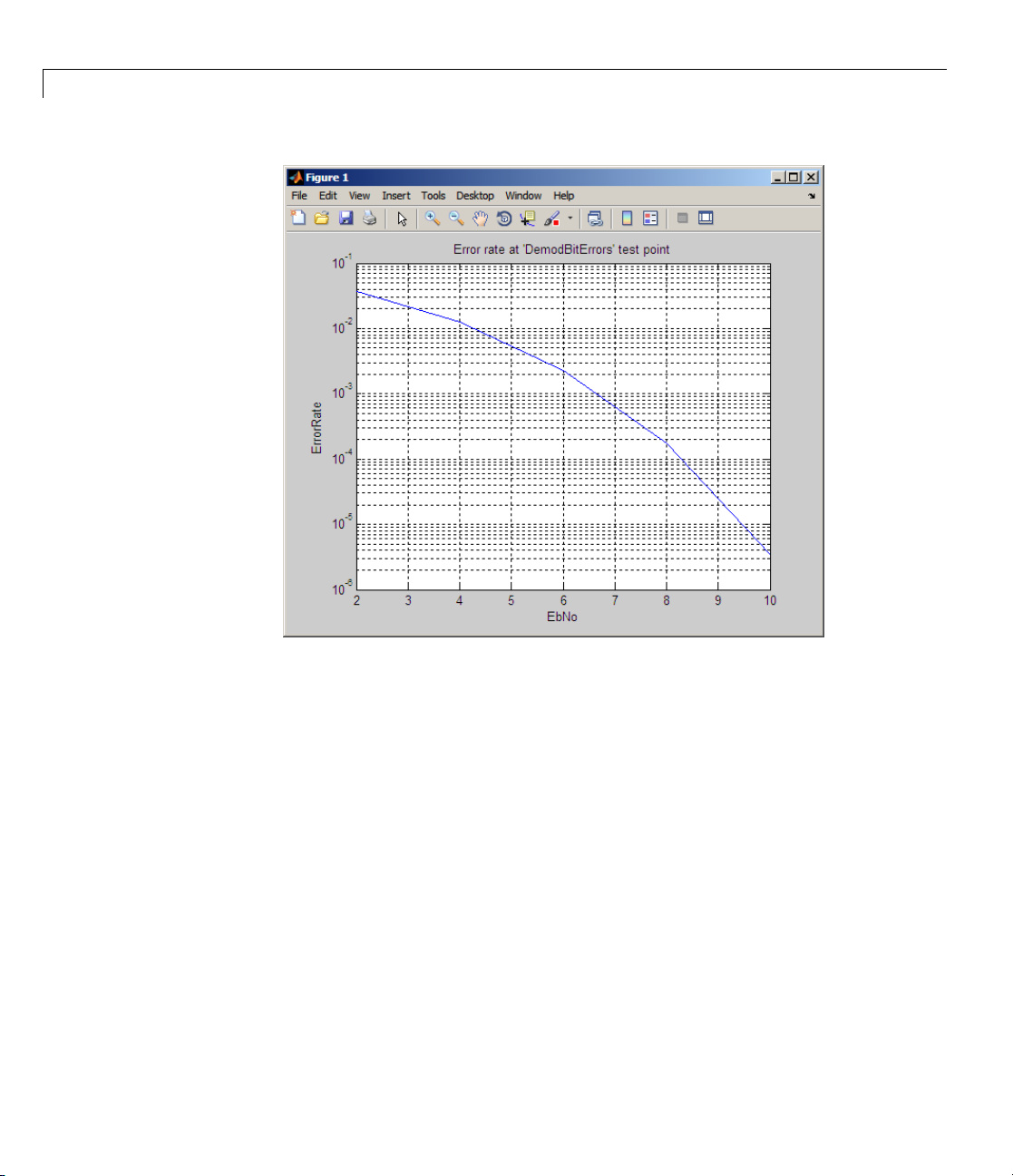
1 Gettin g Started

1-38

2 Set the TestParameter2 property to M. At the MATLAB command line,

enter:

grayRe

sults.TestParameter2 = 'M'

Previously, the simulation ran for multiple modulation order (M) values. Thex-axisdisplaysthe

TestParameter1 property of grayResults,which

contains EbNo values. Although the simulation ran for multiple M values, this run contains data for M=2.

3 Plot

multiple error rate curves by entering the following at the MATLAB

and line.

comm

semilogy(grayResults)

s script genera tes the following figure.

Thi

Running Simulations U sing the Error Rate Test Console

Running the Simulation Using Parallel Computing Toolbox Software

If you have a Parallel Computing Toolbox™ user license and you create a matlabpool, the test console runs the simulation in parallel. This approach reduces the processing time.

Note If you do not have a Parallel Computing Toolbox user license you are unable to perform this section of the tutorial.

1 If you have a Parallel Computing Toolbo x license, run the following

command to start your default matlabpool:

matlabpool

1-39

1 Gettin g Started

Ifyouhaveamulticorecomputer,then the default matlabpool uses the cores as workers.

2 Using the workers, run the simulation. At the MATLAB command line,

enter:

tic; run(testConsole); toc

MATLAB returns output similar to the following:

4 workers available for p aral lel computing. Simulations ..., will be distributed among these worke rs. Running simulations... Elapsed time is 87.449652 seconds.

Notice that the simulation runs more than three times as fast than in the previous section.

1-40

Creating a System File and Attaching It to the Test Console

In the previous sections, you used an existingGraycodedmodulatorsystem file to generate data. In this section, you create a system file and then attach it to the Error Rate Test C onsole.

This example outlines the tasks necessary for converting legacy code to a system file you can attach to the Error Rate Test Console. Use commdoc_gray as the starting point for your system file. The files you use in this section of the tutorial reside in the following folder:

matlab\help\toolbox\comm\examples

1 Copy the system basic API template, SystemBasicTemplate.m, as

MyGrayCodedModulation . m.

2 Rename the references to the system name in the file. First, rename the

system definition by changing the class name to MyGrayCodedModulation. Replace the following lines, lines 1 and 2, of the file:

classdef SystemBasicTemplate < testconsole.SystemBasicAPI

Running Simulations U sing the Error Rate Test Console

%SystemBasicTemplate Template for creating a syst em

with these lines:

classdef MyGrayCodedModulation < testconsole.SystemBasicAPI %MyGrayCodedModulation Gray coded modulation system

3 Rename the constructor by replacing:

function obj = SystemBasi cTemplate %SystemBasicTemplate Construct a system

with

function obj = MyGrayCode dModulation %MyGrayCodedModulation Construct a Gray coded mod ulat ion system

4 Enter a description for your system. Update the obj.Description

parameter with the following information:

obj.Description = 'Gray c oded modulation';

Becauseyouarenotusingthereset and setup methods for this system, leave these methods empty.

5 Copy lines 12–44 from commdoc_gray.m to the body of the run method.

6 Copy Lines 54–57 from commdoc_gray.m to the body of the ru n method.

7 Change EbNo to a test parameter. This change allows the system to obtain

EbNo values from the Error Rate Test Console. As a test parameter, EbNo becomes a variable, which allows simulations to run for different values. Locate the following line of syntax in the file:

EbNo = 10; % In dB

Replace it with:

EbNo = getTestParameter(obj,'EbNo');

8 Add modulation order, M, as a new test parameter for the simulation.

Locate the following syntax:

1-41

1 Gettin g Started

M = 16; % Size of signal constellation

Replace it with:

M = getTestParameter(obj,'M');

9 Register the test parameters to the test console.

• Declare EbNo as a test parameter by placing the following line of code in

the body of the

registerTestParameter(obj,'EbNo',0,[-50 50]);

The parameter defaults to 0 dB and can take values between -50 dB and 50 dB.

• Declare M as a test parameter by placing the following line of code in

the body of the

registerTestParameter(obj,'M',16,[2 1024]);

1-42

The parameter defaults to 16 QAM Modulation and can take values from 2 through 1024.

10 AddEbNoandMtothetestparameterslistinthe

MyGrayCodedModulationF ile file.

% Test Parameters

properties

EbNo = 0;

M=16;

end

This adds EbNo and M to the possible test parameters list. EbNo defaults to a value of 0 dB. M defaults to a value of 16.

11 Define test probe locations in the run method. In this example, you are

calculating end-to-end error rate. This calculation requires transmitted bitsandreceivedbits. Addoneprobefor obtaining transmitted bits and one probe for received bits.

• Locate the random binary data stream creation code by searching for

the following lines:

Running Simulations U sing the Error Rate Test Console

% Create a binary data stream as a column vector.

x = randi([0 1],n,1); % Random binary data stream

• Add a probe, TxBits, after the random binary data stream creation:

% Create a binary data stream as a column vector. x = randi([0 1],n,1); % Random binary data stream setTestProbeData(obj,'TxBits',x);

This code sends the random binary data stream, x,totheprobeTxBits.

• Locate the demodulation code by searching for the following lines:

% Demodulate signal using 16-QAM. z = demodulate(hDemod,yRx);

• Add a probe, RxBits, after the demodulation code.

% Demodulate signal using 16-QAM. z = demodulate(hDemod,yRx); setTestProbeData(obj,'RxBits',z);

This code sends the binary received data stream, z,totheprobeRxBits.

12 Register the test probes to the Error Rate Test Console, making it

possible to obtain data from the system. Add these probes to the function

function register(obj) % REGISTER Register the sy ste m with a test console % REGISTER(H) registers te st parameters and test probes of the % system, H, with a test console.

registerTestParameter(obj,'EbNo',0,[-50 50]);

registerTestParameter(obj,'M',16,[2 1024]);

registerTestProbe(obj,'TxBits') registerTestProbe(obj,'RxBits')

end

13 Save the file. The file is ready for use with the system.

1-43

1 Gettin g Started

14 Create a Gray coded modulation system. At the MATLAB command line,

enter:

mySystem = MyGrayCodedModulation

MATLAB returns the following output:

mySystem =

Description: 'Gray coded modulation'

EbNo: 0

M: 16

15 Create an Error Rate Test Console by entering the following at the

MATLAB command line:

testConsole = commtest.ErrorRate

TheMATLABsoftwarereturnsthefollowingoutput:

1-44

testConsole =

Description: 'Error Rate T est Console'

SystemUnderTestName: 'commtest.MPSKSystem'

FrameLength: 500

IterationMode: 'Combinatorial'

SystemResetMode: 'Reset at new simu lation point'

SimulationLimitOption: 'Number of transmissions'

TransmissionCountTestPoint: 'Not set'

MaxNumTransmissions: 1000

16 Attach the system file MyGrayCodedModulation to the error rate test

console by entering the following at the MATLAB command line:

attachSystem(testConsole, mySystem)

Running Simulations U sing the Error Rate Test Console

Configuring the Error Rate Test Console and Running aSimulation

Configure the Error R ate Test Console to obtain error rate metrics from the attached sys tem. The Error Rate Test Console defines metrics as number of errors, number of transmissions, and error rate.

1 At the MATLAB command line, enter:

registerTestPoint(testConsole, 'DemodBitErrors', 'TxBits', 'RxBits');

This line defines the test point, DemodBitErrors, and compares bits from theTxBitsprobetothebitsfromtheRxBitsprobe. TheErrorRateTest Console calculated metrics for this test point.

2 Configure the Error Rate Test Console to run simulations for EbNo values.

Start at 2 dB and end at 10 dB, with a step size of 2 dB and M values of 2, 4, 8, and 16. At the MATLAB command line, enter:

setTestParameterSweepValues(testConsole, 'EbNo', 2:2:10) setTestParameterSweepValues(testConsole, 'M', [2 4 8 16])

3 Set the simulation limit to the number of transmissions.

testConsole.SimulationLimitOption = 'Number of transmissions'

4 Set the maximum number of transmissions to 1000.

testConsole.MaxNumTransmissions = 1000

5 Configure the Error Rate Test Console so it uses the demodulator bit error

test point for determining the number of transmitted bits.

testConsole.TransmissionCountTestPoint = 'DemodBitErrors'

6 Run the simulation. At the MATLAB command line, enter:

run(testConsole)

7 Obtain the results of the simulation. At the MATLAB command line, enter:

grayResults = getResults(testConsole)

1-45

1 Gettin g Started

8 To obtain more accurate results, run the simulations for a given minimum

number of errors. In this example, you also limit the number of simulation bits so that the simulations do not run indefinitely. At the MATLAB command line, enter:

testConsole.SimulationLimitOption = 'Number of errors or transmissions'; testConsole.MinNumErrors = 100; testConsole.ErrorCountTestPoint = 'DemodBitErrors'; testConsole.MaxNumTransmissions = 1e8; testConsole

9 Run the simulation by entering the following at the MATLAB command

line.

run(testConsole);

10 Generate the new results in a Figure window by entering the following at

the MATLAB command line.

1-46

grayResults = getResults(testConsole); grayResults.TestParameter2 = 'M' semilogy(grayResults)

This script g enerates the foll owing figure.

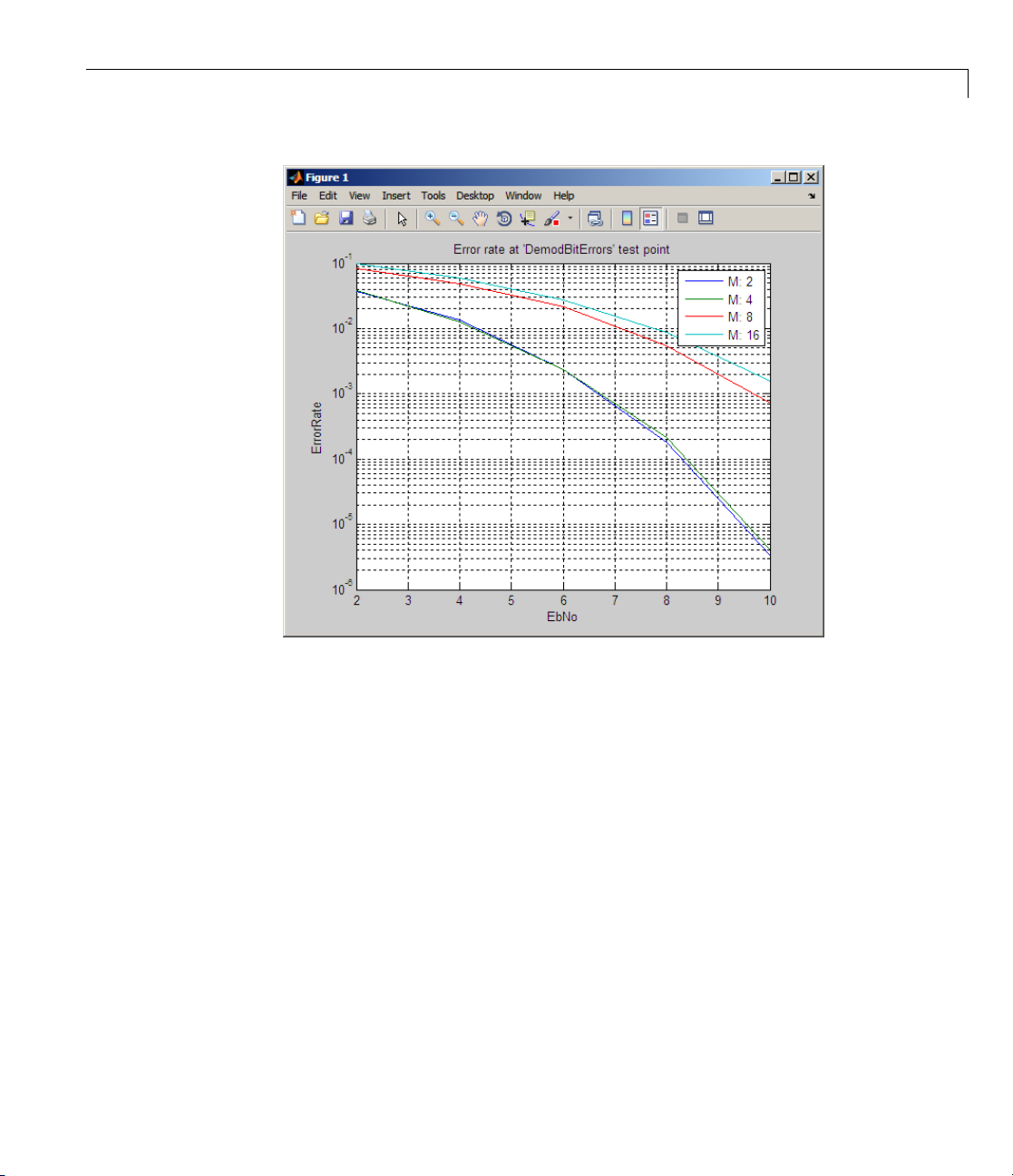
Running Simulations U sing the Error Rate Test Console

Optimizing Your System for Faster Simulations

In the previous example, the system only utilizes the run method. Every time the object calls the the object sets the M and SNR values. This time interval includes: obtaining numbers from the test console, calculating intermediate values, and setting other variables.

In contrast, the system basic API provides a Rate Test Console configures the system once for each simulation point. This change relieves the parameters, thus reducing simulation time.

The

run method o f a system also creates a new modulator (hMod) and a new

demodulator (hDemod). Creating a modulator or a demodulator is much more time consuming than just modifying a property of these objects. Create a modulator and a demodulator object once when the system is constructed.

run method, which is every 3e4 bits for this simulation,

setup method where the Error

run method from getting and setting simulation

1-47

1 Gettin g Started

Then, modify its properties in the setup method of the system to speed up the simulations.

1 SavethefileMyGrayCodedModulationas

MyGrayCodedModulationOptimized .

2 In the MyG rayC odedModulationO ptimi zed file, replace the constructor

name and the class definition name.

• Locate the following lines of code:

classdef MyGrayCodedModulation < testconsole.SystemBasicAPI %MyGrayCodedModulation Gray coded modulation system

• Replace them with:

classdef MyGrayCodedModulationOptimized < testconsole.SystemBasicAPI %MyGrayCodedModulationOptimized Gray coded modulation system

3 In the MyGrayC odedModulationOptimized ﬁle, replace the constructor

name.

1-48

• Locate the following lines of code:

function obj = MyGrayCode dModulation %MyGrayCodedModulation Construct a Gray coded mod ulat ion system

• Replace them with:

function obj = MyGrayCode dModulationOptimized %MyGrayCodedModulationOptimized Construct a Gray %coded modulation system

4 Move the overs am pling rate definition from the run method to the setup

method.

nSamp = 1; % Oversampling rate

5 Move code r

from the

elated to setting M to the

method and paste to the setup method.

M = getTestParameter(obj,'M'); k = log2(M); % Number of bits per symbol

setup method. Cut the following lines

Running Simulations U sing the Error Rate Test Console

6 In the setup method, replace M with the object property M.

obj.M = getTestParameter(obj,'M'); k = log2(obj.M); % Number of bits per symbol

This change provides access to the M value from the run method.

7 Move code related to setting EbNo to the setup method. Cut the following

lines from the

EbNo = getTestParameter(obj,'EbNo');

SNR = EbNo + 10*log10(k) - 10*log10(nSamp);

8 In the setup method, replace EbNo with the object property EbNo. T his

run method and paste to the setup method.

change provides access to the EbNo value from the run method.

obj.EbNo = getTestParameter(obj,'EbNo'); SNR = obj.EbNo + 10*log10(k) - 10*log10(nSamp);

9 Create a new internal variable called SNR to store the calculated SNR

value. Define the SNR property as a private property; it is not a test parameter. With this change, the system calculates SNR in the

setup

method and accesses it from the run method. Add the following lines of code the system file, after the Test Parameters block.

%=================================================================

% Internal variables properties (Access = private)

SNR

end

10 In the setup method, replace SNR with object property SNR.

obj.SNR = obj.EbNo + 10* log1 0(k) - 10*log10(nSamp);

11 In the run method, replace M with obj.M and SN R with obj.SNR.

hMod = modem.qammod(obj.M); % Create a -QAM modulator yNoisy = awgn(yTx,obj.SNR,'measured');

1-49

1 Gettin g Started

Notice that the run method creates the QAM modulator and demodulator.

12 Move the QAM modulator and demodulator creation out of the run method.

Move following lines from the

run method to the constructor (i.e the m e thod

named MyGrayCodedModulationOptimized)

%% Create Modulator and D emod ulator hMod = modem.qammod(obj.M); % Create a 16-QAM modulator hMod.InputType = 'Bit'; % Accept bits as inputs hMod.SymbolOrder = 'Gray'; % Accept bits as inputs hDemod = modem.qamdemod(hMod); % Create a 16-QAM based on

% the modulator

13 Create private properties called Modulator and Demodulator to store the

modulator and demodulator objects.

% Internal variables properties (Access = priva te) SNR Modulator Demodulator end

1-50

14 In the constructor method, replace hMod and hDemod with the object

property

15 In the run method, replace hMod and hDemod with o bject properties

obj.Modulator and obj.Demodulator.

16 Locate the setup region of the ﬁle.

obj.Modulator and obj.Demodulator respectively.

obj.Modulator = modem.qammod(obj.M); % Create a 16-QAM modulator obj.Modulator.InputType = 'Bit'; % Accept bits as inputs obj.Modulator.SymbolOrder = 'Gray'; % A ccept bits as inputs obj.Demodulator = modem.qamdemod(obj.Modulator);

y = modulate(obj.Modulator,x); z = demodulate(obj.Demodulator,yRx);

function setup(obj) % SETUP Initialize the sys tem

Running Simulations U sing the Error Rate Test Console

% SETUP(H) gets current te st parameter value(s) from the test % console and initializes system, H, accordingly.

17 Set the M value of the modulator and demodulator by adding the following

lines of code to the setup.

obj.Modulator.M = obj.M; obj.Demodulator.M = obj.M;

18 Save the ﬁle.

19 Create an optimized system. At the MATLAB command line, enter:

myOptimSystem = MyGrayCodedModulationOptimized

20 Create an Error Rate Test Console and attach the system to the test

console. At the MAT LAB command line, type:

testConsole = commtest.ErrorRate(myOptimSystem)

21 At the MATLAB command line, type:

registerTestPoint(testConsole, 'DemodBitErrors', 'TxBits', 'RxBits');

This line defines the test point, DemodBitErrors, and compares bits from theTxBitsprobetothebitsfromtheRxBitsprobe. TheErrorRateTest Console calculated metrics for this test point.

22 Configure the Error Rate Test Console to run simulations for EbNo values.

Start at 2 dB and end at 10 dB, with a step size of 2 dB and M values of 2, 4, 8, and 16. At the MATLAB command line, type:

setTestParameterSweepValues(testConsole, 'EbNo', 2:2:10) setTestParameterSweepValues(testConsole, 'M', [2 4 8 16])

23 Configure the Error Rate Test Console so it uses the demodulator bit error

test point for determining the number of transmitted bits.

testConsole.TransmissionCountTestPoint = 'DemodBitErrors'

1-51

1 Gettin g Started

24 To obtain more accurate results, run the simulations for a given minimum

number of errors. In this example, you also limit the number of simulation bits so that the simulations do not run indefinitely. At the MATLAB command line, type:

25 Run the simulation. At the MATLAB command line, type:

tic; run(testConsole); toc

MATLAB returns the following information:

Running simulations... Elapsed time is 240.459286 seconds.

1-52

Notice that these optimization changes reduce the simulation run time about 10%.

26 Generate the new results in a Figure window. At the MATLAB command

line, type:

grayResults = getResults(testConsole); grayResults.TestParameter2 = 'M' semilogy(grayResults)

This script g enerates the foll owing figure.

Running Simulations U sing the Error Rate Test Console

1-53

1 Gettin g Started

Learning More

In this section...

“Online Help” on page 1-54

“Demos” on page 1-54

“The MathWorks Online” on page 1-54

Online Help

To find online documentation, select Product Help from the Help menu in the MATLAB desktop. This launches the Help browser. For a more detailed explanation of any of the topics covered in this chapter, see the Communications Toolbox documentation in the left pane of the Help brow ser.

Besides this chapter, the online documentation set contains these components:

• A chapter about each of the core areas o f functionality of the toolbox (such

as error-control coding, modulation, and equalizers)

1-54

• A reference page for each function in the toolbox, indexed alphabetically

and by category

You can also use the online index of examples to find code examples that are relevant for the tasks you want to do.

Demos

To see more Communications Toolbox examples, select Demos from the Help me nu in the MATLAB desktop. This opens the Help browser to the demonstration area. Double-click Toolboxes and then select Communications to list the available demos.

The MathWorks Online

To read the Communications Toolbox documentation on the MathWorks Web site, point your Web browser to

http://www.mathworks.com/access/helpdesk/help/toolbox/comm/

Other res ources for the Communications Toolbox product are available at

http://www.mathworks.com/products/communications/

Learning More

1-55

1 Gettin g Started

1-56

Signal Sources

Every communication system has one or more signal sources. This chapter describes h ow to use Communications Toolbox to generate random signals, which are useful for simulating noise, errors, or signal sources. The sections are as follows.

• “White Gaussian Noise” on page 2-2

• “Random Symbols” on page 2-3

• “Random Integers” on page 2-4

• “Random Bit Error Patterns” on page 2-5

For more random number g enerators, see the online reference pages for the built-in MATLAB functions

rand and randn.

2 Signal Sources

White Gaussian Noise

The wgn function generates random matrices using a w hite Gaussian noise distribution. You specify the powe r of the noise in either dBW (decibels relative to a watt), dBm, or linear units. You can generate either real or complex noise.

For example, the command below generates a column vector of length 50 containing real white Gaussian noise whose power is 2 dBW. The function assumes that the load impedance is 1 ohm.

y1 = wgn(50,1,2);

To generate complex white Gaussian noise whose power is 2 watts, across a load of 60 ohms, use either of the commands below. The ordering of the string inputs does not matter.

y2 = wgn(50,1,2,60,'complex','linear'); y3 = wgn(50,1,2,60,'linear','complex');

2-2

To send a signal through an additive white Gaussian noise channel, use the

awgn function. See “AWGN Channel” on page 11-3 for more information.

Random Symbols

The randsr c function generates random matrices whose entries are chosen independently from an alphabet that you specify, with a distribution that you specify. A special case generates bipolar matrices.

For example, the command below generates a 5-by-4 matrix whose entries are independently chosen and uniformly distributed in the set {1,3,5}. (Your results might vary because these are random numbers.)

a = randsrc(5,4,[1,3,5])

Random Symbols

3515 1533 1331 1135 3113

If you want 1 to be twice as likely to occur as either 3 or 5, use the command below to prescribe the skewed distribution. The third input argument has two rows, o ne of which indicates the possible values of

b and the other indicates

the probability of each value.

b = randsrc(5,4,[1,3,5; .5,.25,.25])

3351 1111 1511 1313 3131

2-3

2 Signal Sources

Random Integers

The randint function generates random integer matrices whose entries are in a rang e that yo u specify. A special case generates random binary matrices.

For example, the command below generatesa5-by-4matrixcontaining random integers between 2 and 10.

c = randint(5,4,[2,10])

2446 45105 97108 5523

103410

If your desired range is [0,10] instead of [2,10], you can use either of the commands below . They produce different numerical results, but use the same distribution.

2-4

d = randint(5,4,[0,10]); e = randint(5,4,11);

Random Bit Error Patterns

The randerr function generates matrices w ho se entries are either 0 or 1. However, its options are different from those of is meant for testing error-control coding. For example, the command below generates a 5-by-4 binary matrix, where each row contains exactly one 1.

f = randerr(5,4)

0010 0010 0100 1000 0010

You might use such a comm and to perturb a binary code that consists of five four-bit codewords. Adding the random matrix

2) introduces exactly one error into each co dewo rd.

Random Bit Error Patterns

randint,becauseranderr

f to your code matrix (modulo

On the other hand, to perturb each codeword by in trod u cing one error with probability 0.4 and two errors with probability 0.6, use the command below instead.

% Each row has one '1' with probability 0.4, otherwise two '1's g = randerr(5,4,[1,2; 0.4,0.6])

0110 0100 0011 1010 0110

Note The probability matrix that is the third argument of randerr affects only the number of 1s in each row, not their placement.

2-5

2 Signal Sources

As another application, you can generate an equiprobable binary 100-element column vector using any of the commands below. The three commands produce different numerical outputs, but use the same distribution.The third input arguments vary according to each function’s particular way of specifying its behavior.

binarymatrix1 = randsrc(100,1,[0 1]); % Possible values are 0,1. binarymatrix2 = randint(100,1,2); % T wo possible values binarymatrix3 = randerr(100,1,[0 1;.5 .5]); % No 1s, or one 1

2-6

Performance Evaluation

Simulating a communication system often involves analyzing its response to the noise inherent in real-world components, studying its behavior using graphical means, and determining whether the resulting performance meets standards of acceptability. The sections in this chapter are as follows.

• “Performance Results via Simulation” on page 3-2

• “Performance Results via the Semianalytic Technique” on page 3-5

• “Theoretical Performance Results” on page 3-10

• “Error Rate Plots” on page 3-14

• “Eye Diagrams” on page 3-20

• “Scatter Plots” on page 3-21

• “Adjacent Channel Power Ratio (ACPR) Measurements” on page 3-34

• “EVM Measurements” on page 3-44

• “MER Measurements” on page 3-45

• “Selected Bibliography for Performance Evaluation” on page 3-46

Because error analysis is often a component of communication system simulation, other portions of this guide provide additional examples.

3 Performance Evaluation

Performance Results via Simulation

In this section...

“Section Overview” on page 3-2

“Using Simulated Data to Compute Bit and Symbol Error Rates” on page 3-2

“Example: Computing Error Rates” on page 3-3

“Comparing Symbol Error Rate and Bit Error Rate” on page 3-4

Section Over view

One way to compute the bit error rate or symbol error rate for a communication system is to simulate the transmission of data messages and compare all messages before and after transmission. The simulation of the communication system components using Communications Toolbox is covered in other parts of this guide. This section describes how to compare the data messages that enter and leave the simulation.

3-2

Another example of computing performance results via simulation is in “Curve Fitting for Error Rate Plots” on page 3-15 in the discussion of curve fitting.

Using Simulated Data to Compute Bit and Symbol Error Rates

The biterr function compares two sets of data and computes the number of bit errors and the bit error rate. The data and computes the number of symbol errors and the symbol error rate. An error is a discrepancy between corresponding points in the two sets of data.

Of the two sets of data, typically one represents messages entering a transmitter and the other represents recovered messages leaving a receiver. You might also compare data entering and leaving other parts of your communication system, for e xample, data entering an encoder and data leaving a decoder.

If your communication system uses several bits to represent one symbol, counting bit errors is different from counting symbol errors. In e ither the bit-

symerr function compares two s ets of

Performance Results via Simulation

or symbol-counting case, the error rate is the number of errors divided by the total number (of bits or symbols) transmitted.

Note To ensure an accurate error rate, you should typically simulate enough data to produce at least 100 errors.

If the error rate is very small (for example, 10-6or smaller), the semianalytic technique might compute the result more quickly than a simulation-only approach. See “Performance Results v ia the Semianalytic Technique” on page 3-5 for more information on how to use this technique.

Example: Computing Error Rates

The script below uses the symerr function to compute the symbol error rates for a noisy linear block code. After artificially adding noise to the encoded message, it compares the resulting noisy code to the original code. Then it decodes and compares the decoded message to the original one.

m = 3; n = 2^m-1; k = n-m; % Prepare to use Hamming code. msg = randint(k*200,1,2); % 200 messa ges of k bits each code = encode(msg,n,k,'hamming'); codenoisy = rem(code+(rand(n*200,1)>.95),2); % Add noise. % Decode and correct some errors. newmsg = decode(codenoisy,n,k,'hamming'); % Compute and display symbol error rates. [codenum,coderate] = symerr(code,codenoisy); [msgnum,msgrate] = symerr(msg,newmsg); disp(['Error rate in the received code: ',num2str(coderate)]) disp(['Error rate after de coding: ',num2str(msgrate)])

The output is below. The error rate decreases after decoding because the Hamming decoder corrects some of the errors. Your results might vary because this example uses random numbers.

Error rate in the received code: 0.054286 Error rate after decoding: 0.03

3-3

3 Performance Evaluation

Comparing Symbo

In the example ab each symbol is a b symbol errors a

a = [1 2 3]'; b = [1 4 4]'; format rat % Display fractions instead of decimals. [snum,srate] = symerr(a,b) [bnum,brate] = biterr(a,b)

The output is

snum =

srate =

2/3

bnum =

ove, the symbol errors and bit errors are the same because

it. The commands below illustrate the difference between

nd bit errors in other situations.

below.

l Error Rate and Bit Error Rate

3-4

brate =

5/9

is 5 because the second entries differ in two bits and the third entries

bnum

er in three bits.

diff

l number of bits is, by definition, the number of entries in

tota

mum number of bits among all entries of

maxi

brate is 5/9 because the total number of bits is 9. The

a or b times the

a and b.

Performance Results via the Semianalytic Technique

In this section...

“Section Overview” on page 3-5

“When to Use the Semianalytic Technique” on page 3-5

“Procedure for the Semianalytic Technique” on page 3-6

“Example: Using the Semianaly tic Technique” on page 3-7

Section Over view

The technique described in “Performance Results via Simulation” on page 3-2 works well for a large v ariety of communication systems, but can be prohibitively time-consuming if the system’s error rate is very small (for example, 10 technique as an a lternative way to compute error rates. For certain types of systems, the semianalytic technique can produce results much more quickly than a nonanalytic method that uses only simulated data.

-6

or smaller). This section describes how to use the semianalytic

The semianalytic technique uses a combination of simulation and analysis to determine the error rate of a communication system. The function in Communications Toolbox helps you implement the semianalytic technique by performingsomeoftheanalysis.

For more background information on the semianalytic technique, refer to [3].

semianalytic

When to Use the Semianalytic Technique

The semianalytic technique works well for certain types of communication systems, but not for others. The semianalytic technique is applicable if a system has all of these characteristics:

• Any effects of multipath fading, quantization, and amplifier nonlinearities

must precede the effects of noise in the actual channel being modeled.

• The receiver is perfectly synchronized with the carrier, and timing jitter is

negligible. Because phase noise and timing jitter are slow processes, they reduce the applicability of the semianalytic technique to a communication system.

3-5

3 Performance Evaluation

• The noiseless simulation has no errors in the received signal constellation.

Distortions from sources other than noise should be mild enough to keep each signal point in its correct decision region. If this is not the case, the calculated BER is too low. For instance, if the modeled system has a phase rotation that places the received signal points outside their proper decision regions, the semianalytic technique is not suitable to predict system performance.

Furthermore, the

semianalytic function assumes that the noise in the

actual channel being modeled is Gaussian. For details on how to adapt the semianalytic technique for non-Gaussian noise, see the discussion of generalized exponential distributions in [3].

Procedure for the Semianalytic Technique

The procedure below describes how you would typically implem e nt the semianalytic technique using the

1 Generate a message signal containing at least M

the alphabet size of the modulation and L is the length of the impulse response of the channel in symbols. A common approach is to start with an augmented binary pseudonoise (PN) sequence of total length augmented PN sequence is a PN sequence with an extra zero appended, which makes the distribution of ones and zeros equal.

2 Modulate a carrier with the message signal using baseband modulation.

Supported modulation types are listed on the reference page for

semianalytic. Shape the resultant signal with rectangular pulse shaping,

using the oversampling factor that you will later use to filter the modulated signal. S tore the result of this step as

3 Filter the modulated signal with a transmit filter. This filter is often a

square-root raised cosine filter, but you can also use a Butterworth, Bessel, Chebyshev type 1 or 2, elliptic, or more general FIR or IIR filter. If you use a square-root raised cosine filter, use it on the nonoversampled modulated signal and specify the oversampling factor in the filtering function. If you use another filter type, you can apply it to the rectangularly pulse shaped signal.

semianalytic function:

symbols, where M is

txsig for later use.

(log2M)M

.An

3-6

Performance Results via the Semianalytic Technique

4 Run the filtered signal through a noiseless channel. This channel can

include multipath fading effects, phase shifts, amplifier nonlinearities, quantization,andadditionalfiltering,butitmustnotincludenoise.Store the result of this step as

5 Invoke the semianalytic function using the txsig and rxsig data from

rxsig for later use.

earlier steps. Specify a receive filter as a pair of input arguments, unless you want to use the function’s default filter. The function filters

rxsig

and then determines the error probability of each received signal point by analytically applying the Gaussian noise distribution to each point. The function averages the error probabilities over the entire received signal to determine t he overall error probability. If the error probability calculated in this way is a symbol error probability, the function converts it to a bit error rate, typically by assuming Gray coding. The function returns the bit error rate (or, in the case of DQPSK modulation, an upper b ound on the bit error rate).

Example: Using the Semianalytic Technique

The example below illustrates the procedure described above, using 16-QAM modulation. It also compares the error rates obtained from the semianalytic technique w ith the theoretical error rates obtained from published formulas and computed using the the error rates obtained using the two methods are nearly identical. The discrepancies between the theoretical and computed error rates are largely due to the phase offset in this example’s channel model.

berawgn function. The resulting plot shows that

% Step 1. Generate message signal of length >= M^L. M = 16; % Alphabet size of modulation L = 1; % Length of impulse response of channel msg = [0:M-1 0]; % M-ary message sequence of length > M^L

% Step 2. Modulate the message signal using baseband modulation. modsig = qammod(msg,M); % Use 16-QAM. Nsamp = 16; modsig = rectpulse(modsig,Nsamp); % Use rectangular pulse shapin g.

% Step 3. Apply a transmit filter. txsig = modsig; % No filter in this example

% Step 4. Run txsig through a noiseless channel.

3-7

3 Performance Evaluation

rxsig = txsig*exp(1i*pi/180); % Static phase offset of 1 degree % Step 5. Use the semianalytic function. % Specify the receive filter as a pair of input arguments. % In this case, num and den describe an ideal integrator. num = ones(Nsamp,1)/Nsamp; den = 1; EbNo = 0:20; % Range of Eb/No values under study ber = semianalytic(txsig,rxsig,'qam',M,Nsamp,num,den,EbNo );

% For comparison, calculate theoretical BER. bertheory = berawgn(EbNo,'qam',M);

% Plot computed BER and theoretical BER. figure; semilogy(EbNo,ber,'k*'); hold on; semilogy(EbNo,bertheory,'ro'); title('Semianalytic BER Compared with Theoretical BER'); legend('Semianalytic BER with Phase O ffset',...

'Theoretical BER Without P hase Offset','Location','SouthWest');

hold off;

3-8

This example creates a figure like the one below.

Performance Results via the Semianalytic Technique

3-9

3 Performance Evaluation

Theoretical Performance Results

In this section...

“Computing Theoretical Error Statistics” on page 3-10

“Plotting Theoretical Error Rates” on page 3-10

“Comparing Theoretical and Empirical Error Rates” on page 3-11

Computing Theoretical Error Statistics

While the biterr function discussed above can help you gather e m pirical error statistics, you might also compare those results to theoretical error statistics. Certain types of communication systems are associated with closed-form expressions for the bit error rate or a bound on it. The functions listed in the table below compute the closed-form expressions for some types of communication systems, where such expressions exist.

Type of Communication System

Uncoded AWGN channel

Coded AWGN channel

Uncoded Rayleigh and Rician fading channel

Uncoded AWGN channel with imperfect synchronization

Each function’s reference page lists one or more books containing the closed-form expressions that the function implements.

Function

berawgn

bercoding

berfading

bersync

Plotting Theoretical Error Rates

The example below uses the bercoding function to compute upper bounds on bit error rates for convolutional coding with a soft-decision decoder. The data used for the generator and distance spectrum are from [5] and [2], respectively.

coderate = 1/4; % Code rate

3-10

Theoretical Performance Results

% Create a structure dspec with information about distance spectrum. dspec.dfree = 10; % Minimum free distance of code dspec.weight = [1 0 4 0 12 0 32 0 80 0 192 0 44 8 0 1024 ...

0 2304 0 5120 0]; % Distance spectrum of code EbNo = 3:0.5:8; berbound = bercoding(EbNo,'conv','soft',coderate,dspec); semilogy(EbNo,berbound) % Plot the re sults. xlabel('E_b/N_0 (dB)'); ylabel('Upper Bound on BE R'); title('Theoretical Bound on BER for Convolutional Coding'); grid on;

This example produces the following plot.

Comparing Theoretical and Empirical Error Rates

The example below uses the berawgn function to compute symbol error rates for pulse amplitude modulation (PAM) with a series of E comparison, the code simulates 8-PAM with an AWGN channel and computes empirical symbol error rates. The code also plots the theoretical and empirical symbol error rates on the same set of ax es.

% 1. Compute theoretical error rate using BERAWGN. M = 8; EbNo = [0:13]; [ber, ser] = berawgn(EbNo, 'pam',M);

values. For

b/N0

3-11

3 Performance Evaluation

% Plot theoretical results. figure; semilogy(EbNo,ser,'r'); xlabel('E_b/N_0 (dB)'); ylabel('Symbol Error Rate'); grid on; drawnow;

% 2. Compute empirical error rate by simulating. %Setup. n = 10000; % Number of symbols to process k = log2(M); % Number of bits per symbol % Convert from EbNo to SNR. % Note: Because No = 2*noiseVariance^ 2, we must add 3 dB % to get SNR. For details, see Proakis book listed in % "Selected Bibliography for Performance Evaluation." snr = EbNo+3+10*log10(k); ynoisy=zeros(n,length(snr)); % Preallocate to save time.

% Main steps in the simulation x = randint(n,1,M); % Crea te message signal. y = pammod(x,M); % Modulat e. % Send modulated signal th rou gh AWGN channel. % Loop over different SNR values. for jj = 1:length(snr)

ynoisy(:,jj) = awgn(real(y),snr(jj),'measured'); end z = pamdemod(ynoisy,M); % Demodulate.

3-12

% Compute symbol error rat e from simulation. [num,rt] = symerr(x,z);

% 3. Plot empirical results, in same figure. hold on; semilogy(EbNo,rt,'b.'); legend('Theoretical SER','Empirical SER'); title('Comparing Theoretical and Empirical Error Rates'); hold off;

This example produces a plot like the one in the following figure. Your plot might vary because the simulation uses random numbers.

Theoretical Performance Results

3-13

3 Performance Evaluation

Error Rate Plots

In this section...

“Section Overview” on page 3-14

“Creating Error Rate Plots Using semilogy”onpage3-14

“Curve Fitting for Error Rate Plots” on p age 3-15

“Example: Curve Fitting for an Error Rate Plot” on page 3-15

Section Over view

Errorrateplotsprovideavisualwaytoexaminetheperformanceofa communication system, and they are often included in publications. This section mentions som e of the tools you can use to create error rate plots, modify them to suit your needs, and do curve fitting on error rate data. It also provides an example of curve fitting. For more detailed discussions about the more general plotting capabilities in MATLAB, see the MATLAB documentation set.

3-14

Creating Error Rate Plots Using semilogy

In many error rate plots, the horizontal axis indicates Eb/N0values in dB and the vertical axis indicates the error rate using a logarithmic (base 10) scale. To see an example of such a plot, as well as the code that creates it, see “Comparing Theoretical and Empirical Error Rates” on page 3-11. The part of that example that creates the plot uses the logarithmic scale on the vertical axis and a linear scale on the horizontal axis.

Other examples that illustrate the use o f

• “Example: Using the Semianalytic Technique” on page 3-7, which also

illustrates

semilogy function to produce a

semilogy are in these sections:

- Plotting two sets of data on one pair of axes

- Adding a title

- Adding a legend

• “Plotting Theoretical Error Rates” onpage3-10,whichalsoillustrates

Error Rate Plots

- Adding axis labels

- Addi ng grid line s

Curve Fitting for Error Rate Plots

Curve fitting is useful when you have a small or imperfect data set but want to plot a smooth curve for presentation purposes. The Communications Toolbox offers curve-fitting capabilities that are well suited to the situation when the empirical data describes error rates at different E

values. This function enables you to

b/N0

• Customize various relevant aspects of the curve-fitting process, such as the

type of closed-form function (from a list of preset choices) used to generate the fit.

berfit function in

• Plot empirical data along with a curve that

• Interpolate points on the fitted curve between E

empirical data set to make the plot smoother looking.

• Collect relevant information about the fit, such as the numerical values of

points along the fitted curve and the coefficients of the fit expression.

Note The berfit function is intended for curve fitting or interpolation, not extrapolation. Extrapolating BER data beyond an order of m agnitude below the s mallest empirical BER value is inherently unreliable.

For a full list of inputs and outputs for berfit, see its reference page.

berfit fits to the data.

values in your

b/N0

Example: Curve Fitting for an Error Rate Plot

This example simulates a simple DBPSK (differential binary phase shift keying) co mmunicatio n system and plots error rate data for a series of E values. It uses the berfit function to fit a curve to the somewhat rough set of empirical error rates. Because the example is long, this discussion presents it in multiple steps:

• “Setting Up Parameters for the Simulation” on page 3-16

b/N0

• “Simulating the System Using a Loop” on page 3-16

3-15

3 Performance Evaluation

• “Plotting the Empirical Results and the Fitted Curve” on page 3-18

Setting Up Parameters for the Simulation

Thefirststepintheexamplesetsuptheparameterstobeusedduringthe simulation. Parameters include the range of E minimum number of errors that must occur before the simulation computes an error rate for that E

b/N0

value.

Note For most applications, you should base an error rate computation on a larger number of errors than is used here (for instance, you might change

numerrmin to 100 in the code below). However, this example uses a small

number of errors merely to illustrate ho w curve fitting can smooth ou t a rough data set.

% Set up initial parameters. siglen = 100000; % Number of bits in each trial M = 2; % DBPSK is binary. hMod = modem.dpskmod('M', M); % Creat e a DPSK modulator hDemod = modem.dpskdemod(hMod); % Create a DPSK

% demodulator using the mo dula tor object EbNomin = 0; EbNomax = 9; % EbNo range, in dB numerrmin = 5; % Compute BER only after 5 errors occur. EbNovec = EbNomin:1:EbNomax; % Vector of EbNo values numEbNos = length(EbNovec); % Number of EbNo values % Preallocate space for certain data. ber = zeros(1,numEbNos); % BER values intv = cell(1,numEbNos); % Cell array of confidence intervals

values to consider and the

b/N0

3-16

Simulating the System Using a Loop

Thenextstepintheexampleistouseafor loop to vary the Eb/N0value (denoted by each value. The inner agiven has occurred. When the system is very noisy, this requires only one pass through the

EbNo in the code) and simulate the communication system for

while loop ensures that the simulation continues to use

EbNo value until at least the predefined minimum number of errors

while loop, but in other cases, this requires multiple passes.

Mathworks COMMUNICATIONS TOOLBOX 4 user guide

Specifications and Main Features

Frequently Asked Questions

User Manual

Getting Started

Product Overview

Section Over view

Expected Background

For New Users

For Experienced Users

Studying Components of a Communication System

Section Over view

Modulating a Random Signal

Solution of Problem

Plotting Signal Constellations

Solution of Problem

Examining the Plot

Solution of Problem

Solution of Problem

More About Delays

Simulating a Communication System

Section Over view

Using B ERTool to Run Simulations

Solution of Problem

Comparing with Theoretical Results

More About the Simulation Structure

Varying Parameters and Managing a Set of Simulations

Solution of Problem

Running Simulations U sing the Error Rate Test Console

Loading the Error Rate Test Console

Running the Simulation and Obtaining Results

Generating an Error Rate Results Figure Window

Running the Simulation Using Parallel Computing Toolbox Software

Creating a System File and Attaching It to the Test Console

Configuring the Error Rate Test Console and Running aSimulation

Optimizing Your System for Faster Simulations

Learning More

Online Help

Demos

The MathWorks Online

Signal Sources

White Gaussian Noise

Random Symbols

Random Integers

Random Bit Error Patterns

Performance Evaluation

Performance Results via Simulation

Section Over view

Using Simulated Data to Compute Bit and Symbol Error Rates

Example: Computing Error Rates

Performance Results via the Semianalytic Technique

Section Over view

When to Use the Semianalytic Technique

Procedure for the Semianalytic Technique

Example: Using the Semianalytic Technique

Theoretical Performance Results

Computing Theoretical Error Statistics

Plotting Theoretical Error Rates

Comparing Theoretical and Empirical Error Rates

Error Rate Plots

Section Over view

Creating Error Rate Plots Using semilogy

Curve Fitting for Error Rate Plots

Example: Curve Fitting for an Error Rate Plot

Setting Up Parameters for the Simulation

Simulating the System Using a Loop