Mathworks AEROSPACE TOOLBOX 2 user guide

Aerospace Toolbox

User’s Guide

How to Contact The MathWorks

www.mathworks. comp.soft-sys.matlab Newsgroup www.mathworks.com/contact_TS.html T echnical Support

suggest@mathworks.com Product enhancement suggestions bugs@mathwo doc@mathworks.com Documentation error reports service@mathworks.com Order status, license renewals, passcodes info@mathwo

com

rks.com

Web

Bug reports

Sales, prici

ng, and general information

508-647-7000 (Phone)

508-647-7001 (Fax)

The MathWorks, Inc. 3 Apple Hill Drive Natick, MA 01760-2098

For contact information about worldwide offices, see the MathWorks Web site.

Aerospace Toolbox User’s Guide

The software described in this document is furnished under a license agreement. The software may be used or copied only under the terms of the license agreement. No part of this manual may be photocopied or reproduced in any form without prior written consent from The MathW orks, Inc.

FEDERAL ACQUISITION: This provision applies to all acquisitions of the Program and Documentation by, for, or through the federal government of the United States. By accepting delivery of the Program or Documentation, the government hereby agrees that this software or documentation qualifies as commercial computer software or commercial computer software documentation as such terms are used or defined in FAR 12.212, DFARS Part 227.72, and DFARS 252.227-7014. Accordingly, the terms and conditions of this Agreement and only those rights specified in this Agreement, shall pertain to and govern theuse,modification,reproduction,release,performance,display,anddisclosureoftheProgramand Documentation by the federal government (or other entity acquiring for or through the federal government) and shall supersede any conflicting contractual terms or conditions. If this License fails to meet the government’s needs or is inconsistent in any respect with federal procurement law, the government agrees to return the Program and Docu mentation, unused, to The MathWorks, Inc.

Trademarks

MATLAB and Simulink are registered trademarks of The MathWorks, Inc. See

www.mathworks.com/trademarks for a list of additional trademarks. Other product or brand

names may be trademarks or registered trademarks of their respective holders.

Patents

The MathWorks products are protected by one or more U.S. patents. Please see

www.mathworks.com/patents for more information.

Revision History

September 2006 Online only New for Version 1.0 (Release 2006b) March 2007 Online only Revised for Version 1.1 (Release 2007a) September 2007 First printing Revised for Version 2.0 (Release 2007b) March 2008 Online only Revised for Version 2.1 (Release 2008a) October 2008 Online only Revised for Version 2.2 (Release 2008b) March 2009 Online only Revised for Version 2.3 (Release 2009a) September 2009 Online only Revised for Version 2.4 (Release 2009b) March 2010 Online only Revised for Version 2.5 (Release 2010a)

Getting Started

Product Overview ................................. 1-2

Contents

Getting Started

• “Product Overview” on page 1-2

• “Related Products” on page 1-4

• “Getting Online Help” on page 1-5

1 Getting Started

Product Overview

The Aerospace Toolbox product extends the MATL AB®technical computing environment by providing reference standards, environment models, and aerodynamic coefficient importing for performing advanced aerospace analysis to develop and evaluate your designs. The toolbox provides the following to enable you to visualize flight data in a three-dimensional environment and reconstruct behavioral anomalies in flight-test results:

• Aero.Animation, Aero.Body, Aero.Camera, and Aero.Geometry objects and

• An interface to the FlightGear flight simulator

• AninterfacetotheSimulink

To ensure design consistency, the Aerospace Toolbox software provides utilities for unit conversions, coordinate transformations, and quaternion math, as well as standards-based environmental models for the atmosphere, gravity, and magnetic fields. You can import aerodynamic coefficients directly from the U.S. Air Force Digital Data Compendium (DATCOM) to carry out preliminary control design and vehicle performance analysis.

associated methods

3D Animation™ software

1-2

The toolbox provides you with the following main features:

• Provides standards-based environmen ta l models for atmosphere, gravity,

and magnetic fields.

• Converts units and transforms coordinate systems and spatial

representations.

• Implements predefined utilities for aerospace parameter calcu lat io ns, tim e

calculations, and quaternion math.

• Imports aerodynamic coefficients directly from DATCOM.

• Interfaces to the FlightGear flight simulator, enabling visualization of

vehicle dynamics in a three-dimensional environment.

Product Overview

The Aerospace Toolbox functions can be used in applications such as aircraft technology, telemetry data reduction, flig ht control analysis, navigation analysis, visualization for flight simulation, and environmental modeling, and can help you perform the following tasks:

• Analyze, initialize, and visualize a broad range of large aerospace system

architectures, including aircraft, missiles, spacecraft (probes, satellites, manned and unmanned), and propulsion systems (engines and rockets), while reducing development time.

• Support and define new requirem ents for a ero space systems.

• Perform complex calculations and analyze data to optimize and implement

your designs.

• Test the performance of flight tests.

The Aerospace Toolbox software main tains and updates the algorithms, tables, and standard environmental models, eliminating the need to provide internal maintenance and verification of the models and reducing the cost of internal software maintenance.

1-3

1 Getting Started

Related Products

The Aerospace Toolbox software requires the MATLAB software.

In addition to Aerospace Toolbox, the Aerospace product family includes the Aerospace Blockset product. The toolbox provides s tatic data analysis capabilities, while blockset provides an environment for dynamic modeling and vehicle component modeling and simulation. The Aerospace Blockset™ software uses part of the functionality of the toolbox as an engine. Use these products together to model aerospace systems in the MATLAB and Simulink environments.

Other related products are listed in the Aerospace Toolbox product page at the MathWorks Web site. They include toolboxes and blocksets that extend the capabilities of the MATLAB and Simulink products. These products will enhance your use of the toolbox in various applications.

For more information about any MathWorks™ software products, see either

1-4

• The online documentation for that product if it is installed

• The MathWorks Web site at

www.mathworks.com

Getting Online Help

In this section...

“Exploring the Toolbox” on page 1-5

“Using the MATLAB Help System for Documentation and Demos” on page 1-5

Exploring the Toolbox

A list of the toolbox functions is available to you by typing

help aero

You can view the code for any function by typing

type function_name

Getting Online Help

Using the MATLAB Help System for Documentation and Demos

TheMATLABHelpbrowserallowsyoutoaccessthedocumentationanddemo models for all the MATLAB and Simulink based products that you have installed. The online Help includes an online search system.

Consult the Help for Using MATLAB section of the MATLAB Desktop Tools and Development Environment documentation for more information about the MATLAB Help system.

1-5

1 Getting Started

1-6

Using Aerospace Toolbox

• “Defining Coordinate Systems” on page 2-2

• “Defining Aerospace Units” on page 2-12

• “Importing Digital D ATC OM Data” on page 2-14

• “3-D Flight Data Playback” on page 2-26

2 Using Aerospace Toolbox

Defining Coordinate Systems

In this section...

“Fundamental Coordinate System Concepts” on page 2-2

“Coordinate Systems for Modeling” on page 2-4

“Coordinate Systems for Navigation” on page 2-7

“Coordinate Systems forDisplay”onpage2-10

“References” on page 2-11

Fundamental Coordinate System Concepts

Coordinate systems a llow you to keep track of an aircraft or spacecraft’s position and orientation in space. The Aerospace Toolbox coordinate sy stems are based on these underlying concepts from geodesy, astronomy, and physics.

Definitions

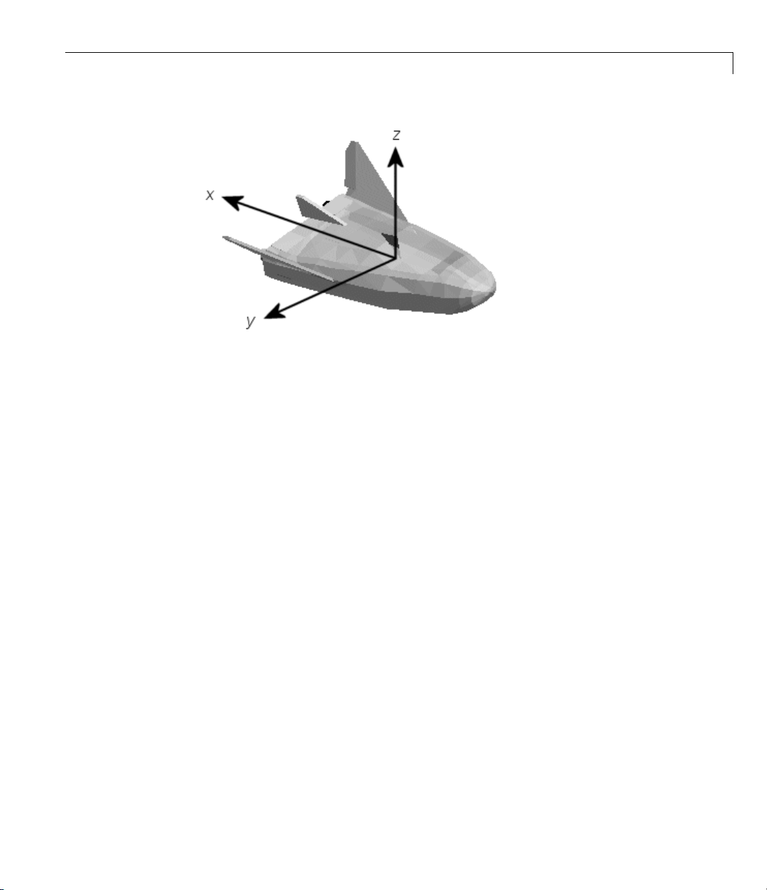
The Aerospace Toolbox software uses right-handed (RH) Cartesian coordinate systems. The right-hand rule establishes the axes.

x-y-z sequence of coordinate

2-2

An inertial frame is a nonaccelerating motion reference frame. Loosely speaking, acceleration is defined with respect to the distant cosmos. In an inertial frame, Newton’s second law (force = m ass X acceleration) holds.

Strictly defined, an inertial frame is a member of the set of all frames not accelerating relative to one another. A noninertial frame is any frame accelerating relative to an inertial frame. Its acceleration, in general, includes both translational and rotational components, resulting in pseudoforces (pseudogravity,aswellasCoriolis and centrifugal forces).

The toolbox mo dels the Earth’s shape (the geoid) as an oblate spheroid, a special type of ellipsoid with two longer axes equal (defining the equatorial plane) and a third, slightly shorter (geopolar) axis of symmetry. The equator is the intersection of the equatorial plane and the Earth’s surface. The geographic poles are the intersection o f the Earth’s surface and the geopolar axis. In general, the Earth’s geopo lar and rotation axes are not identical.

Defining Coordinate Systems

Latitudes parallel the equator. Longitudes parallel the geopolar axis. The zero longitude or prime meridian passes through Greenwich, England.

Approximations

The Aerospace Toolbox software m ak e s three standard approximations in defining coordinate systems relative to the Earth.

• The Earth’s surface or geoid is an oblate spheroid , defined by its lo nger

equatorial and shorter geopolar axes. In reality, the Earth is slightly deformed with respect to the standard geoid.

• The Earth’s rotation axis and equatorial plane are perpendicular, so that

the rotation and geopolar axes are identical. In reality, these axes are slightly misaligned, and the equatorial plane wobbles as the Earth rotates. This effect is negligible in most applications.

• The only noninertial effect in Earth-fixed coordinates is due to the Earth’s

rotation about its axis. This is a rotating, geocentric system . The toolbox ignores the Earth’s motion around the Sun, the Sun’s motion in the Galaxy, and the Galaxy’s motion through cosmos. In most applications, only the Earth’s rotation matters.

This approximation must be changed for spacecraft sent into deep space, i.e., outside the Earth-Moon system, and a heliocentric system is preferred.

Motion with Respect to Other Planets

The Aerospace Toolbox software uses the standard WGS-84 geoid to model the Earth. You can change the equatorial axis length, the flattening, and the rotation rate.

You can represent the motion of spacecraft with respect to any celestial body that is well approximated by an oblate spheroid by changing the spheroid size, flattening, and rotation rate. If the celestial body is rotating westward (retrogradely), make the rotation rate negative.

2-3

2 Using Aerospace Toolbox

Coordinate Systems for Modeling

Modeling aircraft and spacecraft is simplest if you use a coordinate system fixed in the body itself. In the case of aircraft, the forward direction is modified by the presence of wind, and the craft’s motion through the air is not the same as its motion relative to the ground.

Body Coordinates

The noninertial body coordinate system is fixed in both origin and orientation to the moving craft. The craft is assumed to be rigid.

The orientation of the body coordinateaxesisfixedintheshapeofbody.

• The

Translational Degrees of Freedom. Translations are defined by moving

along these axes by distances

Rotational Degrees of Freedom. Rotations are defined by the Euler angles

P, Q, R or Φ, Θ, Ψ.Theyare

•

x-axis points through the nose of the craft.

y-axis points to the right of the x-axis (facing in the pilot’s direction of

view), perpendicular to the

z-axis points down through the bottom of the craft, perpendicular to

the

x-y plane and satisfying the RH rule.

P or Φ: Roll about the x-axis

Q or Θ:Pitchaboutthey-axis

R or Ψ: Yaw about the z-axis

x-axis.

x, y,andz from the origin.

2-4

Defining Coordinate Systems

Wind Coordinates

The noninertial wind coordinate system has its origin fixed in the rigid aircraft. The coordinate system orientation is defined relative to the craft’s velocity V.

The o rientation of the wind coordinate axes is fixed by the velocity V.

• The

x-axis points in the direction of V.

y-axis points to the right of the x-axis (facing in the direction of V),

perpendicular to the

z-axis points perpendicular to the x-y plane in whatever way needed to

satisfy the RH rule with respect to the

x-axis.

x-andy-axes.

Translational Degrees of Freedom. Translations are defined by moving along these axes by distances

x, y,andz from the origin.

2-5

2 Using Aerospace Toolbox

Rotational Degrees of Freedom. Rotations are defined by the Euler

angles Φ, γ, χ.Theyare

• Φ: Bank angle about the

• γ: Flight path about the

• χ:Headingangleaboutthe

x-axis

y-axis

z-axis

2-6

Defining Coordinate Systems

Coordinate Systems for Navigation

Modeling aerospace trajectories requires positioning and orienting the aircraft or spacecraft with respect to the rotating Earth. Navigation coordinates are defined with respect to the center and surface of the Earth.

Geocentric and Geodetic Latitudes

The geocentric latitude λ on the Earth’s surface is defined by the angle subtended by the radius vector from the Earth’s center to the surface point with the equatorial plane.

The geodetic latitude μ on the Earth’s surface is defined by the angle subtended by the surface normal vector

n and the equatorial plane.

2-7

2 Using Aerospace Toolbox

NED Coordinates

The north-east-down (NED) system is a noninertial system with its origin fixed at the aircraft or spacecraft’s center of gravity. Its axes are oriented along the geodetic directions defined by the Earth’s surface.

• The

x-axis points north parallel to the geoid surface, in the polar direction.

y-axis points east parallel to the geoid surface, along a latitude curve.

z-axis points downward, toward the Earth’s surface, antiparallel to the

surface’s outward normal

Flying at a constant altitude means flying at a constant surface.

z above the Earth’s

2-8

Defining Coordinate Systems

ECI Coordinates

The Earth-centered inertial (ECI) system is a mixed inertial system. It is oriented with respect to the Sun. Its origin is fixed at the center of the Earth.

• The

z-axis p oints northward along the Earth’s rotation axis.

x-axis points outward in the Earth’s equatorial plane exactly at the

Sun. (This rule ignores the Sun’s oblique angle to the equator, which varies with season. The actual Sun always remains in the

• The

y-axis points into the eastward quadrant, perpendicular to the x-z

x-z plane.)

planesoastosatisfytheRHrule.

Earth-Centered Coordinates

2-9

2 Using Aerospace Toolbox

ECEF Coordinates

The Earth-center, Earth-fixed (ECEF) system is a noninertial system that rotates with the Earth. Its origin is fixed at the center of the Earth.

• The

z-axis p oints northward along the Earth’s rotation axis.

x-axis points outward along the intersection of the Earth’s equatorial

planeandprimemeridian.

y-axis points into the eastward quadrant, perpendicular to the x-z

planesoastosatisfytheRHrule.

Coordinate Systems for Display

The Aerospace Toolbox software lets you use FlightGear coordinates for rendering motion.

FlightGear is an open-source, third-party flight simulator with an interface supported by the Aerospace Toolbox product.

• “Working with the Flight Simulator Interface” on page 2-53 discusses the

toolbox interface to FlightGear.

• See the FlightGear documentation at www.flightgear.org for complete

information about this flight simulator.

The FlightGear coordinates form a special body-fixed system, rotated from the standard bo dy coordinate system about the

• The

x-axis is positive toward the back of the vehicle.

y-axis by -180 degrees:

2-10

• The

values.

y-axisispositivetowardtherightofthevehicle.

z-axis is positive upward, e.g., wheels typically have the lowest z

Defining Coordinate Systems

References

Recommended Practice for Atmospheric and Space Flight Vehicle Coordinate Systems, R-004-1992, ANSI/AIAA, February 1992.

Mapping Toolbox User’s Guide, The MathWorks, Inc., Natick, Massachusetts.

www.mathworks.com/access/helpdesk/help/toolbox/map/.

Rogers, R. M., Applied Mathematics in Integrated Navigation Systems,AIAA, Reston, Virginia, 2000.

Stevens, B. L., and F. L. Lewis, Aircraft Control and Simulation,2nded., Wiley-Interscience, New York, 2003.

Thomson, W. T., Introduction to Space Dynamics, John Wiley & Sons, New York, 1961/Dover Publications, Mineola, New York, 1986.

World Geodetic System 1984 (WGS 84),

http://earth-info.nga.mil/GandG/wgs84.

2-11

2 Using Aerospace Toolbox

Defining Aerospace Units

The Aerospace Toolbox functions support standard measurement system s. The Unit Conversion functions provide means for converting common measurement units from one system to another, such as converting velocity from feet per second to meters per second and vice versa.

The unit conversion functions support all units listed in this table.

Quantity

MKS (SI)

Acceleration meters/second2(m/s2),

kilometers/second

(km/s2), (kilometers/hour)/second (km/h-s), g-unit (

Angle radian (rad), degree

(deg), revolution

Angular acceleration radians/second2(rad/s2),

degrees/second

(deg/s2), revolutions/minute (rpm), revolutions/second (rps)

Angular velocity radians/second (rad/s),

degrees/second (deg/s), revolutions/minute (rpm)

Density

Force

Inertia

kilogram/meter

newton (N) pound (lb)

kilogram-meter

(kg/m3) pound mass/foot

(kg-m2) slug-foot2(slug-ft2)

English

inches/second feet/second

(ft/s2),

(in/s2),

(miles/hour)/second (mph/s), g-unit (

radian (rad), degree (deg), revolution

radians/second degrees/second

(rad/s2),

(deg/s2), revolutions/minute (rpm), revolutions/seco nd (rps)

radians/second (rad/s), degrees/second (deg/s), revolutions/minute (rpm)

(lbm/ft3), slug/foot

(slug/ft3), pound mass/inch

(lbm/in3)

2-12

Length

meter (m) inch (in), foot (ft), m ile

(mi), nautical mile (nm)

Defining Aerospace Units

Quantity

Mass

Pressure

Temperature

Torque

Velocity

MKS (SI)

English

kilogram (kg) slug (slug), pound mass

(lbm)

pascal (Pa) pound/inch

pound/foot

(psi),

(psf),

atmosphere (atm)

kelvin (K), degrees Celsius (

degrees Fahrenheit ( degrees Rankine (

F),

newton-meter (N-m) pound-feet (lb-ft)

meters/second (m/s), kilometers/second (km/s), kilometers/hour (km/h)

inches/second (in/sec), feet/second (ft/sec), feet/minute (ft/min), miles/hour (mph), knots

2-13

2 Using Aerospace Toolbox

Importing Digital DATCOM Data

In this section...

“Overview” on page 2-14

“Example of a USAF Digital DATC OM File” on page 2-14

“Importing Data from DATCOM Files” on page 2-15

“Examining Imported DATCOM Data” on page 2-15

“Filling in Miss ing DATCOM D a t a” on page 2-17

“Plotting Aerodynamic Coefficients” on page 2-22

Overview

The Aerospace Toolbox product enables bringing United States Air Force (USAF) Digital DATCOM files into the MATLAB environment by using the

datcomimport function. For more information, see the datcomimport

function reference page. This section explains how to import data from a USAF Digital DATCOM file.

2-14

TheexampleusedinthefollowingtopicsisavailableasanAerospaceToolbox demo. You can run the demo either by entering

astimportddatcom in the

MATLAB Command Window or by finding the demo entry (Importing from USAF Digital DATCOM Files) in the MATLAB Online Help and clicking Run in the Comm a nd Window on its demo page.

Example of a USAF Digital DATCOM File

The following is a sample input file for USAF Digital DATCOM for a wing-body-horizontal tail-vertical tail configuration running over five alphas, two Mach numbers, and two altitudes and calculating static and dynamic derivatives. You can also view this file by entering MATLAB Command Window.

$FLTCON NMACH=2.0,MACH(1)=0.1,0.2$

$FLTCON NALT=2.0,ALT(1)=5000.0,8000.0$

$FLTCON NALPHA=5.,ALSCHD(1)=-2.0,0.0,2.0,

ALSCHD(4)=4.0,8.0,LOOP=2.0$

$OPTINS SREF=225.8,CBARR=5.75,BLREF=41.15$

type astdatcom.in in the

Importing Digital DATCOM Data

$SYNTHS XCG=7.08,ZCG=0.0,XW=6.1,ZW=-1.4,ALIW=1.1,XH=20.2,

ZH=0.4,ALIH=0.0,XV=21.3,ZV=0.0,VERTUP=.TRUE.$

$BODY NX=10.0,

X(1)=-4.9,0.0,3.0,6.1,9.1,13.3,20.2,23.5,25.9,

R(1)=0.0,1.0,1.75,2.6,2.6,2.6,2.0,1.0,0.0$

$WGPLNF CHRDTP=4.0,SSPNE=18.7,SSPN=20.6,CHRDR=7.2,SAVSI=0.0,CHSTAT=0.25,

TWISTA=-1.1,SSPNDD=0.0,DHDADI=3.0,DHDADO=3.0,TYPE=1.0$

NACA-W-6-64A412

$HTPLNF CHRDTP=2.3,SSPNE=5.7,SSPN=6.625,CHRDR=0.25,SAVSI=11.0,

CHSTAT=1.0,TWISTA=0.0,TYPE=1.0$

NACA-H-4-0012

$VTPLNF CHRDTP=2.7,SSPNE=5.0,SSPN=5.2,CHRDR=5.3,SAVSI=31.3,

CHSTAT=0.25,TWISTA=0.0,TYPE=1.0$

NACA-V-4-0012

CASEID SKYHOGG BODY-WING-HORIZONTAL TAIL-VERTICAL TAIL CONFIG

DAMP

NEXT CASE

The output file generated by USAF Digital DATCOM for the same wing-body-horizontal tail-vertical tail configuration running over five alphas, two Mach numbers, and two altitudes can be viewed by entering

astdatcom.out

in the MATLAB Command Window.

type

Importing Data from DATCOM Files

Use the datcomimport function to bring the Digital DATCOM data into the MATLAB environment.

alldata = datcomimport('astdatcom.out', true, 0);

Examining Imported DATCOM Data

The datcomimport function creates a cell array of structures containing the data from the Digital DATCOM output file.

data = alldata{1}

data =

case: 'SKYHOGG BODY-WING-HORIZONTAL TAIL-VERTICAL TAIL CONFIG'

mach: [0.1000 0.2000]

alt: [5000 8000]

2-15

2 Using Aerospace Toolbox

alpha: [-2 0 2 4 8]

nmach: 2

nalt: 2

nalpha: 5

rnnub: []

hypers: 0

loop: 2

sref: 225.8000

cbar: 5.7500

blref: 41.1500

dim: 'ft'

deriv: 'deg'

stmach: 0.6000

tsmach: 1.4000

save: 0

stype: []

trim: 0

damp: 1

build: 1

part: 0

highsym: 0

highasy: 0

highcon: 0

tjet: 0

hypeff: 0

lb: 0

pwr: 0

grnd: 0

wsspn: 18.7000

hsspn: 5.7000

ndelta: 0

delta: []

deltal: []

deltar: []

ngh: 0

grndht: []

config: [1x1 struct]

cd: [5x2x2 double]

cl: [5x2x2 double]

cm: [5x2x2 double]

2-16

cn: [5x2x2 double]

ca: [5x2x2 double]

xcp: [5x2x2 double]

cla: [5x2x2 double]

cma: [5x2x2 double]

cyb: [5x2x2 double]

cnb: [5x2x2 double]

clb: [5x2x2 double]

qqinf: [5x2x2 double]

eps: [5x2x2 double]

depsdalp: [5x2x2 double]

clq: [5x2x2 double]

cmq: [5x2x2 double]

clad: [5x2x2 double]

cmad: [5x2x2 double]

clp: [5x2x2 double]

cyp: [5x2x2 double]

cnp: [5x2x2 double]

cnr: [5x2x2 double]

clr: [5x2x2 double]

Importing Digital DATCOM Data

Filling in Missing DATCOM Data

By default, missing data points are set to 99999 and data points are set to NaN where no DATCOM methods exist or where the method is not applicable.

It can be seen in the Digital DATCOM output file and examining the imported

data that Here are the imported data values.

data.cyb

ans(:,:,1) =

1.0e+004 *

-0.0000 -0.0000

9.9999 9.9999

Yβ

nβ

,and

have data only in the first alpha value.

2-17

2 Using Aerospace Toolbox

ans(:,:,2) =

1.0e+004 *

-0.0000 -0.0000

9.9999 9.9999

data.cnb

ans(:,:,1) =

1.0e+004 *

0.0000 0.0000

9.9999 9.9999

2-18

ans(:,:,2) =

1.0e+004 *

0.0000 0.0000

9.9999 9.9999

data.clq

ans(:,:,1) =

1.0e+004 *

0.0000 0.0000

9.9999 9.9999

ans(:,:,2) =

1.0e+004 *

0.0000 0.0000

9.9999 9.9999

data.cmq

ans(:,:,1) =

Importing Digital DATCOM Data

1.0e+004 *

-0.0000 -0.0000

9.9999 9.9999

ans(:,:,2) =

1.0e+004 *

-0.0000 -0.0000

9.9999 9.9999

The missing data points will be filled with the values for the first alpha, since these data points are meant to be used f or all alpha values.

2-19

2 Using Aerospace Toolbox

aerotab = {'cyb' 'cnb' 'clq' 'cmq'};

for k = 1:length(aerotab)

for m = 1:data.nmach

for h = 1:data.nalt

data.(aerotab{k})(:,m,h) = data.(aerotab{k})(1,m,h);

end

Here are the updated imported data values.

data.cyb

ans(:,:,1) =

-0.0035 -0.0035

2-20

ans(:,:,2) =

-0.0035 -0.0035

data.cnb

ans(:,:,1) =

1.0e-003 *

0.9142 0.8781

ans(:,:,2) =

1.0e-003 *

0.9190 0.8829

data.clq

ans(:,:,1) =

0.0974 0.0984

Importing Digital DATCOM Data

ans(:,:,2) =

0.0974 0.0984

data.cmq

ans(:,:,1) =

-0.0892 -0.0899

2-21

2 Using Aerospace Toolbox

ans(:,:,2) =

-0.0892 -0.0899

Plotting Aerodynamic Coefficients

You can now plot the aerodynamic coefficients:

• “Plotting Lift Curve Moments” on page 2-22

• “Plotting Drag Polar Moments” on page 2-23

• “Plotting Pitching Moments” on page 2-24

Plotting Lift Curve Moments

2-22

h1 = figure;

figtitle = {'Lift Curve' ''};

for k=1:2

subplot(2,1,k)

plot(data.alpha,permute(data.cl(:,k,:),[1 3 2]))

grid

ylabel(['Lift Coefficient (Mach =' num2str(data.mach(k)) ')'])

title(figtitle{k});

end

xlabel('Angle of Attack (deg)')

Importing Digital DATCOM Data

Plotting Drag Polar Moments

h2 = figure;

figtitle = {'Drag Polar' ''};

for k=1:2

subplot(2,1,k)

plot(permute(data.cd(:,k,:),[1 3 2]),permute(data.cl(:,k,:),[1 3 2]))

grid

ylabel(['Lift Coefficient (Mach =' num2str(data.mach(k)) ')'])

title(figtitle{k})

end

xlabel('Drag Coefficient')

2-23

2 Using Aerospace Toolbox

2-24

Plotting Pitching Moments

h3 = figure;

figtitle = {'Pitching Moment' ''};

for k=1:2

subplot(2,1,k)

plot(permute(data.cm(:,k,:),[1 3 2]),permute(data.cl(:,k,:),[1 3 2]))

grid

ylabel(['Lift Coefficient (Mach =' num2str(data.mach(k)) ')'])

title(figtitle{k})

end

xlabel('Pitching Moment Coefficient')

Importing Digital DATCOM Data

2-25

2 Using Aerospace Toolbox

3-D Flight Data Playback

In this section...

“Aerospace Toolbox Animation Objects” on page 2-26

“Using Aero.Animation Objects” on page 2-26

“Using Aero.VirtualRealityAnimation Objects” on page 2-35

“Using A ero.FlightG earAnim ation Objects” on page 2-48

Aerospace Toolbox Animation Objects

To visualize flight data in the Aerospace Toolbox environment, you can use the following animation objects and their asso ciated methods. These animation objects use the MATLAB time series object, visualize flight data.

•

Aero.Animation — You can use this animatio n object to visualize flight

data w ithout any other tool or toolbox. The follo wing objects support this object.

timeseries to

2-26

- Aero.Body

- Aero.Camera

- Aero.Geometry

• Aero.VirtualRealityAnimation — Y ou can use this animation object

to visualize flight data with the Simulink 3D Animation product. The following objects support this object.

- Aero.Node

- Aero.Viewpoint

• Aero.FlightGearAnimation

You can use this animation object to visualize flight data with the FlightGear simulator.

Using Aero.Animation Objects

ThetoolboxinterfacetoanimationobjectsusestheHandleGraphics®product. The demo, Overlaying Simulated and Actual Flight Data (

astmlanim), visually

3-D Flight Data Playback

compares simulated and actual flight trajectory data. It does this by creating animation objects, creating bodies for those objects, and loading the flight trajectory data. This section describes what happens when the demo runs.

1 Create and configure an animation object.

a Configure the animation object.

b Create and load bodies for that object.

2 Load recorded data for flight trajectories.

3 Displaybodygeometriesinafigurewindow.

4 Play back flight trajectories using the animation object.

5 Manipulate the camera.

6 Manipulate bodies, as follows:

a Move and reposition bodies.

b Create a transparency in the first body.

c Change the color o f the second body.

d Turn off the landing gear of the second body.

Running the Demo

1 Start the MATLAB software.

2 Run the demo either by entering astmlanim in the MATLAB Command

Window or by finding the demo entry (Overlaying Simulated and Actual Flight Data) in the MATLAB Online Help and clicking Runinthe Command Window on its demo page.

While running, the demo performs several steps by issuing a series of commands, as explained below.

Creating and Configuring an Animation Object

This series of commands creates an animation object and configures the object.

2-27

2 Using Aerospace Toolbox

1 Create an animation object.

h = Aero.Animation;

2 Configure the animation object to set the number of frames per second

(

FramesPerSecond) property. This controls the rate at which frames are

displayed in the figure window.

h.FramesPerSecond = 10;

3 Configure the animation object to set the seconds of animation data per

second time scaling (

h.TimeScaling = 5;

TimeScaling) property.

The combination of FramesPerSecond and TimeScaling property determine the time step of the simulation. The settings in this demo result in a time step of approximately 0.5 s.

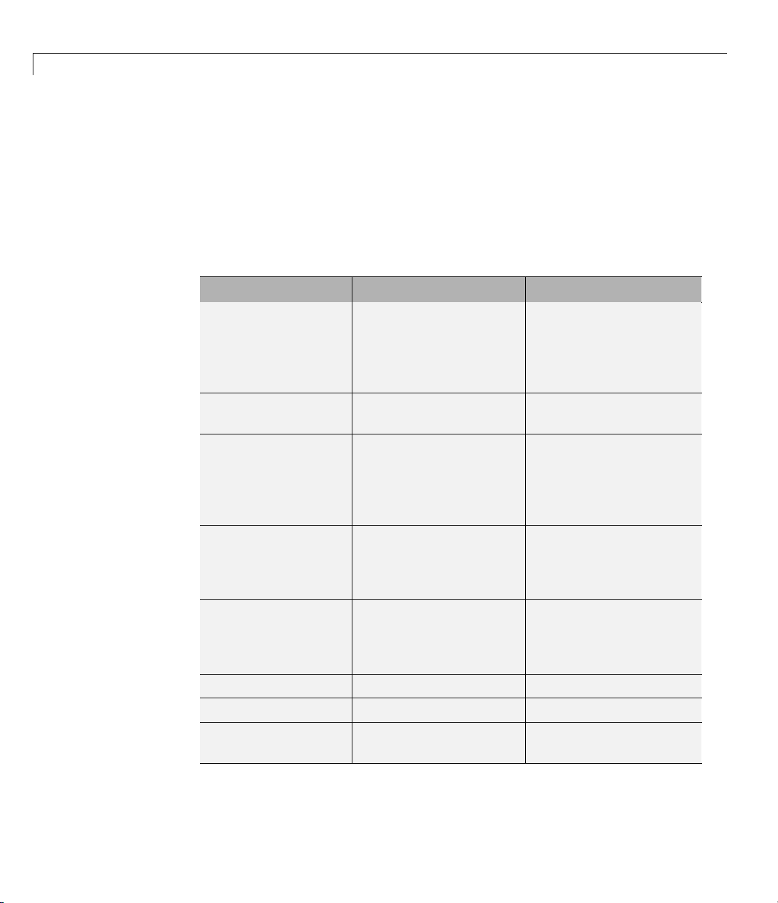
4 Create and load bodies for the animation object. The demo will use these

bodies to work with and display the simulated and actual flight trajectories. The first body is orange; it represents simul ate d data. The second body is blue; it represents the actual flight data.

2-28

idx1 = h.createBody('pa24-250_orange.ac','Ac3d'); idx2 = h.createBody('pa24-250_blue.ac','Ac3d');

Both bodies are AC3D format files. AC3D is one of several file formats that the a nimation objects support. FlightGear uses the same file format. The animation object reads in the bodies in the AC3D format and stores them as patches in the geometry object within the animation object.

Loading Recorded Data for Flight Trajectories

This series of commands loads the recorded flight trajectory data, which is contained in files in the

•

simdata – Contains simulated flight trajectory data, which is set up as a

6DoF array.

•

fltdata – Contains actual flight trajectory data, which is set up in a

custom format. To access this custom format data, the demo needs to

matlabroot\toolbox\aero\astdemos folder.

3-D Flight Data Playback

set the body object TimeSeriesSourceType parameter to Custom,then specify a custom read function.

1 Load the flight trajectory data.

load simdata load fltdata

2 Set the time series data for the two bodies.

h.Bodies{1}.TimeSeriesSource = simdata; h.Bodies{2}.TimeSeriesSource = fltdata;

3 Identify the time series for the second body as custom.

h.Bodies{2}.TimeSeriesSourceType = 'Custom';

4 Specify the custom read function to access the data in fltdata for

the second body. The demo provides the custom read function in

matlabroot\toolbox\aero\astdemos\CustomReadBodyTSData.m.

h.Bodies{2}.TimeseriesReadFcn = @CustomReadBodyTSData;

Displaying Body Geometries in a Figure Window

This command creates a figure object for the animation object.

h.show();

Playing Back Flight Trajectories Using the Animation Object

This command plays the animation bodies for the duration of the time series data. This illustrates the differences between the simulated and actual flight data.

h.play();

2-29

2 Using Aerospace Toolbox

2-30

Manipulating the Camera

This command series describes how you can manipulate the camera on the two bodies, and redisplay the animation. The object controls the camera position relative to the bodies in the animation. In the section “Playin g Back Flight Trajectories Usin g the Animation Object” on page 2-29, the camera obje ct uses a default value for the property. In this command series, the demo references a custom PositionFcn function, which uses a static position based on the position of the bodies; no dynamics are involved. The custom

matlabroot\toolbox\aero\astdemos folder.

1 Set the camera PositionFcn to the custom function

staticCameraPosition.

h.Camera.PositionFcn = @staticCameraPosition;

PositionFcn property of a camera

PositionFcn

PositionFcn function is located in the

3-D Flight Data Playback

2 Run the animation again.

h.play();

Manipulating Bodies

This sectio n illustrates some of the actions you can perform on bodie s.

Moving and Reposition ing Bodies. This series of commands illustrates how to move and reposition bodies.

1 Set the starting time to 0.

t=0;

2 Move the body to the starting position that is based on the time series data.

Use the Aero.Animation object

h.updateBodies(t);

Aero.Animation.updateBodies method.

3 Update the camera position using the custom PositionFcn

function set in the previous section. Use the Aero.Animation object

Aero.Animation.updateCamera method.

h.updateCamera(t);

4 Reposition the bodies by first getting the current body position, then

separating the bodies.

a Get the current body positions and rotations from the objects of both

bodies.

pos1 = h.Bodies{1}.Position; rot1 = h.Bodies{1}.Rotation; pos2 = h.Bodies{2}.Position; rot2 = h.Bodies{2}.Rotation;

b Separate and reposition the bodies by moving them to new positions.

h.moveBody(1,pos1 + [0 0 -3],rot1); h.moveBody(2,pos1 + [0 0 0],rot2);

2-31

2 Using Aerospace Toolbox

2-32

Creating a Transparency in the First Body. This series of commands illustrates how to create and attach a t ransparency to a body. The animation object stores the body geometry as patches. This example manipulates the transparency properties of these patches (see “Creating 3-D Models with Patches” in the MATLAB documentation).

Note The use of transparencies might decrease animation speed on platforms that use software OpenGL

rendering (see opengl in the MATLAB

documentation).

1 Change the body patch properties. Use the Aero.Body PatchHandles

property to get the patch handles for the first body.

patchHandles2 = h.Bodies{1}.PatchHandles;

2 Set the desired face and edge alpha values for the transparency.

3-D Flight Data Playback

desiredFaceTransparency = .3; desiredEdgeTransparency = 1;

3 Get the current face and edge alpha data and change all values to

the desired alpha values. In the figure, note the first body now has a transparency.

for k = 1:size(patchHandles2,1)

tempFaceAlpha = get(patchHandles2(k),'FaceVertexAlphaData');

tempEdgeAlpha = get(patchHandles2(k),'EdgeAlpha');

set(patchHandles2(k),...

'FaceVertexAlphaData',repmat(desiredFaceTransparency,size(tempFaceAlpha)));

set(patchHandles2(k),...

'EdgeAlpha',repmat(desiredEdgeTransparency,size(tempEdgeAlpha)));

end

2-33

2 Using Aerospace Toolbox

Changing the Color of the S econd Body. This series of commands

illustrates how to change the color of a body. The animation object stores the b ody geometry as patches. This example will manipulate the

FaceVertexColorData property of these patches.

1 Change the body patch properties. Use the Aero.Body PatchHandles

property to get the patch handles for the first body.

patchHandles3 = h.Bodies{2}.PatchHandles;

2 Set the patch color to red.

desiredColor = [1 0 0];

3 Get the current face color and data and propagate the new patch color,

red, to the face. Note the following:

• The

if condition prevents the windows from being colored.

name property is stored in the body geometry data

(h.Bodies{2}.Geometry.FaceVertexColorData(k).name).

• The code changes only the i ndices in

patchHandles3 with nonwindow

counterparts in the body geometry data.

Note If you cannot access the name property to determine the parts of the vehicle to color, you must use an alternative way to se lectively c olor your vehicle.

for k = 1:size(patchHandles3,1)

tempFaceColor = get(patchHandles3(k),'FaceVertexCData');

tempName = h.Bodies{2}.Geometry.FaceVertexColorData(k).name;

if isempty(strfind(tempName,'Windshield')) &&...

isempty(strfind(tempName,'front-windows')) &&...

isempty(strfind(tempName,'rear-windows'))

set(patchHandles3(k),...

'FaceVertexCData',repmat(desiredColor,[size(tempFaceColor,1),1]));

end

2-34

3-D Flight Data Playback

Turning Off the Landing Gear of the Second Body. This command series illustrates how to turn off the landing g ea r on the second body by turning off the visibility of all the vehicle parts associated with the landing gear.

Note The indices into the patchHandles3 vector are determined from the

name property. If you cannot access the name property to determine the

indices, you must use an alternative way to determine the indices that correspond to the geometry parts.

for k = [1:8,11:14,52:57]

set(patchHandles3(k),'Visible','off')

end

Using Aero.VirtualRealityAnimation Objects

The A eros pace Toolbox interface to virtual reality animation objects uses the Simulink 3D Animation software. See

Aero.Node,andAero.Viewpoint for details.

Aero.VirtualRealityAnimation,

1 Create and configure an animation object.

a Configure the animation object.

b Initialize that object.

2 Enable the tracking of changes to virtual worlds.

3 Load the animation world.

4 Load time series data for simulation.

5 Set coordination information for the object.

6 Add a chase helicopter to the object.

7 Load time series data for chase helicopter simulation.

8 Set coordination information for the new object.

9 Add a new viewpoint for the helicopter.

2-35

2 Using Aerospace Toolbox

10 Play the animation.

11 Create a new viewpoint.

12 Add a route.

13 Add another helicopter.

14 Remove bodies.

15 Revert to the original world.

Running the Demo

1 Start the MATLAB software.

2 Run the demo either by entering astvranim in the MATLAB Command

Window or by finding the demo entry (Visualize Aircraft Takeoff via the Simulink 3D Animation product) in the MATLAB Online Help and clicking

RunintheCommandWindowon its demo page.

2-36

While running, the demo performs several steps by issuing a series of commands, as explained below.

Creating and Configuring a Virtual Reality Animation Object

This series of commands creates an animation object and configures the object.

1 Create an animation object.

h = Aero.VirtualRealityAnimation;

2 Configure the animation object to set the number of frames per second

(

FramesPerSecond) property. This controls the rate at which frames are

displayed in the figure window.

h.FramesPerSecond = 10;

3 Configure the animation object to set the seconds of animation data per

second time scaling (

h.TimeScaling = 5;

TimeScaling) property.

3-D Flight Data Playback

The combination of FramesPerSecond and TimeScaling property determine the time step of the simulation. The settings in this demo result in a time step of approximately 0.5 s.

4 Specify the .wrl file for the vrworld object.

h.VRWorldFilename = [matlabroot,'/toolbox/aero/astdemos/asttkoff.wrl'];

The virtual reality animation object reads in the .wrl file.

Enabling Aero.Vir tualRealityAnimation Methods to Track Changes to Virtual Worlds

Aero.VirtualRealityAnimation methods that change the current virtual

reality world use a temporary these methods to work in a write-protected folder such as the following.

1 Copy the virtual world file, asttkoff.wrl,toatemporaryfolder.

.wrl file to manage those changes. To enable

astdemos,type

copyfile(h.VRWorldFilename,[tempdir,'asttkoff.wrl'],'f');

2 Set the asttkoff.wrl world filename to the copied .wrl file.

h.VRWorldFilename = [tempdir,'asttkoff.wrl'];

Loading the Animation World

Load the animation world described in the VRWorldFilename field of the animation object. When parsing the world, this method creates node objects for existing nodes with Simulink 3D Animation Viewer.

h.initialize();

DEF nam e s. The initialize method also opens the

2-37

2 Using Aerospace Toolbox

2-38

Displaying Figures

While working with this demo, you can capture a view of a scene with the

takeVRCapture tool. This tool is specific to the astvranim demo. To display

the initial scene, type

takeVRCapture(h.VRFigure);

3-D Flight Data Playback

A MATLAB figu r e window displays with the initial scene.

Loading Time Series Data for Simulation

Toprepareforsimulation,setthesimulationtimeseriesdata.

takeoffData.mat contains logged simulated data that you can use

to set the time series data. structure

1 Load the takeoffData.

2 Set the time series data for the node.

'StructureWithTime', which is a default data format.

load takeoffData

h.Nodes{7}.TimeseriesSource = takeoffData; h.Nodes{7}.TimeseriesSourceType = 'StructureWithTime';

takeoffData is set up as the Simulink

Aligning the Position and Rotation Data with Surrounding Virtual World Objects

The virtual reality animation object expects positions and rotations in aerospace body coordinates. If the input data coordinate system is different, as isthecaseinthisdemo,youmustcreateacoordinate transformation function to correctly line up the position and rotation data with the surrounding objects in the virtual world. This code should set the coordinate transformation function for the virtual reality animation. The custom transfer function for this demo is In this demo, if the input translation coordinates are transform function must adjust them as:

matlabroot/toolbox/aero/astdemos/vranimCustomTransform.m.

[x1,y1,z1],thecustom

[X,Y,Z] = -[y1,x1,z1]

To run this custom transformation function, type:

h.Nodes{7}.CoordTransformFcn = @vranimCustomTransform;

Viewing the Nodes in a Virtual Reality Animation Object

While working with this demo, you can view all the n odes currently in the virtual reality animation object with the

nodeInfo method.

2-39

2 Using Aerospace Toolbox

h.nodeInfo;

This method displays the nodes currently in your demo:

Node Information 1_v1 2 Lighthouse 3_v3 4 Terminal 5 Block 6_V2 7 Plane 8 Camera1

Adding a Chase Helicopter

As part of the demo, add a chase helicopter node to your demo. Use the

addNode method to add another node to the virtual reality animation object.

2-40

Note By default, each time you add or remove a node, or when you call the

saveas method, a message shows the current .wrl file location. To disable

this message, set the

'ShowSaveWarning' property in the virtual reality

animation object. You can disable this message before adding the chase helicopter.

1 Disable the message.

h.ShowSaveWarning = false;

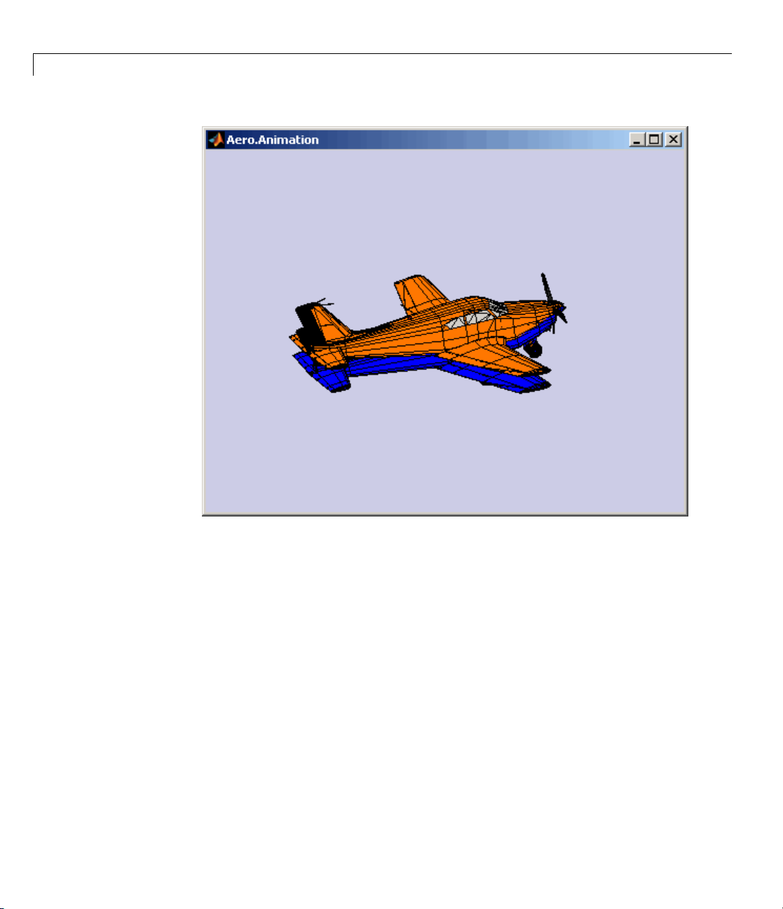
2 Add the chase helicopter node.

h.addNode('Lynx',[matlabroot,'/toolbox/aero/astdemos/chaseHelicopter.wrl']);

The helicopter appears in the Simulink 3D Animation Viewer.

3 Move the camera angle of the virtual reality figure to view the aircraft

and newly added helicopter.

set(h.VRFigure,'CameraDirection',[0.45 0 -1]);

4 View the scene with the chase helicopter.

takeVRCapture(h.VRFigure);

3-D Flight Data Playback

Loading Time Series Data for Simulation

Topreparetosimulatethechasehelicopter,setthesimulationtime series data.

chaseData.mat contains logged simulated data that you

2-41

2 Using Aerospace Toolbox

can use to set the time series data. chaseData is set up as the Simulink structure

1 Load the chaseData.

2 Set the time series data for the node.

'StructureWithTime', which is a default data format.

load chaseData

h.Nodes{2}.TimeseriesSource = chaseData;

Aligning the Chase Helicopter Position and Rotation Data with Surrounding Virtual World Objects

Use the custom transfer function to align the chase helicopter.

h.Nodes{2}.CoordTransformFcn = @vranimCustomTransform;

2-42

Adding a New Viewpoint

To add a viewpoint for the chase helicopter, use the addViewpoint method. New viewpoints appear in the Viewpoints menu of the Simulink 3D Animation Viewer. Type the following to add the viewpoint

Helicopter

h.addViewpoint(h.Nodes{2}.VRNode,'children','chaseView','View From Helicopter');

to the Viewpoints menu.

View From

3-D Flight Data Playback

Playing Back the Simulation

The play command animates the virtual reality world for the given position and angle for the duration of the time series data. Set the orientation of the viewpoint first.

1 Set the orientat ion of the viewpoint via the vrnode object associated with

the node object for the viewpoint.

setfield(h.Nodes{1}.VRNode,'orientation',[0 1 0 convang(160,'deg','rad')]);

set(h.VRFigure,'Viewpoint','View From Helicopter');

2 Play the animation.

h.play();

Adding a Route to the Camera1 Node

The vrworld has a Ride on the Plane viewpoint. To enable this viewpoint to function as intended, connect the plane position to the Camera1 node with the

addRoute method. This method add s a VRML ROUTE statement.

h.addRoute('Plane','translation','Camera1','translation');

2-43

2 Using Aerospace Toolbox

Adding Another Helicopter and Viewing All Bodies Simultaneously

You can add another helicopter to the scene and also change the viewpoint to one that views all three bodies in the scene at once.

1 Add a new node, Lynx1.

h.addNode('Lynx1',[matlabroot,'/toolbox/aero/astdemos/chaseHelicopter.wrl']);

2 Change the viewpoint to one that views all three bodies.

set(h.VRFigure,'Viewpoint','See Whole Trajectory');

2-44

3-D Flight Data Playback

Removing Bodies

Use the removeNode method to remove the second helicopter. To obtain the name of the node to remove, use the

1 View all the nodes.

h.nodeInfo

nodeInfo method.

2-45

2 Using Aerospace Toolbox

Node Information 1 Lynx1_Inline 2 Lynx1 3 chaseView 4 Lynx_Inline 5 Lynx 6_v1 7 Lighthouse 8_v3 9 Terminal 10 Block 11 _V2 12 Plane 13 Camera1

2 Remove the Lynx1 node.

h.removeNode('Lynx1');

2-46

3 Change the viewpoint to one that views the whole trajectory.

set(h.VRFigure,'Viewpoint','See Whole Trajectory');

4 Check that you have removed the node.

h.nodeInfo

Node Information 1 chaseView 2 Lynx_Inline 3 Lynx 4_v1 5 Lighthouse 6_v3 7 Terminal 8 Block 9_V2 10 Plane 11 Camera1

3-D Flight Data Playback

The following figure is a view of the entire trajectory with the third body removed.

Reverting to the Original World

Theoriginalfilenameisstoredinthe'VRWorldOldFilename' property of the virtual reality animation object. To display the original world, set

'VRWorldFilename' to the original name and reinitialize it.

2-47

2 Using Aerospace Toolbox

1 Revert to the original world, 'VRWorldFilename'.

h.VRWorldFilename = h.VRWorldOldFilename{1};

2 Reinitialize the restored world.

h.initialize();

Closing and Deleting Worlds

To close and delete a world, use the delete method.

h.delete();

Using Aero.FlightGearAnimation Objects

The Aerospace Toolbox interface to the FlightGear flight simulator enables you to visualize flight data in a three-dimensional environment. The third-party FlightGear simulator is an open source software package available through a GNU obtain and install the third-party FlightGear flight simulator. It then explains how to play back 3-D flight data by using a FlightGear demo, provided with your Aerospace Toolbox software, as an example.

General Public License (GPL). This section explains how to

2-48

• “About the FlightGear Interface” on page 2-48

• “Configuring Your Computer for FlightGear” on page 2-49

• “Installing and Starting FlightGear” on page 2-52

• “Working with the Flight Simulator Interface” on page 2-53

• “Running the Demo” on page 2-56

About the FlightGear Interface

The FlightGear flight simulator interface included with the Aerospace Toolbox product is a unidirectional transmission link from the MATLAB software to FlightGear using FlightGear’s published protocol. Data is transmitted via UDP network packets to a running instance of FlightGear. The toolbox supports multiple standard binary distributions of FlightGear. See “Working with the Flight Simulator Interface” on page 2-53 for interface details.

net_fdm binary data exchange

3-D Flight Data Playback

FlightGear is a separate software entity neither created, owned, nor maintained by The MathWorks.

• To report bugs in or request enhancements to the Aerospace Too lbox

FlightGear interface, contact MathWorks Technical Support at http://www.mathworks.com/contact_TS.html.

• To report bugs or request enhancements to FlightGear itself, visit

www.flightgear.org and use the contact page.

Obtaining FlightG ear. You can obtain FlightGear from

www.flightgear.org in the download area or by ordering CDs from

FlightGear. The download area contains extensive documentation for installation and configuration. Because FlightGear is an open source project, source downloads are also available for customization and porting to custom environments.

Configuring Your Computer for FlightGear

You must have a high performance graphics card with stable drivers to use FlightGear. For more information, see the FlightGear CD distribution or the hardware requirements and documentation areas of the FlightGear Web site,

www.flightgear.org.

The MathWorks tests of FlightGear’s performance and stability indicate significant sensitivity to computer video cards, driver versions, and driver settings. You need OpenGL support with hardware acceleration activated. The OpenGL settings are particularly important. Withoutpropersetup, performance can drop from about a 3 0 frames-per-second (fps) update rate to less than 1 f ps.

Graphics Recommendations for Microsoft Windows. The MathWorks recommends the following for Windows

users:

• Choose a graphics card with good OpenGL performance.

• Always use the latest tested and stable driver release for your video card.

Test the driver thoroughly on a few computers before deploying to others.

For Microsoft

Windows XP systems running on x86 (32-bit) or AMD-64/EM64T chip architectures, the graphics card operates in the unprotected kernel space known as Ring Zero. This means that glitches in

2-49

2 Using Aerospace Toolbox

the driver can cause the Windows operating system to lock or crash. Before buying a large number of computers for 3-D applications, test, with your vendor, one or two computers to find a combination of hardware, operating system, drivers, and settings that are stable for you r applications.

Setting Up OpenGL Graphics on Windows. For complete information on Silicon Graphics OpenGL settings, refer to the documentation at the OpenGL Web site,

Follow these steps to optimize your video card settings. Your driver’s panes might look different.

1 Ensure that you have activated the OpenGL hardware acceleration on

your video card. On Windows, access this configuration through Start > Settings > Control Panel > Display, which opens the following dialog box. Select the Settings tab.

www.opengl.org.

2-50

2 Click the Advanced button in the lower right of the dialog box, which

opens the graphics card’s custom configuration dialog box, and go to the

3-D Flight Data Playback

OpenGL tab. For an ATI Mobility Radeon 9000 video card, the OpenGL pane looks like this:

3 For best performance, move the Main Settings slider near the top of the

dialog box to the Performance end of the slider.

4 If stability is a problem, try other screen resolutions, other color depths in

the Displays pane, and other OpenGL acceleration modes.

Many cards perform m uch better at 16 bits-per-pixel color depth (also known as 65536 color mode, 16-bit color). For example, on an ATI Mobility Radeon 9000 running a given model, 30 fps are achieved in 16-bit color mode, while 2 fps are achieved in 32-bit color mode.

2-51

2 Using Aerospace Toolbox

Setup on Linux®,MacOS®X, and Other Platforms. FlightGear

distributions are available for Linux, Mac OS X, and other UNIX from the FlightGear Web site, platforms, like Windows, requires careful configuration of graphics cards and drivers. Consult the documentation and hardware requirements sections at the FlightG ear Web site.

Using MATLAB Graphics Controls to Configure Your OpenGL Settings.

You can also control your OpenGL rendering from the MATLAB command line with the MATLAB Graphics command reference for more information.

www.flightgear.org. Installationonthese

opengl command. Consult the opengl

platforms

Installing and Starting FlightGear

The extensive FlightGear documentation guides you through the installation in detail. Consult the documentation section of the FlightGear Web site for complete installation instructio n s:

Keep the following points in mind:

• Generous central processor speed, system and video R AM, and virtual

memory are essential for good flight simulator performance.

The MathWorks recommends a minimum of 512 megabytes of system RAM and 128 megabytes o f video RAM for reasonable performance.

www.flightgear.org.

2-52

• Be sure to have sufficient disk space for the FlightGear download a nd

installation.

• The MathWorks recommends configuring your computer’s graphics card

before you install FlightGear. See the preceding section, “Configuring Your Computer for FlightGear” on page 2-49.

• Shutting down all running applications (including the MATLAB software)

before installing FlightGear is recommended.

• The MathWorks tests indicate that the operational stability of FlightGear

is especially sensitive during startup. It is best to not move, resize, mouse over, overlap, or cover up the FlightGear window until the initial simulation scene appears after the startup splash screen fades out.

3-D Flight Data Playback

• The current releases of FlightGear are optimized for flight visualization at

altitudes below 100,000 feet. FlightGear does not work well or at all with very high altitude and orbital views.

The Aerospace Toolbox product supports FlightGear on a number of platforms (

http://www.mathworks.com/products/aerotb/requirements.html). The

following table lists the properties you should be aware of before you start to use FlightGear.

FlightGear Property

FlightGearBaseDirectory

GeometryModelName

Folder Description

FlightGear installation folder.

Platforms

Windows

Sun™ Solaris™ or

Typica l Lo cation

C:\Program Files\FlightGear

(default)

Directory into which you installed FlightGear

Linux

Mac

/Applications

(folder to which you d ragged the FlightGear icon)

Model geometry folder

Windows

C:\Program Files\FlightGear\data\Aircraft\HL20

(default)

Solaris or Linux

Mac

$FlightGearBaseDirectory/data/Aircraft/HL20

$FlightGearBaseDirectory/FlightGear.app/Contents/Resources/data/Aircraft/HL20

Working with the Flight Simulator Interface

The Aerospace Toolbo x product provides a demo named Displaying Flight Trajectory Data, which shows you how you can visualize flight trajectories withFlightGearAnimationobject. Thedemoisintendedtobemodified depending on the particulars of your FlightGear installation. This section explains how to run this demo. Use this demo as an example to play back your own 3-D flight d ata with FlightGear.

2-53

2 Using Aerospace Toolbox

YouneedtohaveFlightGearinstalledand configured before attempting to simulate this model. See “About the FlightGear Interface” on page 2-48.

To run the demo:

1 Import the aircraft geometry into FlightGear.

2 Run the demo. The demo performs the following steps:

a Loads recorded trajectory data

b Creates a time series object from trajectory data

c Creates a FlightGearAnimation object

3 Modify the animation object properties, if needed.

4 Create a run script for launching FlightGear flight simulator.

5 Start FlightGear flight simulator.

6 Play back the flight trajectory.

2-54

The following sections describe howtoperformthesestepsindetail.

Importing the Aircraft G e ometry into FlightGear. Before running the demo, copy the aircraft geometry model into FlightGear. From the following procedures, choose the one appro priate for your platform. This section assumes that you have read “Installing and Starting FlightGear” on page 2-52.

If your platform is Windows:

1 Go to your installed FlightGear folder. O pen the data folder, then the

Aircraft folder: FlightGear\data\Aircraft\.

2 You may already have an HL20 subfolder there, if you have previously run

the Aerospace Blockset NASA HL-20 with FlightGear Interface demo. In this case, you don’t have to do anything, because the geometry model is the same.

Otherwise, copy the

matlabroot\toolbox\aero\aerodemos\ folder to the FlightGear\data\Aircraft\ folder. This folder contains the

HL20 folder from the

3-D Flight Data Playback

preconfigured geometries for the HL-20 simulation and HL20-set.xml. The file

matlabroot\toolbox\aero\aerodemos\HL20\models\HL20.xml

defines the geometry.

If your platform is Solaris or Linux:

1 Go to your installed FlightGear folder. O pen the data folder, then the

Aircraft folder: $FlightGearBaseDirectory/data/Aircraft/.

2 You may already have an HL20 subfolder there, if you have previously run

the Aerospace Blockset NASA HL-20 with FlightGear Interface demo. In thiscase,youdonothavetodoanything,becausethegeometrymodel is the same.

Otherwise, copy the

matlabroot/toolbox/aero/aerodemos/ folder to the $FlightGearBaseDirectory/data/Aircraft/ folder. This folder contains

the preconfigured geometries for the HL-20 simulation and The file

matlabroot/toolbox/aero/aerodemos/HL20/models/HL20.xml

HL20 folder from the

HL20-set.xml.

defines the geometry.

If your platform is Mac:

1 Open a terminal.

2 List the contents of the Aircraft folder. For example, type

ls $FlightGearBaseDirectory/data/Aircraft/

3 You may already have an HL20 subfolder there, if you have previously run

the Aerospace Blockset NASA HL-20 with FlightGear Interface demo. In this case, you do not have to do anything, because the geometry model is the same. Continue to “Running the Demo” on page 2-27.

Otherwise, copy the

matlabroot/toolbox/aero/aerodemos/

HL20 folder from the

folder to the

$FlightGearBaseDirectory/FlightGear.app/Contents/Resources/data/Aircraft/

2-55

2 Using Aerospace Toolbox

folder. This folder contains the preconfigured geometries for the HL-20 simulation and

matlabroot/toolbox/aero/aerodemos/HL20/models/HL20.xml

HL20-set.xml.Thefile

defines the geometry.

Running the Demo

1 Start the MATLAB software.

2 Run the demo either by entering astfganim in the MATLAB Command

Window or by finding the demo entry (Displaying Flight Trajectory Data) intheMATLABOnlineHelpandclickingRunintheCommandWindow on its demo page.

While running, the demo performs several steps by issuing a series of commands, as explained below.

Loading Recorded Flight Trajectory Data. The flight trajectory data for this example is stored in a comma separated value formatted file. Using

dlmread, the data is read from the f ile starting at row 1 and column 0, which

skips the header information.

2-56

tdata = dlmread('asthl20log.csv',',',1,0);

Creating a Time Series Object from Trajectory Data. Thetimeseries object, dataalongwiththetimearrayin

ts, is created from the latitude, longitude, altitude, and Euler angle

tdata using the MATLAB timeseries

command. Latitude, longitude, and Euler angles are also converted from degrees to radians using the

ts = timeseries([convang(tdata(:,[3 2]),'deg','rad') ...

tdata(:,4) convang(tdata(:,5:7),'deg','rad')],tdata(:,1));

convang function.

Creating a FlightGearAnimation Object. This series of commands creates a FlightGearAnimation object:

1 Opening a FlightGearAnimation object.

h = fganimation;

2 Setting FlightG earAnimation object properties for the time series.

h.TimeseriesSourceType = 'Timeseries'; h.TimeseriesSource = ts;

3-D Flight Data Playback

3 Setting FlightGearAnimation object properties relating to Flight

These properties include the path to the installation folder, the ve number, the aircraft geometry model, and network information fo

Gear.

rsion

rthe

FlightGear flight simulator.

h.FlightGearBaseDirectory = 'C:\Program Files\FlightGear191'; h.FlightGearVersion = '1.9.1'; h.GeometryModelName = 'HL20'; h.DestinationIpAddress = '127.0.0.1'; h.DestinationPort = '5502';

4 Setting the initial conditions (location and orientation) for the FlightGear

flight simulator.

h.AirportId = 'KSFO'; h.RunwayId = '10L'; h.InitialAltitude = 7224; h.InitialHeading = 113; h.OffsetDistance = 4.72; h.OffsetAzimuth = 0;

5 Setting the seconds of animation data per second of wall-clock time.

h.TimeScaling = 5;

6 Checking the FlightGearAnimation object properties and their values.

get(h)

At this point, the demo stops running and returns the FlightGearAnimation object,

TimeseriesSource: [196x1 timeseries]

TimeseriesSourceType: 'Timeseries'

TimeseriesReadFcn: @TimeseriesRead

TimeScaling: 5

FramesPerSecond: 12

FlightGearVersion: '1.9.1'

OutputFileName: 'runfg.bat'

2-57

2 Using Aerospace Toolbox

FlightGearBaseDirectory: 'C:\Program Files\FlightGear191'

GeometryModelName: 'HL20'

DestinationIpAddress: '127.0.0.1'

DestinationPort: '5502'

AirportId: 'KSFO'

RunwayId: '10L'

InitialAltitude: 7224

InitialHeading: 113 OffsetDistance: 4.7200

OffsetAzimuth: 0

You can now set the object properties for data playback (see “Modifying the FlightGearAnimation Object Properties” on page 2-58).

Modifying the FlightGearAnimation Object Properties. Modify the FlightGearAnimation object properties as needed. If your FlightGear installation folder is other thanthatinthedemo(forexample, modify the

FlightGearBaseDirectory property by issuing the following

FlightGear),

command:

2-58

h.FlightGearBaseDirectory = 'C:\Program Files\FlightGear';

Similarly,ifyouwanttouseaparticularfilenamefortherunscript,modify the

OutputFileName property.

Verify the FlightGearAnimation object properties:

get(h)

You can now generate the run script (see “Generating the Run Script” on page 2-58).

Generating the Run Script. To start FlightGear with the desired initial conditions (location, date, time, weather, operating modes), it is best to create a run script by using the

GenerateRunScript(h)

GenerateRunScript command:

By default, GenerateRunScript saves the run script as a text file named

runfg.bat. You can specify a different name by modifying the

3-D Flight Data Playback

OutputFileName property of the FlightGearAnimation object, as described

in the previous step.

This file does not need to be generated each time the data is viewed, only when the desired initial conditions or FlightGear information changes.

You are now ready to start FlightGear (see “Starting the FlightGear Flight Simulator” on page 2-59).

Starting the FlightGear Flight Simula tor. To start FlightGear from the MATLAB command prompt, use the

system command to execute the run

script. Provide the name of the output file created by GenerateRunScript as the argument:

system('runfg.bat &');

FlightGear starts in a separate window.

Tip With the FlightGear window in focus, press the V key to alternate between the different aircraft views: cockpit view, helicopter view, chase view, and so on.

You are now ready to play back data (see “Playing Back the Flight Trajectory” on page 2-59).

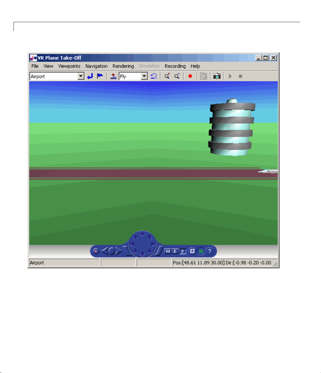
Playing Back the Flight Trajectory. Once FlightGear is running, the FlightGearAnimation object can start to communicate with FlightGear. To animate the flight trajectory data, use the play command:

play(h)

The following illustration shows a snapshot of flight data playback in tower view without yaw.

2-59

2 Using Aerospace Toolbox

2-60

Function Reference

Animation Objects (p. 3-3) Manipulate Aero.Animation objects

Body Objects (p. 3-4) Manipulate Aero.Body objects

Camera Objects (p. 3-5) Manipulate Aero.Camera objects

FlightGear Objects (p. 3-5)

Geometry O bjects (p. 3-6) Manipulate Aero.Geometry objects

Node Objects (p. 3-7) Manipulate Aero.Node objects

Viewpoint Objects (p. 3-8) Manipulate Aero.Viewpoint objects

Virtual Reality Objects (p. 3-9)

Axes Transfo rmations (p. 3-10) Transform axes of coordinate

Environment (p. 3-11) Simulate various aspects of aircraft

File Reading (p. 3-12) Read standard aerodynamic file

Flight Parameters (p. 3-12) Various flight parameters, including

Manipulate Aero.FlightGearAnimation objects

Manipulate Aero.VirtualRealityAnimation objects

systems to different types, such as Euler angles to quaternions and vice versa

environment, such as atmosphere conditions, gravity, magnetic fields, and wind

formats into the MATLAB interface

ideal airspeed correction, Mach number, and dynamic pressure

GasDynamics(p.3-12)

Various gas dynamics tables

3 Function Reference

Quaternion Math (p. 3-13) Common ma th ematical and

matrix operations, including quaternion multiplication, division, normalization, and rotating vector by quaternion

Time (p. 3-13)

Unit Conversion (p. 3-13) Convert common measurement units

Time calculations, including Julian dates, decimal year, and leap year

from one system to another, such as converting acceleration from feet per second to meters per second and vice versa

3-2

Animation Objects

addBody (Aero.Animation) Add loaded body to animation object

Aero.Animation Construct animation object

createBody (Aero.Animation) Create body and its associated

Animation Objects

and generate its patches

patches in animation

delete (Aero.Animation)

hide (Aero.Animation) Hide animation figure

initialize (Aero.Animation) Create animation object figure and

initIfNeeded (Aero.Animation) Initialize animation graphics if

moveBody (Aero.Animation)

play (Aero.Animation) Animate

removeBody (Aero.Animation) Remove one body from animation

show (Aero.Animation) Show animation object figure

updateBodies (Aero.Animation) Update bodies of animation object

updateCamera (Aero.Animation)

Destroy animation object

axes and build patches for bodies

needed

Move body in animation object

Aero.Animation object

given position/angle time series

Update camera in animation object

3-3

3 Function Reference

Body Objects

Body (Aero.Body) Construct body object for use with

animation object

findstartstoptimes (Aero.Body) Return start and stop times of time

series data

generatePatches ( Aero.Body) Generate patches for body with

loaded face , vertex, and color data

load (Aero.Body) Get geometry data from source

move (Aero.Body) Change animation body position and

orientation

update (Aero.Body) Change body position and orientation

as function of time

3-4

Camera Objects

Camera (Aero.Camera) Construct camera object for use with

Camera Objects

animation object

update (Aero.Camera)

FlightGear Objects

ClearTimer (Aero.Flig

delete (Ae

fganimat (Aero.Fl

Generat (Aero.F

initialize (Aero.FlightGearAnimation)

play ( A ero.FlightGearAnimation) Animate FlightGear flight simulator

SetTimer (Aero.FlightGearAnimation)

lightGearAnimation)

htGearAnimation)

ro.FlightGearAnimation)

ion

ightGearAnimation)

eRunScript

Update camera position based on time and position of other Aero.Body objects

Clear and de of Flig htGe

Destroy Fl

Construc object

Generat flight s

Set up F

using given position/angle time series

Set name of timer for animation of FlightGear flight simulator

lete timer for animation

ar flight simulator

ightGear animation object

t FlightGear animation

e run script for FlightGear

imulator

lightGear animation object

update (Aero.FlightGearAnimation) Update position data to FlightGear

animation object

3-5

3 Function Reference

Geometry Objects

Geometry (Aero.Geometry) Construct 3-D geometry for use with

animation object

read (Aero.Geometry)

Read geometry data using current reader

3-6

Node Objects

findstartstoptimes (A ero.Node) Return start and stop times for time

series data

move (Aero.Node) Changenodetranslationand

rotation

Node (Aero.Node) Create node object for use with

virtual reality animation

update (Aero.Node) Change node position and

orientation v ersus time data

3-7

3 Function Reference

Viewpoint Objects

Viewpoint (Aero.Viewpoint) Create viewpoint object for use in

virtual reality animation

3-8

Virtual Reality Objects

addNode (Aero.VirtualRealityAnimation)

addRoute (Aero.VirtualRealityAnimation)

addViewpoint (Aero.VirtualRealityAnimation)

delete (Aero.VirtualRealityAnimation)

initializ (Aero.Vir

nodeInfo (Aero.VirtualRealityAnimation)

play (Aero.VirtualRealityAnimation) Animate virtual reality world for

remove (Aero

remov (Aer

saveas (Aero.VirtualRealityAnimation)

tualRealityAnimation)

Node

.VirtualRealityAnimation)

eViewpoint

o.VirtualRealityAnimation)

Add existing node to current virtual reality world

Add VRML ROUTE statement to virtual reality animation

Add viewpoint for virtual reality animation

Destroy virtual reality animation object

Create and populate virtual reality animation object

Create list of nodes associated with virtual reality animation object

given position and angle in time series data

Remove node from virtual reality animation object

Remove viewpoint node from virtual reality animation

Save vi rtu al reality world associated with virtual reality animation object

ateNodes

upd

ro.VirtualRealityAnimation)

(Ae

VirtualRealityAnimation (Aero.VirtualRealityAnimation)

Change virtual reality animation node position and orientation as function of time

Construct virtual reality animation object

3-9

3 Function Reference

Axes Transformations

angle2dcm

angle2quat

dcm2alphabeta

dcm2angle

dcm2latlon

dcm2quat

dcmbody2wind

dcmecef2ned Convert geodetic latitude and

ecef2lla Convert Earth-centered Earth-fixed

geoc2geod

Create direction cosine matrix from rotation angles

Convert rotation angles to quaternion

Convert direction cosine matrix to angle of attack and sideslip angle

Create rotation angles from direction cosine matrix

Convert direction cosine matrix to geodetic latitude and longitude

Convert direction cosine matrix to quaternion

Convert angle of attack and sideslip angletodirectioncosinematrix

longitude to direction cosine matrix

(ECEF) coordinates to geo detic coordinates

Convert geocentric latitude to geodetic latitude

3-10

geod2geoc

lla2ecef Convert geodetic coordinates to

quat2angle

quat2dcm

Convert g eodetic latitude to geocentric latitude

Earth-centered Earth-fixed (ECEF) coordinates

Convert quaternion to rotation angles

Convert quaternion to direction cosine matrix

Environment

atmoscira

atmoscoesa

atmosisa

atmoslapse

atmosnonstd

atmosnrlmsise00 Implement mathematical

atmospa

geoide

gravitycentrifugal Implement centrifugal effect of

grav

gm96

itysphericalharmonic

Use COSPAR International Reference Atmos phere 1986 model

Use 1976 COESA model

Use International Standard Atmosphere model

Use Lapse Rate Atmosphere model

Use climatic data from MIL-STD-210 or MIL-HDBK-310

representation of 2001 United States Naval Research Laboratory Mass Spectrometer and Incoherent Scatter Radar Exosphere

Calculate pressure altitude based on ambient pressure

Calculate geoid height as determined from EGM96 Geopotential Model

planetary gravity

ement spherical harmonic

Impl

resentation of planetary gravity

rep

gravitywgs84

gravityzonal Implement zonal harmonic

wrldmagm Use World Magne t ic Model

lement 1984 World Geodetic

Imp

tem (WGS84) representation of

Sys

rth’s gravity

representation of planetary gravity

3-11

3 Function Reference

File Reading

datcomimport

Flight Parame

airspeed

alphabeta Incidence a

dpressure

geocradius

machnumber

rrdelta

rrsigma

rrtheta

ters

Bring DATCOM file into MATLAB environment

Airspeed from velocity

nd sideslip angles

Compute dyn velocity a

Estimate r at geocent

Compute M

y and speed of sound

velocit

Compute

Comput

Compu

amic pressure using

nd density

adius of ellipsoid p lanet

ric latitude

ach number using

relative pressure ratio

erelativedensityratio

te relative temperature ratio

Gas Dynamics

3-12

flowfanno Fanno line f low relations

flowisentropic Isentropic flow ratios

flownormalshock

flowprandtlmeyer Calculate Prandtl-Meyer functions

flowrayleigh Rayleigh line flow relations

Normal shock relations

for expansion waves

Quaternion Math

Time

quatconj

quatdivide Divide quaternion by another

quatinv

quatmod

quatmultip

quatnorm

quatnorma

quatrota

decyea

ndate

julia

year

leap

mjuliandate

lize

Calculate conjugate of quaternion

quaternion

Calculate inverse of quaternion

Calculate modulus of quaternion

Calculate product of two quaternions

Calculate norm of quaternion

Normalize

Rotate vector by quaternion

Calculate decimal year

Calculate Julian date

Dete

ulate modified Julian date

Calc

quaternion

rmine leap year

Unit Conversion

convacc

convang

convangacc

Convert from acceleration units to desired acceleration units

Convert from angle units to desired angle units

Convert from angular acceleration units to desired angular acceleration units

3-13

3 Function Reference

convangvel

convdensity

convforce Convert from force units to desired

convlength

convmass

convpres

convtemp

Convert from angular velocity units to desired angular velocity units

Convert from density units to desired density units

force units

Convert from length units to desired length units

Convert from mass units to desired mass units

Convert from pressure units to desired pressure units

Convert from temperature units to desired temperature units

3-14

Alphabetical List

Aero.Animation.addBody

Purpose Add loaded body to animation object and generate its patches

Syntax idx = addBody(h,b)

idx = h.addBody(b)

Description idx = addBody(h,b) and idx = h.addBody(b) add a loaded body, b,

to the animation object thebodytobeadded.

h and generates its patches. idx is the index of

Input Arguments

Output

idx

Animation object.

Loaded body.

Index of the body to be added.

Arguments

Examples Add a second body to the list that is a pointer to the first body. This

means that if you change the properties of one body, the properties of the other body change correspondingly.

h = Aero.Animation; idx1 = h.createBody('pa24-250_orange.ac','Ac3d'); b = h.Bodies{1}; idx2 = h.addBody(b);

4-2

addNode (Aero.VirtualRealityAnimation)

Purpose Add existing node to current virtual reality world

Syntax addNode(h, node_name, wrl_file)

h.addNode(node_name, wrl_file)

Description addNode(h, node_name, wrl_file) and h.addNode(node_name,

wrl_file)

reality world. The taken. points to) the names in the same added. You must specify the full path for this file. The vrnode object associated with the node object must be defined using a in the Transform.

add an existing node, node_name, to the current virtual

wrl_file isthefilefromwhichthenewnodeis

addNode adds a new node named node_name, which contains (or

wrl_file. node_name must be unique from other node

.wrl file. wrl_file must contain the node to be

DEF statement

.wrl file. This method creates a node object on the world of type

When you use the

.wrl file will be added to the virtual reality animation object under one

addNode method to add a node, all the objects in the

node. If you want to add separate nodes for the objects in the placeeachnodeinaseparate

.wrl file.

Example AddnodetoworlddefinedinchaseHelicopter.wrl.

h = Aero.VirtualRealityAnimation;

h.VRWorldFilename = [matlabroot,'/toolbox/aero/astdemos/asttkoff.wrl'];

copyfile(h.VRWorldFilename,[tempdir,'asttkoff.wrl'],'f');

h.VRWorldFilename = [tempdir,'asttkoff.wrl'];

h.initialize();

h.addNode('Lynx',[matlabroot,'/toolbox/aero/astdemos/chaseHelicopter.wrl']);

See Also Aero.Node, move, removeNode, updateNodes,

Aero.VirtualRealityAnimation

.wrl file,

4-3

addRoute (Aero.VirtualRealityAnimation)

Purpose Add VRML ROUTE statement to virtual reality animation

Syntax addRoute(h, nodeOut, eventOut, nodeIn, eventIn)

h.addNode(nodeOut, eventOut, nodeIn, eventIn)

Description addRoute(h, nodeOut, eventOut, nodeIn, eventIn) and

h.addNode(nodeOut, eventOut, nodeIn, eventIn) add a VRML

ROUTE statement to the virtual reality animation, where is the node from which information is routed, eventOut is the event (property),

eventIn is the receiving event (property).

Examples Add a ROUTE command to connect the Plane position to the Camera1

node.

h = Aero.VirtualRealityAnimation;

h.VRWorldFilename = [matlabroot,'/toolbox/aero/astdemos/asttkoff.wrl'];

copyfile(h.VRWorldFilename,[tempdir,'asttkoff.wrl'],'f');

h.VRWorldFilename = [tempdir,'asttkoff.wrl'];

h.initialize();

h.addNode('Lynx',[matlabroot,'/toolbox/aero/astdemos/chaseHelicopter.wrl']);

h.addRoute('Plane','translation','Camera1','translation');

nodeIn isthenodetowhichinformationisrouted,and

nodeOut

Mathworks AEROSPACE TOOLBOX 2 user guide

Specifications and Main Features

Frequently Asked Questions

User Manual

Getting Started

Product Overview

Related Products

Getting Online Help

Exploring the Toolbox

Using the MATLAB Help System for Documentation and Demos

Using Aerospace Toolbox

Defining Coordinate Systems

Fundamental Coordinate System Concepts

Definitions

Approximations

Motion with Respect to Other Planets

Coordinate Systems for Modeling

Body Coordinates

Wind Coordinates

Coordinate Systems for Navigation

Geocentric and Geodetic Latitudes

NED Coordinates

ECI Coordinates

ECEF Coordinates

Coordinate Systems for Display

References

Defining Aerospace Units

Importing Digital DATCOM Data

Overview

Example of a USAF Digital DATCOM File

Importing Data from DATCOM Files

Examining Imported DATCOM Data

Filling in Missing DATCOM Data

Plotting Aerodynamic Coefficients

Plotting Lift Curve Moments

Plotting Drag Polar Moments

Plotting Pitching Moments

3-D Flight Data Playback

Aerospace Toolbox Animation Objects

Using Aero.Animation Objects

Running the Demo

Creating and Configuring an Animation Object

Loading Recorded Data for Flight Trajectories

Displaying Body Geometries in a Figure Window

Playing Back Flight Trajectories Using the Animation Object

Manipulating the Camera

Manipulating Bodies

Using Aero.VirtualRealityAnimation Objects

Running the Demo

Creating and Configuring a Virtual Reality Animation Object

Loading the Animation World

Displaying Figures

Loading Time Series Data for Simulation

Viewing the Nodes in a Virtual Reality Animation Object

Adding a Chase Helicopter

Loading Time Series Data for Simulation

Adding a New Viewpoint

Playing Back the Simulation

Adding a Route to the Camera1 Node

Adding Another Helicopter and Viewing All Bodies Simultaneously

Removing Bodies

Reverting to the Original World

Closing and Deleting Worlds

Using Aero.FlightGearAnimation Objects

About the FlightGear Interface

Configuring Your Computer for FlightGear

Installing and Starting FlightGear

Working with the Flight Simulator Interface

Running the Demo

Function Reference

Animation Objects

Body Objects

Camera Objects

FlightGear Objects

Geometry Objects

Node Objects

Viewpoint Objects

Virtual Reality Objects

Axes Transformations

Environment