Mathworks AEROSPACE BLOCKSET 3 user guide

Download

Aerospace Blockse

User’s Guide

t™ 3

How to Contact The MathWorks

www.mathworks. comp.soft-sys.matlab Newsgroup www.mathworks.com/contact_TS.html T echnical Support

suggest@mathworks.com Product enhancement suggestions

bugs@mathwo doc@mathworks.com Documentation error reports service@mathworks.com Order status, license renewals, passcodes

info@mathwo

com

rks.com

Web

Bug reports

Sales, prici

ng, and general information

508-647-7000 (Phone)

508-647-7001 (Fax)

The MathWorks, Inc. 3 Apple Hill Drive Natick, MA 01760-2098

For contact information about worldwide offices, see the MathWorks Web site.

Aerospace Blockset™ User’s Guide

The software described in this document is furnished under a license agreement. The software may be used or copied only under the terms of the license agreement. No part of this manual may be photocopied or reproduced in any form without prior written consent from The MathW orks, Inc.

FEDERAL ACQUISITION: This provision applies to all acquisitions of the Program and Documentation by, for, or through the federal government of the United States. By accepting delivery of the Program or Documentation, the government hereby agrees that this software or documentation qualifies as commercial computer software or commercial computer software documentation as such terms are used or defined in FAR 12.212, DFARS Part 227.72, and DFARS 252.227-7014. Accordingly, the terms and conditions of this Agreement and only those rights specified in this Agreement, shall pertain to and govern theuse,modification,reproduction,release,performance,display,anddisclosureoftheProgramand Documentation by the federal government (or other entity acquiring for or through the federal government) and shall supersede any conflicting contractual terms or conditions. If this License fails to meet the government’s needs or is inconsistent in any respect with federal procurement law, the government agrees to return the Program and Docu mentation, unused, to The MathWorks, Inc.

Trademarks

MATLAB and Simulink are registered trademarks of The MathWorks, Inc. See

www.mathworks.com/trademarks for a list of additional trademarks. Other product or brand

names may be trademarks or registered trademarks of their respective holders.

Patents

The MathWorks products are protected by one or more U.S. patents. Please see

www.mathworks.com/patents for more information.

Revision History

July 2002 Online only New for V ersion 1.0 (Release 13) July 2003 Online only Revised for Version 1.5 (Release 13SP1) June 2004 Online only Revised for Version 1.6 (Release 14) October 2004 Online only Revised for Version 1.6.1 (Release 14SP1) March 2005 Online only Revised for Version 1.6.2 (Release 14SP2) May 2005 Online only Revised for Version 2.0 (Release 14SP2+) September 2005 First printing Revised for Version 2.0.1 (Release 14SP3) March 2006 Online only Revised for Version 2.1 (Release 2006a) September 2006 Online only Revised for Version 2.2 (Release 2006b) March 2007 Online only Revised for Version 2.3 (Release 2007a) September 2007 Second printing Revised for Version 3.0 (Release 2007b) March 2008 Online only Revised for Version 3.1 (Release 2008a) October 2008 Online only Revised for Version 3.2 (Release 2008b) March 2009 Online only Revised for Version 3.3 (Release 2009a) September 2009 Online only Revised for Version 3.4 (Release 2009b) March 2010 Online only Revised for Version 3.5 (Release 2010a)

Getting Started

Product Overview ................................. 1-2

Real-Time Workshop Code Generation Support Embedded MATLAB Function Support

................ 1-2

......... 1-2

Contents

Getting Started

• “Product Overview” on page 1-2

• “Related Products” on page 1-4

• “Running a Demo Model” on page 1-5

• “Learning More” on page 1-17

1 Getting Started

Product Overview

The Aerospace Blockset™ product lets you model aerospace systems in the Simulink

and MATLAB®environments. The Aerospace Blockset product brings the full power of Simulink to aerospace system design, integration, and simulation by providing key aerospace subsystems and components in the adaptable Simulink block format. From environmental models to equations of motion, from gain scheduling to animation, the blockset gives you the core components to assemble a broad range of large aerospace system architectures rapidly and efficiently.

YoucanusetheAerospaceBlocksetand Simulink products to develop your aerospace system concepts and to efficiently revise and test your models throughout the life cycle of your design. Animate your aerospace motion simulations with MATLAB Graphics or the optional Simulink

Animation™ viewer.

Real-Time Workshop Code Generation Support

UsetheAerospaceBlocksetsoftwarewiththeReal-TimeWorkshop®software to automatically generate code for real-time execution in rapid prototyping and for hardware-in-the-loop systems.

Embedded MATLAB Function Support

The Aerospace Blockset product supports the following Aerospace Toolbox quaternion functions in the Embedded MATLAB Function block:

1-2

onj

quatc quatinv quatmod

multiply

quat quatdivide quatnorm

normalize

quat

further information on using the Embedded MATLAB Function block, see:

For

ing the Embedded MATLAB

• “Us

Function Block” in Simulink User’s Guide

Product Overview

• asbQuatEML demo, which demonstrates quaternions and models the

equations

1-3

1 Getting Started

Related Products

In this section...

“Requirements for the Aerospace Blockset Product” on page 1-4

“Other Related Products” on page 1-4

Requirements for the Aerospace Blockset Product

In particular, the Aerospace Blockset product requires current versions of these products:

• MATLAB

• Aerospace Toolbox

• Simulink

Other Related Products

The related products listed on the Aerospace Blockset product page at theMathWorksWebsiteincludetoolboxesandblocksetsthatextendthe capabilities of the MATLAB and Simulink products. These products will enhance you r use of the Aerospace Blockset product in various applications.

1-4

For More Information About MathWorks Products

For more information about any MathWorks™ software products, see either

• The online documentation for that product if it is installed

• The MathWorks Web site at

www.mathworks.com; see the “Products” section

Running a Demo Model

In this section...

“Introduction” on page 1-5

“What This Demo Illustrates” on page 1-5

“Opening the M odel” on page 1-6

“Key Subsystems” on page 1-7

“Running the Demo” on page 1-10

“Modifying the Model” on page 1-12

Introduction

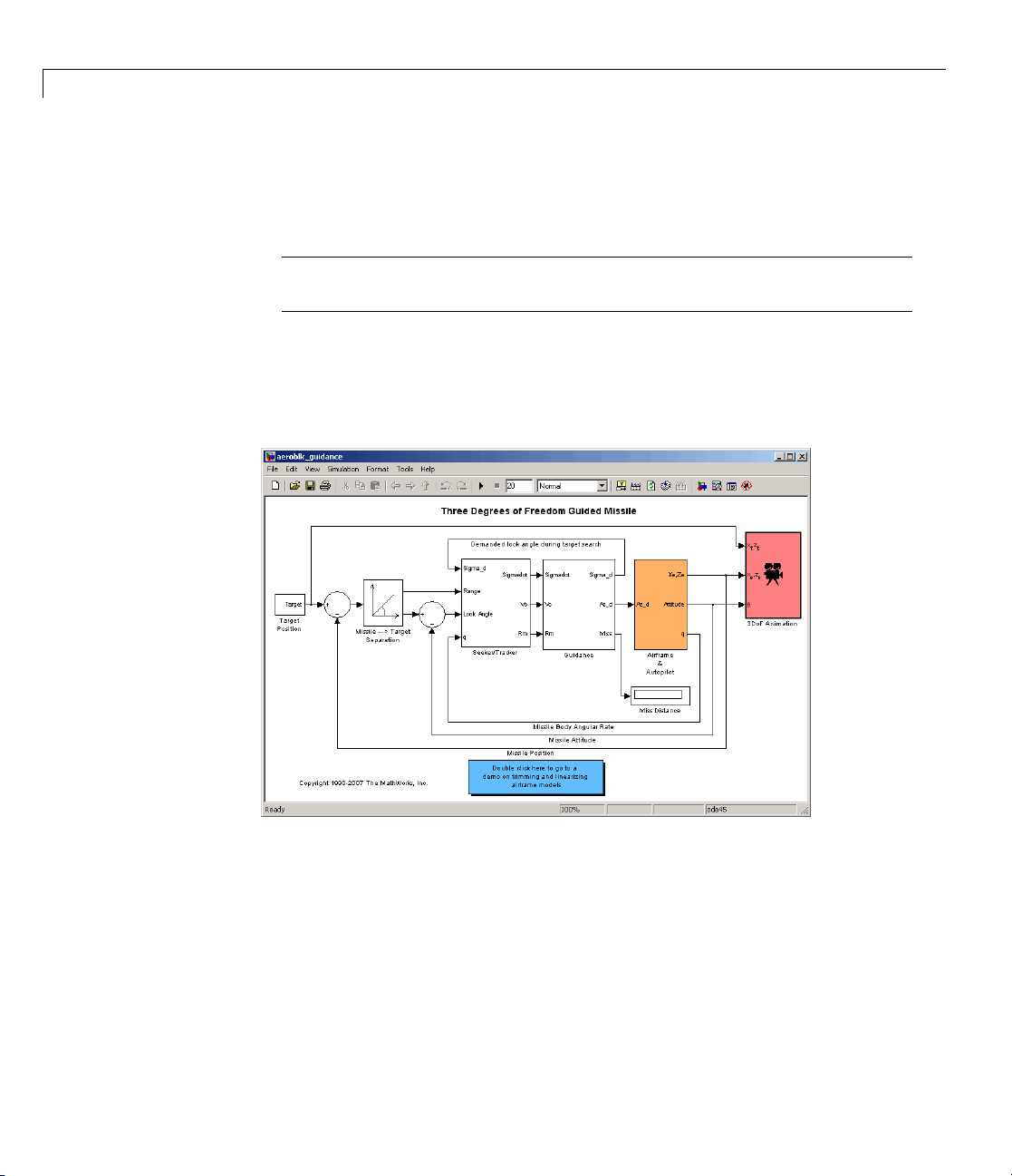
This section introduces a missile guidance model that uses blocks from the Aerospace B lockset software to simulate a three- degree-of-freedom missile guidance system, in conjunction with other Simulink blocks.

Running a Demo Model

The m o del simulates a missile guidance system with a target acquisition and interception subsystem. The model implements a nonlinear representation of the rigid body dynamics of the missile airframe, including aerodynamic forces and moments. The missile autopilot is based on the trimmed and linearized missile airframe. The missile homing guidance system regulates missile acceleration and measures the distance between the missile and its target.

For more information on this model, see Chapter 3, “Case Studies”.

What This Demo Illustrates

The missile guidance demo illustrates the following features of the blockset:

• Representing bodies and degrees of freedom with the Equations of Motion

library blocks

• Using the Aerospace Blockset blocks with other Simulink blocks

• Using the Aerospace Blockset blocks in the Stateflow

• Feeding in and feeding out Simulink signals to and from Aerospace

Blockset blocks with Actuator and Sensor blocks

charts

1-5

1 Getting Started

• Encapsulating groups of blocks into subsystems

• Visualizing and animating an aircraft with the Animation library blocks

Note The Stateflow module in this demo is precompiled and does not

require Stateflow software to be installed.

Opening the Model

To open the missile guidance demo, type the demo name, aeroblk_guidance, at the MATLAB command line. The model opens.

1-6

A Stateflow chart for the guidance control processor also appears.

Running a Demo Model

Alternatively, you can open demos through the MATLAB Help browser. To do this, click the Help button on the MATLAB Command Window. The MATLAB Help browser displays. In this browser, you can select Aerospace

Blockset>Demos>VehicleSystemModeling>Air>ThreeDegreeof Freedom Guided Missile.

Key Subsystems

The model impleme nts the missile environment, airframe, autopilot, and homing guidance system in subsystems.

• The Airframe & Autopilot subsystem implements the ISA Atmosphere

Model block, the Incidence & Airspeed block, and the 3DoF (Body Axes) block, along with other Simulink blocks.

The airframe model is a nonlinear representation of rigid body dynamics. The aerodynamic forces and moments acting on the missile body are generated from coefficients that are nonlinear functions of both incidence and Mach number.

1-7

1 Getting Started

1-8

• The model implements the missile autopilot as a classical three-loop design

using m easurements from an accelerometer located ahead of the missile’s center of gravity and from a rate g yro to provide additional damping.

Running a Demo Model

• The model implements the homing guidance system as two subsystems:

the G uidance subsystem and the Seeker/Tracker subsystem.

- The G uidance subsystem uses a Stateflow chart to control the tracker

directly by sending demands to the seeker gimbals.

- The Seeker/Tracker subsystem consists of Simulink blocks that control

the seeker gimbals to keep the seeker dish aligned with the target and provide the guidance law with an estimate of the sight line rate.

1-9

1 Getting Started

Running the Demo

Running a demo le run the demo, you visualization

ts you observe the model simulation in real time. After you can examine the resulting data in plots, graphs, and other

tools. To run the missile guidance model, follow these steps:

1 If it is not alr

2 From the Simulation menu, select Start. On Microsoft

eady open, open the

aeroblk_guidance demo.

Windows

systems, yo u can also click the start button in the model window toolbar.

The simulation proceeds until the m issile intercepts the target, which takes approximately 3 seconds. Once the interception has occurred, four scope figures open to display the following d ata:

a A three-dimensional animation of th e missile and target interception

course

1-10

b Plots that measure flight parameters over time, including Mach number,

fin demand, acceleration, and degree of incidence

Running a Demo Model

c A plot that measures gimbal versus true look angles

1-11

1 Getting Started

d A plot that measures missile and target trajectories

1-12

Modif

You c on si firs chan

ying the Model

an adjust the missile guidance model settings and examine the effects

mulation performance. Here are two modifications that you can try. The

t m od if ica tion adjusts the missile engine thrust. The second modification

ges the camera point of view for the interception animation.

Running a Demo Model

Adjusting the Thrust

As in any Simulink model, you can adjust aerospace model parameters from the MATLA B workspace. To demonstrate this, change the the m odel workspace and evaluate the results in the simulation.

1 Open the aeroblk_guidance model.

2 In the MATLAB desktop, find the Thrust variable in the Workspace pane.

Thrust variable in

The Thrust variable is defined in the aeroblk_guid_dat.m file, which the

aeroblk_guidance model uses to populate parameter and variable v alu es.

By default, the

3 Single-click the Thrust variable to select it. To edit the value, right-click

the

Thrust variable and select Edit Value. Change the value to 4500.

Thrust variableshouldbesetto10000.

Beforeyourunthedemoagain,locate the Miss Distance (Display) block display in the

aeroblk_guidance model.

1-13

1 Getting Started

Miss Distance Display

1-14

Start the demo, and after it finishes, note the miss distance display again. The miss distance should become greater than the original distance. You can experiment w ith different values in the

Thrust variable and assess the

effects on missile accuracy.

Changing the Animation Point of View

By default, the missile animation view is Fly Alongside, which means the view tracks with the missile’s flight path. You can easily change the animation point of view by adjusting a parameter of the 3DoF Animation block:

1 Open the aeroblk_guidance model, and double-click the 3DoF Animation

block. The Block Parameters dialog box appears.

Running a Demo Model

2 Change the view to Cockpit.

3 Click the OK button.

Run the demo again, and watch the animation. Instead of moving alongside the missile’s flight path, the animation point of view lies in the cockpit. Upon target interception, the screen fills with blue, the target’s color.

1-15

1 Getting Started

1-16

You can experiment with different views to watch the animation from different perspectives.

Learning More

In this section...

“Using the MATLAB Help System for Documentation and Demos” on page 1-17

“Finding Aerospace Blo ck set Help” on p a ge 1-17

Using the MATLAB Help System for Documentation and Demos

TheMATLABHelpbrowserallowsyoutoaccessthedocumentationanddemo models for all the MathW orks products that you have installed. The online help includes an online search system.

Consult the Help for Using MATLAB section of the MATLAB Desktop Tools and Development Environment documentation for more about the MATLA B help system.

Learning More

Opening Aerospace Demos

To open an Aerospace Blockset demo from the Help browser, open the MATLAB Command Window and select Aerospace Blockset > Demos.

You can also open the Aerospace Blockset demos from the Start button of the MATLAB desktop:

1 Click the Start button.

2 Select Blocksets,thenAerospace,andthenDemos.

opens the Help browser with Demos selected in the Help Navigator

This

pane

ernatively, you can open the Demos window by entering

Alt

LAB command line.

MAT

nding Aerospace Blockset Help

is user’s guide also includes a reference chapter.

demos at the

1-17

1 Getting Started

• Appendix A, “Aerospace Units” explains the unit systems used by the

blockset.

1-18

Using the Aerospace Blockset Software

• “Introducing the Aerospace Blockset Libraries” on page 2-2

• “Creating Aerospace Models” on page 2-8

• “Building a Simple Actuator System” on page 2-10

• “About Aerospace Coordinate Systems” on page 2-16

• “Introducing the Flight Simulator Interface” on page 2-26

• “Working with the Flight Simulator Interface” on page 2-32

2 Using the Aerospace Blockset™ Software

Introducing the Aerospace Blockset Libraries

In this section...

“Introduction” on page 2-2

“Opening the Aerospace Blockset Library” on page 2-2

“Summary of Aerospace Blockset Libraries” on page 2-4

Introduction

Constructing a simple Aerospace Blockset model is easy to learn if you know how to create Simulink models. If you are not familiar with the Simulink product, please see the Simulink documentation. The Aerospace Blockset library is organized into hierarchical libraries of closely related blocks for use in the Simulink library.

Opening the Aerospace Blockset Library

You can open the Aerospace Blockset library from the Simulink Library Browser. The procedure is the same on Window s and UNIX

platforms.

2-2

Opening the Simulink Library Browser

To start the Simulink Library Browser, click the buttonintheMATLAB toolbar, or enter

simulink

at the command line.

Simulink Libraries

The libraries in the Simulink library Browser contain all the basic elements you need to construct a model. Look here for basic math operations, switches, connectors, simulation control elements, and other items that do not have a specific aerospace orientation.

Introducing the Aerospace Blockset™ Libraries

Opening the Aerospace Blockset Library

The Simulink Library Browser opens when you type simulink in the MATLAB

Command Window or click the

button. The left pane contains a list of

all the blocksets that you currently have installed.

The fir expand left of block

st item in the list is the Simulink library itself, which is already

ed to show the available Simulink libraries. Click the

any blockset name to expand the hierarchical list and display that

set’s libraries within the browser.

symbol to the

n the Aerospace Blockset window from the MATLAB command line,

To ope

ente

aerolib

ble-click any library in the window to display its contents. The following

Dou

ure shows the Aerospace Blockset library window.

fig

2-3

2 Using the Aerospace Blockset™ Software

For a complete list of all the blocks in the Aerospace Blockset library, see “Summary of Aerospace Blockset Libraries” on page 2-4.

See the Simulink documentation for a complete description of the Simulink Library Browser.

2-4

SummaryofAerospaceBlocksetLibraries

The blocks of the A erospace Blockset library are organized into these libraries.

Actuators Library

The Actuators library provides blocks for representing linear and nonlinear actuators with saturation and rate limits.

Aerodynamics Library

The Aerodynamics library provides the Aerodynamic Forces and Moments block using the aerodynamic coefficients,dynamicpressure,centerofgravity, and center of pressure.

Animation Library

The Animation library provides the animation blocks for visualizing flight paths and trajectories and for working with a flight simulator interface. The

Introducing the Aerospace Blockset™ Libraries

Animation library contains the MATLAB-Based Animation, Flight Simulator Interfaces, and Anima tion Support Utilities sublibraries.

MATLAB-Based Animation Sublibrary. The MATLAB-Based Animation sublibrary provides the 3DoF Animation block and the 6DoF Animation block. Using the animation blocks, you can visualize flight paths and trajectories.

Flight Simulator Interfaces Sub li br ary. The Flight Simulator In terfa c es sublibrary provides the interface blocks to connect the Aerospace Blockset product to the third-party FlightGear flight simulator.

Animation Support Utilities Sublibrary. The Animation Support Utilities sublibrary provides additional blocks for running the FlightGear flight simulator. It contains a joystick interface for Windows platform and a block that lets you set the simulation pace.

Environment L ibrary

The E nvironment library provides blocks that simulate aspects of an aircraft and spacecraft environment, such as atmospheric conditions, gravity, magnetic fields, and wi nd. The Environment library contains the Atmosphere, Gravity, and Wind sublibraries.

Atmosphere Sublibrary. The Atmosphere sublibrary provides general atmospheric models, such as ISA and COESA, and other blocks, including nonstandard day simulations, lapse rate atmosphere, and pressure altitude.

Gravity Sublibrary. The Gravity sublibrary provides blocks that calculate the g ravity and magnetic fields for any point on the Earth.

Wind Sublibrary. The Wind sublibrary provides blocks for wind-related simulations, including turbulence, gust, shear, and horizontal wind.

Equations of Motion Library

The Equations of Motion library provides blocks for implementing the equations of motion to determine body position, velocity, attitude, and related values. The Equations of Motion library contains the 3DoF, 6DoF, and Point Mass sublibraries.

2-5

2 Using the Aerospace Blockset™ Software

3DoF Sublibrary. The 3DoF sublibrary provides blocks for implementing

three-degrees-of-freedom equations of motion in your simulations, including custom variable mass models.

6DoF Sublibrary. The 6DoF sublibrary provides blocks for implementing six-degrees-of-freedom equations of motion in your simulations, using Eu ler angles and quaternion representations.

Point Mass Sublib rary. The Point Mass sublibrary provides blo cks for implementing point mass equations of motion in your simulations.

Flight Parameters Library

The Flight Parameters library provides blocks for various parameters, including ideal airspeed correction, Mach number, and dynamic pressure.

GNC Library

The GNC library provides blocks for creating control and guidance systems, including various controller models. The GNC library contains the Control, Guidance, and Navigation sublibraries.

2-6

Control Sublibrary. The Control sublibrary provides blocks for s imulating various control types, such as one-dimensional, two-dimensional, and three-dimensional models.

Guidance Sublibrary. The Guidance sublibrary provides the Calculate Range block, which computes the range between two vehicles.

Navigation Sublibrary. The Navigation sublibrary provides blocks for three-axis measurement of accelerations, angular rates, and inertias.

Mass Properties Library

The Mass Properties library provides blocks for simulating the center of gravity and inertia tensors.

Propulsion Library

The Propulsion library provides the Turbofan Engine System block, which simulates an engine system and controller.

Introducing the Aerospace Blockset™ Libraries

Utilities Library

The Utilities library contains miscellaneous blocks useful in building models. The library contains the Axes Transformations, Math Operations, and Unit Conversions sublibraries.

Axes Transformations Sublibrary. The Axes Transformations sublibrary provides blo cks for trans forming axes of coo rdinate systems to different types, such as Euler angles to quaternions and vice versa.

Math Operations Sublibrary. The Math Operations sublibrary provides blocks for common mathematical and matrix operations, including sine and cosine generation and various 3-by-3 matrix operations.

Unit Conversions Sublibrary. The Unit Conversions sublibrary provides blocks for converting common measurement units from one system to another, such as converting velocity from feet per second to meters per second and vice versa.

2-7

2 Using the Aerospace Blockset™ Software

Creating Aerospace Models

In this section...

“Basic Steps” on page 2-8

“Model Referencing Limitations” on page 2-9

Basic Steps

Regardless of the model’s complexity, you use the same essential steps for creating an aerospace model as you would for creating any other Simulink model. For general model-building rules, see the Simulink documentation.

1 Select and position th e blocks. You must first select the blocks that you

need to build your model, and then position the blocks in the model window. For the majority of Simulink models, you select one or more b lo cks from each of the following categories:

a Source blocks generate or import signals into the model, such as a sine

wave, a clock, or limited-band white noise.

2-8

b Simulation blocks can consist of almost any type of block that performs

an action in the simulation. A simulation block represents a part of the model functionality to be simulated, such as an actuator block, a mathematical operation, a block from the Aerospace Blockset library, and so on.

c Signal Routing blocks route signals f rom one point in a model to another.

If you need to combine or redirect two or more signals in your model, you will probably use a Simulink Signal Routing block, such as Mux and Demux.

As an alternative to the Mux block, you can use the the Concatenate block Mode parameter (also known as the Vector Concatenate block). This block provides a more general way for you to route signals from one point in the a model to another. The Vector mode takes as input a vector of signals of the same data type and creates a contiguous output signal. Depending on the input, this block outputs a row or column vector if any of the inputs are row or column vectors, respectively.

Vector option of

Creating Aerospace Models

d Sink blocks display, write, or save model output. To see the results of

the simulation, you must use a Sink block.

2 Configure the blocks. Most blocks feature configuration options that let

you customize block functionality to specific simulation parameters. For example, the ISA Atmosphere Model block provides configuration options for setting the height of the troposphere, tropopause, and air density at sea level.

3 Connect the blocks. To create signal pathways between blocks, you connect

theblockstoeachother. Youcandothismanuallybyclickingand dragging, or you can connect blocks automatically.

4 Encapsulate subsystems. Systems made with Aerospace Blockset blocks can

function as subsystems of larger, more complex models, like subsystems in any Simulink model.

Model Referencing Limitations

The Model block allows you to include a model as a block in another model. If you include a model that contains continuous blocks from the Aerospace Blockset library, the referenced model containing the Aerospace Blockset blocks will not inherit its sample time from the parent model of the Model block. The referenced model will have intrinsic sample times. See “Inheriting Sample Times” in the Simulink User’s Guide guide about this limitation. If you want to use the Real-Time Workshop software to generate code, do not use the following Aerospace Blockset blocks in referenced models. Because they are noninlined S-functions, Real-Time Workshop cannot generate standalone executables (Real-Time Workshop targets) for referenced models that include these blocks:

• WGS84 Gravity Model

• COESA Atmosphere Model

• Non-Standard Day 210C, Non-Standard Day 310

• Pressure Altitude

If you are only interested in simulation, see “Simulink Model Referencing Limitations” in the Simulink user’s guide documentation for additional limitations for simulating noninlined functions.

2-9

2 Using the Aerospace Blockset™ Software

Building a Simple Actuator System

In this section...

“Building the Model” on page 2-10

“Running the Simulation” on page 2-14

Building the Model

The Simulink product is a software environment for modeling, simulating, and analyzing dynamic systems. Try building a simple model that drives an actuator with a sine wave and displays the actuator’s position superimposed onthesinewave.

Note Ifyouprefertoopenthecompletemodelshownbelowinsteadof building it, enter

aeroblktutorial at the MATLAB command line.

2-10

The following section (“Creating a Model” on page 2-11) explains how to build a model on Windows platforms. You can use this same procedure to build a model on UNIX platforms.

The section describes how to build the model. It does not describe how to set the configuration parameters for the model. See “Configuration Parameters Dialog Box” in the Simulink Graphical User Interface documentation. That section describes setting configuration parameters for models. If you do not set any configuration parameters, simulating models might cause warnings like:

Warning: Using a default value of 0.2 for maximum step size.

Building a Simple Actuator System

The simulation step size will be equal to or less than this value. You can disable this diagnostic by setting 'Automatic solver parameter selection' diagnostic to 'none' in the Diagnostics page of the configuration parameters dialog

Creating a Model

1 Click the button in the MATLAB toolbar or enter simulink at the

MATLAB command line. The Simulink library browser appears.

2 Select

model

3 Add a Sine Wave block to the model.

a Click Sources in the Library Browser to view the blocks in the Simulink

New > Model from the File menu in the Library Browser. A new window appears on your screen.

Sources library.

b DragtheSineWaveblockfromtheSourceslibraryintothenewmodel

window.

4 Add a Second Order Linear Actuator to the model.

2-11

2 Using the Aerospace Blockset™ Software

a Click the symbol next to A e rospace Blockset in the Library Browser

to expand the hierarchical list of the aerospace blocks.

b In the expanded list, click Actuators to view the blocks in the Actuator

library.

c Drag the Second Order Linear Actuator block into the model window.

5 Add a Mux block to the model.

a Click Signal Routing in the Library Browser to view the blocks in the

Simulink Signals & Systems library.

b Drag the Mux block from the Signal Routing library into the model

window.

6 Add a Scope block to the model.

a Click Sinks in the Library Browser to view the blocks in the Simulink

Sinks library.

b Drag the Scope block from the Sinks library into the model window.

2-12

7 Resize the Mux block in the model.

a Click the Mux block to select the block.

b Hold down the mouse button and drag a corner of the Mux block to

changethesizeoftheblock.

8 Connect the blocks.

a Position the pointer near the output port of the Sine Wave block. Hold

down the mouse button and drag the line that appears until it touches the input port of the Second Order Linear Actuator block. Release the mouse button.

b Using the same technique, connect the output of the Second Order

Linear Actuator block to the second input port of the Mux block.

c Using the same technique, connect the output of the Mux block to the

input port of the Scope block.

d Position the pointer near the first input port of the Mux block. Hold

down the mouse button and drag the line that appears over the line from the output port of the Sine Wave block until double crosshairs

Building a Simple Actuator System

appear. Release the mouse button. The lines are connected when a knot is present at their intersection.

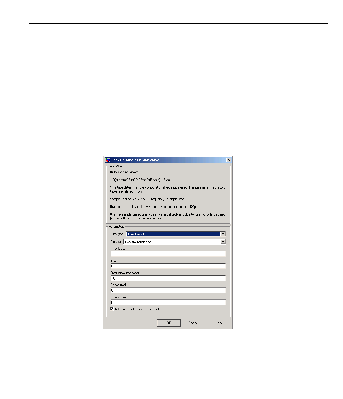
9 Set the block parameters.

a Double-clicktheSineWaveblock.Thedialogboxthatappearsallows

you to set the block’s parameters.

For this example, configure the block to generate a 10 rad/s sine wave by entering default amplitude of

10 for th e Frequency parameter. The sinusoid has the

1 and phase of 0 specified by the Amplitude and

Phase offset parameters.

b Click OK.

c Double-click the Second Order Linear Actuator block.

2-13

2 Using the Aerospace Blockset™ Software

In this example, the actuator has the default natural frequency of 150 rad/s, a damping ratio of 0.7, and an initial position of 0 radians specified by the Natural frequency, Damping ratio,andInitial position parameters.

d Click OK.

Running the Simulation

You can now run the model that you built to see how the system behaves in time:

2-14

1 Double-click the Scope block if the Scope window is not already open on

your screen. The Scope window appears.

2 Select

contai positi

3 Adjust the Scope block’s display. While the simulation is running,

Start from the Simulation menu in the model window. The signal

ning the 10 rad/s sinusoid and the signal containing the actuator

on are plotted on the scope.

right-click the y-axis of the scope and select Autoscale. The vertical range of the scope is adjusted to better fit the signal.

4 Vary the S ine Wave block parameters.

a While the simulation is running, double-click the Sine Wave block to

open its parameter dialog box. This causes the simulation to pause.

b You can then change the frequency of the sinusoid. Try entering 1 or

20 in the Frequency field. Close the Sine Wave dialog box to enter

Building a Simple Actuator System

your change and allow the simulation to continue. You can then observe the changes on the scope.

5 Select Stop from the Simulation menu to stop the simulation.

Many parameters cannot be changed while a simulation is running. This is usually the case for parameters that directly or indirectly alter a signal’s dimensions or sample rate. However, there are some parameters, like the Sine Wave Frequency parameter, that you can tune without stopping the simulation.

Note Opening a dialog box for a source block causes Simulink to pause. While Simulink is paused, you can edit the parameter values. You must close the dialog box to h av e the ch ang es take e ffect and allow Simulink to continue.

Running a Simulation from a MATLAB File

You can also modify and run a Simulink simulation from a MATLAB MATLAB file. By doing this, you can automate the variation of model parameters to explore a large number of simulation conditions rapidly and efficiently. For information on how to do this, see the Simulink documentation.

2-15

2 Using the Aerospace Blockset™ Software

About Aerospace Coordinate Systems

In this section...

“Fundamental Coordinate System Concepts” on page 2-16

“Coordinate Systems for Modeling” on page 2-18

“Coordinate Systems for Navigation” on page 2-20

“Coordinate Systems forDisplay”onpage2-23

“References” on page 2-24

Fundamental Coordinate System Concepts

Coordinate systems a llow you to keep track of an aircraft or spacecraft’s position and orientation in space. The Aerospace Blockset coordinate systems are based on these underlying concepts from geodesy, astronomy, and physics.

Definitions

The blockset uses right-handed (RH) Cartesian coordinate systems. The right-hand rule establishes the x-y-z sequence of coordinate axes.

2-16

An inertial frame is a nonaccelerating motion reference frame. In an inertial frame, Newton’s second law holds: force = mass•acceleration. Loosely speaking, acceleration is defined with respect to the distant cosmos, and an inertial frame is often said to be nonaccelerated with respect to the “fixed stars.” Because the Earth and stars move so slowly with respect to one another, this assumption is a very accurate approximation.

Strictly defined, an inertial frame is a member of the set of all frames not accelerating relative to one another. A noninertial frame is any frame accelerating relative to an inertial frame. Its acceleration, in general, includes both translational and rotational components, resulting in pseudoforces (pseudogravity, as well as Coriolis and centrifugal forces).

The blockset models the Earth’s shape (the geoid) as an oblate spheroid, a special type of ellipsoid with two longer axes equal (defining the equatorial plane) and a third, slightly shorter (geopolar) axis of symmetry. The equator is the intersection of the equatorial plane and the Earth’s surface. The

About Aerospace Coordinate Systems

geographic poles are the intersection o f the Earth’s surface and the geopolar axis. In general, the Earth’s geopo lar and rotation axes are not identical.

Latitudes parallel the equator. Longitudes parallel the geopolar axis. The zero longitude or prime meridian passes through Greenwich, England.

Approximations

The blockset makes three standard approximations in defining coordinate systemsrelativetotheEarth.

• The Earth’s surface or geoid is an oblate spheroid , defined by its lo nger

equatorial and shorter geopolar axes. In reality, the Earth is slightly deformed with respect to the standard geoid.

• The Earth’s rotation axis and equatorial plane are perpendicular, so that

the rotation and geopolar axes are identical. In reality, these axes are slightly misaligned, and the equatorial plane wobbles as the Earth rotates. This effect is negligible in most applications.

• The only noninertial effect in Earth-fixed coordinates is due to the Earth’s

rotation about its axis. Th is is a rotating, geocentric system. The blockset ignores the Earth’s acceleration around the Sun, the Sun’s acceleration in the Galaxy, and the Galaxy’s acceleration through the cosmos. In most applications, only the Earth’s rotation matters.

This approximation must be changed for spacecraft sent into deep space, i.e., outside the Earth-Moon system, and a heliocentric system is preferred.

Motion with Respect to Other Planets

The blockset uses the standard WGS-84 geoid to model the Earth. You can change the equatorial axis length, the flattening, and the rotation rate.

You can represent the motion of spacecraft with respect to any celestial body that is well approximated by an oblate spheroid by changing the spheroid size, flattening, and rotation rate. If the celestial body is rotating westward (retrogradely), make the rotation rate negative.

2-17

2 Using the Aerospace Blockset™ Software

Coordinate Systems for Modeling

Modeling aircraft and spacecraft is simplest if you use a coordinate system fixed in the body itself. In the case of aircraft, the forward d irection is modified by the presence of wind, and the craft’s motion through the air is not the same as its motion relative to the ground.

See the “Equations of Motion” on page 4-7 for further details on how the Aerospace Blockset product implements body and wind coordinates.

Body Coordinates

The noninertial body coordinate system is fixed in both origin and orientation to the moving craft. The craft is assumed to be rigid.

The orientation of the body coordinateaxesisfixedintheshapeofbody.

• The x-axis points through the nose of the craft.

• The y-axis points to the right of the x-axis (facing in the pilot’s direction of

view), perpendicular to the x-axis.

2-18

• The z-axis points down through the bottom the craft, perpendicular to the

xy plane and satisfying the RH rule.

Translational Degrees of Freedom. Translations are defined by moving along these axes by distances x, y,andz from the origin.

Rotational Degrees of Freedom. Rotations are defined by the Euler angles

P, Q, R or Φ, Θ, Ψ.Theyare:

P or Φ

Q or Θ

R or Ψ

Roll about the x-axis

Pitch about the y-axis

Yaw about the z-axis

About Aerospace Coordinate Systems

Wind Coordinates

The noninertial wind coordinate system has its origin fixed in the rigid aircraft. The coordinate system orientation is defined relative to the craft’s velocity V.

The o rientation of the wind coordinate axes is fixed by the velocity V .

• The x-axis points in the direction of V.

• The y-axis points to the right of the x-axis (facing in the direction of V),

perpendicular to the x-axis.

• The z-axis points perpendicular to the xy plane in w hatever way needed to

satisfy the RH rule with respect to the x-andyaxes.

Translational Degrees of Freedom. Translations are defined by moving along these axes by distances x, y,andz from the origin.

Rotational Degrees of Freedom. Rotations are defined by the Euler angles Φ, γ, χ.Theyare:

Bank angle about the x-axis

Flight path about the y-axis

Heading angle about the z-axis

2-19

2 Using the Aerospace Blockset™ Software

Coordinate Systems for Navigation

Modeling aerospace trajectories requires positioning and orienting the aircraft or spacecraft with respect to the rotating Earth. Navigation coordinates are defined with respect to the center and surface of the Earth.

Geocentric and Geodetic Latitudes

The geocentric latitude λ on the Earth’s surface is defined by the angle subtended by the radius vector from the Earth’s center to the surface point with the equatorial plane.

2-20

The geodetic latitude µ on the Earth’s surface is defined by the angle subtended by the surface normal vector n and the equatorial plane.

About Aerospace Coordinate Systems

NED Coordinates

The north-east-down (NED) system is a noninertial system with its origin fixed at the aircraft or spacecraft’s center of gravity. Its axes are oriented along the geodetic directions defined by the Earth’s surface.

• The x-axis points north parallel to the geoid surface, in the polar direction.

• The y-axis points east parallel to the geoid surface, along a latitude curve.

• The z-axis points downward, toward the Earth’s surface, antiparallel to the

surface’s outward normal n.

Flying at a constant altitude means flying at a constant z above the Earth’s surface.

ECI Coordinates

The Earth-centered inertial (ECI) system is a mixed inertial system. It is oriented with respect to the Sun. Its origin is fixed at the center of the Earth. (See figure following.)

• The z-axis points northward along the Earth’s rotation axis.

• The x-axis points outward in the Earth’s equatorial plane exactly at the

Sun. (This rule ignores the Sun’s oblique angle to the equator, which varies with season. The actual Sun always remains in the xz plane.)

2-21

2 Using the Aerospace Blockset™ Software

• The y-axis points into the eastward quadrant, perpendicular to the xz plane

so as to satisfy the RH rule.

2-22

Earth-Centered Coordinates

ECEF Coordinates

The Earth-center, Earth-fixed (ECEF) system is a noninertial system that rotates with the Earth. Its origin is fixed at the center of the Earth. (See figure preceding.)

• The z′-axis points northward along the E arth’s rotation axis.

• The x′-axis points outward along the intersection of the Earth’s equatorial

planeandprimemeridian.

• The y′-axis points into the eastward quadrant, perpendicular to the x-z

planesoastosatisfytheRHrule.

About Aerospace Coordinate Systems

Coordinate Systems for Display

Several display tools are available for use with the Aerospace Blockset product. Each has a specific coordinate system for rendering mo tion.

MATLAB Graphics Coordinates

See the MATLAB 3-D Visualization documentation for more information about the MATLAB Graphics coordinate axes.

MATLAB Graphics uses this default coordinate axis orientation:

• The x-axis points out of the screen.

• The y-axis points to the right.

• The z-axispointsup.

FlightGear Coordinates

FlightGear is an open-source, third-party flight simulator with an interface supported by the blockset.

• “Working with the Flight Simulator Interface” on page 2-32 discusses the

blockset interface to FlightGear.

• See the FlightGear documentation at

information about this flight simulator.

The FlightGear coordinates form a special body-fixed system, rotated from the standard body coordinate system about the y-axis by -180 degrees:

• The x-axis is positive toward the back of the vehicle.

• The y-axis is positive toward the right of the vehicle.

• The z-axis is positive upward, e.g., wheels typically have the lowest z values.

www.flightgear.org for complete

2-23

2 Using the Aerospace Blockset™ Software

AC3D Coordinates

AC3D is a low-cost, widely used, geo metry editor available from

www.ac3d.org. Its body-fixed coordinates are formed by inverting the three

standard body coordinate axes:

• The x-axis is positive toward the back of the vehicle.

• The y-axis is positive upward, e.g., wheels typically have the lowest y

values.

2-24

• The z-axisispositivetotheleftofthevehicle.

References

Recommended Practice for Atmospheric and Space Flight Vehicle Coordinate Systems, R-004-1992, ANSI/AIAA, February 1992.

Mapping Toolbox User’s Guide, The MathWorks, Inc., Natick, Massachusetts.

www.mathworks.com/access/helpdesk/help/toolbox/map/.

About Aerospace Coordinate Systems

Rogers, R. M., Applied Mathematics in Integrated Navigation Systems, AIAA, Reston, Virginia, 2000.

Sobel, D., Longitude, Walker & Company, New Y ork, 1995.

Stevens, B. L., and F. L. Lewis, Aircraft Control and Simulation, 2nd ed., Aircraft Control and Simulation, Wiley-Interscience, New York, 2003.

Thomson, W. T., Introduction to Space Dynamics, John Wiley & Sons, New York, 1961/Dover Publications, Mineola, New York, 1986.

World Geodetic System 1984 (WGS 84),

http://earth-info.nga.mil/GandG/wgs84/.

2-25

2 Using the Aerospace Blockset™ Software

Introducing the Flight Simulator Interface

In this section...

“About the FlightGear Interface” on page 2-26

“Obtaining FlightGear” on page 2-26

“Configuring Your Computer for FlightGear” on page 2-27

“Installing and Starting FlightGear” on page 2-30

About the FlightGear Interface

The Aerospace Blockset product supports an i nterface to the third-party FlightGear flight simulator, an open source software package a vailable through a GNU General Public License (GPL). The FlightGear flight simulator interface included with the blockset is a unidirectional transmission link from the Simulink interface to FlightGear using FlightGear’s published

net_fdm binary data exchange protocol. Data is transmitted via UDP network

packets to a running instance of FlightGear. The blockset supports multiple standard binary distributions of FlightGear. See “Running FlightGear with the Simulink Models” on page 2-38 for interface details.

2-26

FlightGear is a separate software entity neither created, owned, nor maintained by The MathWorks.

• To report bugs in or request enhancements to the

Aerospace Blockset FlightGear interface, use this form

http://www.mathworks.com/contact_TS.html.

• To report bugs or request enhancements to FlightGear itself, visit

www.flightgear.org and use the contact page.

Obtaining FlightGear

You can obtain FlightGear from www.flightgear.org in the download area or by ordering CDs from FlightGear. The dow nload area contains extensive documentation for installation and configu ration. Because FlightGear is an open source project, source downloads are also available for customization and porting to custom environments.

Introducing the Flight Simulator Interface

Configuring Your Computer for F lightGear

You must have a high performance graphics card with stable drivers to use FlightGear. For more information, see the FlightGear CD distribution or the hardware requirements and documentation areas of the FlightGear Web site,

www.flightgear.org.

MathWorks tests of FlightGear’s performance and stability indicate significant sensitivity to computer video cards, driver versions, and driver settings. You need OpenGL The OpenGL settings are particularly important. Withoutpropersetup, performance can drop from about a 3 0 frames-per-second (fps) update rate to less than 1 f ps.

Graphics Recommendations for Windows

The MathWorks recommends the following for Windows users:

• Choose a graphics card with good OpenGL performance.

• Always use the latest tested and stable driver release for your video card.

Test the driver thoroughly on a few computers before deploying to others.

support with hardware acceleration activated.

For Microsoft Windows XP systems running on x86 (32-bit) or AMD-64/EM64T chip architectures, the graphics card operates in the unprotected kernel space known as Ring Zero. This means that glitches in the driver can caus e Windows to lock or crash. Before buying a large number of computers for 3-D applications, test, with your vendor, one or two computers to find a combination of hardware, operating system, drivers, and settings that are stable for your applications.

Setting Up OpenGL Graphics on Windows

For complete information on OpenGL settings, refer to the documentation at the OpenGL Web site:

Follow these steps to optimize your video card settings. Your driver’s panes might look different.

1 Ensure that you have activated the OpenGL hardware acceleration on

your video card. On Windows, access this configuration through Start >

www.opengl.org.

2-27

2 Using the Aerospace Blockset™ Software

Settings > Control Panel > Display, which opens the following dialog box. Select the Settings tab.

2-28

2 Click the Advanced button in the lower right of the dialog box, which

brings up the graphics card’s custom configuration dialog box, and go to the OpenGL tab. For an ATI Mobility Radeon 9000 video card, the OpenGL pane looks like this:

Introducing the Flight Simulator Interface

3 For best performance, move the Main Settings slider near the top of the

dialog box to the Performance end of the slider.

4 If stability is a problem, try other screen resolutions, other color depths in

the Displays pane, and other OpenGL acceleration modes.

Many cards perform m uch better at 16 bits-per-pixel color depth (also known as 65536 color mode, 16-bit color). For example, on an ATI Mobility Radeon 9000 running a given model, 30 fps are achieved in 16-bit color mode, while 2 fps are achieved in 32-bit color mode.

Setup on Linux, Macintosh, and Other Platforms

FlightGear distributions are available for Linux®,Macintosh®, and other UNIX platforms from the FlightGear Web site, Installation on these platforms, like Windows, requires careful configuration of graphics cards and drivers. Consult the documentation and hardware requirements sections at the FlightGear Web site.

www.flightgear.org.

2-29

2 Using the Aerospace Blockset™ Software

UsingMATLABGraphicsControlstoConfigureYourOpenGL Settings

You can also control your OpenGL rendering from the MATLAB command line with the MATLAB Graphics command reference for more information.

Installing and Starting FlightGear

The extensive FlightGear documentation guides you through the installation in detail. Consult the documentation section of the FlightGear Web site for complete installation instructio n s:

Keep the following points in mind:

• Generous central processor speed, system and video R AM, and virtual

memory are essential for good flight simulator performance.

The MathWorks recommends a minimum of 512 megabytes of system RAM and 128 megabytes o f video RAM for reasonable performance.

opengl command. Consult the opengl

www.flightgear.org.

2-30

• Be sure to have sufficient disk space for the FlightGear download a nd

installation.

• The MathWorks recommends configuring your computer’s graphics card

before you install FlightGear. See the preceding section, “Configuring Your Computer for FlightGear” on page 2-27.

• Shutting down all running applications (including the MATLAB interface)

before installing FlightGear is recommended.

• MathWorks tests indicate that the operational stability of FlightGear

is especially sensitive during startup. It is best to not move, resize, mouse over, overlap, or cover up the FlightGear window until the initial simulation scene appears after the startup splash screen fades out.

• The current releases of FlightGear are optimized for flight visualization at

altitudes below 100,000 feet. FlightGear does work not well or at all with very high altitude and orbital views.

Aerospace Toolbox supports FlightGear on a number of platforms (

http://www.mathworks.com/products/aerotb/requirements.html). The

following table lists the properties you should be aware of before you start to use FlightGear.

Introducing the Flight Simulator Interface

FlightGear Property

FlightGearBaseDirectory

GeometryModelName

Folder Description

FlightGear installation folder.

Model geometry folder

Platforms

Windows

Solaris™ or Linux

Mac

Windows

Solaris or Linux

Mac

Typica l Lo cation

C:\Program Files\FlightGear

(default)

Folder into whichyouinstalled FlightGear

/Applications

(directory to which you dragged the FlightGear icon)

C:\Program Files\FlightGear\data\Aircraft\HL20

(default)

$FlightGearBaseDirectory/data/Aircraft/HL20

$FlightGearBaseDirectory/FlightGear.app/Contents/Resources/data/Aircraft/HL20

2-31

2 Using the Aerospace Blockset™ Software

Working with the Flight Simulator Interface

In this section...

“Introduction” on page 2-32

“About Aircraft Geometry Models” on page 2-33

“Working w ith Aircraft Geometry Models” on page 2-35

“Running FlightGear with the Simulink Models” on page 2-38

“Running the NASA HL-20 Demo with FlightGear” on page 2-48

Introduction

Use this section to learn how to use the FlightGear flight simulator and the Aerospace Blockset software to visualize your Simulink aircraft models. If you have not yet installed FlightGear, see “Introducing the Flight Simulator Interface” on page 2-26 first.

2-32

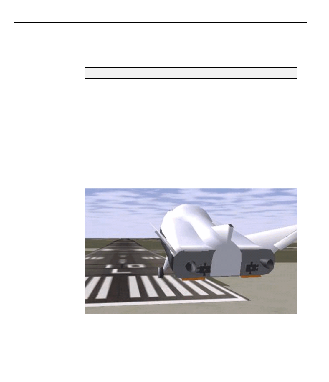
Simulink®Driven HL-20 Model in a Landing Flare at KSFC

Working with the Flight Simulator Interface

About A ircraft Geometry Models

Before you can visualize your aircraft’s dynamics, you need to create or obtain an aircraft model file compatible with FlightGear. This section explains h ow to do this.

Aircraft Geometry Editors and Formats

Youhaveacompetitivechoiceofovertwelve3-Dgeometryfileformats supported by FlightGear.

Currently, the most popular 3-D geometry file format is the AC3D form a t, which has the suffix

www.ac3d.org. Another popular 3-D editor for aircraft models is Flight Sim

Design Studio, distributed by A ba c us Pu blications at

Aircraft Model Structure and Requirements

Aircraft models are contained in the FlightGearRoot/data/Aircraft/ folder and subfolders. A complete aircraft model must contain a folder linked through the required aircraft master file named

*.ac. AC3D is a low-cost geometry editor available from

www.abacuspub.com.

model-set.xml.

Allothermodelelementsareoptional. Thisisapartiallistoftheoptional elements you can put in an aircraft data folder:

• Vehicle objects and their shapes and colors

• Vehicle objects’ surface bitmaps

• Variable geometry descriptions

• Cockpitinstrument3-Dmodels

• Vehicle sounds to tie to events (e.g., engine, gear, wind noise)

• Flight dynamics model

• Simulator views

• Submodels (independently movable items) associated with the vehicle

Model behavior reverts to defaults when these elements are not used. For example,

• Default sound: no vehicle-related sounds are emitted.

2-33

2 Using the Aerospace Blockset™ Software

• Default instrument panel: no instruments are shown.

Models can contain some, all, or even none of the above elements. If you always run FlightGear from the cockpit view, the aircraft geometry is often secondary to the instrument geometries.

A how-to document for including optional elements is included in the FlightGear documentation at:

http://www.flightgear.org/Docs/fgfs-model-howto.html

Required Flight Dynamics Model Specification

The flight dyna mics model (FDM) specification is a required element for an aircraft model. To set the Simulink software as the source of the flight dynamics m odel data s tre am for a given geometry model, you put this line in

data/Aircraft/model/model-set.xml:

<flight-model>network</flight-model>

2-34

Obtaining and Modifying Existing Aircraft Models

You can quickly build models from scratch by referencing instruments, sounds, and other optional elements from existing FlightGear models. Such models provide examples of geometry, dynamics, instruments, views, and sounds. It is simple to copy an aircraft folder to a n ew name, rename the

model-set.xml file, modify it for network flight dynamics, and then run

FlightGear with the

Many existing 3-D aircraft geometry models are available for use with FlightGear. Visit the download area of the aircraft models available. Additional models can be obtained via Web search. S earch key words such as “flight gear aircraft model” are a good starting point. Be sure to comply with copyrights when distributing these files.

aircraft flag set to the name in model-set.xml.

www.flightgear.org toseesomeof

Hardware Requirements for Aircraft Geometry Rendering

When creating your own geometry files, keep in mind that your graphics card can efficiently render a limited number of surfaces. Some cards can efficiently render fewer than 1000 surfaces with bitmaps and specular reflections at

Working with the Flight Simulator Interface

the nominal rate of 30 frames per second. Other cards can easily render on the order of 10,000 surfaces.

If your performance slows while using a particular geometry, gauge the effect of geometric complexity on graphics performance by varying the number of aircraft model surfaces. An easy way to check this is to replace the full aircraft geometry file with a simple shape, such as a single triangle, then test FlightGear with this simpler geometry. If a geometry file is too complex for smooth display, use a 3-D geometry editor to simplify your model by reducing the number of surfaces in the geometry.

Working with Aircraft Geometry M odels

Once you have obtained, modified, or created an aircraft data file, you need to put it in the correct folder for FlightGear to access it.

Importing Aircraft Models into FlightGear

To install a compatible model into FlightGear, use one of the following procedures. Choose the one appropriate for your platform. This section assumes that you have read “Installing and Starting FlightGear” on page 2-30.

If your platform is Windows:

1 Go to your installed FlightGear folder. O pen the data folder, then the

Aircraft folder: \FlightGear\data\Aircraft\.

2 Make a subfolder model\ here for your aircraft data.

3 Put model-set.xml in that subfolder, plus any other files needed.

It is common practice to make subdirectories for the vehicle geometry files (

\model\), instruments (\instruments\), and sounds (\sounds\).

If your platform is UNIX or Linux:

1 Go to your installed FlightGear directory. Open the data directory, then

the

Aircraft directory: $FlightGearBaseDirectory/data/Aircraft/.

2 Make a subdirectory model/ here for your aircraft data.

2-35

2 Using the Aerospace Blockset™ Software

3 Put model-set.xml in that subdirectory, plus any other files needed.

It is common practice to make subdirectories for the vehicle geometry files (

/model/), instruments (/instruments/), and sounds (/sounds/).

If your platform is Mac:

1 Open a terminal.

2 Go to your installed FlightGear folder. O pen the data folder, then the

Aircraft folder:

$FlightGearBaseDirectory/FlightGear.app/Contents/Resources/data/Aircraft/

3 Make a subfolder model/ here for your aircraft data.

4 Put model-set.xml in that subfolder, plus any other files needed.

It is common practice to make subdirectories for the vehicle geometry files (

/model/), instruments (/instruments/), and sounds (/sounds/).

2-36

Example: Animating Vehicle Geometries

This example illustrates how to prepare hinge line definitions for animated elements such as vehicle control surfaces and lan d ing gear. To enable animation, each element must be a named entity in a geometry file. The resulting code forms part of the HL20 lifting body model presented in “Running the NASA HL-20 Demo with FlightGear” on page 2-48.

1 The standard body coordinates used in FlightGear geometry models form a

right-handed system, rotated from the standard body coordinate system in Y by -180 degrees:

• X = positive toward the back of the v ehicle

• Y = positive toward the right of the vehicle

• Z = positive is up, e.g., wheels typical ly have the lowest Z values.

See “About Aerospace Coordinate Systems” on page 2-16 for more details.

Working with the Flight Simulator Interface

2 Find two points that lie on the desired named-object hinge line in body

coordinates and write them down as XYZ triplets or put them into a MATLAB calculation like this:

a = [2.98, 1.89, 0.53]; b = [3.54, 2.75, 1.46];

3 Calculate the difference between the points:

pdiff = b - a pdiff =

0.5600 0.8600 0.9300

4 The hinge point is either of the points in step 2 (or the midpoint as shown

here):

mid = a + pdiff/2 mid =

3.2600 2.3200 0.9950

5 Put the hinge point into the animation scope in model-set.xml:

<x-m>3.26</x-m> <y-m>2.32</y-m> <z-m>1.00</z-m>

</center>

6 Use the difference from step 3 to define the relative motio n vector in the

animation axis:

<axis>

</axis>

7 Put these steps together to obtain the complete hinge line animation used

in the HL20 demo model:

2-37

2 Using the Aerospace Blockset™ Software

<type>rotate</type>

<property>/surface-positions/right-aileron-pos-norm</property>

<offset-deg>0</offset-deg>

<x-m>3.26</x-m>

<y-m>2.32</y-m>

<z-m>1.00</z-m>

</center>

<axis>

</axis>

</animation>

Running FlightGear with the Simulink Models

To run a Simulink model of your aircraft and simultaneously animate it in FlightGear with an aircraft data file the aircraft data file and modify your Simulink model with some new blocks.

model-set.xml, you need to configure

2-38

These are the m ain steps to connecting and using FlightGear with the Simulink software:

• “Setting the Flight Dynamics Model to Network in the Aircraft Data File”

on page 2-39 explains how to create the network connection you need.

• “Obtaining the Destination IP Address” on page 2-39 starts by determining

the IP address of the computer running FlightGear.

• “Adding and Connecting Interface Blocks” on page 2-40 shows how to add

and connect interface and pace blocks to your Simulink model.

• “Creating a FlightGear Run Script” on page 2-43 shows how to write a

FlightGear run script compatible with your Simulink model.

• “Starting FlightGear” on page 2-45 guides you through the final steps to

making the Simu link software work with FlightGear.

• “Improving Performance” on page 2-47 helps you speed your model up.

Working with the Flight Simulator Interface

• “Running FlightGear and Simulink Software on Different Computers” on

page 2-47 explains how to connect a simulation from the Simulink software running on one computer to FlightGear running on another computer.

Setting the Flight Dynamics Model to Network in the Aircraft Data File

Be sure to

• Remove any pre-existing flight dynamics model (FDM) data from the

aircraft data file.

• Indicate in the aircraft data file that its FDM is streaming from the

network by adding this line:

<flight-model>network</flight-model>

Obtaining the Destination IP Address

You need the destination IP address for your Simulink model to stream its flight data to FlightGear.

• If you know your computer’s name, enter at the MATLAB command line:

java.net.InetAddress.getByName('www.mathworks.com')

• If you are running FlightGear and the Simulink software on the same

computer, get your computer’s name by entering at the MATLAB command line:

java.net.InetAddress.getLocalHost

• If you are working in Windows, get your computer’s IP address by entering

at the DOS prompt:

ipconfig /all

Examine the IP address entry in the resulting output. There is one entry per Ethernet device.

2-39

2 Using the Aerospace Blockset™ Software

Adding and Connecting Interface Blocks

The easiest way to connect your model to FlightGear with the blockset is to use the FlightGear Preconfigured 6DoF Animation block:

FlightGear Preconfigured 6DoF Animation Block

2-40

The FlightGear Preconfigured 6DoF Animation block is a subsystem containing the Pack net_fdm Packet for FlightGear and Send net_fdm Packet to FlightGear blocks:

Working with the Flight Simulator Interface

Send net_fdm Packet to FlightGear

Pack net_fdm Packet to FlightGear

These blocks transmit data to a FlightGear session. The blocks are separate for maximum flexibility and compatibility.

• The Pack n et_fdm Packet for FlightGear block formats a binary

structure compatible with FlightGear from model inputs. In the default configuration, the block displays only the 6DoF ports, but you can configure the full FlightGear interface supporting more than 50 distinct signals from the block dialog box:

2-41

2 Using the Aerospace Blockset™ Software

2-42

• The Send net_fdm Packet to FlightGear block transmits this packet via

UDP to the specified IP address and port w here a FlightGear session awaits an incoming datastream. Use the IP address you found in “Obtaining the Destination IP Address” on page 2-39.

• The Simulation Pace bl o ck, available in the “Animation Support Utilities

Sublibrary” on page 2-5, slows the simulation so that its aggregate run rate is 1 second of simulation time per second of clock time. You can also use it to specify other ratios of simulation time to clock time.

Working with the Flight Simulator Interface

Simulation Pace

Creating a FlightGear Run Script

To start FlightGear with the desired initial conditions (location, date, time, weather, operating modes), it is best to create a run script by “Using the Generate Run Script Block” on page 2-43 or “Using the Interface Provided with FlightGear” on page 2-45.

If you make separate run scripts f or each model you intend to link to FlightGear and place them in separate directories, run the appropriate script from the MATLAB interface just before starting your Simulink model.

Using the Generate Run Script Block. Theeasiestwaytocreatearun script is by using the Generate Run Script block. Use the following procedure:

1 Open the “Flight Simulator Interfaces Sublibrary” on page 2-5.

2 Create a new Simulink mode l or open an existing model.

3 Drag

4 Double-click the Generate Run Script block. Its dialog opens.

a G enerate Run Script block into the Simulink diagram.

2-43

2 Using the Aerospace Blockset™ Software

2-44

5 In the Output file name field, type the name of the output file. This name

should be the name of the command, with the use to start FlightGear with these initial parameters.

xample, if your filename is

For e

ute the run script and start FlightGear.

exec

6 In the FlightGear base directory field, specify the name of your

FlightGear installation folder.

runfg.bat,usetherunfg command to

.bat extension, you want to

Working with the Flight Simulator Interface

7 In the FlightGear geometry model name field, specify the name of

the subfolder, in the

FlightGear/data/Aircraft folder, containing the

desired model geometry.

8 Specify the initial conditions as needed.

9 Click the Generate Script button at the top of the Parameters area.

The Aerospace Blockset software generates the run script, and saves it in your MATLAB working folder under the filename that you spec if ied in the Output file name field.

10 Repeat steps 5 through 9 to generate other run scripts, if needed.

11 Click OK to close the dialog box. You do not need to save the Generate Run

Script block with the Simulink model.

The Generate Run Script block saves the run script as a tex t file in your working folder. This is an example of the contents of a run script file:

>> cd D:\Applications\FlightGear-1.9.1

>> SET FG_ROOT=D:\Applications\FlightGear-1.9.1\data

>> cd \bin\Win32\

>> fgfs --aircraft=HL20 --fdm=network,localhost,5501,5502,5503

--fog-fastest --disable-clouds --start-date-lat=2004:06:01:09:00:00

--disable-sound --in-air --enable-freeze --airport=KSFO --runway=10L

--altitude=7224 --heading=113 --offset-distance=4.72 --offset-azimuth=0

Using the Interface Provided with FlightGear. The FlightGear launcher GUI (part of FlightGear, not the Aerospace Blockset product) lets you build simple and advanced options into a visible FlightGear run command.

Starting FlightGear

If your computer has enough computational power to run both the Simulink software and FlightGear at the same time, a simple way to start FlightGear on a Windows system is to create a MATLAB desktop button containing the following command to execute a run script like the one created above:

system('runfg &')

To create a desktop button:

2-45

2 Using the Aerospace Blockset™ Software

1 From the Start button on your MATLAB desktop, click Shortcuts > New

Shortcut.TheShortcut Editor dialog opens.

2 Set the Label, Callback, Category,andIcon fields as shown in the

following figure.

3 Click Sav

The FlightGear toolbar button appears in your MATLAB desktop. If you click it, the

runfg.bat file runs in the current folder.

FlightGear button

Once you have completed the s etup, start FlightG ear and run your model:

1 Make sure your model is in a writable folder. Open the model, and update

the diagram. This step ensures that any referenced block code is compiled and that the block diagram is compiled before running. Once you start FlightGear, it uses all available processor power while it is running.

2 Click the FlightGear button or run the FlightGear run script manually.

2-46

Working with the Flight Simulator Interface

3 When FlightGear starts, it displays the initial view at the initial

coordinates specified in the run script. If you are running the Simulink software and FlightGear on different computers, arrange to view the two displays at the same time.

4 Now begin the simulation and v iew the animation in FlightG e ar.

Improving Performance

If your Simulink model is complex and cannot run at the aggregate rate needed for the visualization, you might need to

• Use the Accelerator mode in Simulink (“Accelerating Models” i n Simulink

User’s Guide) to speed up your model execution.

• Free up processor power by running the Simulink model on one computer

and FlightGear on another computer. Use the Destination IP Address parameter of the Send net_fdm Packet to FlightGear block to specify the network address of the computer w here FlightGear is running.

• Simulate the Simulink model first, then save the resulting translations

(x-axis, y-a xis, z-axis) and positions (latitude, longitude, altitude ), and use the FlightGear Animation object in Aerospace Toolbox to visualize this data.

Running FlightGear and Simulink Software on Different Computers

ItispossibletosimulateanaerospacesystemintheSimulinkenvironment on one computer (the source) and use its simulation output to animate FlightGear on another computer (the target). The steps are similar to those already explained, with certain modifications.

1 Obtain the IP address of the com puter running FlightGear. See “Obtaining

the Destination IP Address” on pa ge 2-39.

2 Enter this target computer’s IP address in the Send net_fdm Packet to

FlightGear block. See “Adding and Connecting Interface Blocks” on page 2-40.

2-47

2 Using the Aerospace Blockset™ Software

3 Update the Generate Run Script block in your model with the target

computer’s FlightGear base folder. Regenerate the run script to reflect the target computer’s separate identity.

See “Creating a FlightGear Run Script” on page 2-43.

4 Copy the generated run script to the target computer. Start FlightGear

there. See “Starting FlightGear” on page 2-45.

5 Start your Simulink model on the source computer. FlightGear running on

the target displays the simulation motion.

Running the NASA HL-20 Demo with FlightGear

The Aerospace Blockset software contains a demo model of the NASA HL-20 lifting body that uses the FlightGear interface.

YouneedtohaveFlightGearinstalledand configured before attempting to simulate this model. See “Introducing the Flight Simulator Interface” on page 2-26. This section assumes that you have read “Installing and Starting FlightGear” on page 2-30. Before you start, perform the following, depending on your platform.

2-48

Windows

Copy the

HL20 folder from matlabroot\toolbox\aeroblks\aerodemos\

folder to FlightGear\data\Aircraft\ folder. This folder contains the preconfigured geometries for the HL-20 simulation and

matlabroot\toolbox\aeroblks\aerodemos\HL20\models\HL20.xml

HL20-set.xml.Thefile

defines the geometry.

For more about this step, see “Im porting Aircraft Models into FlightGear” on page 2-35.

UNIX/Linux

Copy the

matlabroot/toolbox/aeroblks/aerodemos/ directory to $FlightGearBaseDirectory/data/Aircraft/ directory.

HL20 directory from

This directory contains the preconfigured geometries for the HL-20 simulation and

HL20-set.xml.Thefile

Working with the Flight Simulator Interface

matlabroot/toolbox/aeroblks/aerodemos/HL20/models/HL20.xml

defines the geometry.

For more about this step, see “Im porting Aircraft Models into FlightGear” on page 2-35.

Mac

Copy the

matlabroot/toolbox/aeroblks/aerodemos/ folder to $FlightGearBaseDirectory/FlightGear.app/Contents/Resources/-

data/Aircraft/

geometries for the HL-20 simulation and

matlabroot\toolbox\aeroblks\aerodemos\HL20\models\HL20.xml

HL20 folder from

folder. This folder contains the preconfigured

HL20-set.xml.Thefile

defines the geometry.

For more about this step, see “Im porting Aircraft Models into FlightGear” on page 2-35.

1 Start the MATLAB interface. Open the demo either by entering asbhl20

in the MATLAB Command Window or by finding the demo entry (NASA HL-20 with FlightGear Interface) in Aerospace Blockset > Demos and clicking Open this model on its demo page. The model opens.

2-49

2 Using the Aerospace Blockset™ Software

2 If this is your first time running FlightGear for this model, double-click the

Generate Run Script block to create a run script. Make sure to specify your FlightGear installation folder in the FlightGear base directory field. For more information, see “Creating a FlightGear Run Script” on p age 2-4 3.

3 Execute the script you just created manually by entering the following at

the MATLAB command line:

dos('runfg &')

If you created a FlightGear desktop button, you can click it instead to start the run script and start FlightGear. For more information, see “Starting FlightGear” on page 2-45.

4 Now start the simulation and view the animation in FlightGear.

Note With the FlightGear window in focus, press the V key to alternate

between the different aircraft views: cockpit view, helicopter view, chase view, and so on.

2-50

Case Studies

• “Ideal Airspeed Correction” on page 3-2

• “1903 Wright Flyer” on page 3-9

• “NASA HL-20 Lifting Body Airframe” on page 3-19

• “Missile Guidance System” o n page 3-34

3 Case Studies

Ideal Airspeed Correction

In this section...

“Introduction” on page 3-2

“Airspeed Correction Models” on page 3-2

“Measuring Airspeed” on page 3-3

“Modeling Airspeed Correction” on page 3-5

“Simulating Airspeed Correction” on page 3-7

Introduction

This case study simulates indicated and true airspeed. It constitutes a fragment of a complete aerodynamics problem, including only measurement and calibration.

Airspeed Correction Models

To view the airspeed correction models, enter the following at the MATL AB command line:

3-2

aerobl aerob

k_indicated

lk_calibrated

aeroblk_indicated Model

Ideal Airspeed Correction

aeroblk_calibrated Model

Measuring Airspeed

To measure airspeed, most light aircraft designs implement pitot-static airspeed indicators based on Bernoulli’s principle. Pitot-static airspeed indicators measure airspeed by an expandable caps ule that expands and contracts with increasing and decreasingdynamicpressure. Thisisknownas calibrated airspeed (CAS). It is what a pilot sees in the cockpit of an aircraft.

3-3

3 Case Studies

To compensate for measurement errors , it helps to distinguish three types of airspeed. These type s are explained more completely in the following.

Airspeed Type Description

Calibrated Indicated airspeed corrected for calibration

error

Equivalent

True

Calibrated airspeed corrected for compressibility error

Equivalent airspeed corrected for density error

Calibration Error

An airspeed sensor features a static vent to maintain its internal pressure equal to atmospheric pressure. Position and placement of the static vent with respect to the angle of attack and velocity of the aircraft determines the pressure inside the airspeed sensor and therefore the calibration error. Thus, a calibration error is specific to an aircraft’s design.

An airspeed calibration table, which is usually included in the pilot operating handbook or other aircraft documentation, helps pilots convert the indicated airspeed to the calibrated airspeed.

Compressibility Error

The density of air is n ot constant, and the compressibility of air increases with altitude and airspeed, or when contained in a restricted volume. A pitot-static airspeed sensor contains a res tricted volume of air. At high altitudes and high airspeeds, calibrated airspeed is always higher than equivalent airspeed. Equivalent airspeed can be derived by adjusting the calibrated airspeed for compressibility error.

3-4

Density Error

At high altitudes, airspeed indicators read lower than true airspeed because the air density is lower. True airspeed represents the compensation of equivalent airspeed for the density error, the difference in air density at altitude from the air density at sea level, in a standard atmosphere.

Ideal Airspeed Correction

Modeling Airspe

The aeroblk_ind true airspeed an aCessna150MCo implements a co model impleme

Each model con

• “COESA Atmos

atmospheric

• “Ideal Airs

calibrated

icated

d correct it to indicated airspeed for ins trument display in

nversion to indicated airspeed. The

nts a conversion to true airspeed.

sists of two main components:

conditions with changing altitude.

peed Correction Block” on page 3-5 transforms true airspeed to airspeed and vice versa.

ed Correction

and aeroblk_calibrated models show how to take

mmuter light aircraft. The

phere Model Block” on page 3-5 calculates the change in

COESA Atmosphere Model Block

The COESA A of the U.S Atmosphe pressure 32,000 m with the Organiz

ation).

tmosphere Model block is a mathematical representation

. 1976 COESA (Committee on Extension to the Standard

re) standard lower atmospheric values for absolute temperature,

, density, and speed of sound for input geopotential altitude. Below

eters (104,987 fee t), the U.S. Standard Atmosphere is identical Standard Atmosphere of the ICAO (International Civil Aviation

aeroblk_indicated model

aeroblk_calibrated

The

aer

Atmosp for the

oblk_indicated

here Mo del block to supp ly the spe ed of soun d and a ir pressure inputs

Ideal Airspeed Correction block in each model.

and aeroblk_calibrated models use the COESA

Ideal Airspeed Correction Block

The Id erro cont

eal Airspeed Correction block compensates for airspeed measurement

rs to convert airspeed from one type to another type. The following table

ains the Ideal A irspeed Correction block’s inputs and outputs.

Airspeed Input Airspeed Output

ivalent airspeed

True Airspeed

Equ

librated airspeed

3-5

3 Case Studies

Airspeed Input Airspeed Output

Equivalent Airspeed

True airspeed

Calibrated airspeed

Calibrated Airspeed

True airspeed

Equivalent airspeed

In the aeroblk_indicated model, the Ideal Airspeed Correction block transforms true to calibrated airspeed. In the

aeroblk_calibrated model,

the Ideal Airspeed Correction block transforms calibrated to true airspeed.

The following sections explain how the Ideal Airspeed Correction block mathematically represents airspeed transformations:

• “True Airspeed Implementation” on page 3-6

• “Calibrated Airspeed Implementation” on page 3-6

• “Equivalent Airspeed Im plementation” on page 3-7

True Airspeed Implementation. True airspeed (TAS) is implemented as an

input and as a function of equivalent airspeed (EAS), expressible as

EAS a

TAS



3-6

where

Speed of sound at altitude in m/s

Relative pressure ratio at altitude

Speed of sound at mean sea level in m/s

Calibrated Airspeed Implementation. Calibrated airspeed (CAS), derived using the compressible form of Bernoulli’s equation and assuming isentropic conditions, can be expressed as

where

Ideal Airspeed Correction

Air density at mean sea level in kg/m

Static pressure at mean sea level in N/m

Ratio of s pecific heats

Dynamic pres

sure at mean sea level in N/m

Equivalent Airspeed Implementation. Equivalent airspeed (EAS) is the same as CAS, except static pressure at sea level is replaced by static pressure at altitude.

The symbols are defined as follows:

Air density at mean sea level in kg/m

Static pressure at altitude in N/m

Ratio of specific heats

Dynam

ic pressure at mean sea level in N/m

Simulating Airspeed Correction

In the aeroblk_indicated model, the aircraft is defined to be traveling at a constant speed of 72 knots (true airspeed) and altitude of 500 feet. The flaps are set to 40 degrees. The COESA A tmosphere Model block takes the altitude as input and outputs the speed of sound and air pressure. Taking the s pe ed of sound, air pressure, and airspeed as inputs, the Ideal Airspeed Correction block converts true airspeed to calibrated airspeed. Finally, the Calculate IAS subsystem uses the flap setting and calibrated airspeed to calculate indicated airspeed.

3-7

3 Case Studies

The m odel’s Display block shows both indicated and calibrated airspeeds.

In the aero aconstant The flaps the altit

Calculat

to calcul air pres Correct

The mod

ude as input and outputs the speed of sound and air pressure. The

eCAS

ate the calibrated airspeed. Finally, using the speed of sound,

sure, and true calibrated airspeed as inputs, the Ideal Airspeed

ion block converts calibrated airspeed back to true airspeed.

el’s Display block shows both calibrated and true airspeeds.

blk_calibrated

speed of 70 knots (indicated airspeed) and altitude of 500 feet.

are set to 10 degrees. The COESA Atmosphere Model block takes

subsystem uses the flap setting and indicated airspeed

model, the aircraft is defined to be traveling at

3-8

1903 Wright Flyer

In this section...

“Introduction” on page 3-9

“Wright Flyer Model” on page 3-10

“AirframeSubsystem”onpage3-10

“Environment Subsystem” on page 3-14

“Pilot Subsystem” on page 3-15

“Running the Simulation” on page 3-16

“References” on page 3-17

Introduction

Note The final section of this study requires the Simulink 3D An imation

software.

1903 Wright Flyer

This case study describes a model of the 1903 Wright Flyer. Built by Orville and Wilbur Wright, the Wright Flyer took to the skies in December 1903 andopenedtheageofcontrolledflight. TheWrightbrothers’flyingmachine achieved the following goals:

• Left the ground under its own power

• Movedforwardandmaintaineditsspeed

• Landed at an elevation no lower than where it started

This model is based on an earlier simulation [1] that ex plored the longitudinal stability of the Wright Flyer and therefore modeled o nly forward and vertical motion along with the pitch angle. The Wright Flyer suffered from numerous engineering challenges, including dynamic and static instability. Laterally, the Flyer tended to overturn in crosswinds and gusts, and longitudinally, its pitch angle would undulate [2].

3-9

3 Case Studies

Under these constraints, the model recreates the longitudinal f light dynamics that pilots of the Wright Flyer would have experienced. Because they were able to control lateral motion, Orville and Wilbur Wright were able to maintain a relatively straight flight path.

Note, running this model generates assertion messages in the MATLAB Command Window. This is because the model illustrates the use of the Assertion block to indicate that the flyer is hitting the ground when landing.

Wright Flyer Model

Open the Wright Flyer model by entering aeroblk_wf_3dof at the MATLAB command line.

3-10

rame Subsystem

Airf

irframe subsystem simulates the rigid body dynamics of the Wright

The A

er airframe, including elevator angle of attack, aerodynamic coefficients,

Fly

ces and moments, and three-degrees-of-freedom equations of motion.

for

The Airframe subsystem consists of the following parts:

• “Elevator Angle of Attack Subsystem” on page 3-11

1903 Wright Flyer

• “Aerodynamic Coefficients Subsystem” on page 3-12

• “Forces and Moments Subsystem” on page 3-12

• “3DoF (Body Axes) Block” on page 3-13

Elevator Angle of Attack Subsystem

The Elevator Angle of Attack subsystem calculates the effective elevator angle fortheWrightFlyerairframeandfeeds its output to the Pilot subsystem.

3-11

3 Case Studies

Aerodynamic Coefficients Subsystem

The Aerodynamic Coefficie nts subsystem contains aerodynamic data and equations for calculating the aerodynamic coefficients, which are summed and passed to the Forces and Moments subsystem. Stored in data sets, the aerodynamic coefficients are determined by interpolation using Prelookup blocks.

3-12

Forces and Moments Subsystem

The aerodynamic forces and moments acting on the airframe are generated from aerodynamic coefficients. The Forces and Moments subsystem calculates the body forces and body moments acting on the airframe about the center of gravity. These forces and moments depend on the aerodynamic coefficients, thrust, dynamic pressure, and reference airframe parameters.

1903 Wright Flyer

3DoF (Body Axes) Block

The 3DoF (Body Axes) block use equations of motion to define the linear and angular motion of the Wright Flyer airframe. It also performs conversions from the original model’s axis system and the body axes.

3-13

3 Case Studies

3-14

3DoF (Body Axes) Block Parameters

Environment Subsystem

The first and final flights of the Wright Flyer occurred on December 17, 1903. Orville and Wilbur Wright chose an area near Kitty Hawk, North Carolina, situated near the Atlantic coast. Wind gusts of more than 25 miles per hour were recorded that day. After the final flight on that blustery December day, a wind gust caught and ov erturned theWrightFlyer,damagingitbeyond repair.

The Environment subsystem of the Wright Flyer model contains a variety of blocks from the Environment sublibrary of the Aerospace Blockset software, including wind, atmosphere, and gravity, and calculates airspeed and

1903 Wright Flyer

dynamic pressure. The Discrete Wind Gust Model block provides wind gusts to the simulated environment. The other blocks are

• The Incidence & Airspeed block calculates the angle of attack and airspeed.

• The COESA Atmosphere Model block calculates the air density.

• The Dynamic Pressure block computes the dynamic pressure from the air

density and velocity.

• The WGS84 Gravity Model block pro du ce s the gravity at the W righ t Flyer’s

latitude, longitude, and height.

Pilot Subsystem

The Pilot subsystem controls the aircraft by responding to both pitch angle (attitude) and angle of attack. If the angle of attack differs from the set angle of attack by more than one degree, thePilotsubsystemrespondswitha correction of the elevator (canard) angle. When the angular velocity exceeds +/- 0.02 rad/s, angular velocity and angular acceleration are also taken into consideration with add iti onal c orrections to the elevator an gle.

Pilot reaction time largely determined the success of the flights [1]. Without an automatic controller, a reaction time of 0.06 seconds is optimal for successful flight. The D elay of Pilot (VariableTimeDelay)block recreates this effect by producing a delay of no more than 0.08 second.

3-15

3 Case Studies

Running the Simulation

The default values for this simulation allow the Wright Flyer model to take off and land successfully. The p ilot reaction time ( the desired angle of attack ( is low. The Wright Flyer model reacts similarly to the actual Wright Fly er. It leaves the ground, moves forward, and lands on a point as high as that from which it started. This model exhibits the longitudinal undulation in attitude of the o riginal aircraft.

wf_alphaa) is constant, and the altitude attained

wf_B3) is set to 0.06 seconds,

3-16

Attitude Scope (Measured in Radians)

A pilot with quick reaction times and ideal flight conditions makes it possible to fly the Wright Flyer successfully. The Wright Flyer model confirms that

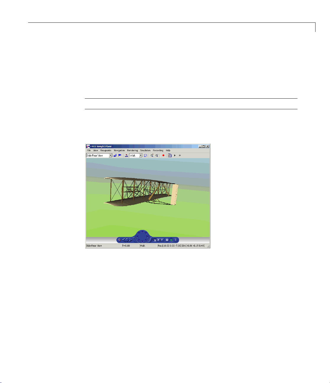
1903 Wright Flyer

controlling its longitudinal motion was a serious challenge. The longest recorded flight on that day lasted a mere 59 seconds and covered 852 feet.

Virtual Reality Visualization of the Wright Flyer

Note This section requires the Simulink 3D Animation.

The Wright Flyer model also provides a virtual world visualization, coded in Virtual Reality Modeling Language (VRML) [3] . The VR Sink block in the main model allows you to view the flight motion in three dimensions.

1903 Wright Flyer V ir tual Reality World

References

[1] Hooven, Frederick J., “Longitudinal Dynamics of the Wright Brothers’ Early Flyers: A Study in Computer Simulation of Flight,” from The Wright Flyer: An Engineering Perspective, ed. Howard S. Wolko, Smithsonian Institution Press, 1987.

3-17

3 Case Studies

[2]Culick,F.E.C.andH.R.Jex,“Aerodynamics,Stability,andControlof the 1903 Wright Flyer,” from The Wright Flyer: An Engineering Perspective, ed. H oward S. Wolko, Smithsonian Institution Press, 1987.

[3] Thaddeus Beier created the initial Wright Flyer model in Inventor format, and Timothy Rohaly converted it to VRML.

Additional Information About the 1903 Wright Flyer

• http://www.wrightexperience.com

• http://wright.nasa.gov

3-18

NASA HL-20 Lifting Body Airframe

In this section...

“Introduction” on page 3-19

“NASA HL-20 Liftin g Body” on page 3-19

“The HL-20 Airframe and Controller Model” on page 3-20

“References” on page 3-33

Introduction

This case study models the airframe of aNASAHL-20liftingbody,alow-cost complement to the Space Shuttle orbiter. The HL-20 is unpowered, but the model includes both airframe and controller.

For most flight control designs, the airframe, or plant model, needs to be modeled, simulated, and analyzed. Ideally, this airframe should be modeled quickly, reusing blocks or model structuretoreducevalidationtimeandleave more time available for control design. In this study, the Aerospace Blockset software efficiently m odels portions of the HL-20 ai rfra me. The remaining portions, including calculation of the aerodynamic coefficients, are modeled with the Simu l in k software. This case study examines the HL-20 airframe model and touches on how the aerodynamic data are used in the model.

NASA HL-20 Lifting Body Airframe

NASA HL-20 Lifting Body

The HL-20, also known as the Personnel Launch System (PLS), is a lifting body reentry v ehicle designed to complement the Space Shuttle orbiter. It was developed o riginally as a low-cost solution for getting to and from low Earth orbit. It can carry up to 10 people and a limited cargo [1].

The HL-20 lifting body can be placed in orbit either by launching it vertically with booster rockets or by transporting it in the payload bay of the Space Shuttle orbiter. The HL-20 lifting body deorbits using a small onboard propulsion system. Its reentry profile is nose first, horizontal, and unpowered.

3-19

3 Case Studies

Top-Front View of the HL-20 Lifting Body (Photo: NASA Langley)

The HL-20 design has a number of benefits:

3-20

• Rapid turnaround between landing and launch reduces operating costs.

• The HL-20 has exceptional flight safety.

• It can land conventionally on aircraft runways.

Potential uses for the HL-20 include

• Orbital rescue of stranded astronauts

• International Space Station crew exchanges

• Observation missions

• Satellite servicing missions

Although the HL-20 program is not currently active, the aerodynamic data from HL-20 tests are being used in current NASA projects [2].

The HL-20 Air frame and Controller M odel

You can open the HL-20 airframe and controller model by en te ring

aeroblk_HL20 at the MATLAB command line.

NASA HL-20 Lifting Body Airframe

Modeling Assumptions and Limitations

Prelimi NASA doc

The air

• The air

• HL-20

• Comp

• Cont

• The

nary aerodynamic data for the HL-20 lifting body are taken from

ument TM4302 [1].

frame model incorporates several key assumptions and limitations:

frameisassumedtoberigidandhaveconstantmass,centerof

ty, and inertia, since the model represents only the unpowered reentry

gravi

on of a m issio n .

porti

is assumed to be a laterally symmetric vehicle.

ressibility (Mach) effects are assumed to be negligible.

rol effectiveness is assumed to vary nonlinearly with angle of attack

inearly with angle of deflection. Control effectiveness is not dependent

and l

ideslip angle.

on s

nonlinear six-degrees-of-freedom aerodynamic model is a

resentation of an early version of the HL-20. Therefore, the model is not

rep

ended for realis tic performance simulation of later versions of the HL-20.

int

3-21

3 Case Studies

The typical airframe model consists of a number of components, such as

• Equations of motion

• Environmental models

• Calculation of aerodynamic coefficients, forces, and moments

TheairframesubsystemoftheHL-20modelcontainsfivesubsystems,which model the typical airframe components:

• “6DoF (Euler Angles) Subsystem” on page 3-23

• “Environm ental Models Su b s ystem” on page 3-24

• “Alpha, Beta, Mach Subsystem” on page 3-26

• “Aerodynamic Coefficients Subsystem” on page 3-27

• “Forces and Moments Subsystem” on page 3-32

3-22

NASA HL-20 Lifting Body Airframe

HL-20 Airframe Subsystem

6DoF (Euler Angles) Subsystem

The 6DoF (Euler Angles) subsystem contains the six-degrees-of-freedom equations of motion for the airframe. In the 6DoF (Euler Angles) subsystem, the body attitude is propagated in time using an Euler angle representation. This subsystem is one of the equations of motion blocks from the Aerospace Blockset library. A quaternion representation is also available. See the 6DoF (Euler Angles) and 6DoF (Quaternion) block reference pages for more information on these blocks.

3-23

3 Case Studies

Environmental Models Subsystem

The Environmental Models subsystem contains the following subsystems and blocks:

• The WGS84 Gravity Model block implements the mathematical

representation of the geocentric equipotential ellipsoid of the World Geodetic System (WGS84).

See the WGS84 Gravity Model block reference page for more information on this block.

• The COESA Atmosphere Model block implements the mathematical

representation of the 1976 Committee on Extension to the Standard Atmosphere (COESA) standard lower atmospheric v alues for absolute temperature, pressure, density, and speed of sound, given the input geopotential altitude.

See the COESA Atmosphere Model block reference page for more information on this block.

• The Wind M odels subsystem contains the following blocks:

3-24

- The Wind Shear Model block adds wind shear to the model.

See the Wind Shear Model block reference page for more information on this block.

- The Discrete Wind Gust Model block implements a wind gust of the

standard “1 - cosine” shape.

See the Discrete W ind Gust Model block reference page for more information on this block.

- The Dryden Wind Turbulence Model (Continuous) b lock uses the Dryden

spectral representation to add turbulence to the aerospace model by passing band-limited wh ite noise through appropriate forming filters.

See the Dryden Wind Turbulence Model (Continuous) block reference page for more information on this block.

The environmental m odels implement mathematical representations with i n standard references, such as U.S. Standard Atmosphere, 1976.

Mathworks AEROSPACE BLOCKSET 3 user guide

Specifications and Main Features

Frequently Asked Questions

User Manual

Getting Started

Product Overview

Real-Time Workshop Code Generation Support

Embedded MATLAB Function Support

Related Products

Requirements for the Aerospace Blockset Product

Other Related Products

For More Information About MathWorks Products

Running a Demo Model

Introduction

What This Demo Illustrates

Opening the Model

Key Subsystems

Running the Demo

Adjusting the Thrust

Changing the Animation Point of View

Learning More

Using the MATLAB Help System for Documentation and Demos

Opening Aerospace Demos

Using the Aerospace Blockset Software

Introducing the Aerospace Blockset Libraries

Introduction

Opening the Aerospace Blockset Library

Opening the Simulink Library Browser

Simulink Libraries

Opening the Aerospace Blockset Library

SummaryofAerospaceBlocksetLibraries

Actuators Library

Aerodynamics Library

Animation Library

Environment L ibrary

Equations of Motion Library

Flight Parameters Library

GNC Library

Mass Properties Library

Propulsion Library

Utilities Library

Creating Aerospace Models

Basic Steps

Model Referencing Limitations

Building a Simple Actuator System

Building the Model

Creating a Model

Running the Simulation

Running a Simulation from a MATLAB File

About Aerospace Coordinate Systems

Fundamental Coordinate System Concepts

Definitions

Approximations

Motion with Respect to Other Planets

Coordinate Systems for Modeling

Body Coordinates

Wind Coordinates

Coordinate Systems for Navigation

Geocentric and Geodetic Latitudes

NED Coordinates

ECI Coordinates

ECEF Coordinates

Coordinate Systems for Display

MATLAB Graphics Coordinates

FlightGear Coordinates

AC3D Coordinates

References

Introducing the Flight Simulator Interface

About the FlightGear Interface

Obtaining FlightGear

Configuring Your Computer for F lightGear

Graphics Recommendations for Windows

Setting Up OpenGL Graphics on Windows

Setup on Linux, Macintosh, and Other Platforms

UsingMATLABGraphicsControlstoConfigureYourOpenGL Settings

Installing and Starting FlightGear

Working with the Flight Simulator Interface

Introduction

About A ircraft Geometry Models

Aircraft Geometry Editors and Formats