

Page 1

Mackie Industrial White Paper
Noise Sensing Using a Variation of the
nLMS Adaptive Filter with Auto Calibration
CHRIS JUBIEN, AES Member, COSTA LAKOUMENTAS, AES Member,
This White Paper discusses a system that will compensate for the noise level in a room by
measuring the program and noise level sensed through an ambient microphone. The system
then changes the program level in proportion to the noise level that was sensed through the
microphone. The technique that is presented here uses a combination of analog to digital
conversion (ADC), adaptive digital ltering running on a digital signal processor (DSP), and
digital to analog conversion (DAC). The adaptive lter employed is a variation on the Normalized Least Mean Squares (nLMS) method. This approach effectively “nulls out” any music
that was sensed at the ambient microphone after which the only thing that remains is the noise.
A Root Mean Square (RMS) measure of this noise level provides the ability to adjust the program level accordingly.
BRIAN RODEN, AES Member, DALE SHPAK, AES Member,
JEFF SONDERMEYER, AES Member
Mackie Designs, Woodinville, WA
0 Introduction
Virtually anyone who has ever listened to music in an automobile has realized this fundamental fact: while driving, the
music level must be louder than while the car is parked. The
reason for this is because while driving the noise level (wind,
road, etc.) is louder than while parked. This requires that the
listener constantly adjust the music level to compensate for the
varying noise levels. This is not only a problem for automobiles but virtually all sound systems where background noise
is varying substantially. For example: in a factory setting,
the music would be set to one level while the machinery is
running and another while it is not running. For most systems,
this requires that someone always adjust the level in proportion to the noise. The question naturally arises: “why can’t
this be done automatically?” Mackie Designs has invested
a considerable amount of time in research and development
to nd an answer to this very question. In the process, we
have developed a sophisticated DSP noise sensing algorithm
that will perform this task precisely. Mackie’s SP-DSP1™
is an automatic level controller that maximizes intelligibility
by changing gain in proportion to environmental noise level
changes [6]. Basically, this system senses the level of the
ambient noise of a room and adjusts the system gain accordingly. To work properly, the controller must “null out” any
effect that the program material (music) has on the noise being
received by the ambient microphone. The method we have
employed to differentiate the noise from the program material
is what makes our algorithm unique (patent pending). One
innovative feature of our algorithm is that it adapts over time
to the varying room acoustics (i.e. people, drapes, sliding
doors, etc.) to provide the best possible music rejection. This
signicantly reduces the possibility of “runaway” gain as
exhibited in existing hardware-based implementations [10].
To accomplish this, we have utilized a combination of digital
hardware (SP-DSP1™) running a complex software algorithm
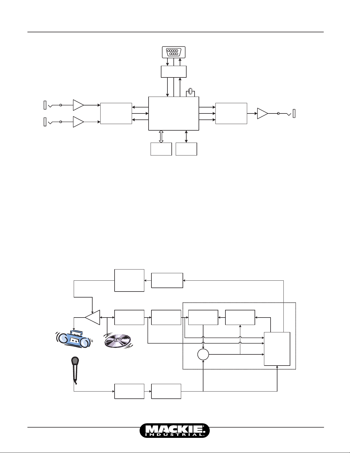
[8]. Figure 0 shows the hardware block diagram of the noise
sensor. The software is actually twofold: an embedded software algorithm plus application software (SP-Control™ for
the Palm™) to allow for ease of user control. Additionally,
the SP-DSP1™ algorithm allows for a high level of automation,
which in-turn, makes this system extremely easy to setup
and use. Unlike some of the earlier attempts at “noise sensing”,
the SP-Control™ software requires no complex procedures
during setup and calibration. The user simply places his speaker(s)
as needed and positions the ambient microphone so that it is
listening to the primary noise source. Then the appropriate
gain structure is setup as well as a few room-specic user
parameters. Finally, while playing music, an Auto Calibration
is initiated. It’s fast and simple!
September 2000
1
Page 2
Mackie Industrial White Paper Noise Sensing
32-bit
Floating-Point
DSP
Stereo
DAC
Stereo
ADC
EPROM
SERIAL
EEPROM
Program Input
Ambient Mic
Input
Program
Output
RX
GND
`
TX
RS-232
TRANS.
RS-232 DSUB9
FIR
Down
Sampler
Down
Sampler
Anti-Alias
Filter
Anti-Alias
Filter
G
RMS
Measure
Coefficient
Calculator
Compander
error
Y
-
+
Noise
Threshold
Override
nLMS Adaptive Filter
Figure 0: Hardware Block Diagram
1 Algorithm Overview
This section summarizes the Ambient Noise Sensing Algorithm
(see Figure 1) implemented in the SP-DSP1™. The algorithm is
used to increase the sensitivity to ambient noise in the room by
rejecting the source signal (music) that is broadcast into the room.
This allows the SP-DSP1™ to control the volume of the music
based on the room ambient noise. The better the rejection of the
music signal the more sensitive the gain control without runaway
gain problems.
The algorithm adapts to the room characteristics by comparing
the room response to the source signal. It computes its own
approximation of the room response in order to cancel the music
signal from the signal picked up by a room microphone [1-5,7].
Room size is the most important factor determining the effectiveness of the algorithm. Small rooms (ofce size) can achieve as
much as 40dB music rejection, while larger rooms (nightclubs
or restaurants) might only achieve 10-20dB. Even 10dB rejection
allows noticeably better sensitivity to noise.
2
Figure 1: Algorithm Block Diagram
September 2000
Page 3

Mackie Industrial White Paper Noise Sensing
1.1 Algorithm Block Diagram
The ambient noise sensor algorithm is a variation of a Normalized LMS Adaptive Filter [2-4, 7, 11-12]. The coefcient
calculator in the system uses the error signal, some Root Mean
Square (RMS) signal levels and energies, and the current coefcients to compute a new set of Finite Impulse Response (FIR)
coefcients that approach the Room Transfer Function (RTF) [5].
Down sampling has been used to optimize the adaptation characteristics of the algorithm for the largest room possible using
minimum MIPS and memory [8, 9]. The compander controls the
gain of the music signal based on the ambient noise detected and
the user input parameters.
1.2 Normalized LMS Adaptive Filter
The Normalized Least Mean Square (nLMS) Adaptive Filter
portion of the Ambient Noise Sensor consists of the FIR lter
(Equation 1), Coefcient Calculator (Equation 2), Summation
(producing the error signal), and RMS measurements, and can
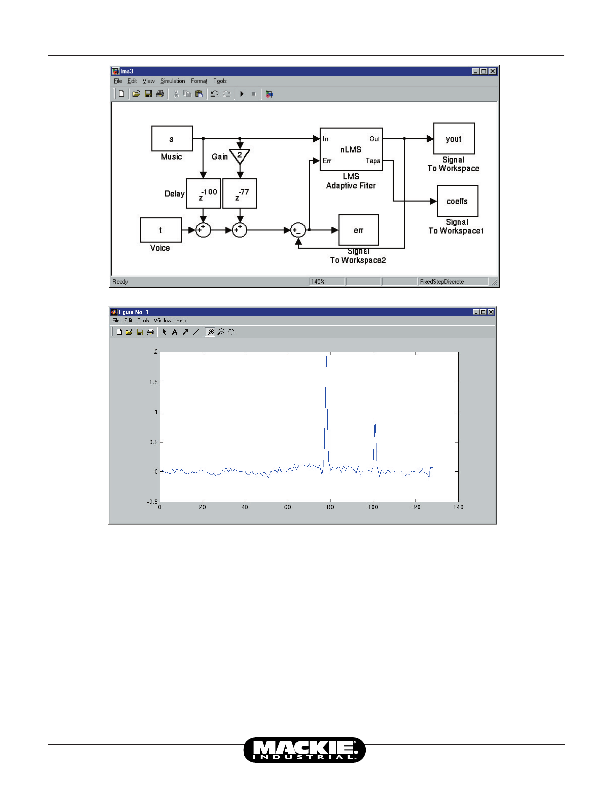
be considered equivalent to the MATLAB1 simulation shown
in Diagram 1 [1, 9, 10]. In this simulation the ‘Voice’ signal
is the ambient noise signal, the delays represent the RTF, and
the nLMS lter adapts to produce the ‘Out’ signal which
is an approximation of the music combined with the RTF.
When the output signal from the nLMS is subtracted from the
input signal (Voice + RTF (Music)) the ‘err’ or error signal
approximates the original ‘Voice’ or noise signal. Look at
the gains and delays shown in the blocks of Diagram 1 (simulating the direct sound plus one reection). The amplitude
versus time plot was generated with the coefcients from the
‘Taps’ output of nLMS lter. As you can see from this simple
example, this lter is the RTF. Obviously, in the real world,
the exact RTF is not obtainable. However, the better the
FIR approximates the RTF, the closer the error signal is
to the actual noise in the room [2-4, 11-12]. The nLMS Adaptive Filter is constantly adapting to the room characteristics.
This provides optimum performance when the room acoustics
change. Room acoustics can change signicantly due to the
arrangement of furnishings, opening or closing drapes, the
number of people in the room changing, or more dramatic
changes such as moveable walls or room dividers.
The effectiveness of the nLMS is determined mostly by the
number of taps in the FIR (internal to the nLMS adaptive
Filter), the adaptation algorithm, and the density and duration
of the RTF. In the SP-DSP1™ the processing capability and
memory allocation has limited the FIR length to about 1500
taps. As a result, the signals are down sampled to allow for
good cancellation even in reasonably large rooms. Since the
1
MATLAB is the trademark of a comercial matrix-based processing
language.
speed of sound is approximately 1 ft/ms, we designed the
system to provide adequate rejection for music paths (direct
sound plus reections) up to about 300 feet.
A standard Transversal n-point FIR lter was used [1, 5, 8].
Input buffering is n points long plus a little extra buffer space.
The Output, y, forms another buffer:
N-1
y(n) = ∑ w
(n)*u(n-i)
i
i=0
(1)
where
N = number of FIR taps or the order of the lter
n = time index
y = FIR output
w = adaptation coefcients
u = FIR input
Calculation of new coefcients (coefcient calculator) is
performed if the following two conditions are met:
• If the normalization energy is greater than zero (if
negative or 0 it is a debug error condition).
• If the Error Threshold signal is above the threshold
computed as a portion of the normalization energy of the
input signal.
Mathematical calculations for coefcient updating are
according to a slightly modied nLMS formula [2-4, 7,
11-12]:
Wi(n+1) = Wi(n)+ ————————
e(n) * beta * u(n-i)
epsilon * E(n)
(2)
where
n = time index
i = 0..n-1
W = FIR lter coefcients
e = error
u = FIR input data
E = Normalization Energy
beta = adaptation rate (function)
epsilon = stability coefcient
Our slightly different use of beta (not shown) plus the use
of an Error Threshold are unique adaptations of the standard
nLMS algorithm. The new beta function allows faster adaptation when the error, e, gets smaller. The normal use of beta
as a scaling value (shown above) requires a small value to
guarantee stability of the algorithm when the error is large,
September 2000
3
Page 4
Mackie Industrial White Paper Noise Sensing
Diagram 1: Matlab simulation Block Diagram and Results
which signicantly reduced the adaptation amount when the
error was small, extending the adaptation time to well over 30
minutes. Our beta function (patent pending) gives stability to
the algorithm when the error is large, but effectively shortens
the adaptation time dramatically when the error becomes
small. This allows the algorithm to adapt to a room in only
a few minutes.
For small rooms a signicant portion of the music energy due
to the paths from speaker to microphone (including reections) are removed by the nLMS algorithm, as there would
4
have to be many reections before the sound could have traveled this far. Each reection reduces the energy of the music
signal, and the amount of reduction of the energy is related
to the shape and material of the reecting surface. The more
‘live’ the room, the longer and more dense the RTF is, the
less the energy of the music signal that can be removed by the
nLMS lter [6]. Even without a lot of reections a very large
room may have poor cancellation due to the small number of
reections before the music signal has traveled the maximum
‘distance’ of the FIR.
September 2000
Page 5

Mackie Industrial White Paper Noise Sensing
1.3 RMS Measurements
The nLMS algorithm requires normalized energies for calculating the FIR coefcients. A real RMS algorithm is used to
measure the signal levels [2, 4, 11-12]. This is accomplished by
buffering the squares of each sample of the input signal (Square),
averaging the sum of these squares every sample (Mean), and
taking the square root of the mean (Root). For every input sample
an RMS value is produced, which is itself buffered and ltered
by a 256-point window function, to smooth the response of the
detector by a xed known delay and amplitude.
The main benet of ltered RMS measurement is to reduce
the impact of low frequency room energy variations caused by
the music broadcast into the room, which can give variations
in the room energy readings by 2 or 3 dB. This amount of
variation could cause the compander to constantly turn the
volume of the music up and down by a similar amount, which
is quite noticeable and undesirable.
Several RMS detectors are required in the system. The nLMS
Coefcient Calculator requires the energy of the FIR output,
error and music signals. The Compander requires the level of
the music and microphone signals.
1.4 Down Sampling
To extend the effective FIR length for larger rooms the LMS
lter is down sampled from the converter sample rate [8,9]. In
this implementation, 44100 Hz (Fs) is the converter sample rate
for the music and microphone signals. Down sampling also helps
reduce the memory and MIPS requirement. This also has the
effect of comparing energies of signals ltered at half of the
down sampled Nyquist rate. As long as the noise signal has a
proportional amount of its energy in this spectrum, the ambient
noise sensor will approximate the level of the noise signal. As we
have found, this is a valid assumption.
1.5 Compander
User parameters control the operation of the compander.
Minimum Gain, Gain Range, Noise Threshold, Noise Range,
Attack/Release Times, and RMS measurement parameters
determine how much gain (or attenuation) is applied to the
music signal.
The compander Attack and Release parameters control the
rate at which the gain is turned up or down. These are important to control the gain during loud sudden events such as door
slams, yells, or dropped dish trays, which would normally
cause the music level to be turned up very loud. A slow attack
rate (more than 10 seconds) with a faster release rate will
reduce the level of gain applied to the music. This allows the
compander to track the ambient room noise while ‘rejecting’
these singular events if desired.
1.6 Auto-Calibration
The biggest single problem with controlling the music gain based
on the room noise is runaway gain. Runaway gain occurs when
the compander turns up the music volume which is measured
as ‘room noise’, which tells the compander to further increase
the music volume. The compander must have the appropriate
information to prevent this cycle from occuring.
A calibrated algorithm for computing the approximate location at which runaway gain might occur is used as an override
to limit the sensitivity to the room noise. Although the algorithm constantly adapts to the room acoustics it takes a
signicant amount of time for the algorithm to get to its best
approximation of the RTF. Until this point is reached it is
not possible to determine the override conditions required to
prevent runaway gain. This condition would occur every time
the unit was reset (power on/off) were it not for the Auto
Calibration process, and the internal non-volatile storage of
the calibration parameters.
The Auto Calibration uses a real music signal with xed gain
to adapt and monitor the ambient room noise. As long as the
algorithm is making progress towards the RTF it will continue
to adapt and monitor the noise level. During calibration it
is best to have a minimum amount of room noise so that
the algorithm can determine the progress towards the RTF.
Once the progress towards the RTF has slowed signicantly
the current adaptation coefcients are stored and the Noise
Threshold Override is computed. Every time the unit is reset
the calibration coefcients and Noise Threshold Override are
restored. This allows the compander to prevent runaway gain
on reset and during normal operation. The algorithm continues to adapt at all times to keep up with room acoustic
changes, and as long as the room acoustics do not change
drastically the gain should be prevented from running away.
2 Hardware Setup
The SP-DSP1™ was designed to be an expansion card that is
added to our new “SP” or Sound Palette® series mixer/ampliers
(SP2400/1200). These ampliers provide one or two zones of
200 watts per channel in a two-rack-space package. Since the
SP-DSP1™ operates only on a mono program signal, one card
is required per channel. Once the card is installed, the user
needs to connect an ambient microphone to the rear panel of
SP2400/1200. Note that the connection requires a 3.08mm 3-pin
male Phoenix connector (i.e. Euroblock).
September 2000
5
Page 6

Mackie Industrial White Paper Noise Sensing
2.1 Ambient Microphone
Mackie Designs recommends the Mackie Industrial
MT3100® omnidirectional Electret microphone. This is an
excellent multi-standard phantom condenser microphone perfectly suited for noise sensing applications. However, for
many applications, any inexpensive low-impedance, omnidirectional microphone will sufce. An installer may nd that
a directional microphone is better suited for installations in
smaller or noisier rooms. The microphone should be placed
where it can “hear” the ambient noise within the room. This
(direct vibrations) from speaker to microphone should be
avoided as well as placing the microphone away from the
speakers to provide the best noise-to-signal ratio.
3 Palm™ Control
Mackie Designs has designed the SP-DSP1™ to run under the
Palm™ OS or any compatible palmtop device. The SP-Control™ Palm™ application (on 3 1/2 inch disk) is included with
the SP-DSP1™ hardware card and can be downloaded from
our WEB site at www.mackieindustrial.com. All necessary
cabling is provided to install the card into the SP2400/1200.
Additionally, a 3-inch null-modem adapter cable is provided
to connect a standard Palm™ Cradle or the HotSync® Cable
to the 9-pin female D-Sub on the front of the SP2400/1200.
After installing the application to your device, to run the SPControl™ software, simply select the “SP-Control” from the
available applications. You should see the main SP-Control™
window (see Figure 2). The main display has six user parameters and four bar graphs indicating the relevant levels. Because
of limited screen space, we used two-letter symbols designating the parameters and levels. Table 1 summarizes the six
parameter ranges and their default settings after a Factory
Restore.
Figure 2 SP-Control™ Main Screen
does not imply that the SP-DSP1™ can not differentiate
between the noise and the program material. However, to
get the best possible performance and rejection, the ambient
microphone should be placed where it is listening to the
“intended” ambient noise source. Any mechanical feedback
“MG”= “GR”= “NT”= “NR”= Attack/
Min. Gain Gain Range Noise Noise Range Release
(dB) (dB) Threshold (dB) (dB) Time (sec.)
Minimum: -40 0 -80 1 1
Maximum: 0 40 0 60 300
Default: -40 40 -40 40 1
3.1 User Parameters (Sliders)
As the parameter Minimum Gain implies, this is the lowest
level to which the system can attenuate. With this slider
default at –40dB, the system can attenuate the program input
by as much as 40dB. Please note that the SP-DSP1™ can
only attenuate program material that is present on the input.
That is, this system (see Figure 0) will never allow gain from
input to output (≤ 0dB). By setting the Minimum Gain and the
second parameter, Gain Range, you are actually establishing
the program operating window within which the levels for
the program material must remain. For example, if the user
wanted his music levels to operate in a range ±10dB around
-15dB down from the input level, he would set MG =-25dB
and GR=20.
Table 1: SP-Control™ User Parameter Ranges and Defaults
6
September 2000
Page 7

Mackie Industrial White Paper Noise Sensing
+10dB
+5dB
0dB
-5dB
-10dB
-15dB
-20dB
-25dB
-30dB
-40dB
-35dB
-50dB
-45dB
-55dB
-60dB
-65dB
-70dB
-75dB
-80dB
Default setting
Ratio: 1:1
Note: Ratio=Noise:Program
NT=-80
MG=-30
NR
GR
=Program Operating Window
=Noise Window
Unity:
FS:
GR NR
NT=-40MG=-40
Lowest NT, Highest NR
Ratio: 2:1
Sensitive to low noise
GR
NR
NT=-30
MG=-20
GR
NR
NT=-60
MG=-35
Average setting
Ratio: 3:2
Good for small room
Average setting
Ratio: 2:3
More Sens., Larger room
Good starting point
The second parameter, Gain Range, also sets the maximum
gain attainable from the Minimum Gain. That is:
Prog. Operating Window = Min. Gain + Gain Range = Max. Gain
(3)
The Gain Range slider “re-scales” so that system gain (input
to output) is never greater than 0dB. So, if MG =-10dB, then
GR≤10dB. In most cases, the user can ignore the Gain Range
parameter. He would simply set the desired Minimum Gain of
the music (either by listening or from calculation) and leave
the Gain Range at the default “re-scaled” setting.
The third parameter, Noise Threshold, sets the noise “trigger”
of the algorithm. Until the noise level exceeds this threshold,
the throughput program level is unaffected. This slider actually sets the “noise” sensitivity of the algorithm. NT is relative
to the unity point which is –10dBFs (from full scale). Therefore, if NT=-80dB, this would indicate a noise threshold level
of –90dBFs (where Fs = 1V RMS). In simplistic terms, the
lower the Noise Threshold (more negative), the more sensitive
program level changes are to noise level variations. The Noise
Threshold parameter in conjunction with the fourth parameter, Noise Range, actually sets the operating window of the
noise source. This noise “window” sets the level and range
that the noise must be within to effect the program level:
Noise Window = Noise Threshold + Noise Range (4)
The Noise Range setting gives the user control over how much
noise level change causes the program level to span it’s Gain
Range. By setting a small Noise Range (say 20dB) with regard
to the Gain Range (say 30dB), you are allowing a 20dB noise
level change to cause the program output level to span 30dB.
This is assuming that the noise level has crossed the Noise
Threshold. In other words, these settings would represent a
2:3 noise level to program level change (see Chart 1). For
every 2dB change in noise level, the output level changes by
3dB. On the other hand, NR=40 and GR=40 (default settings)
September 2000
Chart 1: Noise Window vs. Program Operating Window Examples
7
Page 8

Mackie Industrial White Paper Noise Sensing
would represent a 1:1 noise level versus program level change.
You can start to see the exibility of this system (see Chart 1).
By having control over the program operating window (MG
and GR) and the noise window (NT and NR), the user can
actually move the noise window with respect to the program
operating window and visa versa. In this way, the system can
be set to be “sensitive” to small noise changes or “insensitive”
to large noise changes and everything in between.
3.2 Attack and Release Parameters
The Attack parameter denes the time, in seconds, it takes for
the Program Gain to increase by 40dB. Likewise, the Release
parameter denes the time it takes for the Program Gain to
decrease by 40dB. The combination of these two parameters
gives the user the ability to “average” the noise to provide
a relatively constant Program Gain over time. Otherwise,
with short attack and release times (i.e. the default settings),
the user will hear every program level shift as it relates to
a specic noise level shift. To keep impulsive noise bursts
from affecting the program level, a good setting would be
an Attack =20 seconds and Release =20 seconds. This would
avoid the impulsive change but would still allow a fairly
“responsive” program level change as it relates to a noise
level change (~40 seconds). In a plant setting where there are
numerous pages and “break time” buzzers, setting the Attack
and Release Time on the order of minutes, will eliminate
program level changes on all but the average long-term noise
level. There may be a situation where you want a long Attack
and a short Release Time or visa versa. For example: in a plant
with background music, equipment may be turned on sequentially (relatively slowly) in the morning but in the evening
all are switched off together. A long Attack but short Release
Time might be advantageous by allowing the music level to
decrease instantly when the noise level fades.
is executed, ensure that the microphone level is within the
range from 0 to –10dB for the loudest noise plus program
expected. On the rear panel of the SP2400/1200 ampliers,
there is an “ambient mic” trim potentiometer. Adjust this trim
potentiometer (0-55dB) to get the proper levels as indicated by
the “MI” meter. Note that the SP-DSP1™ does not have a mic
preamp. Therefore, it is essential that the ambient microphone
input receives a line-level signal (1 V RMS Full-scale). The
third meter from the left as shown on the SP-Control™ screen
is the “PG” meter which is the Program Gain. This meter
represents the gain (0 to 60dB) that algorithm applies to
the Program Input. The last meter is the “PO” which is the
Program Output meter. This is the level at the output of the
SP-DSP1™ (0 to 60dB). The following condition will always
be true:
Prog. Output level = Prog. Input level + Prog. Gain (in dB) (5)
A good way to set the proper “MI” level is to select the Bypass
button on the main screen. Then, while playing typical program
material, adjust the microphone preamp trim potentiometer on
the rear panel of the SP2400/1200 until the “MI” meter is within
0 to –10dB. This allows us to adjust the level while the microphone is “hearing” both the program material plus the noise so
that we do not inadvertently clip the SP-DSP1™ microphone
input during calibration. Clipping the microphone or program
input (ADC) will produce erratic controller behavior and should
be avoided.
3.3 Bar Graphs/Metering
The main screen of the SP-Control™ Palm™ application has
four meters that allow the user to monitor levels during setup
and normal operation (see Figure 2). “PI” is the Program
Input meter and it indicates the input level into the DSP (range
from 0 to 60dB). During setup before Auto Calibration, the
user needs to ensure that the input program source has sufcient signal level by monitoring this meter. The input level
should be between 0 and –10dB during the loudest portions
of the program material. “MI ” is the Microphone Input meter.
This meter indicates the ambient microphone input level in
a range from 0 to 60dB. Again, before an Auto Calibration
8
Figure 3: SP-Control™ Save Conrmation
September 2000
Page 9

Mackie Industrial White Paper Noise Sensing
3.4 Additional Main Screen Options
The main screen of the SP-Control™ also provides the ability
to save and recall 10 presets. These presets are stored in the
EEPROM onboard the SP-DSP1™ (see Figure 3). A preset
consists of the following parameters: Minimum Gain, Gain
Range, Noise Threshold, Noise Range, Attack and Release
Times. There are two Global parameters that are recalled at
power up and displayed when Connect is selected on the main
screen. These include the Bypass state and the CAL or calibration value. Additionally, the preset that was saved or recalled
when the SP-Control™ was last connected will be stored in
the EEPROM and recalled at power up. The CAL value is set
during Auto Calibration and will be discussed in the next section. The Bypass toggle, as its name implies, allows the user
to bypass program input to program output and effectively
disables the algorithm. This is a useful feature during setup
to ensure the proper levels are obtained. Finally, the DSP1/2
toggle allows the user to change between communicating with
DSP1 or DSP2. As you are already aware, the SP2400/1200
can support two SP-DSP1™ cards; one for each zone. Therefore, if your system has two controllers, this toggle allows you
to control each card separately and independently.
tion to ensure that all levels are in their target range as
suggested in Section 3.3 Bar Graphs/Metering. If you nd that
the microphone and input levels are too low or too high, you
may want to Abort the calibration by selecting the appropriate
button and then readjust the levels accordingly. There is also
an End & Save button if the user nds that calibration is
3.5 Auto Calibration
The Drop Menu of the SP-Control™ has several functions
shown in Figure 4. The Auto Calibration provides the user
with the ability to automatically adapt his speaker-microphone
placement to the room acoustics (patent pending). This function eliminates the tedious calibration procedures associated
with other competitor’s products. Additionally, the possibility
of “runaway” system gain is greatly reduced because the algorithm (a modied nLMS adaptive lter) is constantly making
“running” changes to obtain the best noise-to-signal ratio.
To maximize the results, an Auto Calibration should be performed while the room noise is at a minimum. However, since
the algorithm adapts over time, this is not a critical requirement. Once the speaker(s) and ambient microphone are in
their xed locations and the microphone gain and input levels
have been adjusted (per Section 3.3 Bar Graphs/Metering),
simply select Auto Calibration while playing standard program material. Prior to performing the Auto Calibration,
please ensure that the front panel level control on the
SP2400/1200 is set to the maximum sound level that you
would ever expect the system to deliver. Recall that the noise
sensor only attenuates the signal from input to output. During
the calibration, a count-down timer is initiated at 90 seconds
and a progress meter is displayed. If the algorithm nds that
adaptation improvements are possible, the timer is reset to
90 seconds. A typical calibration period is 2-3 minutes. It is
advised to monitor the main four meter levels during calibra-
Figure 4: SP-Control™ Function
taking too long or music breaks are causing count-down timer
resets. Typically, music breaks between songs are no problem.
However, if the break is too long, the calibration may be
ineffective resulting in numerous timer resets. If this becomes
a problem, simply changing to different program material
or using music with shorter pauses between songs should correct the situation. Once the calibration is complete, the CAL
value will update. At default, this value is +10 (range: +20
to –80dBr). This number is a measure of how much of the
program material is getting rejected in the environment that
the Auto Calibration was performed. The closer the number
is to +10, the less rejection. A CAL = -15dBr would be an
excellent rejection and would be expected in a small room.
However, in larger rooms and auditoriums, the rejection will
be less (closer to 0dBr). Remember that this number is only
an estimate of rejection that is used by the algorithm to set the
Noise Threshold Override.
September 2000
9
Page 10

Mackie Industrial White Paper Noise Sensing
3.6 Factory Restore
If you nd that the EEPROM is corrupted or has not been initialized from the factory, you can perform a Factory Restore
upon installing the SP-DSP1™ and running the SP-Control™
application. A new SP-DSP© card should have all parameters
of all presets set to default values (see Table 1).
3.7 Upload/Download From/To EEPROM
Occasionally, it is necessary to backup SP-DSP1™ presets and
parameters or to transfer settings from one DSP to another.
To copy the contents of the EEPROM, simply Connect to
the DSP card and then select Upload From EEPROM. The
EEPROM contents are stored in your Palm™. If you would
like to copy contents of the Palm™ into another SP-DSP1™
card, select the Download To EEPROM. Be advised that this
will completely erase the existing contents of the EEPROM
and replace with what was uploaded to the Palm™. Be careful
to do an Upload From EEPROM before the Download To
EEPROM to ensure that valid data exists in the Palm™.
4 Tips for Setting User Parameters
To clarify, setting the user parameters (MG, GR, NT, NR,
Attack Time and Release Time) can be done either before or
after the Auto Calibration. These parameters have no bearing
on the calibration and can be changed at any point. In fact, a
Preset Save and Recall only affect these parameters.
The Auto Calibration only concerns itself with the Calibration
or CAL value and the adaptation coefcients. The user parameters can be set up for runaway gain, but the user would
notice this immediately as the system would “runaway” to
the maximum gain. During calibration, the user parameters
are temporarily overridden to perform the calibration at a
xed gain (easier and better results). However, the xed gain
used during the calibration process is the Maximum Gain
(Minimum Gain + Gain Range). It is probably advisable for
the user to set up these two parameters so that he isn’t “blown
away” by the calibration sequence if his Maximum Gain is
louder than he intends. The Maximum Gain is used as the
calibration value because the algorithm adapts more quickly
when the music is loud. The calibration itself doesn’t limit
the parameters the user can adjust in any way, it just provides
a ‘hidden override’ when he has his Noise Threshold set too
sensitive, which would otherwise cause runaway. You’ll notice
that once your unit has been calibrated you can set the Noise
Threshold as low as you want and you will still seem to get
the same sensitivity. This is because it is being limited by the
Noise Threshold Override (see Figure 1).
As you can see, one of the rst questions that the end-user
needs to answer is “How much overall system gain or attenuation do you want the noise sensor to provide?” By answering
this question you have determined the setting of the Gain
Range (GR). A typical good starting point for the Gain
Range is about 20dB. If you nd the system does not attenu-
ate enough or attenuates too much, adjust accordingly. By
answering this rst question, you are likely to determine the
Minimum Gain (MG) as well. Since the average user would
want his system to attenuate from the unity point (0dB),
which is the highest sound level he would ever want, for
this example the Minimum Gain would be set to –20dB. As
mentioned in Section 3.1 User Parameters (Sliders), by setting
the Minimum Gain and the second parameter, Gain Range,
you are actually establishing the program operating window
within which the levels for the program material must remain.
As in the previous example, if the user wanted his music levels
to operate in a range ±10dB around -10dB down from the
input level (unity point), he would set MG=-20dB and GR=20.
Setting the Noise Threshold (NT) can only be done by determining the noise level at which you want the music to start
to increase in level. This noise threshold point is best found
through trial and error. You must be careful not to set the
NT too low (i.e. more negative), because the noise sensor will
begin “gaining up” the program material with very little noise.
However, setting the NT too high will prevent the system from
making any program gain increases until there is a relatively
high noise level. There is a balance and each room will require
a different NT setting. Keep in mind that setting this level in
an empty room may require some “tweaks” when the room
is full with people. For example, if you set NT=-40dB in an
empty restaurant, you may nd that the system starts gaining
up too fast and is too loud for the occasion. In this case, you
can reduce NT (by bringing the level closer to 0dB) by 5 to
10dB. This would give you NT=-30 to -35dB and the system
would not start “gaining up” until the noise was 10dB “hotter”
than it was previously.
Noise Range (NR) actually sets the amount of noise that makes
the program gain go from the minimum setting to the maximum setting. That is, if NR=40dB and GR=20dB, then for
every 2dB change in the Noise, the Program level is only
10
September 2000
Page 11

Mackie Industrial White Paper Noise Sensing
changed by 1dB. A good starting point is to set NR equal to
the GR setting. This would give a 1:1 noise to program level
change and would sufce for the majority of installations.
Remember, The Noise Threshold Override will protect the
system from runaway gain even if the NT and NR are set
incorrectly
5 What to Avoid
Once an Auto Calibration has been performed, a user should
never move or change the speaker-microphone placements. In
fact, any changes (i.e. adding more speakers, moving equipment, signicantly changing the room layout, etc.) should
be avoided. If these changes are required, simply recalibrate
by initiating another Auto Calibration. You may nd that in
environments that change daily (new equipment added, equipment moves, etc.) a periodic recalibration would be benecial.
Any gain adjustments made to the microphone preamp should
be done prior to Auto Calibration. Further-more, all level
changes should be made prior to the DSP card. If the system
gain is changed in any way post DSP card, the noise sensor
perceives this as an acoustic noise disturbance. This is why
the level controls on the SP2400/1200 are before the DSP.
Again, any level changes made after the DSP card (i.e. power
amplier, speakers, between the preamp and power amplier,
etc.) will require a recalibration.
6 HyperTerminal Control of SP-DSP1™
If the user does not own a Palm™ or compatible device, he
can use HyperTerminal available on any PC running Windows
OS. HyperTerminal can control all the parameters previously
mentioned. The null-modem adapter is not necessary as the
9-pin female D-Sub on the front of the SP2400/1200 will
connect directly to a PC COMM Port. Mackie Designs will
provide a one-page protocol at the customer’s request.
8 References
[1] Antoniou, A., 1993, Digital Filters: Analysis, Design, and
Applications, 2nd ed., McGraw Hill.
[2] Cowen, C. F. N. and P. M. Grant, 1985, Adaptive Filters,
Englewood Cliffs, NJ: Prentice Hall.
[3] Franklin G. F. and J. D. Powell, 1981, Digital Control of
Dynamic Systems, Reading MA: Addison-Wesley.
[4] Haykin, S., 1986, Adaptive Filter Theory, Englewood
Cliffs, NJ: Prentice Hall.
[5] Haykin, S., 1989, Modern Filters, New York: Macmillan.
[6] Hellman, Zwislocki, September 1964, “Loudness Function
of a 1000-cps Tone in the Presence of a Masking Noise”,
Journal of the Acoustical Society of America, v. 36, no. 9, pp.
1618-1627
[7] Morzingo R. A. and T. W. Miller, 1980, Introduction to
Adaptive Arrays, New York: Wiley.
[8] Proakis, J. G. and D.G. Manolakis, 1988, Introduction to
Digital Signal Processing, New York: Macmillan.
[9] Proakis, J. G., 1989, Digital Communications, Chapter 6,
McGraw Hill.
[10] Sondhi, M. M. and D. A. Berkley, August 1980, “Silencing echoes on the telephone network”, Proceedings of the
IEEE, v. 68, no. 8, pp. 948-963.
[11] Treichler, C. R., J. R. Johnson, and M. G. Larimore, 1987,
Theory and Design of Adaptive Filters, New York: Wiley.
[12] Widrow, B. and S. D. Stearns, 1985, Adaptive Signal
Processing, Englewood Cliffs, NJ: Prentice Hall.
7 Patent Protection
The basic principles of noise sensing presented in this paper
are the subject of patent applications.
September 2000
11
Page 12

Mackie Industrial White Paper: Noise Sensing 9/00
THE AUTHORS
Jeff Sondermeyer was born in
Denville, NJ, in 1963. He received his
B. S. in electrical engineering from
Mississippi State University, MS, in
1987 and his M. S. in electrical
engineering from the University of
Colorado, CO, in 1993. His thesis
research was conducted in speech
recognition where a Backpropagation
Neural Network was used to recognize stressed isolated words. During and after his graduate
work, he was a Digital Design Engineer for Peavey Electronics where he designed numerous audio effects processors to
include algorithms for pro audio gear. Presently, he is a Senior
Design Engineer/Digital Design Lead for Mackie Designs
where he has designed the low-cost EMAC multi-effects card
for the PPM and CFX mixers and the DX8; a two-rack 8x2
digital mixer. He is a member of the IEEE and AES.
Dale Shpak was born in Seattle,
WA, in 1957. He received his B. S. elec-
trical engineering from the University
of Calgary, Alta., in 1980 and his
M. S. in electrical engineering (elec-
tronics) from the University of Calgary,
Alta., in 1982. He received a Ph.D.
in electrical engineering from the
University of Victoria, B.C., in 1989.
Presently he is the Vice President of
Software Development with SysCor R&D Inc. He has done
research in digital lter design, signal processing for: audio,
speech, and telecommunications. Additionally he had done
work with networks to include networked Java applications. He
is the author of the DSP Blockset, Signal Processing Toolbox,
and a New Toolbox for Matlab/Simulink. He has numerous
publications in IEEE and one in AES (see: www.ece.uvic.ca/
~dale/cv.pdf). Dr. Shpak is a member of the IEEE.
Brian Roden was born in Ragina,
Sask. Canada, in 1963. He received a
Diploma of Technology in 1983 from
Camosun College, Victoria, Canada
and his Bachelor of Engineering from
University of Victoria, Victoria, B.C.,
Canada. He was previously employed
by IVL Technologies in algorithm
development and DSP implementa-
tion. He co-authored a patent on
Vocal Gender Shifting for IVL Technologies. In 1998, he was
the co-founder of Acuma Labs Inc. and is currently a Senior
Design Engineer.
Chris Jubien was born in Mon-
treal, Canada, in 1967. He received
his B. A. of Science from Waterloo
in 1990 and his M.A. of Science
from the University of Victoria,
B.C., Canada, in 1993. Previously he
work for IVL Technologies in algorithm development and audio effects
design. Presently he is the DSP man-
ager for Acuma Labs Inc. of which he
co-founded in 1998. His passion is real-time DSP algorithm
and effects development and has a strong interest in using
cutting edge technology to create new sounds and products.
Costa Lakoumentas comes from
Vancouver, British Columbia, where
he lived for 29 years. From 1981 until
1999, he owned two sound contracting businesses and represented nearly
all of the leaders in the pro-audio
industry. Joining Mackie Designs
Inc. in 1999, he was responsible
for the development and launch of
the company’s new Mackie Industrial
division. Mr Lakoumentas is currently Vice President of Business Development at Mackie Designs and is responsible for
all product concept and product development activities at the
Company.
12
 Loading...