

Page 1
MICROWAVES FOR EVERYONE
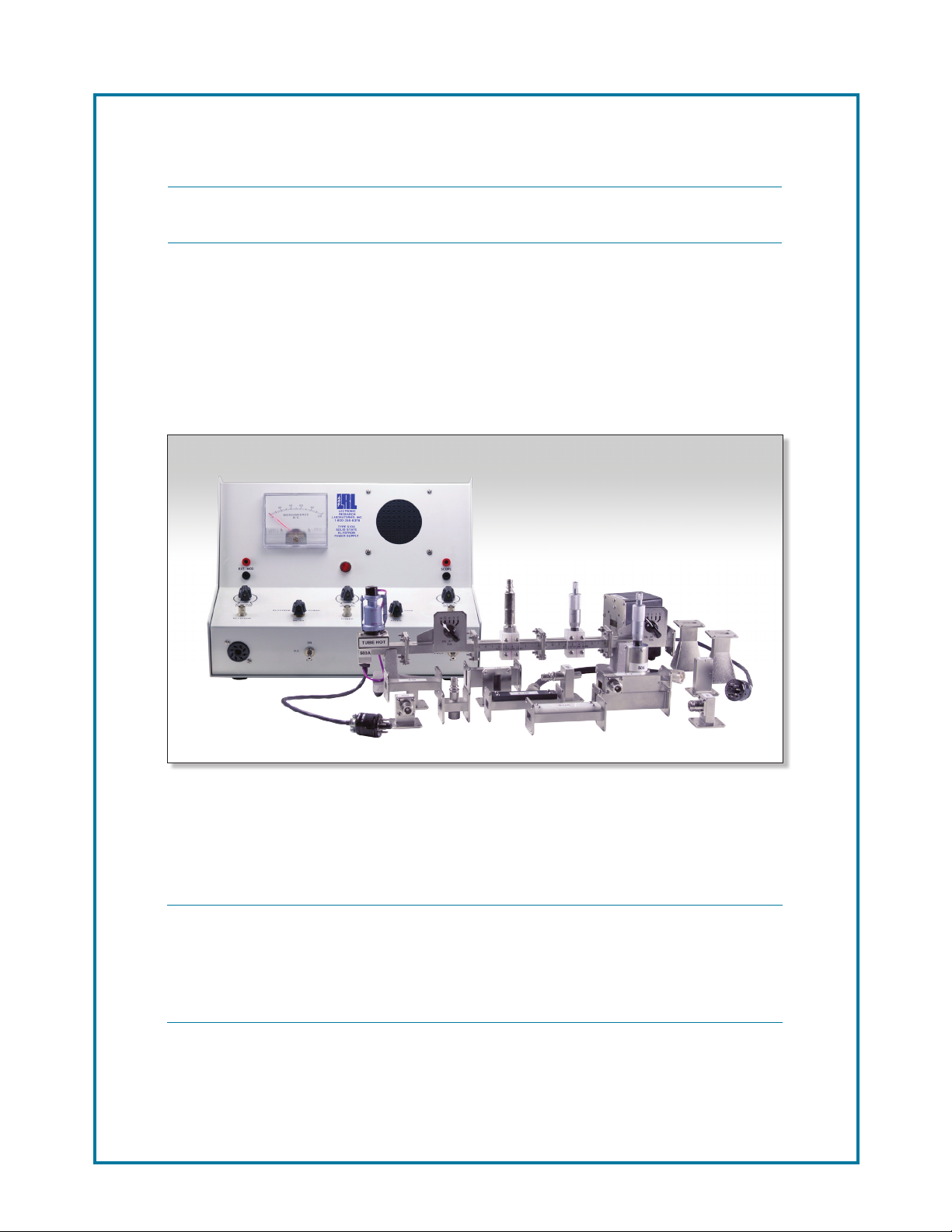
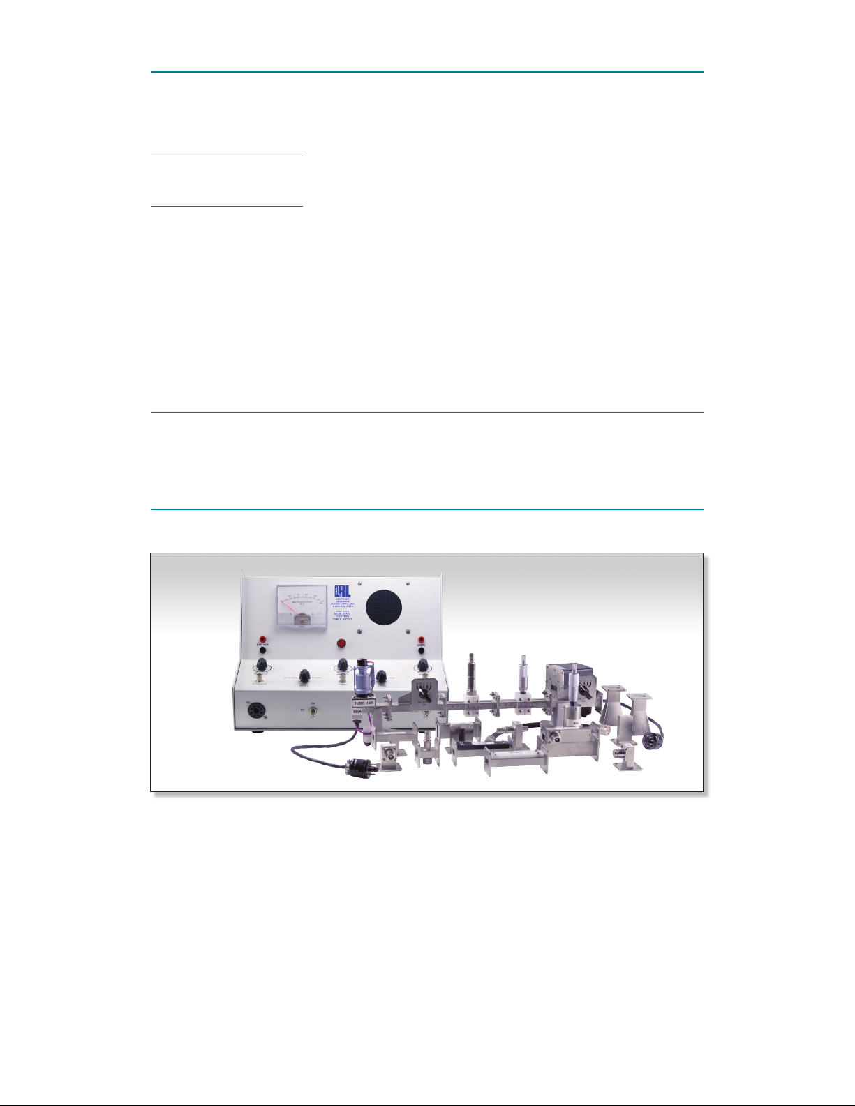
LRL Model 550B-SS
Microwave Training Kit
Microwave Training Kit
5 Experiments
I-95 Industrial Park
651 Winks Lane
Bensalem, PA 19020
800.523.3929 • 215.638.1100
3rd edition
Page 2

INITIAL SET-UP PROCEDURES • INVENTORY & SET-UP
COMPLETE PARTS LISTING
1 #503A with
2K25 Klystron
Tube Mount
1 #504 Frequency
Meter
1 #505 Slotted Line
1 #508 Thermistor
Mount
1 #518 Detector
Mount
4 #523
Waveguide
Stands
2
2 #506 Variable
Flap Attenuator
1 #507 Termination
Microwaves for Everyone | LRL 550B Microwave Training Kit
2 #531 Horn
Antennas
1 #532
Shorting Plate
Page 3
CONTENTS
Inventory & Set Up The LRL 550B Microwave Student Lab . . . . . . . . . . . . 4
Introduction A Brief Discussion of Transmission Line Theory . . . . . . . . 9
Experiment 1 Measurement of Power. . . . . . . . . . . . . . . . . . . . 15
Experiment 2 Measurement of Standing Wave Ratio . . . . . . . . . . . . 23
Experiment 3 Measurement of Frequency and Wavelength . . . . . . . . 31
Experiment 4 Propagation of Microwaves . . . . . . . . . . . . . . . . . 37
Experiment 5 Microwave Antennas . . . . . . . . . . . . . . . . . . . . . 43
LRL Model 550B-SS
X-Band Microwave Training Kit Frequency Range
X-Band 8.2-12.4 (GHZ)
The System Klystron is tuned to (9.3 GHZ)
Microwaves for Everyone | LRL 550B Microwave Training Kit
3
Page 4
INITIAL SET-UP PROCEDURES • INVENTORY & SET-UP
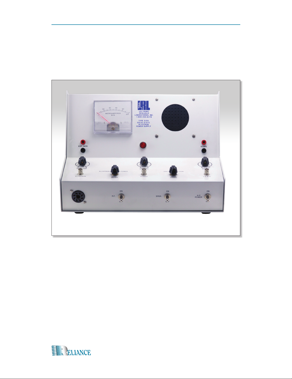
LRL 510A POWER SUPPLY
(thermistor bridge & amplifier)
4
Microwaves for Everyone | LRL 550B Microwave Training Kit
Page 5

PLEASE READ CAUTIONS CAREFULLY
BEFORE CONTINUING
CAUTION 1:
Klystrons get extremely hot when in use and must not
be handled while hot! Serious burns can result.
CAUTION 2:
Klystron mount, power supplies, and Klystron tube
plate caps have high voltages present when in use.
Exercise extreme CAUTION!
Shock or death can result.
CAUTION 3:
R-F power levels in this kit are not harmful, but a
human eye may be damaged by low levels of
radiation.
Do not look into any waveguide at any time when
units are on.
Microwaves for Everyone | LRL 550B Microwave Training Kit
5
Page 6

INITIAL SET-UP PROCEDURES • INVENTORY & SET-UP
INITIAL SET-UP PROCEDURES
The following steps will help you test your new 510A Solid State Power Supply to make
sure it is fully operational and ready for use. It also will give you the opportunity to
operate and become familiar with the entire system before attempting the experiments
listed in this manual.
Equipment & Components
• 510A Power Supply
• 503A Klystron Mount - with 2k25 Klystron installed.
• 506 Flap Attenuator
• 518 Crystal Detector
• 508 Thermistor Mount
• 515 24" BNC Cables (2)
• 523 Waveguide Stands (2)
Part 1 • Control Settings
Set switches and controls on 510A as follows:
1. AC Power Switch OFF
2. Speaker Switch ON
3. RF Switch ON
4. Attenuator Switch 0dB
5. Meter Switch POWER
6. VSWR Output Control MAX. COUNTER CLOCKWISE
7. Power Balance Control 12 O’CLOCK
8. Klystron Repeller Control 12 O’CLOCK
Part 2 • Waveguide Component Assembly Procedure
1. Connect 503A Klystron Tube Mount to left side of 506 Variable Flap Attenuator.
2. Connect right side of 506 Variable Flap Attenuator to left side of 518 Detector
Mount with the BNC Connector in the UP position.
3. Connect right side of 518 Detector Mount to the 508 Thermistor Mount with the
BNC Connector in the UP position.
4. Using BNC Cable, connect 518 Detector Mount to VSWR input connector located
on right side of 510A Power Supply.
6
5. Using second BNC Cable, connect 508 Thermistor Mount to POWER input
connector located at center of 510A Power Supply.
Microwaves for Everyone | LRL 550B Microwave Training Kit
Page 7

6. Insert 8-Prong Plug from 503A Klystron Mount into socket located on left side of
510A Power Supply.
7. Place a 523 Waveguide Stand under each side of Test Assembly, and adjust each
stand until the assembly is elevated in a stable position.
Part 3 • Operation and Checkout
1. Turn AC POWER switch ON.
2. Turn 506 Flap Attenuator to 24dB.
3. Observe meter and adjust POWER BALANCE knob to obtain a zero meter
reading. Turning knob clockwise increases meter reading; counter-clockwise
deceases reading.
4. Allow 3-5 minutes warm-up at this time.
5. Readjust POWER BALANCE knob to compensate for drift if necessary.
NOTE: The meter reading must be at zero to progress further.
6. Set Variable Flap Attenuator to 0dB.
7. Slowly turn KLYSTRON REPELLER knob clockwise and stop when you get a peak
reading on the meter. (Normally about 2 o’clock). NOTE: Adjust Variable Flap
Attenuator as needed to keep meter level between 70% and 100%.
8. Turn METER knob to VSWR position.
9. Fine tune KLYSTRON REPELLER knob as needed to obtain a stable, peak meter
reading. NOTE: This reading should be between 50% and 100% and must be stable. If not,
adjust VSWR OUTPUT knob on right side of 510A Power Supply.
10. Turn METER knob to KLYSTRON position.
11. Remove BNC Cable from VSWR Input Connector at right side of 510A Power
Supply and reconnect cable to KLYSTRON connector on left side of 510A Power
Supply.
12. Adjust Variable Flap Attenuator as needed to attain a peak meter reading. DO NOT
exceed a 100% reading on the meter.
13. Record meter reading and Variable Flap Attenuator level as your Klystron life
reading. NOTE: You can compare this reading to current readings anytime in the future to
determine the condition of the Klystron tube.
14. You have now successfully operated and checked out your Microwave Trainer. It is
important that you turn off the Trainer properly as described below.
Part 4 • Shut Down Procedure
1. Turn off AC POWER switch located on right side of 510A Power Supply.
2. Unplug 510A Power Supply from 115AC Power Source.
3. Wait for Klystron Tube to cool down (minimum of 10 minutes).
4. Disconnect all cables and disassemble waveguide components.
Microwaves for Everyone | LRL 550B Microwave Training Kit
7
Page 8
introdUCtion – Let’S tALK ABoUt trAnSMiSSion LineS
INTRODUCTION
Transmission lines come in a variety of physical types – coaxial, parallel conductors, and
waveguide are the most common. No matter which type we use, there are four elements
that inuence any physical transmission line:
A. Series inductance: L
B. Series resistance: R
C. Shunt or parallel capacitance: C
D. Shunt or parallel conductance: G
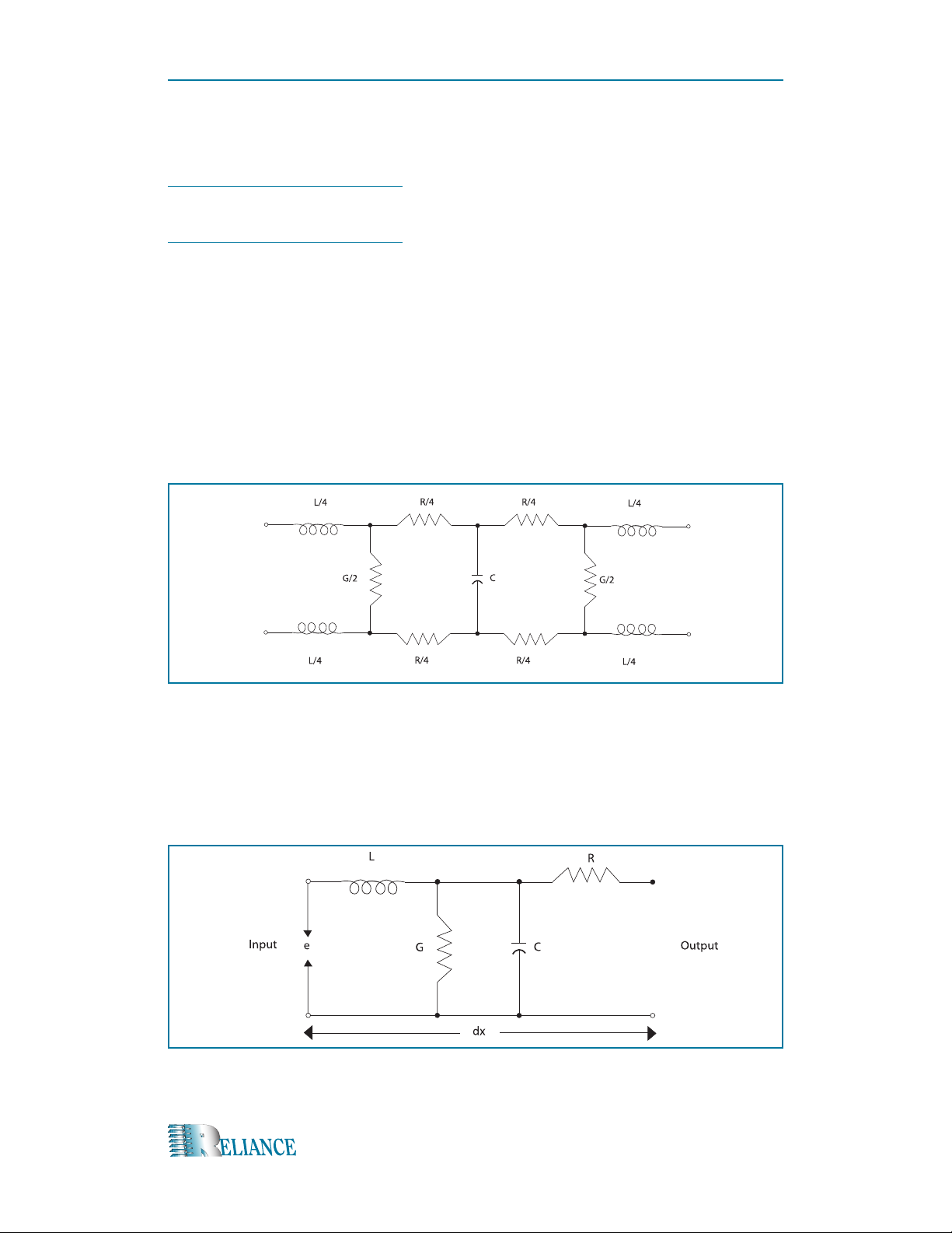
First, let us consider how a unit length of line is represented by Figure 1.1.
8
Figure 1.1 Unit Length of Transmission Line
The four different elements are represented by the fractional distribution along the entire
length of the line. If the line is to be satisfactory for practical use, it must remain
fractional proportional for any length – long or short. Once this principle is understood,
we can now use the simplied circuit diagram in Figure 1.2.
Figure 1.2 Simplied Unit Length of Transmission Line
Microwaves for Everyone | LRL 550B Microwave Training Kit
Page 9
The most widely used unit of measurement for transmission lines is the meter. This
should come as no surprise to you because wavelength and frequency have been
expressed through this unit of measure since the very start of microwave technology.
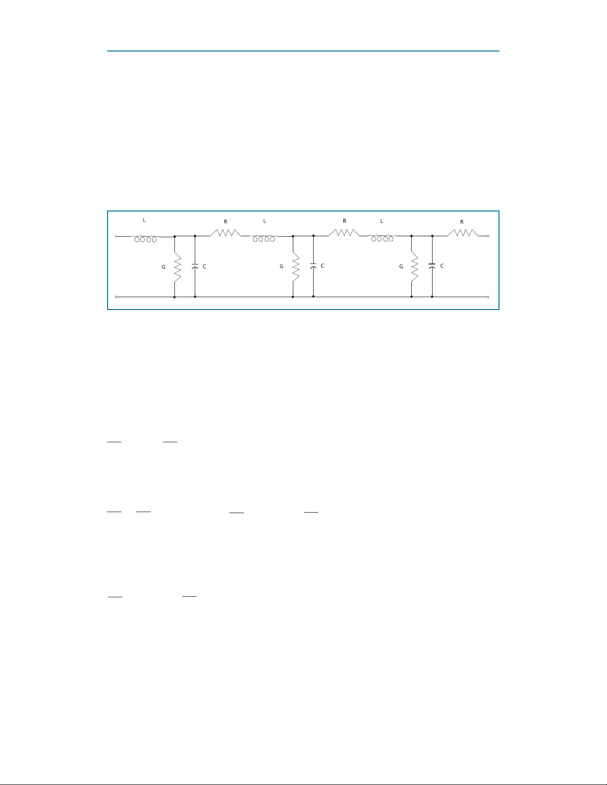
The expressions of L, R, C, and G are representative of one unit length of transmission
line dx. When unit lengths appear as two or more lengths, they can be seen as depicted
in Figure 1.3.
Figure 1.3 Several Unit Lengths of Transmission Line
However, the importance of fractional proportionality along any length of line may be
described simply as shown in Figure 1.2. If we apply a voltage e between the input
conductors shown in Figure 1.2 and the voltage varies at the rate de/dt, the shunt
current, di per unit length of dx equals the sum of the capacitive current and the
conductive current:
di
s
=EG+C
dx
Consequently, the shunt current represents the way in which the input current i is able to
change in a unit length dx Therefore:
di
+ = 0
dx
When the input voltage e is changing with time, the current will follow. This current
change can be shown as di/dt. The current change causes the series voltage to change
along dx and can be expressed as:
de
= - iR + L
dx
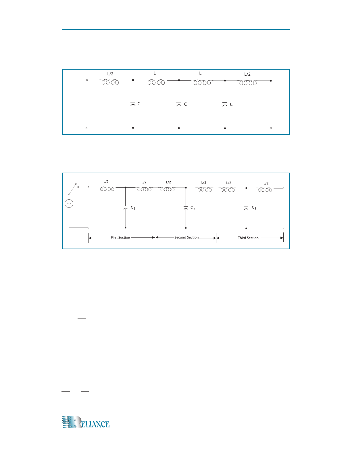
These equations are usually most helpful when a general approach (Fig. 1.1) to transmission lines is desired. However, with most applications, a general approach is not
necessary. In practical use, a short transmission line is utilized, and the line is said to be
“lossless” there by simplifying our analysis even further. The application circuit is shown
in Figure 1.4:
de
dt
di
s
dx
di
( )
dt
and
di
= - eG + C
dx
de
( )
dt
Microwaves for Everyone | LRL 550B Microwave Training Kit
9
Page 10
introdUCtion – Let’S tALK ABoUt trAnSMiSSion LineS
Figure 1.4 Lossless Transmission Line
In Figure 1.5, we will examine this line as a number of T sections connected together to
represent the line.
Figure 1.5 Sectioned Lossless Line
When we close “s1”, a signal travels through the line. The energy Q taken from the signal
source is: Q = it where t is the time of current ow. As the signal ows down the line, its
energy will be stored in the capacitors. So any single section is Q = Ce. If capacity C and
voltage e are shown, it follows that it = Ce. Once C1 has fully charged, C2 is still at zero
charge and the inductance L between them has a voltage equal to e. Therefore:
di
e = L
dt
Simplifying this relationship produces:
et = Li
If we divide:
et
Li
=
it
Ce
10
Microwaves for Everyone | LRL 550B Microwave Training Kit
Page 11
We end up with:
e
= √L/C
i
This last equation is most often referred to as “impedance” or ZO. Accordingly:
e
=Z0= √L/C
i
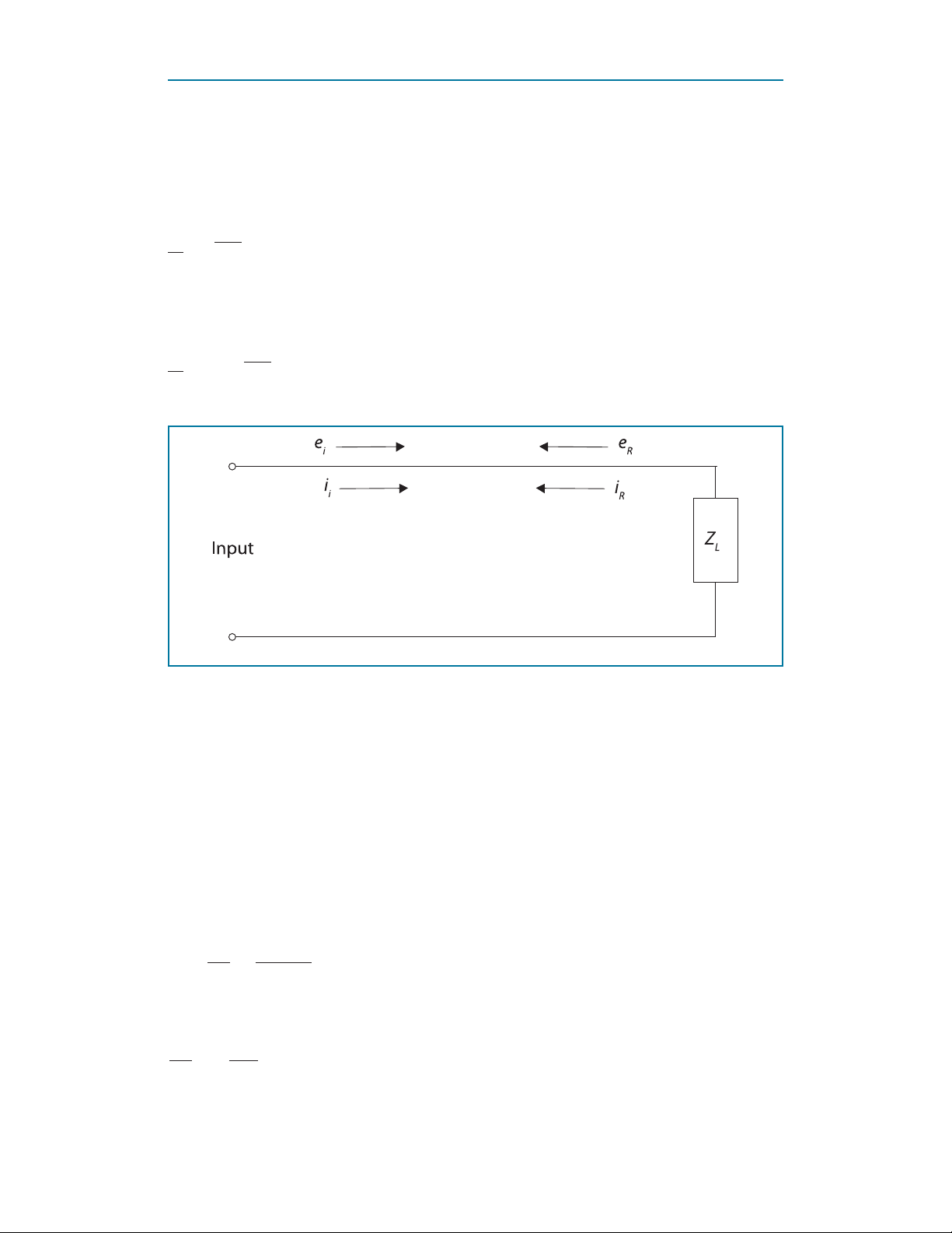
Figure 1.6 Terminated Line
Figure 1.6 shows a line terminated with an impedance load ZL. When a signal is applied
to this line, <100% of the total signal reaches ZL because oa small amount of it is
reected back toward the input. For this reason, the incident current iI ows in the
opposite direction of the reected current iR. So the total current iT felt by the load ZL will
be: iT =iI - iR, but because the direction of the signal does not affect its potential, the total
voltage et felt across load ZL will be: eT = eI +eR. The impedance must equal the total
voltage and the total current. It does not matter if we look at the end load or any other
point along the line.
So:
e
ZL = =
i
We can then restate the equation for ZO as:
e
I
= - = Z
i
I
eI + e
T
T
iI + i
R
R
eR
i
R
0
Microwaves for Everyone | LRL 550B Microwave Training Kit
11
Page 12

introdUCtion – Let’S tALK ABoUt trAnSMiSSion LineS
Now we can see a ratio between incident and reected voltages:
e
e
ZL - Z
R
= = G
I
0
ZL + Z
v
0
This ratio is called the voltage reection coefcient. We can also look at the current
reection coefcient as:
i
Gi = =
i
Z0 - Z
Z0 + Z
L
L
R
I
Let’s look back at the equation: eT = eI + eR. Combining this equation with the
relationships described by the previous equation, we can conclude: eR = GV eI so that
eT = eI + GV eI. When a transmission line experiences a time when the incident and
reected voltages are in phase, this yields a maximum voltage and can be expressed as:
e
= eI (1+ GV ). Equally important is the circumstance when the incident and reected
max
voltages are completely out of phase, which may be expressed as : e
= eI (1- GV ).
min
The relationship that these two points in time share is known as VSWR, or voltage
standing wave ratio, expressed as:
e
VSWR = =
e
max
min
1+ G
1- G
V
V
or simply:
GV =
VSWR - 1
VSWR + 1
VSWR is very useful in determining how well a load is matched to the signal source.
This fact is very important because most signal sources suffer damage when not
properly “loaded”. Since the maximums and minimums take place alternately, every
half wavelength VSWR is helpful in matching loads to frequency. Shown by:
12
u
ƒ =
l
We can also use this ratio to give us the amount of reected power.
GP = = | GV | 2 = | Gt |
rR
2
rI
Consequently, the relationship of the power standing wave ratio and the voltage
standing wave ratio is: PSWR = ( VSWR ) 2. Now we can consider how much power is really
used by the load. More commonly referred to as the loads’ transmission
coefcient voltage, current and power coefcients t are expressed as follows:
tv + Gv = 1
ti + Gi = 1
+ Gp = 1
t
p
tp = | tv | 2 = | ti |
2
Microwaves for Everyone | LRL 550B Microwave Training Kit
Page 13
Up to now, everything we have talked about applies to all types of transmission lines.
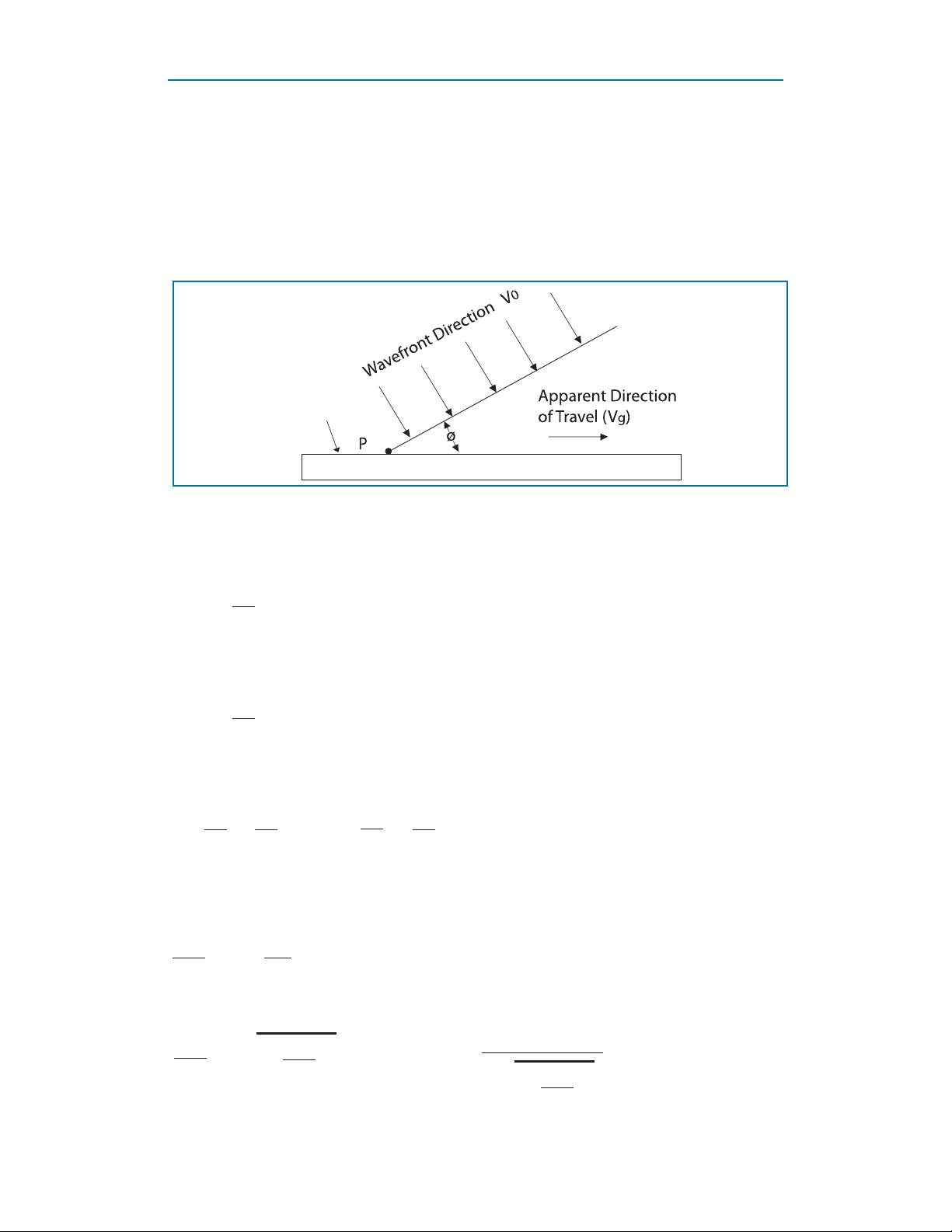
In the experiments that follow, we will be using only waveguide lines. In wave guide
velocity, surfaces and physical dimensions enter the picture; so lets talk about this by
looking at Figure 1.7.
Figure 1.7 Wave Travel along a Surface
Looking only at the RF wave that is traveling near the surface, the velocity Vg is expressed:
V
sin Q =
0
V
g
But when a wave front enters the waveguide at angle Q we see the wavelength of the
RF wave and the physical dimension “a” of the waveguide are expressed:
l
cos Q =
Because the frequency in free air is the same as the frequency inside the waveguide,
frequency can be expressed:
ƒ = =
when V 0 is free air and V g is waveguide velocity. The wavelengths are l
Because: sin
2
l
0
l
g
taking the square root of each side gives:
l
0
l
g
0
2
a
V
l
V
0
0
= 1 -
g
l
g
2
Q = 1 - cos 2 Q
l
0
2
a
l
= 1-
√
( )
2
a
and
2
0
V
V
2
l
0
g
or
0
= = sin Q
l
g
l
g
l
=
0
l
1-
√
( )
2
and l
0
0
2
a
g .
Microwaves for Everyone | LRL 550B Microwave Training Kit
13
Page 14
MeASUreMent oF MiCroWAVe PoWer – eXPeriMent 1
EXPERIMENT 1
Introduction
Microwave power is made up of the same things that make up power at any frequency.
Voltage and current owing through a load E x I =P. The problem in measuring
microwaves results from the fact that most high frequencies cannot be measured with
standard voltmeters or standard current meters. So in the experiment, we will explain the
most popular form of measuring microwaves.
Discussion
When microwaves are absorbed by most materials, they tend to heat up; if they have a
negative or positive temperature coefcient, their base resistance decreases or
increases. This fact becomes very useful because these materials can be utilized to
make a device called a bolometer.
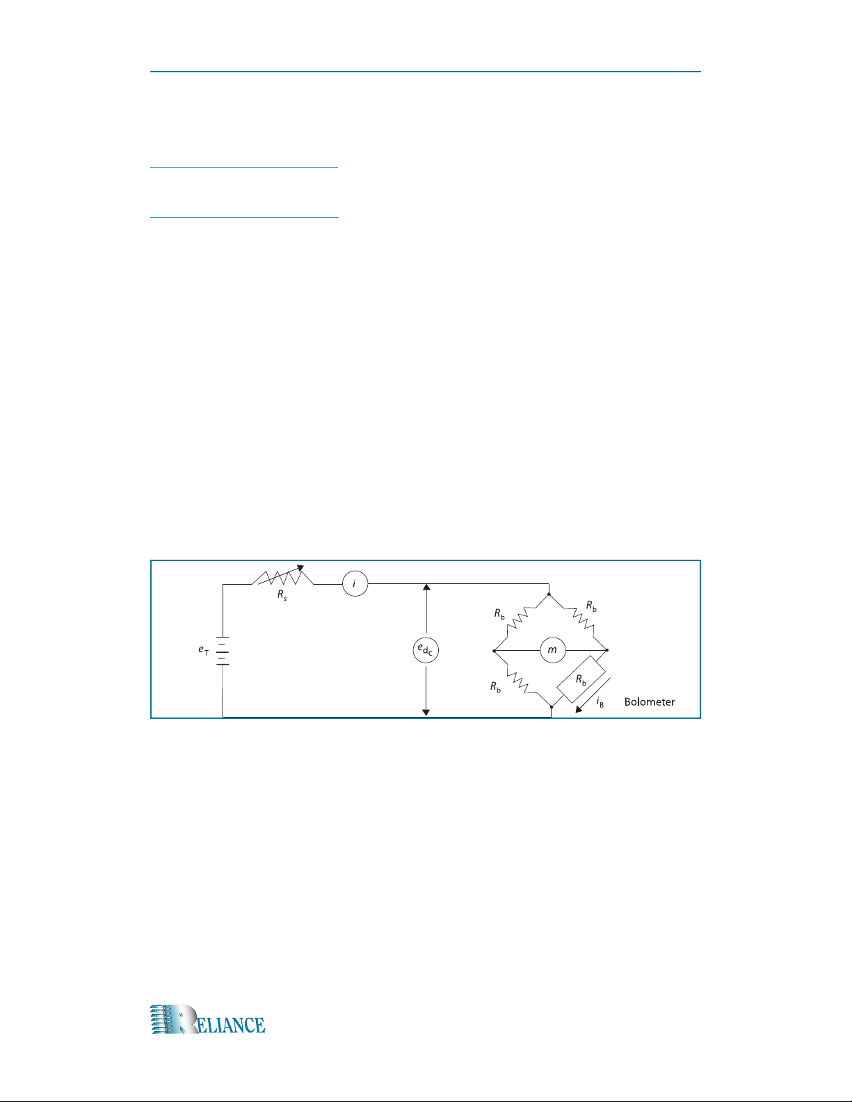
We can use a bolometer as one leg of a bridge network (Figure 1.1) to monitor changes
in resistance.
Bolometer
Figure 1.1 Simple Power Bridge
We see that the total current iT can be adjusted with the potentiometer labeled Rs. When
we use Rs to adjust the current to balance the brige half of the TOTAL current will ow
through Rb, our bolometer.
So we see:
iB = ½ i
T
14
Power will be expressed:
PT = i
2
Rb = ¼ i
B
2
R
T
b
Microwaves for Everyone | LRL 550B Microwave Training Kit
Page 15
Now let’s apply RF power to Rb. It gets hot, and its resistance changes; now the bridge
is no longer balanced. When we adjust Rs to balance the bridge again, the total current
changes. This DC power change is equal to the RF power already applied. DC power is
seen as:
PDC = ½ i
DC
2
R
b
so RF power is the difference between pt and pDC. shown:
PRF = PT – P
DC
This is equal to:
2
PRF = ¼ Rb ( i
T
– i
DC
2
)
Another way of expressing this relationship is:
PRF = ¼ Rb ( iT – i
) ( iT + i
DC
DC
)
Now we want to express:
( iT – i
) by D i
DC
Therefore:
PRF = ¼ Rb ( iT + i
DC
) D i
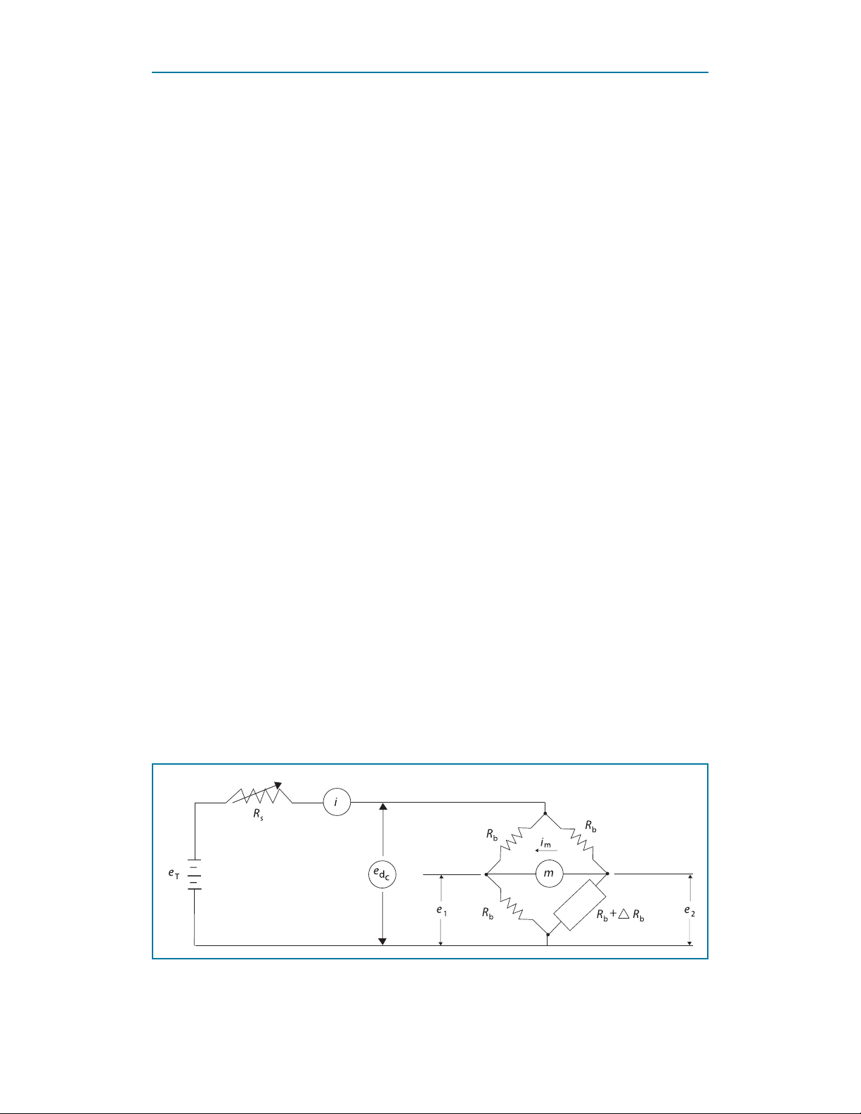
The power bridge in Figure 1.1 is acceptable for measurements when RF power is
1mw or above, but when it goes below 1mw, Di becomes difcult to deal with. A better method of measurement is shown in Figure 1.2 where the voltages e1 & e2 are read
across the meter as:
em = e2 – e
1
Figure 1.2 Directly Calibrated Bridge
Microwaves for Everyone | LRL 550B Microwave Training Kit
15
Page 16

MeASUreMent oF MiCroWAVe PoWer – eXPeriMent 1
Now that current is small enough to ignore, we see:
e1 = e
Or: use the common denominator
and: If is very small
using ohm’s law on the meter:
4 Rb + 2 DR
im = em / R
So:
Rb
DC
2R
em = eDC
em = e
b
m
im ≈ ( DR )
4RbR
and
b
Rb + DR
( )
2Rb + DR
( )
DC
4Rb + 2DR
≈ 4 R
b
e
DC
m
DR
and
b
b
b
e2 = e
–
b
em ≈ e
Rb + DR
( )
DC
2Rb + DR
R
b
2R
b
( )
DC
DR
DR
4R
b
b
b
b
b
16
Now the meter reading is directly proportional to the bolometer resistance.
Equipment and Components
• 1 Microwave RF source (supplied- 510A).
• 1 Thermistor mount (supplied- 508).
• 2 RF attenuators (supplied- 506).
• 3 1000 ohm 1% metal lm; 1/2 watt resistors
• 1 10K ohm potentiometer
• 1 0-30 volt DC power supply
• 2 Volt-ohm meters
Microwaves for Everyone | LRL 550B Microwave Training Kit
Page 17

PLEASE READ CAUTIONS CAREFULLY
BEFORE CONTINUING
CAUTION 1:
Klystrons get extremely hot when in use and must not
be handled while hot! Serious burns can result.
CAUTION 2:
Klystron mount, power supplies, and Klystron tube
plate caps have high voltages present when in use.
Exercise extreme CAUTION!
Shock or death can result.
CAUTION 3:
RF power levels in this kit are not harmful, but a
human eye may be damaged by low levels of
radiation.
Do not look into any waveguide at any time when
units are on.
Microwaves for Everyone | LRL 550B Microwave Training Kit
17
Page 18
MeASUreMent oF MiCroWAVe PoWer – eXPeriMent 1
SEE CAUTION ON PREVIOUS PAGE
Objective
To show the relationship between a thermistor’s resistance cold and when RF power is
applied.
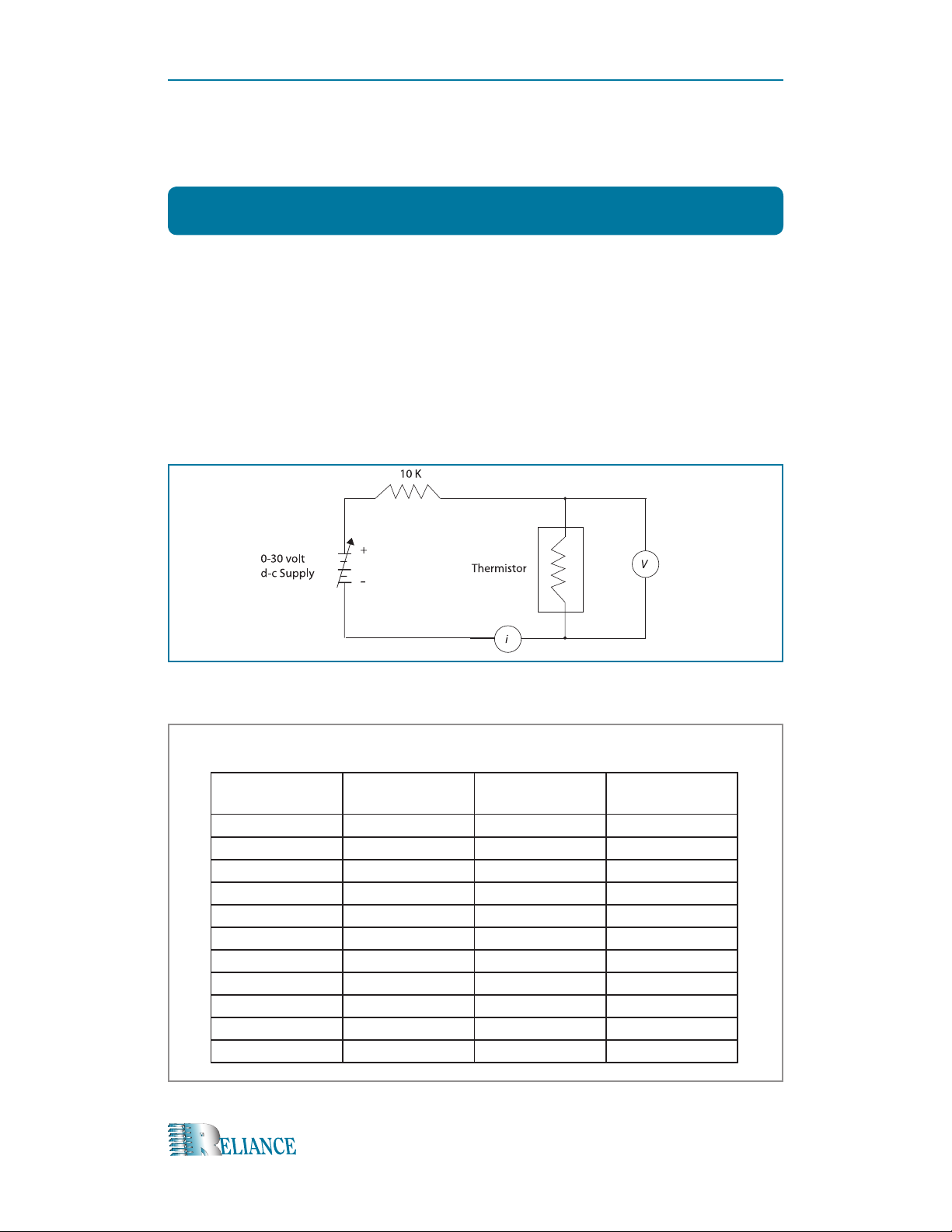
Part 1
1. Hook up circuit in Figure 1.3.
2. Fill in Table 1-1 starting at zero volts and not exceeding 1 volt.
Record the currents rst.
Figure 1.3 Set-up for Determining a Thermistor Volt-Ampere Characteristic
Table 1.1 Data for Procedure, Part 1
Thermistor
Voltage
0.0
0.1
0.2
0.3
0.4
0.5
0.6
0.7
0.8
0.9
1.0
Thermistor
Current
Thermistor
Power
Thermistor
Resistance
18
Microwaves for Everyone | LRL 550B Microwave Training Kit
Page 19
The thermistor element as such cannot be removed from the waveguide mount.
However, its two terminals are readily accessible through the (BNC) connector mounted
on top of the guide.
Under no condition should the student try to remove the thermistor element. Note: Show
Thermistor Voltage from 0.0 up to 1.0 volt. DO NOT GO BEYOND 1.0 VOLT.
3. Then calculate the power readings.
4. Then calculate the resistance readings.
5. Using information from Table 1-1 plot a volt ampere curve.
6. Then plot a power verses resistance curve.
Part 2
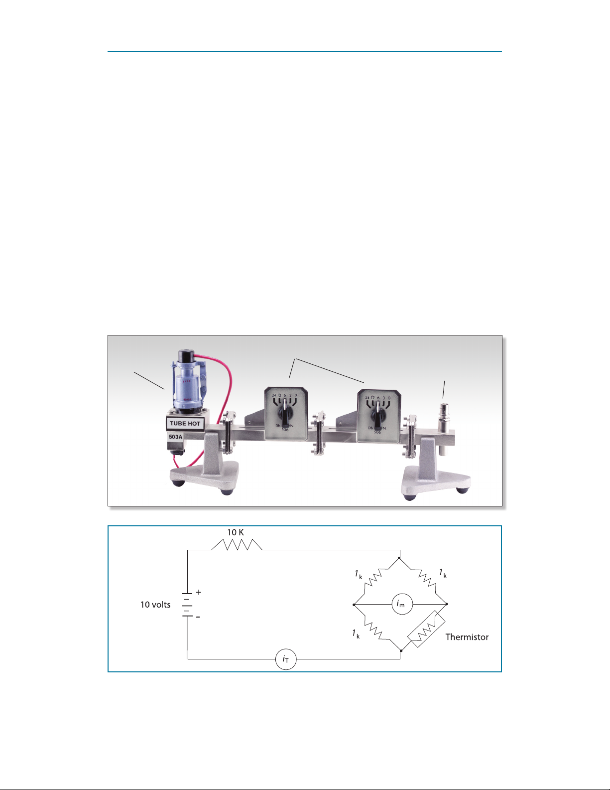
1. Hook up circuit in Fig. 1.4.
506
503A
508
Figure 1.4 Simple RF Power Bridge
Microwaves for Everyone | LRL 550B Microwave Training Kit
19
Page 20
MeASUreMent oF MiCroWAVe PoWer – eXPeriMent 1
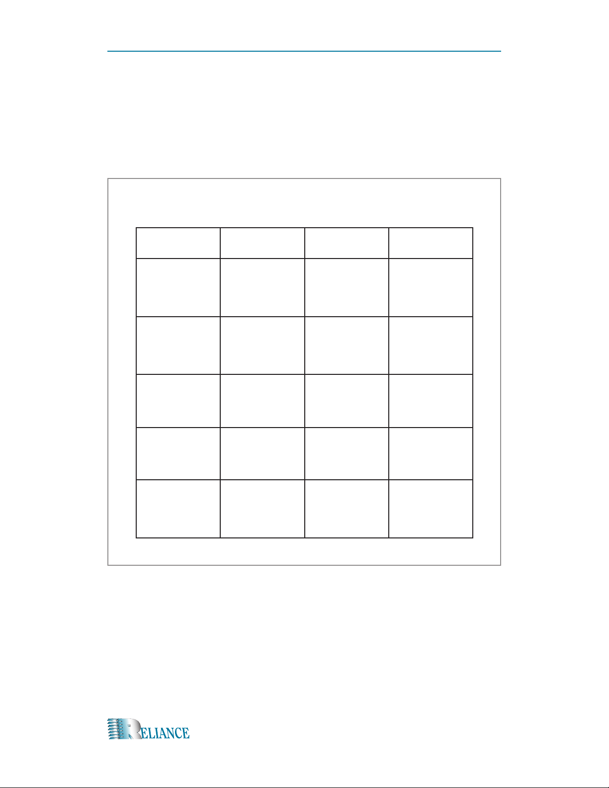
2. Balance the bridge with 10 K ohm potentiometer (This is zero current through
meter im).
3. Enter reading from meter iT as total current iT on Table 1.2.
Table 1.2 Data for Procedure, Part 2
i
T
i
m
i
DC
RF
Power
20
The thermistor element as such cannot be removed from the waveguide mount.
However, its two terminals are really accessible through the (BNC) connector mounted
on top of the guide.
Under no condition should the student try to remove the thermistor element.
4. Apply RF power to bridge as in Figure 1.5 keeping attenuators with full ap
insertion (maximum attenuation). Enter reading from im in Table 1.2.
Microwaves for Everyone | LRL 550B Microwave Training Kit
Page 21
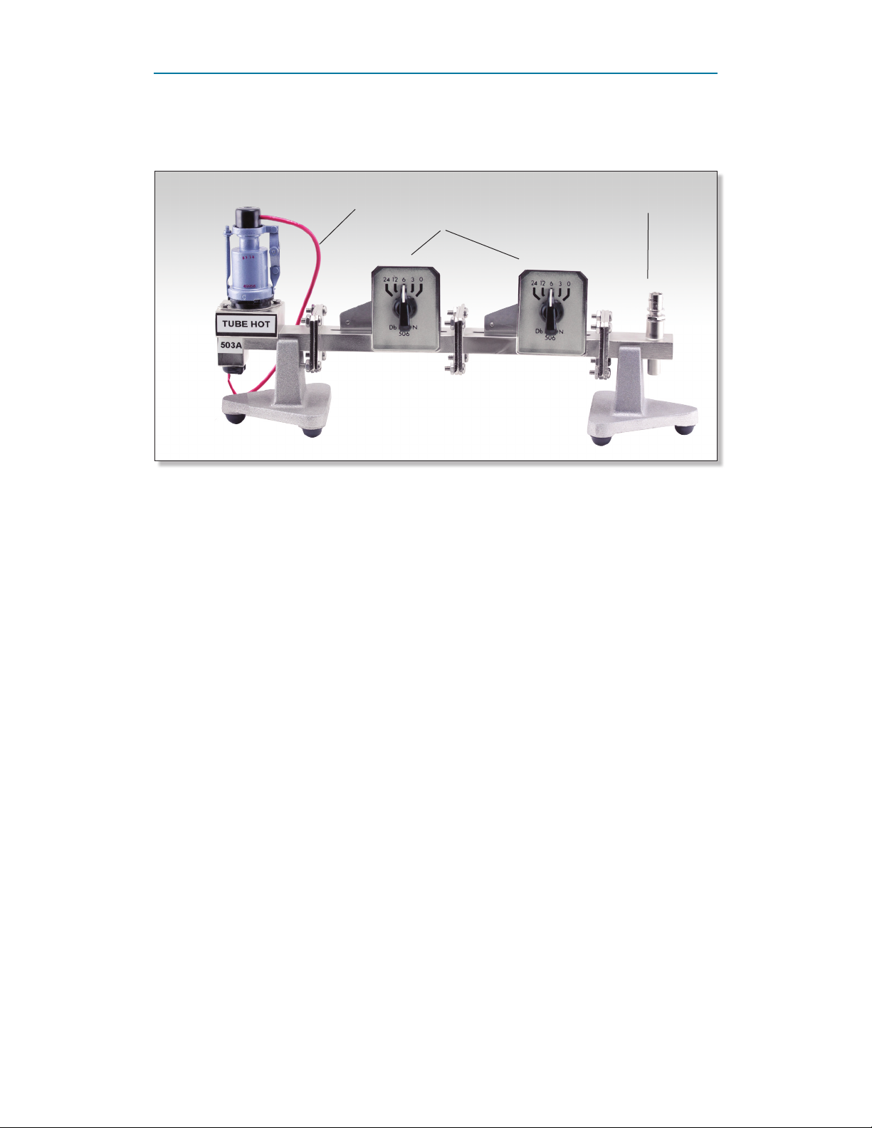
503A
506
508
5. Enter reading of new total current iDC in Table 1.2.
6. Calculate and enter reading of RF power in Table 1.2.
7. Adjust RF attenuators for less attenuation; then repeat steps 2-6.
8. Take three more readings at new RF inputs (adjusting the attenuators) repeating
steps 2 - 6 each time.
9. Now you can plot a curve showing RF power and bridge current im.
Microwaves for Everyone | LRL 550B Microwave Training Kit
21
Page 22
MeASUreMent oF VoLtAGe StAndinG WAVe rAtio – eXPeriMent 2
EXPERIMENT 2
Introduction
When RF is transmitted down a line into a load, even one with a good match, some of
the signal reects back toward the source. The amount of signal sent vs. the amount
reected back is compared and referred to as the standing wave ratio. When this pattern
deals with measurements of voltage, it is called the voltage standing wave ratio (VSWR),
it is simply expressed as:
e
VSWR =
e
max
min
Discussion
e
The equation of VSWR =
would be very easy to use to calculate VSWR if the voltage measurements were as easy
to take, but they are not.
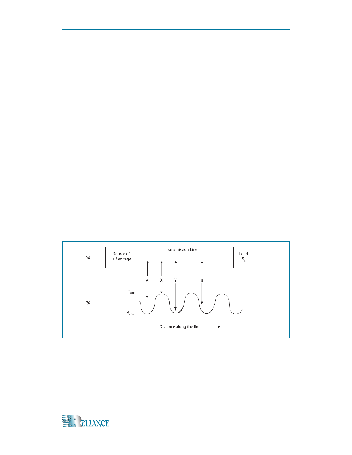
The most popular method of measuring VSWR employs the use of a slotted line. To help
us understand this device, let us look at Figure 2.1a.
VSWR =
max
e
min
22
Figure 2.1 Voltage Distribution along a Transmission Line
This diagram shows us a sample length of transmission line, in our case X-band waveguide. In Figure 2.1b, we see an expanded view of the RF sine wave rising and falling
along the length of the line. Placing a slotted line into the transmission line from point
A to point B allows us to inspect a probe into the slot in the line. We can then move the
probe along the line reading peaks and dips, e
Because RF voltages are so difcult to measure, we will make the probe like the one in
Figure 2.2a.
Microwaves for Everyone | LRL 550B Microwave Training Kit
max
and e
which are shown as X and Y.
min
Page 23
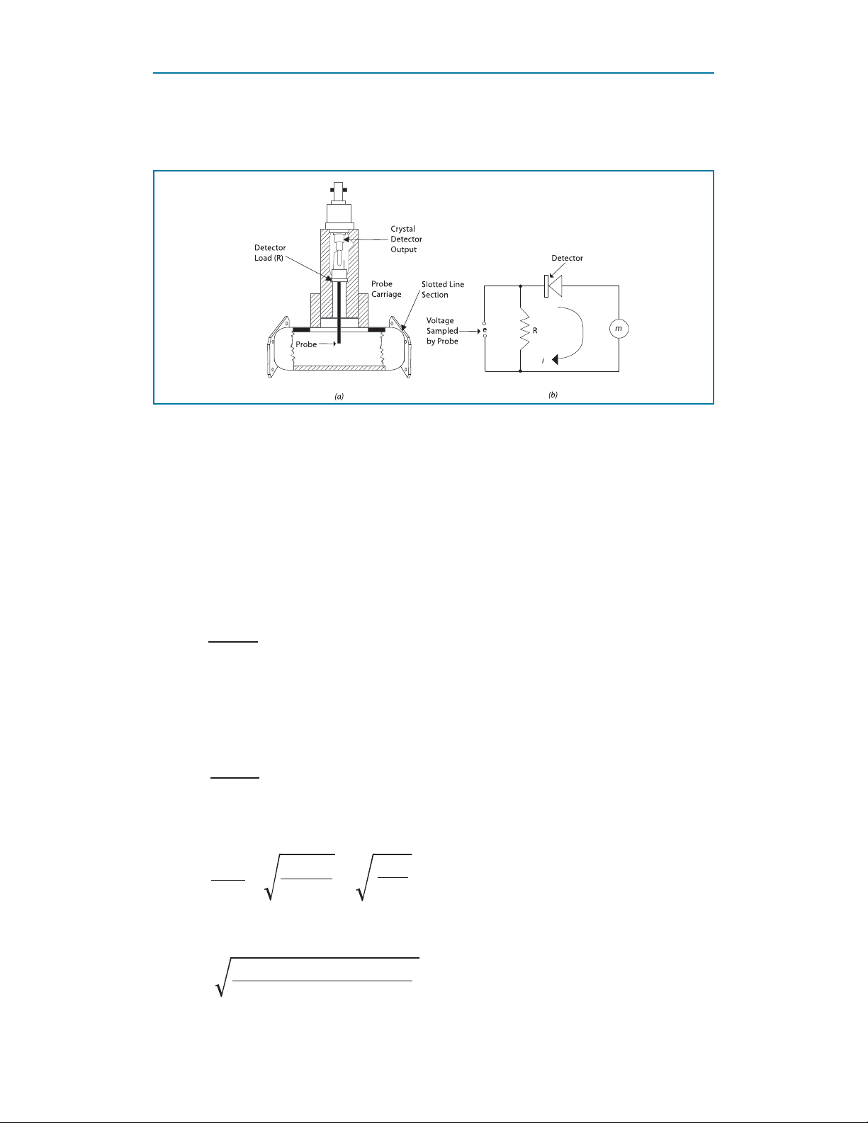
Figure 2.2 Slotted Transmission Line and Probe (a) Cutaway Sketch of a Slotted Section
with Probe, Carriage, and Detector (b) Equivalent Detector Circuit
The key addition here is the crystal detector which will change the RF voltage into a DC
current and will be read by the meter in Figure 2.2b. Because some detectors act differently from others, we will use a “square law” detector. These detectors have an output
proportional to the square of the input. So if we place the probe at Y on the slotted line,
we will get:
i
min
= ke
min
2
Or:
e
min
= √ i
min
/ k
Then if we move the probe to point X, we get:
i
max
= ke
max
2
Or:
e
max
= √ i
max
/ k
Together we get:
i
e
VSWR = = =
e
max
min
max
i
max
/ k
/ k
i
max
i
min
Now we can measure the X and the Y on the meter in Figure 2-2b and we see:
VSWR =
maximum meter reading
minimum meter reading
Microwaves for Everyone | LRL 550B Microwave Training Kit
23
Page 24
MeASUreMent oF VoLtAGe StAndinG WAVe rAtio – eXPeriMent 2
This way of measuring VSWR is by far the easiest, but if the minimum meter reading
cannot be measured with a reliable degree of accuracy, the inherent aws in the detector
may create distortion increasing the chance of error.
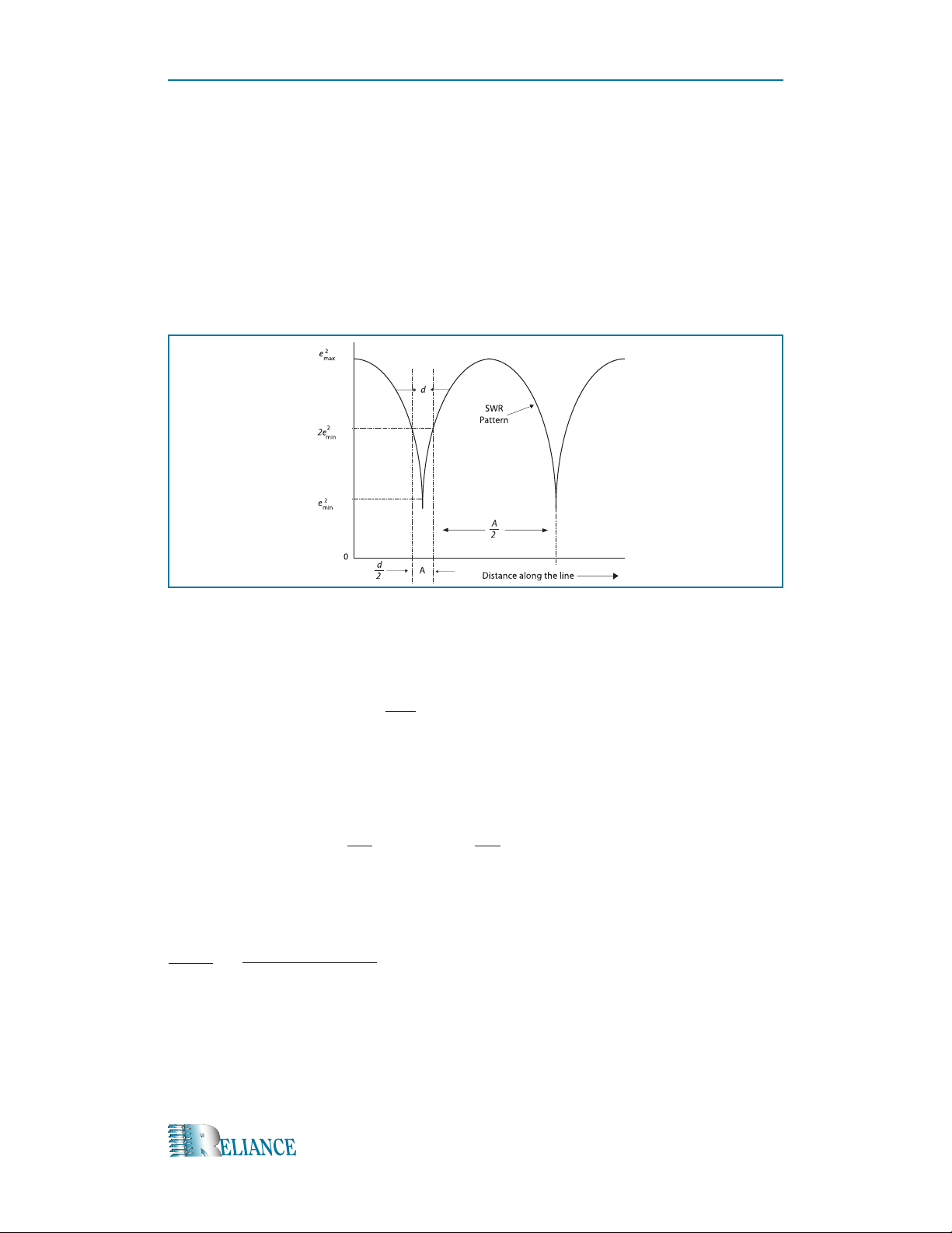
When standing wave ratios are larger than ten to one, the “double minimum” measurement system can be used to in crease the accuracy and reduce the percentage of error.
Let us examine this method in Figure 2.3.
Figure 2.3 Double Minimum Method
The mathematical expression of this curve is:
pd
l
2pl
( )
l
min
2
sin
pd
2
( )
l
e = e
starting at point “A”, we move to the right until the reading is twice what it was at point
“A”. This gives us:
2e
This relationship can also be expressed as:
Because in mathematics:
2
+ (e
min
2
= e
min
2
e
max
=
2
e
min
min
max
2
+ e
2
2
– e
) sin2
min
2
sin – e
max
1 + sin2 ( p d / l )
2
( d / l )
sin
( )
sin 2 Q = 1-cos 2 Q
24
Microwaves for Everyone | LRL 550B Microwave Training Kit
Page 25

we can restate the formula as:
2
e
max
e
min
and also as:
2 – cos 2 ( p d / l )
=
2
sin
2
( p d / l )
e
VSWR = =
The actual measurement of VSWR, however, is done by measuring the distance between
two “double minimum” measurements. Then we use this information and a trigonometric
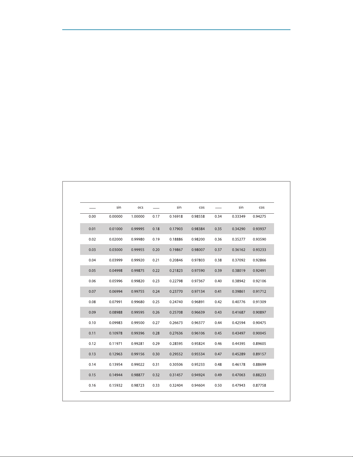
table like the one in Table 2.2.
VSWR’s with ten or greater angle pd/l will be small and so will sin (p d/ l) because of
this:
e
max
min
√ 2 – cos 2 ( p d l )
sin ( p d / l )
1 + sin2 ( p d / l ) ≈ 1
So then:
1
VSWR ≈
because of the small angle:
sin ≈
( )
Now we can reduce this equation to:
sin ( p d / l )
p d
l
p d
l
l
VSWR ≈
p d
This is only required when VSWR is greater than ten. In some cases, the measurements
of e
max
and e
can be amplied to provide better accuracy.
min
Equipment and Materials
• 1 Microwave source (supplied- 510A).
• 2 Waveguide attenuators (supplied- 506).
• 1 Slotted line with probe and detector (supplied- 505).
• 1 DC microammeter (supplied).
• 1 Short circuit terminator (supplied- 503A).
• 2 Waveguide stands (supplied- 523).
Microwaves for Everyone | LRL 550B Microwave Training Kit
25
Page 26
MeASUreMent oF VoLtAGe StAndinG WAVe rAtio – eXPeriMent 2
PLEASE READ CAUTIONS CAREFULLY
BEFORE CONTINUING
CAUTION 1:
Klystrons get extremely hot when in use and must not
be handled while hot! Serious burns can result.
CAUTION 2:
Klystron mount, power supplies, and Klystron tube
plate caps have high voltages present when in use.
Exercise extreme CAUTION!
Shock or death can result.
CAUTION 3:
RF power levels in this kit are not harmful, but a
human eye may be damaged by low levels of
radiation.
Do not look into any waveguide at any time when
units are on.
26
Microwaves for Everyone | LRL 550B Microwave Training Kit
Page 27
SEE CAUTION ON PREVIOUS PAGE
Objective
In this experiment, we will look at some common ways to measure VSWR.
Part 1 • Medium VSWR
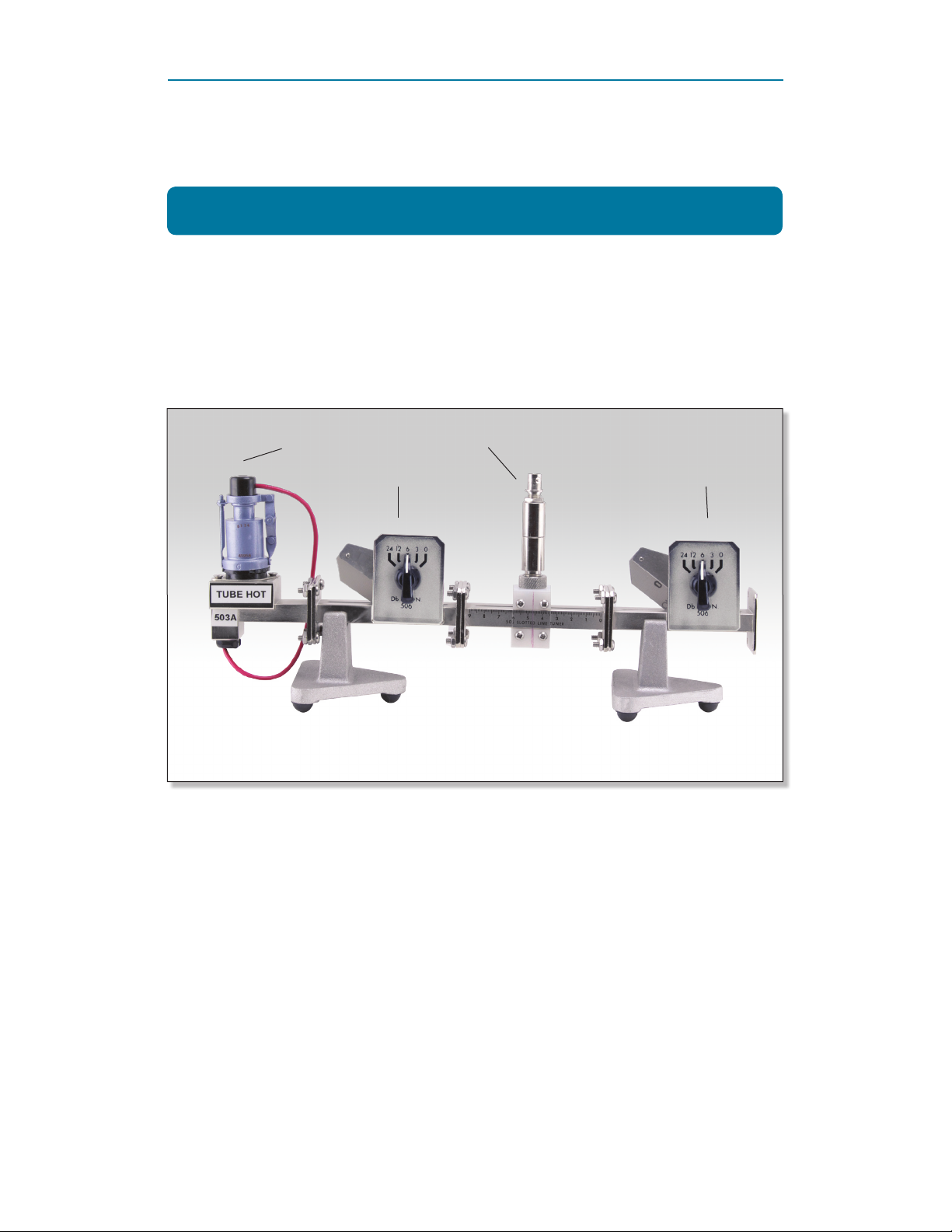
1. Set up test xture in Figure 2.4.
503A
506
2. Connect one of the video cables from the detector on the slotted line to the input
marked VSWR on the power supply.
3. Turn on power supply and apply RF power.
505
506
4. Move probe on slotted line and adjust for maximum deection (try to keep this at
the center of the slotted line if possible).
5. With the shorted attenuator set at maximum, adjust the RF feed attenuator for a
close to full scale reading.
6. Move the probe for a minimum reading.
7. Adjust the short feed attenuator for a reading of about 1/4 scale.
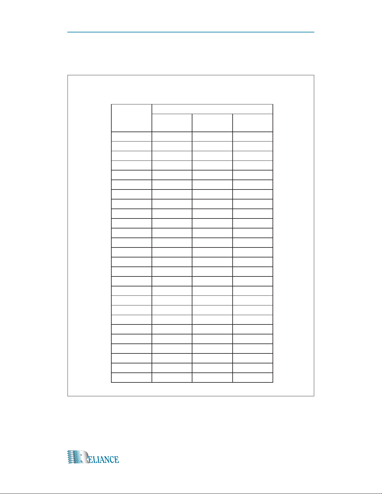
8. Measure and record the readings at the points indicated on Table 2.1.
Microwaves for Everyone | LRL 550B Microwave Training Kit
27
Page 28
MeASUreMent oF VoLtAGe StAndinG WAVe rAtio – eXPeriMent 2
Table 2.1 Data
Distance
along the
Line (in cm)
0.0
0.2
0.4
0.6
0.8
1.0
1.2
1.4
1.6
1.8
2.0
2.2
2.4
2.6
2.8
3.0
3.2
3.4
3.6
3.8
4.0
4.2
4.4
4.6
4.8
5.0
Meter Readings in u amp
Part 1 Part 2 Part 3
28
9. Plot a curve of distance and readings.
10. Using Table 2.2 and equations from the discussion section, ll in the VSWR
calculations on Table 2.1.
Microwaves for Everyone | LRL 550B Microwave Training Kit
Page 29
Part 2 • High VSWR
1. Use the same test xture and adjust the RF feed attenuator to minimum
attenuation.
2. Move the probe to minimum reading and then adjust the short attenuator for a
reading of 1 /10 full scale.
3. Repeat steps 8, 9, and 10 of part 1 (record any off scale readings as off scale).
Part 3 • Low VSWR
1. Adjust short attenuator to maximum attenuation.
2. Adjust RF feed attenuator for a 50% of full scale with probe at a peak point.
3. Repeat steps 8, 9, and 10 of part 1.
Table 2.2
πd
λ
0.00 0.00000 1.00000 0.17 0.16918 0.98558 0.34 0.33349 0.94275
0.01 0.01000 0.99995 0.18 0.17903 0.98384 0.35 0.34290 0.93937
0.02 0.02000 0.99980 0.19 0.18886 0.98200 0.36 0.35277 0.93590
0.03 0.03000 0.99955 0.20 0.19867 0.98007 0.37 0.36162 0.93233
0.04 0.03999 0.99920 0.21 0.20846 0.97803 0.38 0.37092 0.92866
0.05 0.04998 0.99875 0.22 0.21823 0.97590 0.39 0.38019 0.92491
0.06 0.05996 0.99820 0.23 0.22798 0.97367 0.40 0.38942 0.92106
0.07 0.06994 0.99755 0.24 0.23770 0.97134 0.41 0.39861 0.91712
0.08 0.07991 0.99680 0.25 0.24740 0.96891 0.42 0.40776 0.91309
0.09 0.08988 0.99595 0.26 0.25708 0.96639 0.43 0.41687 0.90897
0.10 0.09983 0.99500 0.27 0.26673 0.96377 0.44 0.42594 0.90475
0.11 0.10978 0.99396 0.28 0.27636 0.96106 0.45 0.43497 0.90045
0.12 0.11971 0.99281 0.29 0.28595 0.95824 0.46 0.44395 0.89605
0.13 0.12963 0.99156 0.30 0.29552 0.95534 0.47 0.45289 0.89157
0.14 0.13954 0.99022 0.31 0.30506 0.95233 0.48 0.46178 0.88699
sin ocs sin cos sin cos
πd
λ
πd
λ
0.15 0.14944 0.98877 0.32 0.31457 0.94924 0.49 0.47063 0.88233
0.16 0.15932 0.98723 0.33 0.32404 0.94604 0.50 0.47943 0.87758
Microwaves for Everyone | LRL 550B Microwave Training Kit
29
Page 30

MeASUreMent oF FreQUenCY And WAVeLenGtH – eXPeriMent 3
EXPERIMENT 3
Introduction
Microwaves differ from standard RF because they consist of extremely high frequency
waves. Consequently, in order to understand microwaves, we must understand
microwave frequency measurements. In this experiment, we will look at some
common ways to measure microwave frequency.
Discussion
The relationship of a RF wave could be seen as an equation between frequency,
wavelength, and velocity:
ƒ l = V
Frequency remains xed in our equation so that wavelength is directly affected by the
velocity. The velocity of our wave is determined by its physical path of travel if the wave
is traveling through air, velocity is equal to: V
When it travels along paths other than air, the velocity is affected by other factors, as
expressed:
V
0
√et m
t
Here, etequals the permitivity of the path, and mt equals the permeability of the path e
and mt are different for different materials, and these factors can be found in microwave
engineering guides or handbooks. Since we are considering velocity to be a constant
through a given path, frequency and wavelength can be measured.
We will look at two methods of measuring frequency and wavelength; any one of the two
can be used to calculate the other.
First, let us look at the slotted line to measure wavelength. Look at the wave in Figure 3.1.
= 3 x 10
0
10
cm per sec
t
30
Microwaves for Everyone | LRL 550B Microwave Training Kit
Page 31
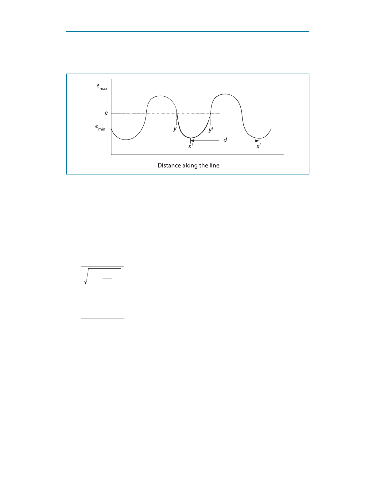
Figure 3.1 Distance along the Line
The distance “d” between c1 and c2 is represented by the equation l
= 2 d, lL is equal
L
to the wavelength as measured along the slotted line. When using a coaxial line, velocity
V
will be about equal to air velocity V0. so we see that l
L
= lO.
L
When using waveguide, velocity is determined by the larger dimension “a” (Table 3-3 in
this chapter will assist you with the values for “a”). We can compare the wavelength in
waveguide to the wavelength of “air” by:
l0
lL =
l
0
1 –
2
2a
Then we calculate:
2
L
2a l
2
+ 4a
L
min
.
V0 √ l
ƒ =
These equations work well in calculating frequency and wavelengths as long as “d” can
be measured with little problem.
So when we have a high VSWR on the line (ve or more), there is no problem, but a low
VSWR makes c1 and c2 difcult to locate (refer to Figure 3.1). We can select a value for
e any value larger than e
X1 will be at the center of measurements of e shown as y and y1.
This is shown:
y' + y
c1 =
Microwaves for Everyone | LRL 550B Microwave Training Kit
2
31
Page 32

MeASUreMent oF FreQUenCY And WAVeLenGtH – eXPeriMent 3
PLEASE READ CAUTIONS CAREFULLY
BEFORE CONTINUING
CAUTION 1:
Klystrons get extremely hot when in use and must not
be handled while hot! Serious burns can result.
CAUTION 2:
Klystron mount, power supplies, and Klystron tube
plate caps have high voltages present when in use.
Exercise extreme CAUTION!
Shock or death can result.
CAUTION 3:
RF power levels in this kit are not harmful, but a
human eye may be damaged by low levels of
radiation.
Do not look into any waveguide at any time when
units are on.
32
Microwaves for Everyone | LRL 550B Microwave Training Kit
Page 33

We see a much improved accuracy if we take several readings on the slotted line for “d”,
and then take the average of “d” and use it in place of “d” when using the equation to
calculate wavelength.
The next method of measuring frequency and wavelength is a resonant cavity. In this
type of measurement, we monitor the power owing through the cavity and adjust the
internal plunger until a “dip” is seen on the power meter. The point of lowest power is
the point of resonance. Some cavities come with calibration charts so the frequency
can be read right off the chart. Others are marked in frequency and can be read direct.
Another way to use this approach is to know the frequency fo and set the plunger to the
setting R0. When the cycles per dial division are known, we can use the different plunger
settings shown Df to calculate the new frequency:
ƒ = ƒ0 + D ƒ ( R0 – R)
As an example, we might establish that a setting of “550” is equal to 9.0 kmc and that
every dial division equals a difference of 5.0 mc. if the plunger setting changes to “345”.
What is the new frequency?
Let’s see:
ƒ = 9 x 10
9
+ 5 x 10
6
( 550–345 ) cps
ƒ = 9 x 10 9 + 1.025 x 10 9 cps
ƒ = 10.025 x 10 9 cps = 10.025 kmc
Our new frequency is now 10.025 kmc.
Equipment and Components
• 1 Microwave RF source (supplied- 510A).
• 2 Adjustable waveguide attenuators (supplied- 506).
• 1 Cavity wave meter (supplied- 504).
• 1 Termination (supplied- 507).
• 1 RF power bridge (supplied).
• 1 Short circuit termination (supplied- 503A).
• 2 Waveguide stands (supplied- 523).
• 1 Detector mount (supplied- 518).
SEE CAUTION ON PREVIOUS PAGE
Microwaves for Everyone | LRL 550B Microwave Training Kit
33
Page 34
MeASUreMent oF FreQUenCY And WAVeLenGtH – eXPeriMent 3
Objective
To demonstrate both cavity tuned and slotted line frequency and wavelength
measurements.
Part 1. The Cavity Wave Meter.
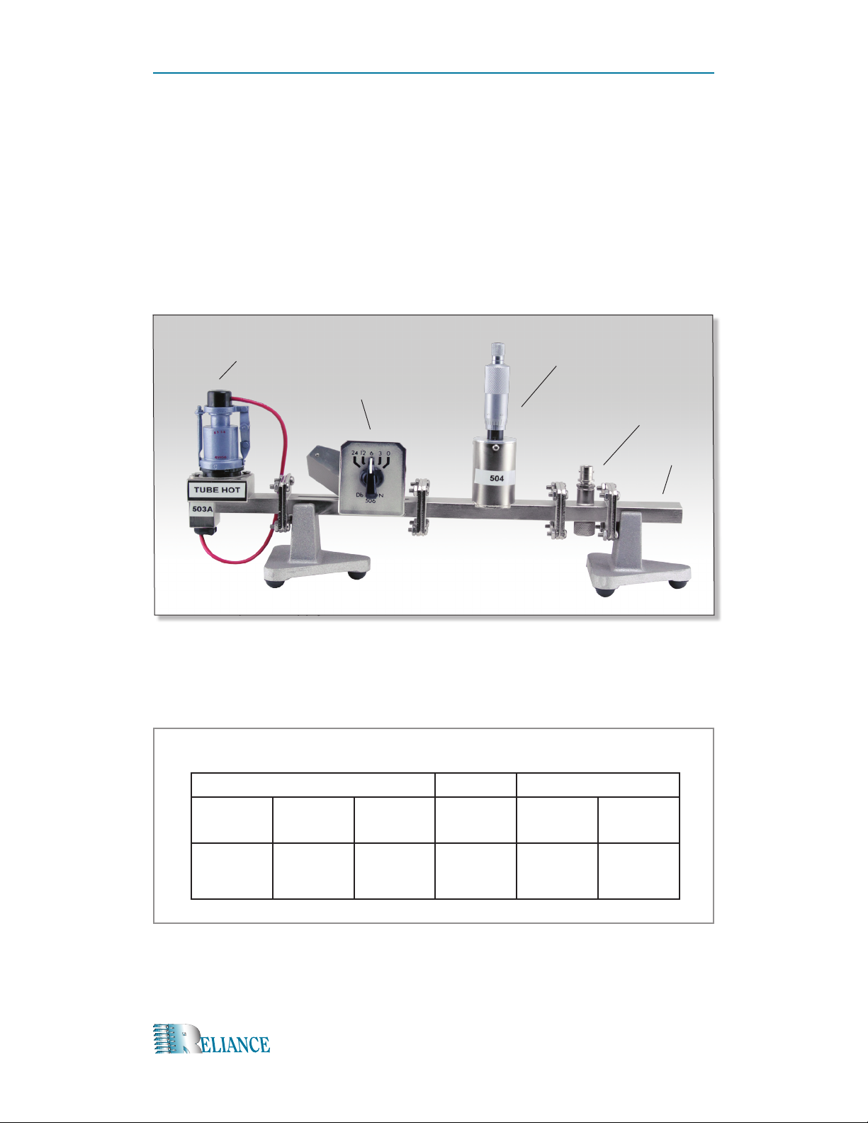
1. Set up Figure 3.2.
503A
506
2. Turn on power supply.
3, Adjust the attenuator for a power reading of at least 50 percent.
4. Starting at a cavity reading of 0.000, slowly tune the plunger until a “dip” is
obtained (this will be the lowest power reading on the meter).
5. Record the reading on Table 3.1.
Table 3.1 Data
504
518
507
34
From Wavemeter At Dip Computed
R
o
6. Record the cavity calibrated point.
7. Record the rate of change per dial increment.
f
o
Microwaves for Everyone | LRL 550B Microwave Training Kit
Δf R f λ
L
Page 35
8. Calculate the frequency of the source.
9. Calculate the wavelength.
Part 2.
1. Replace the cavity with the slotted line.
2. Replace the termination & detector mount with another attenuator (terminated with
a short).
3. Adjust the VSWR for about 1.2.
4. Using the slotted line, complete readings for X1 and X2 and record them in Table 3.2.
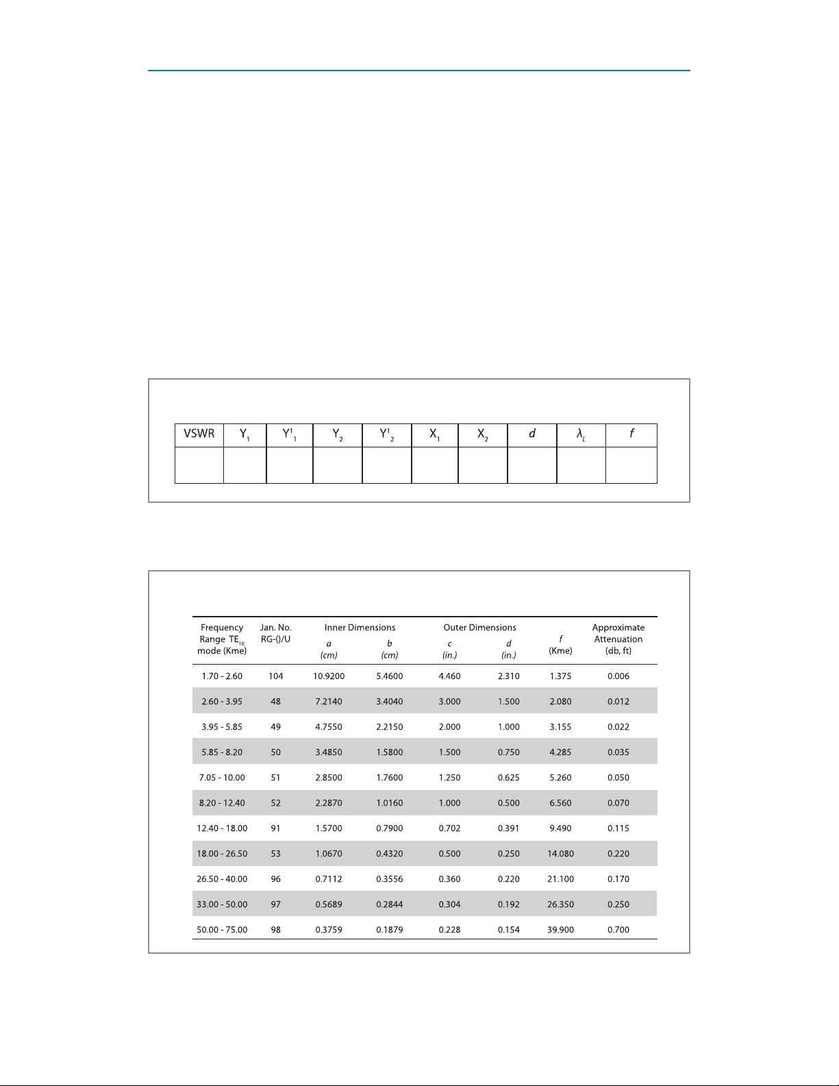
Table 3.2 Data
VSWR Y
1
Y
1
Y
1
2
1
Y
X
2
1
X
2
5. Using Measurements for “low” VSWR, nd Y and Y1.
6. Now calculate for frequency and wavelength.
Table 3.3 Data
Frequency
Range TE
mode (Kme)
1.70 - 2.60 104 10.9200 5.4600 4.460 2.310 1.375 0.006
2.60 - 3.95 48 7.2140 3.4040 3.000 1.500 2.080 0.012
3.95 - 5.85 49 4.7550 2.2150 2.000 1.000 3.155 0.022
5.85 - 8.20 50 3.4850 1.5800 1.500 0.750 4.285 0.035
7.05 - 10.00 51 2.8500 1.7600 1.250 0.625 5.260 0.050
8.20 - 12.40 52 2.2870 1.0160 1.000 0.500 6.560 0.070
10
Jan. No.
RG-()/U
Inner Dimensions Outer Dimensions
a
(cm)
b
(cm)
c
(in.)
d
(in.)
d λ
f
(Kme)
L
Approximate
Attenuation
(db, ft)
f
12.40 - 18.00 91 1.5700 0.7900 0.702 0.391 9.490 0.115
18.00 - 26.50 53 1.0670 0.4320 0.500 0.250 14.080 0.220
26.50 - 40.00 96 0.7112 0.3556 0.360 0.220 21.100 0.170
33.00 - 50.00 97 0.5689 0.2844 0.304 0.192 26.350 0.250
50.00 - 75.00 98 0.3759 0.1879 0.228 0.154 39.900 0.700
Microwaves for Everyone | LRL 550B Microwave Training Kit
35
Page 36
ProPoGAtion oF MiCroWAVeS – eXPeriMent 4
EXPERIMENT 4
Introduction
Microwaves travelling in free space (that is out of the connes of a transmission line) can
be altered and affected by many things. In this experiment, we will try to examine some
of the factors affecting microwaves traveling in free space.
Discussion
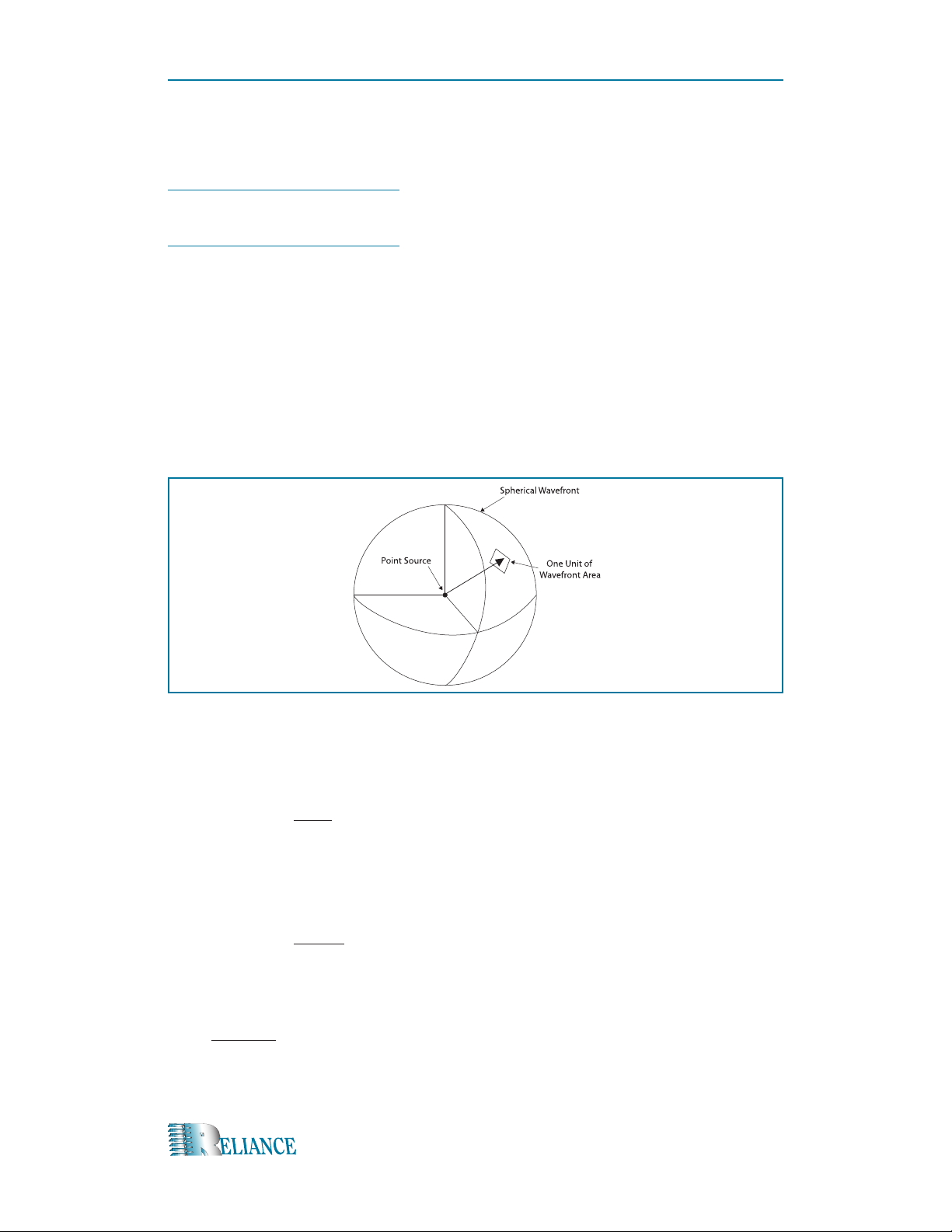
If an RF source is radiating power equally in all directions, then the wavefront moving
away from the starting point will be a sphere. This starting point is known as an “isotropic
point source”, or “point source” to be short. Figure 4.1 shows such a wavefront.
36
Figure 4.1 Spherical Wavefront
Because the total power radiated at the “point source” is spread over the entire sphere,
the power density per unit of the wavefront is the transmitted power Ptr divided by the
area of the sphere:
r
power density =
4p
tr
2
r
where r is not the radius, but the range of the measured area from the point source.
If we concentrate the radiation at the point source by a factor GT (the ratio of the area of
the sphere to the actual area covered), we now get:
r
power density =
4p
tr GT
r
2
If we pick up a portion of the transmission with an antenna, which has an area Ar the
received power is:
r
=
tr GT Ar
2
4p
r
r
rec
This formula describes one of the basic properties of radiated power. When the
transmitted power and the antenna are constant, the received power is proportional to
Microwaves for Everyone | LRL 550B Microwave Training Kit
Page 37
the inverse of the range squared. This relationship is referred to as the “inverse square
law”. A problem appears when we try to make the source appear to be a point source.
To do this, we must use a range that is very large in relationship to the source antenna’s
area. The minimum range to take this measurement is:
2
min
≥
2d
l
0
l
“ is the free-space
o
r
where “d” is the largest dimension of the source antenna, and “
wavelength of the transmitted signal.
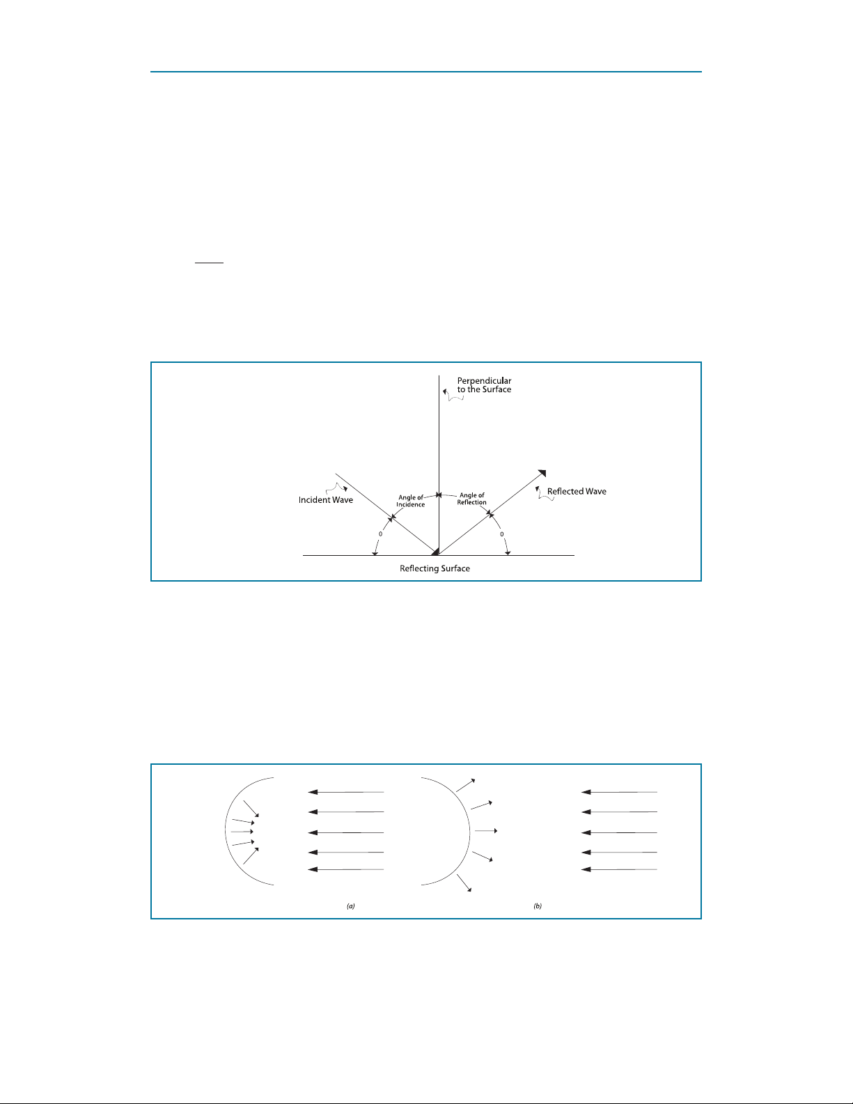
Let us consider the reection of a wave bouncing off a at surface as shown in Figure 4.2.
Figure 4.2 Reection from a Flat Surface
The reected wave has the same angle as the incidence wave with a perpendicular to
the surface. The angle between the incidence wave and the perpendicular is called the
“angle of incidence”. Likewise, the angle between the perpendicular and the reected
wave is called the “angle of reection”. The fact that these two angles are the same
always holds true for a at surface.
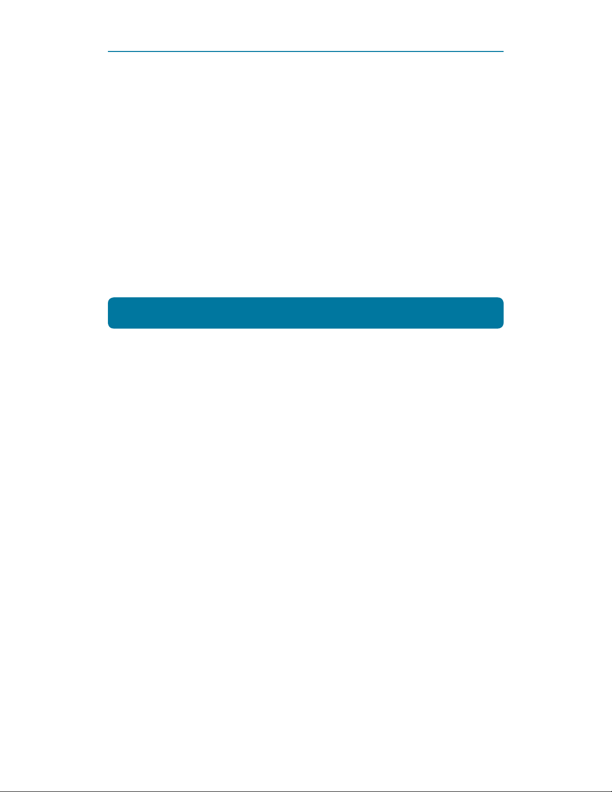
If the surface is not at, but is concave or convex, this rule changes. Figure 4.3 shows
us these two surfaces.
Figure 4.3 Reection from a Curved Surface (a) Concave (b) Convex
Figure 4a shows how a concave surface focuses the reected waves to a xed point,
while Figure 4.3b shows how a convex surface sends them off in many directions.
Microwaves for Everyone | LRL 550B Microwave Training Kit
37
Page 38

ProPoGAtion oF MiCroWAVeS – eXPeriMent 4
PLEASE READ CAUTIONS CAREFULLY
BEFORE CONTINUING
CAUTION 1:
Klystrons get extremely hot when in use and must not
be handled while hot! Serious burns can result.
CAUTION 2:
Klystron mount, power supplies, and Klystron tube
plate caps have high voltages present when in use.
Exercise extreme CAUTION!
Shock or death can result.
CAUTION 3:
RF power levels in this kit are not harmful, but a
human eye may be damaged by low levels of
radiation.
Do not look into any waveguide at any time when
units are on.
38
Microwaves for Everyone | LRL 550B Microwave Training Kit
Page 39
Equipment and Components
• 1 RF microwave source (supplied- 510A).
• 1 Crystal detector (supplied- 518).
• 1 Waveguide termination (supplied- 507).
• 1 Variable attenuator (supplied- 506).
• 2 Waveguide horns (supplied- 531).
• 1 Flat metal surface (not supplied).
• 1 Oscilloscope (optional).
• 4 Waveguide stands (supplied- 523).
SEE CAUTION ON PREVIOUS PAGE
Microwaves for Everyone | LRL 550B Microwave Training Kit
39
Page 40
ProPoGAtion oF MiCroWAVeS – eXPeriMent 4
Objective
To reect and receive a microwave signal.
1. Look at the two waveguide horns. If they are not identical in size, use the smaller
one as the source antenna.
2. Calculate the minimum range to be used. Use the dimensions of the source
antenna and 3 cm as the approximate free-space wavelength.
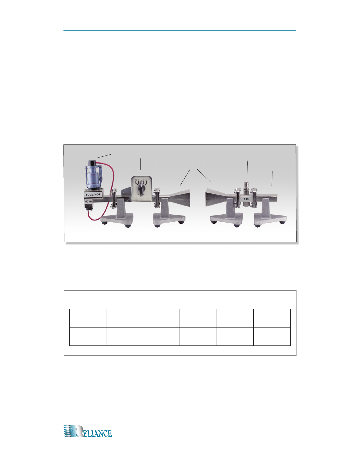
3. Set up the source side of Figure 4.4.
503A
506 518
531
507
4. Set up the receive side of Figure 4.4. Turn on power and allow a warm-up period.
5. Set up receiver directly in line with the source at about 10 times the r minimum.
Record this value in Table 4.1.
Table 4.1 Data
r
min
Initial
Range
Pulse
Height
Range
with 3 dB
Range
with 6 dB
Range
with 9 dB
40
6. Set the attenuator to minimum and record pulse height at the oscilloscope. Record
this in Table 4.1. (if no oscilloscope is available, you can take measurements with
the VSWR portion of your trainer.)
7. Set attenuator for 1/2 pulse height. Then move the receiver closer to the source
until the pulse height is the same as in step 6. Measure and record the new range
in Table 4.1.
Microwaves for Everyone | LRL 550B Microwave Training Kit
Page 41
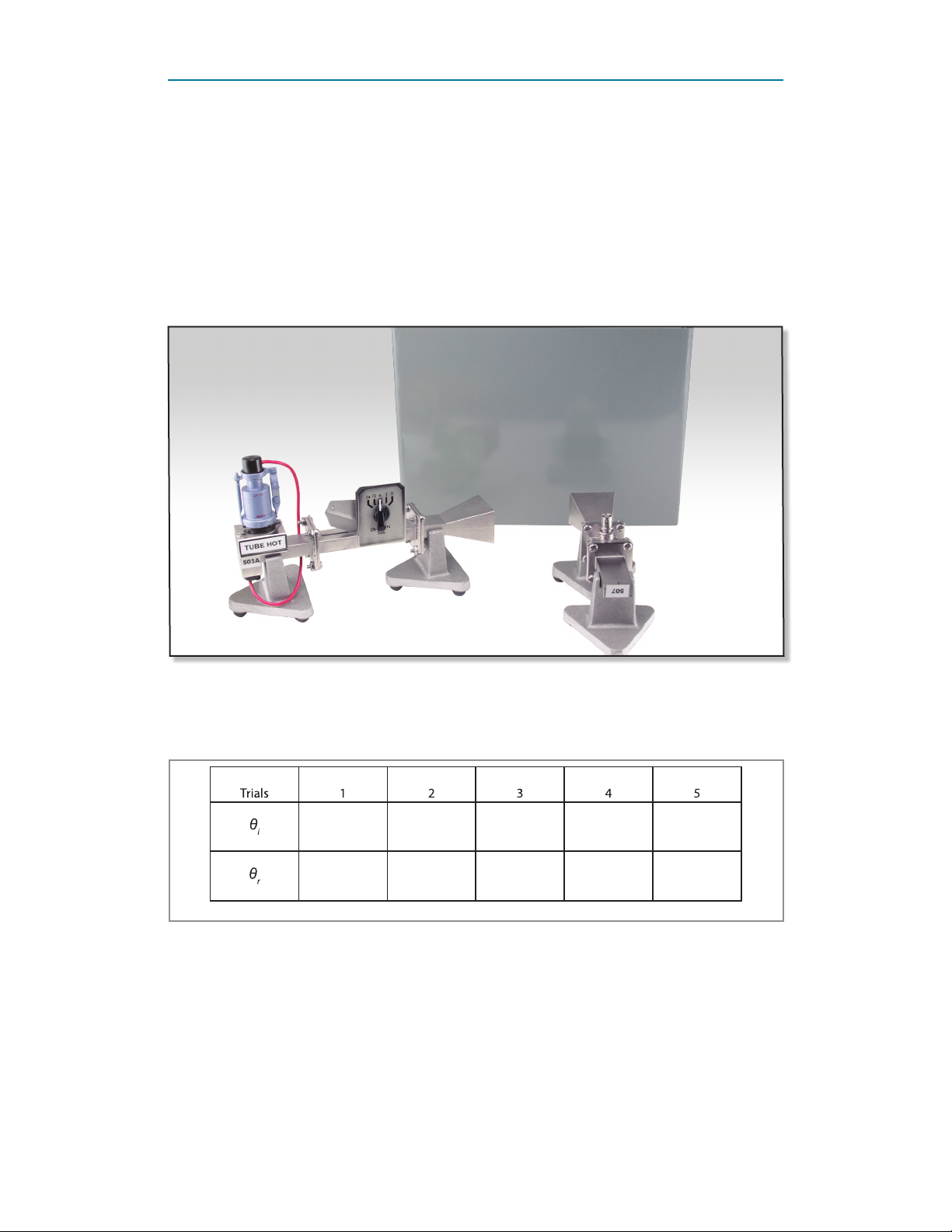
8. Repeat step 7 two more times recording the values in Table 4.1.
NOTE: Every time your pulse height drops in half, you have added about 3 dB
of attenuation to the line.
9. Set up Figure 4.5 so that the source and the receiver are facing at right angles to
one another and are about 1.5 times r
a part.
min
10. Find the spot (with the at reection) where the pulse height is maximum.
Table 4.2 Data
Trials 1 2 3 4 5
θ
i
θ
r
11. Record in Table 4.2 the angle θ
tenna.
12. Record in Table 4.2 the angle θ
antenna.
between the reector surface and the source an-
i
between the reector surface and the receiver
r
13. Repeat steps 10 through 12 at least ve times.
Microwaves for Everyone | LRL 550B Microwave Training Kit
41
Page 42
PriMArY MiCroWAVeS AntennAS – eXPeriMent 5
EXPERIMENT 5
Introduction
There are a number of types of primary antennas, such dipoles, horns, and polyrods, but
we will be discussing the horn antenna in this equipment.
Discussion
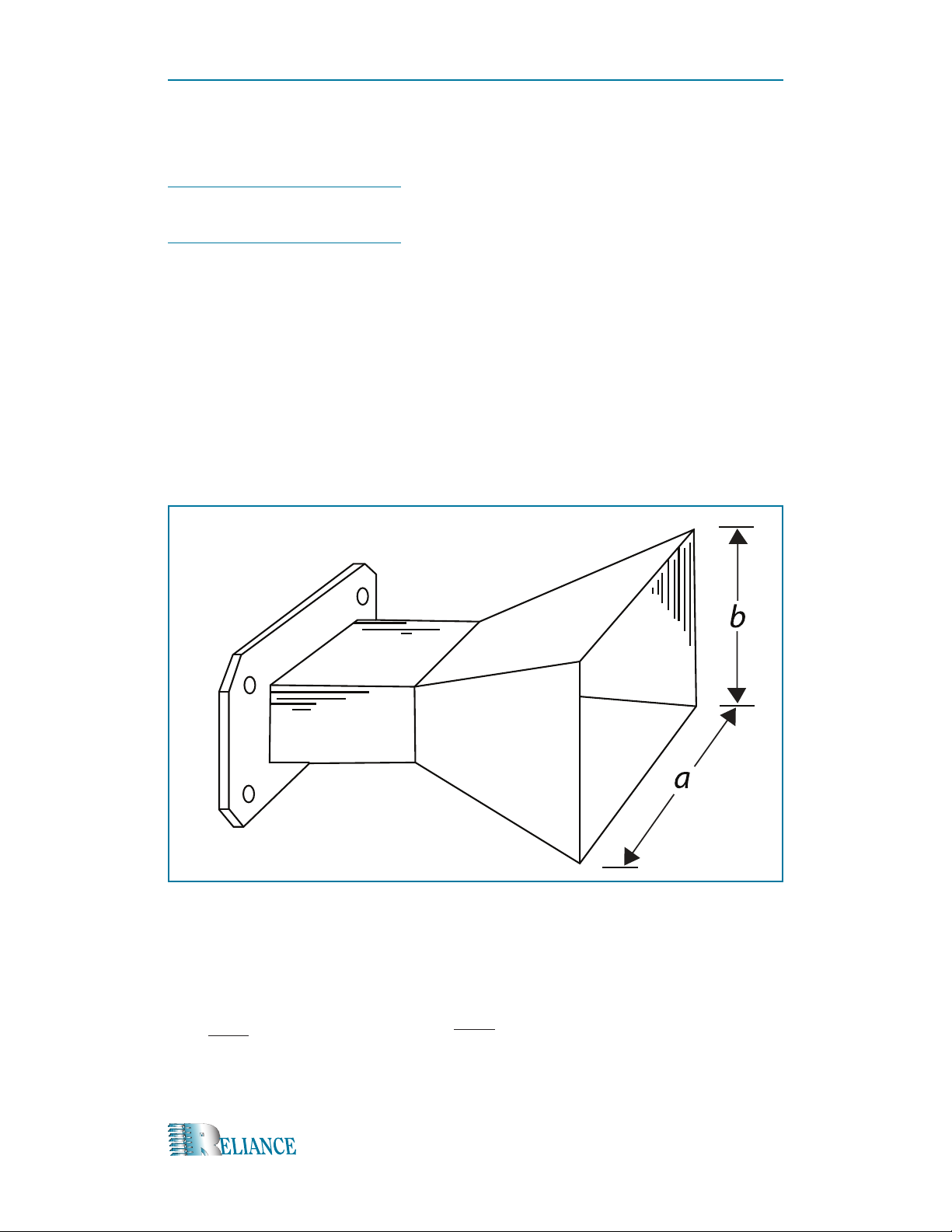
The microwave horn is a very simple antenna. It physically just tapers out from the
waveguide and has one job, to match the impedance of the waveguide to “free space”.
Horn antennas may be made several different ways. They can be tapered as “E” plane
horns, or “H” plane horns, but the antennas we will use is pyramidal or tapered in both
planes as in Figure 5.1.
42
Figure 5.1 Pyramidal Horn
Because the “H” plane and the “E” plane are not the same size, the resulting radiation
will not be the same width in both planes. They will be inversely proportional to the
dimensions of that plane. The widths are shown:
θ
80l
≈
H
0
a
and
Microwaves for Everyone | LRL 550B Microwave Training Kit
θ
53l
≈
E
0
b
Page 43

The gain of an antenna is the ratio of the surface area of a sphere with (radius) to the
actual area radiated by the antenna at range.
It is important that you understand that an antenna’s gain has nothing to do with the
power fed into it. The gain will be the same for a small signal or for a large one.
2pab
or
g =
2
l
0
When two horns are used together (one to transmit and one to receive), we can see the
transmitter gain and the receiver gain and separate them by a range. They give us:
g
r
rec
rec gtr l0
= r
( 4pr )
2
tr
But when the two horns are the same, we get:
2
2
g
l
r
= r
rec
0
( 4pr )
2
tr
Or:
4p
g = √r
r
l
0
rec
/ r
tr
When taking measurements in the laboratory, there are two main problems that must be
considered. One is the fact that measurements must be made with a minimum range is
no less than:
2
min
=
2d
l
0
r
Where d is the largest dimension of the transmitting antenna, the second problem is that
some of the transmitted power will be reected back up from the surface of the work
area. To prevent errors in this area, the minimum distance to surface should by no less
than:
l0 r
D
=
min
r is the range to the receiver and d the largest dimension of the transmitting horn.
2 d
Microwaves for Everyone | LRL 550B Microwave Training Kit
43
Page 44

PriMArY MiCroWAVeS AntennAS – eXPeriMent 5
PLEASE READ CAUTIONS CAREFULLY
BEFORE CONTINUING
CAUTION 1:
Klystrons get extremely hot when in use and must not
be handled while hot! Serious burns can result.
CAUTION 2:
Klystron mount, power supplies, and Klystron tube
plate caps have high voltages present when in use.
Exercise extreme CAUTION!
Shock or death can result.
CAUTION 3:
RF power levels in this kit are not harmful, but a
human eye may be damaged by low levels of
radiation.
Do not look into any waveguide at any time when
units are on.
44
Microwaves for Everyone | LRL 550B Microwave Training Kit
Page 45
Equipment and Components
• 1 RF microwave source (supplied- 510A).
• 1 Crystal detector (supplied- 518).
• 1 Waveguide termination (supplied- 507).
• 2 Waveguide horns (supplied- 531).
• 1 Cavity frequency meter (supplied- 504).
• 1 Variable attenuator (supplied- 506).
• 1 Oscilloscope (optional).
• 4 Waveguide stands (supplied- 523).
SEE CAUTION ON PREVIOUS PAGE
Objective
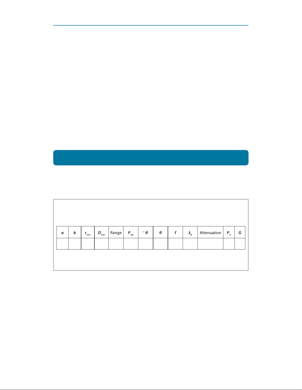
1. Measure and record the dimensions of one of the horns in Table 5.1.
a b r
min
D
min
Range P
2. Calculate the value of r
using l
min
Table 5.1 Data
1
θ θ f λ0Attenuation PtrG
2
rec
≈ 3cm.
0
Microwaves for Everyone | LRL 550B Microwave Training Kit
45
Page 46
PriMArY MiCroWAVeS AntennAS – eXPeriMent 5
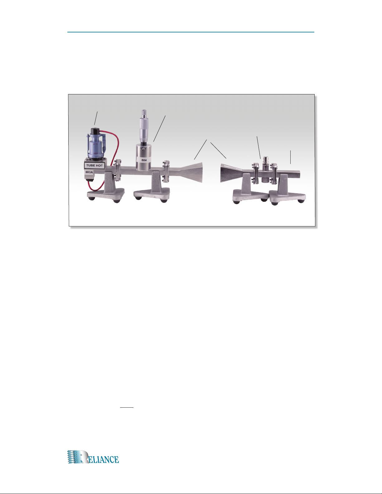
3. Set up Figure 5.2.
503A
504
531
518
507
4. Pick a good value of range greater than 2rmin (refer to discussion for the equation).
5. Position the receiving horn at the chosen range from the transmitter horn.
6. Set the attenuator for minimum, and turn on the source and allow it to warm up.
Record the pulse height Prec in Table 5.1.
7. Slowly rotate the receiver with respect to the transmitter until the pulse height
drops in half. Record the angle the receiver was turned.
46
8. The value in step 7 is one half the beam width of the antennas. Complete the total
beam width.
9. Return the test set up to the pulse height from step 6.
10. Measure the frequency with the cavity meter and calculate the transmitted
wavelength 20 .
11. Detune the cavity meter.
12. Remove the horns and connect the receiver directly to the attenuator.
13. Adjust the attenuator for a pulse height of step 6.
14. Record the attenuator setting. Calculate the pulse height that corresponds to the
transmitted power using the equation:
P
dB = 10 log
P
tr
rec
15. Calculate the gain of the antennas using data from step 6 and 14 (use equations
from the discussion).
Microwaves for Everyone | LRL 550B Microwave Training Kit
Page 47

Microwaves for Everyone | LRL 550B Microwave Training Kit
47
 Loading...