

LOUDSOFT Tutorial User Manual

Tutorial
www.loudsoft.com
In this tutorial we show several examples of simple and advanced X-over designs, using FINE Xover.
In the first example we create the x-over for two drivers we have previously measured in our
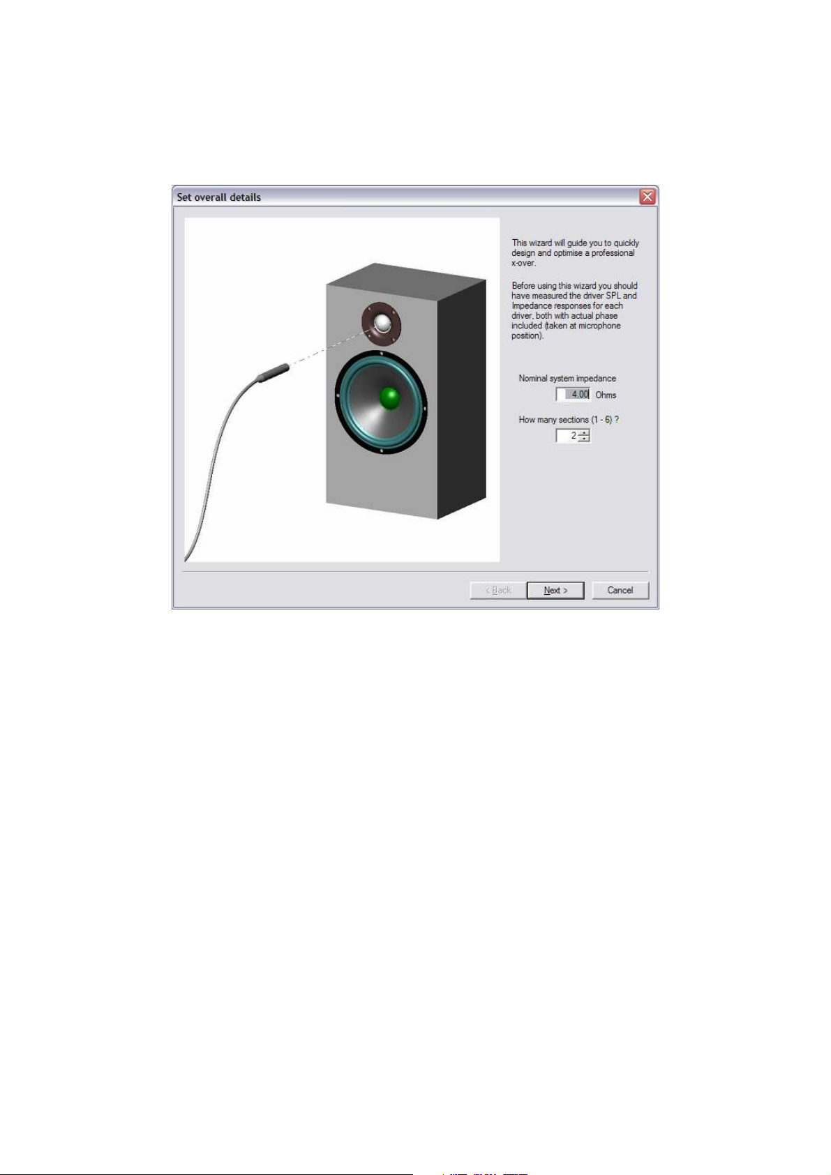
cabinet. Press New to get the Wizard, which will guide you to design the best possible x-over for
your system.
Figure 1. Wizard Start
We have the option to import measured files from FINELab (.lab) and FINECone (.FSIM) and a
number of systems like MLSSA, LMS, CALSOD, Sound-check etc. Here we use MLSSA files as
*.FRQ and *.TXT.
The two drivers are measured in the cabinet as shown on the sketch. We have placed the
microphone in the listening position (usually in line with the tweeter) and in the preferred 2-3m
distance. Then we have measured the woofer response and also exported as *.txt files (Actual +
BODE Plot in MLSSA). The tweeter is done the same way, with the microphone in the SAME
position. Finally we measured the impedance from 20-20kHz for both drivers
Choose the nominal system impedance, normally 4 or 8 ohms (mostly determined by the woofer)
even 1 ohm or 0.5 ohm is possible. This is used for initial x-over calculations and for minimum
impedance calculation. We will set the nominal impedance to 4 ohms (min impedance is therefore
4 ohms-20% =3.2 ohms). We choose 2 sections (2-way) as we have two drivers.
Press Next. Open SPL to load the file you had previously measured: SKO130-SPL.txt, and Open
Imp. to load the impedance file SKO130-Imp.FRQ, see Figure 3. You can click the file to preview
and check that you have selected the correct curve (Fig. 2).
Note the vertical line –––Target level. This is the level we want to optimise the system to. You can
drag the line up/down by the left mouse button, or overwrite the number (90.3 dB). We have
chosen the flat level above 200Hz for the woofer, because this is close to the maximum level we
expect to get out of the total system. We will consider off-axis SPL files later.
2
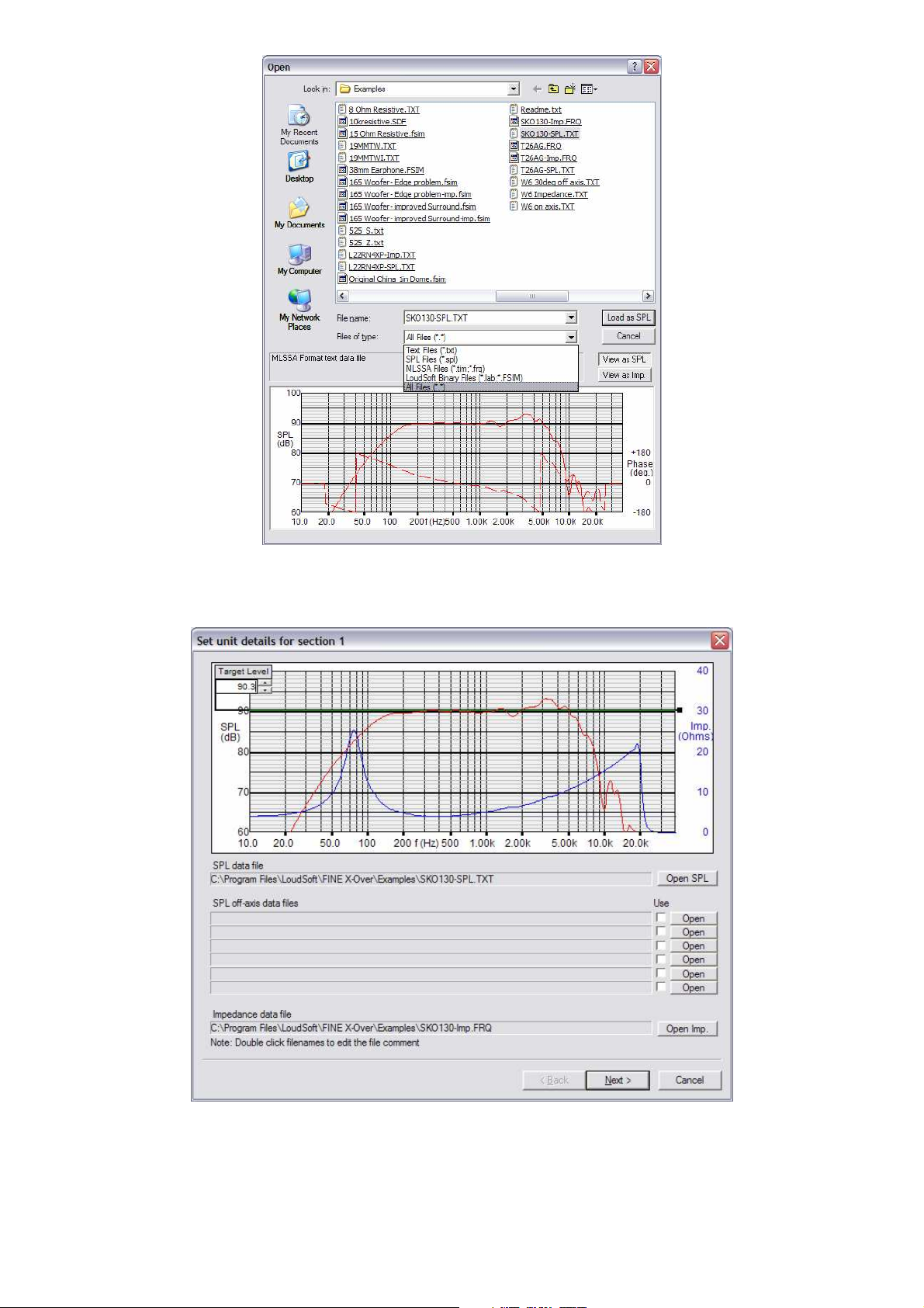
Figure 2. File Preview
Figure 3. File load
Press next to load the tweeter the same way. This time we use the measured T26AG.frq file
directly without exporting to txt-format. Let us keep the 90.3dB target level also for the tweeter.
3
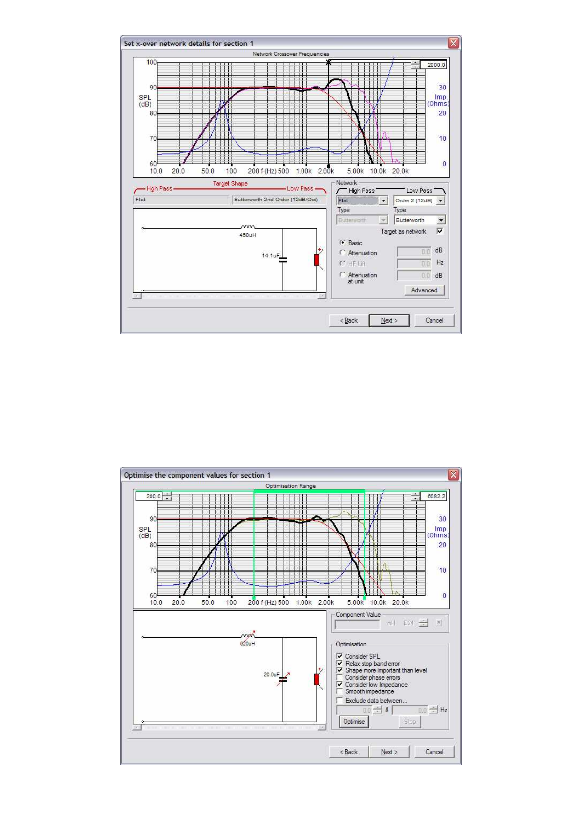
Figure 4. Target response
Now is the time to select the x-over type and Target frequency response. Figure 4 shows the first
section - woofer (LF). We may chose Butterworth (Linkwitz-Riley, Chebyshev and Bessel are also
possible) type and 1st Order (6dB/Oct) up to 4th Order (24dB/Oct). The black vertical x-line shows
the chosen x-over frequency, and we have selected 2nd order (12dB/Oct) Butterworth at 2000Hz.
You can drag the X-line by the left mouse button, while observing the filtered section response
change.
Figure 5. Optimise section 1
4
The next screen is the 1st (woofer) section Optimiser, Fig 5. Let us optimise the x-over
components to the target 2nd order Low Pass response (red–––––), while keeping a minimum
impedance of 4 ohms -20%=3.2 ohms (according to the common IEC 60268-5 standard). We
observe that the inductor (L) and capacitor (C) already are marked for optimisation, by the red
arrows.
The chosen optimising range is shown between the two green lines, which can be dragged as
before. It is important select the start at 200 Hz above the woofer resonance where the response
is almost flat (if the first green line is too low the optimisation gets bad). The upper limit is set by
default to two times the x-over frequency (=4000 Hz), which we drag to 6082.2 Hz to include the
top end.
Observe the Optimisation settings on the right side: “Consider SPL” and “Relax stop band error”
are selected by default. We could select “Shape more important than level” because that may help
the optimiser to find a good response at a higher SPL level. Further “Consider low impedance” is
set to avoid getting lower than minimum impedance.
Now we press “Optimise” and see the optimised response in a few seconds.
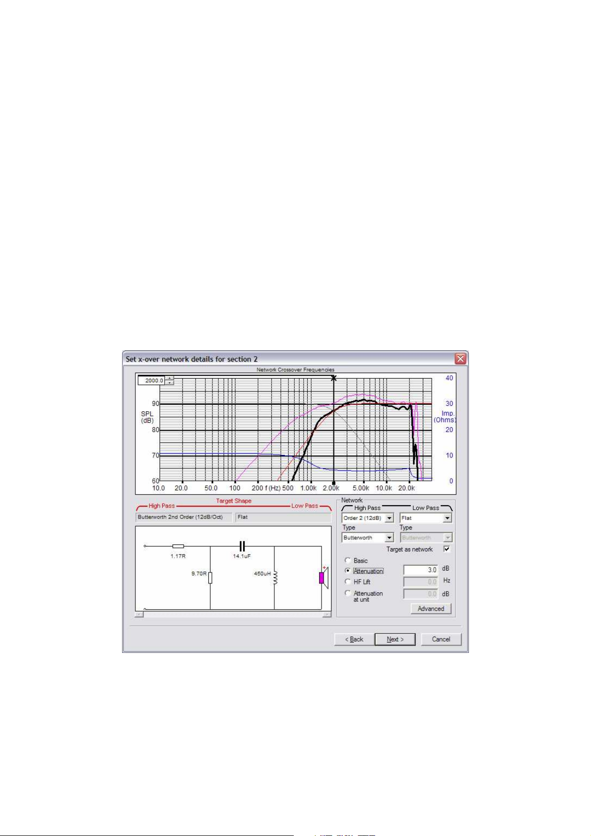
The next screen Fig. 6 shows the target response for the 2nd (tweeter) section with the already
chosen x-over frequency (2000 Hz) marked. We have chosen attenuation (3 dB by resistors),
because the tweeter sensitivity is above the target.
Figure 6. Target tweeter response
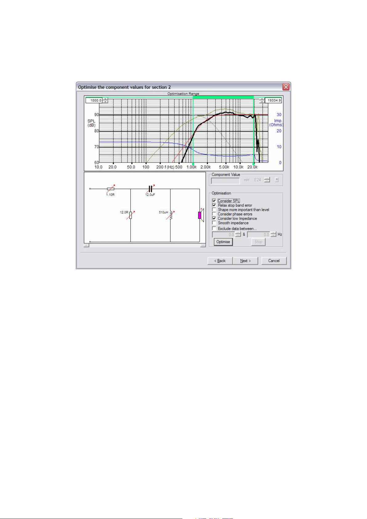
Fig. 7 shows the HF (Tweeter) optimising range is set from 1000 to almost 20 kHz, because we
want to include the top end response without exceeding the limit in the impedance response at 20
kHz,
If you want to keep any of the components as a fixed value, just double click and the red arrow
(=variable) is removed.
5
After pressing “Optimise” we see the optimised HF/ Tweeter response is quite close to the target.
The Wizard is now finished.
See the total response in the main window with the optimised sections. This response is quite flat
already, however we should use the System Optimisation to obtain an even better total response.
Figure 7. Optimised HF section
The optimisation range is set as the “flat” part of the total response. However we have deselected
“Shape more important than level” because we are interested in the absolute best and flattest
response.
The final optimised response in Fig. 8, is flat within +/-1.0 dB from 150-20kHz. The minimum
impedance is above the limit (3.2 ohms) 20-20kHz. The resistor of 1Mohm is redundant and can
safely be removed.
6

Figure 8. Final optimised response w. acoustical and Impedance Phase
The power in the woofer (LF) and tweeter (HF) is shown under the driver symbols with red
numbers, 17.4W and 1.32W respectively, for 50W RMS input (IEC 60268-1: Simulated Music).
Note you can always change component values by clicking (left mouse button), and you will get
the edit menu shown in the lower right corner. Change (standard E24/E12...) values by rolling the
mouse wheel up/down or use the arrow keys in menu or keyboard.
Press Total SPL Phase and Total Imp Phase to view the acoustical and electrical phase
responses, see Fig. 8. The acoustical phase (-----) is quite linear and the electrical phase (……) is
well behaved within +/- 45deg up to 20 kHz.
You may save the total response for later in user memory or as a file using the button bar:
7
 Loading...