

L DESIGN FEATURES
a
Z IP
2
0
2
2
=
DIPLEXER
ADC
ADC
0°
I/Q DEMOD
AGC
BAND
FILTER
LOWPASS
FILTERS
BASEBAND
AMPLIFIERS
LNARF AT
1920 MHz–1980 MHz
FROM Tx
2110 MHz–2170 MHz
LO AT
1920 MHz–1980 MHz
90°
LO
RF TONE POWER = P
S
RF PASSBAND
SINGLE TONE EXAMPLE MODULATED SIGNAL EXAMPLE
DOWNCONVERSION
LO
RF PASSBAND
DC DUE TO 2ND ORDER
DISTORTION = a2PSZ
0
0 Hz 0 Hz
BASEBAND PSEUDO-RANDOM POWER
DUE TO 2ND ORDER DISTORTION
= 3a
2
2
Z0P
S
2
RF SIGNAL POWER = P
S
Understanding IP2 and IP3 Issues
in Direct Conversion Receivers for
WCDMA Wide Area Basestations
Introduction
A direct conversion receiver architecture offers several advantages over the
traditional superheterodyne. It eases
the requirements for RF front end
bandpass filtering, as it is not susceptible to signals at the image frequency.
The RF bandpass filters need only
attenuate strong out-of-band signals
to prevent them from overloading
the front end. Also, direct conversion
eliminates the need for IF amplifiers
and bandpass filters. Instead, the RF
input signal is directly converted to
baseband, where amplification and
filtering are much less difficult. The
overall complexity and parts count of
the receiver are reduced as well.
Direct conversion does, however,
come with its own set of implementation issues. Since the receive LO
signal is at the same frequency as
the RF signal, it can easily radiate
from the receive antenna and violate
regulatory standards. Also, a thorough
understanding of the impact of the
IP2 and IP3 issues is required. These
parameters are critical to the overall
performance of the receiver and the key
component is the I/Q demodulator.
Unwanted baseband signals can be
generated by 2nd order nonlinearity of
the receiver. A tone at any frequency
entering the receiver gives rise to a DC
offset in the baseband circuits. Once
generated, straightforward elimination
of DC offset becomes very problematic.
That is because the frequency response
of the post-downconversion circuits
must often extend to DC. The 2nd order
nonlinearity of the receiver also allows
a modulated signal—even the desired
signal—to generate a pseudo-random
block of energy centered about DC.
direct conversion receivers are susceptible to such 2nd order mechanisms
regardless of the frequency of the
incoming signal. So minimizing the
10
Unlike superheterodyne receivers,
effect of finite 2nd order linearity is
critical.
effect of 3rd order distortion on a direct
conversion receiver. In this case, two
signals separated by an appropriate
frequency must enter the receiver in
order for unwanted products to appear
at the baseband frequencies.
Second Order Distortion (IP2)
The second order intercept point (IP2)
of a direct conversion receiver system
is a critical performance parameter. It
is a measure of second order non-linearity and helps quantify the receiver’s
susceptibility to single- and 2-tone
interfering signals. Let’s examine how
this nonlinearity affects sensitivity.
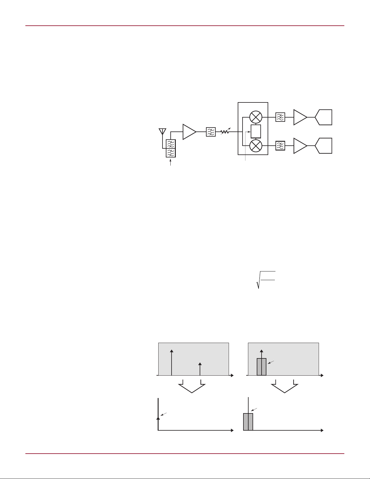
Figure 1. Direct conversion receiver architecture
Later in this article we consider the
Figure 2. Effects of 2nd order distortion
by Doug Stuetzle
We can model the transfer function
of any nonlinear element as a Taylor
series:
y(t) = x(t) + a2x2 (t) + a3x3(t) + …
where x(t) is the input signal consisting of both desired and undesired
signals. Consider only the second order
distortion term for this analysis. The
coefficient a2 is equal to
where IP2 is the single tone intercept
point in watts. Note that the 2-tone
IP2 is 6dB below the single-tone IP2.
The more linear the element, the
smaller a2 is.
Linear Technology Magazine • June 2008
DESIGN FEATURES L
P
Z
E A t t
S
=
{ }
1
0
2
• ( ) cos ω
P
Z
E A t E
t
S
= •
{ }
•
+
1 1 2
2
0
2
( )
cos ω
P
Z
E A t
S
=
{ }
1
2
0
2
• ( )
P
A
Z
S
=
2
0
2
E A t Z P
S20
2( )
{ }
=
y t A t t
a A t t
Higher Orde
( ) ( )cos
( ) cos
=
+
+…
ω
ω
2
2
rr Terms
A t t
a A t
a A t t
=
+
+
( ) cos
( )
( ) cosωω
1
2
1
2
2
2
2
2
2
……
DC OFFSET a A a P Z
S
= =
1
2
2
2
2 0
•
P
Z
E a A t
BB
=
1 1
2
0
2
2
2
• ( )
P
a
Z
E A t
BB
=
( )
{ }
2
2
0
4
4
• ( )
E A t E A t
4 2
2
3( ) • ( )
{ }
=
{ }
P
a
Z
E A t
BB
=
( )
{ }
3
4
2
2
0
2
2
• ( )
P a Z P
BB S
=
( ) ( )
3
220
2
y t A t t
a A t t B t t
u
( ) ( )cos
( ) cos ( ) cos
=
+ +
+
ω
ω ω
2
2
……
=
+ +
Higher Order Terms
A t t
a A t a
( ) cos
( )
ω
1
2
1
2
2
2
2
AA t t
a A t B t t t
A t
u
2
2
2
2
( ) cos
( ) ( )cos cos
( ) co
ω
ω ω+ …
= ss
( ) ( )cos( )
ω
ω ω
t
a A t B t t
u
+…
+ − …
2
ADC
0°
I/Q DEMOD
GAIN = 30dB
GAIN = 20dB
EQUIVALENT
PSEUDO-RANDOM
DISTORTION
AT –118.7dBm
TOTAL Rx
THERMAL NOISE
= –101.2dBm
WCDMA
INTERFERER
AT –40dBm
WCDMA
INTERFERER
AT –20dBm
DISTORTION
AT –98.2dBm
90°
Every signal entering the nonlinear
element generates a signal centered
at zero frequency. Even the desired
signal gives rise to distortion products
at baseband. To illustrate this, let the
input signal be represented by x(t) =
A(t)cosωt, which may be a tone or a
modulated signal. If it is a tone, then
A(t) is simply a constant. If it is a
modulated signal, then A(t) represents
the signal envelope.
By definition, the power of the desired signal is
where E{β} is the expected value of
β. Since A(t) and cosωt are statistically independent, we can expand
E{(A(t)cosωt)2} as E{A2(t)} • E{cos2ωt}.
By trigonometry
The expected value of the second
term is simply ½, so the power of the
desired signal simplifies to:
[1]
In the case of a tone, A(t) may be
replaced by A. The signal power is, as
expected, equal to
In the more general case, the desired signal is digitally modulated by
a pseudo-random data source. We
can represent it as bandlimited white
noise with a Gaussian probability
distribution. The signal envelope A(t)
is now a Gaussian random variable.
The expected value of the square of the
envelope can be expressed in terms of
the power of the desired signal as:
[2]
Now substitute x(t) into the Taylor
terms of the desired signal power, we
must relate E{A4(t)} to E{A2(t)}. For a
Gaussian random variable, the follow-
ing relation is true:
series expansion to find y(t), which is
the output of the nonlinear element:
expressed as
terms of the desired signal power:
Consider the 2nd order distortion
term ½a2[A(t)]2. This term appears
centered about DC, whereas the other
2nd order term appears near the 2nd
harmonic of the desired signal. Only
the term near DC is important here,
as the high frequency tone is rejected
by the baseband circuitry.
In the case where the signal is a
to DC, and any modulated signal into
a baseband signal that makes 2nd
order performance critical to direct
conversion receiver performance. Unlike other nonlinear mechanisms, the
signal frequency does not determine
where the distortion product falls.
tone, the 2nd order result is a DC
offset equal to:
nonlinear element give rise to a beat
note/term. Let
[3]
If the desired signal is modulated,
then the 2nd order result is a modulated baseband signal. The power of
x(t) = A(t)cosωt + B(t)cosωut,
where the first term is the desired
signal and the second term is an unwanted signal.
this term is
This can be expanded to:
[4]
In order to express this result in
[5]
The distortion power can then be
Now express the expected value in
[6]
It is the conversion of any given tone
Any two signals entering the
Linear Technology Magazine • June 2008
Figure 3. 2nd Order distortion due to WCDMA carrier
The second order distortion term of
interest is a2A(t)B(t)cos(ω– ωu)t. This
term describes the distortion product
centered about the difference frequency between the two input signals. In the
case of two unwanted tones entering
the element, the result includes a tone
at the difference frequency. If the two
11

!$#
)1$%-/$
'!).D"
'!).D"
%15)6!,%.4
03%5$/2!.$/-
$)34/24)/.
!4nD"M
4/4!,2X
4(%2-!,./)3%
nD"M
4X3)'.!,
!4nD"M
4X3)'.!,
!4nD"M
$)34/24)/.
!4nD"M
4X3)'.!,
!4nD"M
4X3)'.!,
!4D"M
L DESIGN FEATURES
unwanted signals are modulated, then
the resultant includes a modulated
signal centered about their difference
frequency.
We can apply these principles to a
direct conversion receiver example.
Figure 1 shows the block diagram of
a typical WCDMA basestation receiver.
Here are some key characteristics of
this example:
q
Basestation Type: FDD, Band I
q
Basestation Class: Wide Area
q
Number of carriers: 1
q
Receive band: 1920MHz to
1980MHz
q
Transmit band: 2110MHz to
2170MHz
The RF section of this receiver includes a diplexer, a bandpass filter, and
at least one Low Noise Amplifier (LNA).
The frequency selective elements are
used to attenuate out-of-band signals
and noise. The LNA(s) establishes
the noise figure of the receiver. The
I/Q demodulator converts the receive
signal to baseband.
In the examples illustrated below,
the characteristics of the LT5575
I/Q demodulator as representative
of a basestation class device of this
type. Lowpass filters and baseband
amplifiers bandlimit and increase the
signal level before it is passed to the
A/D converters. The diplexer and RF
bandpass filter serve as band filters
only; they do not offer any carrier
selectivity.
The second order linearity of the
LNA is much less important than that
of the demodulator. This is because
any LNA distortion due to a single
signal is be centered about DC and
rejected by the demodulator. If there
are two unwanted signals in the receive
band (1960MHz, for example), then a
second order product is generated by
the LNA at the difference frequency.
This signal is demodulated and appears as a baseband artifact at the
A/D converter. We need not address
this condition, however, because out of
band signals emerging from the front
end diplexer are not strong enough
to create distortion products of any
importance.
Consider first a single unmodulated
tone entering the receiver (see Figure
12
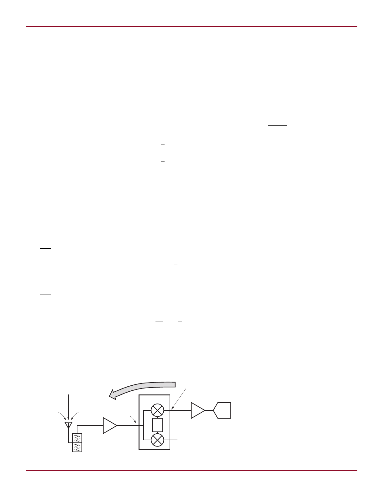
Figure 4. Transmitter leakage effects
2). As detailed above, this tone gives
rise to a DC offset at the output of the
demodulator. If the baseband cascade
following the demodulator is DC-coupled, this offset is applied to the A/D
predicts a distortion at the LT5575
output of –98.7dBm. This result agrees
well with that given by equation 6,
which predicts a distortion power of
–98.2dBm.
converter, reducing its dynamic range.
The WCDMA specification (3GPP TS
25104.740) calls out an out-of-band
tone at –15dBm, located 20MHz or
more from either receive band edge
(section 7.5.1). Compute the DC offset
generated in the I/Q demodulator:
q
Tone entering receive antenna
port: –15dBm
q
Diplexer rejection at 20MHz
offset: 0dB
q
Bandpass rejection at 20MHz
at the LT5575 output is a noiselike
signal, created from the interfering
WCDMA carrier. If this signal is large
enough, it can add to the thermal
receiver and A/D converter noise
to degrade sensitivity. Compute the
equivalent thermal noise at the receiv-
er input with no added distortion:
q
q
q
offset: 2dB
q
RF gain preceding LT5575: 20dB
q
Tone entering LT5575: 3dBm
q
LT5575 IIP2, 2-tone: 60dBm
q
LT5575 a2: 0.00317
q
DC offset at LT5575 output:
0.32mV
q
Baseband voltage gain: 31.6
q
DC offset at A/D input: 10mV
Single WCDMA carriers can also
serve as interferers, as detailed in
section 7.5.1. In one case, this carrier
is offset by at least 10MHz from the
desired carrier, but is still in the receive
band. The power level is –40dBm, and
the receiver must meet a sensitivity of
–115dBm for a 12.2kbps signal at a
BER of 0.1%. Here are the details:
q
Signal entering receive antenna
port: –40dBm
q
RF gain preceding LT5575: 20dB
q
Signal entering LT5575: –20dBm
q
LT5575 IIP2, 2-tone: 60dBm
q
LT5575 a2: 0.00317
A MATLAB simulation performed
using a pseudo-random channel
q
Now refer the distortion signal back
to the receiver input:
q
q
in this case is 17.5dB below the thermal noise at the receiver input. The
resulting degradation in sensitivity is
<0.1dB, so the receiver easily meets
the specification of –115dBm. This is
illustrated in Figure 3. Single WCDMA
carriers can also appear out of band,
as specified in section 7.5.1. These
can be directly adjacent to the receive
band at levels as high as –40dBm. Here
again, the second order effect of such
carriers upon sensitivity is negligible,
as the preceding analysis shows.
from transmitter leakage in FDD systems, as shown in Figure 4. In an FDD
system, the transmitter and receiver
The baseband product that appears
Sensitivity: –121dBm
Processing + coding gain: 25dB
Signal to noise ratio at sensitivity:
5.2dB
Thermal noise at receiver input:
–101.2dBm
RF gain preceding LT5575: 20dB
Equivalent interference level at
Rx input: –118.7dBm
The baseband second order product
Another threat to sensitivity comes
Linear Technology Magazine • June 2008

DESIGN FEATURES L
y t A t t
a A t t B t t
u
( ) ( )cos
( ) cos ( ) cos
= +…
+ +
ω
ω ω
3
33
3
2
3
+…
= +…
+
Higher Order Terms
A t t
a A t B
( ) cos
( ) (ωtt t t
a A t B t t t
A
u
u
)cos cos
( ) ( )cos cos
2
3
2 2
3
ω ω
ω ω+ …
= (( )cos
( ) ( )cos( )
t t
a A t B t t
u
ω
ω ω
+…
+ − …
3
4
2
3
2
P
Z
E a A t B t
BB
=
1 3
4
0
3
2
2
• ( ) ( )
P
a
Z
E A t E B t
BB
=
( )
{ } { }
9
16
3
2
0
2 4
• ( ) • ( )
P P P Z a
BB S u
=
( ) ( ) ( )
9
2
2
0
232
•
P a Z P P
BB S u
=
( ) ( ) ( )
27
2
3
2
0
2 2
•
ADC
0°
I/Q DEMOD
GAIN = 30dB
GAIN = 20dB
EQUIVALENT
PSEUDO-RANDOM
DISTORTION
AT –155.7dBm
TOTAL Rx
THERMAL NOISE
= –101.2dBm
WCDMA
INTERFERER
AT –48dBm
+ TONE AT
–48dBm
INTERFERERS
AT –28dBm
DISTORTION
AT –135.7dBm
90°
MODULATED SIGNAL AND TONE EXAMPLE
DOWNCONVERSION
LO
RF PASSBAND
0Hz
BASEBAND PSEUDO-RANDOM POWER
DUE TO 3RD ORDER DISTORTION
=9/2a
3
2
Z
0
2
PSP
u
2
RF SIGNAL
POWER = P
S
TONE
POWER = P
u
are operating at the same time. For
the WCDMA Band I case, the transmit
band is 130MHz above the receive
band. A single antenna is commonly
used, with the transmitter and receiver
joined by a diplexer. Here are some
typical basestation coupled resonator-type diplexer specifications:
q
Isolation, Tx to Rx 2110MHz:
55dB
q
Diplexer insertion loss, Tx path:
1.2dB
In the case of a Wide Area basestation, the transmit power may be as high
as 46dBm. At the transmit port of the
diplexer the power is at least 47dBm.
This high level modulated signal leaks
to the receiver input, and some portion
of it drives the I/Q demodulator:
q
Receiver input power: –8dBm
q
Rx BPF rejection at 2110MHz:
40dB
q
RF gain preceding LT5575: 20dB
q
Signal entering LT5575: –28dBm
q
LT5575 IIP2, 2-tone: 60dBm
q
LT5575 a2: 0.00317
A MATLAB simulation performed
using a pseudo-random channel predicts the following:
q
Distortion at LT5575 output:
–114.7dBm
Refer this signal back to the receiver
input:
q
RF gain preceding LT5575: 20dB
q
Equivalent interference level at
Rx input: –134.7dBm
q
Thermal noise at receiver input:
–101.2dBm
This equivalent interference is
33.5dB below the thermal noise at the
receiver input. The resulting degradation in sensitivity is <0.1dB, so the
receiver easily meets the specification
of –121dBm.
modulated signal, then B(t) represents
the signal envelope.
to y(t):
Figure 5. Effects of 3rd order distortion
Third Order Distortion (IP3)
The third order intercept point (IP3)
has an effect upon the baseband signal
when two properly spaced channels or
signals enter the nonlinear element.
Refer back to the transfer function:
y(t) = x(t) + a2x2(t) + a3x3(t) + …, where
x(t) is the input signal consisting of
both desired and undesired signals.
Consider now the third order distortion term. The coefficient a3 is equal
to 2/(3Z0IP3) where IP3 is the single
tone intercept point in Watts. Note
that the 2-tone IP3 is 4.78dB below
the single-tone IP3.
Two signals entering the nonlinear
element generate a signal centered
at zero frequency if the spacing between the two signals is equal to the
distance to zero frequency. Let x(t) =
A(t)cosωt + B(t)cosωut, where the first
term is the desired signal and the
second term is an unwanted signal.
The unwanted signal may be a tone
or a modulated signal. If it is a tone,
then B(t) is simply a constant. If it is a
terest here is ¾a3A(t)B2(t)cos(2ωu – ω)t.
In order for this distortion to appear
at baseband, set ω = 2ωu. The power
of the distortion is
which can be expanded to
desired signal and a tone interferer;
B(t) may be replaced by B. See Figure
5. The value of E{B4} can be expressed
as (2Z0Pu)2, where Pu is the power of
the tone interferer. We can use Equation 2 to express E{A
desired signal power as 2ZoPs, where
Ps is the power of the desired signal.
The power level of the distortion at
baseband is then:
The output signal is then equal
The third order distortion term of in-
[7]
Consider the case of a modulated
2
(t)} in terms of the
[8]
Linear Technology Magazine • June 2008
Figure 6. 3rd Order distortion due to WCDMA carrier + tone interferer
If the undesired signal is modulated,
use Equations 2 and 5 to express
E{B4(t)} as 3(2Z0Pu)2, where Pu is the
power of the tone interferer:
[9]
In the direct conversion receiver
example, Section 7.6.1 of the WCDMA
specification calls for two interfering
continued on page 27
13

DESIGN FEATURES L
1V/DIV
V
OUT3
V
OUT2
V
OUT4
V
OUT1
1ms/DIV
Authors can be contacted
at (408) 432-1900
can protect the rectifier diodes from
excessive reverse voltage and can
prevent pulse-skipping by limiting the
minimum duty cycle. Both of these
lockouts shut off all four regulators
when tripped.
These functions are realized with
a pair of built in comparators at
inputs UVLO and OVLO. A resistor
divider from the VINSW pin to each
comparator input sets the trip voltage
and hysteresis. The VINSW pin pulls
up to V
when any RUN pin is pulled
IN1
high, and is open when all three RUN
pins are low. This reduces shutdown
current by disconnecting the resistor
dividers from the input voltage. These
comparators have a 1.2V threshold
and also have 10µA of hysteresis.
The UVLO hysteresis is a current sink
while the OVLO hysteresis is a current
source. UVLO should be connected to
VINSW and OVLO connected to ground
if these functions aren’t used.
Frequency Control
The switching frequency is set by a
single resistor to the RT/SYNC pin.
The value is adjustable from 250kHz
to 2.5MHz. Higher frequencies allow
smaller inductors and capacitors, but
efficiency is lower and the supply has
a smaller allowable range of step-down
ratios due to the minimum on and off
time constraints.
The frequency can also be synchronized to an external clock by
connecting it to the RT/SYNC pin. The
clock source must supply a clock signal
whenever the LT3507 is powered up.
This leads to a dilemma if the clock
source is to be powered from one of the
LT3507 regulators: there is no clock
until the regulator comes up, but the
regulator won’t come up until there’s a
clock! This situation is easily overcome
with a capacitor, a low leakage diode
and a couple of resistors. The capacitor isolates the clock source from the
RT/SYNC pin until the power is up
and the resistor on the RT/SYNC pin
sets the initial clock frequency. The
application in Figure 1 shows how
this is done.
Typical Application
Figure 1 shows a typical LT3507 application. This application allows a
very wide input range, from 6V to 36V.
It generates four outputs: 5V, 3.3V,
2.5V and 1.8V. Efficiencies for three
of the outputs are shown in Figure 2.
The LDO produces a particularly low
noise output at 2.5V, as shown in
Figure 3.
The outputs are set to coincident
tracking using the 5V supply as the
Figure 4. Coincident tracking waveforms
master. But wait, there’s no resistor
divider on the TRK/SS4 pin! It’s no
mistake; the LDO output coincidently
tracks the supply it’s sourced from
(the 3.3V supply in this case) as long
as Q1 is a low V
transistor, such
CESAT
as the NSS30101 used here. Just
remember that this little cheat only
works for coincident tracking. Figure 4
shows the start-up waveforms of the
four outputs.
In this application, the clock is
synchronized to an external source
that is powered from the 3.3V output.
A capacitor isolates the clock until the
3.3V supply is good, and then passes
the clock signal to the RT/SYNC pin.
It should be noted that the LDO can
actually supply up to 0.5A as long as
I
OUT4
+ I
OUT2
≤ 1.5A.
Conclusion
The LT3507 provides a compact
solution for four power supplies. Its
tiny 5mm × 7mm QFN package includes three highly efficient switching
regulators and a low dropout linear
regulator. Just a few small inductors
and ceramic capacitors are needed to
create four high efficiency step-down
regulators. Plenty of options insure
that the LT3507 meets the needs of
a wide variety of multiple output applications.
L
LT5575, continued from page 13
signals as shown in Figure 6. One of
these is a –48dBm CW tone, and the
other is a –48dBm WCDMA carrier.
These are offset in frequency so that
the resulting 3rd order product appears centered about DC. Compute the
intermodulation product generated in
the I/Q demodulator:
q
RF gain preceding LT5575: 20dB
q
Signals entering LT5575: –28dBm
q
LT5575 IIP3, 2-tone: 22.6dBm
q
LT5575 a3: 0.0244
A MATLAB simulation performed
using a pseudo-random channel pre-
Linear Technology Magazine • June 2008
dicts distortion at LT5575 output of
–135.8dBm. This result agrees well
with the equation 8, which predicts a
distortion power of –135.7dBm.
Refer this signal back to the receiver
input:
q
RF gain preceding LT5575: 20dB
q
Equivalent interference level at
Rx input: –155.8dBm
q
Thermal noise at receiver input:
–101.2dBm
The equivalent interference in this
case is 54.6dB below the thermal noise
at the receiver input. The resulting
degradation in sensitivity is <0.1dB,
so the receiver easily meets the specification of –121dBm.
Conclusion
The calculations given here using the
LT5575 I/Q demodulator show that a
WCDMA wide area basestation receiver
can be successfully implemented using
a direct conversion architecture. The
high 2nd order linearity and input 1dB
compression point of the LT5575 are
critical to meeting the performance
requirements of such a design.
L
27
 Loading...