

Page 1
Leica T-Scan Collect
Reference Manual
Version 10.35
English
Page 2

1 Introduction
1.1 Purchase
Congratulations on the purchase of the Leica Geosystems T-Scan Collect software.
This manual contains instruction for setting up the product and operating it. Read carefully through
the User Manual before you use the product.
These are original instructions and part of the software. Keep for future reference and pass on to
subsequent holders/users of the hardware or software. This User Manual contains information
protected by copyright and subject to change without notice. No part of this User Manual may be
reproduced in any form without prior and written consent from Leica Geosystems AG.
Leica Geosystems shall not be responsible for technical or editorial errors or omissions.
© Leica Geosystems AG
1.2 Trademarks
Product Names are trademarks or registered trademarks of their respective owners.
1.3 Validity of this Manual
This manual applies to the Leica Geosystems T-Scan Collect software.
1.4 Feedback
Your feedback is important as we strive to improve the quality of our documentation. We request
you to make specific comments as to where you envisage scope for improvement. Please use the
following E-mail address to send your suggestions:
support.tracker@hexagon.com
1.5 Contact
Leica Geosystems AG
Metrology Division
Moenchmattweg 5
5035 Unterentfelden
Switzerland
Phone +41-62-737 67 67
Fax +41-62-723 07 34
www.leica-geosystems.com/metrology
Page 3

2 Contents
1 Introduction ........................................................................................................ 1
1.1 Purchase ................................................................................................ ....... 1
1.2 Trademarks ................................................................................................... 1
1.3 Validity of this Manual ................................................................................... 1
1.4 Feedback ...................................................................................................... 1
1.5 Contact .......................................................................................................... 1
2 Contents .............................................................................................................. 2
3 Revisions ............................................................................................................ 6
4 T-Scan Collect - Software – Introduction ......................................................... 7
4.1 Installation and Program Start ....................................................................... 7
4.2 Licensing ................................................................................................ ....... 7
5 Working with Viewers ........................................................................................ 8
5.1 3D Viewer ..................................................................................................... 8
5.2 Status Indicators ......................................................................................... 12
5.3 Additional Coordinate Axes ......................................................................... 13
5.4 Data Explorer ................................................................ .............................. 13
6 Customizing the User Interface ...................................................................... 20
7 Measurement .................................................................................................... 24
7.1 Selection of Measurement Mode ................................................................ 24
7.2 Measurement Settings ................................................................................ 24
7.2.1 General ................................................................................................ 25
7.2.2 Line Scanner ........................................................................................ 25
7.2.3 Surface Mode....................................................................................... 27
7.2.4 3D Point Mode ..................................................................................... 31
7.2.5 Static Polyline Mode ............................................................................ 32
7.2.6 Dynamic Polyline Mode ....................................................................... 34
7.3 Starting a Measurement .............................................................................. 34
7.3.1 Surface Mode....................................................................................... 34
7.3.2 3D Point Mode ..................................................................................... 35
7.3.3 Static Polyline Mode ............................................................................ 36
7.3.4 Dynamic Polyline Mode ....................................................................... 37
7.4 Stopping a Measurement ............................................................................ 38
8 Interactive Tools ............................................................................................... 39
8.1 Selection Mode ........................................................................................... 40
8.2 Interactive Clipping...................................................................................... 40
8.3 Check Accuracy .......................................................................................... 40
8.4 Cross Sections ............................................................................................ 43
8.5 Create Reference Points ............................................................................. 44
8.6 Fill Holes (Triangle Mesh) ........................................................................... 45
8.7 Create Bridges (Triangle Mesh) .................................................................. 46
Page 4

8.8 Smoothing (Triangle Mesh) ......................................................................... 47
8.9 Decimate Mesh (Triangle Mesh) ................................................................. 48
8.10 Sharpen Edges (Triangle Mesh) ................................................................. 49
8.11 Alignment Calibration .................................................................................. 49
9 Calibration ........................................................................................................ 50
9.1 Calibrate measurement range ..................................................................... 50
9.1.1 Preparation .......................................................................................... 50
9.1.2 Procedure ............................................................................................ 50
9.2 Alignment Calibration .................................................................................. 53
9.2.1 Requirements for an Alignment Sphere ............................................... 53
9.2.2 Measurement Strategy ......................................................................... 53
9.2.3 Step-by-Step Guide ............................................................................. 56
10 Working with Files ........................................................................................ 59
10.1 Create New Project ..................................................................................... 59
10.2 Open Existing Project .................................................................................. 59
10.3 Save Project ................................................................................................ 59
10.4 Save Project Under New Name .................................................................. 59
10.5 Import Data ................................................................................................. 59
10.5.1 Using the File Menu ............................................................................. 60
10.5.2 Using the Data Explorer ....................................................................... 60
10.5.3 Using Drag and Drop ........................................................................... 60
10.6 Export Data ................................................................................................. 60
10.6.1 Using the File Menu ............................................................................. 60
10.6.2 Using the Data Explorer ................................ ................................ ....... 61
11 Processing of Data Sets ............................................................................... 62
11.1 Transform Data ........................................................................................... 62
11.1.1 Transform ............................................................................................ 62
11.1.2 Transform to Nominal Points................................................................ 63
11.1.3 3 Planes Alignment .............................................................................. 69
11.1.4 3-2-1 Alignment .................................................................................... 72
11.1.5 Scale ................................ ................................ ................................ .... 76
11.1.6 Mirror ................................................................................................... 76
11.2 Optimize Data ............................................................................................. 76
11.2.1 Smoothing ............................................................................................ 76
11.2.2 Decimating ........................................................................................... 77
11.3 Matching ..................................................................................................... 77
11.3.1 Global Matching ................................................................................... 77
11.3.2 Tolerance Based Matching .................................................................. 82
11.4 Optimize Triangle Meshes .......................................................................... 85
11.4.1 Remove Unassociated Areas............................................................... 85
11.4.2 Remove Outliers .................................................................................. 86
11.4.3 Noise Reduction ................................................................................... 86
11.4.4 Curvature Based Decimation ............................................................... 87
11.4.5 Smoothing ............................................................................................ 87
11.5 Interactive Tools .......................................................................................... 87
Page 5

12 Post-Processing ........................................................................................... 88
13 Calculation of Feature Lines ........................................................................ 92
13.1 Calculation of Feature Lines ....................................................................... 93
13.2 Calculation of V-Lines ................................................................................. 95
13.3 Interactive Generation of Polylines.............................................................. 96
13.4 Processing of Polylines and Triangle Meshes ............................................. 97
13.5 3D Viewer Control ....................................................................................... 99
14 Service ......................................................................................................... 100
15 Tracking System ......................................................................................... 101
15.1 Initialize ..................................................................................................... 101
15.2 Disconnect/Connect .................................................................................. 101
15.3 Environmental Parameters ........................................................................ 101
15.4 Laser Control ............................................................................................ 102
15.5 Reflectors ................................ ................................ ................................ .. 102
15.6 Information ................................................................................................ 102
15.7 Go Birdbath ............................................................................................... 103
15.8 Go Zero Position ....................................................................................... 103
15.9 Move Station ............................................................................................. 103
15.9.1 Measuring the Pass Points ................................................................ 104
15.9.2 Selection of Pass Points .................................................................... 105
15.9.3 Moving the Station ............................................................................. 106
15.9.4 Measuring the Pass Points ................................................................ 106
15.9.5 Transformation Results ...................................................................... 107
15.9.6 Invoking Move Station again .............................................................. 108
15.10 Release Motors ..................................................................................... 109
16 Digitize ......................................................................................................... 110
16.1 Start .......................................................................................................... 110
16.2 Stop ........................................................................................................... 110
16.3 Information ................................................................................................ 110
17 Settings ....................................................................................................... 112
17.1 Cross Sections .......................................................................................... 112
17.2 Matching ................................................................................................... 113
17.3 3D Viewer ................................................................................................. 115
17.3.1 General Settings ................................................................................ 115
17.3.2 Lines .................................................................................................. 115
17.3.3 Surfaces ............................................................................................. 116
17.3.4 Other Settings .................................................................................... 117
17.4 Dynamic Camera ...................................................................................... 118
17.5 Coordinate Axes........................................................................................ 119
17.6 Accuracy Check ........................................................................................ 119
17.7 Measuring Mode ....................................................................................... 119
17.8 Measurement ................................................................ ............................ 120
17.9 Acoustic Feedback .................................................................................... 120
17.10 Materials ................................................................................................ 121
Page 6

17.11 Adjust Size Automatically ...................................................................... 122
17.12 Display Scanner .................................................................................... 122
17.13 Display T-Probe ..................................................................................... 123
17.14 Display T-Probe Coordinates ................................................................ 123
17.15 Keep On Top ......................................................................................... 124
18 Extras ........................................................................................................... 125
18.1 Execute Macro .......................................................................................... 125
19 Help .............................................................................................................. 126
19.1 About T-Scan Collect ................................................................................ 126
20 Appendix ..................................................................................................... 128
20.1 DCOM Configuration ................................................................................. 128
20.2 T-Scan Collect vs. T-Scan Interface .......................................................... 131
21 Index ............................................................................................................ 135
Page 7
3 Revisions
Rev.
Date
Changes
Author
Released
1.0
04/2001
FP
3.0
01/2003
Adjustments for version 3.0
FP
BK
4.0
10/2003
Adjustments for version 4.0
FP
MPo/AB
4.2
4/2004
Adjustments for version 4.2
FP
BK
5.0
12/2004
Adjustments for version 5.0
FP
5.01
5/2005
Adjustments for version 5.01
FP
6.0
4/2006
Adjustments for version 6.0
FP
SG/AB
7.0
7/2007
Adjustments for version 7.0
FP
BK/SG
8.0
5/2009
Adjustments for version 8.0
FP/FS
FS/BK
9.0
8/2010
Adjustments for version 9.0
FP/FS
10.11
10/2013
Adjustments for version 10.11
FP
10.2
9/2014
Adjustments for version 10.20
MBN
AFU
10.3
12/2014
Adjustments for version 10.30
BK/MBN
AFU
10.32
12/2015
Adjustments for version 10.32
BK/MBN
AFU
10.34
07/2016
Adjustments for version 10.34
BK
AFU
10.35
08/2017
Adjustments for version 10.35
BK
AFU
Page 8
4 T-Scan Collect - Software – Introduction
4.1 Installation and Program Start
Installation of T-Scan Collect
T-Scan Collect has been pre-installed on your system. If you want to install it again, please use the
Product USB Stick. Please note that T-Scan Collect is a 64-bit application and will only run on 64bit operating systems.
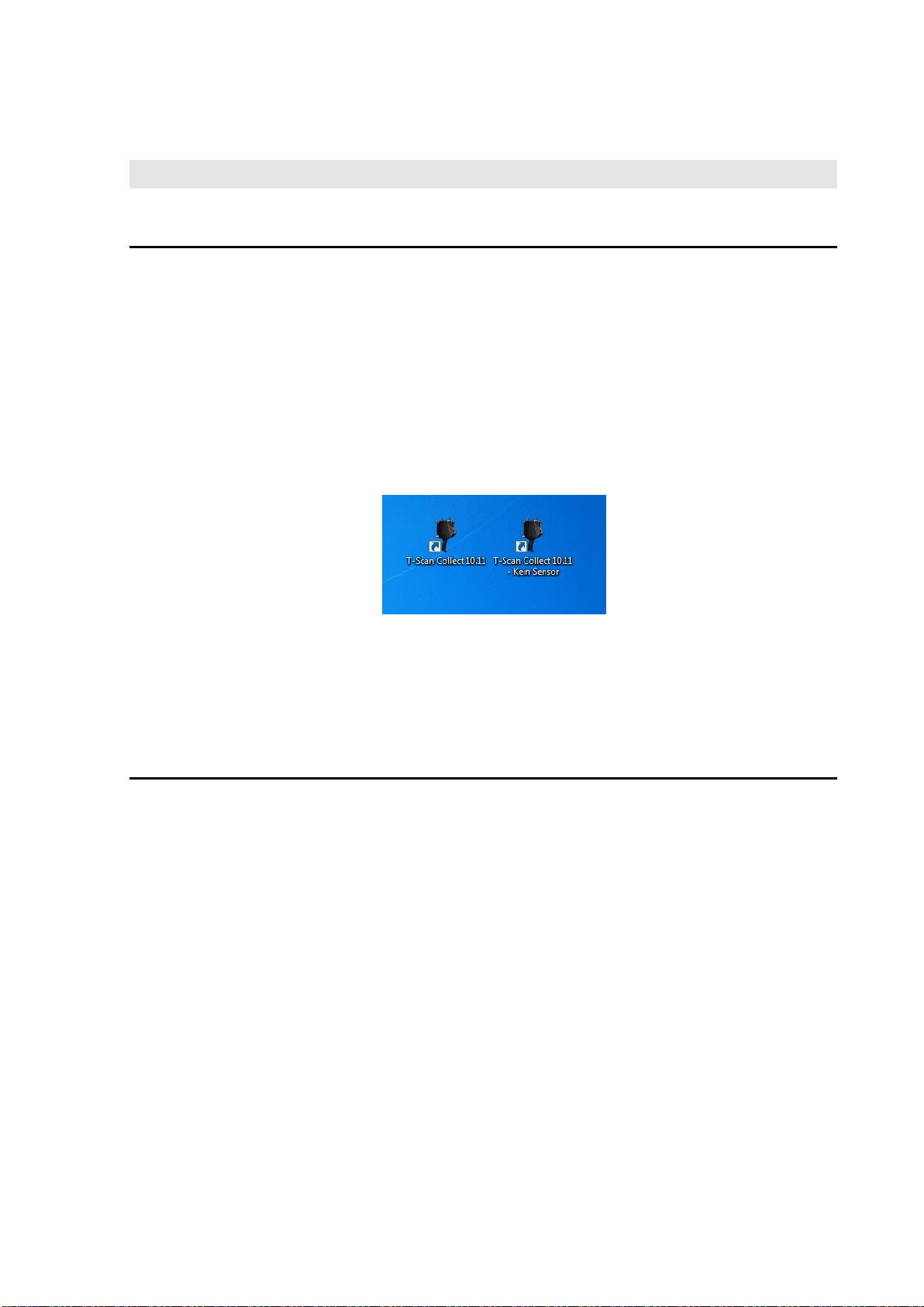
Start of T-Scan Collect
Use the Windows start menu or the shortcuts on your desktop to start the application.
If you only want to use T-Scan Collect for viewing, processing or evaluating data (i.e. you do not
want to measure), select the NoSensor shortcut which can be used without digitizing hardware.
4.2 Licensing
The T-Scan Collect software is protected by a CODEMeter dongle. The driver for the
CODEMeter dongle is automatically installed with the software. If you would like to upgrade
the software, please verify that the dongle is valid for the new software version. If you are
unsure, please contact support.tracker@hexagonmetrology.com and request the required
license file for upgrading the CODEMeter dongle to the new version. For more information, see
chapter 19.1.
Page 9
5 Working with Viewers
5.1 3D Viewer
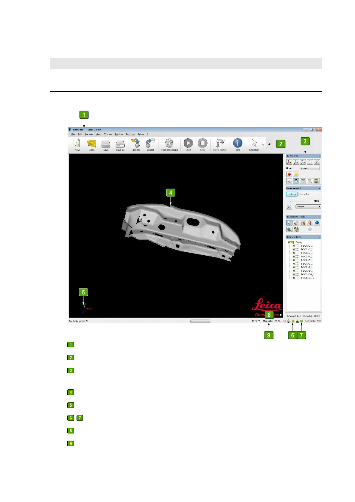
After the program start the user interface shows up:
Title bar, contains the name of current project
Toolbar with icons for frequently used functions
Several toolboxes. To save space, you can minimize/restore the toolboxes by clicking on the
corresponding button in their upper right corner
3D viewer with visualized data
Coordinate axes
, Status indicators for tracking system and controller, see chapter 5.2
Version information
Information from Weather Station
Page 10
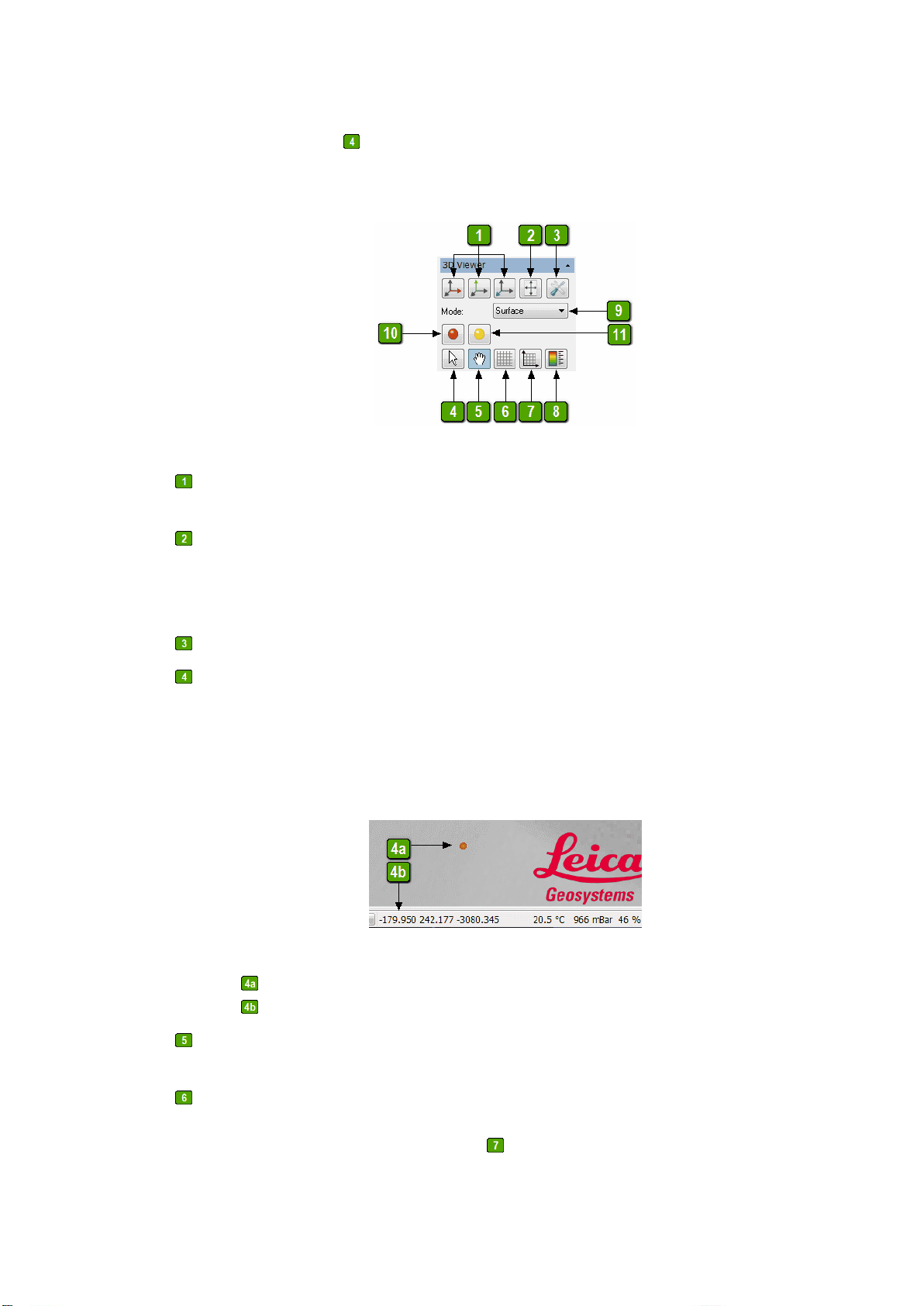
The area marked with in the above image shows the actual 3D viewer. The 3D Viewer
toolbox provides access to frequently used display functions:
Selection of viewing direction along the positive X, Y or Z coordinate axis. If you hold the
<Shift> key while clicking, the viewing direction is along the negative coordinate axis.
View all: If you use this button the zoom factor and the viewing position are adjusted so
that all visible data is shown. You can also achieve this by pressing the middle mouse button
while the cursor is over data or by holding down the <Shift> key and clicking with the left
mouse button in the 3D viewer.
Opens the dialog for the 3D Viewer Settings (see chapter 17.3).
Selection mode: By left clicking a data set in the 3D viewer, this data set is displayed in the
assigned selection color (see chapter 17.3.4) and marked red in the Data Explorer toolbox.
By right-clicking on a data point, the point is marked and its coordinates are displayed
(picking).
: Selected data point
: Point coordinates
Activation of viewing mode for interactive adjustment of the viewing direction, the position,
and the zoom factor.
Toggles a grid in the 3D viewer which can be used to quickly estimate distances or sizes. The
current distance between two major grid lines is displayed in the lower left corner. This
function cannot be used at the same time as .
Page 11
Show coodinate axes: This option is only available if the viewing direction is along a
coordinate axis (see ). The displayed coordinate axes are labeled. This function cannot be
used at the same time as . If you rotate the scene in the 3D viewer, the coordinate axis are
automatically hidden.
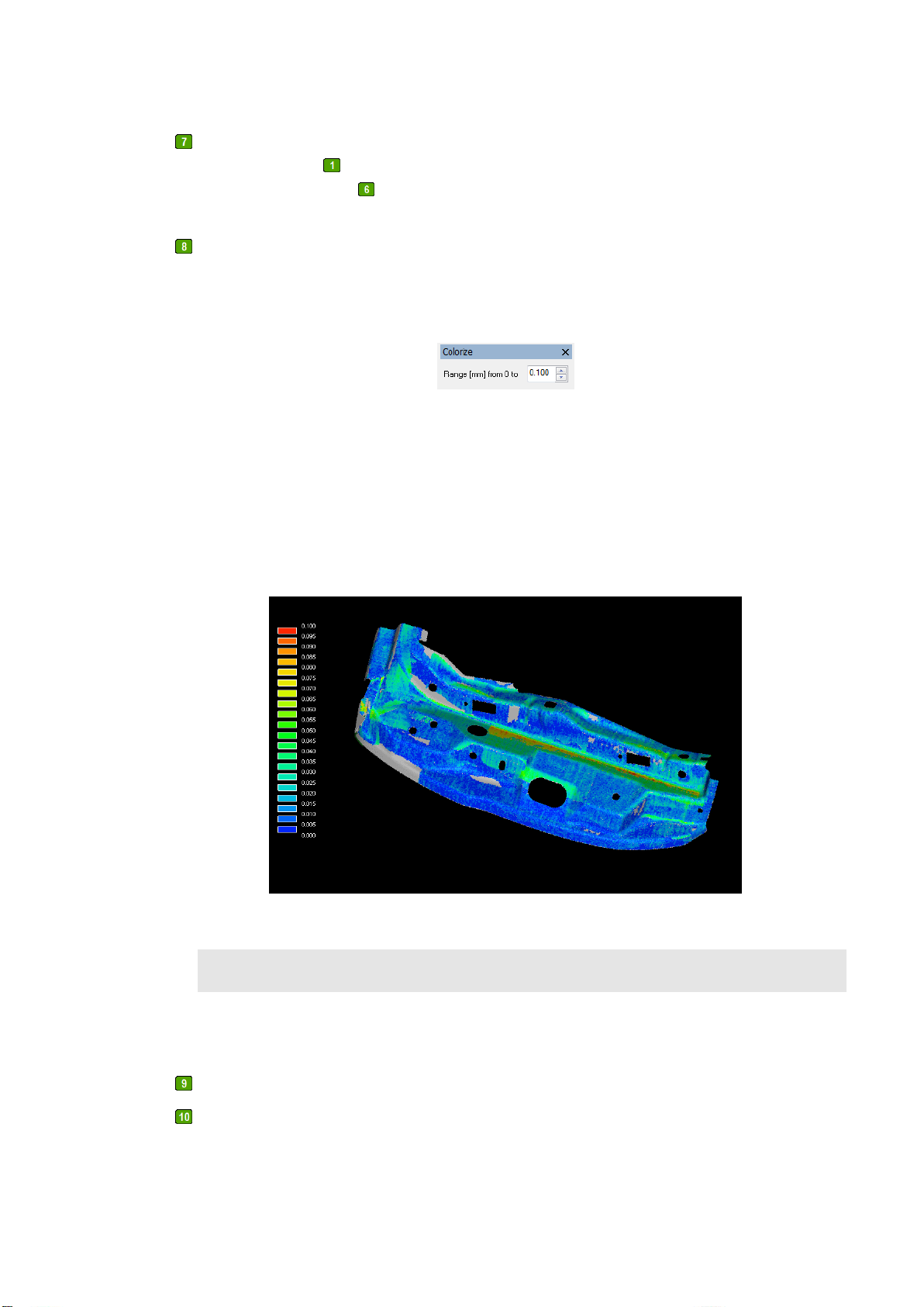
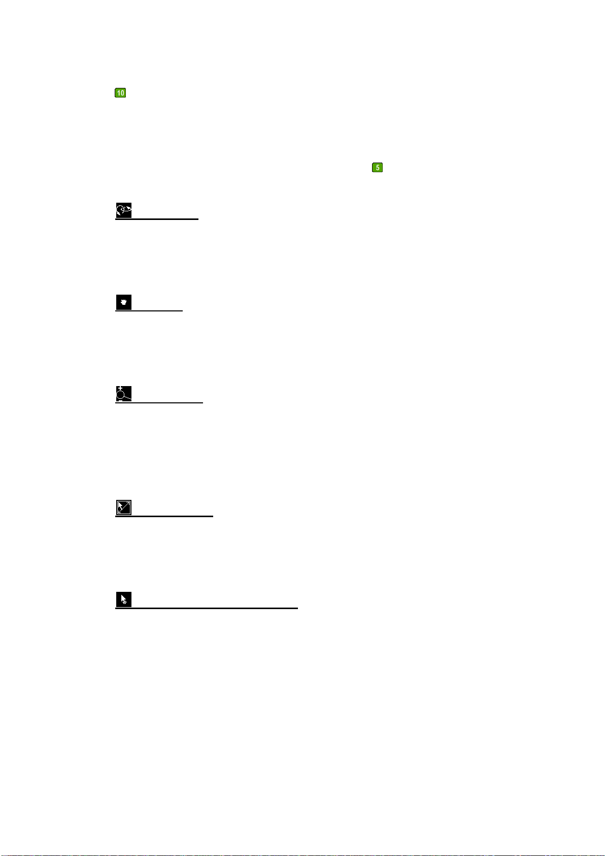
Colorize: This option is available as soon as two or more rasterized data sets are displayed.
When activated, overlapping areas of the data sets will be colorized according to the distance
of related points; a color lookup table indicates which color represents which distance.
The following toolbox opens:
Here you can enter the maximum distance that should still be colorized. This allows a quick
examination of the data quality and thus of the quality of the calibration. If large gaps occur
between the rasterized data, a tolerance-based matching (see chapter 11.3.2) or, if necessary,
a calibration (see chapter 9) should be performed. If deviations in data sets exceed the entered
value, they are displayed in the default color like scans that do not overlap.
Note
Colorizing large data sets may take a few seconds.
Viewing mode: The available settings are described in chapter 17.3.3.
Show/hide reference points: Toggles visualization of all nominal points created with the
Transform to Nominal Points wizard (see chapter 11.1.2).
Page 12
Show/hide tie points: Toggles visualization of all tie points created with the Move Station
wizard (see chapter 15.9).
The viewing direction, position and zoom factor in the 3D viewer can be interactively
controlled with the mouse. Activate the viewing mode or use <Space Bar> (as long as the
cursor is in the 3D viewer). In viewing mode, the following options are available:
Orientation:
Press the left mouse button, keep it pressed and move the cursor. The visualized object area is
shown using the dynamic display settings and is rotated according to the mouse movements.
When you release the left mouse button, the object is shown using the static displays settings
again.
Position:
Press the right mouse button, keep it pressed and move the cursor. The visualized object area
is shown using the dynamic display settings and is moved according to the mouse movements.
When you release the mouse button, the object is shown using the static display settings
again.
Zoom factor:
Press the middle mouse button, keep it pressed and move the cursor up and down. The
visualized object area is shown using the dynamic display settings and is zoomed according to
the mouse movements. When you release the mouse button, the object is shown using the
static display settings again.
You can also use the mouse wheel to change the zoom factor.
Zoom window:
Press the <Shift> key; the mouse cursor changes to an arrow with a rectangle. Press the left
mouse button while holding down the <Shift> key and move the cursor. As long as the left
mouse button is pressed, you can define a rectangular area. When you release the left mouse
button, the selected area is zoomed to fit the 3D viewer.
Defining the center of rotation:
To define the center of rotation, briefly press the <S> key. The cursor changes to an arrow with
a dot. With the left mouse button, click a point to define the center of rotation on the object’s
surface. The object is moved in such a way that the new center of rotation is in the center of
the 3D viewer.
Page 13
Note
Scanner: A symbol next to this graphic indicates whether a connection to the scanner
has been established.
If this symbol is green, a connection has been successfully established. If it is red, the
application has either been started in NoSensor mode or there is no connection to the
sensor via the controller. In this case, switch off the controller and check all connections
to the controller and to the sensor. Then switch the controller back on and wait until
the symbol turns green.
Tracking system: A symbol next to this graphic indicates whether a connection to the
tracking system has been established.
If this symbol is green, a connection has been successfully established. If it is red, the
application has either been started in NoSensor mode or there is no connection to the
tracker via the controller. In this case, switch off the controller and check all
connections to the controller and to the tracking system. Then switch the controller
back on and wait until the symbol turns green. The symbol for the tracking system is
yellow during measurement.
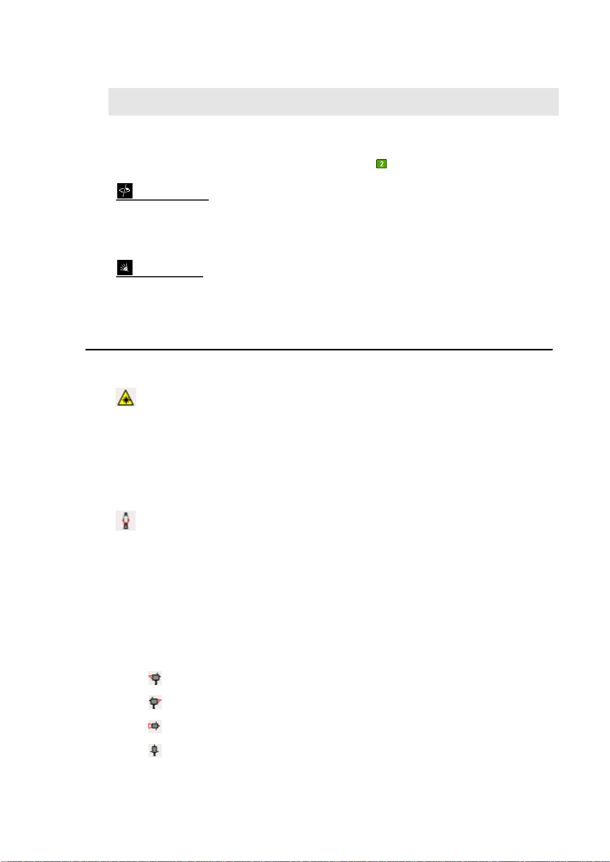
Probe: This icon show the probe that is currently tracked:
Scanner, left side (side 1)
Scanner, right side (side 4)
Scanner, top side (side 2)
Scanner, rear side (side 3)
By default, the center of rotation is in the center of gravity of the virtual box, which encloses
the whole object. However, you can freely determine the center of rotation as described above.
To set the center of rotation back to default, use the tool .
Axis rotation:
Press the <Alt> key and then press the left mouse button. Keep both pressed and move the
mouse cursor. A line from the center of rotation to the mouse cursor is drawn to help you
control the rotation. The view is rotated according to the mouse movements.
Illumination:
Press the <L> key and then press the left mouse button. Keep both pressed and move the
mouse cursor. The scene is illuminated according to the mouse movements.
5.2 Status Indicators
The status indicators are provided in the lower right area and can contain the following
symbols:
Page 14

T-Probe
Reflector
No Probe
Online Transformation: This symbol indicates that an online transformation is active
(see chapter 11.1.1).
5.3 Additional Coordinate Axes
By selecting Settings
arbitrary positions within the 3D viewer. The following dialog appears:
No additional coordinate axes
The additional axes will not be displayed.
Localize additional coordinate axes by picking
The positions of the additional coordinate axes can be defined by picking, as described in
chapter 5.1, item . The additional coordinate axes are positioned at the selected points.
Localize additional coordinate axes by selectable coordinates
The entries for the X, Y and Z coordinates contain the last defined positions of the coordinate
axes, regardless of whether they have been defined by picking or entered manually.
Coordinate axes, you can display additional coordinate axes at
New values take effect as soon as you click OK.
5.4 Data Explorer
This toolbox provides tools for grouping, editing and selecting data sets, and for the
customization of display characteristics.
Page 15
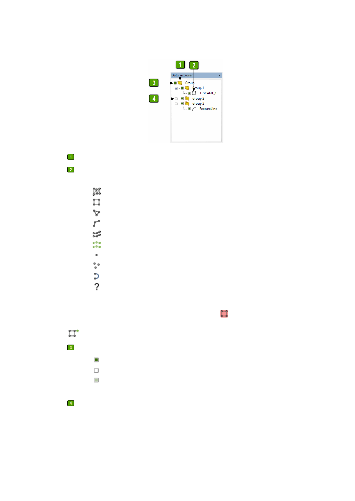
Group: The folder symbol represents a group, which may contain data or other groups.
Object name, data type and state: The object name is assigned automatically, but can be
changed. The symbol depends on the data type and can look like this:
Non-rasterized scan data
Rasterized scan data
Triangle mesh
Polyline
Polyline set
Alignment data
3D point
Unstructured point cloud
NURBS curve
Unknown data type
Symbols of selected data sets are highlighted in red, e.g. for a selected, rasterized data set.
If the data set is shown with customized display options, its symbol is marked with an asterisk:
.
Object visibility: This symbol can look like this:
for data: data is visible; for groups: all group entries are visible
for data: data is hidden; for groups: all group entries are hidden
only for groups: some group entries are visible, some are hidden
By clicking “+” or “-” you can expand or collapse groups.
When at least one object is selected in the data explorer, you can open a context menu with
the following commands by clicking the right mouse button:
Page 16
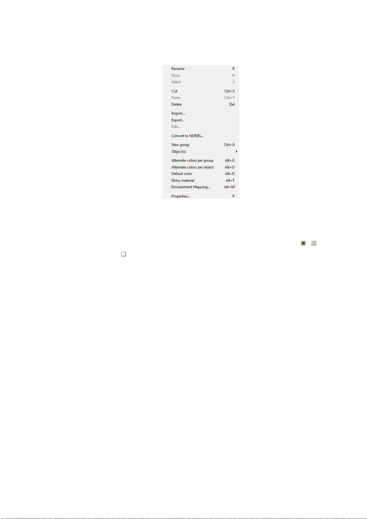
Rename
Renames the selected object. You can also achieve this by pressing <F2> or
clicking on the selected object.
Show / Hide
Shows or hides object(s). You can also achieve this by clicking the , and
symbols.
Select /
Deselect
Selects or deselects object(s)
Cut
Removes the selected objects and adds them to an internal clipboard
Paste
Adds objects from the internal clipboard to the selected group
Delete
Deletes the selected objects; this action cannot be undone!
Import
Imports data to the current group
Export
Exports selected data to a file
Edit
Only available for reference points; the following dialog appears:
Page 17
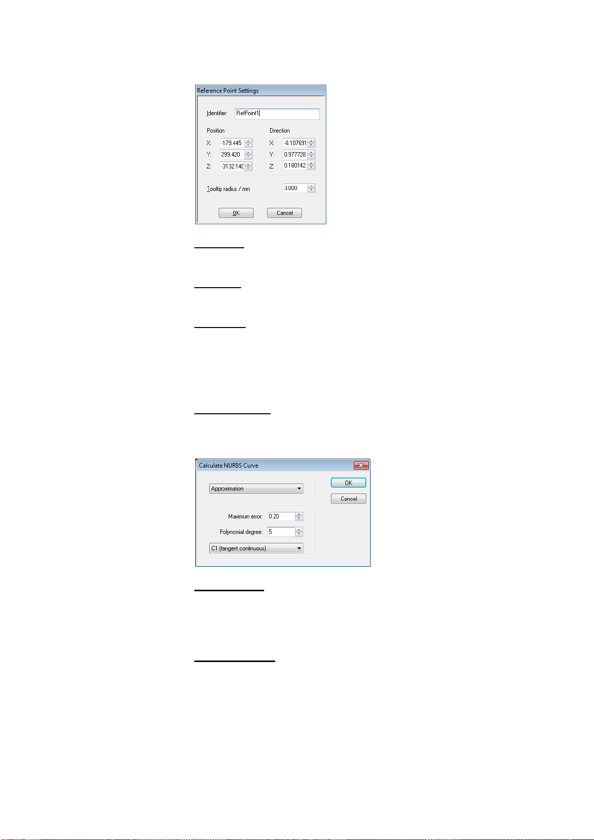
Identifier:
Displays the name of the reference point and allows renaming it
Position:
Displays the position of the current point
Direction:
If available: Direction from which the reference point was measured; the
length of the direction vector is normalized to 1 and the point is shown in
green. If no direction information is available, the fields display (0, 0, 0) and
the point is shown in blue.
Tooltip radius:
Displays the radius of the T-Probe’s tip with which the point was acquired.
Convert to
NURBS
Only applicable to lines; the following dialog appears:
Interpolation:
The NURBS curve passes exactly through the measurement points. By
adjusting the Polynomial degree and choosing the method, you can define
how the NURBS curve will be created.
Approximation:
The NURBS curve is approximated to the measurement points and will not
deviate by more than the specified maximum error at the control points. By
adjusting the Polynomial degree and choosing the method, you can define
how the NURBS curve will be created.
Three methods are available:
Page 18
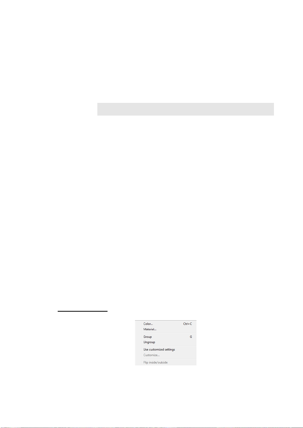
C0 (discontinuous): Neither the tangent nor the curvature of the created
NURBS curve will be continuous
C1 (tangent continuous): The tangent of the created NURBS curve will be
continuous
C2 (curvature continuous): The curvature of the created NURBS curve will
be continuous
Note
Depending on the data and the settings you choose it might happen that the
NURBS curve cannot be calculated. In this case, adjust the parameters and
recalculate the curve.
New group
Adds a new subgroup to the selected group
Object(s)
Opens the submenu for other object settings
Alternate
colors per
group
Assigns a different color to each group
Alternate
colors per
object
Assigns a different color to each object
Default color
Assigns the default color to each object
Shiny material
Assigns a shiny color and material to each object
Environment
Mapping
Opens a dialog where you can select an image that is projected onto the
objects and helps to identify faults in the surface. For best results select
Smooth shading in the 3D viewer settings.
Properties
Displays the characteristics of the object
Object(s) submenu:
Page 19
Color
Opens a dialog where you can choose a color for the selected objects
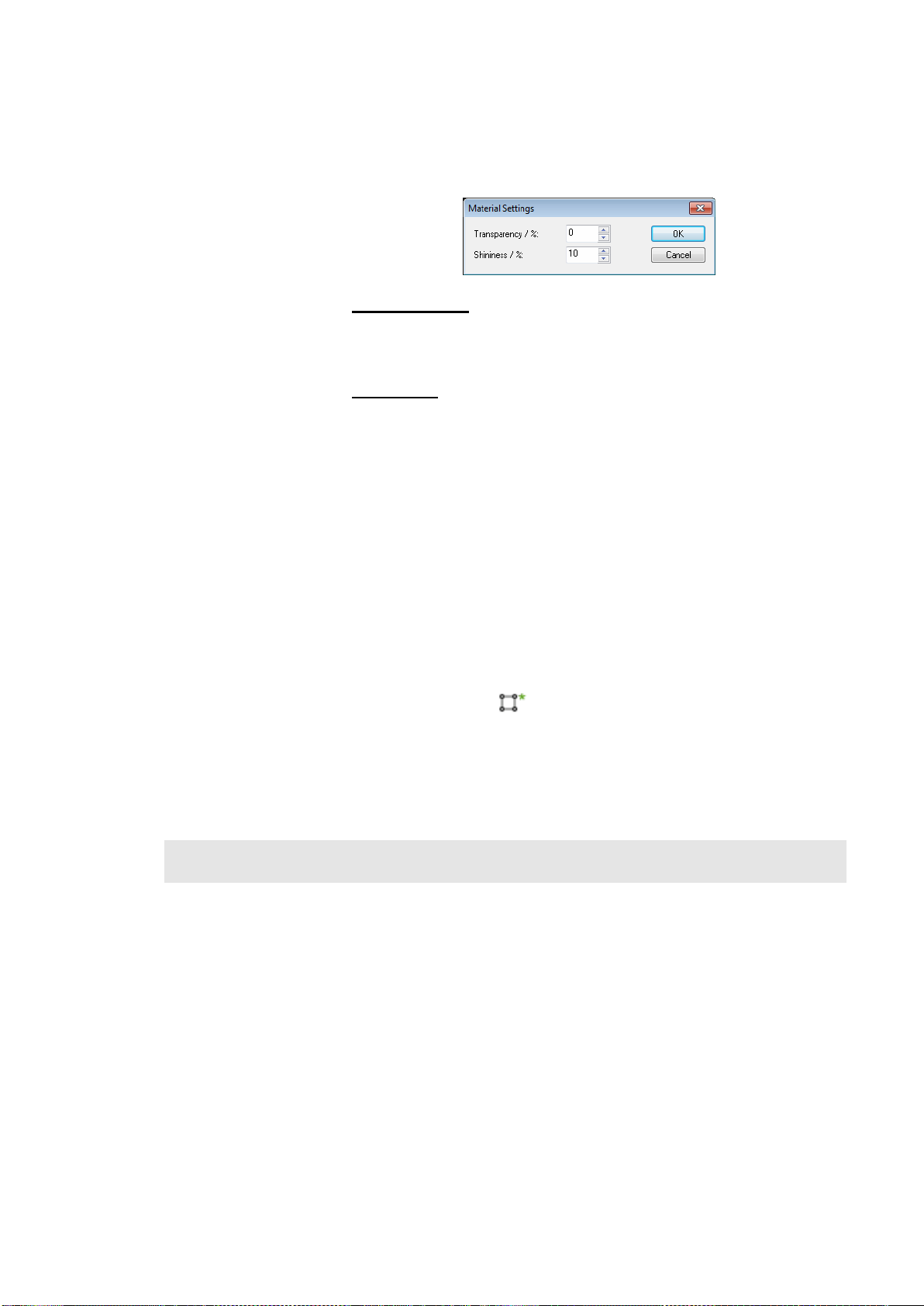
Material
The following dialog appears:
Transparency:
Enter the transparency of the object (in percent). 0% means the
object is opaque, 100% means it is translucent.
Shininess:
Enter the shininess of the object (in percent). 0% means the object is
not shiny, 100% means the object is very shiny.
Group
Combines all selected data sets (also those in a selected group) into a
new group. The name of the new group is the name of the first data
set in the group, followed by the number of data sets in the group (if
the group contains more than one data set).
Ungroup
Moves all selected data sets (also those in a selected group) to root
and then deletes all selected groups.
Use customized
settings
The selected objects are either displayed with the global settings for
the 3D viewer (see chapter 17.3) or with customized display settings.
The symbols of objects with customized display settings are marked
with an asterisk, e.g.: .
Customize
Opens a dialog for customizing the display settings for the selected
objects (see also chapter 17.3)
Flip inside/outside
Flips the inside and outside of a triangle mesh
Note
Please note that some commands are only available if a single object is selected, while other
commands are also available if multiple objects are selected.
You can select multiple objects in different ways:
1. Click the first object, then move the cursor to the last object. Press and hold the <Shift> key
2. Click the first object, then press and hold the <Ctrl> key and click other objects. Clicking an
and click the last object. All objects in-between are selected.
already selected object deselects it.
3. You can combine the two methods described above.
Page 20

4. You can also use the shortcuts <Shift> + <PageUp> / <PageDown> / <Home> / <End > to
select multiple objects.
Please keep in mind that any changes you make are also saved in the project. The next time you
open the project, all settings that were in effect the last time you saved the project will be
active again.
Shortcuts, cursor keys and drag and drop are easy ways to increase efficiency. When using
shortcuts, make sure that the data explorer has the focus.
Page 21
6 Customizing the User Interface
The T-Scan Collect user interface can be customized. You can define your own shortcuts,
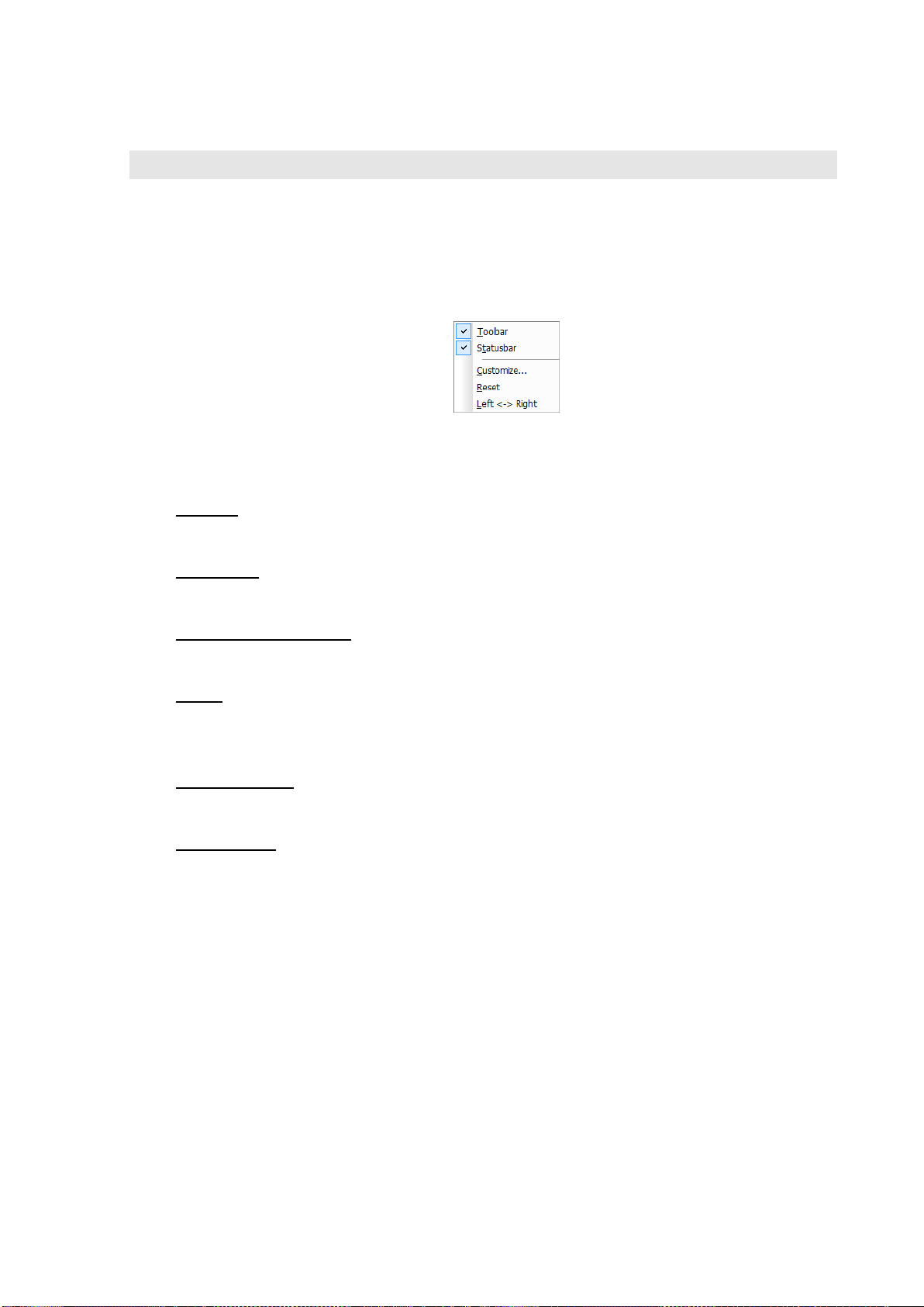
menus and toolbars. Choose View Toolbars or right-click a toolbar to open the context
menu.
The context menu provides the following functions:
Toolbar
Shows or hides the standard toolbar
Status bar
Shows or hides the status bar
User defined toolbars
If you defined your own toolbars, you can choose which to show or hide
Reset
Resets all shortcuts, menus and toolbars to the default settings of T-Scan Collect. All userdefined changes will be lost. This action cannot be undone!
Left Right
Swaps the positions of the toolbars
Customize...
Opens a dialog where you can define and change shortcuts, menus and toolbars. As soon as
the dialog is open, you can drag and drop buttons onto or off toolbars to move, add or delete
buttons.
The dialog contains various tabs:
Page 22
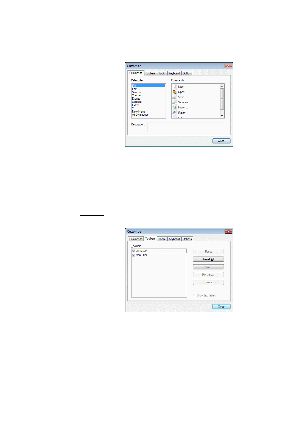
Commands
You can add all listed commands to a toolbar. Left-click a command and drag it onto a
toolbar while holding the mouse button down. When you release the mouse button,
the command is added to the toolbar.
You can also remove a command from a toolbar: Click the icon and drag it off the
toolbar while holding the left mouse button down.
Toolbars
A list shows the available toolbars. By selecting or deselecting the checkboxes in the
list, you can show or hide the toolbars.
To create a new toolbar, click New.... A dialog box appears where you can enter a
name for the new toolbar.
To delete a toolbar, select it and click Delete.
Page 23
Click Rename… to rename the selected toolbar. A dialog box appears where you can
enter a new name for the toolbar.
You can reset the standard toolbar to the default settings of T-Scan Collect by clicking
Reset. This action cannot be undone!
To reset all toolbars to the default settings of T-Scan Collect, click Reset All; userdefined toolbars will be lost. This action cannot be undone!
You can choose whether to show or hide the text labels of the icons by selecting or
deselecting the Show text labels checkbox.
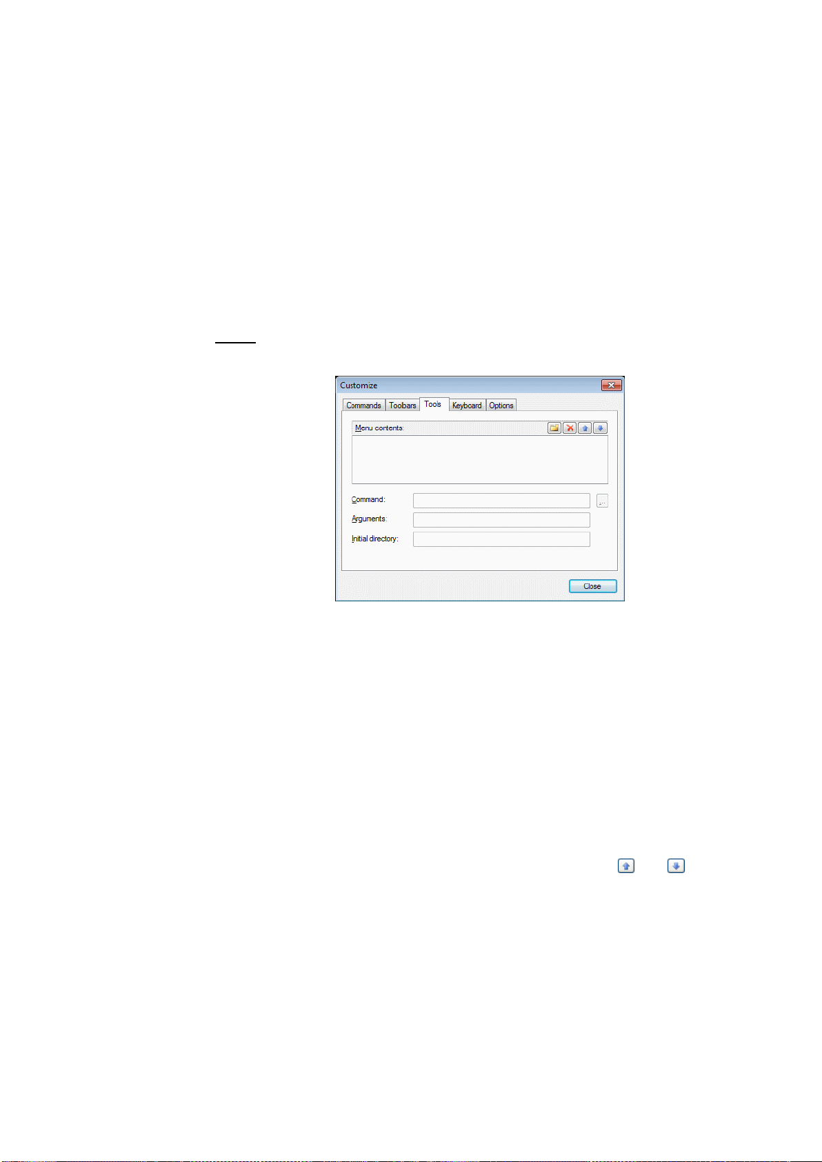
Tools
With this tab, you can manage the commands provided in the Extras menu.
By pressing the <Ins> key or clicking the New icon, you can create a new menu entry.
An input line appears where you can enter a name for the menu entry, e. g. “Start
COMET Inspect”. In the Command line, define the application that will be started
when the entry is selected; e. g. D:\Program Files\Steinbichler\INSPECTplus 5.23\
INSPECTplus.exe. If you want to pass arguments to the application, enter those in the
Arguments line. Initial Directory defines the directory in which the command will be
executed.
By pressing <Del> or clicking the Delete icon, you can delete the selected entry.
By pressing <Alt> and <Up> or <Alt> and <Down> or the icons and , you can
change the position of the selected entry within the menu.
Page 24
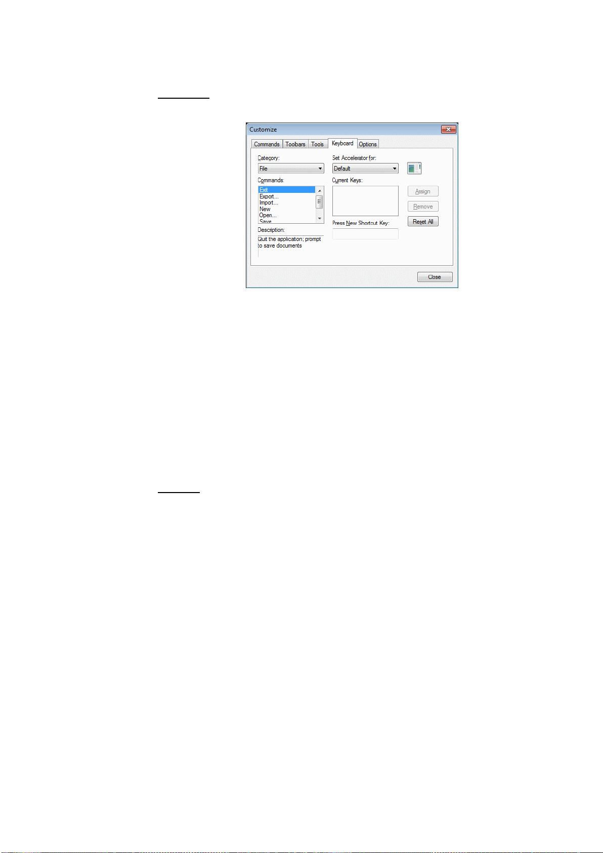
Keyboard
Here you can define shortcuts for all menu commands. In the Category list, select the
menu that contains the command. The Commands list then shows all the
commands of this category. Select the command for which you want to change the
shortcut. The current shortcut (if available) is displayed in the Current Keys box.
Select the input line for Press New Shortcut Key and press the key combination for
the new shortcut. Then click Assign.
To remove the shortcut for a command, select the command and click Remove.
To reset all shortcuts to the default settings of T-Scan Collect, click Reset All. This
action cannot be undone!
Options
Select or deselect Show ScreenTips on toolbars and Show Shortcut keys in
ScreenTips according to your preferences. It is recommended to select both options.
The Large Icons function is currently not supported.
Page 25
7 Measurement
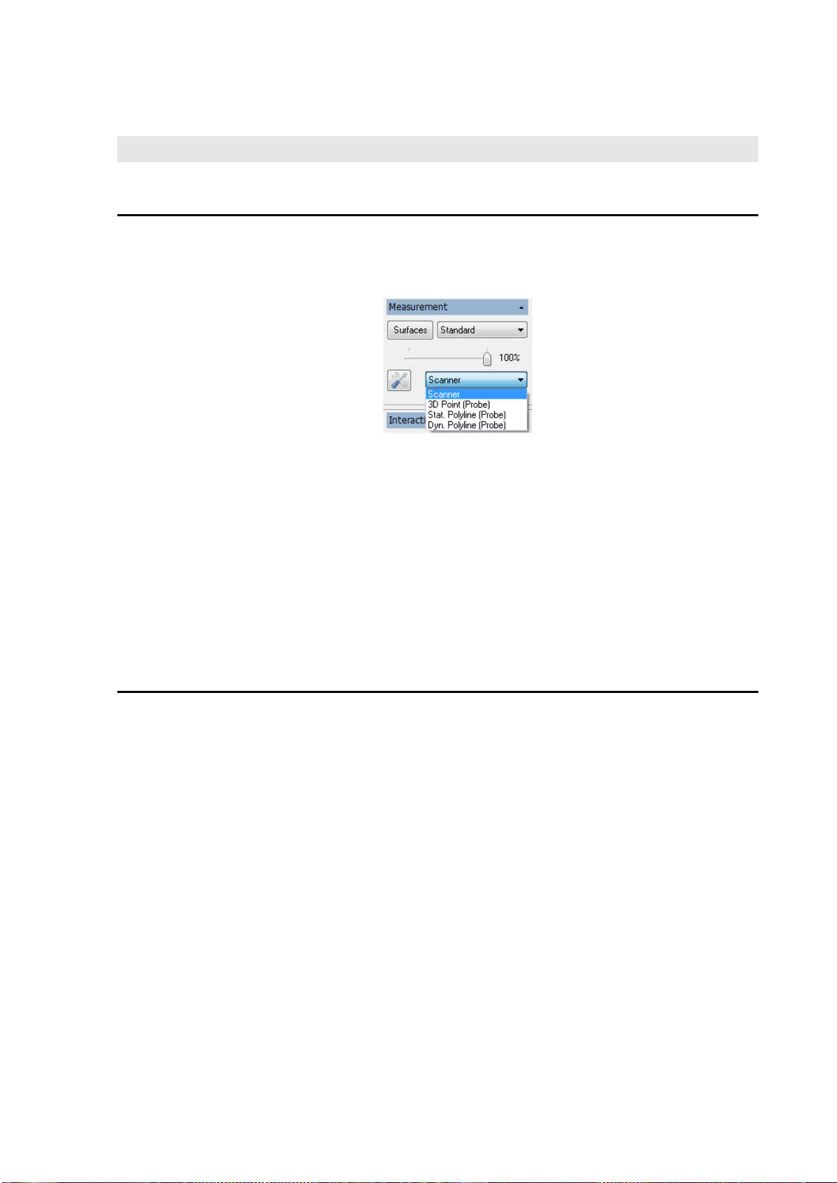
7.1 Selection of Measurement Mode
To select a measurement mode, choose Settings Measurement… or use the Measurement
toolbox:
In Surface mode, object surfaces can be digitized. This mode is activated after the
program start by default
In 3D Point mode, single points will be measured with the T-Probe (Probe)
In Static Polyline mode, lines will be measured with the T-Probe (Probe) where each point
of the line has to be measured explicitly
In Dynamic Polyline mode, lines are measured with the T-Probe (Probe) where the points
of the line will be measured automatically according to the chosen settings
7.2 Measurement Settings
The settings can be adjusted separately for almost every measurement mode. To do this,
choose Settings Measurement…. A dialog appears where you can select the tab for the
measurement mode you want to adjust. You can also open the dialog from the measurement
toolbox by clicking the Measurement parameter settings icon.
Page 26
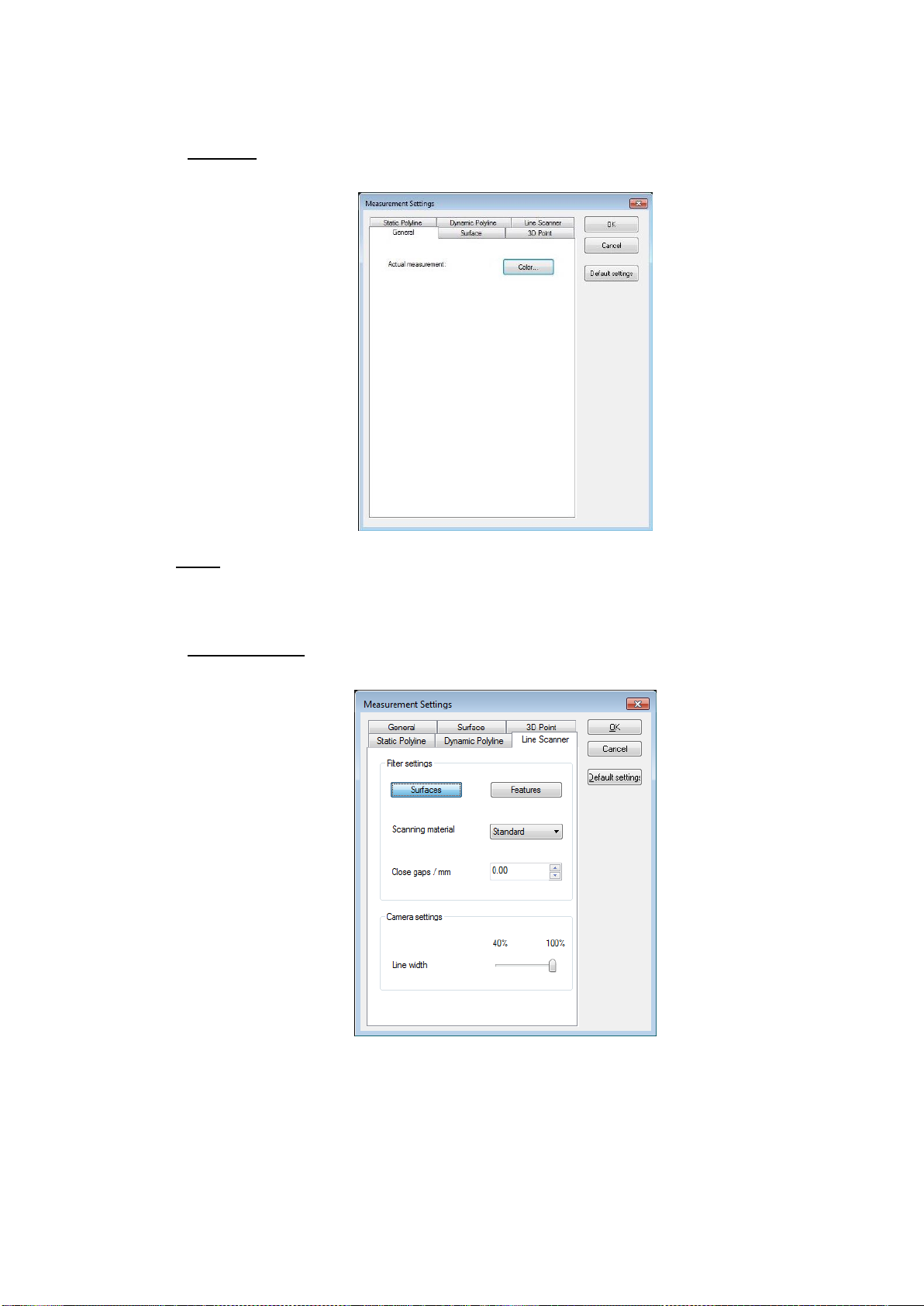
7.2.1 General
Color
This button opens a dialog where you can specify a color for the last measurement data you
acquired.
7.2.2 Line Scanner
This dialog provides settings for adjusting the line scanner. If inappropriate settings are made
here, however, you might not be able to acquire any measurement data. If you would like to
restore the default values, click the Default Settings button.
Page 27
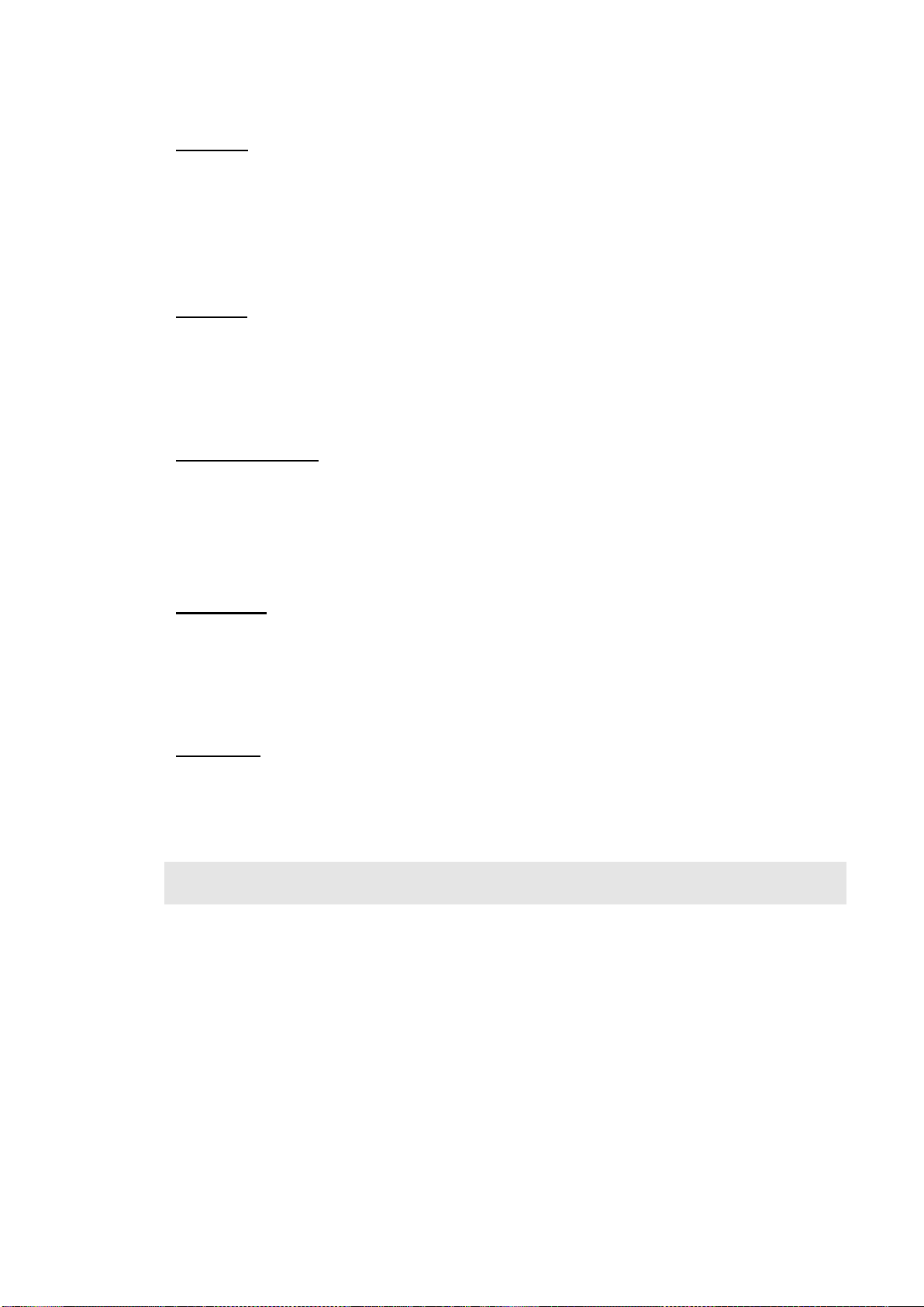
Surfaces
Press Surfaces if you want to measure surfaces. In this mode, measured data are rasterized
immediately after acquisition using the selected settings (see chapter 7.2.3). Besides, the value
for Close gaps will be used as well as the reflection filter defined in the materials editor (see
chapter 17.10).
Optionally you can select Surfaces in the Measurement toolbox by hitting Surfaces/Features.
Features
Press Features if you want to measure features like e.g. gaps or boundaries. In this mode,
measured data are not rasterized, but visualized as a point cloud. Close gaps will be
deactivated.
Optionally you can select Features in the Measurement toolbox by hitting Surfaces/Features.
Material selection
From the list of materials, select the one which resembles your object’s properties the most.
By default, the following materials are available: Standard, Shiny bright, Dark and Shiny dark.
You can add, modify or delete further materials using the Material Editor (see chapter 17.10).
Optionally you can select a material in the Measurement toolbox.
Close gaps
If gaps appear within a scan line, they can be filled automatically by means of interpolation.
Specify a value for the maximum gap size up to which a gap will be closed automatically.
This setting is useful when measuring surfaces like fabrics, felt, foam material or similar, and a
complete surface is required.
Line width
With this slider, you can reduce the width of the line to be scanned down to 40% of the
maximum width. By choosing a smaller line width, you can increase the line frequency.
Optionally you can modify the line width in the Measurement toolbox.
Note
Please note that the visible width of the laser line is not influenced by this setting.
Page 28
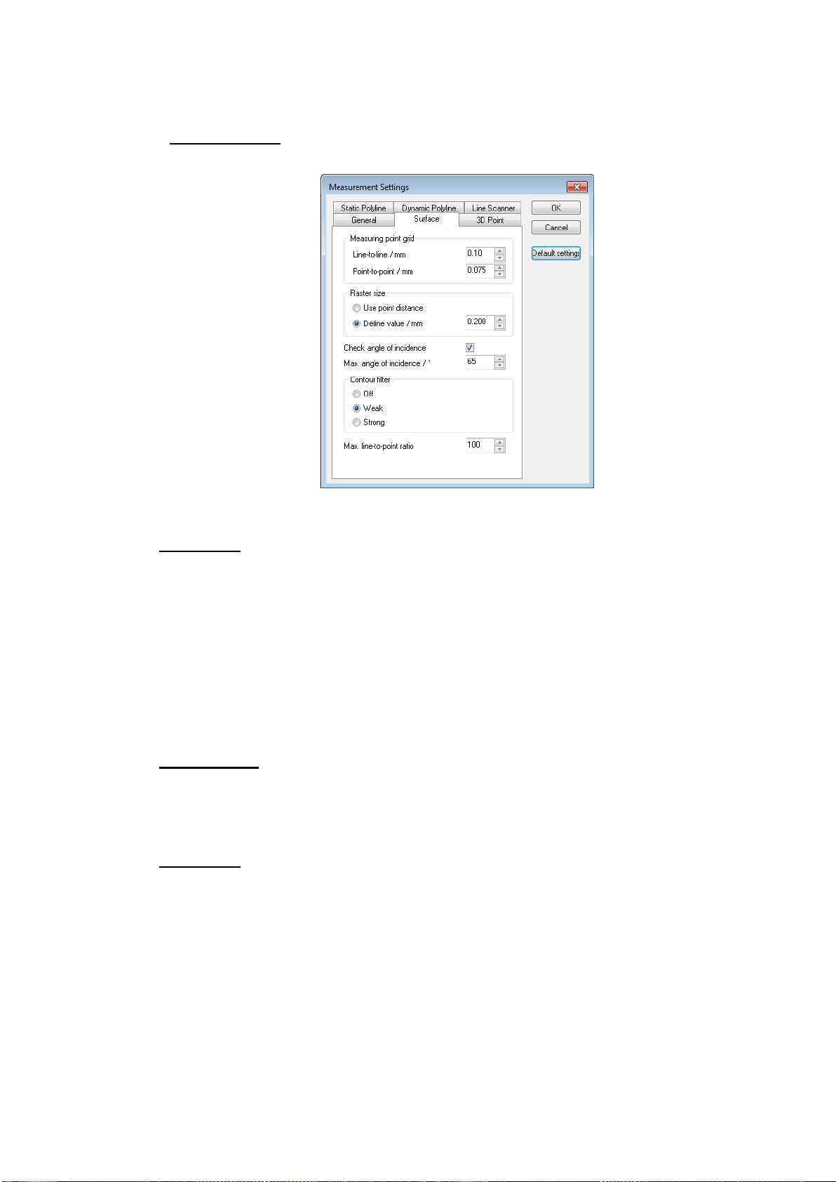
7.2.3 Surface Mode
Line to line
This value defines the minimum distance between two scan lines. The minimum distance
prevents the acquisition of too dense data if the scanner is moved very slowly or not at all. The
software checks if the scanner moved more than the entered Line to line value. If it did not,
the current scan line is rejected.
The absolute distance between the scanner positions is calculated, i.e. spatial movement in the
scan line direction also increases the distance. Only the distance to the previous scan line is
calculated. If the scanner is repeatedly moved over the same point, data is acquired with each
new movement.
Point to point
This value determines the average point distance on the scan line. It refers to the center of the
scanner’s measurement range and changes with increasing or decreasing distance to the
object. The value can only be changed in 0.075 mm steps.
Raster size
If the Use point distance radio button is selected, the raster width is set according to the point
to point distance.
If you want to use a different raster width, select Define value and specify the raster width.
Bear in mind that a raster width of less than 0.1 mm will dramatically increase the amount of
data generated.
Page 29
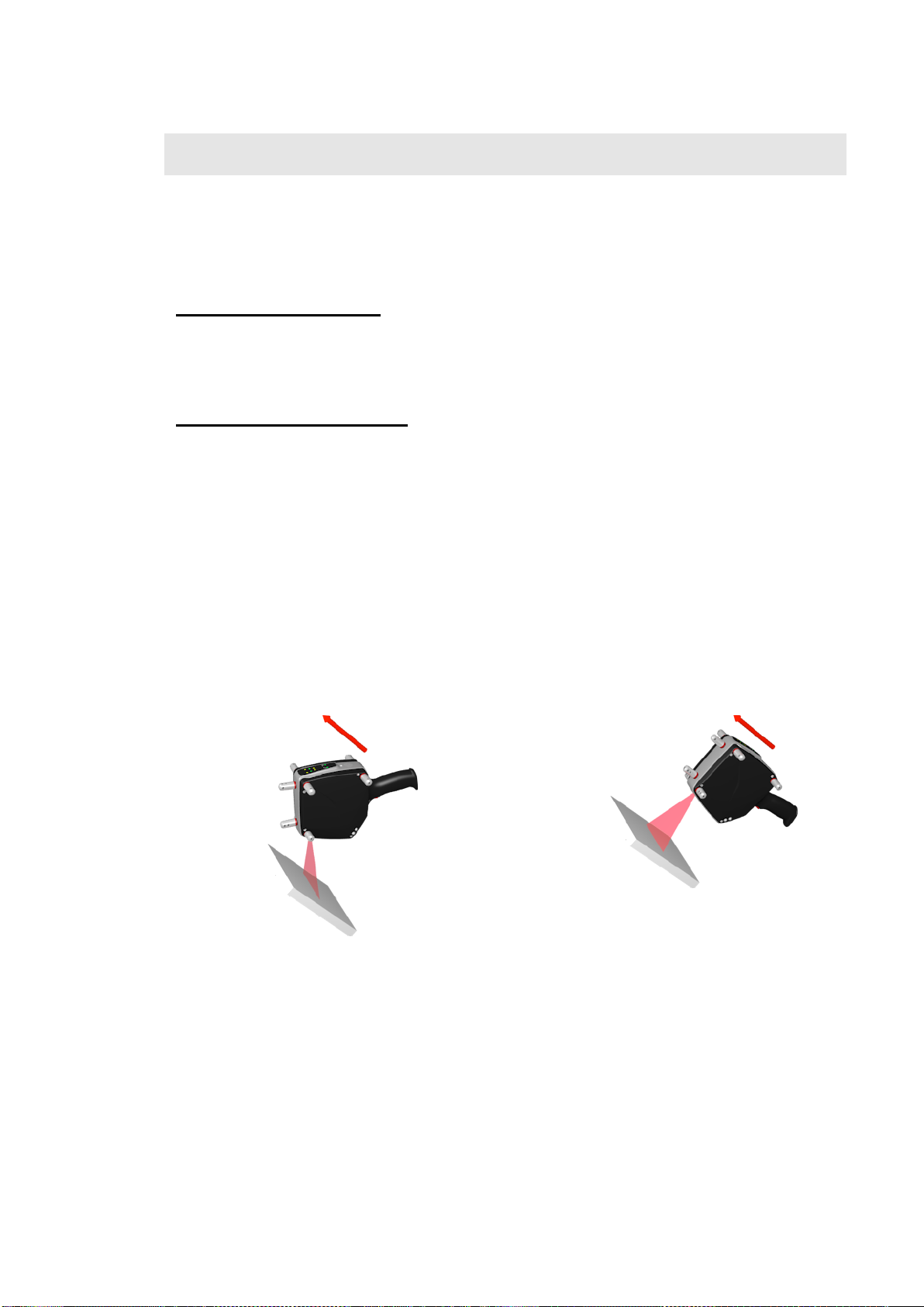
Note
Angle treatment when moving in the direction of motion
The angle between the laser plane and the
object exceeds the entered threshold: No
measurement data will be acquired.
Measuring correctly: The angle between the laser
plane and the object is almost perpendicular.
A rasterization process is started when
- the Measurement Settings for the Line Scanner is set to Surfaces (see chapter 7.2.2) or
- post-processing is started and the scene contains non-rasterized scanner data.
Check angle of incidence
If this checkbox is selected, a filter is applied to the data. The filter removes points measured
with an angle of incidence that exceeds the specified maximum value. How this filter works is
described in more detail below.
Maximum angle of incidence
Measured points for which the angle of incidence between the laser beam and the surface
exceeds the entered value are rejected. The smaller the value, the less data you will acquire,
but the higher the data quality will be.
The angle is initially checked within each scan line. If the Measurement Settings for the Line
Scanner is set to Surfaces (see chapter 7.2.2), the angle is additionally checked in the direction
of motion of the scanner.
The following illustrations demonstrate the principle of the filter. The arrow indicates the
direction of motion of the scanner.
Page 30
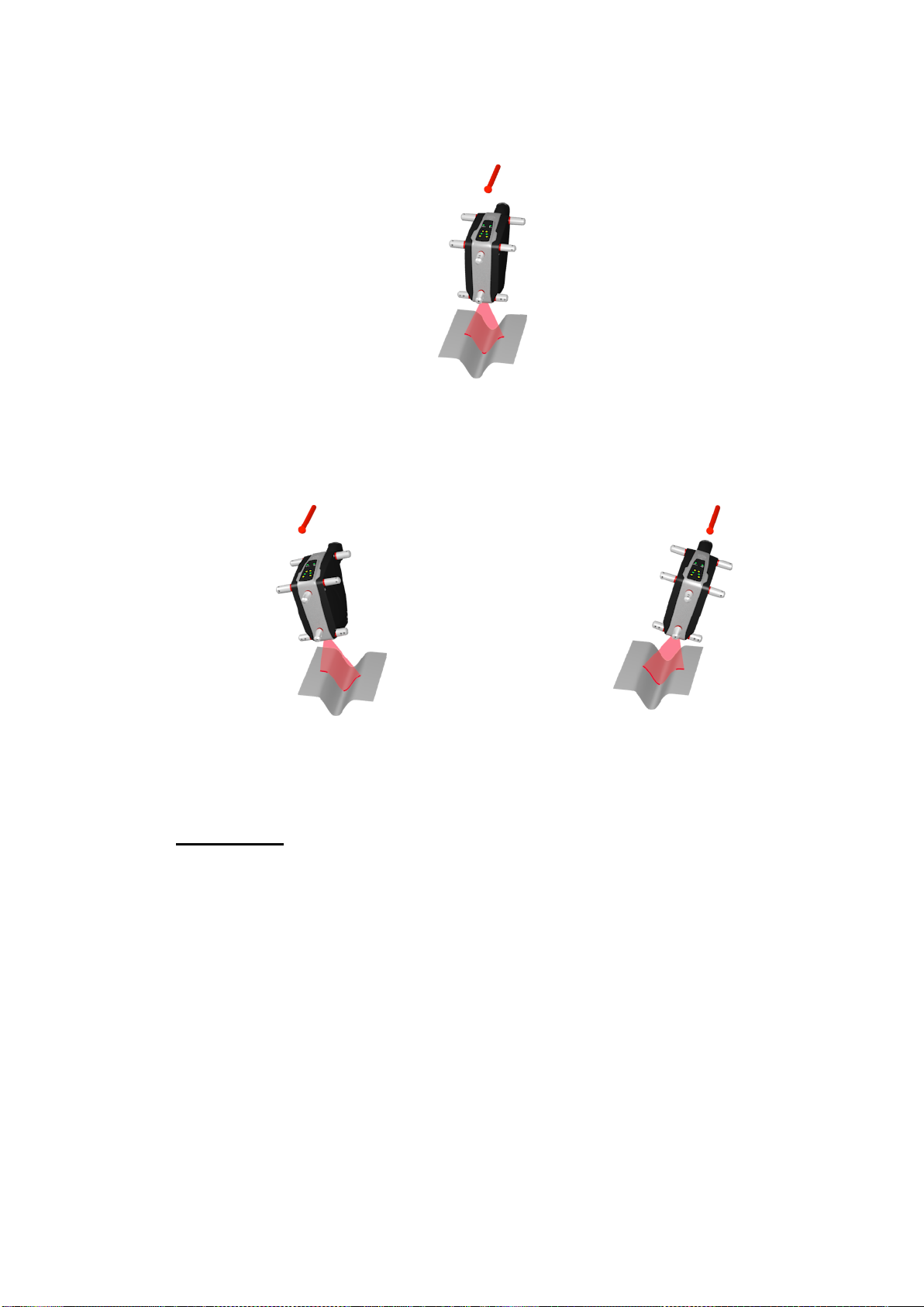
Angle treatment within a scan line
No measurement data is acquired if the angle between
the laser beam and the surface exceeds the entered
value.
To measure the surface completely, do two
scans. Tilt the scanner first in one direction...
...and then in the other direction.
Contour filter
This filter is only applied if the measurement settings for the Line Scanner is set to Surfaces
(see chapter 7.2.2). It can improve the data quality of the scan data when measuring
contoured objects using an inappropriate measurement strategy.
Page 31

Inappropriate measurement strategy: the
scanner is moved too fast and the scan line is
almost parallel to the object’s contour. The
contour filter will remove data.
If the scanner is moved too fast relative to the selected point-to-point distance and the scan
line is almost parallel to the object’s contour (see illustration), surface elements that do not lie
completely on the object surface might be created between neighboring scan lines. The
object’s contour will then look ‘blurred’.
The contour filter analyzes the points of neighboring scan lines and prevents the points from
being connected to a continuous surface if an inappropriate measurement strategy is used.
Therefore, gaps in the data may occur, providing a visual indication to the user that this area
should be measured again using a more suitable strategy.
The filter strength can be adjusted to achieve optimal data quality. If the filter is set to strong,
more data will be rejected. If the filter is set to weak, less data will be rejected; however, data
might then be retained that does not actually lie on the object’s surface. You can also disable
the filter if you want to keep the data in any case.
The measurement strategy described above should generally be avoided. Instead, you should
always try to measure perpendicularly to the object’s contours (see illustration below). Even if
the filter is set to strong, the algorithm will detect if an appropriate strategy has been used and
will retain all data.
Page 32

Appropriate measurement strategy: The scanner
is moved perpendicularly to the object’s contour. The contour filter will retain all data.
Max. line-to-point ratio
If the speed the scanner is moved over a measurement object is too fast relative to the
selected point-to-point distance, widely spaced scan lines will be created. When this data is
then rasterized, the point-to-point distance used is taken as the basis for rasterization. As a
result, the “gaps” between the scan lines may be filled (interpolated) with many points, which
excessively increase the data volume without improving the data quality.
Ideally, the scanner is moved fast enough so that the distances between points on a scan line
are approximately equal to the distances between neighboring scan lines.
If the ratio of “distance between scan lines” to “point distance within a scan line” exceeds the
specified value, these scan lines are not connected to create a continuous surface, but gaps are
left. This can help the user to optimize the measurement strategy and avoid unnecessarily
large data volumes.
7.2.4 3D Point Mode
Page 33

For this measurement mode, data is acquired and averaged internally. The averaged value is
output as a measurement point.
Measuring priority
This setting controls the method how a 3D point is measured. By default, the following options
are available: Precise, Standard and Fast.
Next ID
This field is only available in the settings for 3D points and defines the name for the next point
to be measured. If the ID does not end with a digit, a sequential number – beginning with “1” –
is automatically appended to the name.
7.2.5 Static Polyline Mode
The settings for these two modes are identical.
Page 34

For this measurement mode, data is acquired and averaged internally. The averaged value is
output as a measured point.
Measuring priority
This setting controls the method how a 3D point is measured. By default, the following options
are available: Precise, Standard and Fast.
Page 35

7.2.6 Dynamic Polyline Mode
Point frequency
The points will be acquired with the entered frequency.
Point-to-point distance
This value defines the minimum distance between two successive points. The minimum
distance prevents a too dense data recording if the T-Probe is not moved or moved very
slowly. The software checks if the T-Probe moved more than the Point-to-point distance value.
If not, the current point will be rejected.
7.3 Starting a Measurement
When you click the Start icon in the standard toolbar or choose Digitize Start, the scanner or
the T-Probe is activated in the selected measurement mode (Surface, 3D Point, Static Polyline).
The Start icon is disabled and the Stop icon is enabled.
7.3.1 Surface Mode
In Surface Mode, 3D points on the object’s surface can be measured with the T-SCAN scanner.
Page 36

The measurement itself is started as soon as you use the trigger button on the scanner handle.
T-Scan Collect automatically becomes the active application – depending on the settings (see
chapter 17.15) – if another application was active. You can make as many measurements as
required.
During measurement, 3D coordinates are calculated and the newly measured data is shown in
the selected color (typically red, see chapter 7.2.1).
If the measurement setting for the line scanner is set to Surfaces (see chapter 7.2.2), the data
is displayed in the default color immediately after it has been rasterized.
A new entry is created in the data explorer toolbox. If the measurement setting for the line
scanner is set to Features (see chapter 7.2.2), the entry is named “T-SCAN[sequential
number]”. The number is incremented with each scan.
If the measurement setting for the line scanner is set to Surfaces, a scan might be split up into
several parts. This happens if the scanner orientation changes significantly during a scan, thus
influencing the rasterization direction. In the data explorer, splitted scans are named “T-SCAN
[sequential number]_[sub number]”, where [sub number] always starts with 1.
7.3.2 3D Point Mode
In 3D Point Mode, single 3D points can be measured with the T-Probe. Depending on the
selected settings (see chapters 17.13 and 17.14), the T-Probe coordinates window and/or the
wireframe of the T-Probe will show up as soon as the measurement starts.
Page 37

To acquire a measurement point, press the trigger button on the T-Probe or press the <M>
key. As soon as the measurement was successfully completed, the measurement point is
displayed in green color. You can acquire as many measurement points as are required.
Note
Every measured point is stored in a separate data set and named according to the settings you
made (see chapter 7.3.2). If a data set of the same name already exists, another data set is
created using the next free number.
By pressing the <D> key, you can delete the points in the reverse order in which they were
acquired.
7.3.3 Static Polyline Mode
In Static Polyline Mode, single 3D points are measured with the T-Probe and automatically
connected to create line segments. This way, you can acquire polylines. Depending on the
selected settings (see chapters 17.13 and 17.14), the T-Probe coordinates window and/or the
wireframe of the T-Probe will show up as soon as the measurement starts.
To acquire a measurement point, press the trigger button on the T-Probe or press the <M>
key. As soon as the measurement was successfully completed, the measured point is visualized
Page 38

and connected to the previous point by a line. You can adjust the point size and line size (see
chapter 17.3) to optimize the visualization. A polyline may contain any number of points.
You can start a new polyline by pressing the <N> key. The last active polyline is closed and
displayed in blue.
Note
Polylines are saved in data sets named “Polyline[X]”, where [X] is a sequential number. If you
rename such a data set, it will not be treated as a polyline anymore.
Pressing <D> deletes points from the “Polyline[Y]” data set, where [Y] is the highest existing
number. If the last point of a polyline is deleted, the polyline itself will also be deleted. The next
delete action will open the data set with the now highest number and delete the last measured
point from that line.
7.3.4 Dynamic Polyline Mode
In Dynamic Polyline Mode 3D points can be measured continuously with the T-Probe. The
points will be connected automatically to form line segments. According to the settings (see
Page 39

chapters 17.13 and 17.14) the T-Probe coordinate window and/or the wire frame model of the
T-Probe will be displayed as soon as the measurement starts.
As long as the right mouse button or the button of the T-Probe is pressed, points will
continuously be acquired with the chosen settings (see chapter 7.2.6). By releasing the button,
the polyline will be completed. Pressing the button anew will create a new poly line.
Remarks
Lines will be stored in data sets named „Polyline[X]“ where [X] is a running number. If you
rename such a data set it will not be treated as a poly line anymore.
7.4 Stopping a Measurement
To stop a measurement, click the Stop icon in the standard toolbar or choose Digitize Stop.
The infrared LEDs are switched off and the scanner goes into sleep mode. The Start and Stop
icons change their states accordingly.
You can continue the measurement at any time. All you need to do is restart the
measurement. The measured data is added to the existing data.
Page 40

8 Interactive Tools
There are several interactive tools you can use for editing existing data sets. These tools are
provided in the ‘Interactive Tools’ toolbox and can also be accessed by selecting Edit
Interactive Tools or the drop down menu in the toolbar.
The toolbox contains the following tools:
Selection mode (“No Tool”)
Interactive clipping
Check accuracy
Cross sections
Create reference points
Fill holes / tools for editing triangle meshes
Alignment calibration
The Data Analysis tool is currently not used and therefore is not available
The tools and have a small arrow in the bottom right corner. The arrows indicate that a
submenu can be opened when clicking the icons and keeping the mouse button pressed.
The functions of these icons can be modified by selecting a menu item.
The tool currently in use is shown in the toolbar. A blue background indicates whether the tool
is active (“tool mode”) or inactive (“view mode”). By pressing <Space Bar> in the 3D viewer,
you can switch between these modes.
Page 41

8.1 Selection Mode
This icon activates the selection mode. When you click a data set in the 3D viewer, it is
displayed in the assigned selection color and shown in red in the data explorer (see chapter
5.4).
8.2 Interactive Clipping
This tool allows you to clip data of any type. If all data of an object or entire objects are
clipped, the corresponding entry is removed from the data explorer.
The toolbox offers the following options:
Choose whether the clipping action will apply to All faces, only Front faces or only Back
faces. This option is only effective for objects that have back and front faces.
If this option is enabled (symbolized by a “normal” eye), no data will be deleted that is
currently invisible, e.g. because it lies outside the 3D viewer or is hidden by other data. If the
option is disabled (“X-ray eye”), all the data within the selection will be deleted.
If this option is enabled, data within the selected area will be retained and all data outside
the selection will be deleted. The selected area will then be shown in green instead of red.
Move the mouse cursor over the area containing the data you want to edit. If view mode is
currently active, change to tool mode by pressing <Space Bar> in the 3D viewer.
Define the area to clip with the left mouse button. By left-clicking, you can define a straight
line. If you keep the left mouse button pressed, you can draw a continuous line. Close the area
by double clicking with the left mouse button or pressing the right mouse button. You can also
select multiple areas in this way.
Press or the <Enter> or <Del> key to clip the selected areas. Press to undo the last action
or actions you made.
8.3 Check Accuracy
With this tool, you can check the measurement accuracy of the T-SCAN system.
Page 42

1. Before running an accuracy check, it is advisable to review the nominal values in the
settings dialog :
1. If you are using a barbell, enter the sphere radii into the corresponding fields. Sphere 1
corresponds to the red, Sphere 2 to the blue sphere displayed in the toolbox. The
correct Distance between the two spheres also needs to be specified.
If you are using a single sphere, you are free to choose which field to use for the
nominal radius. Take care to select the correct sphere (red/blue) later in the
evaluation.
2. If Fit with free radius is disabled when you perform the accuracy check, the software
will try to fit a sphere with the given radius into the data. This may lead to an error
message if it is not possible to calculate a reasonable result, e.g. because the given
radius differs significantly from the actual data.
3. In the Remove outliers fields, you can specify how many of the worst fitting points will
be removed before sphere fit and plane fit. A setting of 1 Sigma will eliminate
approximately 32%, 2 Sigma approximately 5% and 3 Sigma approximately 3 ‰ of the
most off-size points.
4. For the sphere fit, Visible points only is disabled by default because, in most cases, you
will want to check the entire sphere, including the rear side.
For the plane fit, Visible points only is enabled by default because usually only the
Page 43

selected points are part of the plane, whereas surfaces or data sets located behind the
plane are to be left unconsidered.
2. Now use the lasso in the 3D viewer to select the first or the only sphere/plane you want
to check. Make sure that the correct sphere or plane is selected in the toolbox (red/blue).
Then start the evaluation by pressing <Enter> or clicking .
3. The following result dialog appears:
Example
for one sphere: for two spheres:
The results can be saved to a text file which can be imported into third party software (e.g.
Microsoft Excel).
Note
If you click the currently selected button ( , , , ) in the toolbox once more, the
result dialog is reopened and you can again view or save the available results. The values
remain stored even after the toolbox is closed, but will be deleted when you exit the
application.
4. Fitted objects (spheres or planes) are displayed in the 3D viewer. Their colors help to
identify their correspondences to the first fit (red) or the second fit (blue).
These objects are removed when the toolbox is deactivated or closed, or when switching
from sphere fit to plane fit (or vice versa).
5. If you want to check a second sphere or plane, select the correct icon in the toolbox (for
spheres normally , for planes normally ) and repeat step 2.
On completion of a calculation for spheres, a line connecting the two sphere centers in the
Page 44

3D viewer displays the determined distance.
Repeating a calculation will overwrite existing results.
6. The icon clears all results of the sphere and plane fits as well as the objects created in
the 3D viewer.
7. By default, the lasso is selected for creating the set of points for the fit. However, it is
also possible to create single points that will be used as the basis for the calculation. To do
so, switch to point mode .
You can now select points by left-clicking on the data. These points are displayed as small
spheres. As soon as at least four valid points have been selected, a preview object (sphere
or plane) is created and displayed in the 3D viewer. Every time you add a new point, the
preview is recalculated to make the changes visible. The final calculation is carried out
when you press <Enter> or click in the toolbox.
8.4 Cross Sections
When the cross sections toolbox is active, the following tools for creating cross sections are
available:
Page 45

The cross sections toolbox provides access to manipulation functionality for the cross
section plane . The cross section plane and, if activated, the auxiliary planes for multiple
sections, are visualized.
Selection of the cross section plane direction (along the coordinate axes)
Position of the cross section plane along the selected coordinate axis
Center the cross section plane in the data set
Open the dialog with the cross section settings; see chapter 17.1
Create multiple sections. If this mode is active, the step width field defines the distance
between multiple sections. Two auxiliary planes are displayed at the specified distance to the
main plane in the 3D viewer, providing a preview of the settings.
Calculate and display cross sections
Note
The following display settings will be used:
o Red, semitransparent: cross section plane
o White: bounding box
o Green: center lines of the cross section plane as well as the start and end points and
the intersection point of these lines.
8.5 Create Reference Points
With this tool, you can use sphere fits to create reference points from measurement data. The
following toolbox appears:
Page 46

1. Before creating a reference point, it is advisable to review the settings. Click on the
Settings button to open the dialog:
If Fit with free radius is disabled, the software will try to fit a sphere with the
given radius into the data. This may lead to an error message if it is not
possible to calculate a reasonable result, e.g. because the given radius differs
significantly from the actual data.
In the Remove outliers field, you can specify a factor which defines how many
percent of the worst fitting points will be removed in a sphere fit. The default
value is 0.003, meaning 3 ‰.
The Visible points only checkbox is deselected by default because, in most
cases, you will want calculate the fit for the entire sphere, including the rear
side. This checkbox can be selected if required.
2. Now use the lasso in the 3D viewer to select the data you want to use for the sphere
fit and press <Enter> or the toolbox icon .
3. The reference sphere is displayed as a blue sphere in the 3D viewer.
8.6 Fill Holes (Triangle Mesh)
This tool provides options for interactively or automatically filling holes in a triangle mesh. This
functionality is available if a single triangle mesh is loaded. The following toolbox appears:
Page 47

Holes can be selected in two different ways:
Move the mouse cursor over the triangle mesh area you want to edit. If view mode is
currently active, change to tool mode by pressing <Space Bar> in the 3D viewer. Holes
in the data set in the area near the mouse cursor are detected automatically and
shown with a yellow border. When you left-click a detected hole, the hole is filled and
a preview of the result is displayed.
Click the Previous Hole or Next Hole icon to select one hole after the other. The 3D
view can be automatically centered on the selected hole if icon is activated.
With the Density and Noise sliders, you can adjust the data generated for the filled
hole to optimally fit the characteristics of the surrounding measurement data. If multiple holes
are selected and filled, these settings are applied to each of them.
The Mode list box provides the following filling strategies:
flat fills a hole as plane as possible; works very fast
curved incorporates the orientations of the surrounding mesh into the calculations,
delivering excellent results e.g. when filling holes in spheres; calculation takes longer
To accept the generated areas, press the Apply icon or right-click in the 3D viewer. If you
are not satisfied with the result, click Undo to undo the last action or actions you made.
Holes can also be filled automatically. For this, enter the maximum Circumference in mm
and click . All holes up to this size are filled automatically using the specified settings.
The title bar of the toolbox shows information on how many holes have been detected in
the triangle mesh.
8.7 Create Bridges (Triangle Mesh)
This tool provides the possibility to interactively create bridges over gaps in a triangle mesh.
This functionality is available if a single triangle mesh is loaded. The following toolbox appears:
Page 48

Move the mouse over the triangle mesh area you want to edit. If view mode is currently active,
change to tool mode by pressing <Space Bar> in the 3D viewer.
To create bridges, move the mouse over the area to be edited until the area is highlighted in
yellow. Click on it with the left mouse button to define the start edge for the bridge. Then
select the end edge with the left mouse button. A preview bridge with the currently selected
parameters is displayed between the two selected edges.
In the Mode list box , you can choose between the following bridge modes:
Linear
This mode creates a linear data bridge as the shortest connection between the selected edges.
Tangential
This mode creates a data bridge between the selected edges, taking the surface orientation of
the adjacent triangles into account.
Corner
This mode creates two linear data bridges, one from each selected edge. The surface
orientation of the adjacent triangles is taken into account. The edge that is formed where the
two linear bridges meet can then be rounded with the Radius slider .
The selected mode can be changed even after you have selected the start and end edges. This
way you can visually adjust the generated bridge to the surrounding area.
To accept the generated bridge, press the Apply button or right-click in the 3D viewer. If
you are not satisfied with the result, click Undo to undo the last action or actions you made.
8.8 Smoothing (Triangle Mesh)
With this tool, you can interactively smooth areas in a triangle mesh. This functionality is
available if a single triangle mesh is loaded. The following toolbox appears:
Page 49

Move the mouse over the triangle mesh area you want to edit. If view mode is currently active,
change to tool mode by pressing <Space Bar> in the 3D viewer.
A circle is displayed around the mouse cursor showing the radius of effect of the tool (“brush
size”). It can be resized with the mouse wheel or by drag and drop with the middle mouse
button.
To smooth an area, left-click on the beginning of the area and keep the mouse button pressed.
Now drag the cursor over the desired area on the object. The data in this area is smoothed
while you move the cursor. Releasing the mouse button stops the smoothing process.
The smoothing strength can be adjusted with the Strength slider .
If you are not satisfied with the result, click Undo to undo the last action or actions you
made.
Note
Take care to only smooth surfaces that face the user in the 3D viewer. Smoothing transitions
from front side to back side (e.g. on spheres), or on faces which can only be seen under a very
small angle, can lead to artifacts.
8.9 Decimate Mesh (Triangle Mesh)
This tool is used to interactively decimate a triangle mesh. This functionality is available if a
single triangle mesh is loaded. The following toolbox appears:
Move the mouse over the triangle mesh area you want to decimate. If view mode is currently
active, change to tool mode by pressing <Space Bar> in the 3D viewer.
A circle is displayed around the mouse cursor, showing the radius of effect of the tool (“brush
size”). It can be resized with the mouse wheel or by drag and drop with the middle mouse
button.
To decimate an area, left-click on the beginning of the area and keep the mouse button
pressed. Now drag the cursor over the object to mark the area you want to decimate. When
you release the left mouse button, the marked area is automatically decimated.
The Max. error parameter defines the maximum permissible deviation in millimeters; the
Max. edge length parameter defines the size of the resulting triangles in millimeters.
If you are not satisfied with the result, click Undo to undo the last action or actions you
made.
Page 50

8.10 Sharpen Edges (Triangle Mesh)
This tool provides the possibility to sharpen edges of triangle meshes interactively. This
functionality is available if a single triangle mesh is loaded. The following toolbox appears:
Move the mouse over the triangle mesh area you want to edit. If view mode is currently active,
change to tool mode by pressing <Space Bar> in the 3D viewer.
A circle is displayed around the mouse cursor, showing the radius of effect of the tool (“brush
size”). It can be resized with the mouse wheel or by drag and drop with the middle mouse
button.
To sharpen edges, left-click on the beginning of the area and keep the mouse button pressed.
Now drag the cursor over the object to mark the area you want to modify. When you release
the left mouse button, the edges in the marked area are automatically sharpened.
The Min. Angle parameter defines the minimum angle an edge must have in order to be
sharpened. A theoretical value of 0 means that all data is modified, a value of 180 means that
no data is modified.
If you are not satisfied with the result, click Undo to undo the last action or actions you
made.
8.11 Alignment Calibration
How to use this toolbox is described in detail in chapter 0 Calibration.
Page 51

9 Calibration
Environmental influences (such as temperature changes or transport of the system) may lead
to a gradual decrease in data quality.
To increase data quality, T-Scan Collect offers the alignment calibration feature which the user
can – and should – perform on site if:
an upcoming measurement requires highest accuracy
local accuracy has decreased. This can manifest itself, for example, in poor statistics
when calculating a sphere fit
gaps occur in the data
wavy data is measured on actually planar surfaces
9.1 Calibrate measurement range
9.1.1 Preparation
In order to perform the measurement range calibration, you need a planar surface with diffuse
reflection.
Not suited are surfaces containing scratches, bumps, dents or similar faults. In general, a table
board should suffice the requirements. However, it is recommended to use a specified plane
which is optionally available.
9.1.2 Procedure
Open the Measurement range toolbox. The measuring mode Alignment will automatically be
activated. When opening the toolbox the status – symbolized by the traffic light – will be set to
red by default, indicating that no action has been performed yet.
To perform the calibration, two measurements have to be made. Take care to account for the
following:
The distance between scanner and plane has to be as constant as possible
The laser should hit the plane perpendicularly
The markers of the used scanner face should point as directly as possible towards the
camera
The orientation of the scanner must not change during measurement
Each measurement must contain at least 5000 points
For both measurements, the same scanner face must be used
Both measurements must be made on the same area of the plane
Page 52

First measurement: keep scanner distance
constant (Close End*)
Second measurement: keep scanner distance
constant (Far End*)
*: For the definitions of these terms, see graphics in chapter 17.12.
Avoid measurements where the laser does not
hit the surface perpendicularly
Avoid measurements where the laser does not
hit the surface perpendicularly
Avoid tilting the scanner, so the markers do not
point directly towards the camera
Avoid changing the distance of the
scanner to the surface
The above sketches are drawn from the camera’s perspective.
Page 53

Now measure the plane one time using the Close End of the scanner and another time using
the Far End of the scanner (“Calibration measurement”).
In the 3D viewer, select the two data sets using the lasso. Take care not to select points which
do not lie on the plane. If other data (e. g. from previous measurements) is located at the same
area, hide or delete it in the Data Explorer toolbox prior to using the lasso.
Press Verify. If the data does not suffice the requirements an adequate message box will open.
In this case, repeat the measurement. Otherwise the status indicator will show you the status
of the measurement range calibration:
Green state: The scanner is calibrated optimally. No further steps are necessary and
you may close the toolbox.
Yellow state: The scanner calibration has been optimized using the measured data. To
make sure that the optimization improved the calibration it is necessary to measure
the plane again (in the same way as described above) one time using the Close End of
the scanner and another time
Red state: The scanner calibration has not been started yet or the Undo button was
pressed.
Page 54

If the Verification measurement confirms an improvement, the status indicator will switch
to green. In this case, save the new calibration by pressing Apply.
Otherwise the status indicator will remain yellow. You now have the possibility of either
repeating the verification measurement or undoing the calibration measurement by
pressing Undo.
If you are not able to reach the green status, you can close the toolbox. All changes will be
undone after a confirmation message box is displayed.
When closing the toolbox, the measuring mode which has been active before will be restored.
9.2 Alignment Calibration
9.2.1 Requirements for an Alignment Sphere
To do an alignment calibration, a high-precision calibration sphere is needed. It is
recommended to use a sphere made of ceramic, steel, aluminum or other suitable materials
with a diffusely reflecting surface (non-volumetric scattering), specified by Leica Geosystems.
These spheres are between 40 mm and 105 mm in diameter. The form error and the radius of
such a sphere are known with an uncertainty of less than 20 µm. A calibration certificate is
shipped with these spheres (e.g. Leica Reference Sphere – Article number: 576190).
9.2.2 Measurement Strategy
The Alignment has to be done for each face separately. For the left, top and right face there
are 5 main positions, for the back face there are 4 main positions:
Page 55

Left face
Top face
Back face
Right face
Page 56

For each main position 11 scans need to be acquired:
Center position
3 scans: Middle, left, right
Rotated to the left
3 scans: Middle, left, right
Rotated to the right
3 scans: Middle, left, right
Centered, diagonal
1 scan
Centered, diagonal
1 scan
Page 57

9.2.3 Step-by-Step Guide
1. Open the Alignment toolbox.
The Alignment measurement mode is activated automatically.
2. Press Start.
3. Measure the alignment sphere as described in chapter 9.2.3. Data measured in
Alignment mode is displayed in green by default to distinguish it from other data.
4. Press Stop.
5. If data was acquired that does not belong to the sphere (e.g. mounting, table, ...) you
can manually remove this data (see “Interactive Clipping” toolbox) or have this data
removed automatically. For this, activate Autom. clipping in the toolbox.
Note
Automatic clipping might lead to unexpected results if the initial data is inappropriate.
For example, if the majority of the data consists of the mounting or table, etc. (but not
the sphere) or if the scanner is way out of calibration, data fragments might remain
which normally should be removed. In this case, the data needs to be clipped manually.
6. You need to measure at least 400 000 points in order to continue. It is recommended
to measure between 400 000 und 1 000 000 points.
7. In the toolbox, enter the radius of the sphere given in the calibration certificate and
the maximum number of iterations . The recommended value is 250; however, the
algorithm often takes fewer iterations.
8. Press Start calculation .
9. The calculation may take several minutes, depending on the performance of the
computer and the initial calibration state.
10. After this calculation, a sphere fit is executed automatically.
11. A dialog appears, showing the results of the calibration and of the sphere fit:
Page 58

Check the color of the traffic light symbol and follow the displayed advice.
If a red traffic light appears, please check whether a correct radius value was entered.
A yellow light indicates a significant improvement in comparison to the previous state.
It is recommended to repeat the calibration in order to verify the result. A green state
means that some minor changes have been identified in the calibration, but no
significant improvement, i.e. the scanner is either optimally calibrated or this
calibration method cannot achieve further improvement.
The quality of the calibration result can only be assessed from the Before and After
information. To view this information, click Details…
In the details view, you can save the calibration results to a file.
If you cannot achieve the green state, even after repeatedly measuring the sphere, this
may be for the following reasons:
Bad measurement strategy; measure as described in chapter 9.2.3.
Setup changed, vibrations, instable setup; stabilize the setup
Scanner out of calibration; contact service personnel
Page 59

12. When you click Apply, the result of the calculation is applied to the actual calibration.
13. To verify the alignment, repeat the alignment measurement from step 3 as described
above.
14. When you close the alignment toolbox, the measurement mode that was active before
is restored.
Page 60

10 Working with Files
All file-related commands are provided in the File menu. The available commands are
described in detail below.
10.1 Create New Project
To create a new project, click New in the standard toolbar or choose File New. If new or
changed data is still in memory, a dialog appears asking if you want to save the changes. If you
press No, all data will be cleared from memory; if you choose Yes they will be saved to a file.
If an online transformation was created (see chapters 11.1 and 15.9), a dialog appears asking if
you want to keep or discard the current transformation.
10.2 Open Existing Project
To open a saved project (.TSC file), click Open in the standard toolbar or choose File
Open....
A file selection dialog appears where you can select the file path and the name of the project.
10.3 Save Project
To save the current project under the given project name, click Save in the standard toolbar or
choose File Save....
If you have not yet assigned a project name, the Save as... function described below is invoked
automatically.
10.4 Save Project Under New Name
To save the current project as a .TSC file under a new name, click Save as in the standard
toolbar or choose File Save as....
A file selection dialog appears where you can enter the file path and the name of the project.
You do not have to add the file extension .TSC explicitly; it is automatically added by the
software.
Example: Generate a project ...\Module\Module.tsc by changing to (or creating) the file path
'..\Module' and entering 'Module' in the File Name text field.
10.5 Import Data
You can import data in different formats into your current project by using the File menu or
the data explorer.
Page 61

10.5.1 Using the File Menu
If you want to add data to a specific group, you first have to select the group or a data set from
that group. Then click Import in the standard toolbar or choose File Import....
In the file selection dialog, select the file path and the file(s) to be imported, then click the
Open button. The selected files are imported and inserted into the selected group.
10.5.2 Using the Data Explorer
In the data explorer, right-click on a group or a data set within a group. Choose Import... from
the menu that opens. Then continue as described in chapter 10.5.1.
Note
To facilitate finding the file(s) to be imported, select the appropriate file type in Files of type
first. The file selection dialog will then only show files of this type.
You can import several files (of the same file type) in a single step by multiple selection in the
selection dialog.
10.5.3 Using Drag and Drop
Files known to the software can also be imported by drag and drop to the 3D viewer or the
data explorer toolbox. When importing to the data explorer, the data will be placed in the
group over which the mouse button was released.
10.6 Export Data
You can export the loaded data sets in different formats. This is especially useful if you want to
process the data in a different application.
You can export data using the File menu or the data explorer.
10.6.1 Using the File Menu
This function is available if measurement data is provided in memory. To export 3D data, press
Export in the standard toolbar or choose File Export....
In the file selection dialog, select the file path on which the created file is to be saved. Enter a
name and select the file format to be generated.
Set the other options as required and then click the Save button.
Note
Please keep in mind that, with some file types, not all the data can be exported in the selected
format. The following table shows the data supported by the individual file types.
Page 62

TSC
AC
ASC
TXT
IGS106
IGS110
IGS116
SBP
SBT
STL
VDA
LST
CGK
Hierarchy (Data Explorer)
Unstructured Pointset
LineScanSet
RangeImage
PolyLine
PolyLineSet
Point
Triangle Mesh
Alignment Data
: Export fully supported
: Export not supported
: Data will be exported as Unstructured Pointset
: Data will be exported as PolyLineSet
: Data will be exported as PolyLine
10.6.2 Using the Data Explorer
In the data explorer, select the data sets you want to export. Right-click on one of the selected
data sets and select Export… in the menu. Then continue as described in Chapter 10.6.1.
Page 63

11 Processing of Data Sets
All processing functions are provided in the Edit menu.
11.1 Transform Data
To transform all loaded data sets, choose Edit Transform data. The following submenu
appears:
11.1.1 Transform
Choose Edit
Transform data Transform. The following dialog appears:
The different entries have the following meanings:
Mode of operation
With this parameter, you can choose how to determine the transformation matrix that will be
applied to all data sets. The following modes are available:
Online-Transformation
In this mode, the currently used online transformation is displayed. By clicking the Reset
button, you can undo the displayed online transformation.
Page 64

Use transformation file
In this mode, you need to specify a transformation file. The rotation angles and the
translation values are stored in this file.
Use given values
In this mode, the rotation angles and the translation values to be applied need to be
entered in the input fields.
Use viewing direction
In this mode, you can rotate the data sets in the 3D viewer before calling the function.
The data sets can be rotated in such a way that the viewing direction represents the
future positive Z axis. The X and Y axes will then be parallel to the monitor edges. During
execution of the function, a corresponding transformation matrix is calculated and
applied.
Transformation file
With this parameter, you determine the transformation file to be used. You can also determine
the file interactively in a file selection dialog by using the ... button next to the file name. The
field is only active if the mode of operation is set to Use transformation file.
Rotation, Translation
In these fields, you can define the rotation angles and the translation values from which the
transformation matrix is generated. The fields are only active if the Mode of operation is set
to Use given values.
Note
The symbol in the status bar indicates that an online transformation is active.
Please note that repeated execution of this function may lead to unexpected results!
11.1.2 Transform to Nominal Points
This wizard helps you to transform your data to the object’s coordinate system if nominal
points (e. g. from a CAD file) are available for the data set.
11.1.2.1 Edit the nominal points
Choose Edit
Transform data Transform to nominal points. A wizard will appear to guide
you through the process. You can cancel the wizard at any time by clicking the Cancel
button.
Page 65

With the wizard, you can load, save and manually edit nominal point lists.
The following functions are available:
Input box: ID
This input box defines the ID that will be assigned to the next point to be created.
Input box: X | Y | Z
These input boxes define the X, Y and Z components of a nominal point. As soon as one of the
input boxes loses the focus (by pressing <Tab> or clicking in a different area), a nominal point
with the respective ID is either created and added to the list, or an already existing point is
modified.
Nominal scaling (1:N)
The nominal scaling helps you if the measurement object and the nominal points are scaled
differently (e. g. if the scale of the object is 1:4 and that of the nominal points is 1:1). The
nominal data is automatically scaled to the correct size. For example, if the scale of your model
is 1:4, enter a value of 4; if the scale is 2:1, enter 0.5.
Columns: ID | X | Y | Z
This table shows the nominal points. By using the checkbox in the ID column, you can specify
whether a point will be used for calculating the transformation. If you deselect the checkbox,
all three coordinates of the point are grayed out and the point will not be used in the
calculation.
Page 66

With the right mouse button, you can exclude individual coordinate components of a point
from the calculation. When you right-click the component of a point, its state changes from
active to passive, and vice versa. Use this possibility if not all coordinates of a nominal point
are known or are to be used.
Excluding the X coordinate of a nominal point
When you click an ID in the first column, the point is selected and the ID is displayed with a
blue background. You can use the input boxes to modify the point you last selected.
Delete
Use this button to delete the currently selected points from the list.
Note
You can also delete selected points by pressing <Del>.
Delete All
Use this button to delete all points in the list.
Load
Opens a file selection dialog to load a point list file.
Save
Opens a file selection dialog to save the point list file.
The Next button is available as soon as enough points or components have been selected.
Note
If you press Next without having excluded any coordinate components of a nominal point, you
will not be able to exclude them later. If this has become necessary, however, please close the
wizard and re-open it (save your nominal points beforehand, if required).
11.1.2.2 Measure the actual points
On this page, you create the corresponding measurement points for the points you selected on
the Edit the nominal points page.
The next steps in the wizard depend on whether you have excluded coordinate components of
the nominal point from the calculation.
Page 67

If no coordinate components were excluded, the correspondences between the measured
points and the nominal points are determined automatically.
If coordinate components were excluded, you need to define the correspondences manually
through the ID, i.e. by measuring the points in the correct order.
The following functions are available:
Column: ID
If coordinate components were excluded, the IDs of previously measured points are displayed.
When measuring points, please make sure the correct ID is selected.
If no coordinate components were excluded, the ID column is initially empty. The IDs will be
computed automatically in the next step when the transformation is calculated.
Columns: X | Y | Z
Displays the coordinates of measured points. If coordinate components were excluded, points
that have not yet been measured are marked with a “---” symbol.
From Scene
If no coordinate components were excluded, all points from the data explorer are entered in
the table. If coordinate components were excluded, only those points are entered that match
the name of a loaded point.
Page 68

Measure
When you click this button, the point you last selected in the table is measured with the
T-Probe. If the measurement succeeded, the next point in the list is automatically selected.
Note
You can also start a measurement by clicking the right mouse button or pressing <M>.
Delete
Use this button to delete the coordinates of the currently selected points from the list.
Note
You can also delete the coordinates of selected points by pressing <Del>.
Delete all
Use this button to delete the coordinates of all points in the list.
Load
Opens a file selection dialog to load a point list file. If coordinate components were excluded,
only those points are imported that match the given IDs. The other points are ignored.
Save
Opens a file selection dialog to save the point list file.
The Next button is available as soon as enough measurement points have been acquired.
11.1.2.3 Transformation results
This page shows the calculated best fit transformation as well as statistics for the best fit.
Page 69

Columns: ID | X | Y | Z
The first column of the table shows the ID, the other columns show the X, Y and Z coordinates.
Three rows are displayed for each ID:
Nom: This row shows the nominal values as entered on the Edit the nominal points page of
the wizard (if applicable, scaled by the nominal scaling factor).
Act: This row shows the measured points after they have been transformed to the nominal
points.
Dev: This row is displayed in red on a gray background and shows the deviation between
actual point and nominal point.
Coordinates that have been grayed out on the Edit the nominal points page will be excluded
from the calculation and are therefore displayed in gray.
Rotation / Translation
These fields display the calculated rotation (in degrees) and translation (in millimeters).
Statistics
The statistics provide information on the best fit. The first line shows the maximum 3D
deviation and the ID for which the deviation was determined. The second line indicates the
minimum 3D deviation and the corresponding ID, followed by the mean 3D deviation and the
3D standard deviation.
Page 70

By pressing the Back button, you can access the previous pages of the wizard and make
modifications. If no coordinate components were excluded, the corresponding IDs that have
been calculated automatically are now displayed as well.
For example, you can exclude the ID that shows the maximum 3D deviation from the
calculation by returning to the Edit the nominal points page and deselecting that specific point.
Alternatively, you can also measure the point again.
When you click the Finish button, the measured data is transformed to its origin with the
inverse of the current online transformation. The newly calculated transformation is then
applied. In this way, you can repeatedly execute the Transform to nominal points wizard.
Log file
Use this button to save the results to a log file.
Note
When you apply the calculated transformation, you can visualize the nominal points in the 3D
viewer. Click the Nominal points icon in the 3D viewer toolbox.
The symbol in the status bar indicates that an online transformation is active.
11.1.3 3 Planes Alignment
To align all loaded data sets by using reference planes, select Edit Transform data 3
planes alignment. The following dialog appears:
Page 71

Use the provided tools to select all reference planes one after the other and assign the
respective point data to paraxial nominal planes.
The following drawing tools are available:
Shape of selection: rectangle, circle, ellipse
Shape of selection: polygon
Confirm the shape created with tool
Discard an unconfirmed shape created with tool
Drawing mode
Viewing mode
Assign the object data of the masked area to a nominal plane perpendicular to the X, Y or Z
axis
Page 72

As soon as you click one of the tools , you need to define the position of the plane in the
following dialog:
When you click OK, a plane fit is calculated based on the selected points, and plausibility
checks are performed for planarity of data, angles to already created planes, etc. After
successful completion of the best fit, the plane object is added to the list of reference objects.
The masked points of the object are displayed in green.
As soon as at least one object has been assigned to each main plane, the Transform data
button is available. When you click the button, the data is transformed and the alignment is
completed.
Note
When using one of the tools , you can add areas in the following way:
1. Move the cursor to the top left corner of the area to be drawn.
2. Press and hold the left mouse button.
3. Move the cursor to the bottom right until the object has the required size.
4. When you release the left mouse button, the object is surrounded by a border that allows
manipulating the object: When the cursor is inside the object, you can move the whole
object; when the cursor is above one of the small squares, you can move the corresponding
border(s). To do so, press and hold the left mouse button, move the element to the required
position and release the mouse button.
5. To accept the object, use tool or double-click outside the drawn object with the left
mouse button. To delete the object, use tool .
When using tool , proceed as follows:
1. Move the cursor to the starting point of the polygonal chain and click the left mouse
button.
2. When you move the cursor, you can see a line between the last point and the cursor. Each
time you click the left mouse button, you add a new point to the polygonal chain. Repeat
this step until all points have been added.
3. To end the polygonal chain, double-click the left mouse button. Please keep in mind that
the point that is double-clicked is also added to the polygonal chain.
Page 73

Basically you can assign any number of reference planes to a main axis plane – also at different
axis positions. You need to make sure, however, that you only select the data of a single plane
and a single position in each step. Also be careful that no data from other areas is accidentally
selected as well. This mainly happens if data on the back of the object is hidden by front areas.
The symbol in the status bar indicates that an online transformation is active.
11.1.4 3-2-1 Alignment
To do a 3-2-1 alignment for all loaded 3D data sets, choose Edit Transform data 3-2-1
Alignment. The following dialog appears:
In the left part of the window, the loaded 3D data is displayed. Below the 3D viewer, the status
bar indicates how to use the individual tools. On the right, you will find the data explorer
with the project. Above it, there are several tabs with the different tools for orientation of the
3D data. During 3-2-1 alignment, alignment elements (planes, vectors, points) are created and
saved in a separate group of the 3D scene. These elements will be deleted when you leave this
dialog.
Page 74

The tools are grouped as follows:
Functions and tools for the extraction of alignment elements (planes, vectors,
points) from 3D data.
Functions and tools for the calculation of alignment elements from existing
alignment elements.
Functions and tools for the manipulation of alignment elements.
Functions and tools for 3D viewer control.
Tools for the generation of a best fit plane for the selected area in the 3D data.
Activate this tool and use the mouse to draw one or more polygons in the 3D data.
The polygons define the area for the calculation of the best fit plane. A polygon
point is defined by left-click. Double-clicking the left mouse button ends a polygon.
To start the calculation of the best fit plane, press the <F2> key.
Tool for the generation of a best fit plane for selected points of the 3D data.
Activate this tool and use the mouse to define points in the 3D data. These points
will be used for the calculation of the best fit plane. A point is defined by left-click.
To start the calculation of the best fit plane, press the <F2> key.
Function for the generation of points from the 3D data. Activate this tool and use
the mouse to define points in the 3D data. A point is defined by left-click.
Tool for the calculation of the main axes of inertia for the selected area in the 3D
data. Activate this tool and use the mouse to draw one or more polygons in the 3D
data. The polygons define the area for the calculation of the main axes of inertia. A
polygon point is defined by left-click. Double-clicking the left mouse button ends a
polygon. To start the calculation of the main axes of inertia, press the <F2> key.
Important: This function is only available for triangle meshes.
Tool for the generation of a best fit cylinder for the selected area in the 3D data.
Activate this tool and use the mouse to draw one or more polygons in the 3D data.
The polygons define the area for the calculation of the best fit cylinder. A polygon
point is defined by left-click. Double-clicking the left mouse button ends a polygon.
To start the calculation of the best fit cylinder, press the <F2> key. Since not the
cylinder but its axis will be used for the alignment, the cylinder axis is displayed as a
vector after the fit has been performed.
Tool for the generation of a best fit cylinder for selected points of the 3D data.
Activate this tool and use the mouse to define points in the 3D data. These points
will be used for the calculation of the best fit cylinder. A point is defined by left-
Functions for the Generation of Alignment Elements from 3D Data
Page 75

click. To start the calculation of the best fit cylinder, press the <F2> key. Since not
the cylinder but its axis will be used for the alignment, the cylinder axis is displayed
as a vector after the fit has been performed.
Tool for the calculation of the boundary planes of the 3D data for a selected area of
the 3D data. The generated boundary planes are parallel to the XY, XZ and YZplanes, respectively, of the current coordinate system.
Functions for the Generation of Alignment Elements from Existing Elements
Function for the generation of a point
For 3 Planes, the generated point is the point of intersection of the 3 planes
For Vector and Plane, the generated point is the point of intersection of vector
and plane
For Point and Plane, the generated point is the projection of the selected point
on the selected plane
For Circle, the generated point is the center of the circle
Function for the generation of a vector
For Plane, the generated vector is the normal vector of the plane
For Polyline, the generated vector represents the line of best fit through the
points of the polyline
For Two Points, a vector is generated with the selected starting and end points
For Two Planes, the generated vector represents the line of intersection of
these two planes
For a Point and a Plane, the generated vector has the selected starting point,
and it is normal to the plane
For a Vector and a Plane, the generated vector is the projection of the selected
vector on the selected plane
Function for the generation of a plane
For Three Points, a plane is generated which is defined by the selected points
For Circle, the generated plane is a circle plane
For Vector, the generated plane is normal to the vector and passes through the
starting point of the vector
Depending on the selection status of existing elements in the 3D data explorer, different
functions are available for the generation of additional elements.
Page 76

Functions for the Manipulation of Alignment Elements
This function is used to reverse the direction of all selected vectors in the scene
explorer
This function is used to reverse the direction of all selected planes in the scene
explorer
This function is used to translate all selected planes in the scene explorer in normal
direction. The translation distance is the value set in the input field
Functions for 3D Viewer Control
The buttons and the functions they represent are identical to those in the main window.
Please refer to that chapter for detailed information.
Execution of the Alignment
After the elements required for the alignment have been created with the above tools, the
elements that are to be used for the alignment of the 3D data are specified in the selection
fields. You can also drag and drop elements to be used for alignment directly into the selection
fields from the scene explorer.
Start the alignment by clicking the Align button. The dialog for the alignment settings is
displayed:
In this dialog, you can define the plane that will be used as the best fit plane in the new
coordinate system (please note that the direction of the plane’s normal vector will be taken
into account in the alignment). In addition, you can specify the axis that will be used as the
best fit vector in the new coordinate system, and the coordinates of the selected point in the
new coordinate system. Click OK to execute the alignment. You can undo the last performed
alignment with the Undo button.
Note
The symbol in the status bar indicates that an online transformation is active.
Page 77

11.1.5 Scale
To scale all loaded data sets, choose Edit Transform data Scale. The following dialog
appears:
Enter the factor and start the calculation by pressing OK.
11.1.6 Mirror
To mirror all loaded data sets, choose Edit Transform data Mirror. The following dialog
appears:
Select the mirror direction and start the calculation by pressing OK.
11.2 Optimize Data
11.2.1 Smoothing
To optimize all loaded, rasterized data sets, choose Edit Optimize data
following dialog appears:
Remove isolated points
If you choose this option, isolated points will be removed from the data.
Smoothing. The
Smooth data
If you choose this option, the data will be filtered with the following filter parameters:
Page 78

Strength of filter
Determines the strength of the filter. Valid values are in the range of 0 (no filtering) to 1
(strong filtering).
Weighting factor of edges
Determines the weighting of object edges. Valid values are in the range of 0 (object edges will
not be specially treated and will be filtered) to 1 (object edges will not be filtered).
11.2.2 Decimating
To systematically decimate visible data sets, choose Edit Optimize data
following dialog appears:
When you click OK, only every x
th
value in each column and every yth value in each row of each
data set will be kept.
Decimating. The
This function is effective for the following data types: rasterized and non-rasterized data,
unstructured point clouds and polylines.
11.3 Matching
11.3.1 Global Matching
If you used the Move Station Wizard (see chapter 15.9), all data will be in the same coordinate
system. However, depending on the accuracy and position of the reference points, the result
may still show deviations in the overlapping area. These deviations can be minimized by
matching. To start global matching, choose Edit Matching
following dialog appears:
Global Matching.... The
Page 79

All selected data sets (also those in a selected group) are combined to a new group.
Its name is the name of the first data set in the group followed by the number of
data sets within the group (if more than one data set is contained in the group).
All selected data sets (also those in a selected group) are grouped separately, i.e.
after execution of this function, each data set is in its own group.
All selected groups are locked, i.e. their position is not changed during matching
All selected groups are unlocked, i.e. their position is optimized during matching.
The current 3D view with all measurement data is displayed; each measurement is in a group
and the first measurement is locked. You can now group or ungroup data sets, lock or unlock
individual groups, and use or ignore them. When you have made the required settings, you can
start the matching. The algorithm tries to iteratively minimize the distances between all groups
in the overlapping area.
If you have already created groups in your project, these groups are kept when global
matching is started. The groups generated here are included in the project when you leave the
dialog.
For grouping data sets, the following tools are available:
Page 80

All selected groups are used during matching.
All selected groups are ignored during matching and will not influence the match
result.
When you press Start Matching, the optimization is started. The dialog will then look like this:
After each iteration, key information about the matching process is shown in the list (center
right) and in the text fields (bottom right):
The number next to Iteration indicates how many iterations have already been executed.
The number next to Convergence shows the current convergence level. The smaller this
number is, the closer the measurement comes to the required target position.
The number next to Std. Deviation displays the current standard deviation for the mean
deviation, i.e. how much the single deviations of points in the overlapping area differ from
the mean deviation. This value largely depends on the noise in the measurement data and
on the systematic deviation to the previous data sets.
Page 81

You can specify the interruption criteria for the iteration in the dialog for the surface matching
parameters. These parameters are described in more detail in chapter 17.2. You can also set
this parameter from this dialog by clicking the button to the right of Start Matching.
You can also interrupt the iteration of the surface matching by pressing the Stop Matching
button. If the quality is not sufficient, you can restart matching with the Start Matching button.
The values for Std. Deviation are also shown in the list. To make them visible, move the
horizontal scroll bar to the right.
You can have these values displayed in the text fields below the list again at any time by
selecting an entry in the list with the mouse or the arrow keys.
If you have groups of data that have not yet been aligned to each other, you can do this
interactively. Select the Alignment tab. The dialog will then look like this:
Pre-alignment by 1 corresponding pair of points
This dialog contains two different 3D views. The left window shows all locked data (which
is already in the target coordinate system) and the right window shows all other data.
For successful matching, one and the same surface point has to be marked in each of the
two windows. You can mark such a surface point by clicking the surface position once with
Page 82

the mouse. At this position, a small sphere is displayed for better orientation. It does not
matter in which of the two windows you mark the point first.
When the surface point is marked in both windows, the system automatically starts the
surface matching. If the object surface has enough structure, the matching converges
after few iterations and the result is displayed.
You can assess the quality of the match result both visually and by checking the values
given in the text fields (bottom right):
The number next to Iteration indicates how many iterations have already been
executed.
The number next to Convergence shows the current convergence level. The smaller
this number is, the closer the measurement comes to the required target position.
The number next to Average Deviation shows the mean deviation of all points in the
overlapping area compared to all other measurements. Ideally, this value is close to 0.
The number next to Std. Deviation displays the current standard deviation for the
mean deviation, i.e. how much the single deviations of points in the overlapping area
differ from the mean deviation. This value largely depends on the noise in the
measurement data and on the systematic deviation to the previous data sets.
You can interrupt the iteration of the surface matching by pressing the Stop Matching
button. If the quality is not sufficient, you can restart matching with the Start Matching
button.
Pre-alignment by N corresponding pairs of points
If the object surface does not provide sufficient structure, you need to mark several
corresponding point pairs for pre-alignment. You can mark surface points alternately in
both windows, or you can mark all points in one window first. It is only important that the
points are marked in the same order. For better orientation, the selected points are
visualized as spheres in different colors.
When at least three corresponding points have been selected, the program calculates the
approximate position and, optionally, displays the unlocked data transparently in the left
window (Show prealigned result checkbox). You can assess the quality of the prealignment result either visually or by checking the values given in the text fields (center
right). There the average deviation and the standard deviation of the point-to-point
matching are indicated. If the quality is not yet sufficient, you can select further
corresponding pairs of surface points.
When you are finished, start the surface matching manually with the Start Matching
button.
If the matching failed completely, or if you made a mistake in the order in which you
selected the points, you can remove all point pairs by clicking Remove all points and start
again.
Page 83

Note
To simplify assessment of the match result, each group and each measurement are displayed in
a different color. This makes it easier to identify how well the measurements overlap in the
overlapping area.
By pressing <Space Bar> (if the cursor is in one of the two 3D views), you can toggle the mode
of operation for the two 3D views between point definition (cursor) and viewing mode (hand).
To synchronize the display selection for the two 3D views, activate the middle button in the
3D Viewer Control group.
You can access the surface matching parameters directly from the dialog by pressing the
button to the right of Start matching. The parameters for surface matching are described in
more detail in chapter 17.2.
11.3.2 Tolerance Based Matching
As opposed to global matching, tolerance based matching takes additional constraints into
account in the process. A threshold defines the maximum movement of a data set during
matching. Tolerance based matching helps to prevent global scaling errors or an uncontrolled
deformation of the object shape, and achieves a high global accuracy of the match result. To
execute tolerance based matching, choose Edit
The following dialog appears (the dialog may take some time to open, depending on the
amount of data):
Matching Tolerance based matching….
Page 84

In the main part of the dialog, a 3D viewer visualizes the measurement object. The table
below it displays the match results . The size of the result table can be modified by placing
the cursor over the dividing line between the 3D viewer and the result table. When the cursor
changes to a vertical double-headed arrow, press and hold the left mouse button and resize
the table.
If you select the Recolor automatically checkbox , deviations (in millimeters) between
overlapping scans are displayed in color. Deviations that exceed the entered value are shown
in the default color like scans that do not overlap.
If Groups is deselected, all overlapping scans are colorized; if Groups is selected, only
overlapping scans that are in separate groups are colorized.
Depending on the data, you can apply different matching strategies:
If the data is not grouped, the value entered for Unrestricted defines the maximum
distance in millimeters that each data set may be moved. If Recolor automatically
is active, all overlapping scans are colorized.
If the data is in at least two groups, the behavior depends on the setting of the Groups
checkbox. When deselected, the behavior is as described above. When selected,
data sets within a group will not be moved. In this case, the Unrestricted parameter
defines the maximum distance in millimeters that a group may be moved. If Recolor
Page 85

automatically is active, only overlapping scans that are in separate groups are
colorized.
If you created groups with the Move Station wizard before starting tolerance based
matching, and if the Groups checkbox is active, the Tie points value defines the
distance the groups may be moved. The groups are moved in such a way that the tie
points are no further away from their original positions than the specified value (in
millimeters). If Groups is activated, tie points are displayed as yellow spheres.
This only works as long as no data sets are manually moved from a group created by
the Move Station wizard to another group (which is generally not advisable in any
case).
If you created groups with the Move Station wizard and also transformed the data
with the Transform to Nominal Points wizard before starting tolerance based
matching, the Reference points field can be used. In this case, groups are moved in
such a way that neither the reference points nor the tie points are further away from
their original positions than the respective specified values (in millimeters). If Groups
is activated, reference points are displayed as red spheres.
Note
When tolerance based matching is restarted repeatedly, previous actions will be discarded, i.e.
transformation calculations will start from scratch. However, this is not true for matching with
Groups , which will remain unchanged until a new matching with Groups is executed.
This gives you the possibility to match the groups first and then the individual measurements.
With the Show checkbox , you can toggle the display of the table containing the scans and
groups.
Selected data sets and groups can be locked for matching. This means that movement of the
selected data set or group is prevented. To lock a data set, select the data set or group in the
result table and click Lock . If you select multiple data sets, all selected data sets are locked.
Locked data sets are shown gray in the result table. The first data set is locked by default.
To unlock data sets, select them and click the Unlock button.
With the functions Select and Deselect, data sets or groups can be highlighted in another
color in the 3D viewer. This is basically done in the same way as locking / unlocking data sets.
Data sets can also be selected directly in the 3D viewer (see chapter 5.1). Selected data sets
are marked with an asterisk (*) in the result table.
By clicking you can open the settings dialog for tolerance based matching. For further
information, see chapter 17.2.
Page 86

Before you start matching, specify the required tolerance value. Then click the Start matching
button.
During matching, the standard deviation, mean value and convergence for each data set are
displayed in the result table. The Constraints value indicates the distance by which each data
set was moved from its original position. All values are given in millimeters.
After the matching has finished, deviations in the surface measurement data sets are
visualized according to an updated color lookup table if the Recolor automatically checkbox is
active.
Note
The data quality can generally be increased with tolerance based matching. Therefore it makes
sense to always apply tolerance based matching – after scanning, but before post-processing.
For best results, do relatively short scans and avoid changing the scanning direction. In other
words, do not move the scanner back and forth over the object in a single scan. Instead, do two
scans with the scanner moving first in one direction and then in the opposite direction.
11.4 Optimize Triangle Meshes
To access the triangle mesh optimization functions, choose Edit Optimize triangle mesh. The
following submenu appears:
11.4.1 Remove Unassociated Areas
This function is used to remove isolated meshes or parts of meshes which consist of only a few
triangles.
The menu entry Edit
when at least one triangle mesh has been loaded.
The following dialog appears:
Optimize triangle mesh Remove unassociated areas is available
Page 87

A mesh – or part of it – is identified as isolated and thus removed if its triangle count is less
than Minimum number of triangles per mesh.
11.4.2 Remove Outliers
Using this function, individual triangle mesh knots that protrude significantly from their
environment can be moved towards the surrounding surface.
The menu entry Edit
Optimize triangle mesh Remove outliers is available when at least
one triangle mesh has been loaded.
The following dialog appears:
In order to remove outliers, the sum of the angles between surrounding mesh edges is
calculated for each knot. If the difference between the angle sum and 360° exceeds the
Minimum curvature, this knot is transformed by projection towards the surrounding surface.
11.4.3 Noise Reduction
This function is used for smoothing triangle meshes in such a way that individual knots are
transformed along their normal vector towards the surrounding surface.
The menu entry Edit
one triangle mesh has been loaded.
Optimize triangle mesh Noise reduction is available when at least
The following dialog appears:
Maximum allowable point shift defines the maximum distance a mesh knot is allowed to be
shifted by smoothing.
Page 88

11.4.4 Curvature Based Decimation
This function is used for decimating triangle meshes in such a way that the resulting mesh does
not differ from the original mesh by more than the specified tolerance, and the resulting edges
of the triangle do not exceed the specified length.
The menu entry Edit
Optimize triangle mesh Curvature based decimation is available
when at least one triangle mesh has been loaded.
The following dialog appears:
The Maximum error defines the maximum permissible difference between the resulting mesh
and the original mesh.
The Max. edge length of triangles defines that the mesh is decimated in such a way that
resulting triangle edges do not exceed the specified value.
For a detailed description of Automatic memory optimization, see chapter 12 Post-Processing.
11.4.5 Smoothing
This function is used to smooth a triangle mesh. For best results, the filter does not just alter
single points, but larger areas of a mesh.
The menu entry Edit
Optimize triangle mesh Smoothing is available when at least one
triangle mesh has been loaded.
The following dialog appears:
Maximum allowable point shift defines the maximum distance a mesh knot is allowed to be
shifted by the filter.
11.5 Interactive Tools
The interactive tools are described in detail in chapter 8.
Page 89

12 Post-Processing
T-Scan Collect offers the possibility to automatically post-process the acquired 3D surface data
in order to create a triangle mesh.
To automatically post-process the data, click the Post-Processing icon in the standard toolbar
or choose Edit Post-processing. The following dialog appears:
During automatic post-processing, the separate surface measurement data sets are combined
to an overall triangle mesh (data such as reference points or polylines are not affected). In the
process, the individual data sets are pre-decimated and then combined to a single triangle
mesh. The result is further processed to remove small isolated fragments, outliers and to
reduce noise. Afterwards, the mesh is decimated once again to reduce the number of
triangles. Optionally, the mesh is smoothed in a final step.
Tolerance for pre-decimation
To use reasonable values for pre-decimation, it is recommended to run a data analysis first. To
do so, press the button for Data analysis . The following dialog appears:
Page 90

To perform a data analysis, mark characteristic areas of the object by creating polygons on the
object. First rotate the object to the desired viewing angle and change to the tool mode of the
3D viewer by using <Space Bar>. With a single left-click you define a polygon point, and with a
double-click you end the polygon. After selecting one or more areas in this way, start the data
analysis. You will get a characteristic curve which shows the decimation rate depending on the
tolerable error. After the analysis, the recommended error value for pre-decimation is
displayed. By pressing OK, you can accept this value as a post-processing parameter.
If you do not want to use the value returned by the data analysis or if you want to change it,
you can close this dialog and manually enter a value for the tolerable error.
Tolerance for noise reduction
This parameter defines the maximum permissible shift of points in the triangle mesh relative
to the original data.
Tolerance for decimation
This parameter defines the maximum permissible shift of the processed data relative to the
original data.
Max. triangle edge length
This parameter defines the maximum edge length a triangle can have after the calculation.
Final mesh smoothing
When activated, a smoothing filter is applied to the triangle mesh at the end of postprocessing.
Page 91

Tolerance for smoothing
This parameter can only be changed if Final mesh smoothing is active. It defines the maximum
permissible shift of points in the triangle mesh relative to the original data.
Total error of mesh calculation
This value is calculated automatically and indicates the sum of the permissible tolerances of
the individual steps.
Save intermediate results
If this option is selected, a separate backup copy of the project is made after every calculation
step. The backup files are located in the current project directory.
Optimize system resources
This option should be activated if large data sets are to be post-processed and the computer
may not have enough memory (independent from the operating system).
When activated, a data analysis step will be performed prior to the post-processing. If the
analysis determines that there is not enough free physical memory for the operation, some
steps of the post-processing are modified to reduce the amount of required memory, but this
will increase calculation time.
If the analysis determines that no optimization is necessary, the post-processing will run as
usual.
Note
When handling very large data sets, the post-processing might fail – even if resource
optimization was enabled – because there is not enough memory available in general. In this
case, the original data must be reduced or a more powerful computer must be used.
Optimize for design applications
If this option is activated, higher priority is given to more uniform triangles and a smoother
surface.
However, if features (e.g. hole diameters, hole positions, etc.) are to be extracted from the
triangle mesh, it is recommended to deactivate this option. This is the default.
Load/Save parameter set
These functions enable you to save or load the parameters used for post-processing. When the
dialog appears, the parameters last used are loaded automatically.
Set to default values
Press this button to use default values for the post-processing. The parameters will be set
depending on the point-to-point distance of the existing 3D data. Generally you should obtain
reasonable results when using these values.
Page 92

External post-processing
When the Execute post-processing in the background option is active, the measurement data
is sent to another instance of T-Scan Collect and processed there. In the meantime you can
work normally in the main instance and, e.g., start new measurements.
Enter a valid path into the field Save result as or use the respective button to select the path in
a file selection dialog.
External post-processing can also be executed on a remote network computer. For this
purpose, the following requirements must be met on the remote machine:
Installation of the T-Scan Collect application (this requires an additional dongle)
Configuration of the required DCOM access permissions (see chapter 20.1)
Folder share with read and write permissions
Furthermore, some modifications need to be made to the
Postprocessing_RangeImageBased.ini file. This file is located
in %AllUsersProfile%\Application Data\Steinbichler\T-SCAN\T-
Scan Collect 10.3x (Windows XP)
or in %ProgramData%\Steinbichler\T-SCAN\T-Scan Collect 10.3x
(Windows 7)
Open this file with a text editor and adjust the following section accordingly:
[External]
EnableExternalPostproc=TRUE
ResultsPath=\\some-server\some path\filename.stl
EnableRemotePC=TRUE
RemotePC=\\some-server
Set EnableRemotePC=TRUE
Set RemotePC (“some-server”) to the name of the computer on which the post-
processing will be executed.
Save this file (under a different name, if necessary) and load it by clicking the Load parameter
set... button. The Execute on remote PC option is activated and the remote computer name is
displayed.
After clicking Execute, you can continue using the first instance of T-Scan Collect as usual, while
a second instance runs the post-processing. When the external post-processing has finished, a
message box appears in the first instance. Clicking OK in this message box closes the second
instance.
Page 93

13 Calculation of Feature Lines
Functions and tools for the calculation of feature lines (fillets); the theoretical
intersections as well as the surface data can be extracted
Functions and tools for the calculation of V-lines
Functions and tools for the interactive generation of polylines
For the calculation of feature lines, choose Edit Feature lines.... The calculation of feature
lines only works on triangle meshes.
The following dialog appears:
In the left part of the window, the loaded triangle meshes are displayed. Below the 3D viewer,
the status bar indicates how to use the individual tools. On the right, you will find the data
explorer with the project. Above it, there are several tabs with different tools for the
calculation of feature lines. The tools are grouped as follows:
Page 94

Functions and tools for the processing of polylines and triangle meshes
Functions and tools for 3D viewer control
In the project, the generated feature lines, V-lines and polylines are grouped as follows:
Extraction of a new feature line:
First, adjust the values for step width, radius and, if applicable, distance. Then click
two relatively close points on the feature line. The program now automatically
extracts the feature line from the data. Depending on the setting of the extraction
parameters (see below), the theoretical intersections and/or the surface data can
be extracted. If an extraction is not possible, a warning message will be displayed.
In this case, change the values for the step width and/or radius and/or distance,
and click the Recalculation button (see below).
The extracted feature line is displayed in the 3D viewer as follows:
Theoretical_Intersections: Contains all objects that were generated from the section of
planes
Surface_Data: Contains all objects on the surface
Borderlines: Contains all border lines of an object
13.1 Calculation of Feature Lines
The tab with the functions for the calculation of feature lines looks like this:
The buttons represent the following tools:
Page 95

For a better graphical orientation, the two points you clicked are displayed as small
green spheres. At the first point, a cylinder of the length Step Width and with the
specified Radius is shown as a semi-transparent graphic. If the distance limit is
active, a disk with the radius from Distance is also displayed. These help graphics
change their size according to changes made in the parameters Step Width, Radius,
or Distance.
You can limit the evaluation area around the edge by activating the distance
criterion and specifying the height of the step in the object.
This button is used to define the start and the end of the feature line to be
calculated. For this reason, the button is only enabled when the tool for the
calculation of feature lines is active.
First click the starting point, and then the end point of the feature line. Both points
are displayed as blue spheres in the 3D viewer. When both points are defined, the
tool is automatically deactivated, and you can extract the feature line without
further action (see above).
If you wish to change or delete the start or end point, activate this tool again and
click the Undo button (see below). Then you can redefine the points or deactivate
the tool (by clicking it once more).
Selection of any data objects (triangle meshes, feature lines, polylines, etc.)
With this button, all displayed triangle meshes can be hidden and shown again
later.
This button opens the settings dialog with the parameters for the extraction of
feature lines:
Page 96

Here, you determine whether only the theoretical intersections or the surface data
or both are to be extracted.
This tool is used to define the step width interactively in the 3D viewer. Click two
points one after the other (preferably on the feature line) in a distance that
corresponds to the step width. The distance of these two points is displayed
graphically in the 3D viewer and directly inserted as Step Width (rounded).
This tool is used to define the radius interactively in the 3D viewer. This is basically
done using the same procedure as described for the above tool.
This tool is used to determine the applied distance interactively in the 3D viewer.
This is basically done using the same procedure as described for the above tool.
Use this button to extract the feature line once again, e.g. after changes to the
parameters.
Use this button to undo the last action (depends on the selected tool).
13.2 Calculation of V-Lines
Extraction of a new V-line:
First adjust the values for step width, width and depth. Then click two relatively
close points on the base of the V-line. The program automatically extracts the V-line
from the data. If an extraction is not possible, a warning message will be displayed.
In this case, change the values for the step width and/or width and/or depth, and
click the Recalculation button (see below).
The tab with the functions for the calculation of V-lines looks like this:
The buttons represent the following tools:
Page 97

Selection of any data objects (triangle meshes, feature lines, polylines, etc.)
With this button, all displayed triangle meshes can be hidden and shown again
later.
At present, there are no global settings for the calculation of V-lines.
This tool is used to define the step width interactively in the 3D viewer. Click two
points one after the other (preferably on the V-line) in a distance that corresponds
to the step width. The distance of these two points is displayed graphically in the 3D
viewer and directly inserted as Step Width (rounded).
This tool is used to define the width of the V-line interactively in the 3D viewer. This
is basically done using the same procedure as described for the above tool.
This tool is used to determine the depth of the V-line interactively in the 3D viewer.
This is basically done using the same procedure as described for the above tool.
Use this button to extract the V-line once again, e.g. after changes to the
parameters.
Use this button to undo the last action (depends on the selected tool).
13.3 Interactive Generation of Polylines
Use this button to generate a new polyline. On the object surface, click all points,
one after the other, that define the polyline. End the polyline by double-clicking the
last point.
For a better graphical representation, each point you click is displayed as a small
green sphere in the 3D viewer.
This tool is used to limit the area for the extraction of borderlines. First position the
area of interest of the object in the 3D viewer, then draw a polyline around this
area and activate the button Extract Borderline (see below).
The tab with the functions for the interactive generation of polylines looks like this:
The buttons represent the following tools:
Page 98

Selection of any data objects (triangle meshes, feature lines, polylines, etc.)
With this button, all displayed triangle meshes can be hidden and shown again
later.
At present, there are no global settings for the interactive generation of polylines.
With this button, you can extend an existing polyline. First, select the polyline that
is to be extended by clicking onto it in the 3D viewer. For a better graphical
representation, each point of the line is displayed as a small green sphere.
Then click all points on the object surface, one after the other, that are to be added
to the polyline. End the polyline by double-clicking the last point. The first new
point is added to that end of the polyline that is closest to the point you clicked.
With this button, you can extract borderlines of the object. You can also limit the
area in which the borderlines are to be extracted (see above).
Use this button to undo the last action (depends on the selected tool).
13.4 Processing of Polylines and Triangle Meshes
This tool is used to clip polylines. Position the area of interest of the object and the
polylines to be clipped in the 3D viewer, then draw a polygon around the area of
interest and use the <Del> key to clip the polylines located underneath. You can
also draw several polygons and then clip the data below these areas in a single step.
Please note that this function can only be used to clip polylines but not the triangle
meshes that might be displayed.
This function is used to smooth polylines. First, select the polyline to be smoothed
by clicking it in the 3D viewer. Modify the number of control points until the
polyline meets your requirements. The line becomes smoother by reducing the
number of control points.
The tab with the functions for processing polylines and triangle meshes looks like this:
The buttons represent the following tools:
Page 99

Please keep in mind that the smoothed line will be saved as a sampled polyline with
the original number of nodes.
Selection of any data objects (triangle meshes, feature lines, polylines, etc.)
With this button, all displayed triangle meshes can be hidden and shown again
later.
At present, there are no global settings for the processing of polylines and triangle
meshes.
With this button, you can combine two polylines into one. Select the first polyline
by clicking it in the 3D viewer. Then select the polyline you want to combine with
the first one. The two polylines will always be connected in the shortest possible
way. You can then select additional polylines that are to be added to the already
combined lines.
With this button, you can split a polyline. Click the polyline at the point where it is
to be split.
With this button, you can add new points to an existing polyline. Select the polyline
to which you want to add new points by clicking it in the 3D viewer. For a better
graphical representation, each point of the line is displayed as a small green sphere.
Now click points on the polyline. At the clicked points, new nodes are added to the
polyline.
With this button, you can delete points from the polyline. Select the polyline from
which the points are to be removed by clicking it in the 3D viewer. For a better
graphical representation, each point of the line is displayed as a small green sphere.
Then click those nodes of the line that are to be removed.
With this button, an open polyline can be closed. Select the polyline that is to be
closed by clicking it in the 3D viewer. If the selected polyline is already closed, a
warning message will be displayed.
With this button, you can convert a polyline to a NURBS curve. Click the polyline
you want to convert to a NURBS curve.
With this button, you can fit a plane into different – preferably planar – areas of the
object and intersect these planes. The result is a polyline along the intersection.
First, draw a polygon around the area of the object you want to use for fitting the
first plane. Then draw a polygon around the area of the object that is to define the
second plane. The two planes are automatically intersected.
The fitted planes are temporarily displayed as plane objects. It is recommended to
position the object in the best possible way in the 3D viewer before the
corresponding plane is fitted.
Page 100

With this button, you can fit the corner. As a result, you will get three polylines
along the edges of the corner, with the corner point as the start of the polylines.
Draw a polygon around each area of the object through which you want to fit a
plane and which represents a boundary surface of the corner. When the third plane
has been fitted, they are automatically intersected.
The fitted planes are temporarily displayed as plane objects. It is recommended to
position the object in the best possible way in the 3D viewer before the
corresponding plane is fitted.
With this tool, the edges and borders of an object can be sharpened. First,
determine a radius of action, i.e., the area where the triangle mesh is to be
modified. Then select the feature line (theoretical intersection) or borderline
(preferably smoothed) by clicking it in the 3D viewer. The triangle mesh is moved
towards the selected polyline so that rounded edges are eliminated or noisy
borders are smoothed.
If you are not satisfied with the result, you can undo the last action or actions you
made. You can then, e.g., adapt the radius and repeat the edge smoothing.
With this tool, you can limit areas in which edge smoothing is to be applied.
Position the area of interest of the object and the edge to be sharpened in the 3D
viewer, then draw a polygon around this area and select the tool for edge
sharpening. The edge sharpening is then only performed for that area.
Use this button to undo the last action (depends on the selected tool).
13.5 3D Viewer Control
The tab with the functions for the control of the 3D viewer looks like this:
The buttons and their functions correspond to those in the main window (see chapter 5.1).
 Loading...