

Page 1

WP03 -PARAMETER ANALYSIS PACKAGE
OPERATION AND PROGRAMMING MANUAL
9300 SERIES
DIGITAL STORAGE OSCILLOSCOPES
LeCroy Corporation
700 Chestnut Ridge Road
Chestnut Ridge NY 10977-6499 USA
Phone: 1-800-5-LECROY 1-914-425-2000
FAX: 1-914-425-8967
www.lecroy.com
Page 2
&RUSRUDWH+HDGTXDUWHUV
700 Chestnut Ridge Road
Chestnut Ridge, NY 10977–6499
Tel: (914) 578 6020, Fax: (914) 578 5985
(XURSHDQ0DQXIDFWXULQJ
2, rue du Pré-de-la-Fontaine
1217 Meyrin 1/Geneva, Switzerland
Tel: (41) 22 719 21 11, Fax: (41) 22 782 39 15
,QWHUQHWwww.lecroy.com
Copyright © July 1998, LeCroy. All rights reserved. Information in this publication supersedes all
earlier versions. Specifications subject to change.
LeCroy, ProBus and SMART Trigger are registered trademarks of LeCroy Corporation. Centronics is
a registered trademark of Data Computer Corp. Epson is a registered trademark of Epson America
2
Inc. I
C is a trademark of Philips. MathCad is a registered trademark of MATHSOFT Inc. MATLAB is
a registered trademark of The MathWorks, Inc. Microsoft, MS and Microsoft Access are registered
trademarks, and Windows and NT trademarks, of Microsoft Corporation. PowerPC is a registered
trademark of IBM Microelectronics. DeskJet, ThinkJet, QuietJet, LaserJet, PaintJet, HP 7470 and
HP 7550 are registered trademarks of Hewlett-Packard Company.
LCXXX-WPO3-OM-E Rev D 0898
Page 3

&KDSWHU³,QWURGXFWLRQ
7KH9DOXHRI'62+LVWRJUDPVDQG7UHQGV.........................1–1
&KDSWHU³+LVWRJUDPV
7KHRU\RI2SHUDWLRQ.................................................................... 2–1
&UHDWLQJDQG$QDO\]LQJ+LVWRJUDPV ....................................2–10
&KDSWHU³+LVWRJUDP3DUDPHWHUV
$YHUDJHDYJ ..........................................................................................3–1
)XOO:LGWKDW+DOI0D[LPXPIZKP .............................................3–2
)XOO:LGWKDW[[0D[LPXPIZ[[ ..............................................3–3
+LVWRJUDP$PSOLWXGHKDPSO .........................................................3–4
+LVWRJUDP%DVHKEDVH.....................................................................3–5
+LJKKLJK ................................................................................................3–6
+LVWRJUDPPHGLDQKPHGLDQ ..........................................................3–7
+LVWRJUDP5RRW0HDQ6TXDUHKUPV...........................................3–8
+LVWRJUDP7RSKWRS ..........................................................................3–9
/RZORZ................................................................................................. 3–10
0D[LPXP3RSXODWLRQPD[S ......................................................... 3–11
0RGHPRGH.......................................................................................... 3–12
3HFHQWLOHSFWO..................................................................................... 3–13
3HDNVSNV ............................................................................................ 3–14
5DQJHUDQJH........................................................................................ 3–16
6LJPDVLJPD .......................................................................................3–17
7RWDO3RSXODWLRQWRWS...................................................................... 3–18
;&RRUGLQDWHRI[[·WK3HDN[DSN .............................................. 3–19
&RQWHQWV
&KDSWHU³7UHQGLQJ
,QGH[
9LVXDOL]LQJ7UHQGV....................................................................... 4–1
7UHQG&RQILJXUDWLRQ0HQXV............................................................4–2
7UHQG&DOFXODWLRQ........................................................................ 4–6
LLL
Page 4

:3,QWURGXFWLRQ
7KH9DOXHRI+LVWRJUDPVDQG7UHQGV
The value of histograms in data analysis and the
interpretation of measurement results is well known. The
WP03 option added to your oscilloscope provides this and
more for waveform parameter analysis. With WP03,
histograms and trends (
parameter measurements can be created, statistical
parameters determined, and graphic features quantified for
analysis.
Statistical parameters alone — such as mean, standard deviation
and median — are usually insufficient for determining whether
the distribution of measured data is as expected. Histograms
provide an enhanced understanding of the distribution of
measured parameters by enabling visual assessment of the
distribution. Observations based on the histogram of a param eter
can indicate:
À Distribution type: normal, non-normal, etc. This is helpful in
determining whether the signal behaves as expected.
À Distribution tails and extreme values , which can be obser ved
and may be related to noise or other infrequent and nonrepetitive sources.
À Multiple modes, which can be observed and could indicate
multiple frequencies or amplitudes. These can be used to
differentiate from other sources such as jitter and noise.
see Chapter 4
) of waveform
+LVWRJUDPVRI3DUDPHWHU
0HDVXUHPHQWV
Generating histograms of wavef orm measurement parameters is
a three-step process:
1. Waveform parameters of interest are selected from the
“CURSORS/MEASURE” menu.
2. Histograms are selected and set up through the scope’s
“Math Setup” menu for the waveform parameter of interest.
3. Statistical parameters are selected for measurement of
histogram characteristics.
²
Page 5

:3
+LVWRJUDP0DWK)XQFWLRQ Histograms of user-selected waveform parameters are created
using the scope’s Histogram Math function. This is done by
defining a trace (A, B, C, or D) as a math func tion, and selecting
“Histogram” as the function to be applied to the trace. As with
other traces, histogram s can be positioned and expanded using
the POSITION and ZOOM knobs on the instrument’s front panel.
Histograms are displayed based on a set of user settings,
including bin width and number of parameter events. Special
parameters are provided for determining histogram
characteristics such as mean, median, standard deviation,
number of peaks and most-populated bin.
This broad range of histogram options and controls provides a
quick and easy method of analyzing and understanding
measurement results.
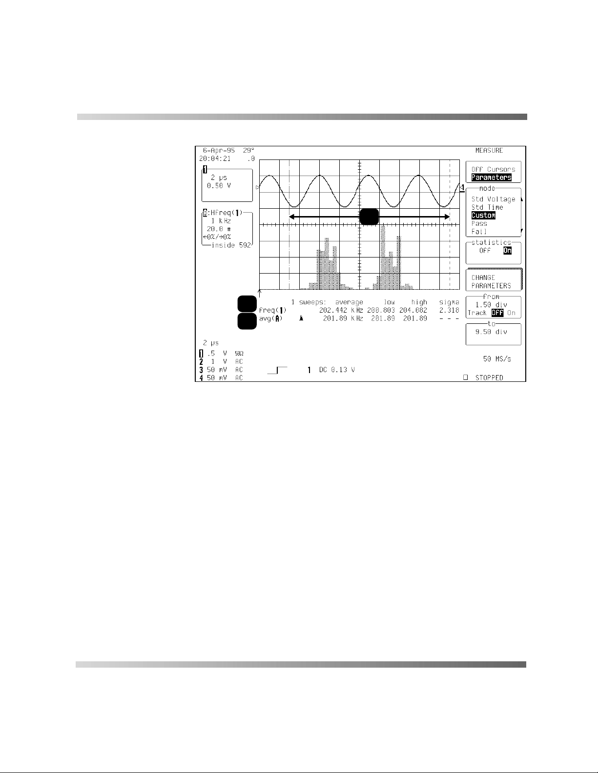
The “MEASURE” “Parameters” menu is accessed by pressing
the CURSORS/MEASURE button, then selecting “Parameters”
from the top menu that appears, as shown in
Figure 1.1
.
Parameters are used to perform waveform measurements for
the section of waveform that lies between the parameter cur sors
(Annotation ➊ in this figure). The position of the parameter
cursors is set using the “from” and “to” m enus and controlled by
the associated ‘menu’ knobs.
The top trace in
parameter measurement is being performed on the waveform
(Annotation ➋) with a value of 202.442 kHz as the average
frequency. The bottom trace shows a histogram of the freq
parameter with an average frequency of 201.89 kHz (Annotation
➌), which is the average frequency of the data contained within
the parameter cursors.
Figure 1.1
shows a sine waveform. A freq
²
Page 6
,QWURGXFWLRQ
1
2
3
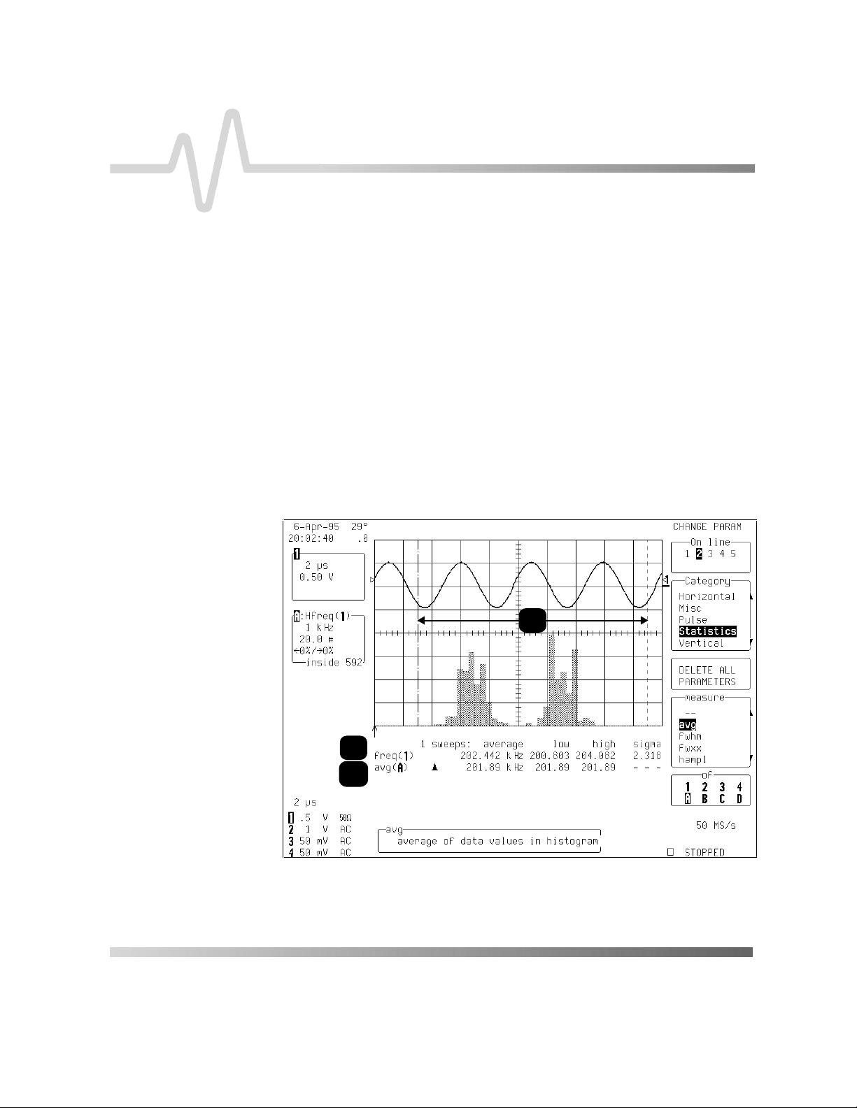
Figure 1.1
Selection of “Custom” from the “mode” menu and then
“CHANGE PARAMETERS” displays the “CHANGE PARAM”
menu group, shown in
can be selected, with each displayed on its own line below the
waveform display grid. Parameter m easurements can then also
be selected from “Category” and “measure” using the
corresponding menu buttons.
Categories are provided for related groups of parameter
measurements. The “Statistics” category is provided for
selection of histogram parameters. After s election of a category,
a parameter can be selected from the “measure” menu.
Selection of parameters is done using the menu buttons or
knobs.
²
Figure 1.2
. Now, up to five parameters
Page 7
:3
The parameter display line is selected from the “On line” menu.
In
Figure 1.2
À The freq measure param eter from the “Cyclic” category for
Trace 1, which had earlier been selected, is displayed on
Line 1 as freq() (
À The avg m easure parameter from the “ Statistics” category
for Trace A is selected for display on Line 2. The avg
parameter provides the mean value of the underlying
measurements for the Trace A histogram section within the
parameter cursors (
Annotation
(
À No parameters have been selected for Lines 3–5.
:
➌
).
Annotation
Annotation
➊
) .
➋
), shown as “avg($)”,
2
1
3
Figure 1.2
²
Page 8

3DUDPHWHU9DOXH
&DOFXODWLRQDQG'LVSOD\
,QWURGXFWLRQ
If a parameter has additional settings that must be supplied in
order to perform measurements, the “MORE ‘xxxx’ SETUP”
menu appears. But if no additional settings are required the
“DELETE ALL PARAMETERS” menu appears , as shown in the
figure above, and pressing the associated menu button res ults in
all five lines of parameters being cleared.
not
When Persistence is
channels shows the captured waveform of a single sweep.
For non-segmented waveforms, the display is identical to a single
acquisition. But with segmented waveform s, the res ult of a single
acquisition for all segments is displayed.
The value displayed for a chosen param eter depends on whether
“statistics” is “On”. And on whether the waveform is segm ented.
These two factors and the param eter chosen determ ine whether
results are provided for a single acquisition (trigger) or multiple
acquisitions. In any case, only the waveform sec tion between the
parameter cursors is used.
If the waveform sourc e is a memory (“M1”, “M2”, “M3” or “M4”)
then loading a new waveform into mem ory acts as a trigger and
sweep. This is also the case when the waveform source is a
zoom of an input channel, and when a new segment or the “All
Segments” menu is selected.
being used, the display for input
When “statistics” is “Off”, the parameter results for the last
acquisition are displayed. This corres ponds to results for the last
segment for segmented waveform s with all segments displayed.
For zoom traces of segmented waveforms, selection of an
individual segment gives the parameter value for the displayed
portion of the segment between the parameter cur sors . Selection
of “All Segments” provides the parameter results f rom the last
segment in the trace.
not
When “On”, and where the parameter does
waveforms in calc ulating a res ult (∆dly, ∆t@lv), results are shown
for all acquisitions since the CLEAR SWEEPS button was last
pressed. If the parameter uses two waveforms, the result of
comparing only the last segment per s weep for eac h waveform
contributes to the statistics.
The statistics for the selected segm ent are displayed for zoom
traces of segm ented waveforms. Selection of a new segment or
²
use two
Page 9

:3
“All Segments” acts as a new sweep and the parameter
calculations for the new segment(s) contribute to the statistics.
Depending on the parameter, single or multiple c alculations can
be performed for each acquisition. For example, the period
parameter calculates a per iod value for each of up to the first 50
cycles in an acquisition. When multiple calculations are
performed, with “ statistics” “Off” the parameter result shows the
average value of these calculations. W hereas “On” displays the
average, low, high and sigma values of all the calculations.
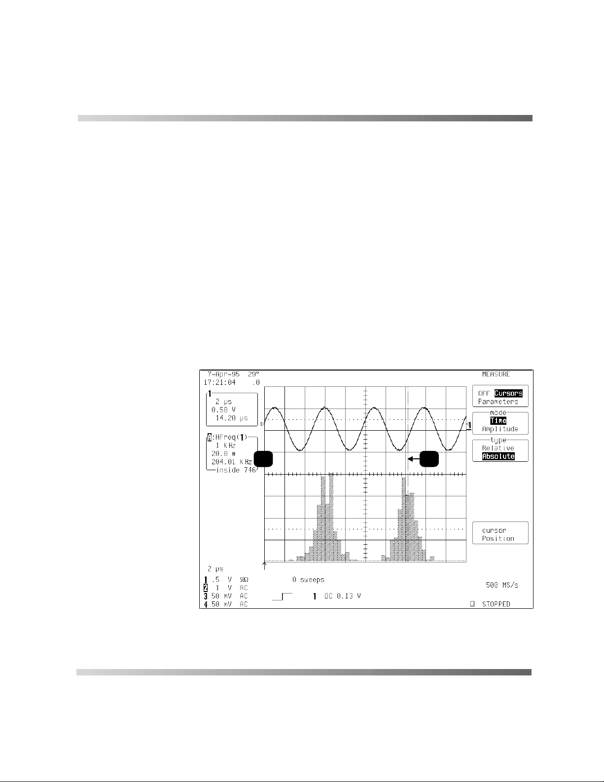
([DPSOH In
signal. The initial impression given the viewer is of some
frequency drift in the signal source. The lower trace shows a
histogram of the frequency as measured by the oscilloscope.
Figure 1.3
, the upper trace shows the persistence display of a
²
Figure 1.3
Page 10
,QWURGXFWLRQ
This histogram indicates two frequency distributions with
dominant frequencies separated by 4000 Hz. There are two
distinct and normal looking distributions, without wide variation,
within each of the two. We can conclude that there are two
dominant frequencies. If the problem were related to frequency
drift, the distribution would have a tendency to be broader, non-
not
normal in appearance, and normally there would
distinct distributions.
After a brief visual analysis, the measurement cursors and
statistical parameters can be used to determine additional
characteristics of distribution, including the most common
frequency in each distribution and the spread of each distribution.
Figure 1.4
Annotation
(
bin of the distribution. The value of the bin, ins ide the Displayed
Trace Field (
Annotation
by
, below, shows the use of the measurement cursor
➊
), to determine the frequency represented by one
see Chapter 2 for a detailed description
➋
.
be two
) is indicated
²
12
Figure 1.4
Page 11

:3
Figure 1.5
Annotations
(
the distribution located between the cursors. The average value
of the measurem ents in the right-hand dis tribution is indicated by
Annotation
3
, below, shows the use of the parameter cursors
➊
and ➋) in determining the average frequenc y of
➌
.
2
1
²
Figure 1.5
Page 12

,QWURGXFWLRQ
Finally,
(
between a bin in the center of each distribution. The value in
k Hz, in the Displayed Trace Field, is indicated by
Figure 1.6
Annotations
3
1
shows the use of the measurement cursors
➊
and ➋) in determining the differ ence in frequenc y
Annotation
2
➌
.
²
Figure 1.6
Page 13

2
Theory of Operation
A statistical understanding of variations in parameter
values is of great interest for many waveform parameter
measurements. Knowledge of the average, minimum,
maximum and standard deviation of the parameter may
often be enough for the user, but in many other instances a
more detailed understanding of the distribution of a
parameter’s values is desired.
Histograms provide the ability to see how a parameter’s values
are distributed over many measurements, enabling this detailed
analysis. They divide a range of parameter values into subranges called bins. Maintained for each bin is a count of the
number of parameter values calculated — events — that fall
within its sub-range.
While the range can be infinite, for practical purposes it need
only be defined as large enough to include any realistically
possible parameter value. For example, in measuring TTL highvoltage values a range of ± 50 V is unnecessarily large, whereas
one of 4 V ± 2.5 V is more reasonable. It is this 5 V range that is
subdivided into bins. And if the number of bins used were 50,
each would have a sub-range of 5 V/50 bins or 0.1 V/bin. Events
falling into the first bin would then be between 1.5 V and 1.6 V.
While the next bin would capture all events between 1.6 V and
1.7 V. And so on.
WP03: Histograms
After a process of several thousand events, the graph of the
count for each bin — its histogram — provides a good
understanding of the distribution of values. Histograms generally
use the ‘x’ axis to show a bin’s sub-range value, and the ‘y’ axis
for the count of parameter values within each bin. The leftmost
bin with a non-zero count shows the lowest parameter value
measurement(s). The vertically highest bin shows the greatest
number of events falling within its sub-range.
The number of events in a bin, peak or a histogram is referred to
its population. Figure 2.1 shows a histogram’s highest population
bin as the one with a sub-range of 4.3–4.4 V — to be expected
of a TTL signal. The lowest value bin with events is that with a
2––1
Page 14
WP03
sub-range of 3.0–3.1 V. As TTL high v oltages need to be greater
than 2.5 V, the lowest bin is within the allowable tolerance.
However, because of its proximity to this tolerance and the
degree of the bin’s separation from all other values, additional
investigation may be desirable.
LeCroy DSO Process LeCroy digital oscilloscopes generate histograms of the
parameter values of input waveforms. But first, the following
must be defined:
¾ The parameter to be histogrammed.
¾ The trace on which the histogram will be displayed.
¾ The maximum number of parameter measurement values to
be used in creating the histogram.
¾ The measurement range of the histogram.
¾ The number of bins to be used.
Once these are defined, the oscilloscope is ready to make the
histogram.
Count
40
30
20
10
1.5
2
3
3.15
Range
4.35
4
5
6
Volts
Figure 2.1
2––2
Page 15

Histograms
The sequence for acquiring histogram data is:
1. trigger
2. waveform acquisition
3. parameter calculation(s)
4. histogram update
5. trigger re-arm.
If the timebase is set in non-segmented mode, a single
acquisition occurs prior to parameter calculations. However, in
Sequence mode an acquisition for each segment occurs prior to
parameter calculations. If the source of histogram data is a
memory, storing new data to memory effectively acts as a
trigger and acquisition. Because updating the screen can take
significant processing time, it occurs only once a second,
minimizing trigger dead-time (under remote control the display
can be turned off to maximize measurement speed).
Parameter Buffer The oscilloscope maintains a circular parameter buffer of the
last
20 000 measurements made, including values that fall outside
the set histogram range. If the maximum number of events to be
used in a histogram is a number ‘N’ less than 20 000, the
histogram will be continuously updated with the last ‘N’ events
as new acquisitions occur. If the maximum number is greater
than 20 000, the histogram will be updated until the number of
events is equal to ‘N’. Then, if the number of bins or the
histogram range is modified, the scope will use the parameter
buffer values to redraw the histogram with either the last ‘N’ or
20 000 values acquired — whichever is the lesser. The
parameter buffer thereby allows histograms to be redisplayed
using an acquired set of values and settings that produce a
distribution shape with the most useful information.
2––3
Page 16

WP03
In many cases the optimal range is not readily apparent. So the
scope has a powerful range-finding function. If required it will
examine the values in the parameter buffer to calculate an
optimal range and redisplay the histogram using it. The
instrument will also give a running count of the number of
parameter values that fall within, below and above the range. If
any fall below or above the range, the range-finder can then
recalculate to include these parameter values, as long as they
are still within the buffer.
Parameter Events Capture The number of events captured per waveform acquisition or
display sweep depends on the parameter type. Acquisitions are
initiated by the occurrence of a trigger event. Sweeps are
equivalent to the waveform captured and displayed on an input
channel (1, 2, 3 or 4). For non-segmented waveforms an
acquisition is identical to a sweep. Whereas for segmented
waveforms an acquisition occurs for each segment and a sweep
is equivalent to acquisitions for all segments. Only the section of
a waveform between the parameter cursors is used in the
calculation of parameter values and corresponding histogram
events.
The following table provides, for each parameter and for a
waveform section between the parameter cursors, a summary of
the number of histogram events captured per acquisition or
sweep.
2––4
Page 17

Histograms
Parameters
(plus others, depending on options)
data All data values in the region analyzed.
duty, freq, period, width, Up to 49 events per acquisition.
ampl, area, base, cmean, cmedian, crms,
csdev, cycles, delay, dur, first, last, maximum,
mean, median, minimum, nbph, nbpw, over+,
over–, phase, pkpk, points, rms, sdev, ∆dly,
∆t@lv
f@level, f80–20%, fall, r@level, r20–80%, rise Up to 49 events per acquisition.
Histogram Parameters Once a histogram is defined and generated, measurements can
be performed on the histogram itself. Typical of these are the
histogram’s:
Number of Events Captured
One event per acquisition.
¾ Average value, standard deviation
¾ Most common value (parameter value of highest count bin)
¾ Leftmost bin position (representing the lowest measured
waveform parameter value)
¾ Rightmost bin (representing the highest measured waveform
parameter value).
Histogram parameters are provided to enable these
measurements. Available through selecting “Statistics”from the
“Category” menu, they are calculated for the selected section
between the parameter cursors (for a full description of each
parameter, see Chapter 3):
2––5
Page 18

WP03
All Segments
avg average of data values in histogram
fwhm full width (of largest peak) at half the maximum bin
fwxx full width (of largest peak) at xx% the maximum bin
hampl histogram amplitude between two largest peaks
hbase histogram base or leftmost of two largest peaks
high highest data value in histogram
hmedian median data value of histogram
hrms rms value of data in histogram
htop histogram top or rightmost of two largest peaks
low lowest data value in histogram
maxp population of most populated bin in histogram
mode data value of most populated bin in histogram
pctl data value in histogram for which specified ‘x’% of
population is smaller
pks number of peaks in histogram
range difference between highest and lowest data values
sigma standard deviation of the data values in histogram
totp total population in histogram
xapk x-axis position of specified largest peak.
Zoom Traces and
Segmented Waveforms
Histogram Peaks Because the shape of histogram distributions is particularly
Example
Histograms of zoom traces display all events for the displayed
portion of a waveform between the parameter cursors. When
dealing with segmented waveforms, and when a single
segment is selected, the histogram will be recalculated for all
events in the displayed portion of this segment between the
parameter cursors. But if “
histogram for all segments will be displayed.
interesting, additional parameter measurements are available
for analyzing these distributions. They are generally centered
around one of several peak value bins, known — together with
its associated bins — as a histogram peak.
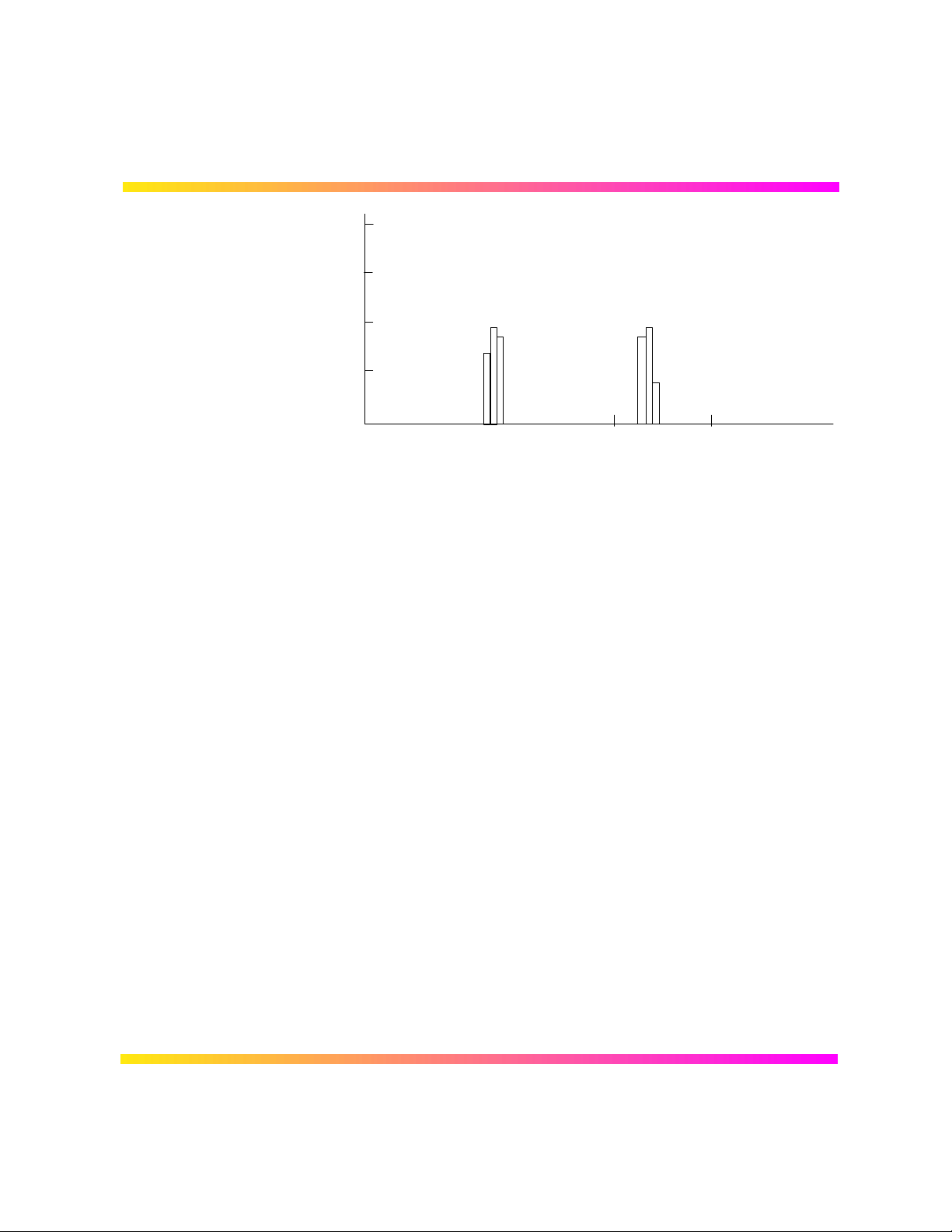
In Figure 2.2, a histogram of the voltage value of a five-volt
amplitude square wave is centered around two peak value bins:
0 V and 5 V. The adjacent bins signify variation due to noise.
The graph of the centered bins shows both as peaks.
2––6
” is selected, the
Page 19
Histograms
Volts
0
Figure 2.2
Determining such peaks is very useful, as they indicate
dominant values of a signal.
However, signal noise and the use of a high number of bins
relative to the number of parameter values acquired, can give a
jagged and spiky histogram, making meaningful peaks hard to
distinguish. The scope analyzes histogram data to identify peaks
from background noise and histogram definition artifacts such as
small gaps, which are due to very narrow bins.
5
Binning and
Measurement
Accuracy
For a detailed description on how the scope determines peaks see
the pks parameter description, Chapter 3.
Histogram bins represent a sub-range of waveform parameter
values, or events. The events represented by a bin may have a
value anywhere within its sub-range. However, parameter
measurements of the histogram itself, such as average, assume
that all events in a bin have a single value. The scope uses the
center value of each bin’s sub-range in all its calculations. The
greater the number of bins used to subdivide a histogram’s
range, the less the potential deviation between actual event
values and those values assumed in histogram parameter
calculations.
Nevertheless, using more bins may require performance of a
greater number of waveform parameter measurements, in order
to populate the bins sufficiently for the identification of a
2––7
Page 20

WP03
characteristic histogram distribution.
In addition, very fine-grained binning will result in gaps between
populated bins that may make determination of peaks difficult.
Figure 2.3 shows a histogram display of 3672 parameter
measurements divided into 2000 bins. The standard deviation of
the histogram sigma (Annotation ) is 81.17 mV. Note the
histogram’s jagged appearance.
1
Figure 2.3
The oscilloscope’s 20 000-parameter buffer is very effective for
determining the optimal number of bins to be used. An optimal
bin number is one where the change in parameter values is
insignificant, and the histogram distribution does not have a
jagged appearance. W ith this buffer, a histogram can be
dynamically redisplayed as the number of bins is modified by
the user. In addition, depending on the number of bins selected,
the change in waveform parameter values can be seen.
2––8
Page 21

Histograms
In Figure 2.4 the histogram shown in the previous figure has
been recalculated with 100 bins. Note how it has become far
less jagged, while the real peaks are more apparent. Also, the
change in sigma is minimal (81.17 mV vs 81 mV).
2––9
Figure 2.4
Page 22

Creating and Analyzing Histograms
5
Annotation
The following provides a description of the oscilloscope’s
operational features for defining, using and analyzing
histograms. The sequence of steps is typical of this
process.
WP03
Selecting the Histogram
Function
Histograms are created by graphing a series of waveform
parameter measurements. The first step is to define the
waveform parameter to be histogrammed. Figure 2.
screen display accompanying the selection of a frequency (freq)
parameter measurement (
Channel 1.
) for a sine waveform on
shows a
1
Figure 2.5
2––10
Page 23

Histograms
The preceding figure shows four waveform cycles, which will
provide four freq parameter values for each histogram, each
sweep. With a freq parameter selected, a histogram based on it
can be specified.
But first the waveform trace must be defined as a histogram.
This is done by pressing the MATH SETUP button. Figure 2.6
shows the resulting display. To place the histogram on Trace A,
the menu button corresponding to the “REDEFINE A” menu is
pressed.
2––11
Figure 2.6
Page 24

WP03
Once a trace is selected, the screen shown in Figure 2.7
appears. Selecting “Yes” from the “use Math?” menu enables
mathematical functions, including histograms.
Figure 2.7
Histogram Trace Setup MenuFigure 2.8 (next page) shows the display when “Histogram”is
selected from the “Math Type” menu. Here, the freq parameter
only has been defined. However, if additional parameters were
to be defined, the individual parameter would need to be
selected — by pressing the corresponding menu button or
turning the associated knob until the desired parameter
appeared in the “Histogram custom line” menu.
2––12
Page 25

Histograms
Figure 2.8
Each time a waveform parameter value is calculated it can be
placed in a histogram bin. The maximum number of such values
is selected from the “using up to” menu. Pressing the
associated menu button or turning the knob allows the user to
select a range from 20 to 2 billion parameter value calculations
for histogram display.
To see the histogram, turn the trace display on by pressing the
appropriate TRACE ON/OFF button, for a display similar that
shown in Figure 2.9.
2––13
Page 26

WP03
1
2
Figure 2.9
Each histogram is set by the user to capture parameter values
falling within a specified range. As the scope captures the
values in this range the bin counts increase. Values not falling
within the range are not used in creating the histogram.
Information on the histogram is provided in the Displayed
Trace Field (Annotation ) for the selected trace. This shows:
¾ The current horizontal per division setting for the histogram
(“1 Hz” in this example). The unit type used is determined by
the waveform parameter type on which the histogram is
based.
¾ The vertical scale in #bin counts per division (here, “200
m”).
¾ The number of parameter values that fall within the range
(“inside 0”)
¾ The percentage that fall below (“←0%”)
2––14
Page 27

Histograms
¾ The percentage of values above the range (“100%→”).
This figure shows that 100% of the captured events are above
the range of bin values set for the histogram. As a result, the
baseline of the histogram graph (Annotation ) is displayed, but
no values appear.
Selecting the “FIND CENTER AND WIDTH” menu allows
calculation of the optimal center and bin-width values, based on
the up to the most recent parameter values calculated. The
number of parameter calculations is chosen with the “using up
to” menu (or 20 000 values if this is greater than 20 000).
Figure 2.10 shows a typical result.
2––15
1
Figure 2.10
Page 28

WP03
If the trace on which the histogram is made is not a zoom, then
all bins with events will be displayed. Otherwise, press RESET
to reset the trace and display all histogram events.
The Information Window (Annotation ) at the bottom of the
previous screen shows a histogram of the freq parameter for
Channel 1 (designated as “A:Hfreq(1)”) for Trace A. The “1000
→ 100 pts” in the window indicates that the signal on Channel 1
has 1000 waveform acquisition samples per sweep and is being
mapped into 100 histogram bins.
Selecting “MORE HIST SETUP” allows additional histogram
settings to be specified, resulting in a display similar to that of
Figure 2.11, below.
2––16
Figure 2.11
Page 29

Histograms
Setting Binning &
Histogram Scale
The “Setup” menu allows modifcation of either the “Binning” or
the histogram “Scale” settings. If “Binning” is selected, the
“classify into” menu appears, as shown in the figure above.
The number of bins used can be set from a range of 20–2000 in
a 1–2–5 sequence, by pressing the corresponding menu button
or turning the associated knob.
If “Scale” is selected from the “Setup” menu, a screen similar
that of Figure 2.12 will be displayed.
2––17
Figure 2.12
Page 30

WP03
Three options are offered by the “vertical” menu for setting the
vertical scale:
1. “Linear” sets the vertical scale as linear (see previous
figure). The baseline of the histogram designates a bin value
of 0. As the bin counts increase beyond that which can be
displayed on screen using the current vertical scale, this
scale is automatically increased in a 1–2–5 sequence.
2. “Log” sets the vertical scale as logarithmic (Fig. 2.13).
Because a value of ‘0’ cannot be specified logarithmically,
no baseline is provided.
2––18
Figure 2.13
Page 31

Histograms
3. “LinConstMax” sets the vertical scaling to a linear value
that uses close to the full vertical display capability of the
scope (Fig. 2.14). The height of the histogram will remain
almost constant.
3
2
1
Figure 2.14
For any of these options, the scope automatically increases the
vertical scale setting as required, ensuring the highest histogram
bin does not exceed the vertical screen display limit.
The “Center” and “Width” menus allow specification of the
histogram center value and width per division. The width per
division times the number of horizontal display divisions (10)
determines the range of parameter values centered on the
number in the “Center” menu, used to create the histogram.
2––19
Page 32

WP03
In the previous figure, the width per division is 2.000 × 10
(Annotation ). As the histogram is of a frequency parameter,
the measurement parameter is hertz.
The range of parameter values contained in the histogram is
therefore:
( 2 k Hz/division) x (10 divisions) = 20 k Hz
with a center of 2.02 E+05 Hz ().
In this example, all freq parameter values within 202 k Hz ± 10
k Hz — from 192 k Hz to 212 k Hz — are used in creating the
histogram. The range is subdivided by the number of bins set by
the user. Here, the range is 20 k Hz, as calculated above, and
the number of bins 100. Therefore, the range of each bin is:
20 k Hz / 100 bins, or
.2 k Hz per bin.
The “Center” menu allows the user to modify the center value’s
mantissa (here, 2.02), exponent (E+05) or the number of digits
used in specifying the mantissa (three). The display scale of
1 k Hz/division, shown in the Trace Display Field, is indicated by
Annotation . This scale has been set using the horizontal zoom
control and can be used to expand the scale for visual
examination of the histogram trace.
3
The use of zoom in this way does not modify the range of data
acquisition for the histogram, only the display scale. The range
of measurement acquisition for the histogram remains based on
the center and width scale, resulting in a range of 202 k Hz ±
10 k Hz for data acquisition.
Any of these can be changed using the associated knob. And
the width/division can be incremented in a 1–2–5 sequence by
selecting “Width”, using button or knob.
Histogram Parameters Once the histogram settings are defined, selecting additional
parameter values is often useful for measuring particular
attributes of the histogram.
2––20
Page 33

Histograms
Selecting “PARAMETER SETUP”, as shown in the previous
figure, accesses the “CHANGE PARAM” menus, shown in
Figure 2.15.
1
Figure 2.15
New parameters can now be selected or previous ones modified. In
this figure, the histogram parameters maxp and mode (Annotation
) have been selected. These determine the count for the bin with
the highest peak, and the corresponding horizontal axis value of that
bin’s center.
Note that both “maxp” and “mode” are followed by “(A)” on the
display. This designates the measurements as being made on
the signal on Trace A, in this case the histogram. Note:
¾ The value of “maxp(A)” is “110 #”, indicating the highest bin
has a count of 110 events.
¾ The value of mode(A) is “203.90 k Hz”, indicating that this
bin is at 203.90 k Hz.
2––21
Page 34

WP03
¾ The icon to the left of “mode” and “maxp” parameters
indicates that the parameter is being made on a trace
defined as a histogram.
However, if these parameters were inadvertently set for a trace
with no histogram they would show ‘---’.
Using Measurement Cursors The parameter cursors can be used to select a section of a
histogram for which a histogram parameter is to be calculated.
Figure 2.16 shows the average, “avg(A)”(Annotation ) of the
distribution between the parameter cursors for a histogram of
the frequency (“freq”) parameter of a waveform. The parameter
cursors () are set “from” 4.70 divisions ()“to” 9.20 divisions
() of the display.
2––22
2
3
1
4
Figure 2.16
Page 35

Histograms
It is recommended that this capability be used only after the
input waveform acquisition has been completed. Otherwise, the
parameter cursors will also select the portion of the input
waveform used to calculate the parameter during acquisition.
This will create a histogram with only the local parameter values
for the selected waveform portion.
Zoom Traces and
Segmented Waveforms
Histograms can also be displayed for traces that are zooms of
segmented waveforms. When a segment from a zoomed trace
is selected, the histogram for that segment will appear. Only the
portion of the segment displayed and between the parameter
cursors will be used in creating the histogram. The
corresponding Displayed Trace Field will show the number of
events captured for the segment.
Figure 2.17 shows “Selected” a histogram of the frequency
(“freq”) parameter for “Segment 1”(Annotation ) of Trace “A”,
which is a zoom of a 10-segment waveform on Channel 1.
2
1
Figure 2.17
The Displayed Trace Field shows that 24 parameter events
(Annotation ) have been captured into the histogram. The
2––23
Page 36

WP03
average value for the freq parameter is displayed as the
histogram parameter, “avg(B)”.
Figure 2.18 shows the result of selecting “All Segments”.
Figure 2.18
Note that the Displayed Trace Field indicates 30 events in the
histogram for all segments, and the change in “avg(B)” .
Histogram events can be cleared at any time by pushing the
CLEAR SWEEPS button. All events in the 20-k parameter
buffer are cleared at the same time. The vertical and horizontal
POSITION and ZOOM control knobs can be used to expand and
position the histogram for zooming-in on a particular feature of
it. The resulting vertical and horizontal scale settings are shown
in the Displayed Trace Field. However, the values in the
“Center” and “Width” menus do not change, since they
2––24
Page 37

Histograms
determine the range of the histogram and cannot be used to
determine the parameter value range of a particular bin. If the
histogram is repositioned using the horizontal POSITION knob
the histogram’s center will be moved from the center of the
screen. Horizontal measurements will then require the use of
CURSORS/MEASURE.
The scope’s measurement cursors are useful for determining the
value and population of selected bins. Figure 2.19 shows the
“Time”cursor () positioned on a selected histogram bin. The
value of the bin () and the population of the bin () are also
shown.
3
1
4
2
Figure 2.19
A histogram’s range is represented by the horizontal width of the
histogram baseline. As the histogram is repositioned vertically
the left and right sides of the baseline can be seen. In this final
figure of the chapter, the left edge of the range is visible ().
2––25
Page 38

:3+LVWRJUDP3DUDPHWHUV
DYJ $YHUDJH
'HILQLWLRQ Average or mean value of data in a histogram.
'HVFULSWLRQ The average is calculated by the formula:
([DPSOH
n
avg =
where n is the number of bins in the his togram , bin count is the count or
height of a bin, and bin value is the center value of the range of
parameter values a bin can represent.
Count#
3.5
3.0
2.5
2.0
1.5
1.0
0.5
(bin count) (bin value) (bin count) ii i
i1
n
/
∑∑
i==
1
,
0
4.0 4.2
The average value of this histogram is:
( 4.1 * 2 + 4.3 * 3 + 4.4 * 1) / 6 = 4.25.
4.1
²
4.3 4.4
V al ue (vo l t s)
Page 39

:3
IZKP )XOO:LGWKDW+DOI0D[LPXP
'HILQLWLRQ Determines the width of the largest area peak , measured between bins
on either side of the highest bin in the peak that have a population of
half the highest’s population. If several peak s have an area equal to the
maximum population, the leftmost peak is used in the computation.
'HVFULSWLRQ First, the highest population peak is identified and the height of its
highest bin (population) determined (
determined see the pks parameter description
bins to the right and left are found, until a bin on each side is found to
have a population of less than 50% of that of the highest bin’s. A line is
calculated on each side, from the c enter point of the first bin below the
50% population to that of the adjacent bin, towards the highes t bin. The
intersection points of these lines with the 50% height value is then
determined. The length of a line c onnecting the inters ection points is the
value for fwhm.
for a discussion on how peaks are
). Next, the populations of
([DPSOH
12
maximum
10
8
7
6
50% maximum
4
3
2
1
fwhm
5
3
²
Page 40

+LVWRJUDP3DUDPHWHUV
IZ[[ )XOO:LGWKDW[[0D[LPXP
'HILQLWLRQ Determines the width of the largest ar ea peak, measured between bins
on either side of the highest bin in the peak that have a population of
xx% of the highest’s population. If several peaks have an ar ea equal to
the maximum population, the leftmost peak is used in the computation.
'HVFULSWLRQ First, the highest population peak is identified and the height of its
highest bin (population) determined (
see the pks description
bin populations to the right and left are found until a bin on each side is
found to have a population of less than xx% of that of the highes t bin. A
line is calculated on each side, from the center point of the first bin
below the 50% population to that of the adjacent bin, towards the
highest bin. The intersection points of these lines with the xx% height
value is then determined. The length of a line connecting the intersection
points is the value for fwxx.
3DUDPHWHU6HWWLQJV Selection of the fwxx parameter in the “CHANGE PARAM” m enu group
causes the “MORE fwxx SETUP” menu to appear. Pressing the
corresponding menu button displays a threshold setting menu that
enables the user to set the ‘xx’ value to between 0–100% of the peak.
). Next, the
([DPSOH fwxx with threshold set to 35%:
12
maximum
3
35% maximu m
2
1
²
10
8
7
6
5
4
3
fwhm
Page 41

:3
peak #2
KDPSO +LVWRJUDP$PSOLWXGH
'HILQLWLRQ The differenc e in value of the two mos t populated peaks in a his togram .
This parameter is useful for waveforms with two primary parameter
values, such as TTL voltages, where hampl would indicate the
difference between the binary ‘1’ and ‘0’ voltage values.
'HVFULSWLRQ The values at the center (line dividing the population of peak in half) of
([DPSOH
the two highest peaks are determined (
The value of the leftmost of the two peaks is the histogram base (
hbase). W hile that of the rightm os t is the histogr am top (
parameter is then calculated as:
hampl = htop − hbase
see pks parameter description
see
htop). The
).
see
peak #1
152150
hampl
base
In this histogram, hampl is 152 mV − 150 mV = 2 mV.
²
top
Page 42

+LVWRJUDP3DUDPHWHUV
+EDVH +LVWRJUDP%DVH
'HILQLWLRQ The value of the leftmost of the two most populated peaks in a
histogram. This parameter is primarily useful for waveforms with two
primary parameter values such as TTL voltages where hbase would
indicate the binary ‘0’ voltage value.
'HVFULSWLRQ The two highest histogram peaks are determined. If several peaks are
([DPSOH
of equal height the leftmost peak am ong these is used (
the leftmost of the two identif ied peaks is selected. This peak ’s center
value (line that divides population of peak in half) is the hbase.
see pks
). Then
peak #1
150
hbase
peak #2
²
Page 43

:3
KLJK +LJK
'HILQLWLRQ The value of the rightmost populated bin in a histogram.
'HVFULSWLRQ The rightm ost of all populated histogram bins is determ ined: high is its
center value, the highest parameter value shown in the histogram.
([DPSOH
count
In this histogram high is 152 mV.
²
152
high
mV
Page 44

+LVWRJUDP3DUDPHWHUV
KPHGLDQ +LVWRJUDP0HGLDQ
'HILQLWLRQ The value of the ‘x’ axis of a histogram, dividing the histogram
population into two equal halves.
'HVFULSWLRQ The total population of the histogram is determ ined. Scanning from left
to right, the population of each bin is summ ed until a bin that causes the
sum to equal or exceed half the population value is encountered. The
proportion of the population of the bin needed for a sum of half the total
population is then determined. Using this propor tion, the horizontal value
of the bin at the same proportion of its range is found, and returned as
hmedian.
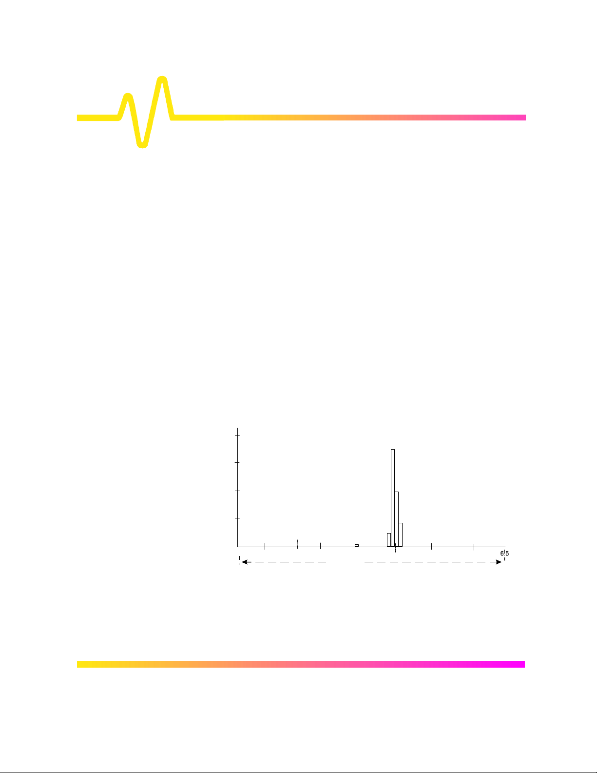
([DPSOH The total population of a histogram is 100 and the histogram range is
divided into 20 bins. The population sum, f rom left to right, is 48 at the
eighth bin. The population of the ninth bin is 8 and its sub-range is f rom
6.1–6.5 V. The ratio of counts needed for half- to total-bin population is:
2 counts needed / 8 counts = .25
The value for hmedian is:
6.1 volts + .25 * (6.5 − 6.1) volts = 6.2 volts
²
Page 45

:3
KUPV +LVWRJUDP5RRW0HDQ6TXDUH
'HILQLWLRQ The rms value of the values in a histogram.
'HVFULSWLRQ The center value of each populated bin is squared and m ultiplied by the
population (height) of the bin. All results are summed and the total is
divided by the population of all the bins. The square root of the result is
returned as hrms.
([DPSOH Using the histogram shown here, the value for hrms is:
22
count
hrms =
(3.5 * 2 + 2.5 * 4)/6
= 2.87
4
3
2
1
2.5 3.5
²
value
Page 46

+LVWRJUDP3DUDPHWHUV
KWRS +LVWRJUDP7RS
'HILQLWLRQ The value of the rightmost of the two most populated peaks in a
histogram. This parameter is useful for waveforms with two primary
parameter values, such as T TL voltages , where htop would indicate the
binary ‘1’ voltage value.
'HVFULSWLRQ The two highest histogram peaks are determ ined. The rightmost of the
two identified peaks is then selected. The center of that peak is htop
(center is the horizontal point where the population to the left is equal to
the area to the right).
([DPSOH
peak #1
²
peak #2
152
htop
mV
Page 47

:3
ORZ /RZ
'HILQLWLRQ The value of the leftmost populated bin in a histogram population. It
indicates the lowest parameter value in a histogram’s population.
'HVFULSWLRQ The leftmost of all populated histogram bins is determined. The center
value of that bin is low.
([DPSOH
count
Low
In this histogram low is 140 mV.
²
150 152140
mV
Page 48

+LVWRJUDP3DUDPHWHUV
PD[S 0D[LPXP3RSXODWLRQ
'HILQLWLRQ The count (vertical value) of the highest population bin in a histogram.
'HVFULSWLRQ Each bin between the param eter cursors is ex amined for its count. The
highest count is returned as maxp.
([DPSOH
maxp
In this example, maxp is 14.
²
Page 49

:3
PRGH 0RGH
'HILQLWLRQ The value of the highest population bin in a histogram.
'HVFULSWLRQ Each bin between the parameter cursor s is examined for its population
count. The leftmost bin with the highest count found is selected. Its
center value is returned as mode.
([DPSOH
count
In this example mode is 150 mV.
²
150
mode
mV
Page 50

+LVWRJUDP3DUDPHWHUV
SFWO 3HUFHQWLOH
'HILQLWLRQ Computes the horizontal data value that separates the data in a
histogram, so that the population on the left is a specified percentage
‘xx’ of the total population. W hen the thres hold is set to 50%, pctl is the
same as hmedian.
'HVFULSWLRQ The total population of the histogram is determined. Scanning from lef t
to right, the population of each bin is summ ed until a bin that causes the
sum to equal or exceed ‘xx’% of the population value is encountered. A
ratio of the number of counts needed for ‘xx’% population/total bin
population is then determined for the bin. The horizontal value of the bin
at that ratio point of its range is found, and returned as pctl.
([DPSOH The total population of a histogram is 100. The histogram range is
divided into 20 bins and ‘xx’ is set to 25%. The population sum at the
sixth bin from the lef t is 22. The population of the seventh is 9 and its
sub-range is 6.1–6.4 V. The ratio of counts needed f or 25% population
to total bin population is:
3 counts needed / 9 counts = 1/3.
The value for pctl is:
6.1 volts + .33 * (6.4 − 6.1) volts = 6.2 volts.
3DUDPHWHU6HWWLQJV Selection of the pctl parameter in the “CHANGE PARAM” menu group
causes the “MORE pctl SETUP” menu to appear. Pressing the
correponding menu button displays a threshold setting m enu. And with
the associated knob the user can set the per centage value to between
1% and 100% of the total population.
²
Page 51

:3
SNV 3HDNV
'HILQLWLRQ The number of peaks in a histogram.
'HVFULSWLRQ The instrument analyzes histogram data to identify peaks from
background noise and histogram binning artifacts such as small gaps.
Peak identification is a three-step process:
1) The mean height of the histogram is calculated for all populated
bins. A threshold (T1) is calculated from this mean where:
T1= mean + 2 sqrt(mean).
2) A second threshold is determined based on all populated bins
under T1 in height, where:
T2 = mean + 2 * sigma,
and where sigma is the standard deviation of all populated bins
under T1.
3) Once T2 is defined, the histogram distribution is scanned f rom lef t
to right. Any bin that crosses above T2 signifies the ex istence of a
peak. Scanning continues to the right until one bin or more
crosses below T2. However, if the bin(s) c ross below T2 for less
than a hundreth of the histogram range, they are ignored, and
scanning continues in search of a peak(s) that cross es under T2
for more than a hundreth of the histogram range. Scanning goes
on over the remainder of the range to identify additional peaks.
Additional peaks within a fiftieth of the range of the populated part
of a bin from a previous peak are ignored.
Note: If the number of bins is set too high a histogram may have many
small gaps. This increases sigma and thereby T2, and in extreme cases
can prevent determination of a peak, even if one appears to be present to
the eye.
²
Page 52

+LVWRJUDP3DUDPHWHUV
([DPSOH The example below shows that two peaks have been identified. T he
peak with the highest population is peak #1.
T2
peak #1 peak #2
²
Page 53

:3
UDQJH 5DQJH
'HILQLWLRQ Computes the difference between the value of the rightmos t and that of
the leftmost populated bin.
'HVFULSWLRQ The rightm ost and leftm ost populated bins are identif ied. The difference
in value between the two is returned as the range.
([DPSOH
count
150
In this example range is 2 mV.
²
range
152
mV
Page 54

+LVWRJUDP3DUDPHWHUV
VLJPD 6LJPD
'HILQLWLRQ The standard deviation of the data in a histogram.
'HVFULSWLRQ sigma is calculated by the formulas:
mean =
i1
sigma =
n
[bin count *(bin value - mean) ] [bin count] 1ii
i1
where n is the number of bins in the his togram , bin count is the count or
height of a bin and bin value is the center value of the range of
parameter values a bin can represent.
([DPSOH For the histogram:
Count#
3.5
3.0
2.5
2.0
1.5
∑∑
i1
n
/(
∑∑
==
i1
n
==
;
,
i
−
n
[bin count *bin value] bin countii i
2
/( )
1.0
0.5
0
4.0 4.2
4.1
4.3 4.4
mean = ( 2 * 4.1 + 3* 4.3 + 1 * 4.4) / 6 = 4.25
sigma =
(2 * (4.1 - 4.25) + 3 * (4.3 - 4.25) + 1*(4.4 - 4.25) ) / (6 - 1)
222
²
V a lue (v olt s )
= .1225
Page 55

:3
WRWS 7RWDO3RSXODWLRQ
'HILQLWLRQ Calculates the total population of a histogram between the parameter
cursors.
'HVFULSWLRQ The count for all populated bins between the parameter cursors is
summed.
([DPSOH
5
Count
4
3
2
1
The total population of this histogram is 9.
²
Page 56

+LVWRJUDP3DUDPHWHUV
Largest-area
[DSN ;&RRUGLQDWHRI[[·WK3HDN
'HILQLWLRQ Returns the value of the xx’th peak that is the largest by area in a
histogram.
'HVFULSWLRQ First the peaks in a histogram are determined and ranked in order of
total area (for a discussion on how peaks are identified see the
description for the pks parameter) . The center of the n’th ranked peak
(the point where the area to the left is equal to the area to the right),
where n is selected by the user, is then returned as xapk.
([DPSOH The rightmost peak is the largest, and thus the first-rank ed, in area ( 1).
The leftmost peak, although higher, is r anked second by area (2). The
lowest peak is also the smallest in area (3).
2
²
1
3
peak
Page 57

d
:37UHQGLQJ
9LVXDOL]LQJ7UHQGV
The Trend waveform processing function enables the
creation of graphs of successive waveform parameter
measurement values. It provides useful visual information
on waveform parameter variation. And, used together with
other scope features, it allows the graphing of certain
parameters against others.
7R&RQILJXUHD7UHQG
1. Select and configure a custom parameter, which will be used to perform the
measurement that is to be trended. This can be done by either:
À
choosing “Custom” mode from the “MEASURE” “Parameters” menu group as for
histograms (see page 1–3 of the present manual and the CURSORS/MEASURE &
Parameters chapter of the oscilloscope Operator’s Manual), or
À
accessing the same menu group using the “PARAMETER SETUP” menu from the
“TREND…” group (see following pages).
And then selecting the desired parameter from the “CHANGE PARAM” menus that
will be displayed.
2. Define one of the definable traces — A, B, C or D — as using Math and select “Trend”
as the “Math Type” (see page 4–4).
3. Select the custom parameter line to be used in the trend.
4. Choose the number of values to be placed in the generated trend (page 4–5).
5. Decide whether all the parameters generated from the waveform or only the average
of all parameter calculations for each waveform acquisition should be placed in the
trend.
6. If desired, the center and height of the trend can also be configured at this stage, in
the base units of the parameter being trended. However, this is not a requirement an
“FIND CENTER AND HEIGHT” can be used to center the trend once the trend has
been calculated.
²
Page 58

7KH7UHQG&RQILJXUDWLRQ0HQXV
:3
Press to access the ZOOM + MATH menus (
MATH SETUP
page 1–3 of the present manual
each of the four traces, A, B, C and D and access their “SETUP”
menus.
=2200$7+ — illustrated in this ex ample with Trace A def ined as a trend of the
parameter
zooms of Traces 1 and 2.
5('(),1($
Defined as the trend of the custom parameter, performed on
Channel 1, Trace A can be set up by pressing the button
corresponding to this menu.
5('(),1(%
Defined as the trend of the custom parameter, performed on
Channel 1, Trace B can be set up by pressing the button
corresponding to this menu.
5('(),1(&
Defined as a zoom of Channel 1, Trace C can be set up by pressing
the button corresponding to this menu.
Chapter of the scope
amplitude
and Trace B as a trend of
Operator’s Manual
). These allow the redefinition of
period
see the
and
. C and D are
5('(),1('
Defined as a zoom of Channel 2, Trace D can be set up by pressing
the button corresponding to this menu.
0XOWL=RRP
When “On”, enables zoom and position controls on all traces at
once.
IRU0DWK8VH
To set the number of points in certain math functions, using the
associated menu knob.
²
Page 59

7UHQGLQJ
1RWHIRU'LVSOD\RI7UHQGV
The display of defined traces is controlled by the
À
TRACE ON/OFF buttons.
À
Expansion, or zooming, and positioning of traces is
controlled by the horizontal and vertical ZOOM and
POSITION knobs.
À
When Multi-zoom is on, the ZOOM and POSITION
knobs are coupled and control all displayed traces at
once. This is particularly useful when multiple trends
of related parameters are displayed.
À
The button resets the multiplier for the trace
expansion to ‘1’ and the offset positioning to ‘0’. The
button should be pressed for each reconfigured trace
in order that traces can be cleanly and correctly
positioned on-screen.
²
Page 60

:3
6(7832)$ — allows the selected trace (here, Trace A) to be set up for trending.
XVH0DWK"
To define the trend as using math — necessary for the tren d itse lf to
be defined. Traces can be defined to use m ath or as zoom s of other
traces. As trending is a math func tion, “use Math?” should b e set to
“Yes”, using the corresponding menu button.
0DWK7\SH
For selecting “Trend”.
025(75(1'6(783
To access more trend setup options and the final trend-dedicated
menu (
),1'&(17(5$1'+(,*+7
For positioning the trend automatic ally once it has been calculated.
“FIND CENTER AND HEIGHT” places the trace appropriately,
centering and scaling the trend without affecting the zoom and
position settings. But ensure that t hese setti ngs have b een res et (
next page
described on the previous page
).
as
).
7UHQGRI
To select the param eter for trending, usi ng the corres ponding m enu
button or associated knob. Any of the configured parameters,
displayed on the line beneath the grid, can be chosen.
8VLQJXSWR
For selecting — using button or knob — the number of values in the
trend. A maximum of 20 000 values can be chosen for any one
trend. When this max im um is exc eeded, the par ameter results scroll
off the trend.
²
Page 61

7UHQGLQJ
75(1'$ — this menu group appears when “MORE TREND SETUP” is
selected (previous page).
9DOXHV
To select “All” — for every param eter c alculation o n each wa vefor m
to be placed in the trend. Or “Average” — to trend only the average
of all the given values calculated on a given acquisition, and to
obtain one point in the trend per acquisition. Unless this is
specifically required, “All” should be selected.
3$5$0(7(56(783
To access the setup m enus for the selected parameter, the same
menus as the “CHANGE PARAM” group.
),1'&(17(5$1'+(,*+7
For positioning the trend automatically once calculated. “FIND
CENTER AND HEIGHT” places the trace appropriately, centering
and scaling the trend without affecting the zoom and position
settings. But ensure that these settings have been reset (
described in the panel on page 4–1
).
as
&HQWHU
For selecting the mantissa, exponent or n umber of digits res olution,
using the associated knob. The configuration is the value at the
horizontal center line on the grid, while units are those of the
parameter trended.
+HLJKW
To select — using button or knob — the vertical value of each
vertical screen division. Units are those of the parameter trended.
1RWH
Press after having configured the parameter in
“CHANGE PARAM” to return to the menus shown this page.
²
Page 62

7UHQG&DOFXODWLRQ
Once the trend has been configured, parameter values will be
calculated and trended on each subsequent acquisition.
Immediately following the acquisition, its trend values will be
calculated. The resulting trend is a waveform of data points that
can be used the same way as any other waveform. Parameters
can be calculated on it, and it can zoomed, serve as the
trace in an XY plot, and used in cursor measurements.
The sequence for acquiring trend data is:
1. trigger
2. waveform acquisition
3. parameter calculation(s)
4. trend update
5. trigger re-arm.
If the timebase is set in non- segmented mode, a single acquisition
occurs prior to param eter calculations. However, in segment mode
an acquisition for each segment occurs prior to parameter
calculations. If the source of trend data is a memory, storing new
data to memory effectively acts as a trigger and acquisition. Because
updating the screen can tak e significant processing time, it occurs
only once a second, minimizing trigger dead-time (under remote
control the display can be turned off to maximize measurement
speed).
:3
x
or
y
3DUDPHWHU%XIIHU The oscilloscope maintains a circular parameter buffer of the last
20 000 measurements m ade, including values that fall outsi de the
set trend range. If the m aximum number of events to be used in a
trend is a number ‘N’ less than 20 000, the trend will be continuously
updated with the last ‘N’ events as new acquisitions occur. If the
maximum number is greater than 20 000, the trend will be updat ed
until the number of events is equal to ‘N’. Then, if the number of bins
or the trend range is modified, the scope will use the parameter
buffer values to redraw the trend with either th e last ‘N’ or 20 000
values acquired — whichever is the lesser.
²
Page 63

7UHQGLQJ
The parameter buffer ther eby allows trends to be r edisplayed us ing
an acquired set of values and settings that produce a distribution
shape with the most useful information.
In many cases the optimal range is not readily apparent. So the
scope has a powerful range-finding function. If required it will
examine the values in t he parameter buffer to calculate an optimal
range and redisplay the trend using it. The instrument will also give a
running count of the number of parameter values that fall within,
below and above the range. If any fall below or above the rang e, th e
range-finder can then rec alculat e to include these par ameter values,
as long as they are still within the buffer.
3DUDPHWHU(YHQWV&DSWXUH The number of events c aptured per wavefor m acquisition or displa y
sweep depends on the parameter t ype. Acquisitions are initi ated by
the occurrence of a trigger event. Sweeps are equivalent to the
waveform captured and displayed on an input cha nnel ( 1, 2, 3 or 4) .
For non-segmented waveforms an acquisition is identical to a
sweep. Whereas for segmented waveforms an acquisition occurs for
each segment and a sweep is equivalent to acquisitions for all
segments. Only the section of a wavef orm between the parameter
cursors is used in the calculation of parameter values and
corresponding trend events. T he table provides, for each standard
parameter and for a waveform section between the parameter
cursors, a summary of the number of trend events captured per
acquisition or sweep.
3DUDPHWHUV
(plus others, depending on options)
data
duty, freq, period, width,
ampl, area, base, cmean, cmedian, crms,
csdev, cycles, delay, dur, first, last, maximum,
mean, median, minimum, nbph, nbpw, over+,
over–, phase, pkpk, points, rms, sdev, ∆dly,
∆t@lv
f@level, f80–20%, fall, r@level, r20–80%, rise
1XPEHURI(YHQWV&DSWXUHG
All data values in the region analyzed.
Up to 49 events per acquisition.
One event per acquisition.
Up to 49 events per acquisition.
²
Page 64

:3
n
5HDGLQJ7UHQGV
A trend is like any other waveform: its horizontal axis is in units of
events, with earlier events in the leftmost part of the waveform and later events to the
right. And its vertical axis is in the same units as the trended parameter. When the
$
trend is displayed, trace labels like the ones below — for Trace
in these examples —
appear in their customary place on-screen, identifying the trace, the math function
performed and giving horizontal and vertical informatio
¿
# number of events per horizontal division
¿
Units per vertical division, in uni ts of th e parame ter being measur ed
¿
Vertical value at point in trend at cursor location when using cursors
¿
Number of events in trend that are within unzoomed horizontal
display range.
¿
Percentage of values lying beyond the unzoomed vertical range
when
not
in cursor measurement mode.
…
²
Page 65

7UHQGLQJ
8VLQJ0HDVXUHPHQW&XUVRUV The parameter cur sors can be used to determ ine the value and
population of selected areas.
Figure 4.1
the selected trend vertex, whose order number (➋) and va lue (➌)
are also shown.
shows the Tim e cursors ( Annotation ➊) posi tioned on
1
3
1
2
²
Figure 4.1
Page 66

,QGH[
$
avg parameter, 2–6, 3–1
%
Binning menu, 2–17
&
Center menu, 2–19
classify into menu, 2–17
CLEAR SWEEPS, 1–5
CURSORS MEASURE, 1–1
'
defining for trends, 4–2
DELETE ALL PARAMETERS
menu, 1–5
)
FIND CENTER AND HEIGHT
menu, 4–5
FIND CENTER AND WIDTH
menu, 2–15
from menu, 1–2
fwhm parameter, 2–6, 3–2
fwxx parameter, 2–6, 3–3
*
graphing parameters, 4–1
+
hampl parameter, 2–6, 3–4
hbase parameter, 2–6, 3–5
high parameter, 2–6, 3–6
histograms
binning and measurement
accuracy, 2– 7
clearing events, 2–24
defining waveform
parameters, 2–10
definition, 2–1–2–2
Displayed Trace Field, 1–7,
2–14, 2–24
displaying all captured
events, 2–15
DSO process, 2–2
events, 2–1
histogram parameters, 2–5
histogram peaks, 2–6, 3–14
icon, 2–22
information window, 2–16
list of parameters, 2–5
maximum number of
parameter events used,
2–13
measuring individual bin
values, 2–25
number of parameter events
captured, 2–4
parameter buffer, 2–3
range, 2–1
range display, 2–25
segmented waveforms, 2–4,
2–6, 2–23
selecting number of bins,
2–17
setting optimal number of
bins, 2–8
setting range center and
width, 2–19
statistics category, 2–5
waveform acquisitions and
histograms, 2–3
zoom traces, 2–6, 2–23
hmedian parameter, 2–6, 3–7
hrms parameter, 2–6, 3–8
htop parameter, 2–6, 3–9
/
low parameter, 2–6, 3–10
Page 67

0
Math setup, 4–2
Math Setup, 1–1
MATH SETUP, 2–11
maxp parameter, 2–6, 3–11
MEASURE menu, 1–3
mode menu, 1–3
mode parameter, 2–6, 3–12
MORE ‘xxxx’ SETUP menu,
1–5
More Hist Setup menu, 2–16
Multi-Zoom, 4–2
3
parameter cursors, 1–2
Parameter Setup, 4–5
Parameter Setup menu, 2–21
parameter values
factors affecting, 1–5
segmented waveforms, 1–5
with statistics on, 1–5
Parameter values
in trending, 4–6
parameters
changing, 1–2–1–3
lines of, 1–3
selecting, 1–2–1–3
pct1 parameter, 2–6
pctl parameter, 3–13
pks parameter, 2–6, 3–14
5
range parameter, 2–6, 3–16
REDEFINE A menu, 2–11
REDEFINE menus, 4–2
6
Scale menu, 2–17
setting no. points in math
functions, 4–2
SETUP menu, 2–17
sigma parameter, 2–6, 3–17
Statistics category, 1–3
7
Time cursors, 4–9
to menu, 1–2
totp parameter, 2–6, 3–18
TREND menu, 4–5
trend setup and configuration,
4–2
trends, 4–1
list of parameters, 4–7
number of parameter events
captured, 4–7
parameter buffer, 4–6
segmented waveforms, 4–7
using measurement cursors,
4–9
waveform acquisitions and
histograms, 4–6
8
use Math? menu, 2–12, 4–4
using up to menu, 2–13
:
Width menu, 2–19
;
xapk parameter, 2–6, 3–19
 Loading...