Lecroy WaveSurfer User Manual

WELCOME

Welcome to on-line help. Use this on-line manual for assistance in normal operation of your LeCroy oscilloscope. You can also use it for help
with LeCroy software options that you may have purchased.

Use the Table of Contents or Index at left to find information.

HOW TO USE ON-LINE HELP

A

Type Styles

ctivators of pop-up text and images appear as green, underlined, italic: Pop-up. To close pop-up text and images after opening them, touch

the pop-up text again.

Link text appears blue and underlined: Link
window. After making a jump, you can touch the Back
left. With each touch of the

icon, you return to the preceding Help screen.

Back

. Links jump you to other topics, URLs, or images; or to another location within the same Help

icon in the toolbar at the top of the Help window to return to the Help screen you just

Instrument Help

When you press the front panel
a menu: you can choose either to have information found for you automatically or to search for information yourself.

If you want context-sensitive Help, that is, Help related to what was displayed on the screen when you requested Help, touch

about. The instrument will automatically display Help about that control.

If you want information about something not displayed on the screen, touch one of the buttons inside the drop-down menu to display the on­line Help manual:

Once opened, the Help window will display its navigation pane: the part of the window that shows the Table of Contents and Index. When you
touch anywhere outside of the Help window, this navigation pane will disappear to reveal more of your signal. To make it return, touch the

Show

icon at the top of the Help window or touch inside the Help information pane.

in the drop-down menu, then touch the on-screen control (or front panel button or knob) that you need information

button (if available), or touch the on-screen

ELP

H

Contents

Index

Search

www.LeCroy.com

and other useful information. This feature requires that the instrument be connected to the internet through
the Ethernet port on the scope's rear panel. Refer to Remote Communication

About

displays the Table of Contents.

displays an alphabetical listing of keywords.

locates every occurrence of the keyword that you enter.

connects you to LeCroy's Web site where you can find Lab Briefs, Application Notes,

opens the Utilities "Status" dialog, which shows software version and other system information.

button , you will be presented with

Help

for setup instructions.

Windows Help

In addition to instrument Help, you can also access on-line Help for Microsoft® Windows®. This help is accessible by minimizing the scope
application, then touching the

Top of Page

button in the Windows task bar at the bottom of the screen and selecting

Start

Help

.

RETURNING A PRODUCT FOR SERVICE OR REPAIR

If you need to return a LeCroy product, identify it by its model and serial numbers. Describe the defect or failure, and give us your name and
telephone number.

For factory returns, use a Return Authorization Number (RAN), which you can get from customer service. Write the number clearly on the
outside of the shipping carton.

Return products requiring only maintenance to your local customer service center.

If you need to return your scope for any reason, use the original shipping carton. If this is not possible, be sure to use a rigid carton. The scope
should be packed so that it is surrounded by a minimum of four inches (10 cm) of shock absorbent material.

Within the warranty period, transportation charges to the factory will be your responsibility. Products under warranty will be returned to you
with transport prepaid by LeCroy. Outside the warranty period, you will have to provide us with a purchase order number before the work can
be done. You will be billed for parts and labor related to the repair work, as well as for shipping.

You should prepay return shipments. LeCroy cannot accept COD (Cash On Delivery) or Collect Return shipments. We recommend using air
freight.

Top of Page

TECHNICAL SUPPORT

You can get assistance with installation, calibration, and a full range of software applications from your customer service center. Visit the
LeCroy Web site at http://www.lecroy.com for the center nearest you.

STAYING UP-TO-DATE

To maintain your instrument’s performance within specifications, have us calibrate it at least once a year. LeCroy offers state-of-the-art
performance by continually refining and improving the instrument’s capabilities and operation. We frequently update both firmware and
software during service, free of charge during warranty.

You can also install new purchased software options in your scope yourself, without having to return it to the factory. Simply provide us with
your instrument serial number and ID, and the version number of instrument software installed. We will provide you with a unique option key
that consists of a code to be entered through the Utilities' Options dialog to load the software option.

Top of Page

WARRANTY

The instrument is warranted for normal use and operation, within specifications, for a period of three years from shipment. LeCroy will either
repair or, at our option, replace any product returned to one of our authorized service centers within this period. However, in order to do this
we must first examine the product and find that it is defective due to workmanship or materials and not due to misuse, neglect, accident, or
abnormal conditions or operation.

LeCroy shall not be responsible for any damage caused by improper connection to incompatible equipment, or for any damage or
malfunction caused by the use of non-LeCroy supplies.

Spare and replacement parts, and repairs, all have a 90-day warranty.

The oscilloscope’s firmware has been thoroughly tested and is presumed to be functional. Nevertheless, it is supplied without warranty of any
kind covering detailed performance. Products not made by LeCroy are covered solely by the warranty of the original equipment manufacturer.

Top of Page

COPYRIGHT

© 2004 by LeCroy Corporation. All rights reserved.

LeCroy, ActiveDSO, ProBus, SMART Trigger, JitterTrack, WavePro, and Waverunner are registered trademarks of LeCroy Corporation.
WaveMaster and X-Stream are trademarks of LeCroy Corporation. Information in this publication supersedes all earlier versions.
Specifications subject to change without notice.

LeCroy Corporation
700 Chestnut Ridge Road
Chestnut Ridge, NY 10977-6499

Tel: [phone]
Fax: [phone]

Internet: www.lecroy.com

ISO

9001:2000

FM 65813

Manufactured under an ISO 9000 Registered Quality Management System

Windows License Agreement

LeCroy's agreement with Microsoft prohibits users from running software on LeCroy X-Stream oscilloscopes that is not relevant to measuring,
analyzing, or documenting waveforms.

END-USER LICENSE AGREEMENT FOR LECROY® X-STREAM™ SOFTWARE
IMPORTANT-READ CAREFULLY: THIS END-USER LICENSE AGREEMENT (“EULA”) IS A LEGAL AGREEMENT BETWEEN THE

INDIVIDUAL OR ENTITY LICENSING THE SOFTWARE PRODUCT (“YOU” OR “YOUR”) AND LECROY CORPORATION (“LECROY”)
FOR THE SOFTWARE PRODUCT(S) ACCOMPANYING THIS EULA, WHICH INCLUDE(S): COMPUTER PROGRAMS; ANY “ONLINE”
OR ELECTRONIC DOCUMENTATION AND PRINTED MATERIALS PROVIDED BY LECROY HEREWITH (“DOCUMENTATION”);
ASSOCIATED MEDIA; AND ANY UPDATES (AS DEFINED BELOW) (COLLECTIVELY, THE “SOFTWARE PRODUCT”). BY USING AN
INSTRUMENT TOGETHER WITH OR CONTAINING THE SOFTWARE PRODUCT, OR BY INSTALLING, COPYING, OR OTHERWISE
USING THE SOFTWARE PRODUCT, IN WHOLE OR IN PART, YOU AGREE TO BE BOUND BY THE TERMS OF THIS EULA. IF YOU DO
NOT AGREE TO THE TERMS OF THIS EULA, DO NOT INSTALL, COPY, OR OTHERWISE USE THE SOFTWARE PRODUCT; YOU MAY
RETURN THE SOFTWARE PRODUCT TO YOUR PLACE OF PURCHASE FOR A FULL REFUND. IN ADDITION, BY INSTALLING,
COPYING, OR OTHERWISE USING ANY MODIFICATIONS, ENHANCEMENTS, NEW VERSIONS, BUG FIXES, OR OTHER
COMPONENTS OF THE SOFTWARE PRODUCT THAT LECROY PROVIDES TO YOU SEPARATELY AS PART OF THE SOFTWARE
PRODUCT (“UPDATES”), YOU AGREE TO BE BOUND BY ANY ADDITIONAL LICENSE TERMS THAT ACCOMPANY SUCH UPDATES.
IF YOU DO NOT AGREE TO SUCH ADDITIONAL LICENSE TERMS, YOU MAY NOT INSTALL, COPY, OR OTHERWISE USE SUCH
UPDATES.

THE PARTIES CONFIRM THAT THIS AGREEMENT AND ALL RELATED DOCUMENTATION ARE AND WILL BE DRAFTED IN
ENGLISH. LES PARTIES AUX PRÉSENTÉS CONFIRMENT LEUR VOLONTÉ QUE CETTE CONVENTION DE MÊME QUE TOUS LES
DOCUMENTS Y COMPRIS TOUT AVIS QUI S’Y RATTACHÉ, SOIENT REDIGÉS EN LANGUE ANGLAISE.

1. GRANT OF LICENSE.

1.1 License Grant.
nontransferable license (the “License”) to: (a) operate the Software Product as provided or installed, in object code form, for your own internal
business purposes, (i) for use in or with an instrument provided or manufactured by LeCroy (an “Instrument”), (ii) for testing your software
product(s) (to be used solely by you) that are designed to operate in conjunction with an Instrument (“Your Software”), and (iii) make one copy
for archival and back-up purposes; (b) make and use copies of the Documentation; provided that such copies will be used only in connection
with your licensed use of the Software Product, and such copies may not be republished or distributed (either in hard copy or electronic form)
to any third party; and (c) copy, modify, enhance and prepare derivative works (“Derivatives”) of the source code version of those portions of
the Software Product set forth in and identified in the Documentation as “Samples” (“Sample Code”) for the sole purposes of designing,
developing, and testing Your Software. If you are an entity, only one designated individual within your organization, as designated by you,
may exercise the License; provided that additional individuals within your organization may assist with respect to reproducing and distributing
Sample Code as permitted under Section 1.1(c)(ii). LeCroy reserves all rights not expressly granted to you. No license is granted hereunder
for any use other than that specified herein, and no license is granted for any use in combination or in connection with other products or
services (other than Instruments and Your Software) without the express prior written consent of LeCroy. The Software Product is licensed as
a single product. Its component parts may not be separated for use by more than one user. This EULA does not grant you any rights in
connection with any trademarks or service marks of LeCroy. The Software Product is protected by copyright laws and international copyright
treaties, as well as other intellectual property laws and treaties. The Software Product is licensed, not sold. The terms of this printed, paper
EULA supersede the terms of any on-screen license agreement found within the Software Product.

1.2 Upgrades.
have no right to use or access the Software Product unless you are properly licensed to use a product identified by LeCroy as being eligible

Subject to the terms and conditions of this EULA and payment of all applicable fees, LeCroy grants to you a nonexclusive,

If the Software Product is labeled as an “upgrade,” (or other similar designation) the License will not take effect, and you will

for the upgrade (“Underlying Product”). A Software Product labeled as an “upgrade” replaces and/or supplements the Underlying Product.
You may use the resulting upgraded product only in accordance with the terms of this EULA. If the Software Product is an upgrade of a
component of a package of software programs that you licensed as a single product, the Software Product may be used and transferred only
as part of that single product package and may not be separated for use on more than one computer.

1.3. Limitations.
any software or documentation that is similar to any of the Software Product or Documentation; (b) encumber, transfer, rent, lease, time-share
or use the Software Product in any service bureau arrangement; (c) copy (except for archival purposes), distribute, manufacture, adapt, create
derivative works of, translate, localize, port or otherwise modify the Software Product or the Documentation; (d) permit access to the Software
Product by any party developing, marketing or planning to develop or market any product having functionality similar to or competitive with the
Software Product; (e) publish benchmark results relating to the Software Product, nor disclose Software Product features, errors or bugs to
third parties; or (f) permit any third party to engage in any of the acts proscribed in clauses (a) through (e). In jurisdictions in which transfer is
permitted, notwithstanding the foregoing prohibition, transfers will only be effective if you transfer a copy of this EULA, as well as all copies of
the Software Product, whereupon your right to use the Software product will terminate. Except as described in this Section 1.3, You are not
permitted (i) to decompile, disassemble, reverse compile, reverse assemble, reverse translate or otherwise reverse engineer the Software
Product, (ii) to use any similar means to discover the source code of the Software Product or to discover the trade secrets in the Software
Product, or (iii) to otherwise circumvent any technological measure that controls access to the Software Product. You may reverse engineer
or otherwise circumvent the technological measures protecting the Software Product for the sole purpose of identifying and analyzing those
elements that are necessary to achieve Interoperability (the “Permitted Objective”) only if: (A) doing so is necessary to achieve the Permitted
Objective and it does not constitute infringement under Title 17 of the United States Code; (B) such circumvention is confined to those parts of
the Software Product and to such acts as are necessary to achieve the Permitted Objective; (C) the information to be gained thereby has not
already been made readily available to you or has not been provided by LeCroy within a reasonable time after a written request by you to
LeCroy to provide such information; (D) the information gained is not used for any purpose other than the Permitted Objective and is not
disclosed to any other person except as may be necessary to achieve the Permitted Objective; and (E) the information obtained is not used (1)
to create a computer program substantially similar in its expression to the Software Product including, but not limited to, expressions of the
Software Product in other computer languages, or (2) for any other act restricted by LeCroy’s intellectual property rights in the Software
Product. “Interoperability” will have the same meaning in this EULA as defined in the Digital Millennium Copyright Act, 17 U.S.C. §1201(f), the
ability of computer programs to exchange information and of such programs mutually to use the information which has been exchanged.

1.4

PRERELEASE CODE.

not at the level of performance and compatibility of the final, generally available product offering. The Prerelease Code may not operate
correctly and may be substantially modified prior to first commercial shipment. LeCroy is not obligated to make this or any later version of the
Prerelease Code commercially available. The License with respect to the Prerelease Code terminates upon availability of a commercial
release of the Prerelease Code from LeCroy.

2.

SUPPORT SERVICES.

have no obligation to revise or update the Software Product or to support any version of the Software Product. At LeCroy’s sole discretion,
upon your request, LeCroy may provide you with support services related to the Software Product (“Support Services”) pursuant to the LeCroy
policies and programs described in the Documentation or otherwise then in effect, and such Support Services will be subject to LeCroy’s then­current fees therefor, if any. Any Update or other supplemental software code provided to you pursuant to the Support Services will be
considered part of the Software Product and will be subject to the terms and conditions of this EULA. LeCroy may use any technical
information you provide to LeCroy during LeCroy’s provision of Support Services, for LeCroy’s business purposes, including for product
support and development. LeCroy will not utilize such technical information in a form that personally identifies you.

3. PROPRIETARY RIGHTS.

3.1 Right and Title.
property or other proprietary rights, images, icons, photographs, text, and “applets” embodied in or incorporated into the Software Product,
collectively, “Content”), and all Derivatives, and any copies thereof are owned by LeCroy and/or its licensors or third-party suppliers, and is
protected by applicable copyright or other intellectual property laws and treaties. You will not take any action inconsistent with such title and
ownership. This EULA grants you no rights to use such Content outside of the proper exercise of the license granted hereunder, and LeCroy
will not be responsible or liable therefor.

3.2 Intellectual Property Protection.
notices contained on or in copies of the Software Product or Documentation.

3.3 Confidentiality.
defined below) of the other party without the written consent of the disclosing party. A party receiving Confidential Information from the other
shall use the highest commercially reasonable degree of care to protect the Confidential Information, including ensuring that its employees
and consultants with access to such Confidential Information have agreed in writing not to disclose the Confidential Information. You shall
bear the responsibility for any breaches of confidentiality by your employees and consultants. Within ten (10) days after request of the
disclosing party, and in the disclosing party's sole discretion, the receiving party shall either return to the disclosing party originals and copies
of any Confidential Information and all information, records and materials developed therefrom by the receiving party, or destroy the same,
other than such Confidential Information as to which this EULA expressly provides a continuing right to the receiving party to retain at the time
of the request. Either party may only disclose the general nature, but not the specific financial terms, of this EULA without the prior consent of
the other party; provided either party may provide a copy of this EULA to any finance provider in conjunction with a financing transaction, if
such provider agrees to keep this EULA confidential. Nothing herein shall prevent a receiving party from disclosing all or part of the
Confidential Information as necessary pursuant to the lawful requirement of a governmental agency or when disclosure is required by
operation of law; provided that prior to any such disclosure, the receiving party shall use reasonable efforts to (a) promptly notify the disclosing
party in writing of such requirement to disclose, and (b) cooperate fully with the disclosing party in protecting against any such disclosure or
obtaining a protective order. Money damages will not be an adequate remedy if this Section 4.3 is breached and, therefore, either party shall,
in addition to any other legal or equitable remedies, be entitled to seek an injunction or similar equitable relief against such breach or
threatened breach without the necessity of posting any bond. As used herein, “Confidential Information” means LeCroy pricing or information
concerning new LeCroy products, trade secrets (including without limitation all internal header information contained in or created by the
Software Product, all benchmark and performance test results and all Documentation) and other proprietary information of LeCroy; and any
business, marketing or technical information disclosed by LeCroy, or its representatives, or you in relation to this EULA, and either (i)
disclosed in writing and marked as confidential at the time of disclosure or (ii) disclosed in any other manner such that a reasonable person
would understand the nature and confidentiality of the information. Confidential Information does not include information (A) already in the
possession of the receiving party without an obligation of confidentiality to the disclosing party, (B) hereafter rightfully furnished to the receiving

Except as specifically permitted in this EULA, you will not directly or indirectly (a) use any Confidential Information to create

Portions of the Software Product may be identified as prerelease code (“Prerelease Code”). Prerelease Code is

At LeCroy’s sole discretion, from time to time, LeCroy may provide Updates to the Software Product. LeCroy shall

All right, title and interest in and to the Software Product and Documentation (including but not limited to any intellectual

You may not alter or remove any printed or on-screen copyright, trade secret, proprietary or other legal

Except for the specific rights granted by this EULA, neither party shall use or disclose any Confidential Information (as

party by a third party without a breach of any separate nondisclosure obligation to the disclosing party, (C) publicly known without breach of

A

this EULA, (d) furnished by the disclosing party to a third party without restriction on subsequent disclosure, or (e) independently developed by
the receiving party without reference to or reliance on the Confidential Information.

4. TERMINATION.

This EULA will also terminate if you breach any of the terms or conditions of this EULA. You agree that if this EULA terminates for any
reason, the License will immediately terminate and you will destroy all copies of the Software Product (and all Derivatives), installed or
otherwise, the Documentation, and the Confidential Information (and all derivatives of any of the foregoing) that are in your possession or
under your control. The provisions of Sections 1.3, 4, 6, 7, 8, and 9 will survive any termination or expiration hereof.

5. U.S. GOVERNMENT RESTRICTED RIGHTS.

the United States Government (any such unit or agency, the “Government”), the Government agrees that the Software Product or
Documentation is “commercial computer software” or “commercial computer software documentation” and that, absent a written agreement to
the contrary, the Government’s rights with respect to the Software Product or Documentation are, in the case of civilian agency use, Restricted
Rights, as defined in FAR §52.227.19, and if for Department of Defense use, limited by the terms of this EULA, pursuant to DFARS

§227.7202. The use of the Software Product or Documentation by the Government constitutes acknowledgment of LeCroy’s proprietary rights
in the Software Product and Documentation. Manufacturer is LeCroy Corporation, 700 Chestnut Ridge Road, Chestnut Ridge, NY 10977
USA.

6. EXPORT RESTRICTIONS.

that is the direct product of the Software Product (the foregoing collectively referred to as the “Restricted Components”), to any country,
person, entity or end user subject to U.S. export restrictions. You specifically agree not to export or re-export any of the Restricted
Components (a) to any country to which the U.S. has embargoed or restricted the export of goods or services, which currently include, but are
not necessarily limited to Cuba, Iran, Iraq, Libya, North Korea, Sudan and Syria, or to any national of any such country, wherever located, who
intends to transmit or transport the Restricted Components back to such country; (b) to any end user who you know or have reason to know
will utilize the Restricted Components in the design, development or production of nuclear, chemical or biological weapons; or (c) to any end­user who has been prohibited from participating in U.S. export transactions by any federal agency of the U.S. government. You warrant and
represent that neither the BXA nor any other U.S. federal agency has suspended, revoked or denied your export privileges. It is your
responsibility to comply with the latest United States export regulations, and you will defend and indemnify LeCroy from and against any
damages, fines, penalties, assessments, liabilities, costs and expenses (including reasonable attorneys' fees and court costs) arising out of
any claim that the Software Product, Documentation, or other information or materials provided by LeCroy hereunder were exported or
otherwise accessed, shipped or transported in violation of applicable laws and regulations.

7. RISK ALLOCATION.

7.1 No Warranty.
IS/ARE BEING PROVIDED "AS IS" WITHOUT WARRANTY OF ANY KIND. LECROY, FOR ITSELF AND ITS SUPPLIERS, HEREBY
DISCLAIMS ALL WARRANTIES, WHETHER EXPRESS OR IMPLIED, ORAL OR WRITTEN, WITH RESPECT TO THE SOFTWARE
PRODUCT OR ANY SUPPORT SERVICES INCLUDING, WITHOUT LIMITATION, ALL IMPLIED WARRANTIES OF TITLE OR NON­INFRINGEMENT, MERCHANTABILITY, FITNESS FOR A PARTICULAR PURPOSE, ACCURACY, INTEGRATION, VALIDITY,
EXCLUSIVITY, MERCHANTABILITY, NON-INTERFERENCE WITH ENJOYMENT, FITNESS FOR ANY PARTICULAR PURPOSE, AND ALL
WARRANTIES IMPLIED FROM ANY COURSE OF DEALING OR USAGE OF TRADE. YOU ACKNOWLEDGE THAT NO WARRANTIES
HAVE BEEN MADE TO YOU BY OR ON BEHALF OF LECROY OR OTHERWISE FORM THE BASIS FOR THE BARGAIN BETWEEN THE
PARTIES.

7.2. Limitation of Liability.
NY CLAIM OR ACTION, SHALL NOT EXCEED THE GREATER OF THE AMOUNT ACTUALLY PAID BY YOU FOR THE SOFTWARE

PRODUCT OR U.S.$5.00; PROVIDED THAT IF YOU HAVE ENTERED INTO A SUPPORT SERVICES AGREEMENT WITH LECROY,
LECROY’S ENTIRE LIABILITY REGARDING SUPPORT SERVICES WILL BE GOVERNED BY THE TERMS OF THAT AGREEMENT.
LECROY SHALL NOT BE LIABLE FOR ANY LOSS OF PROFITS, LOSS OF USE, LOSS OF DATA, INTERRUPTION OF BUSINESS, NOR
FOR INDIRECT, SPECIAL, INCIDENTAL, CONSEQUENTIAL OR EXEMPLARY DAMAGES OF ANY KIND, WHETHER UNDER THIS EULA
OR OTHERWISE ARISING IN ANY WAY IN CONNECTION WITH THE SOFTWARE PRODUCT, THE DOCUMENTATION OR THIS EULA.
SOME JURISDICTIONS DO NOT ALLOW THE EXCLUSION OR LIMITATION OF INCIDENTAL OR CONSEQUENTIAL DAMAGES, SO
THE ABOVE EXCLUSION OR LIMITATION MAY NOT APPLY TO YOU. THESE LIMITATIONS ARE INDEPENDENT FROM ALL OTHER
PROVISIONS OF THIS EULA AND SHALL APPLY NOTWITHSTANDING THE FAILURE OF ANY REMEDY PROVIDED HEREIN.

7.3 Indemnification. You will defend, indemnify and hold harmless LeCroy and its officers, directors, affiliates, contractors, agents, and

employees from, against and in respect of any and all assessments, damages, deficiencies, judgments, losses, obligations and liabilities
(including costs of collection and reasonable attorneys’ fees, expert witness fees and expenses) imposed upon or suffered or incurred by them
arising from or related to your use of the Software Product.

8. GENERAL PROVISIONS.

8.1 Compliance with Laws.

Software Product, and the performance by you of your obligations hereunder, of any jurisdiction in or from which you directly or indirectly
cause the Software Product to be used or accessed.

8.2 No Agency. Nothing contained in this EULA will be deemed to constitute either party as the agent or representative of the other party, or

both parties as joint venturers or partners for any purpose.

8.3 Entire Agreement; Waiver; Severability.

hereof. No provision of, right, power or privilege under this EULA will be deemed to have been waived by any act, delay, omission or
acquiescence by LeCroy, its agents, or employees, but only by an instrument in writing signed by an authorized officer of LeCroy. No waiver
by LeCroy of any breach or default of any provision of this EULA by you will be effective as to any other breach or default, whether of the
same or any other provision and whether occurring prior to, concurrent with, or subsequent to the date of such waiver. If any provision of this
EULA is declared by a court of competent jurisdiction to be invalid, illegal or unenforceable, such provision will be severed from this EULA and
all the other provisions will remain in full force and effect.

8.4 Governing Law;

USA, without regard to its choice of law provisions. The United Nations Convention on Contracts for the International Sale of Goods will not
apply to this EULA. Exclusive jurisdiction and venue for any litigation arising under this EULA is in the federal and state courts located in New
York, New York, USA and both parties hereby consent to such jurisdiction and venue for this purpose.

This EULA will remain in force until termination pursuant to the terms hereof. You may terminate this EULA at any time.

If any Software Product or Documentation is acquired by or on behalf of a unit or agency of

You agree that you will not export or re-export the Software Product, any part thereof, or any process or service

THE SOFTWARE PRODUCT IS NOT ERROR-FREE AND THE SOFTWARE PRODUCT AND SUPPORT SERVICES

LECROY’S LIABILITY FOR DAMAGES FOR ANY CAUSE WHATSOEVER, REGARDLESS OF THE FORM OF

You will comply with all laws, legislation, rules, regulations, and governmental requirements with respect to the

This EULA constitutes the entire agreement between the parties with regard to the subject matter

Jurisdiction; Venue. This EULA will be governed by and construed in accordance with the laws of the State of New York,

8.5 Assignment. This EULA and the rights and obligations hereunder, may not be assigned, in whole or in part by you, except to a successor

to the whole of your business, without the prior written consent of LeCroy. In the case of any permitted assignment or transfer of or under this
EULA, this EULA or the relevant provisions will be binding upon, and inure to the benefit of, the successors, executors, heirs, representatives,
administrators and assigns of the parties hereto.

8.6 Notices.

confirmed fax, by confirmed e-mail, by certified mail, postage prepaid and return receipt requested, or by a nationally recognized express
delivery service. All notices will be in English and will be effective upon receipt.

8.7 Headings.

provisions.

8.8 Acknowledgment.

counsel review this EULA, (c) this EULA has the same force and effect as a signed agreement, and (d) issuance of this EULA does not
constitute general publication of the Software Product or other Confidential Information.

Top of Page

All notices or other communications between LeCroy and you under this EULA will be in writing and delivered personally, sent by

The headings used in this EULA are intended for convenience only and will not be deemed to supersede or modify any

Licensee acknowledges that (a) it has read and understands this EULA, (b) it has had an opportunity to have its legal

VIRUS PROTECTION

Because your scope runs on a Windows-based PC platform, it must be protected from viruses, as with any PC on a corporate network. It is
crucial that the scope be kept up to date with Windows Critical Updates, and that anti-virus software be installed and continually updated.

Visit http://www.lecroy.com/dsosecurity
and related matters.

for more information regarding Windows Service Pack compatibility with LeCroy operating software,

SPECIFICATIONS

p

Specifications are subject to change without notice.

Note:

Vertical System

Bandwidth (-3 dB @ 50 ohms):

WaveSurfer 422 and 424 200 MHz

WaveSurfer 432 and 434 350 MHz

WaveSurfer 452 and 454 500 MHz

Input Channels:

Rise Time (typical):

WaveSurfer 422 and 424 1.75 ns

WaveSurfer 432 and 434 1.00 ns

WaveSurfer 452 and 454 750 ps

Bandwidth Limiters:

z Full

z 200 MHz

z 20 MHz (WaveSurfer 424/422)

Input Impedance:

Input Coupling:

Max Input Voltage: +/-

Installation (Overvoltage) Category:

Vertical Resolution:

Sensitivity:

DC Gain Accuracy:

Offset Range:

+/-1 V @ 1.0 mV to 49 mV/div

+/-10 V @ 50 mV to 0.49 V/div

+/-100 V @ 0.5 V to 10 V/div

4 (WaveSurfer 424, 434, 454); 2 (WaveSurfer 422, 432, 452)

1 Mohms // 16 pF or 50 ohms +/-1%

DC 50 ohm, DC 1Mohm, GND, AC 1Mohm

400 Vpk (CAT I), +/-300 Vpk (CAT II)

8 bits

50 ohms: 1 mV/div to 2 V/div; 1 Mohms: 1 mV/div to 10 V/div

+/-(1.5% + 0.5% of full scale)

CAT I

Offset Accuracy:

+/-(1.0% + 0.5% of full scale + 1 mV)

Horizontal System

Timebases:

Time/div Range:

WaveSurfer 454/452 200 ps to 1000 s/div

WaveSurfer 434/432 500 ps to 1000 s/div

WaveSurfer 424/422 1 ns to 1000 s/div

Roll Mode 200 ms 1000 s/div

Math & Zoom Traces:

Clock Accuracy:

Interpolator Resolution:

Internal timebase common to 4 input channels

4 independent zoom traces; 1 math/zoom trace

</= 10 ppm

5 ps

Acquisition System

Single-shot Sample Rate/Ch:

Sam

le Rate (RIS mode):

1 GS/s

50 GS/s

2 Channel Max.:

Standard Record Length:

Max. Record Length (optional):

Standard Capture Time:

Max. Capture Time (optional):

2 GS/s

500 kpts/Ch (interleaved); 250 kpts/Ch (all channels)

2 Mpts/Ch (interleaved); 1 Mpts/Ch (all channels)

up to 250 µs at full sample rate

up to 1 ms at full sample rate

Acquisition Processing

Averaging:

Enhanced Resolution (ERES) -- optional with MathSurfer package:

Envelope (Extrema) -- optional with MathSurfer package:

Continuous averaging to 1 million sweeps

from 8.5 to 11 bits vertical resolution

Envelope, floor, roof for up to 1 million sweeps

Triggering System

Normal, Auto, Single, and Stop

Modes:

Sources:

available for battery or DC operation.

Slope:

Coupling Modes:

Pre-trigger Delay:

Post-trigger Delay:

Holdoff by Time or Events:

Internal Trigger Range:

External Trigger Range:

External Trigger Impedance:

Any input channel, External, Ext/10, or Line; slope, level, and coupling are unique to each source (except Line). Line input is not

CH1 to CH4, Ext, Ext/10: Positive, Negative, Window; Line (except DC/battery power): Positive, Negative

AC, DC, HF, HFRej, LFRej (except Line trigger)

0 to 100% of horizontal time scale

0 to 10,000 divisions

Up to 20 s, or from 1 to 99,999,999 events

+/-5 div from center

EXT/10 +/-5 V; EXT +/-500 mV

50 ohms, 1 Mohms

Basic Triggers

Edge/Slope/Line:

Triggers when the signal meets the slope (positive, negative, window) and level condition.

SMART Triggers -- Standard

Triggers on positive or negative glitches with widths selectable from 600 ps to 20 s or on intermittent faults.

Glitch:

Triggers on positive or negative glitches with widths selectable from 2 ns to 20 s or on intermittent faults. Includes exclusion mode

Width:

(trigger on intermittent faults by specifying the normal width period).

Logic (Pattern):

or don't care. The High and Low level can be selected independently. Triggers at start or end of pattern.

TV -- Composite Video:

(up to 1500 lines).

Logic combination (AND, NAND, OR, NOR) of 5 inputs (4 channels and external trigger input). Each source can be high, low,

Triggers selectable fields (1, 2, 4, or 8), positive or negative slope, for NTSC, PAL, SECAM, or non-standard video

SMART Triggers -- Optional

Triggers on positive or negative runts defined by two voltage limits and two time limits. Select between 2 ns and 20 ns. Includes

Runt:

exclusion mode (trigger on intermittent faults by specifying the normal width period).

Slew Rate:

(trigger on intermittent faults by specifying the normal width period).

Interval (Signal or Pattern):

sources is 2 ns to 20 s, or 1 to 99,999,999 events. Includes exclusion mode (trigger on intermittent faults by specifying the normal width
period).

Dropout:

intermittent faults by specifying the normal width period).

Qualified (State or Edge):

sources is 2 ns to 20 s, or 1 to 99,999,999 events. Includes exclusion mode (trigger on intermittent faults by specifying the normal width
period).

Triggers on edge rates. Select limits for dV, dt, and slope. Select edge limits between 2 ns and 20 ns. Includes exclusion mode

Triggers on a source if a given state (or transition edge) has occurred on another source. Delay between

Triggers if the input signal drops out for longer than a selectable timeout between 2 ns and 20 s. Includes exclusion mode (trigger on

Triggers on any input source only if a defined state or edge occurred on another input source. Delay between

Automatic Setup

Autosetup:

Vertical Find Scale:

dynamic range.

Automatically sets timebase, trigger, and sensitivity to display a wide range of repetitive signals.

Automatically sets the vertical sensitivity and offset for the selected channels to display a waveform with maximum

Documentation and Connectivity

Printing:

Email:

SMTP (no additional program needed).

Waveform Memories:

Waveform File Data:

Screen Images:

to one of the three USB 2.0 ports. Images can be saved in a variety of formats, and with white or black background.

Waveform Labeling (Annotation):

Hardcopy Front Panel Button:

and save to the clipboard.

Networking:

IP address.

Remote Control:

USB Ports:

External Monitor Port Standard:

(Centronics)

Serial Port:

Audio Port:

Connect to any WindowsXP-compatible printer. Load any standard WindowsXP printer driver onto the unit as future needs require.

Configure the unit to send an email of a screen image in a variety of formats, using MAPI (i.e., through a default email program) or

Save waveform data as a reference trace to be compared to channels, zooms, or math functions.

Save waveform data in the following formats: binary, ASCII, Excel, Mathcad, MATLAB.

Save a screen image to the internal hard drive, a user-supplied USB memory stick, or any other peripheral device connected

Attach up to 10 labels to any combination of waveforms. Labels appear on screen images.

Configure the front panel Hardcopy button to send an email, save a screen image, save waveform file data,

Standard 10/100Base-T Ethernet interface (RJ-45 connector). Connect to any network using DHCP with automatically assigned

Via LeCroy Remote Command Set (via Ethernet)

3 USB ports (one on front of instrument) support Windows compatible devices

15-pin D-Type female SVGA-compatible connector for external color parallel port 25-pin D-type female

9-pin D-type male (not for remote oscilloscope control)

Mic Input, Line Input, Line Output

Probing

One PP007-WS per channel (standard). A variety of optional passive and active probes is available.

Probes:

To avoid incorrect measurements, ensure that your probes have the correct model number (PP007-WS). Do not use probes with model
number PP007 or PP007-WR. Only model PP007-WS will provide the specified performance.

Probe System – ProBus:

Scale Factors:

Caution

Automatically detects and supports a wide variety of compatible probes.

Automatically or manually selected depending on probe used

Color Waveform Display

Color 10.4-inch flat panel TFT LCD with high resolution touch screen

Type:

Resolution:

Real Time Clock:

Grid Styles:

Waveform Display Styles:

SVGA; 800 x 600 pixels

Date, hours, minutes, and seconds displayed with waveform; SNTP support to synchronize to precision internet clocks

Single, XY, Single+XY

Sample dots joined or dots only

Analog Persistence Display

Analog and Color-graded Persistence:

Persistence Selections:

Persistence Aging Time:

Sweeps Displayed:

Select analog or color.

From 500 ms to infinity

All accumulated or all accumulated with last trace highlighted

Variable saturation levels; stores each trace's persistence data in memory

Zoom Expansion Traces

Display up to 4 Zoom traces.

Rapid Signal Processing

Processor:

Intel Celeron 850 with MS WindowsXP Embedded platform

Internal Waveform Memory

Waveform:

media).

M1, M2, M3, M4 (Store full-length waveforms with 16 bits/data point.) Or save to any number of files (limited only by data storage

Setup Storage

Front Panel and Instrument Status:

A

p

Save to the internal hard drive or to a USB connected peripheral device.

Auxiliary Output

Signal Types:

Calibrator Signal:

Control Signals:

Select from calibrator or control signals output from front panel.

1 kHz, 1 V square wave

trigger enabled, trigger out, or pass/fail

Auxiliary Input

Signal Types:

Select External Trigger input on front panel. EXT: 100 mV/div; EXT/10: 1 V/div

Math Tools (standard)

Operators include sum, difference, product, ratio, and FFT (up to 25 kpts with power spectrum output and rectangular,Von Hann, and Flattop
windows). One math function may be defined at a time.

Extended Math (MathSurfer option)

dds chaining of two math functions, rescaling to different units, and the following additional math functions:

absolute value

averaging (summed and continuous)

derivative

envelope

enhanced Resolution (to 11 bits)

floor

integral

invert

reciprocal

roof

square

square root

Measure Tools (standard)

Display any 6 parameters together with statistics, including their average, high, low, and standard deviations. Measurements can be gated to
focus on only a portion of the waveform.

amplitude

area

base

delay

duty cycle

fall 80-20%

fall time (90-10%)

frequency

maximum

mean

minimum

overshoot-

overshoot+

peak-to-peak

period

rise 20-80%

rise time (10-90%

rms

skew

std. deviation

top

width

Pass/Fail Testing

Test multiple parameters against selectable parameter limits at the same time. Pass or fail conditions can initiate actions including: document
to local or networked files, email the image of the failure, save waveforms, or send a pulse out at the front panel auxiliary BNC output.

General

Auto Calibration:

Power Requirements:

single-phase 100 to 120 V

Power Consum

Ensures specified DC and timing accuracy is maintained for 1 year minimum.

The instrument operates from a single-phase, 100 to 240 V

(+/-10%) AC power source at 400 Hz (+/-5%).

rms

Voltage Range: 90 to 132 V

Frequency Range: 380 to 420 Hz 47 to 63 Hz

On State: up to 200 VA (4-channel models) or 170 VA (2-channel models) depending on accessories installed

tion:

rms

(+/-10%) AC power source at 50/60 Hz (+/-5%), or

rms

90 to 264 V

rms

(probes, external printer, PC port plug-ins, etc.)

A

Physical Dimensions (HWD):

Net Weight:

6.8 kg (15 lbs.)

260 mm x 340 mm x 152 mm (10.25 in. x 13.4 in. x 6.0 in.); height measurement excludes foot pads

Warranty and Service

3-year warranty; calibration recommended yearly

Optional service programs include extended warranty, upgrades, and calibration services.

Environmental Characteristics

Temperature

Operating:

Storage (non-operating):

Humidity

Operating:

Storage (non-operating):

ltitude

Operating:

Storage (non-operating):

Random Vibration

Operating:

Non-operating:

Shock

Functional Shock:

5 to 40 °C

-20 to +60 °C

5 to 80% RH (non-condensing) at or below 30 °C; upper limit derates linearly to 55% RH (non-condensing) at 40 °C

5 to 95% RH (non-condensing) as tested per MIL-PRF-28800F

Up to 3048 m (10,000 ft) at or below 25 °C

Up to 12,192 m (40,000 ft)

0.31 g

, 5 Hz to 500 Hz, 15 minutes in each of 3 orthogonal axes

rms

2.4 g

, 5 to 500 Hz, 15 minutes in each of 3 orthogonal axes

rms

20 g peak, half sine, 11 ms pulse, 3 shocks (positive and negative) in each of 3 orthogonal axes, 18 shocks total

Certifications

CE Approved, UL (Std. UL 3111-1) and cUL (Std. CSA C22.2 No. 1010-1) listed.

CE Declaration of Conformity

The oscilloscope meets requirements of EMC Directive 89/336/EEC for Electromagnetic Compatibility and Low Voltage Directive 73/23/EEC
for Product Safety.

EMC Directive:

89/336/EEC

EN61326-1:1997+A1:1998+A2:2001

Warning

This is a Class A product. In a domestic environment this product may cause radio interference, in which case the user may be required to
take appropriate measures.

Low Voltage Directive:

Product Safety

Top of Page

73/23/EEC

EN 61010-1:2001

Safety requirements for electrical equipment for measurement, control, and laboratory use.

Installation Category II

Pollution Degree 2

Protection Class 1

SAFETY REQUIREMENTS

Safety Symbols and Terms

Operating Environment

Cooling

AC Power Source

Power and Ground Connections

On/Standby Switch

Calibration

Cleaning

Abnormal Conditions

This section contains information and warnings that must be observed to keep the instrument operating in a correct and safe condition. You
are required to follow generally accepted safety procedures in addition to the safety precautions specified in this section.

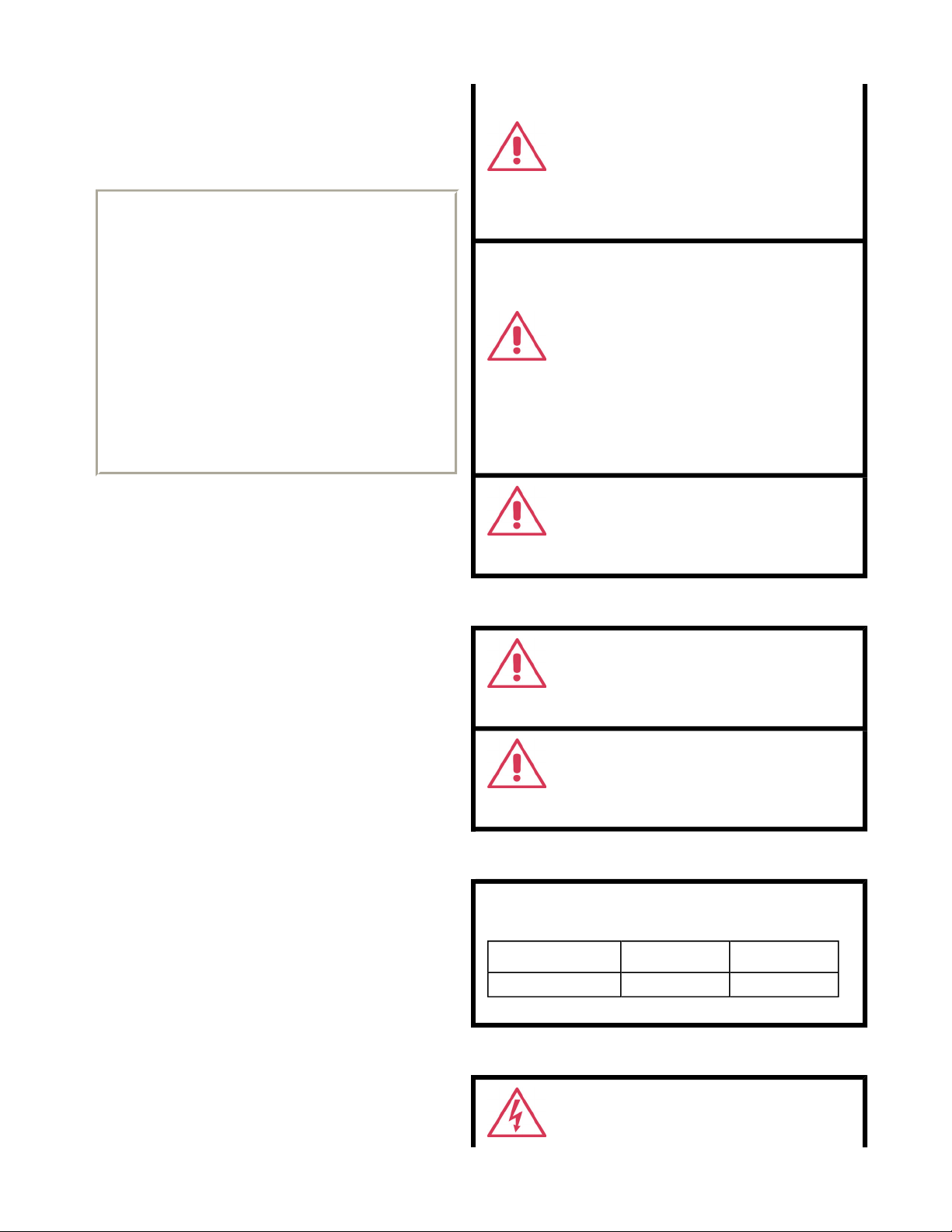
Safety Symbols and Terms

Where the following symbols or terms appear on the instrument’s front or rear panels, or in this manual, they alert you to important safety
considerations.

This symbol is used where caution is required. Refer to the accompanying information or documents in order to protect
against personal injury or damage to the instrument.

This symbol warns of a potential risk of shock hazard.

This symbol is used to denote the measurement ground connection.

This symbol is used to denote a safety ground connection.

This symbol shows that the switch is a On/Standby switch. When it is pressed, the DSO’s state toggles between
Operating and Standby state. This switch is not a disconnect device. To completely remove power to the DSO, the
power cord must be unplugged from the AC outlet after the DSO is placed in Standby state.

This symbol is used to denote "Alternating Current."

The CAUTION sign indicates a potential hazard. It calls attention to a procedure, practice or condition which, if not

CAUTION

WARNING

CAT I

followed, could possibly cause damage to equipment. If a CAUTION is indicated, do not proceed until its conditions are
fully understood and met.

The WARNING sign indicates a potential hazard. It calls attention to a procedure, practice or condition which, if not
followed, could possibly cause bodily injury or death. If a WARNING is indicated, do not proceed until its conditions are
fully understood and met.

Installation (Overvoltage) Category rating per EN 61010-1 safety standard and is applicable for the oscilloscope front
panel measuring terminals. CAT I rated terminals must only be connected to source circuits in which measures are
taken to limit transient voltages to an appropriately low level.

Operating Environment

The instrument is intended for indoor use and should be operated
in a clean, dry environment with an ambient temperature within
the range of 5 °C to 40 °C.

Direct sunlight, radiators, and other heat sources should

Note:

be taken into account when assessing the ambient temperature.

The design of the instrument has been verified to conform to EN
61010-1 safety standard per the following limits:

WARNING

The DSO must not be operated in explosive, dusty, or wet/damp
atmospheres.

Installation (Overvoltage) Categories II (Mains Supply Connector)
& I (Measuring Terminals)

Pollution Degree 2

Protection Class I

Note:

Installation (Overvoltage) Category II refers to local distribution
level, which is applicable to equipment connected to the mains
supply (AC power source).

Installation (Overvoltage) Category I refers to signal level, which
is applicable to equipment measuring terminals that are
connected to source circuits in which measures are taken to
limit transient voltages to an appropriately low level.

Pollution Degree 2 refers to an operating environment where
normally only dry non-conductive pollution occurs. Occasionally
a temporary conductivity caused by condensation must be
expected.

Protection Class I refers to a grounded equipment, in which
protection against electric shock is achieved by Basic Insulation
and by means of a connection to the protective ground
conductor in the building wiring.

CAUTION

Protect the DSO’s display touch screen from excessive impacts
with foreign objects.

CAUTION

Do not exceed the maximum specified front panel terminal (CH1,
CH2, CH3, CH4, EXT) voltage levels. Refer to Specifications for
more details.

Cooling Requirements

The instrument relies on forced air cooling with internal fans and
ventilation openings. Care must be taken to avoid restricting the
airflow around the apertures (fan holes) at the sides, front, and
rear of the DSO. To ensure adequate ventilation it is required to
leave a 10 cm (4 inch) minimum gap around the sides, front, and
rear of the instrument.

AC Power Source

The instrument operates from a single-phase, 100 to 240 V

(+/-10%) AC power source at 50/60 Hz (+/-5%), or single-phase
100 to 120 V

No manual voltage selection is required; the instrument
automatically adapts to line voltage.

Depending on the accessories installed (front panel probes, PC
port plug-ins, external printer, etc.), the instrument can draw up to
200 VA (4-channel models) or 170 VA (2-channel models).

(+/-10%) AC power source at 400 Hz (+/-5%).

rms

rms

CAUTION

Do not connect or disconnect probes or lest leads while they are
connected to a voltage source.

CAUTION

Do not block the ventilation holes located on both sides and rear
of the DSO.

CAUTION

Do not allow any foreign matter to enter the DSO through the
ventilation holes, etc.

Note:

The instrument automatically adapts itself to the AC line input
within the following ranges:

Voltage Range:

Frequency Range:

90 to 264 V

47 to 63 Hz 380 to 420 Hz

rms

90 to 132 V

rms

Power and Ground Connections

The instrument is provided with a grounded cord set containing a
molded three-terminal polarized plug and a standard IEC320
(Type C13) connector for making line voltage and safety ground
connection. The AC inlet ground terminal is connected directly to

WARNING

A

the frame of the instrument. For adequate protection against
electrical shock hazard, the power cord plug must be inserted into
a mating AC outlet containing a safety ground contact. Use only
the power cord specified for this instrument and certified for the
country of use.

The DSO should be positioned to allow easy access to the
socket-outlet. To completely remove power to the DSO, unplug
the instrument’s power cord from the AC outlet after the DSO is
placed in Standby state.

In Standby state the DSO is still connected to the AC supply. The
instrument can only be placed in a complete Power Off state by
physically disconnecting the power cord from the AC supply. It is
recommended that the power cord be unplugged from the AC
outlet if the DSO is not being used for an extended period of time.

See On/Standby Switch

for more information.

Electrical Shock Hazard!

Any interruption of the protective conductor inside or outside of
the DSO, or disconnection of the safety ground terminal creates a
hazardous situation.

Intentional interruption is prohibited.

CAUTION

The outer shells of the front panel terminals (CH1, CH2, CH3,
CH4, EXT) are connected to the instrument’s chassis and
therefore to the safety ground.

On/Standby Switch

The front panel On/Standby switch controls the operational state of the DSO. This toggle switch is activated by momentarily pressing and
releasing it.

There are two basic DSO states: On or Standby. In the "On" state, the DSO, including its computer subsystems (CPU, hard drive, etc,) is fully
powered and operational. In the "Standby" state, the DSO, including computer subsystems, is powered off with the exception of some
"housekeeping" circuitry (approximately 2 watts dissipation).

lways use the On/Standby switch to place the DSO in Standby state so that it executes a proper shutdown process (including a Windows

shutdown) to preserve settings before powering itself off. This can be accomplished by pressing and holding in the On/Standby switch for
approximately 5 seconds.

To power off completely, place the DSO in Standby state, then disconnect the power cord.

Note:

Calibration

The recommended calibration interval is one year. Calibration should be performed by qualified personnel only.

Cleaning

Clean only the exterior of the instrument, using a damp, soft cloth.
Do not use chemicals or abrasive elements. Under no
circumstances allow moisture to penetrate the instrument. To
avoid electrical shock, unplug the power cord from the AC outlet
before cleaning.

Electrical Shock Hazard!

No operator serviceable parts inside. Do not remove covers.

Refer servicing to qualified personnel.

WARNING

Abnormal Conditions

Operate the instrument only as intended by the manufacturer.

If you suspect the DSO’s protection has been impaired,
disconnect the power cord and secure the instrument against any
unintended operation.

The DSO’s protection is likely to be impaired if, for example, the
instrument shows visible damage or has been subjected to severe
transport stresses.

Proper use of the instrument depends on careful reading of all
instructions and labels.

Top of Page

Any use of the DSO in a manner not specified by the
manufacturer may impair the instrument’s safety protection. The
instrument and related accessories should not be directly
connected to human subjects or used for patient monitoring.

WARNING

FRONT PANEL CONTROLS

Front Panel Buttons and Knobs

The control buttons of the instrument's front panel are logically grouped into analog and special functional areas. Analog functions are included
in the Horizontal , Trigger , and Vertical groups of control buttons and knobs.

Some of the front panel knobs are also special function push buttons. By pressing the knobs, you can activate functions such as Find

Note:

Level, Zero Vertical Offset, and Zero Delay. The

Sometimes you may want to change a value without using the numeric keypad. In that case, simply touch once inside the data entry field in
the scope dialog area (the field will be highlighted in yellow), then use the Adjust

knob functions as a toggle between fine and coarse adjustment.

DJUST

A

knob to dial in values into the selected field.

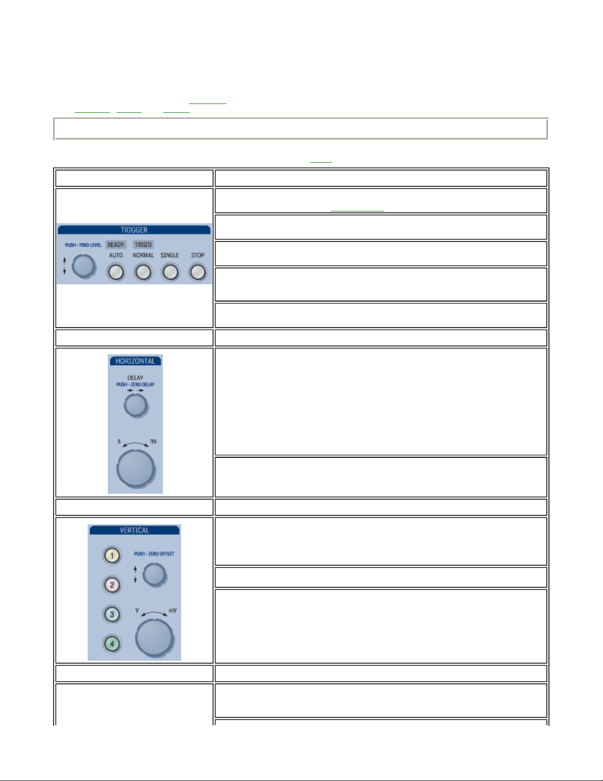
Trigger Control:

Horizontal Control:

The
which is indicated in the

Press

knob selects the trigger threshold level. Push this knob to quickly find the level,

EVEL

L

to display your trace.

UTO

A

Trigger

descriptor label

triggers the scope after a time-out, even if the trigger

UTO

A

.

conditions are not met.

N

triggers the scope each time a signal is present that meets the conditions set for the

ORMAL

type of trigger selected.

arms the scope to trigger once (single-shot acquisition) when the input signal meets

INGLE

S

the trigger conditions set for the type of trigger selected. If the scope is already armed, it will
force a trigger.

prevents the scope from triggering on a signal. If you boot up the instrument with the

TOP

S

trigger in Stop mode, the message "no trace available" will be displayed.

horizontally positions the scope trace on the display so you can observe the signal

DELAY

prior to the trigger time. It adjusts the pre- and post-trigger time. Push this knob to quickly set
the delay to zero, in which case the trigger point is positioned in the middle of the display grid.

When Zoom is selected, this button is used to position the zoom trace horizontally on the grid.

Vertical Control:

Cursor Control:

Sets the time/division of the timebase (acquisition system).

The

ERTICAL OFFSET

V

knob adjusts the vertical offset of a channel. Press the knobs to quickly

set the offset to zero for the selected channel.

When Zoom is selected, this button is used to position the zoom trace vertically on the grid.

The

OLTS/DIVISION

V

knob sets the vertical gain of the channel selected.

The channel number buttons only turn a channel on or off; they do not display the setup dialog
for the channel. A lighted channel button indicates that the channel trace is On and that the
front panel controls are dedicated to that channel.

To display a channel's setup dialog, select the channel from the

drop-down menu. Or,

Vertical

touch the channel descriptor label twice.

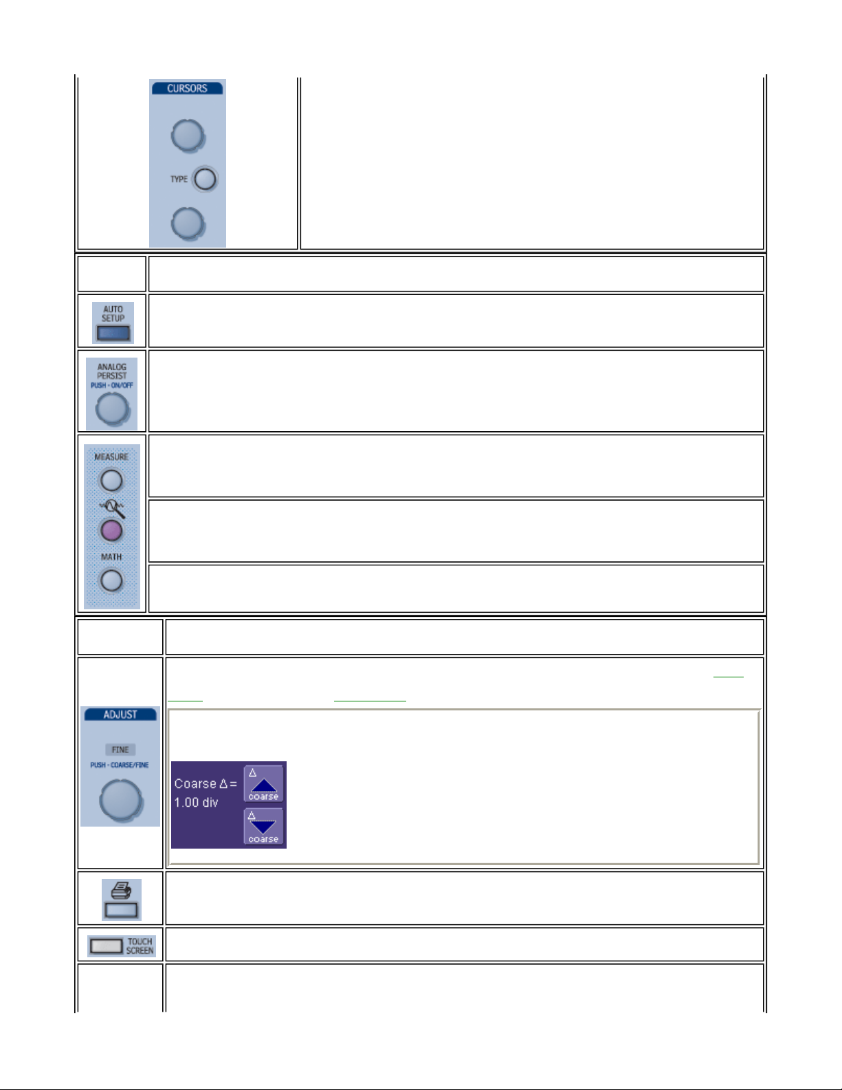
The

cursor button turns on cursors and, with each additional push, cycles through the

YPE

T

different types -- horizontal (time) and vertical (amplitude), then turns them off. For an FFT
math function, frequency cursors can also be displayed.

The top and bottom knobs control the vertical and horizontal position of the cursors,
depending on the type selected (vertical or horizontal). Cursors can be turned on by rotating
either knob, and the cursors' position can be read in the Cursors Setup dialog (selectable from
the menu bar) where you can also set both cursors to move in unison (tracking).

Push in the cursor control knobs at any time to return the cursors to their default starting
positions.

Cursor values are displayed on-screen in the channel/trace descriptor labels and underneath
the trigger and timebase descriptor labels.

Special
Features:

General
Control:

UTO SETUP

A

trigger conditions, to display a wide variety of signals.

NALOG PERSIST

A

automatically sets the scope's horizontal timebase (acquisition system), vertical gain and offset, as well as

provides a three dimensional view of the signal: time, voltage, and a third dimension related to the
frequency of occurrence, as shown by a color-graded (thermal) or intensity-graded (analog) display. Push the button to turn
persistence on, then continue pushing the button to cycle through analog and color-graded persistence, and finally to turn
persistence off. When color-graded persistence is selected, you can rotate the knob to vary the saturation level.

Pushing the

M

button opens the Measure dialog, which enables you to set up six parameter measurements with

EASURE

statistics. Push again to close the measure dialog.

The

UICKZOOM

Q

button toggles zooms of all displayed channel traces on and off. If there is a math trace displayed when you

push this button, the math trace will be automatically turned off to free a slot for a zoom trace.

Pushing the

button opens the Math setup dialog and turns on the math trace. Push again to close the Math dialog.

ATH

M

By default, the
knob to toggle to

by touching twice inside a data entry field . Then use the keypad to type in the value.

keypad

You can set the granularity (delta) of the coarse adjustment by double-tapping inside the data entry field, then

Note:

touching the

Advanced

knob makes coarse adjustments (that is, digits to the left of the decimal point). Press the Adjust

DJUST

A

and adjust digits to the right of the decimal point. To enter exact values, you can also display a

Fine

checkbox in the pop-up numeric keypad. The keypad presents

delta up/down buttons to

Coarse

set the delta:

.

In the pop-up keypad, be sure to leave the

checkbox unchecked to adjust the coarse delta.

Fine

The printer button prints the displayed screen to a file, a printer, the clipboard, or sends it as e-mail. Select the device and
format it in the Utilities - Hardcopy dialog.

T

C

OUCH SCREEN

LEAR SWEEPS

activates or deactivates the touch screen.

clears data from multiple sweeps (acquisitions) including: persistence trace displays, averaged traces,

and parameter statistics.

Top of Page

ON-SCREEN TOOLBARS, ICONS, AND DIALOG BOXES

Menu Bar Buttons

The menu bar buttons at the top of the scope's display are designed for quick setup of common functions. At the right end of the menu bar is a
quick setup button that, when touched, opens the setup dialog associated with the trace or parameter named beside it. The named trace or

parameter is the one whose setup dialog you last opened: . This button also appears as an undo button after front

panel buttons
after you perform the Autosetup or QuickZoom operation.

UTOSETUP

A

and

UICKZOOM

Q

are pressed. If you want to perform an Undo operation, it must be the very next operation

Dialog Boxes

The dialog area occupies the bottom one-third of the screen. To expand the signal display area, you can minimize each dialog box by touching
the

Top of Page

tab at the right of the dialog box.

Close

ALTERNATE ACCESS METHODS

The instrument often gives you more than one way to access dialogs and menus.

Mouse and Keyboard Operation

In the procedures we focus on front panel and touch-screen operation, but if you have a mouse connected to the instrument, you can also
click on objects. Likewise, if you have a keyboard connected, you can use it instead of the virtual keyboard provided by the instrument.

Tool Bar Buttons

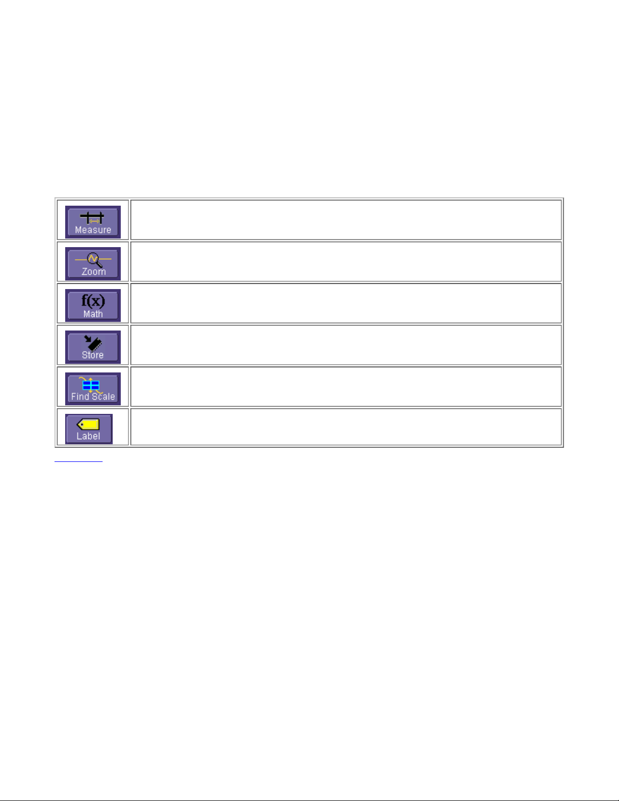
The procedures also focus on the use of the menu bar at the top of the screen to access dialogs and menus. However, on several dialogs
common functions are accessible from a row of buttons that save you a step or two in accessing their dialogs. For example, at the bottom of
the Channel Setup dialog, these buttons perform the following functions:

A pop-up menu allows you to select up to six measurements to compute on this channel without leaving the
Channel Setup dialog. The parameter automatically appears below the grid.

Creates a zoom trace of the channel trace whose dialog is currently displayed.

A pop-up menu allows you to select a math function from this menu without leaving the Channel Setup dialog. A
math trace of the channel whose dialog is currently open is automatically displayed.

Loads the channel trace into the next available memory location (M1 to M4).

Top of Page

Automatically performs a vertical scaling that fits the waveform into the grid.

Opens a Labeling pop-up menu that allows you to create labels tied to the waveform.

TRACE DESCRIPTORS

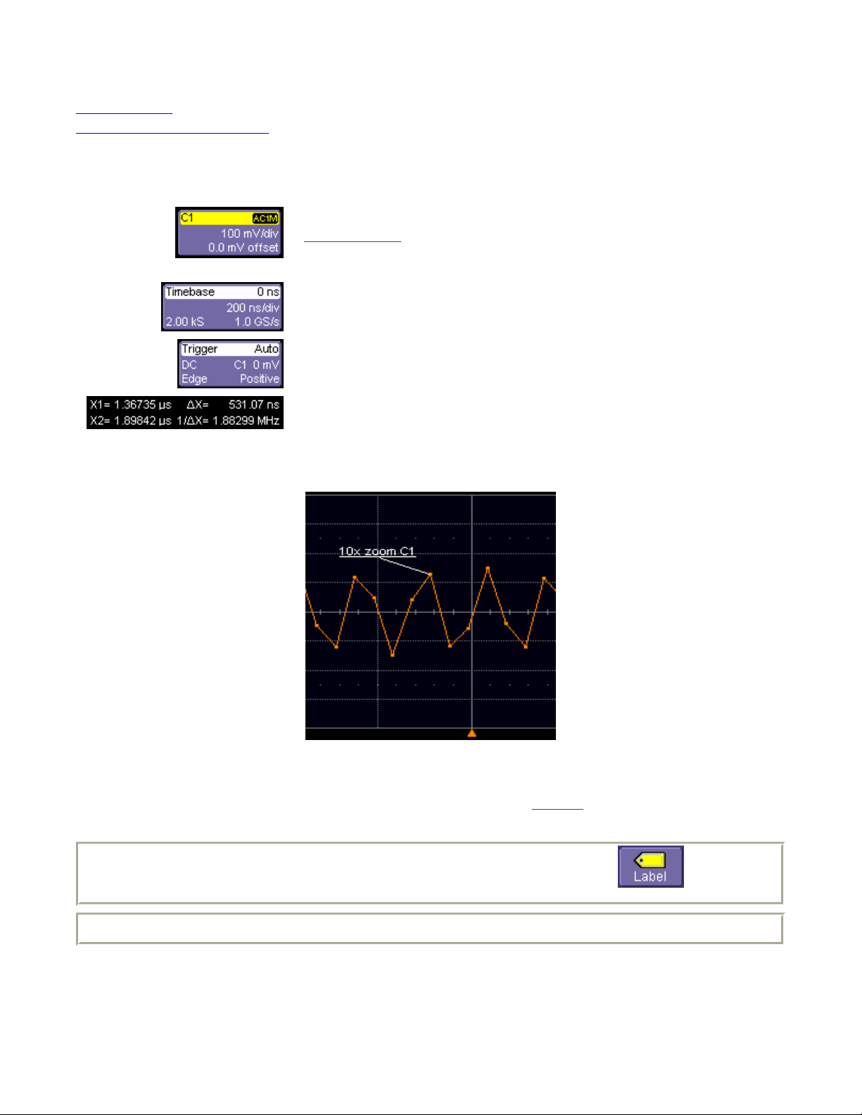
V

Trace Annotation

To Turn On a Channel Trace Label

Vertical and horizontal trace descriptors (labels) are displayed below the grid. They provide a summary of your channel, timebase, and trigger
settings. To make adjustments to these settings, touch the respective label to display the setup dialog for that function. Channel labels need to
be touched twice unless they are active.

Channel trace labels show the vertical settings for the trace, as well as cursor information if
cursors are in use. In the title bar of the label are also included indicators for deskew (DSQ),
coupling (DC/GND), bandwidth limiting (BWL), and averaging (AVG). These indicators have a

long and short form

Besides channel traces, math and parameter measurement labels are also displayed. Labels
are displayed only for traces that are turned on.

.

The title bar of the
sampling information is given below the title bar.

The title bar of the
title bar is given the coupling (DC), trigger type (Edge), source (C1), level (0 mV), and slope
(Positive).

Shown below the TimeBase and Trigger labels is setup information for horizontal cursors,
including the time between cursors and the frequency.

TimeBase

Trigger

label shows the trigger delay setting. Time per division and

label shows the trigger mode: Auto, Normal, or Stopped. Below the

Trace Annotation

The instrument gives you the ability to add an identifying label, bearing your own text, to a waveform display:

For each waveform, you can create multiple labels and turn them all on or all off. Also, you can position them on the waveform by dragging or
by specifying an exact horizontal position.

To Annotate a Waveform

1. Touch the waveform you want to annotate, then
you are creating a label for the first time for this waveform,
under

If the dialog for the trace you want to annotate is currently displayed, you can touch the label button at the bottom to

Note 1:

display the Trace Annotation setup dialog.

You may place a label anywhere you want on the waveform. Labels are numbered sequentially according to the order in which they

Note 2:

are added, and not according to their placement on the waveform.

2. If you want to change the label's text, touch inside the

3. To place the label precisely, touch inside the

4. To add another label, touch the

5. To make the labels visible, touch the

on the keyboard when you are done. Your edited text will automatically appear in the label on the waveform.

O.K.

touch the label you want to change.

Labels

Add label

iew labels

Set label...

Horizontal Pos.

button. To delete a label, select the label from the list, then touch the

checkbox.

in the pop-up menu. A dialog box

is displayed with default text. If you are modifying an existing label,

Label1

Label Text

field. A pop-up keyboard appears for you to enter your text. Touch

field and enter a horizontal value, using the pop-up numeric keypad.

opens in which to create the label. If

Remove label

button.

To Turn On a Trace

z

On the front panel, press a channel select button, such as , to display the trace label for that input channel and turn on the
channel. Touch the channel trace label to open the dialog box.

z To turn on a math function trace, press the

front panel button or touch

ATH

M

in the menu bar, then

Math

Math Setup...

in the drop-

down menu. Touch the On checkbox for the trace you want to activate.

z You can also quickly create traces (and turn on the trace label) for math functions and memory traces, without leaving the Vertical

Adjust dialog, by touching the icons at the bottom of the Vertical Adjust dialog: , , ,

.

Whenever you turn on a channel, math, or memory trace via the menu bar, the dialog at the bottom of the screen automatically switches to the
vertical setup or math setup dialog for that selection. You can configure your traces from here, including math setups.

The channel number appears in the tab of the "Vertical Adjust" dialog, signifying that all controls and data entry fields are dedicated to the
selected trace.

Top of Page

SCREEN LAYOUT

The instrument's screen is divided into three areas:

z menu bar

z signal display area

z dialog area

Menu Bar

The top of the screen contains a toolbar of commonly used functions. Whenever you touch one of these buttons, the dialog area at the bottom
of the screen switches to show the setup for that function.

Signal Display Grid

You can set up the signal display area by touching in the toolbar, then the tab. The display dialog offers a choice
of grid combinations and a means to set the grid intensity.

Dialog Area

The lower portion is where you make selections and input data. The dialog area is controlled by both toolbar touch buttons and front panel
push buttons.

Top of Page

HARDWARE INSTALLATION

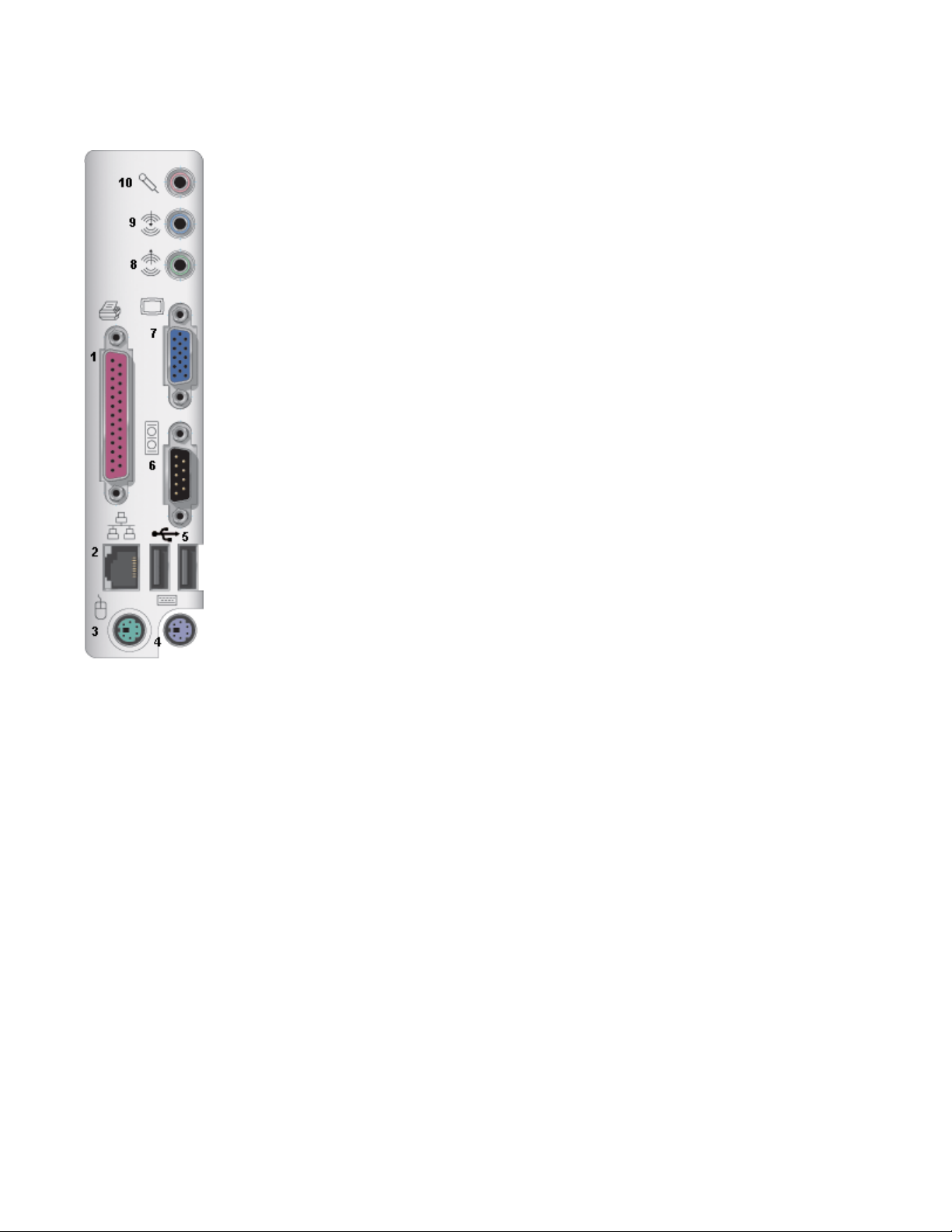
Instrument I/O Panel

(1) Centronics Port; (2) Ethernet Port; (3) Mouse; (4) Keyboard; (5) USB Ports; (6) RS-232-C Port; (7) External VGA Monitor; (8) Line
In; (9) Speakers; (10) Microphone

SOFTWARE

Checking the Scope Status

To find out the scope's software and hardware configuration, including software version and installed options, proceed as follows:

1. In the menu bar, touch .

2. Touch the tab.

You can find information related to hard drive memory, etc. as follows:

1. Minimize the instrument application by touching , then selecting

2. Touch the

Top of Page

taskbar button and, per usual Windows® operation, open Windows Explorer.

Start

Minimize

in the drop-down menu.

DEFAULT SETTINGS

WaveMaster and WavePro 7000 Series DSOs

You can reset the scope to default settings by simply pressing the
Channel1 and Channel 2, with no processing enabled.

Other default settings are as follows:

Vertical Timebase Trigger

50 mV/div 50.0 ns/div DC50Ω (WaveMaster, DDA, SDA), AC1MΩ (WavePro), C1, 0 mV level

EFAULT SETUP

D

push button on the front panel. This feature turns on

0 V offset 10.0 GS/s

0 s delay Auto trigger mode

edge trigger
positive edge

DDA, SDA, and WaveRunner DSOs

On your front panel, the

1. Press the

You can also touch

Note:

2. Touch the "Recall Setup" tab in the dialog.

3. Then touch the on-screen

Top of Page

EFAULT SETUP

D

AVE/RECALL

S

in the menu bar, then

File

push button does not exist. For these instruments, therefore, to recall a default setup

push button to the left of the

Recall Default Setup

RIVE ANALYSIS

D

Recall Setup...

button

.

push button.

in the drop-down menu.

ADDING A NEW OPTION

To add a software option you need a key code to enable the option. Call your local salesman or LeCroy Customer Support to place an order
and receive the code.

To add the software option do the following:

1. In the menu bar, touch .

2. In the dialog area, touch the tab.

3. Touch .

4. Use the pop-up keyboard to type the key code. Touch

5. The name of the feature you just installed is shown below the list of key codes. You can use the scroll buttons to see the name of the
option installed with each key code listed:

on the keyboard to enter the information.

O.K.

Top of Page

RESTORING SOFTWARE

Restarting the Application

Upon initial power-up, the scope will load the instrument application software automatically. If you exit the application and want to reload it,

touch the shortcut icon on the desktop: .

If you minimize the application, touch the appropriate task bar or desktop button to maximize it:

.

Restarting the Operating System

If you need to restart the Windows® operating system, you will have to reboot the scope by pressing and holding in the power switch for 10
seconds, then turning the power back on.

Top of Page

PROBUS INTERFACE

LeCroy's ProBus® probe system provides a complete measurement solution from probe tip to oscilloscope display. ProBus allows you to
control transparent gain and offset directly from your front panel. It is particularly useful for voltage, differential, and current active probes. It
uploads gain and offset correction factors from the ProBus EPROMs and automatically compensates to achieve fully calibrated
measurements.

This intelligent interconnection between your instrument and a wide range of accessories offers important advantages over standard BNC and
probe ring connections. ProBus ensures correct input coupling by auto-sensing the probe type, thereby eliminating the guesswork and errors
that occur when attenuation or amplification factors are set manually.

Top of Page

AUXILIARY OUTPUT SIGNALS

In addition to a standard 1 V, 1 kHz calibration signal on the front panel, the following signals can be output through the AUX OUTPUT
connector at the rear of the scope:

Trigger Out -- can be used to trigger another scope.

Trigger Enabled -- can be used as a gating function to trigger another instrument when the scope is ready.

Pass/Fail -- allows you to set a pulse duration from 1 ms to 500 ms; generates a pulse when pass/fail testing is active and
conditions are met.

Aux Output Off -- turns off the auxiliary output signal.

To Set Up Auxiliary Output

1. In the menu bar, touch

2. Touch the

3. Touch one of the buttons under

Top of Page

Aux Output

Utilities

tab.

, then

Utilities Setup...

Use Auxiliary Output For

in the drop-down menu.

.

SAMPLING MODES

Depending on your timebase, you can choose either Single-shot (Real Time) , RIS , or Roll mode sampling.

To Select a Sampling Mode

1. In the menu bar, touch

2. In the "Horizontal" dialog, touch a

Top of Page

Timebase

, then

Horizontal Setup...

Sample Mode

in the drop-down menu.

button.

SINGLE-SHOT SAMPLING MODE

A

To Select a Sampling Mode

Basic Capture Technique

single-shot acquisition is a series of digitized voltage values sampled on the input signal at a uniform rate. It is also a series of measured
data values associated with a single trigger event. The acquisition is typically stopped a defined number of samples after this event occurs: a
number determined by the selected trigger delay and measured by the timebase. The waveform's horizontal position (and waveform display in
general) is determined using the trigger event as the definition of time zero.

You can choose either a pre- or post-trigger delay. Pre-trigger delay is the time from the left-hand edge of the display grid forward to the
trigger event, while post-trigger delay is the time back to the event. You can sample the waveform in a range starting well before the trigger
event up to the moment the event occurs. This is 100% pre-trigger, and it allows you to see the waveform leading up to the point at which the
trigger condition was met and the trigger occurred. (The instrument offers up to the maximum record length of points of pre-trigger
information.) Post-trigger delay, on the other hand, allows you to sample the waveform starting at the equivalent of 10,000 divisions after the
event occurred.

Because each instrument input channel has a dedicated ADC (Analog-to-Digital Converter), the voltage on each is sampled and measured at
the same instant. This allows very reliable time measurements between the channels.

On fast timebase settings, the maximum single-shot sampling rate is used. But for slower timebases, the sampling rate is decreased and the
number of data samples maintained.

The relationship between sample rate, memory, and time can be simply defined as:

and

Top of Page

RIS SAMPLING MODE -- FOR HIGHER SAMPLE RATES

To Select a Sampling Mode

RIS (Random Interleaved Sampling) is an acquisition technique that allows effective sampling rates higher than the maximum single-shot
sampling rate. It is used on repetitive waveforms with a stable trigger. The maximum effective sampling rate of 50 GS/s can be achieved with
RIS by making 100 single-shot acquisitions at 500 MS/s. The bins thus acquired are positioned approximately 20 ps apart. The process of
acquiring these bins and satisfying the time constraint is a random one. The relative time between ADC sampling instants and the event
trigger provides the necessary variation, measured by the timebase to 5 ps resolution.

The instrument requires multiple triggers to complete an acquisition. The number depends on the sample rate: the higher the sample rate, the
more triggers are required. It then interleaves these segments (see figure
the maximum single-shot sampling rate. However, the real-time interval over which the instrument collects the waveform data is much longer,
and depends on the trigger rate and the amount of interleaving required. The oscilloscope is capable of acquiring approximately 40,000 RIS
segments per second.

) to provide a waveform covering a time interval that is a multiple of

Top of Page

ROLL MODE

To Select a Sampling Mode

Roll mode can be selected when the timebase mode is real time, time per division is > 200 ms/div, and the sampling rate is < 200 kS/s.

Roll mode is selected automatically when the above criteria are met. Otherwise, the scope is in real-time mode.

Roll mode displays, in real time, incoming points in single-shot acquisitions that have a sufficiently low data rate. The oscilloscope rolls the
incoming data continuously across the screen until a trigger event is detected and the acquisition is complete. The parameters or math
functions connected to each channel are updated every time the roll mode buffer is updated, as if new data is available. This resets statistics
on every step of Roll mode that is valid because of new data.

If the processing time is greater than the acquire time, the data in memory gets overwritten. In this case, the instrument issues the

Note:

warning:

Top of Page

Channel data is not continuous in ROLL mode!!!

and rolling will start over again.

ADJUSTING SENSITIVITY AND POSITION

To Adjust Sensitivity

1. Press the appropriate channel push button, for example to select channel 1. Or touch the channel descriptor label.

2. Turn the volts per division knob
type in a value using the pop-up keypad, or use the up/down arrows.

3. The voltage that you set is displayed in the trace descriptor label

for the selected channel. Or you can touch inside the Volts/Div field in the channel setup dialog and

and in the

Volts/Div

field.

To Adjust the Waveform's Position

Turn the vertical offset adjust knob. Or you can touch inside the
offset to zero press the front panel Offset button, or touch the Zero Offset button directly below the Offset field in the channel setup dialog.

Top of Page

field and type in a value on the pop-up keypad. To set the vertical

Offset

COUPLING

The choices of coupling are as follows:

z DC 50 Ω

z GROUND

z DC 1 MΩ

z AC 1 MΩ

The choices offered may differ if a ProBus® probe is connected to the instrument.

Note:

Overload Protection

The maximum input voltage is 4 V peak. Whenever the voltage exceeds this limit, the coupling mode automatically switches from DC 50 Ω to
GROUND. You will then have to manually reset the coupling to DC 50 Ω, as described next.

To Set Coupling

1. In the menu bar, touch the
label twice.

2. Touch inside the

Top of Page

Coupling

button, then

Vertical

field and select a coupling mode from the pop-up menu.

Channel X Setup...

in the drop-down menu. Or you can touch the channel descriptor

PROBE ATTENUATION

To Set Probe Attenuation

LeCroy's ProBus® system automatically senses probes and sets their attenuation for you. If you want to set the attenuation manually,

1. In the menu bar, touch

2. Touch inside the
value using the pop-up numeric keypad.

Top of Page

Probe Atten.

, then select a channel from the drop-down menu.

Vertical

data entry field

. Touch a divide-by menu selection or touch

(variable). If you choose

Var

Var

, type in a

BANDWIDTH LIMIT

Reducing the bandwidth also reduces the signal and system noise, and prevents high frequency aliasing.

To Set Bandwidth Limiting

To set bandwidth limiting

1. In the menu bar, touch

2. Touch inside the

z

Full

z 200 MHz (not available on 200 MHz bandwidth models)

z

20 MHz

Top of Page

Bandwidth

, then select a channel from the drop-down menu. Or you can touch the channel descriptor label twice.

Vertical

field and select a bandwidth limit value from the pop-up menu. The options are

QUICKZOOM

QuickZoom automatically displays a zoom of the channel or trace on a new grid.

To Turn On a Zoom

Touch the

button in the channel dialog.

Zoom

FINDING SCALE

You can access the
an appropriate Volts/Div scale to fully display the waveform.

Find Scale

button from the channel setup dialog. This feature automatically calculates peak-to-peak voltage, and chooses

To Use Find Scale

1. Touch the trace label for the waveform you desire.

2. Touch the

Find Scale

icon.

VARIABLE GAIN

Variable Gain lets you change the granularity with which the gain is incremented. For example, when
increase or decrease in preset increments of 10 or 100 mV each time you touch the

However, when
the waveform.

Variable Gain

is enabled, you can increase or decrease the gain in increments as small as 1 mV, depending on the scale of

Up/Down

buttons.

To Enable Variable Gain

1. Touch the descriptor label for the waveform whose gain you want to vary.

2. Touch the

Variable Gain

check box.

Variable Gain

is disabled, the gain will

CHANNEL DESKEW

Unlike the Deskew math function, channel Deskew does no resampling, but instead adjusts the horizontal offset by the amount that you enter.
The valid range is dependent on the current timebase +/- 9 divisions.

To Set Up Channel Deskew

1. In the menu bar, touch

2. Touch inside the

Deskew

; from the drop-down menu, select a channel to set up.

Vertical

data entry field and enter a value using the pop-up numeric keypad.

TIMEBASE SETUP AND CONTROL

Set up the timebase by using the front panel

For additional timebase setups

1. Touch

2. Touch inside the

3. Touch inside the

Timebase

adjust the value.

to zero.

in the menu bar, then

Time/Division

data entry field and type in a value, using the pop-up keypad. Touch the

Delay

Horizontal

Horizontal Setup...

data entry field and enter a value using the pop-up numeric keypad, or use the up/down arrows to

controls, just as for analog scopes.

in the drop-down menu. The "Horizontal" dialog appears.

Set To Zero

button to set the delay

DUAL CHANNEL ACQUISITION

Combining of Channels

During 4-channel operation, channels 1 and 2 or channels 3 and 4 are automatically combined to increase sample rate, memory, or both in
order to capture and view a signal in all its detail. To maximize sampling rate when using only two channels, choose either channel 1 or 2 and
either channel 3 or 4. When channels are combined, uncombined channels like EXT BNC remain available for triggering, even though they are
not displayed.

Top of Page

AUTOSETUP

When channels are turned on, Autosetup operates only on those turned-on channels. If no channels are turned on, all channels are affected.
When more than one channel is turned on, the first channel in numerical order with a signal applied to it is automatically set up for edge
triggering.

You can perform an autosetup of all these functions together by simply pressing on the front panel, or by touching

in the Vertical, Timebase, or Trigger drop-down menu.

Top of Page

Autosetup

SIMPLE TRIGGERS

A

A

To Set Up an Edge Trigger

To Set Up a SMART Trigger

Trigger Setup Considerations

Edge Trigger on Simple Signals

The instrument uses many waveform capture techniques that trigger on features and conditions that you define. These triggers fall into two
major categories:

z

z

Use Edge Triggers for simple signals, and the SMART Triggers for signals with rare features, like glitches.

– activated by basic waveform features or conditions such as a positive or negative slope, and hold-off

Edge

SMART Trigger®

– sophisticated triggers that enable you to use basic or complex conditions for triggering.

Control Edge Triggering

Horizontal:

in the timebase setup dialog and enter a value, using the pop-up keypad.

The trigger location is shown by a marker below the grid .

Post-trigger delay is indicated by a left-pointing arrow below-left of the grid . The time value is given in the title line of the

label below-right of the grid.

Vertical:

Turn this knob to adjust the level of the trigger source or the highlighted trace. Level defines the source voltage at which the trigger will
generate an event — a change in the input signal that satisfies the trigger conditions.

lternatively, in the "Trigger" dialog, you can touch inside the

a level of zero volts, touch the

n arrow on the left side of the grid shows the threshold position. This arrow is only visible if the trigger source is displayed.

Turn the

Turn the

L

knob in the HORIZONTAL control group to adjust the trigger's horizontal position. Or, touch inside the

DELAY

knob in the TRIGGER control group to adjust the trigger's vertical threshold.

EVEL

field and type in a value, using the pop-up numeric keypad. To quickly set

Zero Level

button directly below the

Level

Coupling

field.

Delay

TimeBase

field

To Set Up an Edge Trigger

Channel Setup

1. In the menu bar, touch

2. Touch the

3. Touch inside the

4. Touch inside the
increase or decrease the value in increments of 1 mV. Or, touch one of the preset value buttons

Max.

Default

Min.

5. Select the holdoff by touching the
specify the unit of time
the preset value buttons .

The preset

Max.

trigger button under the

Edge

Trigger On

Level

1.000 V

0 mV

–1.000 V

, or use the up/down buttons to increase or decrease the time value in increments of 200 ps. Or, touch one of

values are as follows:

Time

20.0 s

, then select

Trigger

data entry field and select an input from the pop-up menu

data entry field

Time

Trigger Setup...

Trigger

. In the pop-up numeric keypad , enter a value in millivolts or use the up/down buttons to

or

buttons , . Using the pop-up numeric keypad, enter a value and

Events

from the drop-down menu.

tab.

.

.

Default

50.0 ns

The preset

Default

6. Choose

Top of Page

Min.

Max.

Min.

2 ns

values are as follows:

Events

1,000,000,000 events

Positive

or

Negative

1 event

1 event

slope

.

SMART TRIGGERS

Glitch Trigger

Width Trigger

Interval Trigger

State Trigger

Qualified Trigger

Dropout Trigger

ogic Trigger

L

Runt Trigger

Slew Rate Trigger

TV Trigger

o Set Up Edge Trigger

T

Trigger Setup Considerations

Width Trigger

To Set Up Width Trigger

How Width Trigger Works

Width trigger allows you to define a positive- or negative-going pulse width bounded by a voltage level, above or below which a trigger will
occur. You can specify a pulse width and voltage range, within or outside of which a trigger will occur.

To Set Up Width Trigger

1. In the menu bar, touch

2. Touch the

Smart Trigger

Trigger

button.

, then

Trigger Setup...

in the drop-down menu.

3. Touch inside the

4. Touch inside the

5. Touch inside the

6. Select positive or negative slope.

7. Touch the

Or touch the

Or touch the

Touch the
and

Alternatively, touch the
data entry fields and enter values using the pop-up keypads.

Or touch the

LessThan

GreaterThan

InRange

Delta

data entry fields and enter values using the pop-up numeric keypads.

Delta

OutOfRange

field and select

Type

Trigger On

Level

button to set up a nominal range, plus or minus a delta value in seconds. Touch inside the

data entry field and select a source

data entry field and enter a value using the pop-up numeric keypad.

button and enter a pulse-width value in the

button and enter a pulse-width value in the

button.

Limits

button and perform the same range setups as for InRange triggering.

Width

button to set up a precise pulse-width range. Touch inside the

Glitch Trigger

To Set Up Glitch Trigger

How Glitch Trigger Works

trigger .

on which to trigger.

Upper Limit

data entry field.

Lower Limit

data entry field.

Lower Limit

Nominal Width

and

Upper Limit

Glitch trigger can be used to catch glitches. You can specify a pulse width or a pulse width range.

Pulse smaller than selected pulse width:

negative) when the pulse width is less than or equal to the set width.

The timing for the width is initialized and restarted on the opposite slope to that selected. You can set widths from 600 ps to 20 s.

If the glitch's width is narrower than the signal's width, set the trigger to a narrower width than that of the signal. The signal's width, as

NOTE:

determined by the instrument trigger comparator, depends on the DC trigger level. If that level were to be set at the middle of a sine wave,
for example, the width could then be considered as the half period. But if the level were higher, the signal's width would be considered to be
less than the half period.

Set a maximum pulse width. This glitch trigger is generated on the selected edge (positive or

Glitch Trigger: In this example triggering on a pulse width less than or equal to the width selected. The broken upward-pointing
arrow indicates a potential trigger, while the bold one shows where the actual trigger occurs.

To Set Up Glitch Trigger

1. In the menu bar, touch

2. Touch the

3. Touch inside the

4. Touch inside the

5. Touch inside the

6. Select positive or negative slope.

7. Define the width of the glitch you are looking for. You can trigger on any glitch less than a chosen pulse-width (
can trigger on a chosen range (

InRange

8. Touch inside the limit field or fields and enter a time value using the pop-up numeric keypad.

Smart Trigger

Type

Trigger On

Level

button; the

field and select

Upper Limit

, then

Trigger

button.

data entry field and enter a value using the pop-up numeric keypad.

Trigger Setup...

trigger .

Glitch

data entry field and select a source

and

Lower Limit

). Touch the

InRange

in the drop-down menu.

on which to trigger.

LessThan

fields are displayed.

button; the

Upper Limit

data entry field alone is displayed. Touch the

Upper Limit

); or you

Interval Trigger (optional with WS-ADVTRIG package)

To Set Up Interval Trigger

How Interval Triggers Work

While Glitch trigger performs over the width of a pulse, Interval trigger performs over the width of an interval, with the signal duration (period)
separating two consecutive edges of the same polarity: positive to positive or negative to negative. Use Interval trigger to capture intervals that
fall short of, or exceed, a given time limit. In addition, you can define a width range to capture any interval that is itself inside or outside the
specified range: an exclusion trigger by interval.

Interval Less Than:

between two like edges of the same slope (positive, for example).

The trigger is generated on the second (positive) edge if it occurs within the set interval. The instrument initializes and restarts the timing for

For this Interval Trigger, generated on a time interval smaller than the one that you set, choose a maximum interval

the interval whenever the selected edge occurs. You can set an interval from 2 ns to 20 s.

p

Interval Trigger that triggers when the interval width is smaller than the selected interval. The broken, upward-pointing arrow
indicates a potential trigger, while the bold one shows where the actual trigger occurs — on the positive edge within the selected
interval.

Interval Greater Than:

two edges of the same slope. The instrument generates the trigger on the second edge if it occurs after the set interval. The timing for the
interval is initialized and restarted whenever the selected edge occurs. You can set an interval from 2 ns to 20 s.

For this Interval Trigger, generated on an interval larger than the one that you set, select a minimum interval between

Interval Trigger that triggers when the interval width is larger than the set interval. The broken upward-pointing arrow indicates a

otential trigger, while the bold one shows where the actual trigger occurs — on the positive edge after the selected interval.

Interval In Range:

The instrument initializes and restarts the timing for the interval whenever the selected edge occurs. You can set an interval from 2 ns to 20 s.

This Interval Trigger is generated whenever an interval between two edges of the same slope falls within a selected range.

Interval Trigger that triggers when the interval falls within the selected range:
t1 = range's lower time limit; t2 = range's upper limit. The broken upward-pointing arrow indicates a potential trigger, while the bold
one indicates where the actual trigger occurs — on the positive edge within the selected range.

To Set Up Interval Trigger

1. In the menu bar, touch

2. Touch the

Smart Trigger

Trigger

button.

, then

Trigger Setup...

in the drop-down menu.

3. Touch inside the

4. Touch inside the

5. Touch inside the

6. Select positive or negative slope.

7. Touch the

Or touch the

Or touch the

Or touch the

LessThan

GreaterThan

InRange

Touch the

and

Width

Touch the
enter values using the pop-up numeric keypads.

OutOfRange

field and select

Type

Trigger On

Level

Delta

Delta

Limits

data entry field and select a source

data entry field and enter a value using the pop-up numeric keypad.

button and enter a pulse-width value in the

button and enter a value in the

button.

button to set up a nominal range, plus or minus a delta value, in seconds. Touch inside the
data entry fields and enter values using the pop-up numeric keypads.

button to set up a precise range. Touch inside the

button and perform the same Delta or Limits setup as for InRange triggering.

Interval

trigger .

Lower Limit

on which to trigger.

Upper Limit

data entry field.

data entry field.

Lower Limit

and

Upper Limit

Nominal

data entry fields and

Qualified Trigger (optional with WS-ADVTRIG package)

To Set Up Qualified Triggers

How Qualified Triggers Work

Use a signals transition above or below a given level (its validation) as an enabling (qualifying) condition for a second signal that is the trigger
source. These are Qualified triggers. For Edge Qualified triggers (the default) the transition is sufficient and no additional requirement is placed
on the first signal. For State Qualified triggers the amplitude of the first signal must remain in the desired state until the trigger occurs. A
qualified trigger can occur immediately after the validation, or following a predetermined time delay or number of potential trigger events. The
time delay or trigger count is restarted with every validation.

Within Time

creates a time window within which a trigger can occur.

Wait Time

can occur. The timing for the delay is restarted when the selected pattern begins.

Events

conditions. On the selected event of the trigger source and while the pattern is present, a trigger can occur. The count is initialized and started
whenever the selected pattern begins, and continues while the pattern remains. When the selected count is reached, the trigger occurs.

Edge Qualified and Wait: Trigger after timeout. The broken upward-pointing arrows indicate potential triggers, while the bold ones
show where the actual triggers occur.

To Set Up an Edge Qualified Trigger

1. In the menu bar, touch

2. Touch the

determines a delay from the start of the desired pattern. After the delay (timeout) and while the pattern is present, a trigger

determines a minimum number of events of the trigger source. An event is generated when a trigger source meets its trigger

Smart Trigger

Trigger

button.

, then

Trigger Setup...

in the drop-down menu.

3. Touch inside the

4. Touch inside the

5. Select

6. Touch inside the

7. Touch inside the field below the

Positive

If you select an input channel or external source, touch inside the
Then touch inside the

If you want to set a holdoff in time or events, touch one of the

field and select

Type

Trigger On

or

Negative

After

data entry field and select a source

slope.

data entry field and select the qualifying signal source from the pop-up menu.

Qual Level

Qualify

field and set a voltage level using the pop-up numeric keypad.

Qualify by:

trigger .

on which to trigger.

has gone

Qualify by:

buttons and enter a value using the numeric keypad.

data entry field and select a logic level:

buttons: , ,

or

Above

.

Below

State Trigger

To Set Up a State Qualified Trigger

State trigger is another Qualified trigger; however, instead of using the edges of the qualifying inputs, State trigger uses the logic state of the
inputs to qualify the trigger. Therefore, the pattern must become true and remain true (for a period of time or number of events that you
specify) to qualify the trigger.

.

See also How Qualified Triggers Work.

State Qualified and Wait: Trigger after timeout. The broken upward-pointing arrows indicate potential triggers, while the bold arrows
show where the actual triggers occur.

To Set Up a State Qualified Trigger

1. In the menu bar, touch

2. Touch the

Smart Trigger

Trigger

, then

button.

Trigger Setup...

in the drop-down menu.

3. Touch inside the

4. Touch inside the

5. Select

6. Touch inside the

7. Touch inside the field below the holdoff buttons and set a value using the numeric keypad.

Positive

If you select an input channel or external source, touch inside the
Then touch inside the

If you want to set a holdoff in time or events, touch one of the holdoff buttons: , ,

field and select

Type

Trigger On

or

Negative

has gone

Qual Level

trigger .

State

data entry field and select a source

slope.

data entry field and select the qualifying signal source from the pop-up menu.

field and set a voltage level using the pop-up numeric keypad.

on which to trigger.

has gone

data entry field and select a logic level:

or

Above

.

Below

Dropout Trigger (optional with WS-ADVTRIG package)

To Set Up Dropout Trigger

Used primarily in single-shot applications, and usually with a pre-trigger delay, Dropout trigger can detect lost signals. The trigger is generated
at the end of the timeout period following the last trigger source transition. You can set a timeout period from 2 ns to 20 s.

How Dropout Trigger Works

.

A

Dropout Trigger: occurs when the timeout has expired. The bold upward-pointing arrows show where the trigger occurs.

To Set Up Dropout Trigger

1. In the menu bar, touch

2. Touch the

Smart Trigger

Trigger

button.

, then

Trigger Setup...

in the drop-down menu.

3. Touch inside the

4. Touch inside the Touch inside the

5. Select

6. Touch inside the

7. Touch inside the

Positive

field and select

Type

Trigger On

or

Negative

Level

Trigger after timeout

slope.

field and enter a voltage value.

Dropout

data entry field and enter a time window using the pop-up numeric keypad.

trigger .

data entry field and select a source

on which to trigger.

Logic Trigger

To Set Up Logic Trigger

How Logic Trigger Works

Logic Trigger enables triggering on a logical combination of up to five inputs: CH 1, CH 2, CH 3, CH 4, and EXT. The combination of inputs is
referred to as a pattern. There are four logic gates available: AND, NAND, OR, NOR.

trigger state is either high or low: high when a trigger source is greater than the trigger level (threshold) and low when less than it. For
example, an AND pattern could be defined as true when the trigger state for CH 1 is high, CH 2 is low, and EXT is irrelevant (X or don't care).
If any one of these conditions is not met, the pattern state is considered false. You can set holdoff limits from 2 ns to 20 s or from 1 to
1,000,000,000 events.

Logic Applications

Logic Trigger can be used in digital design for the testing of complex logic inputs or data transmission buses.

To Set Up Logic Trigger

1. In the menu bar, touch

2. Touch the

Smart Trigger

Trigger

button.

, then

Trigger Setup...

in the drop-down menu.

3. Touch inside the

4. Touch the

5. For each input you want to include in the logic pattern, touch inside the

Care

6. Touch inside the
numeric keypad.

7. Touch the

8. If you want to hold off the trigger (either in time or events) when the pattern becomes true, touch one of the "Holdoff by" buttons

9. Touch inside the holdoff data entry field and enter a value using the pop-up numeric keypad.

Pattern

for all other inputs.

Trigger

, .

field and select

Type

tab, and select a logic gate

data entry field for each input included in the pattern and enter a voltage level threshold using the pop-up

Level

tab.

trigger .

Logic

.

field and select a logic state: Low or High. Select

State

Don't

Runt Trigger (optional with WS-ADVTRIG package)

To Set Up Runt Trigger

The runt trigger is programmed to occur when a pulse crosses a first threshold line and fails to cross a second threshold line before recrossing
the first. You can select both voltage thresholds within a time range of 100 ps to 20 s. Other defining conditions for this trigger are the edge
(triggers on the slope opposite to that selected) and runt width.

Runt trigger is particularly helpful for detecting meta-stable conditions in digital design.

Runt Trigger triggers when a pulse crosses the first threshold but not the second before recrossing the first (indicated by the bold,
upward pointing arrows).

To Set Up Runt Trigger

1. In the menu bar, touch

2. Touch the

Smart Trigger

Trigger

button.

, then

Trigger Setup...

in the drop-down menu.

3. Touch inside the

4. Touch inside the

5. Select

6. To establish the upper and lower voltage thresholds, touch inside the

7. Choose a pulse width time constraint by touching one of the range buttons:

Positive

each field, using the pop-up keypad.

Less Than

Greater
Than

In Range

Out of
Range

field and select

Type

Trigger On

or

Negative

Sets an upper limit for the pulse width from 2.5 ns to 20 s.

Sets a lower limit for the pulse width from 2.5 ns to 20 s.

Touch the
values into the

Touch the

Limit

data entry field and select a source

slope.

button to set up a nominal range, plus or minus a delta value, in seconds. Enter time

Delta

Nominal Width

Limits

data entry fields, using the pop-up numeric keypads.

trigger .

Runt

on which to trigger.

and

button to set up a precise range. Enter time values into the

data entry fields, using the pop-up numeric keypads.

Delta

Lower Level

and

Upper Level

fields and enter a voltage into

Lower Limit

and

Upper

Slew Rate Trigger (optional with WS-ADVTRIG package)

To Set Up Slew Rate Trigger

Slew rate trigger activates a trigger when the rising or falling edge of a pulse crosses two threshold levels: an upper level and a lower level.
The pulse edge must cross the thresholds faster or slower than a selected period of time. You can select both thresholds within a range of 2

ns to 20 s.

Slew Rate Trigger occurs when a rising or falling edge crosses two thresholds (dV) outside a selected time range (dT), indicated by
the bold, upward pointing arrow.

To Set Up Slew Rate Trigger

1. In the menu bar, touch

2. Touch the

Smart Trigger

Trigger

button.

, then

Trigger Setup...

in the drop-down menu.

3. Touch inside the

4. Touch inside the Touch inside the

5. Select

6. To establish the upper and lower voltage thresholds, touch inside the

7. Choose a pulse width time constraint by touching one of the range buttons:

Positive

field, using the pop-up keypad.

Less
Than

Greater
Than

In Range

Out of
Range

field and select

Type

or

Negative

Sets an upper limit for the pulse width between 2 ns and 20 s.

Sets a lower limit for the pulse width between 2 ns and 20 s.

Touch the
inside the

Touch the
data entry fields and enter values using the pop-up numeric keypads.

slope.

Nominal Width

Slew Rate

Trigger On

button to set up a nominal range, plus or minus a delta value, in seconds. Touch

Delta

button to set up a precise range. Touch inside the

Limits

trigger .

data entry field and select a source

Lower Level

and

data entry fields and enter values using the pop-up numeric keypads.

Delta

on which to trigger.

and

Upper Level

Lower Limit

fields and enter a value in each

and

Upper Limit

TV Trigger

To Set Up TV Trigger

The WaveSurfer's TV triggers provide stable triggering on standard or custom composite video signals. Use them on PAL, SECAM, or NTSC
systems. A composite video signal on the trigger input is analyzed to provide a signal for the beginning of the chosen field any, odd, or even

and for a signal at the beginning of each line. The field signal provides the starting transition, and the beginnings of line pulses are counted to
allow the final trigger on the chosen line. For each field, the number of fields, the field rate, interlace factor, and number of lines per picture
must be specified although there are standard settings for the most common types of TV signals. TV Trigger can also function in a simple any­line mode.

To Set Up TV Trigger

1. In the menu bar, touch

2. Touch the

Smart Trigger

Trigger

button.

, then

Trigger Setup...

in the drop-down menu.

3. Touch inside the

4. Touch inside the Touch inside the

5. Select

6. Touch the

7. Touch inside the

8. Touch one of the TV Standards buttons: .

Top of Page

Positive

setup become inactive.

Otherwise, leave the

select a

Trigger on Line ANY

.

Field

field and select

Type

or

Negative

# of fields

slope.

Trigger on Line ANY

data entry field and make a selection from the pop-up menu: 1, 2, 4, or 8. Then enter a

checkbox if it is not important to specify any particular line. The controls dedicated to field and line

Use for standard 60-field NTSC signals. The lines can be selected in the range 1 to 263, where line
263 is identical to line 1.

Use for most of the standard 50-field signals. The lines can be selected in the range 1 to 313,
where line 313 is identical to line 1.

Specify the number of lines (to 1500) and frequency, and set the interlacing factor for non-standard
TV signals.

trigger .

TV

Trigger On

data entry field and select a source

checkbox unchecked.

on which to trigger.

number and

Line

DISPLAY SETUP

1. In the menu bar, touch

2. Touch one of the

3. Touch inside the grid

4. Touch the
extreme left and right grid lines (calculated from the timebase).

5. Choose a line style for your trace: solid

Top of Page

Axis labels

Display;

combination buttons

Grid

Intensity

checkbox to permanently display the values of the top and bottom grid lines (calculated from volts/div) and the

then touch

data entry field

Display Setup

.

Line

in the drop-down menu.

and enter a value from 0 to 100 using the pop-up keypad.

or

Points

.

PERSISTENCE SETUP

The analog Persistence feature helps you display your waveform and reveal its idiosyncrasies or anomalies for a repetitive signal. Use
Persistence to accumulate on-screen points from many acquisitions to see your signal change over time. The instrument's persistence modes
show the most frequent signal path "three-dimensionally" in intensities of the same color, or graded in a spectrum of colors.

You can show persistence for up to eight inputs: any channel or memory location (M1 to M4) plus the math function trace.

To Set Up Persistence

Saturation Level

The Persistence display is generated by repeated sampling of the amplitudes of events over time, and the accumulation of the sampled data
into "3-dimensional" display maps. These maps create an analog-style display. User-definable persistence duration can be used to view how
the maps evolve proportionally over time. Statistical integrity is preserved because the duration (decay) is proportional to the persistence
population for each amplitude or time combination in the data. In addition, the instrument gives you post-acquisition saturation control for a
more detailed display.

When you select
intensities of that color are assigned to the range between a minimum and a maximum population. The maximum population automatically
gets the highest intensity, the minimum population gets the lowest intensity, and intermediate populations get intensities in between these
extremes.

The information in the lower populations (for example, down at the noise level) could be of greater interest to you than the rest. The Analog
persistence view highlights the distribution of data so that you can examine it in detail.

You can select a saturation level as a percentage of the maximum population. All populations above the saturation population are then
assigned the highest color intensity: that is, they are saturated. At the same time, all populations below the saturation level are assigned the
remaining intensities. Data populations are dynamically updated as data from new acquisitions is accumulated.

Color mode persistence, selected by touching the
instead uses the entire color spectrum to map signal intensity: violet for minimum population, red for maximum population. A saturation level of
100% spreads the intensity variation across the entire distribution; at lower saturation levels the intensity will saturate (become the brightest
color) at the percentage value specified. Lowering this percentage causes the pixels to be saturated at a lower population, and makes visible
those rarely hit pixels not seen at higher percentages.

mode from the Persistence dialog, a single color is used. As a persistence data map develops, different

Analog

icon , works on the same principle as the Analog persistence feature, but

Color

Show Last Trace

For most applications, you may not want to show the last trace because it will be superimposed on top of your persistence display. In those
cases turn off
falling, turn

Show Last Trace

Show Last Trace

by touching the checkbox. However, if you are doing mask testing and want to see where the last trace is

on.

Persistence Time

You can control the duration of persistence by setting a time limit, in seconds, after which persistence data will be erased: 0.5 s, 1 s, 2 s, 5 s,
10 s, 20 s, or infinity.

To Set Up Persistence

From Front Panel

1. Push the

2. Push the

3. Turn the
bar, then

4. To turn persistence off, push the

From Persistence Dialog

1. In the menu bar touch

2. Touch the

3. Touch inside the

4. Touch inside the

A

NALOG PERSIST

NALOG PERSIST

A

NALOG PERSIST

A

Persistence Setup…

Display

Persistence On

Saturation

Persistence time

knob . This will turn on persistence in the default analog mode.

knob again to switch to color-graded persistence.

knob to vary the saturation from the default 50% value. To see the actual value, touch Display in the menu

in the drop-down menu.

NALOG PERSIST

A

, then touch

checkbox.

data entry field and enter a whole number integer, using the pop-up numeric keypad.

data entry field and make a selection from the pop-up menu.

knob a third time.

Persistence Setup...

in the drop-down menu.

5. To turn off persistence, uncheck the

Top of Page

Persistence On

checkbox.

SCREEN SAVER

The Windows screen saver is activated in the same way as for any PC.

1. Minimize the instrument display by touching

2. Touch

3. Touch

4. Touch

5. Touch

6. Touch the

down in the task bar.

Start

Settings

Control Panel

Display

in the pop-up menu.

.

.

Screen Saver

tab.

in the menu bar, then

File

Minimize

in the drop-down menu.

ZOOMING WAVEFORMS

To Zoom a Single Waveform

To Zoom by Touch and Drag

To Turn Off Zoom

The front panel "QuickZoom" button creates multiple zooms, one for each displayed input channel. A second push
of the button turns all zooms off.

At any time, you can also zoom a portion of a waveform by touching and dragging a rectangle around any part of
the input waveform. The zoom trace will size itself to fit the full width of the grid. The degree of magnification,
therefore, will depend on the size of the rectangle that you create.

When you zoom a waveform, an approximation of the zoomed area will appear in a thumbnail icon in the "Zoom"
dialog. The "Zoom" dialog appears alongside the math setup dialog when Zoom is the math or memory function
selected.

This button appears as a standard button at the bottom of the channel "Cx Vertical Adjust" setup dialog and the
Math setup dialog in case you want to create a zoom trace of your waveform. The default magnification is x10
horizontally and x1 vertically. To vary the degree of magnification for a channel trace, touch the zoom descriptor

label

highlight it, and use the front panel

To return to the default zoom conditions (x10 horizontally and x1 vertically), push the Horizontal

O

horizontally and vertically).

For Math traces, a zoom control mini

To unzoom a Memory or Math trace, push the front panel Horizontal
resets the trace to x1.00 magnification. Alternatively, touch the

To turn the Memory or Math trace off completely, uncheck the

to display the zoom dialog for that channel. Then touch inside a Horizontal or Vertical data entry field to

The Variable checkbox in the Zoom dialog enables you to make small incremental

Note:

adjustments (that is, digits to the right of the decimal point) when you are changing the Horizontal or Vertical

Scale/div

. This functions the same way as the fine adjust feature of the front panel
you push the
once you start rotating the knob. Conversely, if you check or uncheck the
reconfigure itself accordingly.

knobs. Alternatively, touch the

FFSET

DJUST

A

A

knob to enable

knob to dial in the magnification factor you want.

DJUST

knob . Therefore, if

DJUST

(variable) adjust, the

Fine

Reset Zoom

button in the "Zoom" dialog to cancel zoom completely (x1

checkbox will automatically become checked

Var.

Var.

A

checkbox, the

A

DJUST

-dialog is provided at the right of the math trace setup dialog.

and Vertical

ELAY

D

button in the "Zoom" dialog.

Reset

Trace On

checkbox.

FFSET

O

knob will

and Vertical

ELAY

D

knobs, which

To Zoom a Single Waveform

1. In the menu bar, touch

trace label for a displayed channel.

2. Touch at the bottom of the "Cx Vertical Adjust dialog." A zoom trace will be created of the selected channel.

3. To vary the degree of zoom, touch the newly created Zx trace label. The setup dialog for the zoom trace opens. It shows the current
horizontal and vertical zoom values.

4. Touch inside the Horizontal or Vertical
or Vertical

OLTS/DIV

V

knobs) to change the zoom value. The changing value is displayed in the

If you want to increase or decrease your horizontal or vertical zoom in small increments, touch the
zooming. Now as you rotate the
5 standard increments, leave the

Use the Horizontal

D

ELAY

delay and offset.

To set precise horizontal or vertical zoom factors, touch inside the appropriate
value, using the pop-up numeric keypad.

; then touch a channel number in the drop-down menu. Alternatively, you can just touch the channel

Vertical

DJUST

A

Var.

and Vertical

Scale/div

field to highlight it, then turn the front panel

knob, the degree of magnification will change by a small increment. To zoom in or out in 1-2-

checkbox unchecked.

knobs to move the zoom trace as desired. Or push these buttons in to quickly zero the

FFSET

O

Scale/div

data entry field and enter a time-per-div

knob (or the Horizontal

DJUST

A

Scale/div

field.

checkbox to enable variable

Var.

To Zoom by Touch-and-Drag

1. Touch and drag a rectangle around any part of an input channel waveform, math trace, or memory trace. If you have more than one
trace displayed, a pop-up "Rectangle Zoom Wizard" will appear offering you the choice to zoom one or more traces.

IME/DIV

T

2. To vary the degree of zoom, touch the newly created Zx trace label. The setup dialog for the zoom trace opens. It shows the current
horizontal and vertical zoom values.

3. Touch inside the Horizontal or Vertical
The changing value is displayed in the

Scale/div

Scale/div

field to highlight it, then turn the front panel
field.

knob to change the zoom value.

DJUST

A

If you want to increase or decrease your horizontal or vertical zoom in small increments, touch the
zooming. Now as you rotate the
5 standard increments, leave the

knob , the degree of magnification will change by a small increment. To zoom in or out in 1-2-

DJUST

A

checkbox unchecked.

Var.

checkbox to enable variable

Var.

To set precise horizontal or vertical zoom factors, touch inside the appropriate

Scale/div

field and enter a time-per-div value, using

the pop-up numeric keypad.

4. Turn the front panel Horizontal

D

ELAY

and Vertical

knobs to adjust the vertical and horizontal position of the zoom. Push the

FFSET

O

buttons to reset to zero delay and offset.

To Zoom Multiple Waveforms Quickly

Press the QuickZoom button on the front panel. Zooms of the channel traces will be displayed together in one grid.

To Turn Off Zoom

1. To turn off all channel zooms at once, push the front panel QuickZoom button .

2. To turn off zooms selectively, touch the Zx trace label

3. Touch the

Top of Page

Trace On

checkbox

to delete the check mark and disable the zoom trace.

for the zoom you want to turn off. The zoom setup dialog opens.

XY DISPLAY

Use XY displays to measure the phase shift between otherwise identical signals. You can display either voltage on both axes or frequency on
both axes. The traces must have the same X-axis. The shape of the resulting pattern reveals information about phase difference and
frequency ratio.

To Set Up XY Displays

1. In the menu bar, touch

2. Choose an XY display by touching one of the XY display mode buttons
the XY grid, or you can also show the input waveforms on a single.

3. Touch inside the
of channels, math functions, and memory locations.

Display

Input X

and

; then touch

fields

Input Y

Display Setup...

and select your input sources from the pop-up menus. The inputs can be any combination

in the drop-down menu.

. You have the choice of showing the two waveforms on just

SAVING AND RECALLING SCOPE SETTINGS

You can save or recall scope settings to or from hard disk, floppy disk, or LAN location.

To Save Scope Settings

1. In the menu bar, touch
touch the "Save Setup" tab.

2. To

Save To File

, touch inside the

; then touch

File

Save Setup...

Save Instrument Settings

in the drop-down menu. Or, press the

data entry field and use the pop-up keyboard to enter the path to the

AVE/RECALL

S

front panel button, then

destination folder. Or touch
To save to folder

enter a file name. Touch alongside the data entry field. The file is deposited in
displayed above the field.

Internal Setups

to navigate to the destination folder. Then touch below the data entry field.

Browse

on the scope's hard drive, touch inside a

To Recall Scope Settings

1. In the menu bar, touch

2. To

Recall From File

source folder. Or touch

To recall settings from folder

; then touch

File

, touch inside the

to navigate to the source folder. Then touch .

Browse

D:\ Internal Setups

Recall Setup...

Recall panels from file

in the drop-down menu.

on the scope's hard drive, touch alongside the file you want to recall.

data entry field and use the pop-up keyboard to enter the path to the

To Recall Default Settings

1. In the menu bar, touch

2. Touch the button under

The default settings are as follows:

; then touch

File

Recall Default Setup

Recall Setup...

in the drop-down menu.

.

data entry field and use the pop-up keyboard to

SetupX

D:\Internal Setups

, and the current date is

Vertical Timebase Trigger

50 mV/div 50.0 ns/div DC50Ω or AC1MΩ (model dependent), C1, 0 mV trigger level

0 V offset

0 s delay Auto trigger mode

Top of Page

5.0 or 10.0 GS/s
(model dependent)

edge trigger
positive edge

SAVING SCREEN IMAGES

You can send images to a hard copy printer or to storage media. Both types of output are done from the same dialog.

1. In the menu bar, touch

2. Touch the

3. Touch the

4. Touch inside the

5. Under
background saves printer toner.

6. Touch inside the
you can touch the browse button and navigate there.

7. Touch inside the

8. Under

Grid Area Only
DSO Window
Full Screen

9. Touch the

In addition to saving the image to file, you can also print out the image from a network or local printer, copy it to clipboard, or email the image.

Top of Page

Hardcopy

File

Colors

Include On Print

to reduce the scope window and print the desktop also

Print Now

tab.

button

.

File Format

, touch the

Directory

File Name

to exclude the dialog area from the image

to include the dialog area

button

, then

Utilities

Use Print Colors

field and type in the path to the directory where you want the image stored, using the pop-up keyboard. Or

field and type in a name for your image, using the pop-up keyboard.

, touch inside the Hardcopy Area field and choose

.

Utilities Setup...

field and select a graphic file type.

checkbox if you want your waveforms to print in color with a white background. A white

in the drop-down menu.

SAVING AND RECALLING WAVEFORMS

A

y

Saving Waveforms

Quick Save to Internal Memory

Use this method to quickly store a channel trace in an internal memory location and to display it:

1. Touch the trace descriptor label

2. Touch the

The Channel 1 trace is stored in M1, Channel 2 in M2, etc. If there is another trace (such as a math trace) already stored in a targeted
location, it will be overwritten.

General Save to Memory

1. In the menu bar, touch

Store

button

to open the setup dialog for the trace you want to store.

at the bottom of the screen. The stored memory trace will be displayed in the same grid as the original waveform.

; then touch

File

Save Waveform...

in the drop-down menu.

2. In the "Save Waveform" dialog, touch the

3. Touch inside the
C4), the math function, or a waveform stored in non-volatile RAM (M1 to M4).

4. Touch inside the
type in the new name.

You can change the name but not the sequence number.

Note:

CAUTION

If you use a name that ends in a number instead of a letter, the instrument may truncate the number. This is because, by design, the
first waveform is automatically numbered 0, the second 1, etc. For example, if you want to use waveform name "XYZ32" but it is not
preceded by waveforms XYZ0 through XYZ31, the waveform will be renumbered with the next available number in the sequence.

If you need to use a number in your waveform's name, it is recommended that you append an alpha character at the end of the
number : "XYZ32a" for example.

5. If you are saving to file, touch the

If you select
field and select a delimiter character from the pop-up menu: comma, space, semicolon, or tab.

6. Touch the
is assigned automatically and is shown below the field.

7. Touch .

uto Save

You can also enable Auto Save from this dialog by touching one of the Auto Save buttons
overwritten).

ASCII

Browse

field and select a source from the pop-up menu. The source can be any trace; for example, a channel (C1 to

Source

Trace Title

or

button for the

data entry field if you want to change the default name of your waveforms. Use the pop-up keyboard to

, also touch the

Excel

Save To

Data Format

Save file in directory

or button.

field and select a format type from the pop

SubFormat

field and select either

field and browse to the location where you want the file saved. The file name

Time Data

:

-up menu .

or

Time & Ampl

(old files overwritten) or

Wrap

. Then touch the

(no files

Fill

Delimiter

CAUTION

If you select Fill, you can quickly use up all disk space on your hard disk.

Recalling Waveforms

1. In the menu bar, touch

2. In the "Recall Waveform" dialog, touch the

A. If you selected

B. If you selected

Touch inside the

Touch inside the

; then touch

File

Memory

File

, touch inside the

, touch inside the

Show only files

Recall files from director

Recall Waveform...

Destination

field and select an area to limit the search to: channels, math functions, or memory.

in the drop-down menu.

Recall From

Source

or button.

field and select a memory location: M1 to M4.

field and select a memory location in which to store the file.

data entry field and enter the path, using the pop-up keyboard. Or touch the

button to navigate to the file.

Browse

Touch inside the

button to navigate to the file.

Browse

3. Touch .

Top of Page

Next file will be recalled from

data entry field and enter the path, using the pop-up keyboard. Or touch the

DISK UTILITIES

Use the Disk Utilities dialog to delete files or create folders.

To Delete a Single File

1. Touch

in the menu bar, then

File

Disk Utilities...

in the drop-down menu.

2. Touch the

3. Touch inside the
want to delete.
Or touch the

4. Touch inside the
Or touch the

5. Once you have located the file, touch the

button in the "Disk Utilities" dialog.

Delete

Current folder

button and navigate to the folder.

Browse

File to be deleted

button and navigate to the file.

Browse

data entry field and use the pop-up keyboard to enter the path to the folder that contains the file you

To Delete All Files in a Folder

1. Touch

2. Touch the

3. Touch inside the
want to delete.
Or touch the

4. Once you have located the folder, touch the

in the menu bar, then

File

button in the "Disk Utilities" dialog.

Delete

Current folder

button and navigate to the folder.

Browse

Disk Utilities...

data entry field and use the pop-up keyboard to enter the path to the folder that contains the file you

To Create a Folder

1. Touch

2. Touch the

3. Touch inside the
folder in, and the name of the folder.

4. Touch the

Top of Page

in the menu bar, then

File

button in the "Disk Utilities" dialog.

Create

Current folder

Create Folder

Disk Utilities...

data entry field and use the pop-up keyboard to enter the path to the directory you want to create the

button.

data entry field and use the pop-up keyboard to enter the name of the file.

Delete File

Empty Folder

button.

in the drop-down menu.

button.

in the drop-down menu.

PRINTING

To Set Up the Printer

1. In the menu bar, touch

File

, then

Print Setup...

in the drop-down menu. The Utilities

Hardcopy

dialog opens.

2. In the dialog area, touch the

3. Under
printer toner. (You can change the printer colors in the Preference dialog;)

4. Touch inside the
to see your printer setup.

5. Touch the icon for the layout

6. Touch the

, touch the

Colors

Grid Area Only

Use Print Colors

Select Printer

checkbox if you do not need to print the dialog area and you only want to show the waveforms and grids.

icon .

Printer

checkbox if you want the traces printed on a white background. A white background saves

field. From the touch pad pop-up choose the printer you want to print to. Touch the

Orientation

you want: portrait or landscape.

To Print

You can print in one of three ways:

z Press the printer button on the front panel:

z In the menu bar, touch

z Touch the

Print Now

, then

File

button in the "Hardcopy" dialog

in the drop-down menu.

Print

Adding Printers and Drivers

If you want to add a printer driver, the driver must first be loaded on the scope.

Note:

1. In the menu bar, touch

2. In the dialog area, touch the

3. Touch the

4. Touch the Properties button to change printer properties such as number of copies.

Add Printer

, then

File

button. An MS Windows® window with which to add a printer will open.

Print Setup...

Printer

icon .

in the drop-down menu. The Utilities

Hardcopy

dialog opens.

Properties

button

Changing the Default Printer

1. If you want to change the default printer, minimize the instrument application by touching
drop-down menu.

2. Touch the

3. Select

4. Touch the printer you want to set as the default printer, then touch

Top of Page

Settings

button in the task bar at the bottom of the screen.

Start

, then

Printers

.

File, Set as Default Printer

in the menu bar, then

File

.

Minimize

in the

MANAGING FILES

Use the instrument's utilities to create waveform files on floppy disk, internal hard drive or network drives. You can copy files from your hard
drive to floppy disk. You also can give your files custom names and create directories for them.

Hard Disk Partitions

The instrument's hard disk is partitioned into drive C: and drive D:. Drive C: contains the Windows operating system and the instrument
application software. Drive D: is intended for data files.

CONNECTING TO A NETWORK

Use the Ethernet connector (item 2 in the I/O panel diagram ) to connect the instrument to a network.

COMMUNICATING OVER THE NETWORK

A

A

The instrument uses Dynamic Host Configuration Protocol (DHCP) as its addressing protocol. Therefore, there is no factory set IP address.

Windows Setups

If the instrument is to reside within a domain on your LAN, your IS administrator will have to connect the DSO.

Guidelines for Working in Windows

lthough the instrument has an open architecture, avoid modifying the Windows operating system, since this may cause problems for the

instrument's user interface. Please follow these recommendations:

z Do not load any version of Windows not provided by LeCroy. If you load any Windows XPe service packs from Microsoft, please be

advised that LeCroy cannot guarantee trouble-free operation afterwards.

z

If the instrument powers up in Windows Safe Mode, the touch screen will not function. You may need a mouse or keyboard to restore
normal operation.

z Avoid modifying Control Panel settings.

z Do not change the color resolution (24 bit) or screen size (800 x 600 pixel) settings.

z After you load third-party software applications, if your scope does not work properly try reloading the instrument software from the

CD shipped with the scope. If your instrument is not equipped with a CD drive, you will need a USB CD-ROM to do this (not supplied
by LeCroy).

z Do not modify or remove any system fonts; doing so may affect the readability of the dialogs.

z Do not change any display properties like Background, Appearance, Effects, or Settings. Functionality of the scope or screen saver

may be affected.

z Do not make any changes to the Windows folder.

z

Do not make any changes to the BIOS settings.

z Do not make any changes to the Windows power management system.

System Restore

lthough the scope creates regularly scheduled restore points automatically, before you install any hardware or software on your instrument,
LeCroy strongly recommends that you manually create a restore point. The restore point resides on the scopes hard drive, so no external
storage medium (floppy disk, USB memory stick, etc.) is required.

To Create a Restore Point

1. From the

2. In the task bar, select

3. Touch the

4. In the
touch

5. The restore point will be created and a confirmation message will be displayed.

Top of Page

menu, minimize or Window the scope display to reveal the task bar.

File

Start, Programs, Accessories, System Tools, System Restore

Create a restore point

Restore point description

.

Next

radio button, then touch

Next

box, indicate what software or hardware is going to be added after the restore point is created, then

.

.

MEASURING WITH CURSORS

Cursors are important tools that aid you in measuring signal values. Cursors are markers — lines, cross-hairs, or arrows — that you can move
around the grid or the waveform itself. Use cursors to make fast, accurate measurements and to eliminate guesswork. There are two basic
types:

z

Horizontal

(Time) cursors are markers that you move horizontally along the waveform. Place them at a desired location along the

time axis to read the signal’s amplitude at the selected time.

z

Horizontal

(Frequency) cursors are markers that you move horizontally along an FFT math waveform. Place them at a desired

location along the frequency axis to read the signal’s amplitude in dB at the selected time.

z

Cursors Setup

Top of Page

(Voltage) cursors are dashed lines that you move vertically on the grid to measure the amplitude of a signal.

Vertical

CURSORS SETUP

A

Quick Display

t any time, you can change the display of cursor types (or turn them off) without invoking the "Cursors Setup" dialog as follows:

1. On the front panel, under “Cursors,” turn either cursor control knob or push the
Horizontal (Time) cursors on. Push the
have an FFT math trace displayed, a third push of the
cursors; otherwise, it turns cursors off.

Alternatively, in the menu bar, touch

Vertical (Amplitude)

up.

2. Turn the upper and lower cursor control knobs to reposition the cursors on the grid. Push these buttons in at
any time to return the cursors to their default starting positions.

3. Touch

Track On

the control of a single cursor knob.

in the drop

in the menu bar

Cursors

-down menu . The cursors displayed will assume the positions previously set

Cursors

button again to advance to Vertical (Amplitude) cursors. If you

YPE

T

, then

Off, Horizontal (Time), Horizontal (Frequency)

drop-down menu if you want the cursors to move in unison under

Full Setup

1. In the menu bar, touch

2. Touch one of the

3. Touch inside the

4. If you would like both cursors to move in unison as you adjust the position, touch the

5. Touch the

Position

Top of Page

Find

fields.

Cursors

Cursor Type

Position 1

buttons to position the cursors at predefined mid-level locations. The exact position of the cursors can be read in the

, then

Cursors Setup

mode buttons. The cursors displayed will assume the positions previously set up.

and

Position 2

data entry fields and type in a value for each cursor.

. The "Standard Cursors" dialog opens.

button. This turns

YPE

T

button will switch the cursors to Frequency

YPE

T

checkbox to enable tracking.

Track

, or

OVERVIEW OF PARAMETERS

To Turn On Parameters

Status Symbols

Statistics

Measure Gate

To Select a Parameter

Parameters are measurement tools that determine a wide range of waveform properties. Use them to automatically calculate many attributes
of your waveform, like rise-time, rms voltage, and peak-to-peak voltage, for example.

There are parameter modes for the amplitude and time domains, custom parameter groups, and parameters for pass and fail testing. You can
make common measurements on one or more waveforms.

To Turn On Parameters

1. Press the

2. For each parameter you want to display, touch inside the parameter field and make a
selection from the pop-up menu. Then touch inside the source field and select a channel, memory, zoom, or the math function.

M

front panel button; or, touch

EASURE

Measure

in the menu bar, then

Measure Setup...

in the drop-down menu.

Status Symbols

Below each parameter appears a symbol that indicates the status of the parameter, as follows:

A green check mark means that the scope is returning a valid value.

A crossed-out pulse means that the scope is unable to determine top and base; however, the measurement could still be
valid.

A downward pointing arrow indicates an underflow condition.

An upward pointing arrow indicates an overflow condition.

An upward-and-downward pointing arrow indicates an underflow and overflow condition.

Using X-Stream Browser to Obtain Status Information

Example:

Here is a case of an overflow condition, in which the amplitude of the waveform cannot be determined:

1. Minimize the scope display by selecting File → Minimize.

2. Touch the

X-Stream Browser

desktop icon

to open the browser.

3. Touch the left scope icon ("Connect to a local X-Stream DSO device") in the X-Stream Browser toolbar:

4. Select

Measure
Parameter in error (P1)
Out
Result

5. Read the status information in line

StatusDescription

.

Statistics

By touching the
custom parameters. The statistics that are displayed are as follows:

value

(last)

mean

min.

max.

sdev

num

The values displayed in the
(like edge@level, mean, minimum, maximum, etc.) the value displayed represents the number of sweeps.

For any parameter that computes on every event, the value displayed is equal to the number of events per acquired waveform. If x waveforms
were acquired, the value represents x times the number of cycles per waveform. Also, the "value" is equal to the measurement of the last
cycle on the last acquisition.

Statistics continue to accumulate with each additional trigger until
activated, or a control (Volts/div, for example) is changed.

Statistics On

checkbox in the "Measure" dialog, you can display statistics for standard vertical or horizontal parameters, or for

row is the number of measurements computed. For any parameter that computes on an entire waveform

num

Clear Sweeps

(either on the front panel or in the Measure menu) is

Measure Gate

To Set Up Measure Gate

Using Measure Gate, you can narrow the span of the waveform on which to perform parameter measurements, allowing you to focus on the
area of greatest interest. One gate serves all parameters; i.e., there is not a separate gate for each parameter.

You have the option of dragging the gate posts horizontally along the waveform, or specifying a position down to hundredths of a division. The
default starting positions of the gate posts are 0 div and 10 div, which coincide with the left and right ends of the grid. The gate, therefore,
initially encloses the entire waveform.

In this example, you can see that the Measure Gate includes only five rising edges. Therefore, parameter calculations for rise time are
performed only on the five pulses bounded by the gate posts. The position of the gate posts is shown in the
accompanying dialog.

To Set Up Measure Gate

1. In the menu bar, touch

3. Touch inside the
simply touch the leftmost grid line and drag the gate post to the right.

4. Touch inside the
simply touch the rightmost grid line and drag the gate post to the left.

Measure Setup...

data entry field and enter a value, using the front panel

Start

data entry field and enter a value, using the front panel

Stop

knob or pop-up numeric keypad. Or, you can

DJUST

A

knob or pop-up numeric keypad. Or, you can

DJUST

A

Start

and

fields in the

Stop

To Select a Parameter

From a Vertical Setup Dialog

1. In the "Cx Vertical Adjust" dialog, touch the

2. Select a parameter from the pop-up menu. The parameter is assigned to the next "available" parameter, or the last one if all are used.

3. Select another “Px” location and parameter, or touch

From a Math Setup Dialog

1. In the "Math" dialog, touch the

2. Select a parameter from the pop-up menu. The parameter is assigned to the next "available" parameter, or the last one if all are used.

3. Select another “Px” location and parameter, or touch

From a Zoom Setup Dialog

1. Create a zoom trace by pushing the front panel QuickZoom button

Measure

Measure

button

.

button

Close

Close

.

.

.

.

2. Touch the descriptor label for the zoom trace you want to measure, for example . This will open the setup dialog
for that zoom trace.

3. In the "Zx" dialog, touch the

4. Select a parameter from the pop-up menu. The parameter is assigned to the next available Px location, or the last one if all are used.

5. Select another “Px” location and parameter, or touch

Top of Page

Measure

button

.

.

Close

PARAMETER CALCULATIONS

Determining Top and Base Lines

Determining Rise and Fall Times

Determining Time Parameters

Determining Time Differential Measurements

Parameters and How They Work

Determining Top and Base Lines

Proper determination of the top and base reference lines is fundamental for ensuring correct parameter calculations. The analysis begins by
computing a histogram of the waveform data over the time interval spanned by the left and right time cursors. For example, the histogram of a
waveform transitioning in two states will contain two peaks (see Figure 1
largest data density. Then the most probable state (centroids) associated with these two clusters will be computed to determine the top and
base reference levels: the top line corresponds to the top and the base line to the bottom centroid.

). The analysis will attempt to identify the two clusters that contain the

Figure 1

Determining Rise and Fall Times

Once top and base are estimated, calculation of the rise and fall times is easily done (see Figure 1
automatically determined by the DDA-5005, using the amplitude (ampl) parameter.

Threshold levels for rise or fall time can also be selected using absolute or relative settings (r@level, f@level). If absolute settings are chosen,
the rise or fall time is measured as the time interval separating the two crossing points on a rising or falling edge. But when relative settings
are chosen, the vertical interval spanned between the base and top lines is subdivided into a percentile scale (base = 0 %, top = 100 %) to
determine the vertical position of the crossing points.

The time interval separating the points on the rising or falling edges is then estimated to yield the rise or fall time. These results are averaged
over the number of transition edges that occur within the observation window.

Rising Edge Duration

Falling Edge Duration

Where Mr is the number of leading edges found, Mf the number of trailing edges found, the time when rising edge i crosses the

x% level, and the time when falling edge i crosses the x% level.

Determining Time Parameters

Time parameter measurements such as width, period and delay are carried out with respect to the mesial reference level (see Figure 2
located halfway (50%) between the top and base reference lines.

). The 90% and 10% threshold levels are

),

Time-parameter estimation depends on the number of cycles included within the observation window. If the number of cycles is not an integer,
parameter measurements such as rms or mean will be biased. However, only the last value is actually displayed, the mean being available
when statistics are enabled. To avoid these bias effects, the instrument uses cyclic parameters, including crms and cmean, that restrict the
calculation to an integer number of cycles.

Figure 2

Determining Differential Time Measurements

The DDA-5005 enables accurate differential time measurements between two traces: for example, propagation, setup and hold delays (see

).

Figure 3

Parameters such as Delta c2d± require the transition polarity of the clock and data signals to be specified.

Figure 3

Moreover, a hysteresis range may be specified to ignore any spurious transition that does not exceed the boundaries of the hysteresis interval.

In Figure 3, Delta c2d- (1, 2) measures the time interval separating the rising edge of the clock (trigger) from the first negative transition of the
data signal. Similarly, Delta c2d+ (1, 2) measures the time interval between the trigger and the next transition of the data signal.

Level and Slope

For several time based measurements, you can choose positive, negative, or both slopes to begin parameter measurements. For two-input
parameters, such as Dtime@level, you can specify the slope for each input, as well as the level and type (percent or absolute).

Top of Page

LIST OF PARAMETERS

The following table describes the instrument parameters. Availability of some parameters depends on the
options installed. See the comments in the "Notes" column of the table.

Parameter Description Definition Notes

Measures the difference between upper and

Amplitude

Area

Base

Delay

Duty cycle Duty cycle: Width as percentage of period. width/period

Fall time

lower levels in two-level signals. Differs from
pkpk in that noise, overshoot, undershoot,
and ringing do not affect the measurement.

Integral of data: Computes area of
waveform between cursors relative to zero
level. Values greater than zero contribute
positively to the area; values less than zero
negatively.

Lower of two most probable states (higher is
top). Measures lower level in two-level
signals. Differs from min in that noise,
overshoot, undershoot, and ringing do not
affect measurement.

Time from trigger to transition: Measures
time between trigger and first 50% crossing
after left cursor. Can measure propagation
delay between two signals by triggering on
one and determining delay of other.

Fall time: Duration of falling edge from 90­10%.

Threshold arguments specify two vertical
values on each edge used to compute fall
time. Formulas for upper and lower values:

lower = lower thresh. x amp/100 + base

upper = upper thresh. x amp/100 + base

top – base

Sum from first to last of data
multiplied by horizontal time
between points

Value of most probable lower
state

Time between trigger and first
50% crossing after left cursor

Time at upper threshold minus

Time at lower threshold

averaged over each falling edge

On signals not having two major levels (such
as triangle or saw-tooth waves), returns same
value as pkpk.

On signals not having two major levels
(triangle or saw-tooth waves, for example),
returns same value as min.

On signals not having two major levels
(triangle or saw-tooth waves, for example),
top and base can default to maximum and
minimum, giving, however, less predictable
results.

Fall 80­20%

Frequency

Maximum

Fall 80-20%: Duration of pulse waveform's
falling transition from 80% to 20%, averaged
for all falling transitions between the cursors.

Frequency: Period of cyclic signal measured
as time between every other pair of 50%
crossings. Starting with first transition after
left cursor, the period is measured for each
transition pair. Values then averaged and
reciprocal used to give frequency.

Measures highest point in waveform. Unlike
top, does not assume waveform has two
levels.

Average of data for time domain waveform.

Average duration of falling
80-20% transition

1/period

Highest value in waveform
between cursors

On signals not having two major levels
(triangle or saw-tooth waves, for example),
top and base can default to maximum and
minimum, giving, however, less predictable
results.

Gives similar result when applied to time
domain waveform or histogram of data of
same waveform. But with histograms, result
may include contributions from more than one
acquisition. Computes horizontal axis location
of rightmost non-zero bin of histogram -- not
to be confused with maxp.

Gives similar result when applied to time
domain waveform or histogram of data of

Mean

Minimum

Computed as centroid of distribution for a
histogram.

Measures the lowest point in a waveform.
Unlike base, does not assume waveform
has two levels.

Average of data

Lowest value in waveform
between cursors

same waveform. But with histograms, result
may include contributions from more than one
acquisition.

Gives similar result when applied to time
domain waveform or histogram of data of
same waveform. But with histograms, result
may include contributions from more than one
acquisition.

Overshoot−

Overshoot+

Peak to
peak

Period

Rise

Overshoot negative: Amount of overshoot
following a falling edge, as percentage of
amplitude.

Overshoot positive: Amount of overshoot
following a rising edge specified as
percentage of amplitude.

Peak-to-peak: Difference between highest
and lowest points in waveform. Unlike ampl,
does not assume the waveform has two
levels.

Period of a cyclic signal measured as time
between every other pair of 50% crossings.
Starting with first transition after left cursor,
period is measured for each transition pair,
with values averaged to give final result.

Rise time: Duration of rising edge from 10­90%.

Threshold arguments specify two vertical
values on each edge used to compute rise
time.

Formulas for upper and lower values:

lower = lower thresh. x amp/100 + base

upper = upper thresh. x amp/100 + base

(base – min.)/ampl x 100

(max. – top)/ampl x 100

maximum – minimum

Time at lower threshold minus

Time at upper threshold

averaged over each rising edge

Waveform must contain at least one falling
edge. On signals not having two major levels
(triangle or saw-tooth waves, for example),
may not give predictable results.

Waveform must contain at least one rising
edge. On signals not having two major levels
(triangle or saw-tooth waves, for example),
may not give predictable results.

Gives a similar result when applied to time
domain waveform or histogram of data of the
same waveform. But with histograms, result
may include contributions from more than one
acquisition.

Where: Mr is the number of leading edges
found, Mf the number of trailing edges found,

the time when rising edge i crosses the

x% level, and the time when falling edge i
crosses the x% level.

On signals not having two major levels
(triangle or saw-tooth waves, for example),
top and base can default to maximum and
minimum, giving, however, less predictable
results.

Rise 20­80%

RMS

Skew

Rise 20% to 80%: Duration of pulse
waveform's rising transition from 20% to
80%, averaged for all rising transitions
between the cursors.

Root Mean Square of data between the
cursors -- about same as sdev for a zero­mean waveform.

Time of clock1 edge minus time of nearest
clock2 edge.

Average duration of rising 20­80% transition

On signals not having two major levels
(triangle or saw-tooth waves, for example),
top and base can default to maximum and
minimum, giving, however, less predictable
results.

Gives similar result when applied to time
domain waveform or histogram of data of
same waveform. But with histograms, result
may include contributions from more than one
acquisition.

Where: vi denotes measured sample values,

and N = number of data points within the
periods found up to maximum of 100 periods.

Reference levels and edge-transition polarity
can be selected. Hysteresis argument used to
discriminate levels from noise in data.
Hysteresis on a measurement (if set to 500
mdiv) requires that the signal must transition
one way 1/2 division (total swing) across the
threshold for the measurement to be valid.

Available with JTA2 and XMAP options.

Std dev

Standard deviation of the data between the
cursors -- about the same as rms for a zero­mean waveform.

Gives similar result when applied to time
domain waveform or histogram of data of
same waveform. But with histograms, result
may include contributions from more than one
acquisition.

Where: vi denotes measured sample values,

and N = number of data points within the
periods found up to maximum of 100 periods.

Top

WidthN

Width

Top of Page

Higher of two most probable states, the
lower being base; it is characteristic of
rectangular waveforms and represents the
higher most probable state determined from
the statistical distribution of data point
values in the waveform.

Width measured at the 50% level and
negative slope.

Width of cyclic signal determined by
examining 50% crossings in data input. If
first transition after left cursor is a rising
edge, waveform is considered to consist of
positive pulses and width the time between
adjacent rising and falling edges.
Conversely, if falling edge, pulses are
considered negative and width the time
between adjacent falling and rising edges.
For both cases, widths of all waveform
pulses are averaged for the final result.

Value of most probable higher
state

Width of first positive or negative
pulse averaged for all similar
pulses

Gives similar result when applied to time
domain waveform or histogram of data of
same waveform. But with histograms, result
may include contributions from more than one
acquisition.

INTRODUCTION TO MATH TRACES AND FUNCTIONS

A

With the instrument’s math tools you can perform mathematical functions on a waveform displayed on any channel, or recalled from any of the
four reference memories M1 to M4. You can also chain dual math functions: f(g(x)).

Two-input Math Functions

rithmetic operators (+, -, x, /) require two source inputs. These inputs can be channel traces, zooms, or memory traces. You can use a
channel input with a math or memory trace, but you cannot use a zoom trace with a channel, memory, or math trace for these operations. That
is, a zoom trace can only operate on another zoom trace.

Chaining of Math Functions

This is an optional feature with the MathSurfer package.

1. Push the

front panel button to display the Math setup dialog.

ATH

M

2. Touch the

3. Touch inside the

4. Touch inside the

5. Touch inside the

(function of a function) button if the FFT is to be of the result of another math operation.

Dual

Source1

Operator1

Operator2

field and select a source trace from the pop-up menu.

field and select a math function from the pop-up menu.

field and select a math function from the pop-up menu.

Zooming a Math Function

You can easily zoom a math function as follows:

1. Touch the

2. Touch the

3. To turn off zoom and restore the math trace, touch the

Top of Page

Math

Zoom

trace label

button

to open the Math setup dialog.

at the bottom of the screen.

Reset Zoom

button in the Zoom mini

-dialog .

WHY USE FFT?

For a large class of signals, you can gain greater insight by looking at spectral representation rather than time description.
Signals encountered in the frequency response of amplifiers, oscillator phase noise and those in mechanical vibration
analysis, for example, are easier to observe in the frequency domain.

If sampling is done at a rate fast enough to faithfully approximate the original waveform (usually five times the highest
frequency component in the signal), the resulting discrete data series will uniquely describe the analog signal. This is of
particular value when dealing with transient signals because, unlike FFT, conventional swept spectrum analyzers cannot
handle them.

Spectral analysis theory assumes that the signal for transformation is of infinite duration. Since no physical signal can meet
this condition, a useful assumption for reconciling theory and practice is to view the signal as consisting of an infinite series
of replicas of itself. These replicas are multiplied by a rectangular window (the display grid) that is zero outside of the
observation grid.

An FFT operation on an N-point time domain signal can be compared to passing the signal through a comb filter consisting
of a bank of N/2 filters. All the filters have the same shape and width and are centered at N/2 discrete frequencies. Each
filter collects the signal energy that falls into the immediate neighborhood of its center frequency. Thus it can be said that
there are N/2 frequency bins. The distance in Hz between the center frequencies of two neighboring bins is always the

Delta

same:

f.

Power (Density) Spectrum

Because of the linear scale used to show magnitudes, lower amplitude components are often hidden by larger components.
In addition to the functions offering magnitude and phase representations, the FFT option offers power density and power
spectrum density functions. These latter functions are even better suited for characterizing spectra. The power spectrum

2

(V

) is the square of the magnitude spectrum (0 dBm corresponds to voltage equivalent to 1 mW into 50 ohms.) This is the

representation of choice for signals containing isolated peaks — periodic signals, for instance.

The power density spectrum (V2/Hz) is the power spectrum divided by the equivalent noise bandwidth of the filter
associated with the FFT calculation. This is best employed for characterizing broadband signals such as noise.

Memory for FFT

The amount of acquisition memory available will determine the maximum range (Nyquist frequency) over which signal
components can be observed. Consider the problem of determining the length of the observation window and the size of the
acquisition buffer if a Nyquist rate of 500 MHz and a resolution of 10 kHz are required. To obtain a resolution of 10 kHz, the
acquisition time must be at least:

Delta

T = 1/

For a digital oscilloscope with a memory of 100 kB, the highest frequency that can be analyzed is:

Delta f x N/2 = 10 kHz x 100 kB/2 = 500 MHz

f = 1/10 kHz = 100 ms

FFT Pitfalls to Avoid

Take care to ensure that signals are correctly acquired: improper waveform positioning within the observation window
produces a distorted spectrum. The most common distortions can be traced to insufficient sampling, edge discontinuities,
windowing or the "picket fence" effect.

Because the FFT acts like a bank of band-pass filters centered at multiples of the frequency resolution, components that are
not exact multiples of that frequency will fall within two consecutive filters. This results in an attenuation of the true
amplitude of these components.

Picket Fence and Scallop

The highest point in the spectrum can be 3.92 dB lower when the source frequency is halfway between two discrete
frequencies. This variation in spectrum magnitude is the picket fence effect. The corresponding attenuation loss is referred
to as scallop loss. LeCroy scopes automatically correct for the scallop effect, ensuring that the magnitude of the spectra
lines correspond to their true values in the time domain.

If a signal contains a frequency component above Nyquist, the spectrum will be aliased, meaning that the frequencies will
be folded back and spurious. Spotting aliased frequencies is often difficult, as the aliases may ride on top of real harmonics.
A simple way of checking is to modify the sample rate and observe whether the frequency distribution changes.

Leakage

FFT assumes that the signal contained within the time grid is replicated endlessly outside the observation window. Therefore

if the signal contains discontinuities at its edges, pseudo-frequencies will appear in the spectral domain, distorting the real
spectrum. When the start and end phase of the signal differ, the signal frequency falls within two frequency cells,
broadening the spectrum.

The broadening of the base, stretching out in many neighboring bins, is termed leakage. Cures for this are to ensure that an
integral number of periods is contained within the display grid or that no discontinuities appear at the edges. Another is to
use a window function to smooth the edges of the signal.

Choosing a Window

The choice of a spectral window is dictated by the signal’s characteristics. Weighting functions control the filter response
shape, and affect noise bandwidth as well as side lobe levels. Ideally, the main lobe should be as narrow and flat as possible
to effectively discriminate all spectral components, while all side lobes should be infinitely attenuated. The window type
defines the bandwidth and shape of the equivalent filter to be used in the FFT processing.

In the same way as one would choose a particular camera lens for taking a picture, some experimenting is generally
necessary to determine which window is most suitable. However, the following general guidelines should help.

Rectangular windows provide the highest frequency resolution and are thus useful for estimating the type of harmonics
present in the signal. Because the rectangular window decays as a (sinx)/x function in the spectral domain, slight
attenuation will be induced. Alternative functions with less attenuation (Flat Top and Blackman-Harris) provide maximum
amplitude at the expense of frequency resolution. Whereas, Hamming and Von Hann are good for general purpose use with
continuous waveforms.

Window Type Applications and Limitations

These are normally used when the signal is transient (completely
contained in the time-domain window) or known to have a fundamental

Rectangular

Hanning (Von Hann)

frequency component that is an integer multiple of the fundamental
frequency of the window. Signals other than these types will show
varying amounts of spectral leakage and scallop loss, which can be
corrected by selecting another type of window.

These reduce leakage and improve amplitude accuracy. However,
frequency resolution is also reduced.

Hamming

Flat Top

Blackman–Harris

Window Type

Rectangular -13 3.92 1.0 0.0

von Hann -32 1.42 1.5 -6.02

Hamming -43 1.78 1.37 -5.35

Flat Top -44 0.01 2.96 -11.05

Blackman-Harris -67 1.13 1.71 -7.53

These reduce leakage and improve amplitude accuracy. However,
frequency resolution is also reduced.

This window provides excellent amplitude accuracy with moderate
reduction of leakage, but with reduced frequency resolution.

It reduces the leakage to a minimum, but with reduced frequency
resolution.

FFT Window Filter Parameters

Highest Side Lobe

(dB)

Scallop Loss

(dB)

ENBW

(bins)

Coherent Gain

(dB)

Improving Dynamic Range

Enhanced resolution uses a low-pass filtering technique that can potentially provide for three additional bits (18 dB) if the

signal noise is uniformly distributed (white). Low-pass filtering should be considered when high frequency components are
irrelevant. A distinct advantage of this technique is that it works for both repetitive and transient signals. The SNR increase
is conditioned by the cut-off frequency of the ERES low-pass filter and the noise shape (frequency distribution).

LeCroy digital oscilloscopes employ FIR digital filters so that a constant phase shift is maintained. The phase information is
therefore not distorted by the filtering action.

Record Length

Because of its versatility, FFT analysis has become a popular analysis tool. However, some care must be taken with it. In
most instances, incorrect positioning of the signal within the display grid will significantly alter the spectrum. Effects such as
leakage and aliasing that distort the spectrum must be understood if meaningful conclusions are to be arrived at when using
FFT.

An effective way to reduce these effects is to maximize the acquisition record length. Record length directly conditions the
effective sampling rate of the scope and therefore determines the frequency resolution and span at which spectral analysis
can be carried out.

Top of Page

FFT ALGORITHMS

A

A

summary of the algorithms used in the oscilloscope's FFT computation is given here in a few steps:

1. The data are multiplied by the selected window function.

2. FFT is computed, using a fast implementation of the DFT (Discrete Fourier Transform):

where: xk is a complex array whose real part is the modified source time domain waveform, and whose imaginary part is 0; Xn is

the resulting complex frequency-domain waveform; ; and N is the number of points in xk and Xn.

The generalized FFT algorithm, as implemented here, works on N, which need not be a power of 2.

3. The resulting complex vector Xn is divided by the coherent gain of the window function, in order to compensate for the loss of the

signal energy due to windowing. This compensation provides accurate amplitude values for isolated spectrum peaks.

4. The real part of Xn is symmetric around the Nyquist frequency, that is

Rn = R

N-n

while the imaginary part is asymmetric, that is

In = –I

The energy of the signal at a frequency n is distributed equally between the first and the second halves of the spectrum; the energy
at frequency 0 is completely contained in the 0 term.

The first half of the spectrum (Re, Im), from 0 to the Nyquist frequency is kept for further processing and doubled in amplitude:

R'n = 2 x Rn 0 ≤ n < N/2

I'n = 2 x In 0 ≤ n < N/2

N-n

5. The resultant waveform is computed for the spectrum type selected.

If "Magnitude" is selected, the magnitude of the complex vector is computed as:

Steps 1–5 lead to the following result:

n AC sine wave of amplitude 1.0 V with an integral number of periods Npin the time window, transformed with the rectangular window,

results in a fundamental peak of 1.0 V magnitude in the spectrum at frequency N

with the rectangular window, results in a peak of 2.0 V magnitude at 0 Hz.

The waveforms for the other available spectrum types are computed as follows:

Phase: angle = arctan (In/Rn) Mn > M

angle = 0 Mn ≤ M

Where M

The dBm Power Spectrum:

where M

is the minimum magnitude, fixed at about 0.001 of the full scale at any gain setting, below which the angle is not well defined.

min

= 0.316 V (that is, 0 dBm is defined as a sine wave of 0.316 V peak or 0.224 V rms, giving 1.0 mW into 50 ohms).

ref

min

min

x Delta f. However, a DC component of 1.0 V, transformed

p

The dBm Power Spectrum is the same as dBm Magnitude, as suggested in the above formula.

dBm Power Density:

where ENBW is the equivalent noise bandwidth of the filter corresponding to the selected window, and
resolution (bin width).

7. The FFT Power Average takes the complex frequency-domain data R'n and I'n for each spectrum generated in Step 5, and computes

the square of the magnitude:

then sums Mn2 and counts the accumulated spectra. The total is normalized by the number of spectra and converted to the

selected result type using the same formulas as are used for the Fourier Transform.

Top of Page

2

2

M

= R'

n

2

+ I'

n

,

n

Delta

f is the current frequency

GLOSSARY

r

A

This section defines the terms frequently used in FFT spectrum analysis and relates them to the oscilloscope.

Aliasing

the sampling frequency), there will be less than two samples per signal period. The result is that the contribution of these components to the
sampled waveform is indistinguishable from that of components below the Nyquist frequency. This is

The timebase and transform size should be selected so that the resulting Nyquist frequency is higher than the highest significant component in
the time-domain record.

Coherent Gain

than 1.0 for other windows. It defines the loss of signal energy due to the multiplication by the window function. This loss is compensated for in
the oscilloscope. The following table lists the values for the implemented windows.

If the input signal to a sampling acquisition system contains components whose frequency is greater than the Nyquist frequency (half

aliasing

The normalized coherent gain of a filter corresponding to each window function is 1.0 (0 dB) for a rectangular window and less

.

Window Frequency Domain Parameters

Window Type

Rectangular

Hanning (Von

Hann)

Hamming

Flattop

Blackman–Harris

Highest Side

Lobe

(dB)

–13 3.92 1.0 0.0

–32 1.42 1.5 – 6.02

–43 1.78 1.37 –5.35

–44 0.01 2.96 –11.05

–67 1.13 1.71 –7.53

Scallop Loss

(dB)

ENBW

(bins)

Coherent Gain

(dB)

Equivalent Noise BandWidth (ENBW) is the bandwidth of a rectangular filter (same gain at the center frequency), equivalent to a filte

ENBW

associated with each frequency bin, which would collect the same power from a white noise signal. In the table on the previous page, the
ENBW is listed for each window function implemented, given in bins.

Computing an N-point FFT is equivalent to passing the time-domain input signal through N/2 filters and plotting their outputs against

Filters

the frequency. The spacing of filters is

Frequency Bins

which are interpreted as harmonic components of the input signal.

For a real source waveform (imaginary part equals 0), there are only N/2 independent harmonic components.

n FFT corresponds to analyzing the input signal with a bank of N/2 filters, all having the same shape and width, and centered at N/2 discrete
frequencies. Each filter collects the signal energy that falls into the immediate neighborhood of its center frequency. Thus it can be said that
there are N/2 "frequency bins."

The distance in hertz between the center frequencies of two neighboring bins is always:

The FFT algorithm takes a discrete source waveform, defined over N points, and computes N complex Fourier coefficients,

Delta f = 1/T, while the bandwidth depends on the window function used (see Frequency Bins).

Delta f = 1/T

where T is the duration of the time-domain record in seconds.

The width of the main lobe of the filter centered at each bin depends on the window function used. The rectangular window has a nominal
width at 1.0 bin. Other windows have wider main lobes (see table

The range of frequencies computed and displayed is 0 Hz (displayed at the left-hand edge of the screen) to the Nyquist

Frequency Range

frequency (at the rightmost edge of the trace).

Frequency Resolution

frequency by
will change.

However, the effective frequency resolution (that is, the ability to resolve two signals whose frequencies are almost the same) is further limited
by the use of window functions. The ENBW value of all windows other than the rectangular is greater than
of Window Frequency

Leakage

frequency equals one of the bin frequencies), the spectrum contains a sharp component whose value accurately reflects the source
waveform's amplitude. For intermediate input frequencies this spectral component has a lower and broader peak.

In the power spectrum of a sine wave with an integral number of periods in the (rectangular) time window (that is, the source

In a simple sense, the frequency resolution is equal to the bin width

Delta f, the corresponding spectrum peak will be displaced by

-Domain Parameters lists the ENBW values for the implemented windows.

).

Delta f. That is, if the input signal changes its

f. For smaller changes of frequency, only the shape of the peak

D

Delta f and the bin width. The table

The broadening of the base of the peak, stretching out into many neighboring bins, is termed leakage. It is due to the relatively high side lobes

r

A

/

of the filter associated with each frequency bin.

The filter side lobes and the resulting leakage are reduced when one of the available window functions is applied. The best reduction is
provided by the Blackman–Harris and Flattop windows. However, this reduction is offset by a broadening of the main lobe of the filter.

Number of Points

and by the maximum number of points selected in the menu. The FFT generates spectra of N/2 output points.

Nyquist Frequency

Picket Fence Effect

window will have a sharp peak, corresponding exactly to the frequency and amplitude of the sine wave. Otherwise the spectrum peak with a
rectangular window will be lower and broader.

The highest point in the power spectrum can be 3.92 dB lower (1.57 times) when the source frequency is halfway between two discrete bin
frequencies. This variation of the spectrum magnitude is called the picket fence effect (the loss is called the scallop loss).

ll window functions compensate for this loss to some extent, but the best compensation is obtained with the Flattop window.

Power Spectrum

The power spectrum is displayed on the dBm scale, with 0 dBm corresponding to:

where V

ref

Power Density Spectrum

in hertz. The power density spectrum is displayed on the dBm scale, with 0 dBm corresponding to (V

Sampling Frequency

computation, the time-domain record may be decimated. If the selected maximum number of points is lower than the source number of points,
the effective sampling frequency is reduced. The effective sampling frequency equals twice the Nyquist frequency.

Scallop Loss

Window Functions

The FFT is computed over the number of points (Transform Size) whose upper bounds are the source number of points,

The Nyquist frequency is equal to one half of the effective sampling frequency (after the decimation):

If a sine wave has a whole number of periods in the time domain record, the power spectrum obtained with a rectangula

The power spectrum (V2) is the square of the magnitude spectrum.

2

V

= (0.316 V

ref

is the peak value of the sinusoidal voltage, which is equivalent to 1 mW into 50

The power density spectrum (V

The time-domain records are acquired at sampling frequencies dependent on the selected time base. Before the FFT

This is loss associated with the picket fence effect.

All available window functions belong to the sum of cosines family with one to three non-zero cosine terms:

peak

)2,

2

Hz) is the power spectrum divided by the equivalent noise bandwidth of the filter,

ohms.

2

/Hz).

ref

Delta f x N/2.

where: M = 3 is the maximum number of terms, am are the coefficients of the terms, N is the number of points of the decimated source

waveform, and k is the time index.

The table of Coefficients of Window Functions

the point k = N/2.

Coefficients of Window Functions

Window Type

Rectangular

Hanning (Von

Hann)

Hamming

Flattop

Blackman–Harris

a

0

1.0 0.0 0.0

0.5 –0.5 0.0

0.54 –0.46 0.0

0.281 –0.521 0.198

0.423 –0.497 0.079

lists the coefficients am. The window functions seen in the time domain are symmetric around

a

1

a

2

Top of Page

FFT SETUP

To Set Up an FFT

1. In the menu bar touch

Math

, then

Math Setup...

in the drop-down menu.

2. Touch inside the

3. Touch inside the

4. Touch inside the

5. In the right-hand dialog, touch the

6. Touch the

7. Touch inside the

Top of Page

Operator1

Source1

Operator1

Suppress DC

Window

field and select

field and select a channel, memory, or zoom trace on which to perform the FFT.

field and select

tab.

FFT

checkbox if you want to make the DC bin go to zero. Otherwise, leave it unchecked.

field, select a window type.

from the menu.

FFT

from the pop-up menu.

FFT

PASS/FAIL TESTING

Mask Tests

Actions

Setting

Up Pass/Fail Testing

Mask Tests

Setting Up Mask Tests

You have the choice to do mask testing by using an existing mask, or by using a mask created from your actual waveform, with vertical and
horizontal tolerances that you define. Existing masks can be loaded from a floppy disk or from a network.

You can set your mask test to be True for waveforms All In, All Out, Any In, or Any Out. For example, if you select All In, the test will be False
if even a single waveform falls outside the mask.

Masks that you create from your waveform can be confined to just a portion of the trace by use of a measure gate. (See Measure Gate
explanation of how this feature works.)

for an

Actions

Setting Up Pass/Fail Actions

You can decide the actions to occur upon your waveforms' passing or failing, by selecting one or all of the following:

z stop

z audible alarm

z print image of display

z emit pulse

z save waveform

The selection
another scope. You can set the amplitude and width of the pulse as described in Auxiliary Output Signals.

causes a pulse to be output through the Aux Out connector at the front of the scope. This pulse can be used to trigger

Pulse

Setting Up Pass/Fail Testing

Initial Setup

1. Touch

2. Touch the

3. Touch either the

4. Touch the actions you want to occur: stop test, sound alarm, print result, emit pulse, or save the waveform. If you want to have the

5. If you want to save your waveform automatically, touch the

Mask Testing

1. Touch

2. Touch inside the

3. From the "Test" mini-dialog, make a selection in the

4. From

5. If you are loading a pre-existing mask, touch the

6. If you want to make a mask from your waveform, touch the

7. Touch inside the

8. Touch the

9. Touch the Make From Trace button

10. Touch the

Analysis

results printed and your scope is not equipped with a printer, be sure that it is connected to a local or network printer. See Printing.

"Save Waveform" dialog. See Saving and Recalling Waveforms

Analysis

you select

Show Markers

its location.

simply touch and drag the Gate posts, which initially are placed at the extreme left and right ends of the grid.

in the menu bar, then

tab.

Actions

or

Pass

in the menu bar, then

Source1

All Out

Ver Delta

Browse

tab, then enter values in the

Gate

field and select a source from the pop-up menu.

the test will be False if even a single waveform falls inside the mask.

, choose whether or not to have mask violations displayed.

and

button to create a file name and location for the mask if you want to save it.

Pass/Fail Setup...

button to set the actions to occur upon your waveform's passing or failing the test.

Fail

Pass/Fail Setup...

Load Mask

Hor Delta

fields and enter boundary values, using the pop-up numeric keypad.

to use your currently displayed trace as a source for the mask.

Start

in the drop-down menu.

Save Setup

.

in the drop-down menu.

Test is True when

tab, then the

Make Mask

and

fields to constrain the mask to a portion of the waveform. Or, you can

Stop

. This will take you out of the current dialog and will open the

group of buttons

File

tab.

. This selection means, for example, that if

button. You can then enter the file name or browse to

Top of Page