

Page 1

'
RIGHT CURSOR
50 % (Mesial)
Upper Threshold
(90 % Amplitude)
(10 % Amplitude)
$SSHQGL['3DUDPHWHU0HDVXUHPHQW
3DUDPHWHUVDQG+RZ7KH\:RUN
In this Appendix, a general explanation of how the instrument’s
standard parameters are computed (
table listing, defining and describing those parameters (
).
D–5
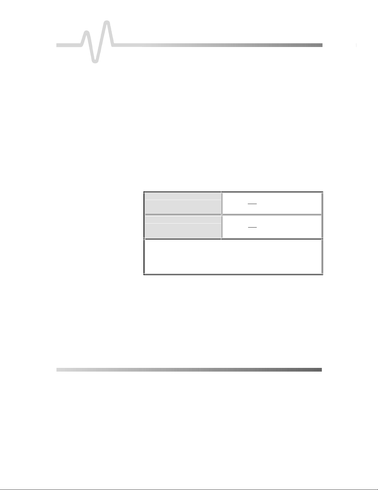
'HWHUPLQLQJ7RSDQG
%DVH/LQHV
Proper determination of the
fundamental for ensuring correct parameter calculations. The
analysis begins by computing a histogram of the waveform data over
the time interval spanned by the left and right time cursors. For
example, the histogram of a waveform trans itioning in two states will
contain two peaks (
two clusters that contain the largest data density. Then the most
probable state (centroids) associated with these two clusters will be
computed to determine the
line corresponds to the top and the
Fig. D–1
top
and
). The analysis will attempt to identify the
top
and
base
base
see below
) is followed by a
page
base
reference lines is
reference levels: the
line to the bottom centroid.
top
maximum
top
LEFT CURSOR
rise
ampl
'²
*not to scale
pkpk
HISTOGRAM*
Lower Threshold
base
minimum
fall
width
Figure D–1
Page 2
$SSHQGL['
'HWHUPLQLQJ5LVHDQG
)DOO7LPHV
Once
top
and
base
are estimated, calculation of the
times is easily done (
Fig.1
). The 90 % and 10 % threshold levels
rise
and
fall
are automatically determined by the oscilloscope, using the
ampl
amplitude (
Threshold levels for
absolute or relative settings (
are chosen, the
) parameter.
rise
or
rise
or
fall
fall
time can also be se lected using
r@level, f@level
). If absolute settings
time is measur ed as the time interval
separating the two crossing points on a rising or falling edge. But
when relative settings are chosen, the vertical interval spanned
base
and
top
between the
lines is subdivided into a percentile
scale (base = 0 %, top = 100 %) to determine the vertical position
of the crossing points.
The time interval separating the points on the rising or falling
edges is then estimated to yield the rise or fall time. These
results are averaged over the number of transition edges that
occur within the observation window.
Mr
1
Rising Edge Duration
Falling Edge Duration
Where Mr is the number of leading edges found, Mf the number of
trailing edges found,
level, and
x
Tf
the time when falling edge i crosses the x % level.
i
x
Tr
the time when rising edge i crosses the x %
i
()
∑
Mr
i
=
1
Mf
1
()
∑
Mf
i
=
1
1090
−
TrTr
ii
9010
−
TfTf
ii
'HWHUPLQLQJ7LPH
3DUDPHWHUV
Time param eter measurements such as
are carried out with respect to the mesial reference level (
), located halfway (50 %) between the top and base
D–2
width, period
and
delay
Fig.
reference lines.
Time-parameter estimation depends on the number of cycles
included within the observation window. If the number of cycles is
rms
or
not an integer, parameter meas urements such as
mean
will be biased.
'²
Page 3
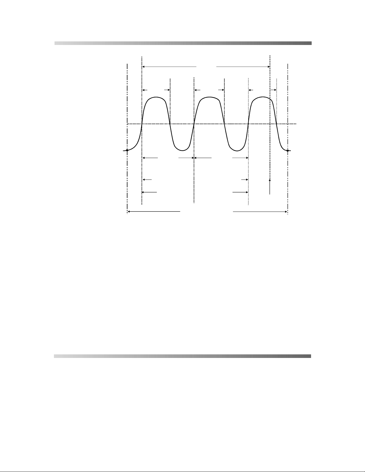
3DUDPHWHU0HDVXUHPHQW
width
delay
50 %
(Mesial)
first
LEFT CURSOR
width
PERIOD PERIOD
freq period
= 1/
TWO FULL PERIODS: = 2
cmean, cmedian, crms, csdev
computed on interval periods
area, points, data
computed between cursors
width
duty width/period
=
cycles
Figure D–2
last
TRIGGER
POINT
RIGHT CURSOR
To avoid these bias effects, the instrument uses cyclic
parameters, including
crms
and
cmean
, that restrict the
calculation to an integer number of cycles.
'HWHUPLQLQJ'LIIHUHQWLDO
7LPH0HDVXUHPHQWV
The oscilloscope enables accurate differential time
measurements between two traces — for example, propagation,
setup and hold delays (
Parameters such as
Fig. D–3
∆
c2d
).
±
require the transition polarity of the
clock and data signals to be specified.
'²
Page 4
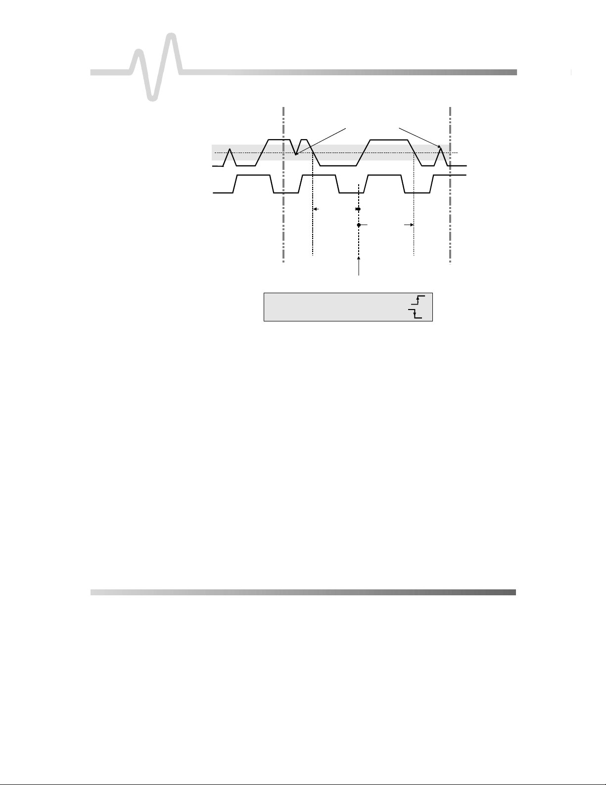
RIGHT CURSOR
DATA (1)
CLK (2)
HYSTERESIS
Noisy spikes ignored due
to Hysteresis band
∆−
c2d (1, 2)
∆
c2d+(1, 2)
$SSHQGL['
THRESHOLD
LEFT CURSOR
CLOCK EDGE = Positive Transition
DATA EDGE = Negative Transition
TRIGGER POINT
Figure D–3
Moreover, a hysteresis range may be specified to ignore any
spurious transition that does not exceed the boundaries of the
∆
c2d
−
hysteresis interval. In Figure 3,
(1, 2) measures the time
interval separating the rising edge of the clock (tr igger) from the
∆
c2d
+
first negative transition of the data signal. Sim ilarly,
(1, 2)
measures the time interval between the trigger and the next
transition of the data signal.
'²
Page 5

3DUDPHWHU0HDVXUHPHQW
3DUDPHWHUDQGZKDWLWGRHV 'HILQLWLRQ 1RWHV
ampl
area
base
cycles
cmean
cmedian
Amplitude: Measures difference between
upper and lower levels in two-level
signals. Differs from
overshoot, undershoot, and ringing do
NOT affect measurement.
Integral of data: Computes area of
waveform between cursors relative to
zero level. Values greater than zero
contribute positively to the area; values
less than zero negatively.
Lower of two most probable states
(higher is
two-level signals. Differs from
noise, overshoot, undershoot, and ringing
do NOT affect measurement.
Determines number of cycles of a
periodic waveform lying between cursors.
First cycle begins at first transition after
the left cursor. Transition may be positiveor negative-going.
Cyclic mean: Computes the average of
waveform data. Contrary to
computes average over an integral
number of cycles, eliminating bias caused
by fractional intervals.
Cyclic median: Computes average of
base and top values over an integral
number of cycles, contrary to
eliminating bias caused by fractional
intervals.
top
). Measures lower level in
pkpk
in that noise,
min
mean
median
in that
,
,
top - base
(See Fig. D–1)
Sum from
last
multiplied by
horizontal time
between points
first
of data
to
(See Fig. D–2)
Value of most
probable lower
state
(See Fig. D–1)
Number of
cycles of
periodic
waveform
(See Fig. D–2)
Average of data
values of an
integral number
of periods
Data value for
which 50 % of
values are above
and 50 % below
On signals
NOT
having two
major levels (such as triangle
or saw-tooth waves), returns
same value as
On signals
pkpk
NOT
having two
major levels (triangle or sawtooth waves, for example),
returns same value as
.
min
.
crms
Cyclic root mean square: Computes
square root of sum of squares of data
values divided by number of points.
Contrary to
over integral number of cycles,
eliminating bias caused by fractional
intervals.
rms
, calculation performed
'²
v
Where:
denotes measured
N
1
∑
N
=
1
i
2
v
()
i
sample values, and
of data points within the periods
found up to maximum of 100
periods.
i
N =
number
Page 6

$SSHQGL['
3DUDPHWHUDQGZKDWLWGRHV 'HILQLWLRQ 1RWHV
csdev
data
delay
∆dly
∆t@lv
∆c2d±
Cyclic standard deviation: Standard
deviation of data values from mean value
over integral number of periods. Contrary
to
sdev
, calculation performed over
integral number of cycles, eliminating
bias caused by fractional intervals.
Returns average of all data points. All data values in
Time from trigger to transition: Measures
time between trigger and first 50 %
crossing after left cursor. Can measure
propagation delay between two signals by
triggering on one and determining delay
of other.
∆delay: Computes time between 50 %
level of two sources.
∆t at level: Computes transition between
selected levels or sources.
∆clock to data ±: Computes difference in
time from clock threshold crossing to either
the next (
∆
c2d
+
) or previous (
∆
c2d
−
) data
threshold crossing.
N
1
−
)meanv(
i
∑
N
=
1
i
analyzed region
(See Fig. D–2)
Time between
trigger and first
50 % crossing
after left cursor
(See Fig. D–2)
Time between
midpoint
transition of two
sources
Time between
transition levels
of two sources,
or from trigger to
transition level of
a single source
Time from clock
threshold
crossing to next
or previous edge
(See Fig. D–3)
Where:
2
sample values, and
v
denotes measured
i
of data points within the periods
found up to maximum of 100
periods.
Multi-value parameter especially
valuable for histograms and
trends.
Reference levels and edgetransition polarity can be
selected. Hysteresis argument
used to discriminate levels
from noise in data.
Threshold levels of clock and
data signals, and edge-transition
polarity can be selected.
Hysteresis argument used to
differentiate peaks from noise in
data, with good hysteresis value
between half expected peak–to–
peak value of signal and twice
expected peak–to–peak value
of noise.
N =
number
'²
Page 7

3DUDPHWHU0HDVXUHPHQW
3DUDPHWHUDQGZKDWLWGRHV 'HILQLWLRQ 1RWHV
dur
duty
f80–20%
f@level
fall
For single sweep waveforms,
sequence waveforms: time from first to
last segment’s trigger; for single
segments of sequence waveforms: time
from previous segment’s to current
segment’s trigger; for waveforms
produced by a history function: time from
first to last accumulated waveform’s
trigger.
Duty cycle: Width as percentage of
period.
Fall 80–20 %: Duration of pulse
waveform's falling transition from 80% to
20%, averaged for all falling transitions
between the cursors.
Fall at level: Duration of pulse waveform's
falling edges between transition levels.
Fall time: Measures time between two
specified values on falling edges of a
waveform. Fall times for each edge are
averaged to produce final result.
Arguments
Threshold Remote Lower
Limit
Lower low 1 % 45 % 10 %
Upper high 55 % 99 % 90 %
Threshold arguments specify two vertical
values on each edge used to compute fall time.
Formulas for upper and lower values:
lower value lower threshold=×+
upper value upper threshold=×+
dur
Upper
Limit
amp
100
amp
100
is 0; for
Default
Time from first to
last acquisition
— for average,
(See Fig. D–2)
Average duration
transition levels
Time at upper
averaged over
each falling edge
(See Fig. D–1)
base
base
histogram or
sequence
waveforms
width/period
of falling
80–20 %
transition
Duration of
falling edge
between
Time at lower
threshold -
threshold
On signals
NOT
having two major
levels (triangle or saw-tooth
waves, for example), top and
base can default to maximum
and minimum, giving, however,
less predictable results.
On signals
NOT
having two major
levels (triangle or saw-tooth
waves, for example), top and
base can default to maximum
and minimum, giving, however,
less predictable results.
NOT
On signals
having two
major levels (triangle or sawtooth waves, for example), top
and base can default to
maximum and minimum,
giving, however, less
predictable results.
'²
Page 8

$SSHQGL['
3DUDPHWHUDQGZKDWLWGRHV 'HILQLWLRQ 1RWHV
first
freq
last
maximum
mean
Indicates value of horizontal axis at left
cursor.
Frequency: Period of cyclic signal
measured as time between every other
pair of 50 % crossings. Starting with first
transition after left cursor, the period is
measured for each transition pair. Values
then averaged and reciprocal used to
give frequency.
Time from trigger to last (rightmost)
cursor.
Measures highest point in waveform.
Unlike
top
, does NOT assume waveform
has two levels.
Average of
waveform. Computed as centroid of
distribution for a histogram. But when
input is periodic time domain waveform,
computed on an integral number of
periods.
data
for time domain
Horizontal axis
value at left
cursor
(See Fig. D–2)
1/
period
(See Fig. D–2)
Time from trigger
to last cursor
(See Fig. D–2)
Highest value in
waveform
between cursors
(See Fig. D–1)
Average of
(See Fig. D–2)
Indicates location of left cursor.
Cursors are interchangeable: for
example, the left cursor may be
moved to the right of the right
cursor and
first
location of the cursor formerly
on the right, now on left.
Indicates location of right cursor.
Cursors are interchangeable: for
example, the right cursor may be
moved to the left of the left cursor
first
will give the location of
and
the cursor formerly on the left,
now on right.
Gives similar result when
applied to time domain
waveform or histogram of
of same waveform. But with
histograms, result may include
contributions from more than
one acquisition. Computes
horizontal axis location of
rightmost non-zero bin of
histogram — not to be
confused with
data
Gives similar result when
maxp
applied to time domain
waveform or histogram of
of same waveform. But with
histograms, result may include
contributions from more than
one acquisition.
will give the
data
.
data
'²
Page 9

3DUDPHWHU0HDVXUHPHQW
3DUDPHWHUDQGZKDWLWGRHV 'HILQLWLRQ 1RWHV
median
minimum
over−
over+
period
pkpk
phase
points
The average of base and top values. Average of
(See Fig. D–2)
Measures the lowest point in a waveform.
Unlike
base
, does NOT assume waveform
has two levels.
Lowest value in
waveform
between cursors
(See Fig. D–1)
base minimum
−
Overshoot negative: Amount of overshoot
following a falling edge, as percentage of
16
ampl
amplitude.
(See Fig. D–2)
maximum top
Overshoot positive: Amount of overshoot
following a rising edge specified as
16
ampl
percentage of amplitude.
(See Fig. D–1)
Period of a cyclic signal measured as
time between every other pair of 50 %
crossings. Starting with first transition
after left cursor, period is measured for
Mr
Mr
1
∑
i
=
each transition pair, with values averaged
to give final result.
(See Fig. D–2)
Peak–to–peak: Difference between
highest and lowest points in waveform.
maximum
minimum
Unlike ampl, does not assume the
waveform has two levels.
Phase difference between signal analyzed
and signal used as reference.
(See Fig. D–1)
Phase difference
between signal
and reference
Number of points in the waveform between
the cursors.
Number of points
between cursors
(See Fig. D–2)
base
and
top
Gives similar result when
applied to time domain
waveform or histogram of data
of same waveform. But with
histograms, result may include
contributions from more than
one acquisition.
least one falling edge. On
NOT
signals
having two major
Waveform must contain at
100
×
levels (triangle or saw-tooth
waves, for example), may
give predictable results.
−
Waveform must contain at
100
×
least one rising edge. On
NOT
signals
having two major
levels (triangle or saw-tooth
waves, for example), may
give predictable results.
Where:
leading edges found, Mf the
()
1
5050
−
TrTr
number of trailing edges
ii
found,
edge
and
edge
-
Gives a similar result when applied
Mr
is the number of
x
Tr
the time when rising
i
i
crosses the x % level,
x
Tf
the time when falling
i
i
crosses the x % level.
to time domain waveform or
histogram of data of the same
waveform. But with histograms,
result may include contributions
from more than one acquisition.
NOT
NOT
'²
Page 10

$SSHQGL['
3DUDPHWHUDQGZKDWLWGRHV 'HILQLWLRQ 1RWHV
r20–80%
r@level
rise
Rise 20 % to 80 %: Duration of pulse
waveform’s rising transition from 20% to
80%, averaged for all rising transitions
between the cursors.
Rise at level: Duration of pulse
waveform's rising edges between
transition levels.
Rise time: Measures time between two specified
values on waveform’s rising edge (10–90 %).
Rise times for each edge averaged to give final
result.
Arguments
Thr es h ol d Remote
Lower low 1 % 45 % 10 %
Lower
Limit
Upper
Limit
Default
Average duration
of rising 20–80 %
transition
Duration of rising
edges between
transition levels
Time at upper
threshold - Time at
lower threshold
averaged over each
rising edge
(See Fig. D–1)
On signals
NOT
having two
major levels (triangle or sawtooth waves, for example), top
and base can default to
maximum and minimum,
giving, however, less
predictable results.
On signals
NOT
having two
major levels (triangle or sawtooth waves, for example), top
and base can default to
maximum and minimum,
giving, however, less
predictable results.
On signals
NOT
having two
major levels (triangle or sawtooth waves, for example), top
and base can default to
maximum and minimum,
giving, however, less
predictable results.
Upper high 55 % 99 % 90 %
Threshold arguments specify two vertical values
on each edge used to compute rise time.
Formulas for upper and lower values:
amp
lower value lower threshold=×+
upper value upper threshold=×+
100
amp
100
base
base
'²
Page 11

3DUDPHWHU0HDVXUHPHQW
f
3DUDPHWHUDQGZKDWLWGRHV 'HILQLWLRQ 1RWHV
rms
Root Mean Square of data between the
cursors — about same as
sdev
for a
zero-mean waveform.
N
1
N
∑
=
i
v
()
1
(See Fig. D–2)
Gives similar result when applied to
2
time domain waveform or histogram
i
of data of same waveform. But with
histograms, result may include
contributions from more than one
acquisition.
v
Where:
values, and
denotes measured sample
i
N =
number of data
points within the periods found up to
maximum of 100 periods.
sdev
t@level
top
width
Standard deviation of the data between
the cursors — about the same as
rms
for
a zero-mean waveform.
Time at level: Time from trigger (t=0) to
crossing at a specified level.
Higher of two most probable states, the lower
being
base
. This is characteristic of rectangular
waveforms and represents the higher most
probable state determined from the statistical
distribution of
data
point values in the waveform.
Width of cyclic signal determined by examining
50 % crossings in data input. If first
transmission after left cursor is a rising edge,
waveform is considered to consist of positive
pulses and
width
the time between adjacent
rising and falling edges. Conversely, if falling
edge, pulses are considered negative and
width
the time between adjacent falling and
rising edges. For both cases, widths of all
waveform pulses averaged for final result.
N
1
−
)meanv(
i
∑
N
=
1
i
(See Fig. D–2)
Time from trigger
to crossing level
Value of most
probable higher
state
(See Fig. D–1)
Width of first
positive or
negative pulse
averaged for all
similar pulses
(See Figs. 1, 2)
Gives similar result when applied to
2
time domain waveform or histogram
of data of same waveform. But with
histograms, result may include
contributions from more than one
acquisition.
v
Where:
sample values, and
denotes measured
i
N =
number o
data points within the periods found
up to maximum of 100 periods.
Gives similar result when
applied to time domain
waveform or histogram of
of same waveform. But with
histograms, result may include
contributions from more than
one acquisition.
fwhm
Similar to
, which,
however, applies only to
histograms.
data
'²
 Loading...