Lecroy 93XXC-OM-E21 User Manual

&

$SSHQGL[&)DVW)RXULHU7UDQVIRUP))7

:KHQDQG+RZWR8VH))7

The WP02 Spectral Analysis package, with FFT (Fast Fourier
Transform), reveals signal characteristics not visible in t he
time domain and adds the power of frequency domain
analysis to your oscilloscope. FFT converts a time domain
waveform into frequency domain spectra similar to those of
a spectrum analyzer, but with important differences and
added benefits.

:K\8VH))7" For a large class of signals, greater insight can be gained by

looking at spectral representation rather than time description.
Signals encountered in the frequency response of amplifiers,
oscillator phase noise and those in mechanic al vibration analysis

— to mention just som e applications — are easier to observe in
the frequency domain.

If sampling is done at a rate f ast enough to f aithfully approxim ate
the original waveform (usually five times the highest frequency
component in the signal), the resulting discrete data series will
uniquely describe the analog signal.

This is of particular value when dealing with transient signals
because, unlike FFT, conventional swept spectrum analyzers
cannot handle them.

7KHRU\%HKLQG))7 Spectral analysis theory assumes that the signal for

transformation be of infinite duration. Since no physical signal
can meet this condition, a useful assumption for reconciling
theory and practice is to view the signal as consisting of an
infinite series of replica of itself . Thes e replica are m ultiplied by a
rectangular window (the display grid) that is zero outside of the
observation grid.

À

For an explanation of FFT terms: see the Glossary

on page C–17

À

Using FFT Functions: see page C–9

À

FFT Algorithms: page C–14

&²

$SSHQGL[&

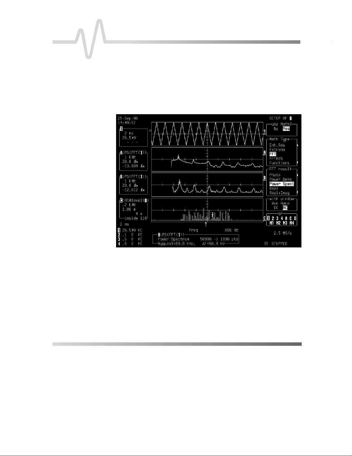
Figure C–1 shows spectra of a swept triangular wave.
Discontinuities at the edges of the wave produce leakage, an
effect clearly visible in Trace A, which was computed with a
rectangular window, but less pronounced in the Von Hann
window in Trace B (

explanations

first harmonic.

). Histogramming in Trace C tracks the spread of the

see below for leakage and window-type

Figure C–1

Slicing the waveform in the fashion described above is
tantamount to diluting the spectral energy in an infinite number of
side lobes, which correspond to multiples of the frequency
resolution ∆f (
T determines the frequency resolution of the FFT (∆f=1/T).
Whereas the sampling period and the record length set the
maximum frequency span that can be obtained (f

Fig. C–2

&²

). The observation window or capture time

=∆f*N/2).

Nyq

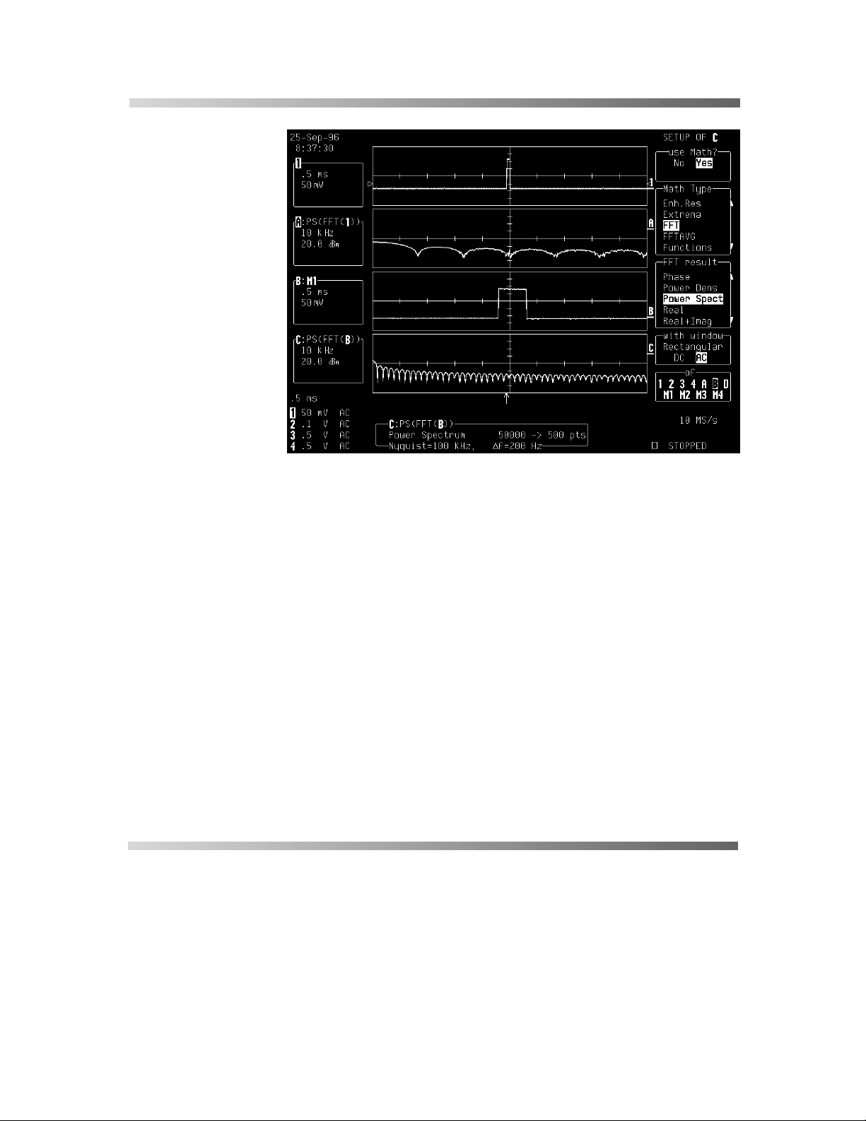
Figure C–2

8VLQJ))7

An FFT operation on an N point time-dom ain signal may thus be
compared to passing the signal through a comb f ilter consisting
of a bank of N/2 filters. All the filter s have the same shape and
width and are centered at N/2 discrete frequencies. Each filter
collects the signal energy that falls into the immediate
neighborhood of its center frequency. Thus it can be said that
there are N/2 frequency bins. The distance in Hz between the
center frequencies of two neighboring bins is always the same:

∆

f.

3RZHU'HQVLW\6SHFWUXP Because of the linear scale used to show magnitudes, lower

amplitude components are often hidden by larger com ponents . In
addition to the functions offering magnitude and phase
representations, the FFT option offers power density and power

spectrum density functions, selec ted from the “FFT result” m enu
shown in the figures. These latter functions are even better
suited for characterizing spectra. The power spectr um (V

2

) is the
square of the magnitude spectrum (0 dB m corresponds to
voltage equivalent to 1 mW into 50 Ω.) This is the representation

&²

$SSHQGL[&

of choice for signals containing isolated peaks — periodic
signals, for instance.

2

The power density spectrum (V
divided by the equivalent noise bandwidth of the filter in Hz
associated with the FFT calculation. This is best employed for
characterizing broad-band signals such as noise.

0HPRU\IRU))7 The amount of acquisition memory available will determine the

maximum range (Nyquist frequency) over which signal
components can be observed. Consider the problem of
determining the length of the observation window and the size of
the acquisition buffer if a Nyquist rate of 500 MHz and a
resolution of 10 kHz are required. To obtain a resolution of 10
kHz, the acquisition time must be at least:

T = 1/∆f = 1/10 kHz = 100 µs.

For a digital oscilloscope with a memory of 100 k, the highest
frequency that can be analyzed is:

∆f ×

N/2 = 10 kHz × 100 k/2 = 500 MHz.

/Hz) is the power spectrum

))73LWIDOOVWR$YRLG Take care to ensure that signals are correctly acquired: im proper

waveform positioning within the observation window produces a
distorted spectrum. T he most com mon distortions can be trac ed
to insufficient sampling, edge discontinuities, windowing or the
“picket fence” effect.

Because the FFT acts like a bank of bandpass filters c entered at
multiples of the frequency resolution, components that are not
exact multiples of that frequency will fall within two consecutive
filters. This results in an attenuation of the true amplitude of
these components.

3LFNHW)HQFHDQG6FDOORS The highest point in the spectrum c an be 3.92 dB lower when the

source frequency is halfway between two discrete frequencies.
This variation in spectrum magnitude is the picket fence effect.
And the corresponding attenuation loss is ref erred to as scallop
loss. LeCroy scopes automatically correc t for the scallop effect,
ensuring that the magnitude of the spectra lines correspond to
their true values in the time domain.

&²

8VLQJ))7

If a signal contains a frequency component above Nyquist, the
spectrum will be aliased, meaning that the frequencies will be
folded back and spurious. Spotting aliased frequencies is of ten
difficult, as the aliases may ride on top of real harmonics. A
simple way of checking is to modify the sample rate and verify
whether the frequency distribution changes.

/HDNDJH FFT assumes that the signal contained within the time grid is

replicated endlessly outside the observation window. Therefore if
the signal contains discontinuities at its edges, pseudo­frequencies will appear in the spectral dom ain, distorting the real
spectrum. W hen the start and end phas e of the signal differ, the
signal frequency falls within two frequency cells broadening the
spectrum.

This effect is illustrated in Figure C–1. Bec ause the display does
not contain an integral number of periods, the spectrum
displayed in Trace B does not reveal sharp frequency
components. Intermediate components exhibit a lower and
broader peak. The broadening of the base, stretching out in
many neighboring bins, is termed leakage. Cures for this are to
ensure that an integral number of periods is contained within the
display grid or that no discontinuities appear at the edges.
Another is to use a window function to smooth the edges of the
signal.

&KRRVLQJD:LQGRZ The choice of a spectral window is dictated by the signal’s

characteristics. Weighting functions control the filter response
shape and affect noise bandwidth as well as side-lobe levels.
Ideally, the main lobe should be as narrow and flat as possible to
effectively discriminate all spectral components, while all side
lobes should be infinitely attenuated.

Chosen from the “with window” menu, the window type defines
the bandwidth and shape of the equivalent filter to be used in the
FFT processing.

In the same way as one would choose a particular camera lens
for taking a picture, s ome experimenting is generally necessary
to determine which window is most suitable. However, the
following general guidelines should help (

window types

).

&²

see page C–11 for

$SSHQGL[&

Rectangular windows provide the highest frequency resolution
and are thus useful for estim ating the type of harm onics pres ent
in the signal. Because the rectangular window decays as a sinx/x
function in the spectral domain, slight attenuation will be induced.

Alternative functions with less attenuation — Flat-top and
Blackman-Harr is — provide maximum amplitude at the expense
of frequency resolution. Whereas, Hamming and von Hann are
good for general purpose use with continuous waveforms.

,PSURYLQJ'\QDPLF5DQJH Enhanced resolution (

technique that can potentially provide for three additional bits
(18 dBs) if the signal noise is uniformly distributed (white). Low
pass filtering should be considered when high frequency
components are irrelevant. A distinct advantage of this technique
is that it works for both repetitive and transient signals. The SNR
increase is conditioned by the cut-off frequency of the Eres low
pass filter and the noise shape (frequency distribution).

LeCroy digital oscilloscopes employ FIR digital filters so that a
constant phase shift is maintained. The phase information is
therefore not distorted by the filtering action.

6SHFWUDO3RZHU$YHUDJLQJ Even greater dynamic-range im provem ent is obtained on signals

showing periodicity. Moreover, the range can be increased
without sacrificing frequency response. T he LeCroy oscilloscope
being used is equipped with accumulation buffers 32 bits wide to
prevent overflows.

Spectral power averaging is useful when the signal var ies in tim e
and the mean power of the signal needs to be estim ated. T ypical
applications include noise and pseudo- random noise. Whereas
time averaging ignores phase information, spectral averaging
tracks magnitude as well as phase information. It is thus a
superior estimator. And the improvement is typically proportional
to the square root of the number of averages. For instance,
averaging white noise at full scale over 10 sweeps yields a typical
improvement of nearly 20 dBs.

see Appendix B

) uses a low pass f iltering

&²

8VLQJ))7

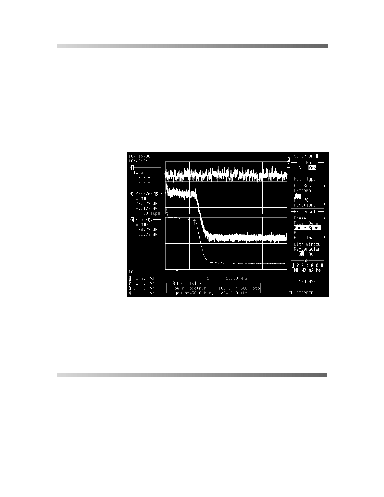
Spectral power averaging is the technique of choice when
determining the frequency response of passive network s suc h as
filters. Figures 3 and 4 show the transfer functions of a low pass
filter with a 3 dB cutoff o1 11 MHz obtained by exciting the filter
with a white noise source (
(

Fig. C–4

The choice of method is governed by the availability of an
adequate generating source.

The spectra of single tim e-domain waveforms can be computed
and displayed to obtain power averages obtained over as many
as 50 000 spectra.

). Both techniques give substantially the same results.

Fig. C–3

) and a sine swept generator

&²

Figure C–3