

Page 1
Operator’s Manual
LeCroy
9300C Series
Digital Oscilloscopes
Revision A — January 1998
Page 2
LeCroy Corporation
700 Chestnut Ridge Road
Chestnut Ridge, NY 10977–6499
Tel: (845) 578 6020, Fax: (845) 578 5985
LeCroy SA
2, rue du Pré-de-la-Fontaine
1217 Meyrin 1/Geneva, Switzerland
Tel: (41) 22 719 21 11, Fax: (41) 22 782 39 15
Internet: www.lecroy.com
Copyright © January 1998, LeCroy. All rights reserved. Information in this publication supersedes all
earlier versions. Specifications subject to change.
LeCroy, ProBus and SMART Trigger are registered trademarks of LeCroy Corporation. MathCad is
a registered trademark of MATHSOFT Inc. Centronics is a registered trademark of Data Computer
Corp. Epson is a registered trademark of Epson America Inc. PowerPC is a registered trademark of
IBM Microelectronics. MATLAB is a registered trademark of The MathWorks, Inc. DeskJet,
ThinkJet, QuietJet, LaserJet, PaintJet, HP 7470 and HP 7550 are registered trademarks of HewlettPackard Company. I
Manufactured under
an ISO 9000
Registered
Quality Management
System
Visit www.lecroy.com
to view the certificate.
2
C is a trademark of Philips.
This electronic product is
subject to disposal and
recycling regulations that
vary by country and
region. Many countries
prohibit the disposal of
waste electronic
equipment in standard
waste receptacles.
For more information
about proper disposal
and recycling of your
LeCroy product, please
visit
www.lecroy.com/recycle.
93XXC-OM-E Rev A 0198
Page 3
Chapter 1 — Read This First!
Product and Client Care..............................................................1–1
Chapter 2 — Instrument Architecture
General Designed Capabilities................................................2–1
Block Diagrams.................................................................................2–4
Chapter 3 — Installation and Safety
Installation for Safe and Efficient Operation...................3–1
Chapter 4 — Introduction to the Controls
The Front Panel.................................................................................4–1
The Main Controls.......................................................................... 4–3
Choosing and Navigating in Menus.......................................4–4
System Setup and Menu Controls..........................................4–6
Screen Topography ........................................................................4–8
Contents
Chapter 5 — CHANNELS, Coupling and Probes
Channel Controls..................................................................... 5–1
Coupling...............................................................................................5–3
Probes and Probe Calibration ..................................................5–4
Chapter 6 — TIMEBASE + TRIGGER
TIMEBASE + TRIGGER Controls..............................................6–1
Chapter 7 — Timebase Modes and Setup
Timebase Sampling Modes........................................................7–1
Timebase Setup ...............................................................................7–5
iii
Page 4

Chapter 8 — Triggers and When to Use Them
Choosing the Right Trigger .......................................................8–1
Edge or SMART? ..............................................................................8–2
Edge Trigger ......................................................................................8–3
TRIGGER SETUP: Edge................................................................8–9
SMART Triggers.............................................................................8–10
TRIGGER SETUP: SMART ........................................................ 8–29
Chapter 9 — ZOOM + MATH
Zoom and Math Controls............................................................. .9–1
Chapter 10 — Zoom, Mathematics and Math Setup
Zooming for Precise Waveform Measurements...........10–1
Math Functions and Options ..............................................10–2
Using Waveform Mathematics...........................................10–5
Configuring for Zoom and Math.........................................10–6
Setting Up FFT Span and Resolution .............................10–17
Contents
Chapter 11 — Display
Chapter 12 — UTILITIES
Setting Up the Display........................................................ 11–1
Printing, Storing, Using Special Modes ........................... 12–1
Hardcopy Setup............................................................................12–2
Time/Date Setup...........................................................................12–4
GPIB/RS232 Setup.......................................................................12–5
Mass Storage Utilities .............................................................. 12–7
Special Modes ........................................................................ 12–19
CAL BNC Setup.............................................................................12–21
iv
Page 5

Chapter 13 — WAVEFORM STORE & RECALL
Waveform Store......................................................................13–1
Waveform Recall....................................................................13–4
Chapter 14 — CURSORS/MEASURE & Parameters
Cursors: Tools for Measuring Signal Values.................14–1
Parameters: Automatic Measurements ..........................14–4
Pass/Fail Testing...................................................................14–13
Chapter 15 — PANEL SETUPS
Saving and Recalling Panel Setups...............................15–1
Chapter 16 — SHOW STATUS
The Complete Picture — Summarized............................ 16–1
Appendix A — Specifications
Appendix B — Enhanced Resolution
Appendix C — Fast Fourier Analysis (FFT)
Appendix D — Parameter Measurement
Appendix E — ASCII-Stored Files
v
Page 6
1
Read This First!
Product and Client Care
We recommend you thoroughly inspect the contents of the
scope packaging at once. Check all the contents against
the packing list/invoice copy shipped with the instrument
and the list on page 1–3 of this manual. Unless LeCroy is
notified promptly of a missing or damaged item, we cannot
accept responsibility for its replacement. Contact your
national LeCroy Customer Service Department or local
office immediately (contact numbers follow index).
Warranty LeCroy warrants its oscilloscope products for normal use and
operation within specifications for a period of three years from
the date of shipment. Calibration each year is recommended to
ensure in-spec performance. Spares, replacement parts and
repairs are warranted for 90 days. The instrument's firmware has
been thoroughly tested and is thought to be functional, but is
supplied without warranty of any kind covering detailed
performance. Products not made by LeCroy are covered solely
by the warranty of the original equipment manufacturer.
In exercising its warranty, LeCroy will repair or, at its option,
replace any product returned within the warranty period to the
Customer Service Department or an authorized service center.
However, this will be done only if the product is determined by
LeCroy’s examination to be defective due to workmanship or
materials, and the defect has not been caused by misuse,
neglect or accident, or by abnormal conditions or operation.
Note: This warranty replaces all other warranties,
expressed or implied, including but not limited to any
implied warranty of merchantability, fitness, or adequacy
for any particular purpose or use. LeCroy shall not be liable
for any special, incidental, or consequential damages,
whether in contract or otherwise. The client will be
responsible for the transportation and insurance charges
for the return of products to the service facility. LeCroy will
return all products under warranty with transport prepaid.
1–1
Page 7

Read This First!
Product Assistance Help on installation, calibration, and the use of LeCroy
equipment is available from the LeCroy Customer Service
Department in your country (see contact numbers following the
index).
Maintenance Agreements We provide a variety of customer support services. Maintenance
agreements give extended warranty and allow our clients to
budget maintenance costs after the initial three-year warranty
has expired. Other services such as installation, training,
enhancements and on-site repairs are available through special
Supplemental Support Agreements.
Staying Up to Date LeCroy is dedicated to offering state-of-the-art instruments,
continually refining and improving the performance of our
products. Because of the speed with which physical
modifications may be implemented, this manual and related
documentation may not agree in every detail with the products
they describe. For example, there might be small discrepancies
in the values of components affecting pulse shape, timing or
offset, and — infrequently — minor logic changes.
However, be assured the scope itself is in full order and
incorporates the most up-to-date circuitry.
We frequently update firmware or software during servicing to
improve scope performance, free of charge during warranty. We
will keep you up to date with such changes, through new or
revised manuals and other publications.
But you should retain this, the original manual, for future
reference to your scope’s unchanged hardware
specifications.
Service and Repair Please return products requiring maintenance to the Customer
Service Department in your country or to an authorized service
facility. LeCroy will repair or replace any product under warranty
free of charge. The customer is responsible for transportation
charges to the factory, whereas all in-warranty products will be
returned to you with transportation prepaid. Outside the warranty
period, you will need to provide us with a purchase order
number before we can repair your LeCroy product. You will be
1–2
Page 8

billed for parts and labor related to the repair work, and for
shipping.
1–3
Page 9
Read This First!
How to Return a ProductContact your country’s Customer Service Department or local
field office to find out where to return the product. All returned
products should be identified by model and serial number. You
should describe the defect or failure, and provide your name
and contact number. And in the case of products returned to the
factory, a Return Authorization Number (RAN) should be used.
The RAN can be obtained by contacting the Customer Service
Department.
Return shipments should be made prepaid. We cannot accept
COD (Cash On Delivery) or Collect Return shipments. We
recommend air-freighting.
It is important that the RAN be clearly shown on the outside of
the shipping package for prompt redirection to the appropriate
LeCroy department.
What Comes with Your Scope The following items are shipped
together with the standard configuration of this oscilloscope:
Ø Front Scope Cover
Ø 10:1 10 MΩ Passive Probe — one per channel
Ø ProBus Single-Channel Adapter (9354C, 9374C, 9384C
SERIES ONLY)
Ø Two 250 V T-rated Fuses (5 A or 6.3 A depending on model
— see Chapter 3)
Ø AC Power Cord and Plug
Ø Operator’s Manual (this manual)
Ø Remote Control Manual
Ø Hands-On Guide
Ø Performance Certificate
Ø Declaration of Conformity
Ø Warranty
Note: Wherever possible, please use the original shipping
carton. If a substitute carton is used, it should be rigid and
packed so that that the product is surrounded by a minimum
of four inches or 10 cm of shock-absorbent material.
1–4
Page 10

2
Instrument
Architecture
General Designed Capabilities
Your oscilloscope is the newest
version of a series that set the
standard for monochrome DSOs
(Digital Storage Oscilloscopes).
Each of the scope’s channels has an
8-bit ADC (Analog–to–Digital Converter).
On the higher-range models, combining two channels doubles
the scope’s sampling rate. While on high-range, four-channel
models, combining all channels increases the original rate by
four times.
Processors The central microprocessor performs the scope’s computations and
controls its operation. A wide range of peripheral interfaces allow
remote control, storage and printing. A support processor constantly
monitors the front-panel controls, rapidly reconfiguring setups. Data
processing is also rapid, with data being transferred to the display
memory for direct waveform display or stored in the reference
memories (see below).
Note: Wherever a feature is specific to a particular model,
or not included with a model, it is indicated thus:
9314C ONLY, for example.
For the complete list of specifications for each
model, see the section on that model or its series in
Appendix A.
ADCs The instrument’s multiple-ADC architecture ensures absolute
amplitude and phase correlation, maximum ADC performance for
multi-channel acquisitions, large record lengths and excellent time
resolution.
Memories The copious acquisition memories simplify transient capture by
producing long waveform records that capture even when triggertiming or signal-speed is uncertain. Combining channels also
increases the acquisition memory length. There are four memories
for temporary storage, and four more for waveform zooming and
processing.
2–1
Page 11

Instrument
Architecture
RIS Repetitive signals can be acquired and stored at a Random
Interleaved Sampling (RIS) rate of 10 GS/s. RIS is a highprecision digitizing technique that enables measurement of
repetitive signals to the instrument's full bandwidth, with an
effective sampling interval of 100 ps and measurement
resolution of 10 ps. (See Chapter 7).
Trigger System The Trigger System offers an extensive range of capabilities,
selected according to the character of the signal, using onscreen menus and front-panel controls. In standard trigger mode
these menus and controls enable the selection and setting of
parameters such as pre- and post-trigger recording, as well as
special modes. The trigger source can be any of the input
channels, line (synchronized to the scope’s main input supply) or
external. The coupling is selected from AC, LF REJect, HF
REJect, HF, and DC; the slope from positive and negative. (See
Chapter 8.)
Automatic Calibration The oscilloscope’s automatic calibration ensures an overall
vertical accuracy of typically 1% of full scale. Vertical gain and
offset calibration take place each time the volts/div setting is
modified. In addition, periodic calibration is performed to ensure
long-term stability at the current setting.
Display System The display’s interactive, user-friendly interface is controlled by
push-buttons and knobs (see Chapter 4).
The large, 12.5 × 17.5 cm (nine-inch diagonal) screen shows
waveforms and data with enhanced resolution on a variety of
grid styles (see Chapter 11). Up to four waveforms can be
displayed at once, while the parameters controlling signal
acquisition are simultaneously reported. The screen presents
internal status and measurement results, as well as operational,
measurement, and waveform-analysis menus.
Printing or copying the screen on plotter, printer or to a
recording medium is done by pressing the front-panel SCREENDUMP button(See Chapter 12).
2–2
Page 12

Manual or Remote
Control
Despite being a truly digital instrument, the scope has a frontpanel layout and controls that will be familiar to users of analog
oscilloscopes. Rapid instrument response and instant
representation of waveforms on the high-resolution screen add
to this impression.
Four front-panel setups can be stored internally and recalled
either manually or by remote control, thus ensuring rapid frontpanel configuration. When the power is switched off, the current
front-panel settings are automatically stored for subsequent
recall at the next power-on.
The oscilloscope has also been designed for remote control
operation in automated testing and computer-aided
measurement applications — operations described in the
Remote Control Manual. The entire measurement process,
including cursor and pulse-parameter settings, dynamic
modification of front-panel settings, and display organization, is
controlled through the rear-panel GPIB (IEEE-488) and
RS-232-C ports (see Chapter 12).
2–3
Page 13
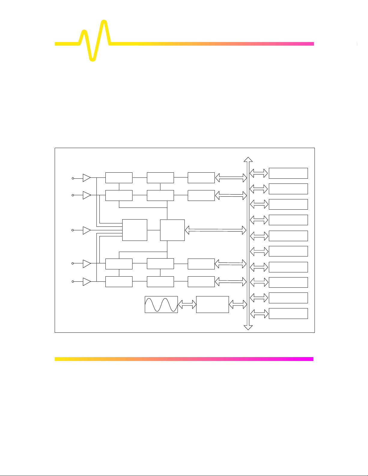
Block Diagrams
Program memory
Microprocessor
Storage devices
Ø 9304C, 9310C, 9314C
Instrument
Architecture
Series
Hi-Z, 50 Amplifiers + Attenuators
CH1
CH2
External
trigger
CH3
CH4
W
Sample
& Hold
Sample
& Hold
Sample
& Hold
Sample
& Hold
Trigger
logic
8-bit
Flash ADC
8-bit
Flash ADC
Timebase
8-bit
Flash ADC
8-bit
Flash ADC
Fast
memory
Fast
memory
Fast
memory
Fast
memory
processor
Display
Centronics
RS-232-C
GPIB
Coprocessor
Front-panel
processor
Real-time
clock
Data memories
2–4
Page 14
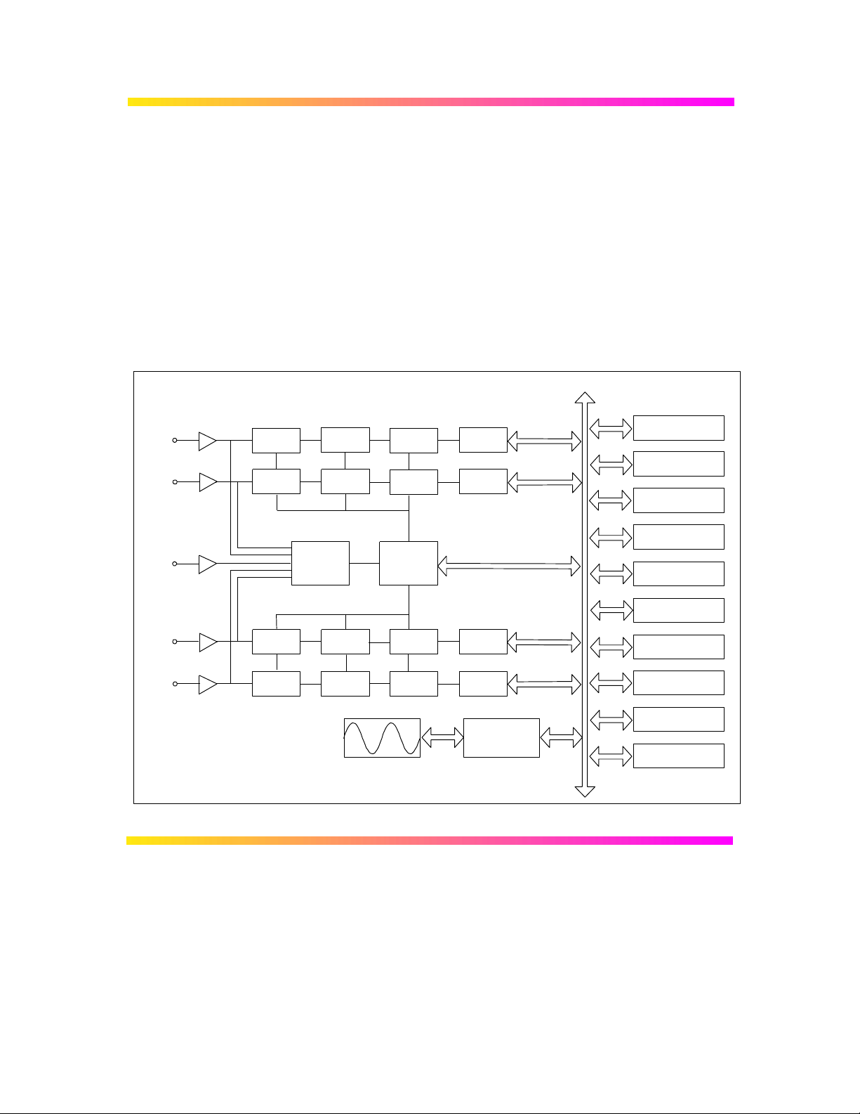
Ø 9344C, 9350C, 9354C
Program memory
Microprocessor
Series
Ø 9370C, 9374C Series
Ø 9384C Series
Hi-Z, 50 Amplifiers + Attenuators
CH1
CH2
External
trigger
CH3
CH4
W
Sample
& Hold
Sample
& Hold
Sample
& Hold
Sample
& Hold
8-bit ADC
8-bit ADC
Trigger
logic
8-bit ADC
8-bit ADC
Peak
detect
Peak
detect
Timebase
Peak
detect
Peak
detect
Fast
memory
Fast
memory
Fast
memory
Fast
memory
Display
processor
Storage devices
Centronics
RS-232-C
GPIB
Coprocessor
Front-panel
processor
Real-time
clock
Data memories
2–5
Page 15
3
Installation and Safety
Installation for Safe and Efficient Operation
The oscilloscope will operate to its specifications if the
operating environment is maintained within the following
parameters:
Operating Environment
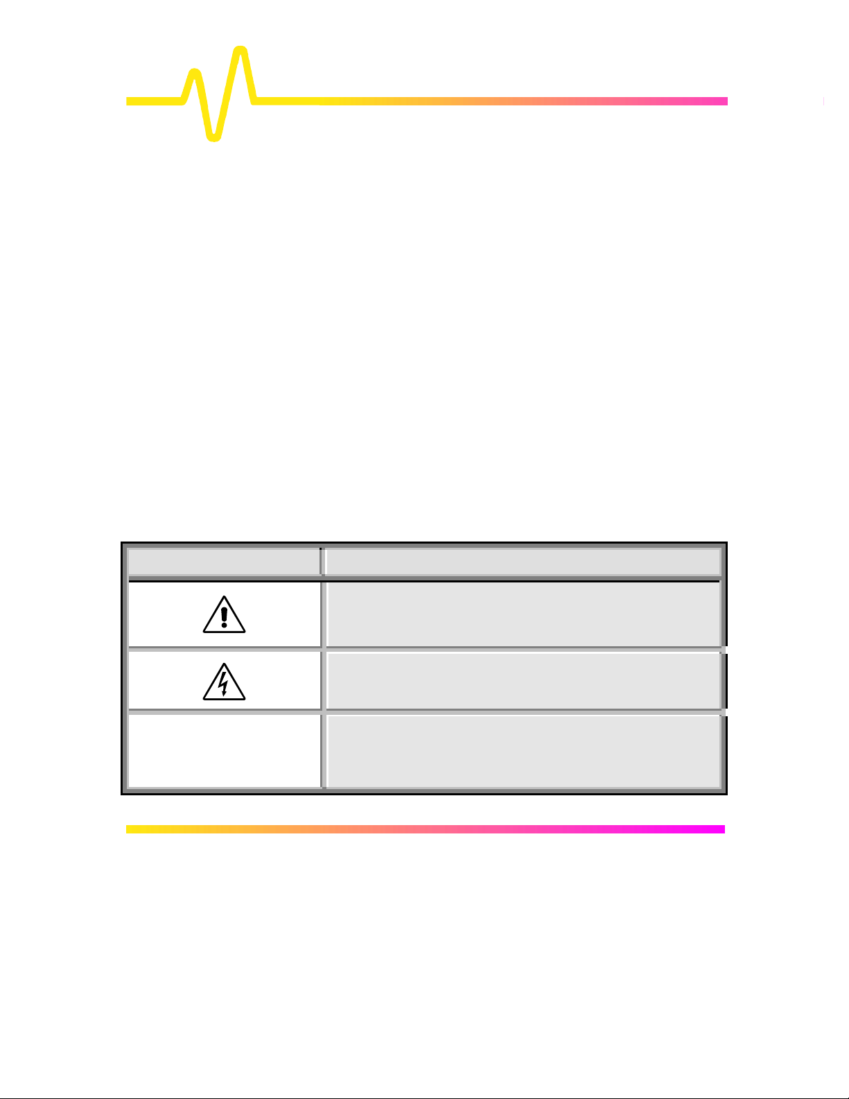
Safety Symbols Where the following symbols or indications appear on the
Symbol Meaning
Ø Temperature..........................5 to 40 °C (41 to 104 °F) rated.
Ø Humidity................................Maximum relative humidity 80 % RH
(non-condensing) for temperatures up
to 31 °C decreasing linearly to 50 %
relative humidity at 40 °C
Ø Altitude ..................................< 2000 m (6560 ft)
The oscilloscope has been qualified to the following EN61010-1
category:
Ø Protection Class.........................................I
Ø Installation (Overvoltage) Category...........II
Ø Pollution Degree.........................................2
instrument’s front or rear panels, or elsewhere in this manual, they
alert the user to an aspect of safety.
CAUTION: Refer to accompanying documents (for Safetyrelated information).
See elsewhere in this manual wherever the symbol is present,
as indicated in the Table of Contents.
CAUTION: Risk of electric shock.
x
On (Supply).
3–1
Page 16

Installation and Safety
Symbol Meaning
Off (Supply)
Earth (Ground) Terminal
Protective Conductor Terminal
Chassis Terminal
Earth (Ground) Terminal on BNC Connectors
Denotes a hazard. If a WARNING is indicated on the
WARNING
WARNING Any use of this instrument in a manner not specified by the
Power RequirementsThe oscilloscope operates from a 115 V (90 to 132 V) or 220 V (180
instrument, do not proceed until its conditions are
understood and met.
manufacturer may impair the instrument’s safety
protection. The oscilloscope has not been designed to
make direct measurements on the human body. Users who
connect a LeCroy oscilloscope directly to a person do so at
their own risk. Use only indoors.
to 250 V) AC power source at 45 Hz to 66 Hz.
3–2
Page 17

No voltage selection is required, since the instrument automatically
adapts to the line voltage present.
Fuses The oscilloscope’s power supply is protected against short-circuit and
overload by means of two “T”-rated fuses of type according to scope
model:
Ø 6.3 A/250 V AC 9344C, 9350C, 9354C, 9370C, 9374C, 9384C Series
Ø 5 A/250 V AC 9304C, 9310C, 9314C Series.
The fuses are located above the mains plug. Disconnect the power
cord before inspecting or replacing a fuse. Open the fuse box by
inserting a small screwdriver under the plastic cover and prying it open.
For continued fire protection at all line voltages, replace only with fuses
of the specified type and rating (see above).
Ground The oscilloscope has been designed to operate from a single-phase
power source, with one of the current-carrying conductors (neutral
conductor) at ground (earth) potential. Maintain the ground line to
avoid an electric shock. None of the current-carrying conductors
may exceed 250 V rms with respect to ground potential. The
oscilloscope is provided with a three-wire electrical cord containing a
three-terminal polarized plug for mains voltage and safety ground
connection. The plug's ground terminal is connected directly to the
frame of the unit. For adequate protection against electrical hazard,
this plug must be inserted into a mating outlet containing a safety
ground contact.
Cleaning and Maintenance Maintenance and repairs should be carried out exclusively by a LeCroy
technician (see Chapter 1). Cleaning should be limited to the exterior of
the instrument only, using a damp, soft cloth. Do not use chemicals or
abrasive elements. Under no circumstances should moisture be allowed
to penetrate the oscilloscope. To avoid electric shocks, disconnect the
instrument from the power supply before cleaning.
CAUTION Risk of electrical shock: No user-serviceable parts inside. Leave
repair to qualified personnel.
Power On Connect the oscilloscope to the power outlet and switch it on by pressing
the power switch located on the rear panel. After the instrument is
switched on, auto-calibration is performed and a test of the
oscilloscope's ADCs and memories is carried out. The full testing
procedure takes approximately 10 seconds, after which time a display
will appear on the screen.
3–3
Page 18
4
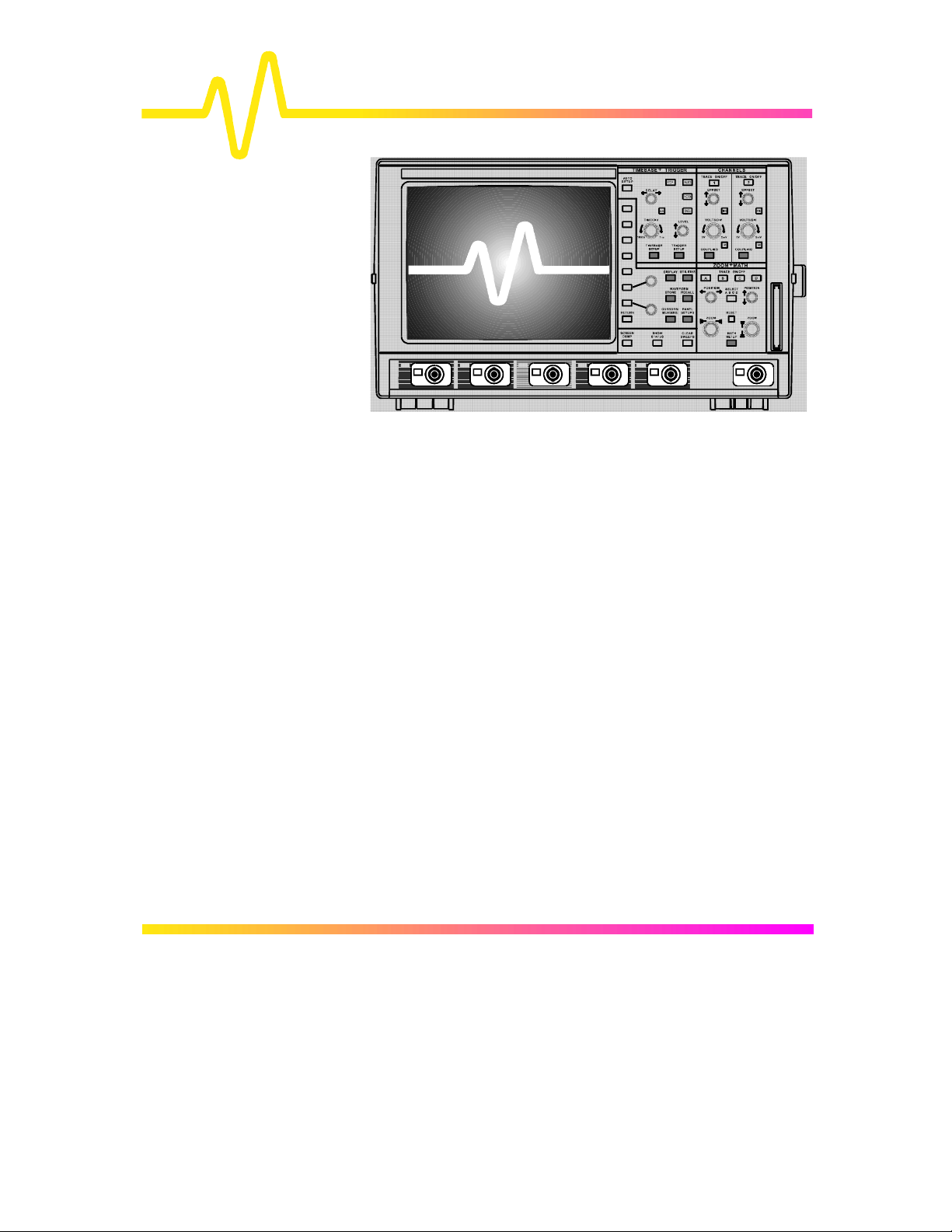
Two-Channel Front Panel
Introduction to the
Controls
4–1
Page 19

Four-Channel Front Panel
Introduction to the
Controls
4–2
Page 20
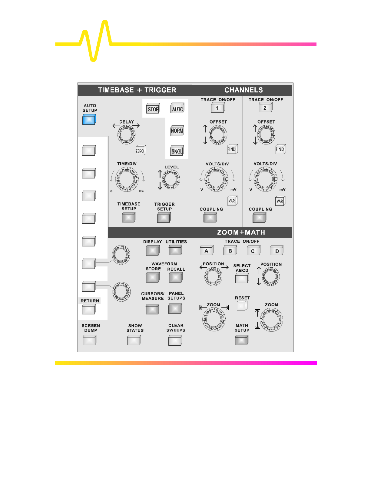
The Main Controls
The front panel controls are divided into four main groups
of buttons and knobs: the System Setup and menu
controls, CHANNELS, TIMEBASE + TRIGGER and ZOOM +
MATH.
System Setup Dark-gray, menu-entry buttons, also represented in the other
groups of controls, provide access to the main on-screen menus
and the acquisition, processing and display modes of the
instrument.
The SCREEN DUMP, SHOW STATUS and CLEAR SWEEPS
buttons, respectively: copy or print the screen display, show onscreen summaries of the scope’s status, and restart operations that
require several acquisitions. See page 4–6.
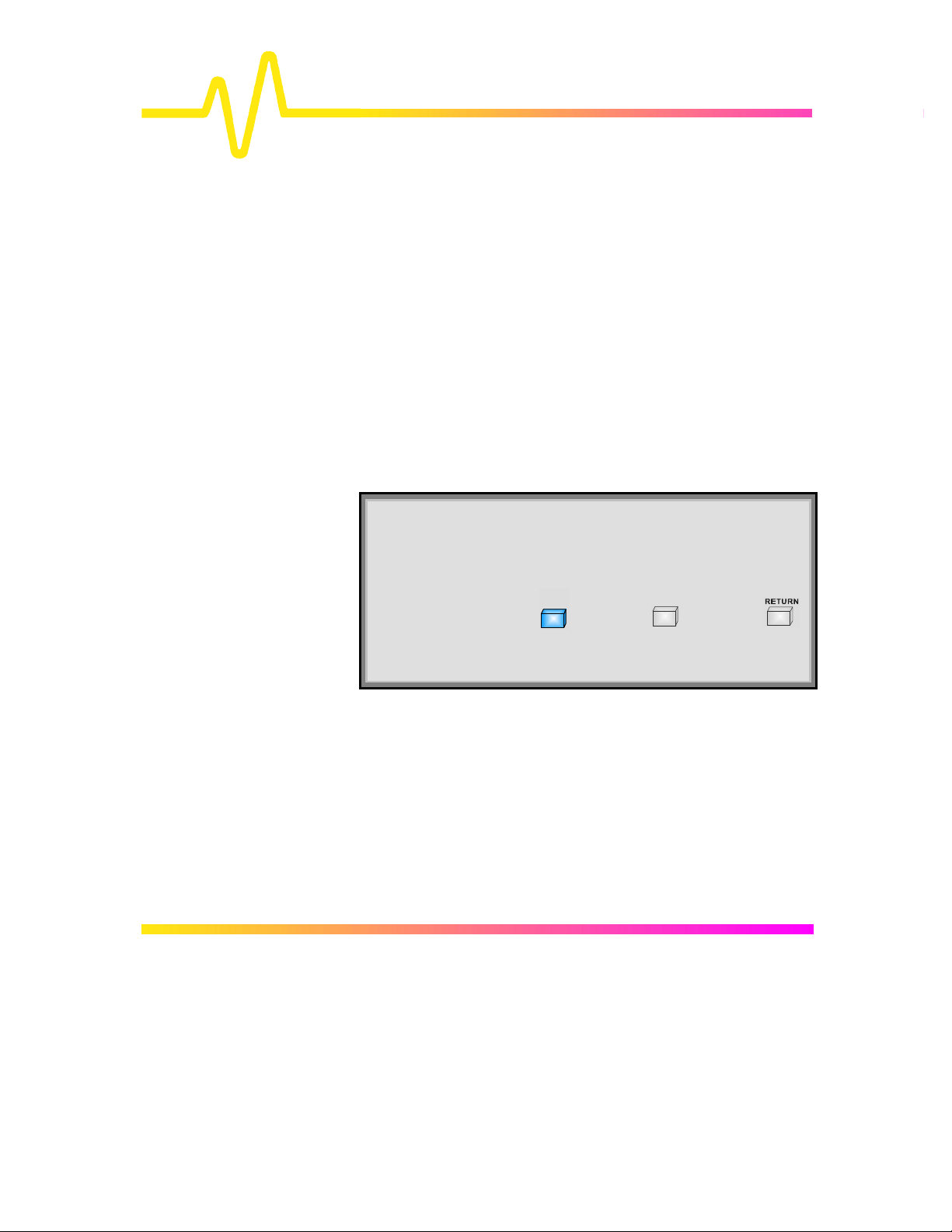
Menu Buttons & Knobs The seven untitled buttons vertically aligned beside the screen,
RETURN and the two linked rotary knobs enable on-screen menu
selection. See following pages.
CHANNELS This group offers selection of displayed traces and adjustment of
vertical sensitivity and offset. See Chapter 5.
AUTO SETUP This singular blue button automatically adjusts the scope to acquire
and display signals on the input channels. See Chapter 6.
TIMEBASE + TRIGGER These controls allow direct adjustment of time/division, trigger level
and delay, as well as access to the “TIMEBASE” and “TRIGGER”
menu groups. See Chapters 6, 7 and 8.
ZOOM + MATH And this group controls trace selection, movement, definition, and
expansion with Zoom and Math functions. See Chapters 9 and 10.
See also “ Getting Started”, Part 2 of the
Hands-On Guide , for more on the front-panel
and a complete run-through of the controls…
4–3
Page 21
Introduction to the
entry
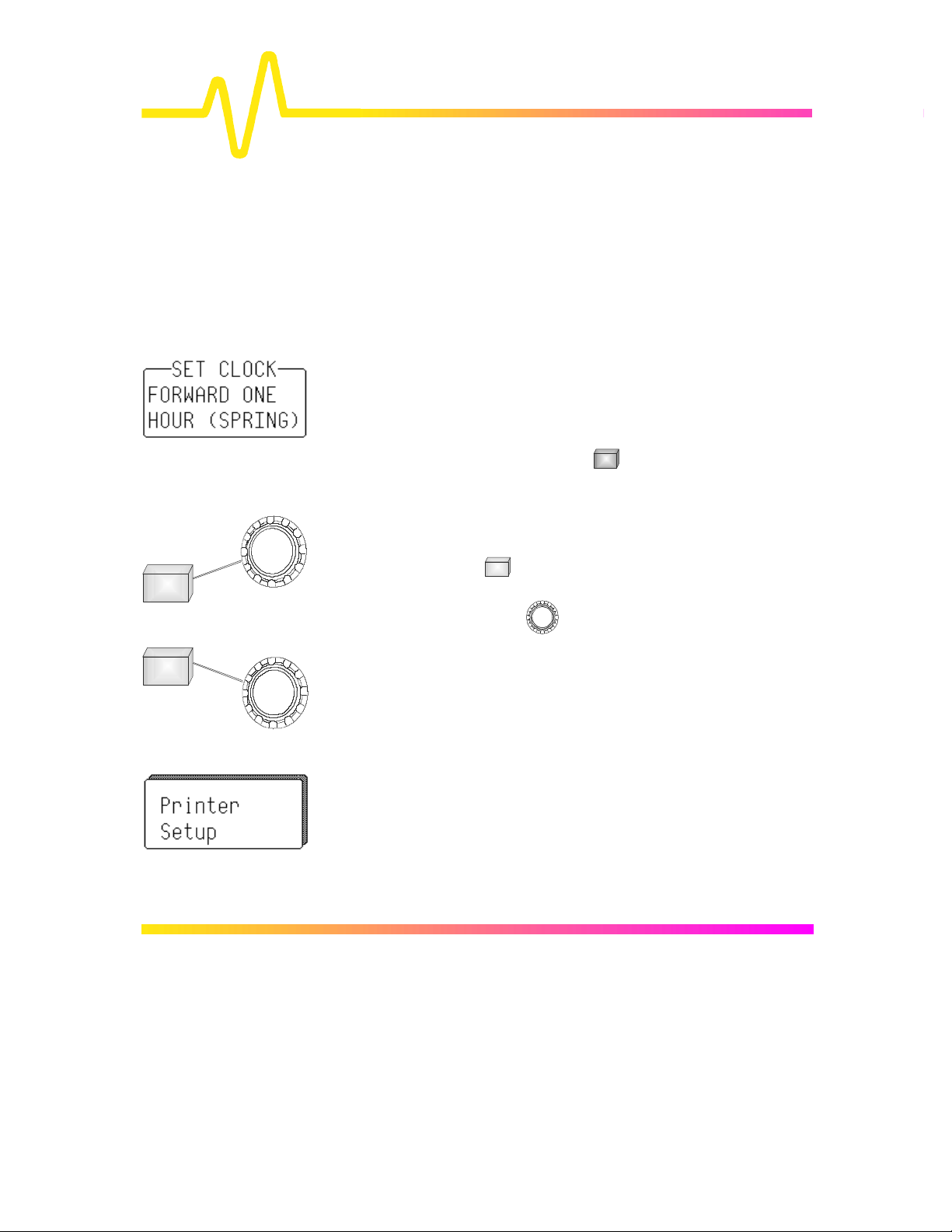
Choosing and Navigating in Menus
On-screen menus — the panels running down the righthand side of the screen — are used to select specific scope
actions and settings. All other on-screen text is for
information only. The menus are broadly grouped
according to function. The name of each menu group is
shown at the top of the column of menus. Individual menus
also have names in the top of their frames.
Each menu either contains a list of items or options — functions
to be selected or variables modified — or when selected
performs a specific action. Menus that perform certain actions
are indicated by capitalized text, as in the example shown at left.
Controls
Going to Menus and
Selecting from them
When a menuconfiguration for its particular group of functions is immediately
displayed on-screen as a menu group. Once accessed, these
menus are controlled using the menu buttons and the two menu
knobs (illustrated at left).
A menu button is active and can be pressed to make
selections whenever a menu is visible beside it on-screen.
The two menu knobs work together with the two menu
buttons to which they are joined by lines. Both control the
menus currently shown beside them. Buttons and knobs are
used either for selecting entire menus, particular items from
menus, for moving up or down through menu lists, or for
changing the values listed in menus.
Some menus, referred to as primary, have secondary menus
beneath them whose existence is indicated by a heavy outline or
shadow, as illustrated at left. Pressing the corresponding menu
button reveals and activates these ‘hidden’ menus. Pressing the
RETURN button again displays the top, or primary, menu.
Changing a menu value normally changes the screen, because the
new value is immediately used in acquisition settings, processing or
display.
button is pressed, the set-up
4–4
Page 22
Setting Menu Options The activated selection is highlighted in the menu. Press the
corresponding menu button and the field will advance to
highlight and select the next item on the menu. However, if
there is only one item on a menu, pressing its button will have
no effect.
Where a menu is associated with one of the two menu knobs,
turning this knob in one direction or the other will cause the
selection to move either up or down the list in the menu.
Menus that extend along the length of two menu buttons can be
operated using both buttons. Pressing the lower of the two will
move the highlighting forward — down the list — while pushing
the upper will move the selector back up the list.
An arrow on the side of a menu frame indicates that by pressing
the button beside this arrow, the selection can be moved further
up or down the list. The arrow’s direction shows whether the
highlighting selector will move up or down. Arrows may also
indicate items that are not visible, either above or below on the
list. The respective arrow will disappear when the selection is at
the very beginning or end of the list.
As in the examples at left, some menu button and knob
combinations control the value of a continuously adjustable
variable. The knob is then used to set its value, while the button
either selects a value or makes a simple change in it.
Still other menu button and knob combinations control the value
of several continuously adjustable variables, with the knob used
to set the value and the button to highlight it.
Note: When the oscilloscope is placed in a remote state,
the REMOTE ENABLE menu will be displayed. It will
contain the command “GO TO LOCAL”, activated by menu
button if the action is possible. This is the only manual
way to turn off the REMOTE ENABLE menu. The scope
need not be in remote state to accept remote commands.
4–5
Page 23
Introduction to the
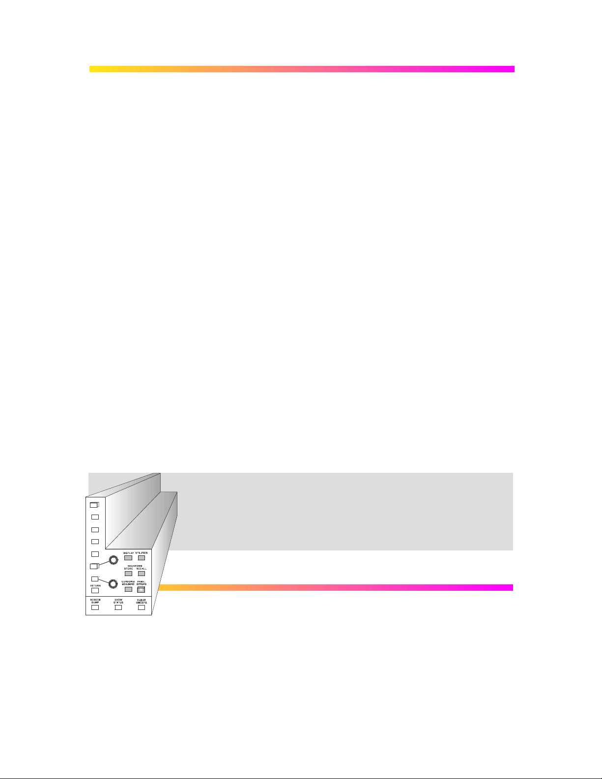
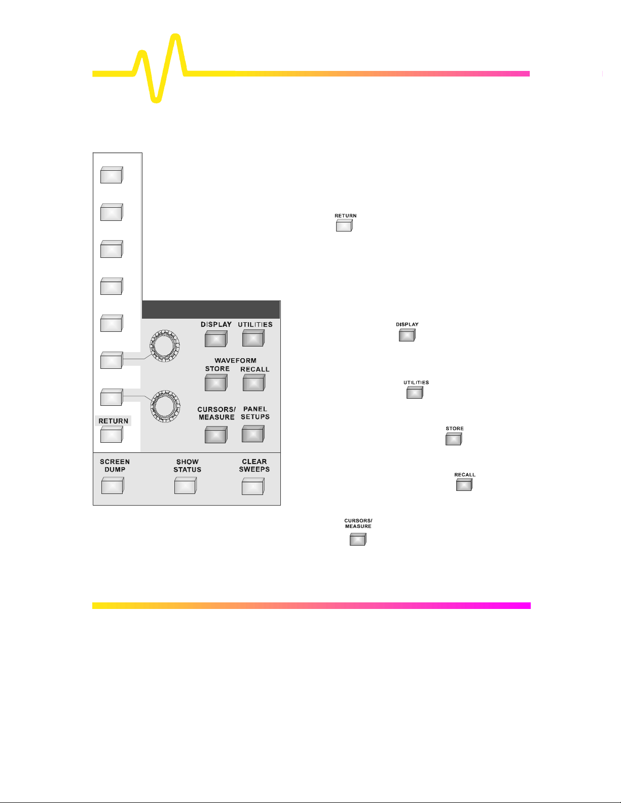
System Setup and Menu Controls
As well as the menu buttons and knobs described on the
previous pages, the System Setup controls include the menuentry buttons and others for copying displays, reporting
instrument status and restarting multiple-acquisition
operations.
The RETURN button is used to go back to the preceding
displayed menu group. Or it returns the display to a higher-level, or
primary menu. But when the display is at the highest possible menu
level, the button switches off that menu.
Each of the dark-gray menu-entry buttons activates a major set of
on-screen menus (those represented in the other control groups are
described in the following chapters, along with the other
elements in the groups).
The DISPLAY button provides entry to the
“DISPLAY SETUP” group of menus, controlling display
mode, grids, intensities, Dot Join and Persistence menus.
See Chapter 11.
Controls
The UTILITIES button gives access to the
“UTILITIES” menus, controlling hardcopy setups, GPIB
addresses and special modes of operation. Chapter 12.
The WAVEFORM STORE button
“STORE W’FORM” menus, used for storing waveforms
to internal or external memory. Chapter 13.
Whereas, WAVEFORM RECALL
“RECALL W’FORM”: menus for retrieving waveforms
stored in internal or external memory. Chapter 13.
CURSORS/MEASURE
menus, used for making precise cursor measurements on traces,
and “MEASURE”, for precise parameter measurements. Chapter
14.
4–6
offers up the “CURSORS” Setup
accesses the
calls up
Page 24

And PANEL SETUPS gives access to the “PANEL SETUPS”
menus for saving and recalling a configuration of the instrument.
See Chapter 13.
SCREEN DUMP — prints or plots the screen display to an on-line hardcopy device,
via the GPIB, RS-232-C or Centronics interface ports, or directly to
an external thermal graphics printer. Hardcopies can also be
generated as data files onto floppy, memory card or portable hard
disk.
Once SCREEN DUMP is pressed, all displayed information will be
copied. However, it is possible to copy the waveforms without the
grid by turning the grid intensity to 0 with the “Display Setup” menu.
While a screen dump is taking place — indicated by the on-screen
“PRINTING” or “PLOTTING” message — it can be aborted by
pressing SCREEN DUMP a second time. It will take a certain
amount of time for the buffer to empty before copying stops.
CLEAR SWEEPS — restarts operations requiring several acquisitions, or sweeps,
including averaging, extrema, persistence and pass/fail testing, by
resetting the sweep counter(s) to zero.
SHOW STATUS — menu entry to “STATUS”, which shows summaries of the
instrument’s status for acquisition, system and other aspects. See
Chapter 16.
4–7
Page 25
Screen Topography
Introduction to the
Controls
The sections of the screen shown here and described below, which surround the grid,
contain a variety of useful information as well as accessing specific commands and functions.
4–8
Page 26
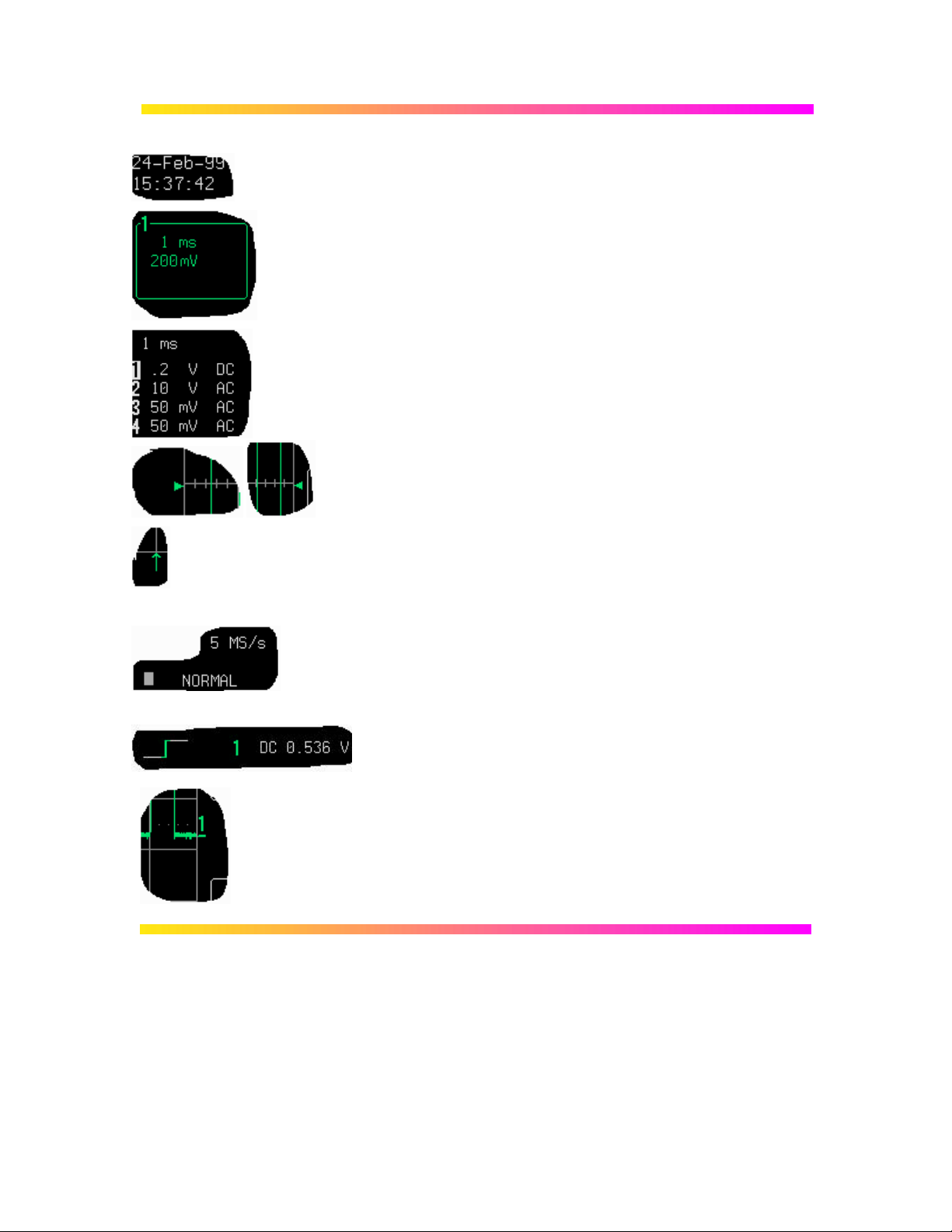
Real-Time Clock field: powered by a battery-backed real-time
clock, it displays the current date and time.
Displayed Trace Label indicates each channel or channel
displayed, the time/div and volts/div settings, and cursor
readings where appropriate. It indicates the acquisition
parameters set when the trace was captured or processed, while
the Acquisition Summary field (below) indicates the present
setting.
Acquisition Summary field: timebase, volts/div, probe
attenuation and coupling for each channel, with the selected
channel highlighted. It indicates the present setting, while the
acquisition parameters set when the trace was captured or
processed are indicated in the Displayed Trace label (above).
Trigger Level arrows on both sides of the grid that mark the
trigger voltage level relative to ground level.
Trigger Delay: an arrow indicating the trigger time relative to
the trace. The delay can be adjusted from zero to ten grid
divisions (pre-trigger), or zero to −10 000 (post-trigger) offscreen. Pre-trigger delay appears as the upward-pointing arrow,
while post-trigger is given as a delay in seconds.
Trigger Status field shows sample rate and trigger re-arming
status (AUTO, NORMAL, SINGLE, STOPPED). The small
square icon flashes to indicate that an acquisition has been
made.
Trigger Configuration field: icon indicating type of trigger, and
information on the trigger’s source, slope, level and coupling,
and other information when appropriate.
Trace and Ground Level: trace number and ground-level
marker.
4–9
Page 27
Introduction to the
AUTO
SETUP
Controls
Other Fields
(not illustrated here)
Time and Frequency field: displays time and frequency relative
to cursors beneath the grid. For example, when the absolute
time cursor (the cross-hair) is activated by selection from the
“MEASURE” menu group, this field displays the time between
the cursor and the trigger point.
Message field: used to display a variety of messages, above
the grid, including warnings, indications and titles showing the
instrument’s current status.
General Instrument Reset: Simultaneously
press the AUTO SETUP button, the top menu
button, and the RETURN button. The scope will
revert to its default power-up settings.
Press:
!
+ +
4–10
Page 28
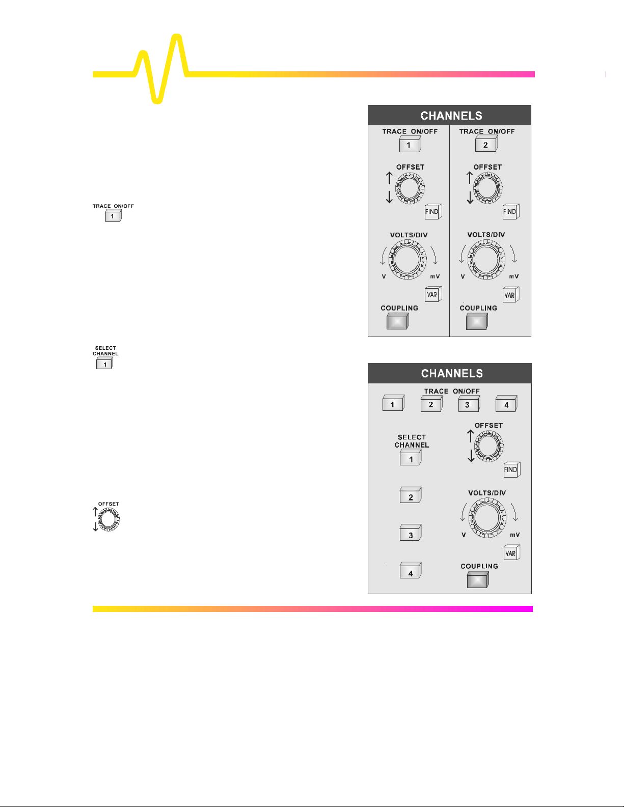
5
Channel Controls
These enable selection
of displayed traces and
adjustment of vertical
sensitivity and offset.
TRACE ON/OFF Pressing these buttons either
displays or switches off the
corresponding channel trace.
When a channel is switched
on, the OFFSET and
VOLTS/DIV controls will
then be attributed to this, the
active channel. On twochannel models (right), each
channel has its own set of
unique, dedicated controls.
CHANNELS, Coupling & Probes
SELECT CHANNEL On four-channel models
(right), these buttons are
used to attribute all the
vertical controls to one
channel, independent of
whether or not it is the
channel displayed. The
selected channel number
is highlighted in the
Acquisition Summary
field (see previous
chapter).
OFFSET — vertically positions the
active channel.
5–1
Page 29
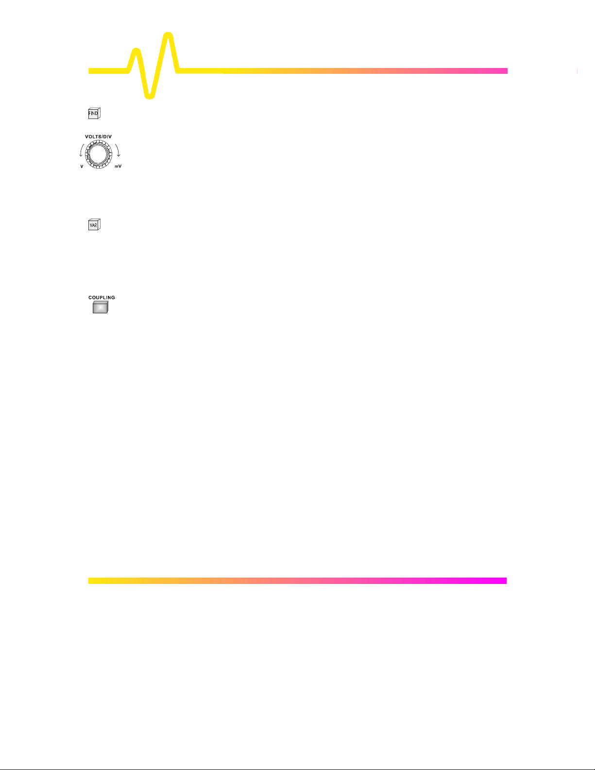
CHANNELS, Coupling & Probes
FIND — automatically adjusts offset and volts/div to match the active
channel’s input signal.
VOLTS/DIV — selects the vertical sensitivity factor either in a 1–2–5 sequence
or continuously (see VAR, below ). The effect of gain changes on the
acquisition offset can be chosen from the “SPECIAL MODES”
menu.
VAR — allows the user to determine whether the VOLTS/DIV knob will
modify the vertical sensitivity in a continuous manner or in discrete
1–2–5 steps.
The format of the vertical sensitivity in the Acquisition Summary
field (bottom left of screen) shows whether the VOLTS/DIV knob is
operating in continuous or stepping mode.
COUPLING — menu-entry button that accesses the “Coupling” menus (see next
section).
5–2
Page 30
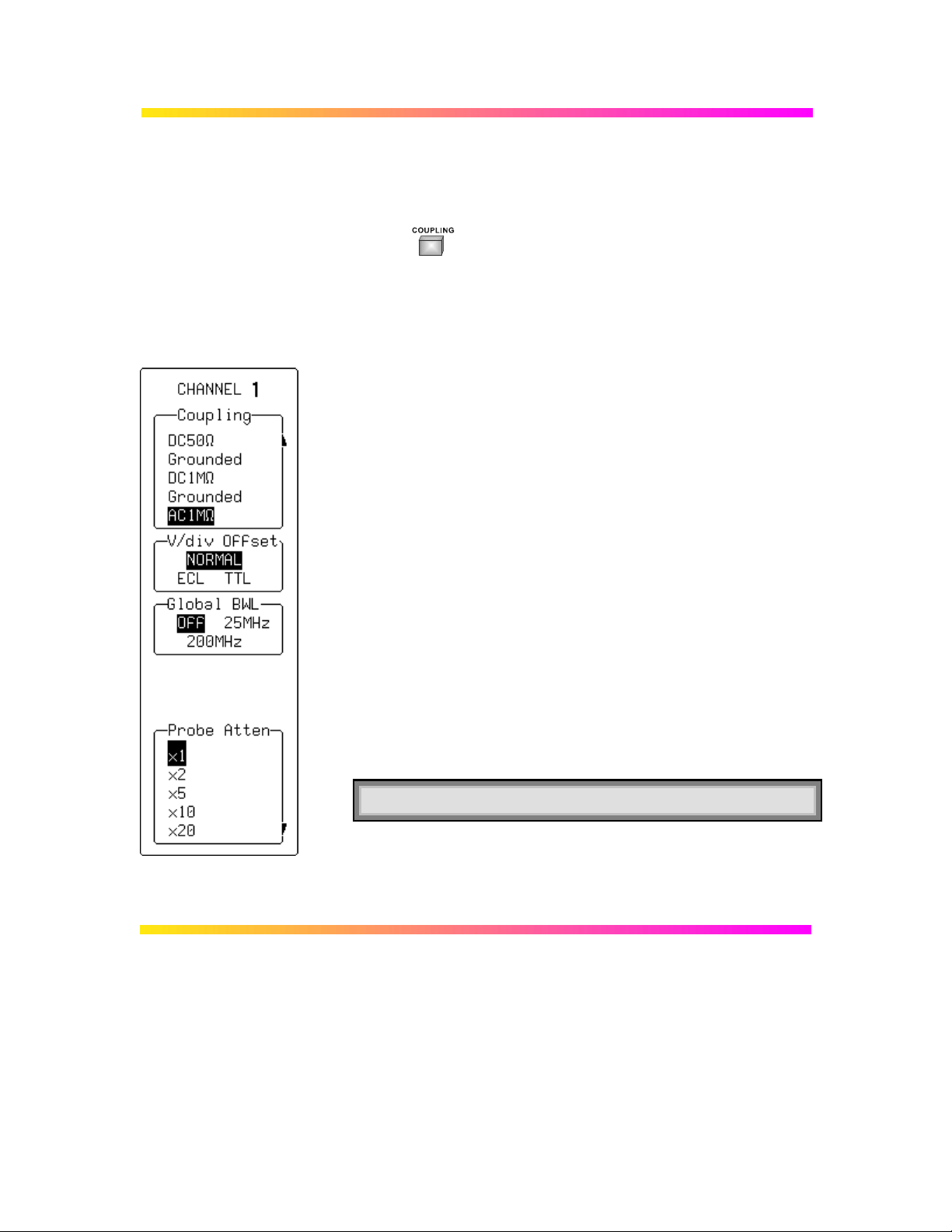
Coupling
Coupling Menus Press for access to selection of:
Ø Coupling and grounding of each input channel
Ø ECL or TTL gain, offset and coupling preset for the
channel shown
Ø Bandwidth limiter for all channels
Ø Probe attenuation of each input channel.
Coupling
Used to select the input channel’s coupling. If an overload is
detected, the instrument will automatically set the channel to the
grounded state: the menu can then be reset to the desired coupling.
V/div Offset
When NORMAL is highlighted, pressing the corresponding menu
button sets the offset, Volts/div, and input coupling to display ECL
signals. Press the button a second time and the settings for TTL
signals are given. And a third time returns the settings to those used
at the last manual setup of the channel.
Global BWL
To turn the bandwidth limit “OFF” or “ON”. The bandwidth can be
reduced from 500 MHz or 1 GHz, to either 200 MHz or 25 MHz, or
30 MHz (–3dB), depending on the model (see Appendix A).
Bandwidth limiting can be useful in reducing signal and system
noise or preventing high-frequency aliasing, reducing — for
example — any high-frequency signals that may cause aliasing in
single-shot applications.
Note: This command is global and affects all input channels.
Probe Atten
Sets the probe attenuation factor related to the input channel (see
following for probe details).
5–3
Page 31

CHANNELS, Coupling & Probes
In the AC position, signals are coupled capacitively, thus
blocking the input signal’s DC component and limiting the
In the DC position, all signal frequency components are
allowed to pass through, and 1
MΩ or 50
Ω may be chosen as
The maximum dissipation into 50
Ω is 0.5
W and inputs will
automatically be grounded whenever this is attained. An
overload message will be displayed in the Acquisition
Summary Field and “Grounded” will be indicated in the
the signal from the input and again selecting the 50
Ω input
Probes and Probe Calibration
Probe Calibration To calibrate the probe supplied, connect it to one of the input
channels’ BNC connectors. Connect the probe’s grounding
alligator clip to the CAL BNC ground and touch the tip to the
inner conductor of the CAL BNC. The CAL signal is a 1 kHz
square wave, 1 V p-p.
Set the channel coupling to DC 1 MΩ, turn the trace ON and
push AUTO SETUP to set up the oscilloscope. If over- or
undershoot of the displayed signal occurs, the probe can be
adjusted by inserting the small screwdriver, supplied with the
probe package, into the trimmer on the probe’s barrel and
turning it clockwise or counter-clockwise to achieve the optimal
square-wave contour.
More On Coupling
signal frequencies below 10 Hz.
the input impedance.
“Coupling” menu. The overload condition is reset by removing
impedance from the menu.
5–4
Page 32

ProBus System LeCroy’s ProBus system provides a complete measurement
solution from probe tip to oscilloscope display. This intelligent
interconnection between LeCroy oscilloscopes and a growing range
of accessories is achieved via a six-wire bus following Philips’ I2C
protocol. It provides major benefits over standard BNC or even
probe-ring connections:
Ø Autosensing the probe type, eliminating all the guesswork —
and the errors — from manually setting attenuation or
amplification factors, and ensuring proper input coupling.
Ø Transparent gain and offset control right from the front panel
— particularly useful for FET (FET menus shown here) and
current probes.
Ø Gain and offset correction factors are uploaded from the
ProBus EPROMS on FET probes and automatically
compensated to achieve fully calibrated measurements.
Coupling
Used to select the input channel’s coupling. If an overload is
detected, the instrument will automatically set the channel to the
grounded state: the menu can then be reset to the desired coupling.
V/div Offset
When NORMAL is highlighted, pressing the corresponding menu
button sets the offset, Volts/div, and input coupling to display ECL
signals. Press the button a second time and the settings for TTL
signals are given. And a third time returns the settings to those used
at the last manual setup of the channel.
Global BWL
To turn the bandwidth limit “OFF” or “ON”. The bandwidth can be
reduced from 500 MHz or 1 GHz, to either 200 MHz or 25 MHz, or
30 MHz (–3dB), depending on the model (see Appendix A).
Bandwidth limiting can be useful in reducing signal and system
noise or preventing high-frequency aliasing, reducing — for
example — any high-frequency signals that may cause aliasing in
single-shot applications.
When a FET probe is used, “Probe sensed…”, automatically
appears to indicate settings. When other ProBus probes are
used, this is redefined.
5–5
Page 33

6
TIMEBASE + TRIGGER
TIMEBASE + TRIGGER Controls
These controls allow direct adjustment of time/division,
trigger level and delay, and access the “TIMEBASE” and
“TRIGGER” menu groups.
AUTO SETUP The blue button
automatically scales
the timebase, trigger
level, offset, and
volts/div to provide a
stable display of
repetitive signals.
AUTO SETUP operates only on
channels which are active. If no
channels are on, then AUTO
SETUP will operate on all
channels, switching them all on.
Signals detected must have an
amplitude between 5 mV and
40 V, a frequency greater than
50 Hz, and a duty cycle greater
than 0.1 %.
If signals are detected on several channels, the channel with the
lowest number will determine the selection of the timebase and
trigger source.
STOP This button halts the acquisition in any of the three re-arming
modes: Auto, Normal or Single.
Pressing the STOP button prevents the oscilloscope acquiring a
new signal.
Press STOP while a single-shot (see next chapter) acquisition is
under way and the last acquired signal will be kept.
6–1
Page 34

TIMEBASE + TRIGGER
Press STOP after an RIS acquisition has been started (next
chapter) and the acquisition will be halted and a partial
waveform reconstruction will be performed.
Press STOP when the acquisition is in Roll Mode (see next
chapter) and the incomplete acquisition data will be shown as if
a trigger had occurred.
In Sequence Mode (next chapter), the action will stop the
timebase and show all new segments.
AUTO Pressing this button places the instrument in Auto Mode: the
scope automatically displays the signal if no trigger occurs within
60 ms.
If a trigger does occur within this time, the oscilloscope behaves
as in Normal Mode.
Press AUTO in RIS Mode and the acquisition will be terminated
and shown each second (some required segments may be
missing).
Press the button in Roll Mode and the oscilloscope will sample
the input signals continuously and indefinitely. The acquisition
will have no trigger condition but can be stopped as desired.
Press AUTO in Sequence Mode and the acquisition will be
terminated if the time between two consecutive triggers exceeds
a timeout that can be selected. The next acquisition is then
started from Segment 1.
NORM Pressing this button will continuously update the screen as long
as a valid trigger is present. If not, the last signal is preserved
and the warning “SLOW TRIGGER” is displayed in the Trigger
Status Field.
Press NORM in Roll Mode and the acquisition will be terminated
when the last needed data after a trigger have been taken. The
display will pause to show the entire waveform. It then goes
back into Roll Mode while it waits for the next trigger.
Press this button in Sequence Mode and the acquisition will be
terminated after the last segment is acquired. The next
acquisition will start immediately. Sequence WRAP in Normal is
the same as in Single-Shot Mode.
6–2
Page 35

SNGL Pressing this button places the scope in Single-Shot Mode,
where it waits for a single trigger to occur, then displays the
signal and stops acquiring. If no signal occurs, the button can be
pressed again to show the signal being observed without a
trigger.
Press SNGL when in RIS Mode and the instrument will wait for
all the trigger events required to build up one signal on screen
before it stops. This may require as many as 4000 trigger
events.
Single-Shot Roll Mode behavior is the same as standard SingleShot but without the need to press the button a second time to
show the signal.
DELAY — is used to adjust the pre- or post-trigger delay. Pre-trigger
adjustment is available from zero to 100 % of the full time-scale
in steps of 1 %. The pre-trigger delay is illustrated by the vertical
arrow symbol at the bottom of the grid. Post-trigger adjustment
is available from 0 to 10 000 divisions in increments of 0.1 of a
division. The post-trigger-delay value is labeled in seconds and
is located in the on-screen Trigger Delay field.
ZERO — sets the trigger delay at zero, the trigger instant at the left-
hand edge of the grid.
TIME/DIV — selects the time per division in a 1–2–5 sequence. The
time/div setting is displayed in the Acquisition Summary field.
LEVEL — adjusts the trigger threshold. The amplitude of trigger signals
and the range of trigger levels is limited: ± 5 screen divisions
with a channel as trigger source; ± 0.5 V with EXT as trigger
source; ± 5 V with EXT/10 as trigger source; and Inactive with
Line as trigger source. The trigger sensitivity is better than a
third-of-a-screen division.
6–3
Page 36

TIMEBASE + TRIGGER
TIMEBASE SETUP — menu-entry button that calls up the “TIMEBASE” menus
described in the next chapter.
TRIGGER SETUP — menu-entry button that calls up “TRIGGER SETUP” detailed
in Chapter 8.
6–4
Page 37

7
Timebase Modes and Setup
Timebase Sampling Modes
Depending on the timebase, any of three sampling modes
can be chosen: Single-Shot, Random Interleaved Sampling
(RIS) or Roll Mode. Furthermore, for timebases suitable for
either Single-Shot or Roll Mode, the acquisition memory
can be subdivided into user-defined segments to give
Sequence Mode. Channels can also be combined to boost
sample rate and record length.
Single-Shot Single-Shot is the digital oscilloscope’s basic acquisition
technique and other timebase modes make use it.
An acquired waveform consists of a series of measured voltage
values sampled at a uniform rate on the input signal. The
acquisition, a single series of measured data values associated
with one trigger event, is typically stopped at a fixed time after
the arrival of the event, this being determined by the trigger
delay. The time of the trigger event is measured using the
timebase clock. The horizontal position of a waveform is
determined using the trigger event as the definition of time zero.
Waveform display is also carried out using this definition.
Because each channel has its own ADC, the voltage on each
input channel is sampled and measured at the same instant.
This allows very reliable time measurements between different
channels.
Trigger delay can be selected anywhere within a range that
allows the waveform to be sampled from well before the trigger
event up to the moment it occurs (100 % pre-trigger), or at the
equivalent of 10 000 divisions (at the current time/div) after the
trigger.
For fast timebase settings the ADCs’ maximum single-shot
sampling rate is used (on one and each channel, with higher
sampling rates achieved by combining channels — see page
7–4). For slower timebases, the sampling rate is decreased and
the number of data samples maintained. (See Appendix A for
details).
7–1
Page 38

Timebase Modes and Setup
Peak Detect
NOT AVAILABLE WITH
9304C, 9310C, 9314C
SERIES
RIS: Random
Interleaved Sampling
When using slow timebases, sample-rate decreases and very
short events such as glitches can be missed if they occur
between two samples. To prevent this, a special circuitry called
the Peak Detect system can be switched on (see “Channel Use”
menu, page 7–5) to capture the signal envelope with a
resolution of 2.5 ns. This is done without destroying the
underlying, simultaneously captured data, on which a wide range
of advanced processing can be performed.
RIS is an acquisition technique that allows effective sampling
rates higher than the maximum single-shot sampling rate. It is
used on repetitive waveforms with a stable trigger.
The maximum effective sampling rate of 10 GS/s can be
achieved by acquiring 100 single-shot acquisitions, or bins, at
100 MS/s using the 9304C, 9310C, 9314C Series oscilloscopes;
20 bins at 500 MS/s when using the other models. These bins
are positioned approximately 0.1 ns apart. The process of
acquiring this number of bins and satisfying the time constraint
is random. The relative time between ADC sampling instants
and the event trigger provides the necessary variation,
measured by the timebase to 10 ps accuracy.
7–2
Page 39

On average, 104 trigger events are needed to complete an
acquisition. But sometimes many more are needed. These
segments are interleaved to provide a waveform covering a time
interval that is a multiple of the maximum single-shot sampling
rate. However, the real-time interval over which the waveform
data are collected is orders of magnitude longer and depends on
the trigger rate and the desired level of interleaving. The
oscilloscope is capable of acquiring approximately 40 000 RIS
segments per second.
Roll Single-shot acquisitions at timebase settings slower than
0.5 s/div (10 s/div for traces with more than 50 000 points) have
a sufficiently low data rate to allow the display of the incoming
points in real time. The oscilloscope shows the incoming data
continuously, “rolling” it across the screen, until a trigger event is
detected and the acquisition completed. The latest data is used
to update the trace display in the same manner as a strip-chart
recorder. Waveform Math and Parameter calculations are done
on the completed waveforms.
Note: The behavior of , ,
and
is modified in
Roll Mode and Sequence Modes (refer to previous chapter
and pages 7–8 and 7– 9).
Sequence Sequence Mode is an alternative to single-shot acquisition that
offers many unique features. The complete waveform consists
of a number of fixed-size segments acquired in Single-Shot
Mode (see Appendix A for the limits), which are able to be
selected. .
The dead time between the trigger events for consecutive
segments can be kept to under 50 µs — in contrast to the
hundreds of milliseconds normally found between consecutive
single-shot waveforms. Complicated sequences of events
covering a large time interval can be captured in fine detail,
Note: to ensure low deadtime between segments,
button-pushing and knob-turning is to be avoided during
sequence acquisition.
ignoring uninteresting periods between events. And time
measurements can be made between events on different
7–3
Page 40

Timebase Modes and Setup
segments of a sequence waveform using the full precision of the
acquisition timebase.
Trigger-time stamps are given for each of the segments in the
“Text & Times Status” menu. Each individual segment can be
displayed by Zoom, or used as input to the MATH functions.
Sequence Mode can be used in remote operation to take full
advantage of the scope’s high data-transmission capability:
overlapping transmission of one waveform with its successor’s
acquisition (see the Remote Control Manual for details).
The timebase setting in Sequence Mode is used to determine
the acquisition duration of each segment, which will be 10 x
TIME/DIV.
Timebase setting, desired number of segments, maximum
segment length and total available memory are used to
determine the actual number of samples/segment and
time/point. The display of the complete waveform with all its
segments may not entirely fill the screen.
Sequence Mode is normally for acquiring the desired number of
segments and terminating the waveform acquisition. It can also
be used to acquire the segments continuously, overwriting the
oldest ones as needed, with a manual STOP order or timeout
condition being used to terminate the waveform acquisition.
Combining Channels
NOT AVAILABLE WITH
9304C, 9310C, 9314C
SERIES
The ADCs can be interleaved to boost standard sampling rate
and record length considerably.
When channels are combined on two-channel models, both
channels are paired on Channel 2, while Channel 1 is disabled.
On four-channel models, the two pairs of channels are enabled
on Channels 2 and 3, while Channels 1 and 4 are disabled. Both
maximum sampling rate and record length are doubled using
this function, activated by menu selection (see page 7–9).
On fast timebases it is even possible to again double the
sampling rate by means of a special adapter. With this adapter
in place, the oscilloscope interleaves the four ADCs and the
acquisition memory to achieve the maximum sampling rate and
up to four times the initial record length (see Appendix A for
details).
7–4
Page 41

Timebase Setup
TIMEBASE Press
Ø Single-Shot or Interleaved (RIS) sampling
Ø External clock
Ø Channel pairing (combining) and Peak Detect ..
Ø Sequence Mode
Ø Number of segments in Sequence Mode
Ø Maximum record length.
The “TIMEBASE” menus also show the number of points acquired,
the sampling rate and the total time span.
Sampling
For selecting either of the two principal modes of acquisition:
Ø “Single Shot” — displays data collected during successive
single-shot acquisitions from the input channels. This mode
allows the capture of non-recurring or very low repetition-rate
events simultaneously on all input channels.
Ø “RIS” (Random Interleaved Sampling) — achieves a higher
effective sampling rate than Single-Shot, provided the input
signal is repetitive and the trigger stable.
Sample Clock
To select “Internal” or External (“ECL”, “OV ”, “TTL”) clock modes
(see next page).
Channel Use (NOT AVAILABLE WITH 9304C, 9310C, 9314C
SERIES)
To select for channel pairing and, on models with this feature, to
control Peak Detect Mode (refer page 7–2).
Sequence
For turning “Off” or selecting “Sequence” or “Wrap ” Mode. See
page 7–10.
Record up to
to access and choose:
7–5
Page 42

Timebase Modes and Setup
For selecting the maximum number of samples to be acquired,
using the associated menu knob. See Appendix A for model
maximums.
7–6
Page 43

TIMEBASE EXTERNAL — appears when an External clock mode is chosen.
Sampling
This menu is inactive when the external sample clock is being used.
Only single-shot acquisition is available (see below ).
Sample Clock
For selecting a description of the signal applied to the EXT BNC
connector for the sample clock up to 100 MHz. The rising edge of the
signal is used to clock the ADCs of the oscilloscope. The effective
thresholds for sampling the input are*:
ECL..................................... −1.3 V
0V ....................................... 0.0 V
TTL................................ ...... +1.5 V
(With CKTRIG Option ONLY) RP (Rear Panel) specifies that
the 50–500 MHz external clock connected to the rear panel be
used as the sample clock (see CKTRIG Manual for details).
External
To select the input coupling for the external clock signal.
Sequence
Offers Sequence Mode. The corresponding knob is used to adjust the
number of segments. Neither the trigger time stamps nor the AUTO
sequence time-out feature are available when the external clock is in
use. Nor is the inter-segment dead time guaranteed.
Record
To select the desired number of samples for the single-shot
acquisition. See Appendix A for model maximums.
*
External clock modes are available only if the EXT trigger is not
the trigger source.
7–7
Page 44

Timebase Modes and Setup
ger and the external
Notes for using External Clock
Ø The time/div is expressed in s/div, to be understood to be samples/div.
Ø The trigger delay is also expressed in samples and can be adjusted as normal.
Ø No attempt is made to measure the time difference between the trig
clock. Therefore, successive acquisitions of the same signal can appear to jitter on the
screen.
Ø The oscilloscope will require a number of pulses (typically 50) before it recognizes the
external clock signal. The acquisition is halted only when the trigger conditions have
been satisfied and the appropriate number of data points have been accumulated.
Ø Any adjustment to the time/division knob automatically returns the oscilloscope to
normal (internal) clock operation.
7–8
Page 45

TIMEBASE — Sequence — for operating in Sequence Mode
Sampling
This menu is inactive when the external sample clock is being used.
Only single-shot acquisition is available (see pages 7–7, 7– 1).
Sample Clock
For selecting a description of the signal applied to the EXT BNC
connector for the sample clock (7–7).
Channel Use (NOT AVAILABLE WITH 9304C, 9310C, 9314C
SERIES)
For combining or pairing channels to achieve more memory and a
greater sampling rate by interleaving the ADCs in time. When “2” is
selected on two-channel models both channels are combined, or
paired. While when the same selection is made on four-channel
models either Channels 1 and 2 or 3 and 4 may be combined. But
when “1” on two-channel models or “4” on four-channel scopes is
selected, none of the channels is combined.
Sequence
When either “On” or “Wrap” are activated, the menu changes to the
one shown here. The associated menu knob is used to choose the
desired number of segments, here given in example as “100
segments”..
Also, when “Sequence“ is “On”:
If the trigger mode is Single
the oscilloscope fills the segments
and stops.
But it will wait until is pressed if there are not enough trigger
events to fill the segments.
If the trigger mode is Normal the oscilloscope fills the segments
and then, if more trigger events occur, the acquisition is restarted
from Segment 1.
7–9
Page 46

Timebase Modes and Setup
If the trigger mode is Auto and if the time between two
consecutive triggers exceeds a time-out that can be selected, the
acquisition is restarted from Segment 1. The time-out is selected in
“SPECIAL MODES” “UTILITIES”.
However, when “Wrap” is selected, the segments are filled
continuously until the STOP button is pressed. The last n segments
will be displayed. An alterna tive way to stop the WRAP sequence is
through AUTO mode; if the time between two consecutive triggers
exceeds a time-out that can be selected, the acquisition will stop.
Max. segment
To select using the corresponding button or associated knob the
maximum record length for each segment. See Appendix A for
model maximums.
Note: A summary of the acquisition conditions is
displayed above the “TIMEBASE” menus, indicating
number of segments, available record length per segment,
sampling rate, and timebase setting.
7–10
Page 47

8
Triggers and When to Use Them
Choosing the Right Trigger
Your oscilloscope offers many distinctive and useful
techniques for triggering on and capturing data. These
range from the simple Edge triggers to the advanced
SMART Trigger types, which trigger on multiple inputs.
Three triggering modes are available: AUTO, NORM and SNGL.
Additionally, STOP enables the acquisition process to be
aborted. All are directly accessible by pressing the respective
front-panel buttons. (See Chapter 6.)
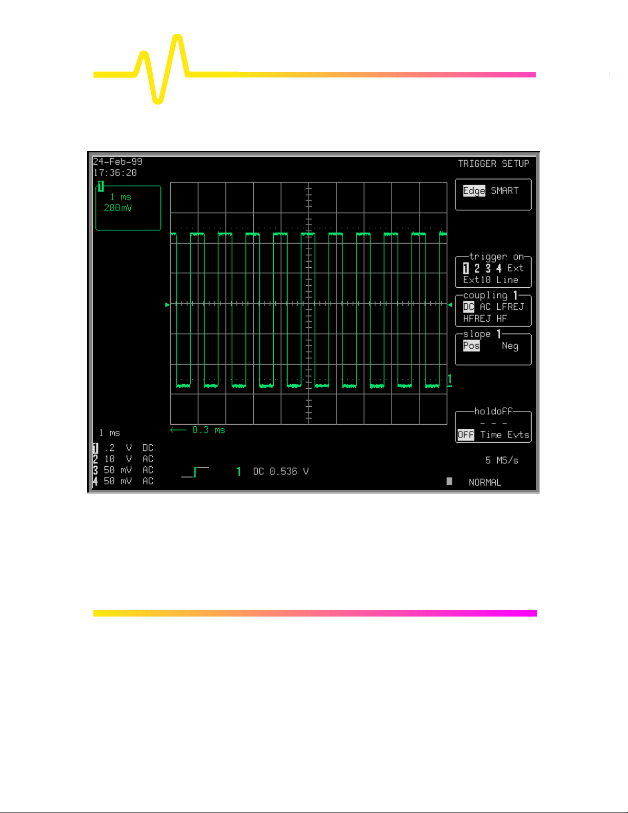
Modifying Trigger Settings Trigger adjustments are made directly using the front-panel controls
and with the trigger menus.
Rotating — for example — causes the scope to adjust the
trigger level of the highlighted trace.
Pressing accesses advanced trigger operations, such as
changing the glitch width or the hold-off timeout, which are
changed via the TRIGGER SETUP menu group (Fig. 8–1). Once
the trigger configuration has been modified, changes are stored
internally in a non-volatile memory.
This chapter describes
the triggering operations
and offers hints on how
to perform them. Along
with the standard menu
descriptions, schematics
show the trigger-menu
structure, and diagrams
explain how the main
triggers work.
TRIGGER SETUP
Edge
SMART
Figure 8–1. Main Trigger Menu.
8–1
Page 48

Triggers and When to Use Them
Edge or SMART
A variety of triggers for different applications can be
chosen from the two main trigger groups, the Edge and
SMART trigger types.
Edge Triggers In the Edge group of menus trigger conditions are defined by the
vertical trigger level, coupling, and slope. Edge triggers use simple
selection criteria to characterize a signal. They are most useful for
triggering on simple signals (see page 8–3).
SMART Trigger The SMART Trigger types allow additional qualifications to be
set before a trigger is generated. These qualifications can be
used to capture rare phenomena such as glitches or spikes,
specific logic states, or missing bits. A qualification might
include trigger generation only on a pulse wider or narrower than
a user-specified limit. Or it might require — to take but another
example — three trigger sources exceeding specific levels for a
minimum time.
Generally speaking, SMART Trigger offers various trigger
qualifications based on three basic abilities:
1. To count a specified number of events
2. To measure time intervals
3. To recognize a pattern input.
SMART explanations start on page 8–10 and on page menus 8–
29.
Trigger Symbols, illustrated throughout this chapter,
allow immediate on-screen recognition of the current
trigger conditions. There is a symbol for each Edge and
SMART Trigger type, with the more heavily-marked
transitions on the symbols indicating where a trigger will be
generated.
8–2
Page 49

Edge Trigger
Selecting Edge and its menus (Fig. 8–2) causes the scope
to trigger whenever the selected signal source meets the
trigger conditions. The trigger source is defined by the
trigger level, coupling, slope or hold-off.
Edge
Trigger on
Coupling
Slope Pos|Neg|Window
Holdoff
Figure 8–2. Edge Trigger Menu (see page 8–9).
1|2|3|4|Ext|Ext10|Line
DC|AC|LFREJ|HFREJ|HF
Off|Time (10 ns to 20 s)
|Events (1to 99 999 999)
8–3
Page 50

Triggers and When to Use Them
Trigger Source The trigger source may be:
Ø The acquisition channel signal (CH 1, CH 2 or CH 3, CH 4
on four-channel models) conditioned for the overall voltage
gain, coupling, and bandwidth.
Ø The line voltage that powers the oscilloscope (LINE). This
can be used to provide a stable display of signals
synchronous with the power line. Coupling and level are not
relevant for this selection.
Ø The signal applied to the EXT BNC connector (EXT). This
can be used to trigger the oscilloscope within a range of
± 0.5 V, or ± 5 V with EXT/10 as trigger source.
Level Level defines the source voltage at which the trigger circuit will
generate an event (a change in the input signal that satisfies the
trigger conditions). The selected trigger level is associated with
the chosen trigger source. Note that the trigger level is specified
in volts and is normally unchanged when the vertical gain or
offset is modified.
The Amplitude and Range of the trigger level are limited as
follows:
Ø ± 5 screen divisions with a channel as trigger source
Ø ± 0.5 V with EXT as trigger source
Ø ± 5 V with EXT/10 as trigger source
Ø None with LINE as trigger source (zero crossing is used).
Note: Once specified, Trigger Level and Coupling are
the only parameters that pass unchanged from mode
to mode for each trigger source.
Coupling This is the particular type of signal coupling at the input of the
trigger circuit. As with the trigger level, the coupling can be
independently selected for each source. Thus changing the
trigger source can change the coupling. The types of coupling
able to be selected are:
8–4
Page 51

Ø DC: All the signal's frequency components are coupled to
the trigger circuit. This is used in the case of high-frequency
bursts, or where the use of AC coupling would shift the
effective trigger level.
Ø AC: Here the signal is capacitively coupled. DC levels are
rejected and frequencies below 50 Hz attenuated.
Ø LF REJ: The signal is coupled via a capacitive high-pass
filter network. DC is rejected and signal frequencies below
50 kHz attenuated. This mode is used when stable triggering
on medium- to high-frequency signals is desired.
Ø HF REJ: Signals are DC-coupled to the trigger circuit and a
low-pass filter network attenuates frequencies above
50 kHz. The HF REJ trigger mode is used to trigger on low
frequencies.
Ø HF: Used for triggering on high-frequency repetitive signals
in excess of 300 MHz. Maximum trigger rates greater than
500 MHz are possible. HF triggering should be used only
when needed. It will be automatically overridden and set to
AC when incompatible with other trigger characteristics —
as is also the case for SMART Trigger. Only one slope is
available, indicated by the trigger symbol.
Slope Slope determines the direction of the trigger voltage transition
used for generating a particular trigger event. Like coupling, the
selected slope is associated with the chosen trigger source.
Hold-off Hold-off disables the trigger circuit for a given period of time or
a number of events after a trigger event occurs. It is used to
obtain a stable trigger for repetitive, composite waveforms. For
example, if the number or duration of sub-signals is known they
can be disabled by choosing an appropriate hold-off value.
Without Hold-off, the time between each successive trigger
event would be limited only by the input signal, the coupling, and
the oscilloscope's bandwidth. Sometimes a stable display of
complex repetitive waveforms can be achieved by placing a
condition on this time. This hold-off is expressed either as a time
or an event count, described on the following pages.
8–5
Page 52

Triggers and When to Use Them
Hold-off by Time This is the selection of a minimum time for triggers (Fig. 8–
3). A trigger is generated when the trigger condition is met
after the selected delay from the last trigger. The timing for
the delay is initialized and started on each trigger. The holdoff timeout should exceed the duration of the signal
displayed on screen. For instance, at a timebase setting of 1
ms/div, the time-out hold-off should at least exceed 10 ms.
Trigger Source: Positive Slope
Trigger
Event
Trigger can occur
Hold-off time Hold-off time
Generated Trigger
Trigger
Event
Trigger initiates
hold-off timer
Figure 8–3. Edge Trigger with Hold-off by Time.
Trigger
Event
Trigger initiates
hold-off timer
8–6
Page 53

Hold-off by Events Hold-off by events is initialized and started on each trigger
(Fig. 8–4 ). A trigger is generated when the trigger condition is met
after the selected number of events from the last trigger. Event here
refers to the number of times the trigger condition is met after the
last trigger. For example, if the number selected is two, the trigger
will occur on the third event.
Trigger Source: Positive Slope
Trigger
Event
Event
#1
Event
#2
Trigger
Event
Trigger can occur
Holdoff by 2 events Holdoff by 2 events
Generated Trigger
Trigger initiates
hold-off timer
Figure 8–4. Edge Trigger with Hold-off by Events.
Event
#1
Event
#2
Trigger initiates
hold-off timer
Trigger
Event
8–7
Page 54

Triggers and When to Use Them
Window Trigger
AVAILABLE ONLY WITH
9304C, 9310C, 9314C
SERIES
Trigger Level
On some scope models a “Window” Edge Trigger is also
available (Fig. 8–5). Two trigger levels are defined and a trigger
event occurs when the signal leaves the window region in either
direction.
Upper Region
WINDOW REGION
Lower Region
Time
Triggers
Figure 8–5. Edge Window Trigger.
8–8
Page 55

TRIGGER SETUP: Edge
Press to access menu selection of:
Ø Trigger source
Ø Coupling for each source
Ø Slope (positive or negative), and
Ø Hold-off by time or events.
Edge/SMART To select “Edge”
trigger on
For selecting the Edge trigger source (four-channel menu
shown).
coupling
To select the trigger coupling for the current source.
slope
To place the trigger point on either the “Pos ”-itive or “Neg”-ative slope of
the selected source. On those models featuring Window Trigger (9304C,
9310C, 9314C SERIES), this menu will also include a “Window” option,
which allows triggering whenever the input signal leaves a specified
voltage window, defined in the “window size” menu. The “window size”
menu becomes available on models featuring Window Trigger. It allows
adjustment of the window around a level defined using the Trigger
LEVEL knob.
holdoff
To allow the disabling of the oscilloscope's trigger circuit for a definable
period of time or number of events after a trigger event occurs. When
activated, “holdoff” can be defined as: a period of “Time”, or a number
of “Evts ” (an event being a change in the input signal that satisfies the
trigger conditions). The menu knob is used to vary the “holdoff” value.
Time hold-off values in the range 10 ns–20 s may be entered. Event
counts in the range 1–109 are allowed.
8–9
Page 56

Triggers and When to Use Them
SMART Trigger
SMART Trigger allows the setting of additional qualifications
before a trigger is generated. Depending on the oscilloscope
model, this can include triggers adapted for glitches, intervals,
abnormal signals, TV signals, state- or edge-qualified events,
dropouts and patterns.
Glitch Trigger Glitch Trigger (Fig. 8–6) is used to capture narrow pulses
inferior to or exceeding a given time limit. In addition, a width
range can be defined to capture any pulse that is comprised
within or outside the specified range — an Exclusion Trigger.
Glitch
Trigger on
Coupling
At end of Neg|Pos|Pulse
Width: l
than or equal
greater than
or equal to
Figure 8–6. Glitch Trigger Menu (see page 8–30).
ess
to
Width:
1|2|3|4|Ext|Ext10|Pattern
DC|AC|LFREJ|HFREJ|HF
Off|Time (2.5 ns to 20 s)
Off|Time (2.5 ns to 20 s)
8–10
Page 57

Applications In digital electronics circuits normally use an internal clock, and for
testing purposes a glitch can be defined as any pulse of width smaller
than the clock- or half-period. But generally speaking a glitch is a pulse
much faster than the waveform under observation. Glitch Trigger thus
has a broad range of applications in digital and analog electronic
development, ATE, EMI, telecommunications, and magnetic media
studies.
Pulse Smaller than
Selected Pulse Width
This Glitch Trigger selects a maximum pulse width (Fig. 8–7). It is
generated on the selected edge when the pulse width is less than the
selected width. The timing for the width is initialized and restarted on the
slope opposite to the edge selected. Widths of between 2.5 ns and 20 s
can be selected, but typically triggering will occur on glitches 1 ns wide.
Trigger Source
Glitch
Glitch width
width
Trigger can occur
Selected width
Generated Trigger
Figure 8–7. Glitch Trigger on pulse width < selected width.
8–11
Page 58

Triggers and When to Use Them
Exclusion Trigger Exclusion Trigger enables the exclusion of events over a
determined time interval. Exclusion Trigger is generated on the
selected edge when the pulse width is within or outside the
selected width range. For example (Fig. 8–8), only pulses
smaller than 25 ns or longer than 27.5 ns will generate the
trigger. The timing for the width is initialized and restarted on the
slope opposite to the edge selected. Widths of between 2.5 ns
and 20 s can be selected.
Figure 8–8. Exclusion Trigger. Only pulses within or outside the
boundaries of the width range are captured.
Applications Exclusion Triggers allow a signal’s normal width or period to be
specified, with the scope instructed to ignore the normally
shaped signals and trigger only on abnormal ones. Circuit
failures, for instance, can be looked for all the time.
8–12
Page 59

Interval Trigger Whereas Glitch Trigger performs over the width of a pulse,
Interval Trigger (Fig. 8–9) performs over the width of an
interval. An interval corresponds to the signal duration
separating two consecutive edges of the same polarity. Interval
Trigger is used to capture intervals that are inferior to or exceeding
a given time limit. In addition, a width range can be defined to
capture any interval that is comprised within or outside the specified
range — an Exclusion Trigger by Interval.
Interval
Trigger on
Coupling
Between
Interval: l
than or equal
greater than
or equal to
Figure 8–9. Interval Trigger Menu (see page 8–32).
ess
to
Interval:
1|2|3|4|Ext|Ext10|Pattern
DC|AC|LFREJ|HFREJ|HF
Pos|Neg
edges
Off|Time (10 ns to 20 s)
Off|Time (10 ns to 20 s)
Applications Interval Trigger is helpful for determining missing cycles or
transitions, and for ignoring unwanted signal reflections.
8–13
Page 60

Triggers and When to Use Them
Interval Smaller For this Interval Trigger, generated on a time interval smaller than
the one selected, a maximum interval between the two edges of the
same slope is chosen (Fig. 8–10). The trigger is generated on the
second edge if it occurs within the selected interval. The timing for
the interval is initialized and restarted whenever the selected edge
occurs. Intervals of between 10 ns and 20 s can be selected.
Trigger Source: Positive Slope
Interval width
Interval
width
Trigger can occur
Selected
interval
T
T
Generated Trigger
Figure 8–10. Interval Trigger: Trigger if the interval is smaller than the
selected interval.
8–14
Page 61

Interval Larger For this Interval Trigger, generated on an interval larger than the
one selected, a minimum interval between the two edges of the
same slope is chosen (Fig. 8–11). The trigger is generated on
the second edge if it occurs after the selected interval. The
timing for the interval is initialized and restarted whenever the
selected edge occurs. Intervals of between 10 ns and 20 s can
be selected.
Trigger Source: Positive Slope
Interval width
Interval
width
Trigger can occur
Selected
interval
T
T
Generated Trigger
Figure 8–11. Interval Trigger: Trigger if the interval is greater than
the selected width.
8–15
Page 62

Triggers and When to Use Them
Interval Between Range This Interval Trigger selects a maximum interval between the
two edges of the same slope (Fig. 8–12). The trigger is
generated on the second edge if it occurs within the selected
interval range. The timing for the interval is initialized and
restarted whenever the selected edge occurs. Intervals of
between 10 ns and 20 s can be selected.
Trigger Source: Positive Slope
Interval width
Interval
width
Trigger can occur
T1
Selected
ranges
T1
T2
T2
Generated Trigger
Figure 8–12. Interval Trigger: Trigger if the interval is between the
selected ranges.
8–16
Page 63

Interval Outside Range This Interval Trigger selects a minimum interval between the
two edges of the same slope (Fig. 8–13). The trigger is
generated on the second edge if it occurs after the selected
interval range. The timing for the interval is initialized and
restarted whenever the selected edge occurs. Intervals of
between 10 ns and 20 s can be selected.
Trigger Source: Positive Slope
Interval width
Interval
width
Trigger can occur
Selected
ranges
T1
T1
T2
T2
Generated Trigger
Figure 8–13. Interval Trigger: Trigger if the interval is outside the
selected ranges.
8–17
Page 64

Triggers and When to Use Them
Pattern Trigger Pattern Trigger (Fig. 8–14) enables triggering on a logical
NOT AVAILABLE ON
9304C, 9310C, 9314C SERIES
combination of the inputs CH 1, CH 2 (plus CH 3 and CH 4 on fourchannels models) and EXT. This combination, called a pattern, is
defined as the logical AND of trigger states. A trigger state is either
high or low: high when a trigger source is greater than the trigger
level (threshold); low when less than this threshold (Fig. 8–15). For
example, the pattern could be defined as present when the trigger
state for CH 1 is high, CH 2 is low, and EXT is irrelevant (X or don’t
care). If any of these conditions are not met, the pattern state is
considered absent. Limits can be selected from 10 ns to 20 s.
Pattern
Trigger on
Pattern
with
Coupling DC|AC|LFREJ|HFREJ
Level L|H|X|(Level value)
Holdoff
Figure 8–14. Pattern Trigger Menu (see page 8–33).
1|2|3|4|Ext (according to model)
Exiting|Entering
Off| Time (10 ns to 20 s)
|Evs (1 to 99 999 999)
8–18
Page 65

Applications Pattern Trigger is useful in digital design for the testing of complex
logic inputs or data transmission buses.
Threshold
CH 1
Threshold
CH 2
High
Low
High
Low
Pattern 1H*2L
Generated Trigger (Pattern Entering)
Generated Trigger (Pattern Exiting)
Figure 8–15. Pattern Trigger: Trigger when pattern conditions met.
8–19
Page 66

Triggers and When to Use Them
More About Pattern Trigger Once the pattern is defined, one of two transitions can be used to
generate the trigger. When the pattern begins, called entering the
pattern, a trigger can be generated. Alternatively, a trigger can be
generated when the pattern ends, exiting the pattern.
With pattern triggering, as in single source, either of these
qualifications can be selected: Hold-off for 10 ns up to 20 s, or
Hold-off for 1 to 99 999 999 events.
Set to Pattern Trigger, the oscilloscope always checks the logic
AND of the defined input logic states. However, with the help of
de Morgan's laws, the pattern becomes far more generalized.
Consider the important example of the Bi-level or Window Pattern
Trigger. Bi-level implies the expectation of a single-shot signal on
which the amplitude will go in either direction outside a known
range. To set up a Bi-level Pattern trigger, connect the signal to two
inputs: Channels 1 and 2 or any other pair that can be triggered on.
For example, the threshold of CH 1 could be set to +100 mV and
that of CH 2 at −200 mV. The Bi-level Trigger will occur if the
oscilloscope triggers on CH 1 for any pulse greater than +100 mV,
or on CH 2 for any pulse less than –200 mV. For improved
precision, the gains of the two channels should be at the same
setting.
In Boolean notation we can write:
Trigger CH 1 CH 2= + ,
i.e. trigger when entering the pattern CH 1 = high OR CH 2 = low.
By de Morgan's laws this is equivalent to:
Trigger CH 1 CH 2= ⋅ ,
i.e. trigger when exiting the pattern CH 1 = low AND CH 2 = high.
This configuration can be easily programmed.
The possibility of setting the threshold individually for each channel
extends this method so that it becomes a more general Window
Trigger: in order to trigger the input pulse amplitude must lie within
or outside a given arbitrary window.
Pattern Trigger has been designed to allow a choice of the trigger
point. By choosing 1L*2H entering, the trigger will occur at the
moment the pattern 1L*2H becomes true.
8–20
Page 67

Qualified Triggers In the case of Qualified Triggers (Fig. 8–16), a signal’s transition
above or below a given level, the validation, serves as an
enabling, or qualifying, condition for a second signal that is the
source of the trigger.
Two Qualified Triggers are available: State-Qualified, where the
amplitude of the first signal must remain in the desired state
until the trigger occurs, and Edge-Qualified, for which the
validation is sufficient and no additional requirement is placed
on the first signal.
A Qualified Trigger can occur immediately after the validation or
within a set time after it. Or it can occur following a
predetermined time delay or number of potential trigger events.
The time delay or trigger count is restarted with every validation.
Qualified
Qualified
By
Trigger on
Only after 1|2|3|4|Ext|Ext10|Pattern
Goes and
stays
Wait
Edge|State qualifier
1|2|3|4|Ext|Ext10
Above|Below|Value
Off|Time <| Time> (10 ns to
20 s)| Evs (1 to 99 999 999)
By
Trigger on
After 1|2|3|4|Ext|Ext10|Pattern
Has gone Above|Below|Value
Wait
Edge|State qualifier
1|2|3|4|Ext|Ext10
Off|Time <| Time> (10 ns to
20 s)| Evs (1 to 99 999 999)
Figure 8–16. State- and Edge-Qualified Trigger Menus (see pages 8–35 and 8–36).
8–21
Page 68

Triggers and When to Use Them
Qualified Triggers offer the choice of generating a trigger either
when the selected pattern is present or absent. As with Pattern
Trigger, the pattern is defined as a logical AND combination of
trigger states that are either high or low: high when a trigger source
is greater than the selected trigger level, and low when it is less
than. For example, a pattern might be defined as present when the
trigger states for Channels 1 and 2 are high and EXT is low. If any of
these conditions is not met, the pattern state is considered absent.
Qualified Triggers allow an additional qualification once the selected
pattern state occurs. For example: “wait for 10 ns up to 20 s, trigger
on CH 1 to the 99 999 999th event”. The pattern is used to qualify
the trigger without actually generating it. Triggering will occur when
another signal, the trigger source, meets its trigger condition while
the pattern is present. The trigger source itself is not allowed in the
pattern.
Applications Typical applications can be found wherever time violations
occur, such as in micro-processor debugging or
telecommunications.
State-Qualified with Wait State-Qualified Trigger with Wait (Fig. 8–17) is determined by
the parameters of Time and number of Events:
Ø Time selects a delay from the start of the desired pattern.
After the delay (timeout) and while the pattern is present, a
trigger can occur. The timing for the delay is restarted when
the selected pattern begins
Ø Events selects a minimum number of events of the trigger
source. An event is generated when a trigger source meets
its trigger conditions. On the selected event of the trigger
source and while the pattern is present, a trigger can occur.
The count is initialized and started whenever the selected
pattern begins, and continues while the pattern remains.
When the selected count is reached, the trigger occurs.
8–22
Page 69

Trigger Source: Positive Slope
Qualifier: Pattern Present
Trigger can occur
Generated Trigger
Figure 8–17. State-Qualified by Wait: Trigger after timeout.
Selected wait
As Figure 8–17 illustrates, a trigger is generated on a rising edge
whenever the pattern is asserted (pattern present) and the wait
timeout has expired. The timeout is, respectively, activated or
disabled once the pattern is asserted or absent.
8–23
Page 70

Triggers and When to Use Them
Edge-Qualified with Wait Like its State-Qualified equivalent, Edge-Qualified with Wait
(Fig. 8–18) is conditioned by Time and Events:
Ø Time Selects a delay from the start of the desired pattern.
After the delay (timeout) and before the end of the pattern, a
trigger can occur. The timing for the delay is restarted when
the selected pattern begins.
Ø Events selects a minimum number of events of the trigger
source. An event is generated when a trigger source meets
its trigger conditions. On the selected event of the trigger
source and before the end of the pattern, a trigger can
occur. The count is initialized and started whenever the
selected pattern begins. It continues while the pattern
remains. When the selected count is reached, the trigger
occurs.
Trigger Source: Positive Slope
Qualifier: Pattern Present
Trigger can occur
Selected time
T
Generated Trigger
Figure 8–18. Edge-Qualified by Wait: Trigger after timeout.
8–24
T
Page 71

TV Trigger A special kind of Edge-Qualified Trigger, TV Trigger allows
stable triggering on standard or user-defined composite video
signals, on a specific line of a given field. Applications can be
found wherever TV signals are present. And TV Trigger can be
used on PAL, SECAM or NTSC systems.
A composite video signal on the trigger input is analyzed to
provide a signal for the beginning of the chosen field — “any”,
“odd” or “even” — and for a signal at the beginning of each line.
The field signal provides the starting transition, and the
beginnings of line pulses are counted to allow the final trigger on
the chosen line.
Each field, the number of fields, the field rate, interlace factor,
and number of lines per picture must be specified — although
there are standard settings for the most common types of TV
signals. TV Trigger can also function in a simple any-line mode.
TV
TV signal on
# of fields
TV type Standard | Custom
Trigger on Line | Field
1|2|3|4|Ext|Ext 10
1|2|4|8
as: 625/50/2:1| 525/60/2:1
(Standard)
as: Line| Hz | Interlacing
1 to 1500| 50/60 | 1:1/2:1/
4:1/8:1/
(Custom)
Figure 8–19. TV Trigger Menus (see page 8–34 )
8–25
Page 72

Triggers and When to Use Them
Notes for TV Trigger
Ø Because most TV systems have more than two fields, the enhanced field-counting
capability (FIELDLOCK) allows the oscilloscope to trigger consistently on a chosen
line within a chosen field of the signal. The field-numbering system is relative, in that
the oscilloscope cannot distinguish between lines 1, 3, 5, and 7 (or 2, 4, 6, and 8) in an
absolute way.
Ø For each of the characteristics the following remarks apply:
Ø 625/50/2:1 (PAL and SECAM systems)
This setting should be used for most of the standard 50-field signals. The lines
may be selected in the range 1 to 626 where line 626 is identical to line 1.
Number of fields: eight is most useful for color PAL signals; four for SECAM
signals.
Ø 525/60/2:1 (NTSC systems)
This setting should be used for standard 60-field NTSC signals. The lines can
be selected in the range 1 to 1051, where line 1051 is identical to line 1.
Number of fields: four is most useful for US-type NTSC systems.
Ø ?/50/?, ?/60/?
In order to allow maximum flexibility, no line-counting convention is used. The
line count should be thought of as a line-synchronizing pulse count. It
includes the transitions of the equalizing pulses. For certain extreme cases,
the field transition recognition will no longer work, and only the “any line”
mode will be available.
Ø The enhanced field-counting capability cannot be used for RIS acquisitions.
Ø Composite video signals must have negative-going synch to be decoded correctly.
8–26
Page 73

Dropout Trigger Dropout Trigger (Fig. 8–20) provides triggering whenever the
signal disappears for a selectable period of time. The trigger is
generated at the end of the time-out period following the “last”
trigger source transition. Time-outs of between 25 ns and 20 s
can be selected.
Dropout
Trigger after
timeout if no edge
occurs on
1|2|3|4|Ext|Ext10
With
slope
Within Time (25 ns to 20 s)
Figure 8–20. Dropout Trigger Menu (see page 8– 37)
Positive|Negative
Applications Dropout Trigger is useful for detecting interruptions in data
streams such as network hang-ups and microprocessor crashes.
A typical application is on the last ‘normal’ interval of a signal
that has disappeared completely. This is essentially a singleshot application, usually with a pre-trigger delay. RIS acquisition
is not useful here because the timing of the trigger timeout is
insufficiently correlated with the input channel signals.
8–27
Page 74

Trigger Source
Trigger can occur
Generated Trigger
Triggers and When to Use Them
Wait timeout
Figure 8–21. Dropout Trigger: A trigger occurs when the timeout has expired.
8–28
Page 75

TRIGGER SETUP: SMART
Press to access, too, the various SMART Trigger
types, to trigger on:
Ø Glitches
Ø Intervals
Ø Abnormal signals (Exclusion Trigger)
Ø Patterns (NOT AVAILABLE ON 9304C, 9310C, 9314C SERIES)
Ø State- or edge-qualified events
Ø TV signals
Ø Dropouts.
Edge/SMART To select “SMART
SETUP SMART TRIGGER
This is primary menu that accesses the “SMART TRIGGER”
menu group, for choosing the type of SMART Trigger required
from the “type” secondary menu. This and the other SMART
menus are described starting page 8–30.
8–29
Page 76

SMART TRIGGER — Glitch
type
trigger on
coupling
at end of
Triggers and When to Use Them
To select “Glitch”.
For selecting the trigger source (four-channel menu shown).
To select the trigger coupling.
To define the test on either “Pos”-itive or “Neg”-ative pulses.
width ≤
When “On” instructs the instrument to trigger if the pulse is smaller
than the value defined in this field. The value can be adjusted with
the associated menu knob, while the test can be turned on or off by
pressing the menu button, and used in combination with the
“width ≥” test. Width values in the range 2.5 ns to 20 s can be
entered.
& width ≥
“On” instructs the instrument to trigger if the pulse is greater than
the value defined in that field. The value can be adjusted using the
associated menu knob, and the test turned on or off with the menu
button in combination with the “width ≤” test menu selection. The
two width limits are combined to select glitches within (“&”) a certain
range if the “width ≤” value is greater than the “width ≥” value.
Otherwise, they are combined to select glitches outside this range.
8–30
Page 77

SMART TRIGGER — Glitch — Pattern (NOT ON 9304C, 9310C, 9314C SERIES)
When “Pattern” is selected in Glitch mode, the instrument triggers
on the logic AND of up to five sources.
type
To select “Glitch”.
trigger on
To select “Pattern” (four-channel menu shown).
for pattern
For selecting pattern “Present” or “Absent”.
width ≤
To trigger if the pattern is present or absent for less than the time
value defined in that field. The value can be adjusted with the
associated menu knob and the test commuted to “≥” by pressing the
corresponding menu button.
& width ≥
To trigger if the pattern is present or absent for more than the time
value defined in that field. The value can be adjusted and the test
commuted to “≤ ” as per “width ≤ ”.
8–31
Page 78

SMART TRIGGER — Interval
type
To select “Interval”.
trigger on
For selecting the trigger source (four-channel menu shown).
coupling
For selecting the trigger coupling.
between
To define the interval between two adjacent “Pos”-itive or “Neg”
-ative edges.
Triggers and When to Use Them
interval ≤
To trigger if the interval is smaller than the value defined here,
which can be adjusted using the associated knob. The test can be
turned on or off with the corresponding menu button, and can be
used in combination with the “interval ≥” test. Interval values in the
range 10 ns to 20 s may be entered.
OR interval ≥
To trigger if the interval is greater than the value defined here,
which can be adjusted using the associated menu knob The test can
be turned on or off using the corresponding menu button, and can
be used in combination with the “interval ≤” test. The two interval
limits are combined to select intervals within (“&”) a range if the
“interval ≤” value is greater than the “interval ≥” value. Otherwise
they are combined to select intervals outside (“OR”) the range.
8–32
Page 79

SMART TRIGGER — Pattern (NOT ON 9304C, 9310C, 9314C SERIES)
type
To select “Pattern”.
trigger on
To select “Entering” for the scope to trigger when the pattern starts
being true, and “Exiting” for triggering when it stops being true .
Pattern with
For selecting the channel to be modified using the lower menus’
corresponding menu buttons (four-channel menu shown).
coupling
To select the desired coupling. HF coupling is not available for
Pattern Trigger.
level
For modifying these values using the associated knob — adjusts the
level — and the corresponding menu button, which chooses
“L” (low), “H” (high), or “X” (Don't care).
holdoff
To disable the trigger circuit for a definable period of time or number
of events after a trigger event (a change in the input signal that
satisfies the trigger conditions). When not turned off, holdoff can be
defined as a period of “Time” or a number of “Evts” (events). Use
the associated menu knob to vary the “holdoff” value. Time holdoff
values in the range 10 ns–20 s may be entered. Event counts in the
range 1–109 are allowed.
8–33
Page 80

SMART TRIGGER — TV
Triggers and When to Use Them
type
To select “TV” .
TV signal on
For selecting the trigger source (four-channel menu shown).
# of fields
To define the number of fields — up to eight.
TV type
For selecting either “Standard” or “Custom” TV decoding.
as
When “Standard” is chosen, for selecting either “625/50/2:1” (PAL
SECAM) or “525/60/2:1” (NTSC) standards.
When “Custom” is selected, for specifying the number of lines and
cycles, and setting the interlacing factor for non-standard TV
signals.
trigger on
For selecting the line and field number on which to trigger.
8–34
Page 81

SMART TRIGGER — Qualified — State
type
To select “Qualified”.
by
To select “State”.
trigger on
For selecting the trigger source — the other conditions for this
source can be set up using Edge Trigger (four-channel menu
shown).
only after
To select the qualifier source — the other conditions can be set up
using Edge Trigger.
goes & stays
For selecting the qualifier threshold using the associated knob, and
using the menu button to select whether the qualifier signal will be
valid either “Above” or “Below” that threshold.
When “Pattern” is selected as the qualifier source, this menu is
used to determine whether the pattern should be present or absent.
wait/within
To specify the time limit (“T<”) for accepting the trigger event. And
alternatively, to specify how much time (“T>”) or how many trigger
events (“Evs”) should be allowed before the acquisition is taken on
the next trigger event. The qualifier signal must remain valid until
the final trigger has been received. The time value can be chosen in
the range 10 ns–20 s. The trigger event count can be chosen in the
range 1–109.
8–35
Page 82

Triggers and When to Use Them
SMART TRIGGER — Qualified — Edge
type
To select “Qualified”.
by
To select “Edge”.
trigger on
For selecting the trigger source — the other conditions for this
source are set up using Edge Trigger (four-channel menu shown).
after
For selecting the qualifier source — other setup conditions use Edge
Trigger (four-channel menu shown).
has gone
To adjust the qualifier threshold and determine whether the qualifier
signal is valid once it “has gone” above or below that threshold.
“Pattern” selected as the qualifier source determines whether the
pattern should be present or absent.
wait/within
To specify the time limit (“T<”) for accepting the trigger event. Or, to
specify the delay in time (“T>”) or number of trigger events (“Evs”)
after a valid transition has occurred. A trigger can only be accepted
after this delay. Any subsequent qualifier event restarts this count.
The time value can be chosen in the range 10 ns–20 s. The trigger
event count can be chosen in the range 1–109.
8–36
Page 83

SMART TRIGGER — Dropout
type
To select “Dropout”.
trigger after timeout, if NO edge occurs on
For selecting the trigger source (four-channel menu shown).
with slope
To define whether the measurement starts on a “Positive” or
“Negative” slope of the trigger signal.
Within… of previous edge
For defining the time-out value in the range 25 ns–20 s.
8–37
Page 84

9
ZOOM + MATH Controls
A wide range of Zoom and Mathematical processing
functions (detailed in the next chapter) can be performed
on acquired waveforms with the controls described here.
Four processed traces are
available for straight-forward
zooming or for waveform
mathematics. Any one of
these traces, A, B, C or D,
can be set up to zoom a
trace acquired on any
channel or stored in any of
the four reference memories
M1–4. Or zoom any of the
other three original traces.
Thus Trace A, for example,
could be set up to zoom
Trace B, C, or D, but not
itself. The Displayed Trace
label at left of screen
indicates the source.
ZOOM + MATH
The
corresponding trace A, B, C or D. When a trace is switched on, the
POSITION and ZOOM knobs and the RESET button will then be
attributed to this, the active trace.
The SELECT ABCD button assigns the controls to the
active trace for adjustment, as only one trace can be modified at
a time. Pressing this button activates the next trace, in A–D
sequence.
The four ZOOM + MATH knobs adjust the horizontal and
vertical positions and expansion factors of the zoomed trace…
9–1
TRACE ON/OFF buttons display the
Page 85

ZOOM + MATH
The POSITION knob repositions zoomed traces
horizontally. If the source of the expanded waveform is
displayed, an intensified region corresponding to the area of
expansion is shown.
Whereas the vertically repositions the active trace.
The ZOOM knob horizontally expands or contracts the
active trace. If the source of the zoomed trace is also displayed,
it will show an intensified region corresponding to the area of
expansion.
While the vertically expands or contracts the active
trace.
The RESET button resets the vertical and horizontal
POSITION and ZOOM.
Finally, the menu-entry button accesses the zoom, math
and sequence segment features. See next chapter for details.
9–2
Page 86

10
Zoom, Mathematics and Math Setup
Zooming for Precise Waveform
Measurements
Several traces can be zoomed from a single waveform to
obtain precise timing measurements.
For instance, on a waveform composed of two pulses separated
by a long delay, Trace A could be made a zoom of the first
pulse, and Trace B a zoom of the second.
The combination of long memory and zooming allows extremely
accurate time interval measurements. And the time resolution
on the viewed trace can be significantly improved.
For example, choosing 50 000 points per channel on a timebase
of 0.1 ms/div, traces can be expanded to as much as 50 ns/div
— a factor of 2000. Using Relative Time cursors (see Chapter
14), a delay of, say, 500 µs could be measured with resolution
as high as 0.5 ns. Even with as many as eight million points
acquired, zooming can be done until there are only a few points
on the screen.
Using Multi-Zoom With Multi-Zoom, the zoomed region of the waveform can be
moved simultaneously along two or more different traces, or two
or more regions of the same trace.
When “Multi-Zoom” “On” is selected from the “ZOOM – MATH”
menu (see page 10–8), the horizontal zoom and position
controls apply simultaneously to all displayed traces — A, B, C
and D — allowing similar sections of different traces to be
viewed at the same time. The vertical controls still act
individually on the traces: switching from one trace to another is
done using the TRACE ON/OFF buttons. The highlighting of
trace titles in the Displayed Trace label indicates an active MultiZoom.
Zooming Math Functions When Trace A, B, C or D is defined as a mathematical function
rather than as a simple zoom (see next section), the zoom controls
remain operative and defining another trace as a zoom of the math
function becomes unnecessary. In order to view the entire
10–1
Page 87

Zoom, Mathematics and Math Setup
mathematical function, simply cancel any expansion or position
change by pressing RESET.
10–2
Page 88

Math Functions and Options
Coverage of the Setup
menus for configuring
zoom, math and
waveform processing
functions starts page
10–6. Averaging and
Extrema are outlined on
this and the following
pages.
For details on Enhanced
Resolution filtering, see
Appendix B.
How to Set Up for FFT
(Fast Fourier Transform)
is explained at the
conclusion of this
chapter, while a
complete description of
FFT practice and theory
is presented in Appendix
C.
Information on each of
the Waveform
Processing packages on
option is to found in
A wide range of standard or optional mathematical and
waveform processing functions are available.
The scope’s standard waveform mathematics functions consist
of waveform negation, identity, addition, subtraction,
multiplication and division, summed averaging of up to 1000
waveforms and the (sin x)/x interpolation function.
Advanced waveform processing features, depending on the
options installed, include:
Ø Continuous Averaging (menus page 10–11);
Ø Summed Averaging of up to 1 000 000 waveforms (menus
10–11);
Ø Enhanced Resolution by up to 3 bits with filtering (menus
10–12);
Ø Extrema — envelope of many waveforms (menus 10–13);
Ø Fast Fourier Transform, including FFT averaging (menus
10–14 and 10–15);
Ø Mathematical Functions such as Integral, Derivative,
Logarithm, Exponential, Square, and Square Root (menus
10–16);
Ø Parameter Analysis, histogramming, trending and statistical
analysis (menus page 10–17).
Continuous Averaging This is the repeated addition, with unequal weight, of successive
source waveforms. It is particularly useful for reducing noise on
signals that drift very slowly in time or amplitude.
However, the statistics of a continuous average tend to be worse
than those from a summed average (see next page) on the
same number of sweeps. This is because the most recently
acquired waveform has more weight than all previously acquired
ones: the continuous average is dominated by the statistical
fluctuations of the most recently acquired.
10–3
Page 89

Zoom, Mathematics and Math Setup
The weight of ‘old’ waveforms in the continuous average
gradually tends to zero (following an exponential rule) at a rate
that decreases as the weight increases.
Summed Averaging Summed Averaging is the repeated addition, with equal weight,
of successive source waveform records. If a stable trigger is
available, the resulting average has a random noise component
lower than that of a single-shot record.
Whenever the maximum number of sweeps is reached, the
averaging process stops. An even larger number can be
accumulated simply by changing the number in the “SETUP”
“for” menu. However, the other parameters must be left
unchanged or a new averaging calculation will be started.
The process may be interrupted by changing the trigger mode
from NORM to STOP or by turning off the active trace using the
respective buttons. Averaging will be resumed when the inverse
is done. The accumulated average is reset by pushing the
CLEAR SWEEPS button or changing an acquisition parameter
such as input gain, offset, coupling, trigger condition, timebase
or bandwidth limit. The number of current averaged waveforms
of the function or its expansion is shown in the Displayed Trace
label.
When summed averaging is selected, the display is updated at a
reduced rate — about once every 1.5 s — in order to increase
the averaging speed (points and events per second).
Summed averaging can also be done on sequence waveforms
to give the average of the segments. And it can be applied to an
expansion of a sequence segment, giving the segment’s
average waveform over many sequence acquisitions.
Extrema Waveforms These are computed by a repeated comparison of successive
source waveform records with the already-accumulated extrema
waveform, which consists of a maxima (roof) and a minima
(floor) record. Whenever a given data point of the new
waveform is greater than the corresponding maximum roofrecord value, or less than the corresponding floor value, it
replaces it. Thus the maximum and the minimum envelope of all
waveform records is accumulated.
Roof and Floor records can be displayed individually or together.
10–4
Page 90

Whenever the selected maximum number of sweeps is reached,
the accumulation stops. The same process may be interrupted
by changing the trigger mode from Normal to Stopped or by
turning off the function trace. Accumulation will continue when
these actions are reversed.
The currently accumulated extrema waveform may be reset by
either pushing the CLEAR SWEEPS button or by changing an
acquisition parameter such as input gain, offset, coupling, trigger
condition, or the timebase- or bandwidth-limit. The number of
currently accumulated waveforms is displayed in the function’s
Displayed Trace Label of that of its zoom expansion.
Whenever the maximum number of sweeps is reached, an even
larger number can be accumulated simply by changing the
number in the “SETUP” “for” menu. However, the other
parameters must be left unchanged or the extrema calculation
will be restarted.
10–5
Page 91

Zoom, Mathematics and Math Setup
Using Waveform Mathematics
Waveform mathematics can be applied to any channel or
reference memory. And any trace of A, B, C or D can be set
up as a math function, allowing several computations to be
made in sequence.
For example: Trace A could be set up as the difference between
Channels 1 and 2; Trace B defined as the average of A, and
Trace C made the integral of B — thus displaying the integral of
the averaged difference between Channels 1 and 2.
In order to avoid slowing down the instrument with unwanted
computations, a particular mathematical function is only
computed when its display is turned on. However, using the
same example as above, it would be sufficient to display Trace
C alone, as the instrument knows it must compute A and B as
intermediate steps to C.
Waveform processing can also take time when many data
points are involved. This delay can be cut by limiting the number
of data points used in the computation. To do this, the
instrument will process the entire waveform by taking every Nth
point, where N depends on the timebase and the desired
maximum number of points, and the first point taken is always
the data value at the left-hand edge of the screen.
Combining Channels Zoom and math functions on Traces A, B, C, D and Reference
Memories M1, M2, M3, M4 use the instrument’s system memory,
which is dynamically allocated to each trace as required. When
more acquisition memory is achieved by combining channels, a
single long trace can consume all the reference memory or zoom
and math trace capacity in the instrument. When this happens, an
on-screen warning message will avert accidental storing of a new
trace to a reference memory already in use.
Note: A processing title for each displayed trace will be
shown in the Displayed Trace Label. If the title is missing,
the desired processing cannot be done and the contents
of the trace remain unchanged.
10–6
Page 92

Page 93

Zoom, Mathematics and Math Setup
Configuring for Zoom and Math
Press
traces and execute any zoom, math function using the “ZOOM
+ MATH” menus.
Any trace and function can be chained to another trace and function (not
all functions shown are necessarily available). Trace A, for example,
could be configured to average Channel 1, Trace B could be made a
Fourier Transform (FFT) of A, and Trace C a zoom of B. All traces can
be viewed simultaneously on-screen using the ZOOM + MATH TRACE
ON/OFF buttons. Any function can be zoomed directly.
REDEFINE A, B, C, or D
To select the trace to be redefined and accesses the “SETUP”
menus (described in the remainder of this chapter, using A as an
example).
Multi-Zoom
For switching Multi-Zoom “On” or “Off”. When “On”, all displayed
traces (A,B,C,D) are simultaneously controlled by the horizontal
POSITION and ZOOM knobs. When “OFF”, only the active trace,
chosen using the SELECT ABCD button, is controlled by
POSITION and ZOOM.
to enable the configuration of any of the four
Selected (NOT SHOWN)
When a trace with a zoom of a sequence-mode waveform is
selected, the “Selected” menu — not shown here — becomes
accessible. Pressing the corresponding menu button toggles the
selection between display of a single, specific “Segment” and “All
Segments”. With the former selected, the associated knob can be
used to step through the segments and choose one.
for Math use max points…
For selecting the maximum number of points for all math operations
— a low number increases computation speed.
10–8
Page 94

Zoom
Zoom and Math Setup Menus
use Math?
For toggling between “No” (Zoom only) and “Yes” (Math functions)
SETUP.
Trace A, B, C or D is ZOOM of
To select the source trace to be zoomed (four-channel menu
shown).
10–9
Page 95

Zoom, Mathematics and Math Setup
Arithmetic — allows addition, subtraction, multiplication and division, as well as
choice of the two operands and the operator. The example on this
page shows a setup of trace A as the sum of Channels 1 and 2.
use Math?
To choose a math function.
Math Type
To select “Arithmetic”.
Sum
Difference
Product
Ratio
For selecting the operator.
1 2 3 4 B C D
M1 M2 M3 M4
To select one of two operand source traces (four-channel menu
shown).
plus 1 2 3 4 B C D
M1 M2 M3 M4
To select the other operand source trace (four-channel menu
shown).
10–10
Page 96

Zoom and Math Setup Menus
Average — offers Summed (Linear) or Continuous (Exponential) Averaging.
Shown here is an example setup of trace A as a Summed Average
(over 1000 sweeps) of Channel 1. See also page 10–3.
use Math?
To choose a math function.
Math Type
To select, in this case, “Average” (other choices in the example
menu shown here include options not available on the standard
scope).
Avg Type
To select “Summed” or “Continuous Average ”.
for / weight
When “Summed” is selected, this menu (“for”) is used to define the
number of sweeps. When “Continuous Average” is chosen, the
same menu becomes “weight” and is used to define the weight,
similar to number of sweeps.
In “for” the first n sweeps will be taken into account, whereas in
“weight” the last sweep will be given a weight of 1 and the previous
result a weight of n in calculating the new average.
of
For selecting the source trace for averaging (four-channel menu
shown).
10–11
Page 97

Zoom, Mathematics and Math Setup
Enhanced Resolution
*
— allows the selection of low-pass digital filters that increase the
resolution of the displayed signal at the expense of its bandwidth.
Appendix B gives a detailed explanation.
These digital filters work very much like analog bandwidth-limit
ones. In Single-Shot mode, they and the sampling speed affect
bandwidth. If high bandwidth is needed at slow timebases,
averaging and repetitive sampling should be considered.
use Math?
To choose a math function.
Math Type
To select “Enhanced Resolution”.
enhance by
For selecting the filter that will enhance resolution of the displayed
signal from one to three bits in 0.5-bit steps.
1 2 3 4 B C D
M1 M2 M3 M4
To select the source trace for filtering (four-channel menu shown).
*
Only with WP01 Advanced Math package. See “Signal
Analysis” in Appendix A for specifications.
10–12
Page 98

Zoom and Math Setup Menus
SETUP Extrema
†
— used for acquiring a trace envelope over many acquisitions (see
also page 10–4).
use Math?
To choose a math function.
Math Type
To select “Extrema”.
limits
To select either “Envelope”, “Floor” or “Roof ”. Floor shows only the
lower, and Roof only the upper part of the envelope. Changing the
limits does not force the analysis to start again.
for
For selecting the number of sweeps.
of
To select the source trace (four-channel menu shown).
†
Only with WP01 Math package. See “Signal Analysis” in
Appendix A for specifications.
10–13
Page 99

Zoom, Mathematics and Math Setup
SETUP — FFT
‡
— used to display the Fast Fourier Transform (FFT) of a signal and
visualize it in the frequency domain. See the final section of this
chapter, and Appendix C, for when and how to use FFT.
use Math?
To choose a math function.
Math Type
For selecting “FFT”.
FFT result
To select the FFT’s output format: “Imaginary”, “Magnitude”,
“Phase”, “Power Dens”-ity, “Power Spect”-rum, “Real ” or “Real +
Imag”.
with window
Using the corresponding menu button to select the FFT window type
from “Rectangular”, “Hanning”, “Hamming ”, “Blackman-Harris”,
and “Flat-top”. And the associated knob to select “AC” or “DC ”.
of
For selecting the source trace (four-channel menu shown).
Note: During Fast Fourier Transform computation the FFT
sign is displayed in the lower right-hand corner of the
screen. The computation of FFT on long time-domain
records can take time. The computation can be interrupted
or aborted at any time using any front-panel control.
‡
Only with WP02 Spectral Analysis package. See “Signal
Analysis” in Appendix A for specifications.
10–14
Page 100

Zoom and Math Setup Menus
SETUP — FFT Average§— used for displaying the FFT power averaging of an FFT source
trace, power averaging being useful for characterizing broadband
noise or periodic signals without a stable trigger signal. Total power
— signal and noise — is measured at each frequency. The source
trace must be an FFT function. See the final section of this chapter,
and Appendix C, for when and how to use FFT.
use Math?
To choose a math function.
Math Type
To select “FFT AVG”.
FFT result
To select the output format of the FFT Average: “Magnitude”,
“Power Density”, “Power Spectrum”.
for
For selecting the number of sweeps.
of
To select the FFT source.
Note: FFT Average can be reset by pressing CLEAR
SWEEPS. The number of currently accumulated
waveforms is then shown in the Displayed Trace field of
the function or its expansion.
§
Only with WP02 Spectral Analysis package. See “Signal
Analysis” in Appendix A for specifications.
10–15
 Loading...