

Page 1

Landscape Management System
User’s Manual
LMS v. 1.7 – November, 1999
Compiled and Edited by:
Christopher E. Nelson
Contributions by:
Christopher E. Nelson
James B. McCarter
Jeremy Wilson
Patrick J. Baker
Justin S. Hall
Principal Investigator:
Chadwick D. Oliver
June 2, 1999
Page 2

Table of Contents
Table of Contents............................................................................................................................................................i
Manual Organization...................................................................................................................................................vi
Introduction.....................................................................................................................................................................1
What is the Landscape Management Project?........................................................................................................1
Description of the Landscape Management System..............................................................................................1
LMS System Requirements.......................................................................................................................................2
Typographic Conventions..........................................................................................................................................2
Acknowledgements.....................................................................................................................................................3
Software License .........................................................................................................................................................5
Getting More Information..........................................................................................................................................5
Contact Information....................................................................................................................................................5
Obtaining and Installing LMS....................................................................................................................................7
Obtaining a copy of the Landscape Management System ....................................................................................7
Installing the Landscape Management System......................................................................................................7
Windows 95/98/NT.................................................................................................................................................7
Windows 3.x............................................................................................................................................................7
Basic Functions...............................................................................................................................................................8
What is a Landscape Management System Portfolio?......................................................................................8
General Functions.......................................................................................................................................................8
Opening a Portfolio…............................................................................................................................................8
Saving a Portfolio…...............................................................................................................................................9
Closing a Portfolio..................................................................................................................................................9
Restoring a Portfolio...............................................................................................................................................9
Backing up a Portfolio..........................................................................................................................................10
Viewing the Portfolio Log…..............................................................................................................................10
Flushing the Cache…...........................................................................................................................................11
Projecting Stands and Landscapes .........................................................................................................................11
Projecting Stands…..............................................................................................................................................11
Projecting Landscapes…. ....................................................................................................................................12
Changing the Current Year….............................................................................................................................12
Treating Stands and Landscapes.............................................................................................................................13
Treatment Dialog Box… ...................................................................................................................................... 13
Select Stand.........................................................................................................................................................14
Select Thinning....................................................................................................................................................14
Stand Subset Selection ........................................................................................................................................14
Ingrowth ..............................................................................................................................................................15
Apply To..............................................................................................................................................................15
Specific Examples of Treating Stands..............................................................................................................16
Thinning a Stand .................................................................................................................................................16
Vegetation Control..............................................................................................................................................16
Regenerating a Stand...........................................................................................................................................17
Simulating Ingrowth and Regeneration...............................................................................................................18
Analyzing Stands and Landscapes.........................................................................................................................19
Tables......................................................................................................................................................................19
Table Dialog Box…….........................................................................................................................................19
Sending a Table to a Spreadsheet........................................................................................................................21
Charts......................................................................................................................................................................21
Chart Dialog Box…….........................................................................................................................................21
Displaying a Chart...............................................................................................................................................22
i
Page 3

Closing Charts…….............................................................................................................................................23
Visualizations ........................................................................................................................................................ 23
Stand Visualization……......................................................................................................................................24
Stand Comparison Visualization…….................................................................................................................26
Landscape Visualization……..............................................................................................................................28
Using Scenarios Files................................................................................................................................................29
Scenario File Format............................................................................................................................................30
Scenario File Keywords.......................................................................................................................................30
Scenario Editor...........................................................................................................................................................31
Scenario Editor Dialog Box…............................................................................................................................32
Scenario File Information....................................................................................................................................32
Year and Stand Selection ....................................................................................................................................32
Treatment Selection.............................................................................................................................................33
Control Buttons ...................................................................................................................................................33
Treatment Specification Section .........................................................................................................................34
Using the Scenario Editor....................................................................................................................................34
Adding a Treatment.............................................................................................................................................34
Removing a Treatment........................................................................................................................................36
Replacing a Treatment.........................................................................................................................................37
Portfolio Editor...........................................................................................................................................................38
Portfolio Editor Window ..................................................................................................................................... 39
Changing the Projection Step Size.....................................................................................................................39
Copying a Portfolio...............................................................................................................................................40
Copying Stands to a New Portfolio....................................................................................................................41
Making Multiple Copies of a Stand...................................................................................................................42
Copying a Stand from another Portfolio...........................................................................................................43
Deleting Stands from a Portfolio........................................................................................................................44
Renaming Stands in a Portfolio..........................................................................................................................45
Splitting Stands.....................................................................................................................................................46
Restoring the Portfolio to its Original State.....................................................................................................47
Reconstructing an Inventory File .......................................................................................................................47
Advanced Topics..........................................................................................................................................................48
Configuring the Landscape Management System… ...........................................................................................48
Changing the Default Text Editor......................................................................................................................48
Changing the Default Spreadsheet and Map Viewer......................................................................................49
Displaying Snags and Logs in Visualizations..................................................................................................49
Enabling the Snag Model....................................................................................................................................49
Changing the Visualization Display Options...................................................................................................49
Changing the Way Projections are Performed.................................................................................................50
Changing the Units of Volume Used when Projecting .......................................................................................50
Using FVS Keyfiles in LMS...............................................................................................................................50
Changing the way Logs are Bucked..................................................................................................................51
Adding Tree Record Numbers to Table Outputs ............................................................................................51
Changing How Stand Structure Classification Summarizations are Performed........................................52
Why the Charts & Graphs Configuration Button does not Work.................................................................53
Including Range Poles in Stand Visualizations...............................................................................................53
Changing The Look Of Stand Visualizations .................................................................................................. 54
Defining a New Viewpoint in UVIEW..................................................................................................................54
Removing the Cache.................................................................................................................................................55
Capturing Images from Visualizations..................................................................................................................55
Saving Images Using SVS and Uview..............................................................................................................55
Saving Images using WinSVS............................................................................................................................56
LMS File Formats .....................................................................................................................................................56
Portfolio Files (*.LMS)........................................................................................................................................56
Stand Database Files (*.SDB).............................................................................................................................57
Site Index File (*.SI)............................................................................................................................................58
ii
Page 4

Inventory Files (*.INV)........................................................................................................................................59
Snag Files (*.SNG)...............................................................................................................................................59
Regeneration and Ingrowth Files (*.RGN) .......................................................................................................60
Scenario Files (*.SCN) and Log Files (*.LOG)...............................................................................................60
Glossary..........................................................................................................................................................................62
Bibliography..................................................................................................................................................................65
Appendix A – Using Windows Programs..............................................................................................................66
LMS Main Window..................................................................................................................................................66
Title Bar ..................................................................................................................................................................66
LMS Menu.............................................................................................................................................................66
Speed Button Bar..................................................................................................................................................67
Main Application Window..................................................................................................................................67
Status Bar...............................................................................................................................................................67
Open and Save File Dialogs....................................................................................................................................67
32-bit File Dialogs ................................................................................................................................................67
16-bit File Dialogs ................................................................................................................................................68
Creating Directories ..................................................................................................................................................69
Windows 95/98/NT...............................................................................................................................................69
Windows 3.1x........................................................................................................................................................69
Appendix B – Documentation and Credits for LMS Support Programs .....................................................70
ADDELEV..................................................................................................................................................................70
ASC2DB......................................................................................................................................................................70
BUCKTREE ............................................................................................................................................................... 71
CWDSIM ....................................................................................................................................................................71
Projection Method...............................................................................................................................................72
CWDSIM.INI......................................................................................................................................................72
Inventory File Formats ........................................................................................................................................73
Running CWDSIM..............................................................................................................................................74
EXTELEV....................................................................................................................................................................74
Forest Vegetation Simulator (FVS)........................................................................................................................75
FVS2TRE....................................................................................................................................................................75
FVSSETUP.................................................................................................................................................................76
IMPRTDEM ...............................................................................................................................................................76
Graphics Server for Windows.................................................................................................................................77
Landvis ........................................................................................................................................................................77
LMSMAP....................................................................................................................................................................77
LOGVAL....................................................................................................................................................................78
MAKESVS.................................................................................................................................................................78
MAKEUVDB.............................................................................................................................................................79
MERGESVS...............................................................................................................................................................81
ORGANON ................................................................................................................................................................ 82
ORG2TRE...................................................................................................................................................................82
ORGSETUP................................................................................................................................................................83
Scenario Editor (scn_edit)........................................................................................................................................83
Str_clas........................................................................................................................................................................83
SVS (Stand Visualization System) .........................................................................................................................84
SVS2UP.......................................................................................................................................................................86
TRTSTAND ............................................................................................................................................................... 86
UCELL5......................................................................................................................................................................87
UVIEW........................................................................................................................................................................87
WGNUPlot.................................................................................................................................................................88
WinSVS.......................................................................................................................................................................88
iii
Page 5

ZIP................................................................................................................................................................................89
Appendix C....................................................................................................................................................................90
Tables ..........................................................................................................................................................................90
Stand Tables ..........................................................................................................................................................90
Stand Inventory ...................................................................................................................................................90
Stand Scenario .....................................................................................................................................................90
Stand Summary ...................................................................................................................................................90
Stand Species Mix...............................................................................................................................................90
Stand Volume......................................................................................................................................................90
Standing and Cut Volume Author: Jeremy S. Wilson...............................................................................91
Volume by Size Class .........................................................................................................................................91
Volume by Spp. & Size Author: Jeremy S. Wilson....................................................................................91
Basal Area by Diameter Class.............................................................................................................................91
Trees Per Acre by Dia and Height.......................................................................................................................91
MAI/PAI Table....................................................................................................................................................91
Canopy Layers in Stands.....................................................................................................................................91
Stand Value Table ...............................................................................................................................................91
Stand Value Summary.........................................................................................................................................92
Stand Sort Summary............................................................................................................................................92
Stand Wind Hazard Variables .............................................................................................................................92
Extract CutList to run in FEEMA .......................................................................................................................92
Landscape Tables .................................................................................................................................................92
Landscape Attributes...........................................................................................................................................92
Stand Area Table.................................................................................................................................................92
Landscape Inventory ...........................................................................................................................................93
Landscape Scenario .............................................................................................................................................93
Landscape Summary ...........................................................................................................................................93
Landscape Species Mix.......................................................................................................................................93
Canopy Layers by Stand......................................................................................................................................93
Landscape Volume..............................................................................................................................................93
Standing and Cut Volume ...................................................................................................................................93
Volume by Size Class .........................................................................................................................................94
Volume by Spp. & Size.......................................................................................................................................94
Basal Area By Diameter Class............................................................................................................................94
Landscape Value Table .......................................................................................................................................94
Landscape Value Summary.................................................................................................................................94
Landscape Sort Summary....................................................................................................................................94
Landscape Wind Hazard Variables .....................................................................................................................94
Extract CutList to run in FEEMA .......................................................................................................................95
Advanced Tables:.................................................................................................................................................95
Struct. Stage Classifications................................................................................................................................95
Oliver Struct. Stage Class (Win3.x) ....................................................................................................................95
Carey Struct. Stage Class (Win3.x).....................................................................................................................95
East Cascade S.S. Class (Win3.x) .......................................................................................................................95
Puget Trough S.S. Class (Win3.x).......................................................................................................................95
Adjacency Conflicts (Washington).....................................................................................................................96
NPVAL Summary ...............................................................................................................................................96
Value Summary ...................................................................................................................................................96
Owl Habitat .........................................................................................................................................................96
Extract Treelist for FVS Raw Run ......................................................................................................................96
Contiguous Analysis ...........................................................................................................................................96
Ruffed Grouse Habitat Suitability.......................................................................................................................97
Barred Owl Habitat Suitability............................................................................................................................97
Charts...........................................................................................................................................................................97
Stand Charts ...............................................................................................................................................................97
Density Management Diagram ............................................................................................................................98
Distribution – Diameter.......................................................................................................................................98
Distribution – Height...........................................................................................................................................98
Basal Area by Diameter Class.............................................................................................................................98
Basal Area and TPA by Diameter Class .............................................................................................................98
iv
Page 6

Stand Volume thru Time.....................................................................................................................................98
Standing Volume by Size Class..........................................................................................................................98
Cut Volume by Size Class...................................................................................................................................98
MAI/PAI Chart....................................................................................................................................................99
Landscape Charts..................................................................................................................................................99
Density Management Diagram ............................................................................................................................99
Landscape Volume thru Time.............................................................................................................................99
Volume by Size Class .........................................................................................................................................99
Cut Volume by Size Class...................................................................................................................................99
Advanced Charts...................................................................................................................................................99
Struct. Stage Classification..................................................................................................................................99
Oliver Struc. Stage Class. (Win3.x).....................................................................................................................99
Carey Struc. S. Class. (Win3.x).........................................................................................................................100
East Cascade S.S. Class (Win3.x) .....................................................................................................................100
Puget Trough S.S. Class (Win3.x).....................................................................................................................100
Height/Diamter Plot..........................................................................................................................................100
v
Page 7

Manual Organization
The LMS Manual has been divided into seven distinct sections to facilitate navigation of the document.
Section titles, starting pages, and descriptions follow:
Introduction 1 introductory information, acknowledgements, general
description of the Landscape Management Syst em, and system
requirements.
Installation 7 installing and configuring the Landscape Management
System.
Basic Functions 8 basic navigation and functionality in the Landscape
Management System.
Advanced Topics 48 advanced functionality, data requirements, and file formats
used in the Landscape Management System.
Appendices 66 documentation of the supporting programs used by the
Landscape Management System.
vi
Page 8

Introduction
The Landscape Management System (LMS) is an evolving set of software tools designed to aid in
landscape level management of forest resources. LMS is being developed as part of the Landscape
Management Project at the Silviculture Laboratory, College of Forest Resources, University of
Washington.
LMS is a computerized system that integrates landscape level spatial information, stand-level inventory
data, and individual tree growth models to project changes through time across forested landscapes. LMS
facilitates forest management planning, policy-making, as well as education.
LMS coordinates the execution and information flow between many different computer programs (40+).
These programs: format, classify, summarize, and export information; project tree growth and snag decay;
manipulate stand inventories; and present stand and landscape level visualization and graphics.
What is the Landscape Management Project?
The Landscape Management Project is a cooperative project between the Silviculture Laboratory, College
of Forest Resources, University of Washington and the USDA Forest Service, Pacific Northwest Research
Station.
The Landscape Management Project was created to investigate methods and facilitate techniques for the
management of forested landscapes. One focus of the project is to emphasize management over broader
temporal and spatial scales. Funding for the project was initiated through the efforts of Congressman Norm
Dicks. A major effort of the Landscape Management Project is to integrate and/or develop necessary
technologies to facilitate landscape level management.
Description of the Landscape Management System
The Landscape Management System (LMS) integrates forest inventory information, geographic
information, computerized growth models, decisions support systems, and other applications to facilitate
landscape, ecosystem, and watershed management. LMS projects changes in individual stands and
landscapes up to 50,000 acres; it can be used on any forested region for which there is a growth model and
appropriate inventory information. LMS can be used for management, planning, policy-making, and
education. It has been designed with the following features:
• Modular – It can incorporate all forms of inventory data, geographic information, growth models, and
decision support systems; various parts of the system can be replaced as new information and
techniques become available or they can be used as components in other computerized systems.
• Flexible – LMS works with a representative tree list. By maintaining the large amount of information
about stands contained in a tree list, LMS can incorporate new management objectives and measures
that can be linked to the tree list information.
• Easy to Use – LMS is a Microsoft Windows application and operates in a point and click manner.
• Projects Growth – LMS projects growth at the stand and landscape levels using existing growth
models (of your choice). Changes in stands and landscapes can be projected over time under different
management regimes.
• Presents Visualizations – LMS, in concert with the Stand Visualization System (SVS) and UVIEW,
provides visualizations of the projected stands and landscapes and can be used to provide information
on changes in habitats, susceptibilities to fire, etc., along with wood quantity and quality in graphic and
tabular forms.
LMS coordinates the activities of various pieces of software that, in combination, can be used for the
management, projection, summarization, and visualization of information about stands on the landscape. It
is an integrative effort that combines technologies and available software into a comprehensive system that
facilitates landscape level planning, management, and analysis.
1
Page 9

In LMS, landscapes are composed of stands. These stands are projected through time using available forest
projection models (growth and yield or successional). Existing models are incorporated into the system
using data filters that translate and reformat data as needed to accommodate the projection and analysis
systems. Other attributes of a stand can be projected by providing projection models for those attributes.
The stands in LMS are represented by a tree list for each stand. The tree list include species, diameter,
height, trees per acre, and other attributes for trees in the stand. Stand average information can also be
used. These tree lists are the basic unit of projection and allow LMS to be flexible because information
about individual trees on the landscape is maintained as the stands are projected.
LMS System Requirements
The Landscape Management System runs on most machines capable of running Microsoft Windows in one
of its variations. The specific requirements are:
• IBM PC 386 running Windows 3.1x is required, a Pentium 133mHz running Winsows 95/98
recommended. Note that some of the programs (Scenario Editor, Str_clas, and Landvis) will only run
on Windows 95/NT machines.
• SVGA video required. A video adapter that supports VESA video bios extensions is required for
visualization.
• 4mb of RAM required, 16 or greater recommended.
• 20mb of hard drive space required. The data and intermediate files can use considerably more space.
Typographic Conventions
The following conventions are used in this manual to highlight and emphasize.
File|Open… Commands are selected from the menu are indicated by the menu name
(File) and command (Open) separated by a vertical bar (|). Commands
followed by an ellipsis (…) indicate that the command leads to
additional steps (usually dialog boxes).
Courier Font Courier font is used to indicate typing by the user (in text) or screen
output (courier text surrounded by a box). Courier font is also used to
highlight filenames (filename.ext ) in the text.
Italics Italics are used in the text to highlight variable names.
Pro-jekt (v.) vs In LMS the verb project (pro -jekt) is used when discussing the
Proj-ekt (n.) estimation of stand conditions at a future time. The noun project (proj-
ekt) is not used in order to avoid the confusion caused by using both
pronunciations. Instead, portfolio is used for the collection of files for
a particular landscape (e.g. the Pack Forest portfolio, the Harry
Osborne Forest portfolio).
2
Page 10

Acknowledgements
We would like to take this opportunity to acknowledge the following people who have provided support or
help in the development of LMS:
Concept and Design:
Dave Larsen
Professor of Silviculture, University of Missouri
John Kershaw
Professor of Silviculture,
Melody Steele
Bob McGaughey
Cooperative for Forest System Engineering, USDA Forest
Service and University of Washington
Richard Teck
USDA Forest Service
Al Vaughan
Washington State Department of Natural Resources
Michael Whimberly
Former University of Washington Graduate Student
Jeremy S. Wilson
Former University of Washington Graduate Student
Providing feedback and ideas for LMS.
Bob McGaughey is the developer of the
stand (SVS) and landscape (UVIEW)
visualization software used in LMS. He
has also played a critical role in many of
the design aspects of the system.
Providing FVS details, feedback and
ideas for LMS.
Initiation of discussions on landscape
management, provided GIS data for the
Clallam Bay area of the Olympic
Peninsula, and facilitated access to
inventory data.
Conceptual discussions, design,
programming, and data summarization
and formatting.
Conceptual discussions, design,
programming, and feedback regarding
virtually all aspects of LMS.
Michael Scott Zens
Former University of Washington Graduate Student
Programming:
Michael Pederson
Israel Hsu
Early conceptual discussions and design.
Base LMS Programming
3
Page 11

Data:
Andy Card
Forester, Washington State Department of Natural Resources
Carol Thayor
GIS Technician, Washington State Department of Natural
Resources
Alison Hitchcock
Forester, Washington State Department of Natural Resources
Kristen Klaphatie
GIS Technician, Washington State Department of Natural
Resources
Walt Obermeyer
Washington State Department of Natural Resources
Pack Forest Personnel: Phil Hurvitz, Stan Humann,
Bryan Bernhagen, Justin S. Hall, and Tad Johnson.
Using and Providing Feedback:
Nancy Allison
Former University of Washington Graduate Student
Justin S. Hall
University of Washington Graduate Student
Lucy Hutyra
Former Yale University Graduate Student
Banner Forest data and analysis.
Harry Osborne Forest data and analysis.
Provided DNR FRIS inventory data for
the Clallam Bay area of the Olympic
Peninsula.
Pack Forest GIS, inventory data and
analysis.
Testing, using, and providing feedback
for LMS.
Larry Mason
University of Washington Graduate Student
Pil Sun Park
University of Washington Graduate Student
Steve Stinson
Former University of Washington Graduate Student
FM 425 (Ecosystem Management)
Students, University of Washington, 1995 - 1999
Senior Forest Engineering Students
Spring Quarter 1998 and 1999
Silviculture Institute and Natural Resource Institute
Participants
Module S1, 1995, 1996, 1998, 1999.
Use of LMS in a classroom environment
and infinite amounts of debugging.
Use of LMS in creating management
plans.
Presentation of LMS to mid-career
professionals and a test of the software in
a case-study environment.
4
Page 12

Software License
LMS – Landscape Management System v. 1.7, Copyright 1999, University of Washington.
This program is free software; you can redistribute it and/or modify it under the terms of the GNU General
Public License as published by the Free Software Foundation; either version 2 of the license, or (at your
option) any later version.
This program is distributed in the hope that it will be useful, but WITHOUT ANY WARRANTY; without
even the implied warranty of MERCHANTABILITY or FITNESS FOR A PARTICULAR PURPOSE.
See the GNU General Public License for more details.
You should have received a copy of the GNU General Public License (LICENSE.TXT) along with this
program; if not, write to the Free Software Foundation, Inc., 59 Temple Place – Suite 330, Boston, MA
02111-1307, USA. See the file LICENSE.TXT for a copy of the GNU General Public License.
Getting More Information
More information about LMS is available from a variety of sources. The LMS On-line help file contains
information on using the software. The LMS Programmer’s Guide is distributed with the software as a text
file. The LMS Programmer’s Guide provides some additional information on the behind the scenes
operation of LMS and ways to customize the behavior of LMS.
For additional information beyond the written documentation, contact the Silviculture Laboratory at the
University of Washington.
Contact Information
Please feel free to contact the designers and developers of LMS. We encourage comments and feedback
about the system. Written correspondence should be addressed to:
Jim McCarter (206)616-2376
Silviculture Laboratory
College of Forest Resources
University of Washington
Seattle, WA 98195
Email: lmssupport@silvae.cfr.washington.edu
WWW: lms.cfr.washington.edu
Additional information and future versions will be available from our anonymous FTP site
(silvae.cfr.washington.edu) or our web page (lms.cfr.washington.edu).
5
Page 13

The author of SVS and UVIEW, Bob McGaughey, can be reached at:
Bob McGaughey (206)543-4713
Cooperative for Forest Systems Engineering
College of Forest Resources
University of Washington
Seattle, WA 98195
Email: mcgoy@u.washington.edu
WWW: forsys.cfr.washington.edu
The authors of the ORGANON growth model can be reached at:
ORGANON Growth & Yield Project (541)737-4951
Department of Forest Resources
College of Forest Resources
Oregon State University
Corvallis, OR 97331
Email: organon@ccmail.orst.edu
WWW: www.cof.orst.edu/cof/fr/research/organon
The authors of the FVS growth model can be reached at:
Forest Management Service Center (970)498-1500
3825 E. Mulberry St.
Fort Collins, CO 80524
Email: fmsc/wo_ftcol@fs.fed.us
WWW: www.fs.fed.us/fmsc/fvs.htm
6
Page 14

Obtaining and Installing LMS
Obtaining a copy of the Landscape Management System
Copies of the program can be obtained from:
WWW: lms.cfr.washington.edu/lmsdown.html
FTP: silvae.cfr.washington.edu/pub/lms
Or to obtain a CD, contact:
James B. McCarter (206)616-2376
Silviculture Lab Box 352100
College of Forest Resources
University of Washington
Seattle, WA 98195
Installing the Landscape Management System
Windows 95/98/NT
If you are installing from CD, the setup program should automatically begin. If it does not, or if
LMS was downloaded follow these instructions.
1. Click Start|Run… from within Windows.
2. Click the Browse button.
3. Locate the lms16setup.exe file. This file will be placed wherever you chose to download it, or
on your CD drive if you are installing from CD-ROM.
4. Select the lms16setup.exe file and click OK.
5. Follow the onscreen instructions to install the program.
Windows 3.x
1. Double click on the Main program group.
2. Double click on the File Manager icon.
3. Select File|Run… from the File Manager menu.
4. Change to the directory in which the LMS16setup.exe file is stored.
5. Double click LMS16setup.exe and follow the onscreen instructions.
7
Page 15
Basic Functions
This section describes how to perform the basic functions of LMS. These functions are broken into three
main areas: general functions, treating/projecting stands, and analyzing landscapes. Each section will be
discussed with its related functions.
The Landscape Management System comes with three sets of data for use in becoming familiar with the
program. This manual will assume that you are using the Example portfolio (example.lms) for the
following examples. If you are using another data set then substitute it wherever the Example portfolio is
mentioned.
Users unfamiliar with the basic parts and functions of Windows programs should see Appendix A for a
discussion of these basic features. Prior to embarking on this discussion of LMS functions, we should first
get one definition out of the way:
What is a Landscape Management System Portfolio?
A LMS portfolio is the collection of files that LMS uses to simulate and analyze a landscape. It
includes the inventory files, spatial files, stand information files, etc. All of this information is
stored in the portfolio directory. Often in this manual we will refer to the Portfolio File (*.lms ),
which is a configuration file for the portfolio that tells LMS where all the other files are located.
This is just a basic description of the LMS Portfolio, for a more detailed discussion see File
Formats (page 56) or the LMS Programmer’s Guide.
General Functions
This section describes the general functions of LMS that do not involve the projection or analysis of data.
Opening a Portfolio
When LMS is started no data is loaded and it is necessary to open a portfolio. This initializes the
portfolio in LMS and loads all the relevant data into memory.
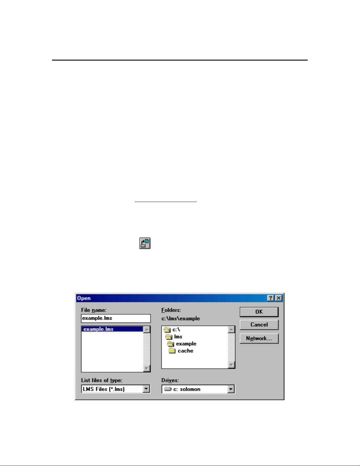
1. With LMS running, select File|Open Portfolio… from the LMS menu to load the Open
Portfolio dialog box (Figure 1).
Figure 1. Open Portfolio dialog box.
8
Page 16
2. Browse to the portfolio you want to open and select the Portfolio file (*.lms ) from the left
side of the dialog box.
3. Press OK to initialize and load the portfolio.
Saving a Portfolio
If any projections have been made to a portfolio then you will want to save those projections.
Select File|Save Portfolio… from the LMS menu to save the portfolio.
Closing a Portfolio
To close a portfolio without exiting LMS, the File|Close Portfolio… option can be used. If the
open portfolio has not been saved then the close portfolio option will ask if you want to save it.
Restoring a Portfolio
LMS Portfolios can be stored in an archived format when not in active use (files are stored using
the Info-Zip program). This saves hard drive space by compressing the files into a single ZIP file.
Archived portfolios can be restored and opened at a later time using the Restore Portfolio
command in LMS.
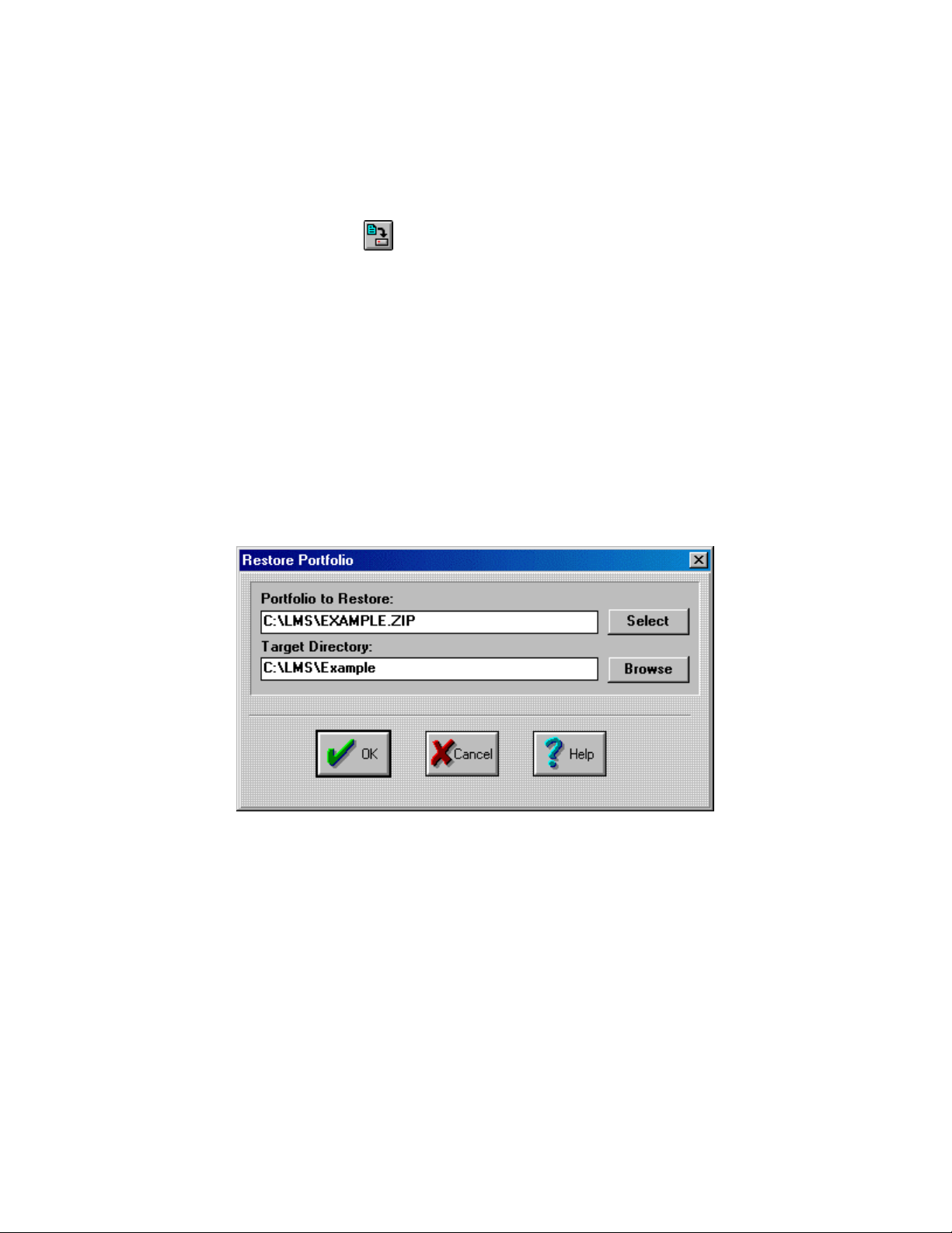
1. With LMS running select File|Restore Portfolio… from the LMS menu to load the Restore
Portfolio dialog box (Figure 2).
Figure 2. Restore Portfolio dialog box.
2. Press the Select button to load the Open File dialog (page 67) and choose a portfolio to
restore.
3. Choose which portfolio to restore. This file can be located in any directory, although LMS
defaults to the LMS directory. In this case choose the Example portfolio archive
(example.zip) and press the OK button. The path and name of the archive should appear
in the “Portfolio to Restore:” line.
4. Press the Browse button to choose the directory to restore the portfolio. Many users choose
to store the portfolios directly in the LMS directory. This clutters up the LMS directory, so it
is recommended to create a new directory off of the root (i.e. C:\Data or D:\Data) in
which to store any portfolios you use (see Appendix A on how to create directories).
Regardless, choose the directory in which you would like to store the portfolio and select OK.
5. Once you have chosen the source directory in which you want to store portfolios, add the
specific target directory for this portfolio to the end of the “Target Directory:” line. Make
9
Page 17
sure to include the slash “\” before your target (i.e. C:\LMS\Example or
C:\Portfolios\Example).
6. Select OK to restore the portfolio. Once the LMSCMD.PIF file finishes running (it will
appear on the start bar when it starts running and then disappear when finished) press OK on
the LMS Status dialog box. LMS will automatically load the restored portfolio when
finished.
Backing up a Portfolio
This function compresses all of the files in the portfolio directory into one zip file (*.zip ). This
makes it easy to transfer a portfolio from computer to another, or to save disk space when a
portfolio is not in active use.
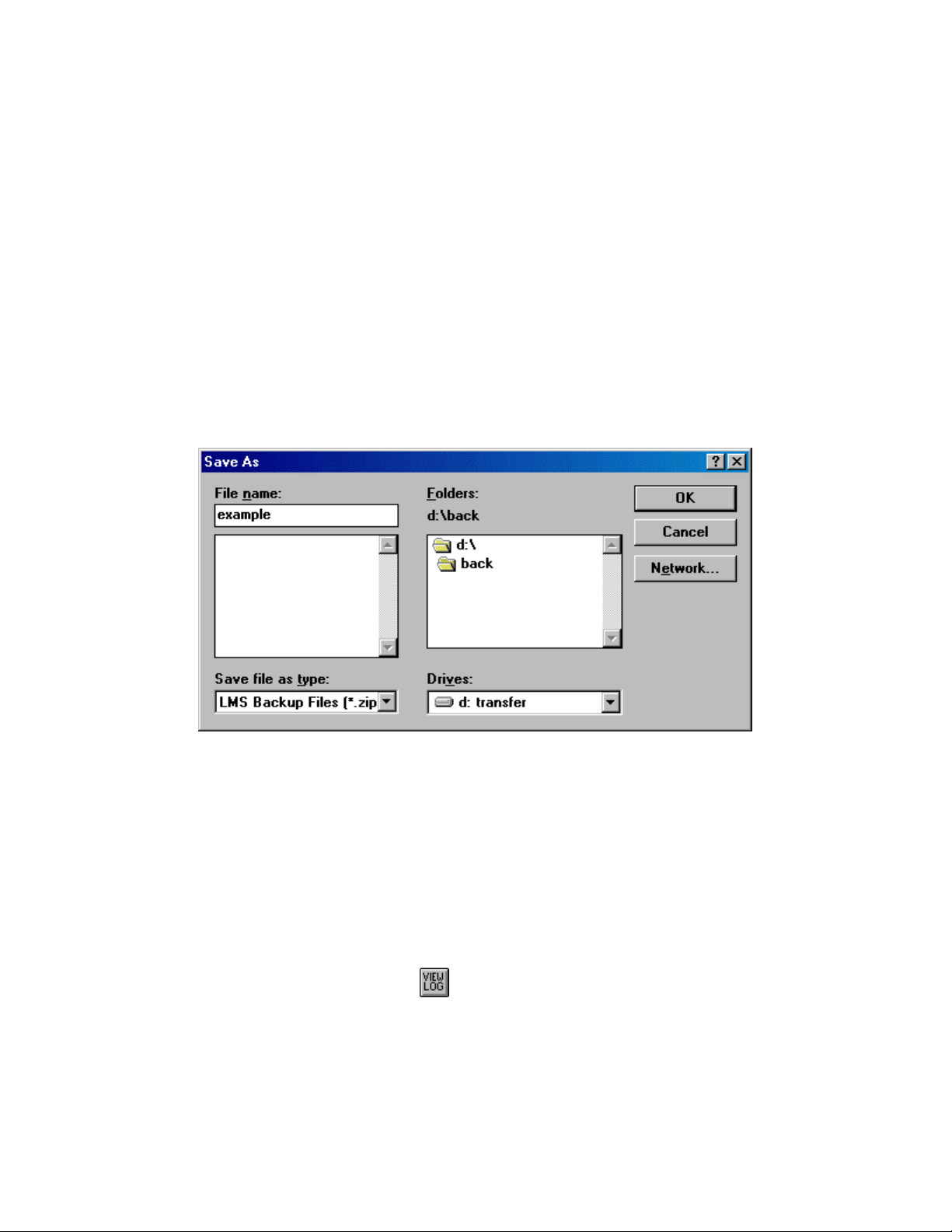
1. With LMS running and the portfolio you want to backup opened (see Opening a Portfolio,
page 8), select File|Backup Portfolio… from the LMS menu. This will load the Backup
Portfolio dialog box (Figure 3).
Figure 3. Backup Portfolio dialog box.
2. Browse to the directory you want to save the compressed file. The dialog box defaults to the
LMS directory, but it is advised to save the file to another directory to prevent clutter in the
LMS directory.
3. Select a name for the compressed file in the “File Name:” line of the dialog box (you do not
have to include the .zip extension).
4. Press OK to compress the portfolio files. Note that LMS does not close the portfolio, nor
does it remove the files from the hard drive. This must be done manually through Windows
(see Appendix A).
5. Once the LMSCMD.PIF finishes running you must press OK on the LMS Status dialog box.
Viewing the Portfolio Log
As projections and treatments are performed they are recorded in the Portfolio Log. To view the
log, use the View|View Log… function. This will load the log file into the default text editor
(Figure 4). To change the default text editor, see Configuring the Landscape Management System
(page 48).
10
Page 18
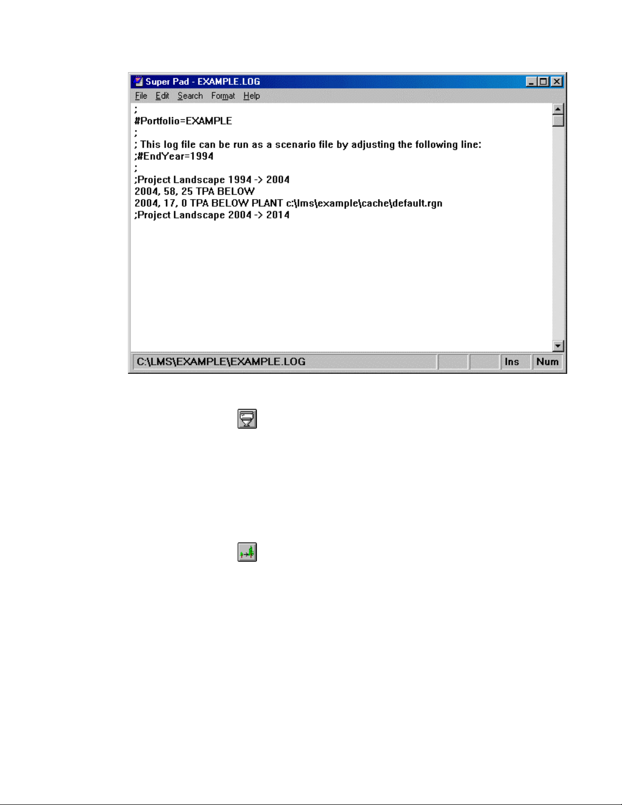
Figure 4. Portfolio Log.
Flushing the Cache
When projection and treatments are performed on a landscape the inventory files are updated to
reflect this. To restore the portfolio to its base or original status use the Utility|Flush Cache
function. Note that this will remove all of the projections and manipulations performed up to that
point.
Projecting Stands and Landscapes
This section describes those functions that project stands and landscapes forward in time.
Projecting Stands
Stand projection moves one stand forward one “stepsize” in time. The stepsize is defined when
the portfolio is created and is the number of years that projections simulate. When stands are
projected forward both the initial information and the simulated information is maintained for
analysis purposes.
1. With LMS running, select the Project|Stand… command from the LMS menu to load the
Stand Selection dialog box (Figure 5).
11
Page 19
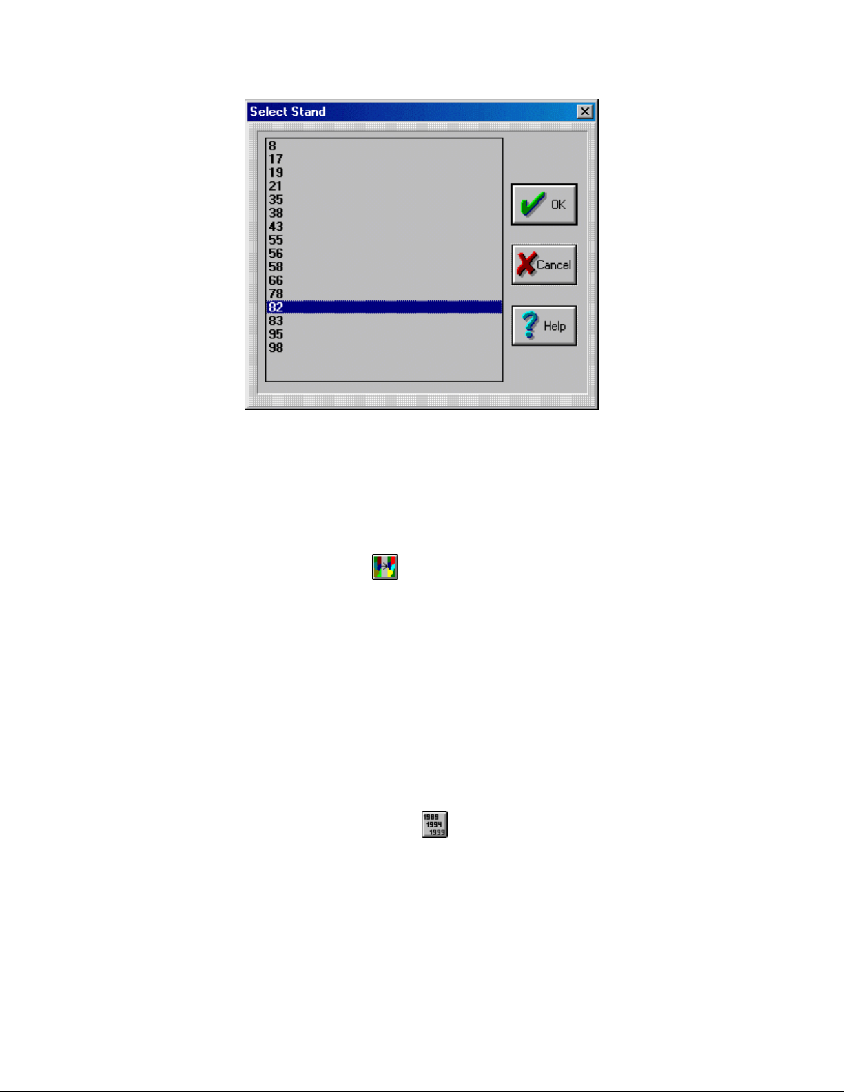
Figure 5. Stand Selection dialog box.
2. Select the stand you wish to project forward in time and press the OK button to start the
growth model.
3. When the LMSCMD.PIF finishes running press the OK button on the LMS Status dialog box.
4. Notice that the end year for the data has changed in the LMS Main Window, but because only
one stand was projected forward it will be the only data available in the future periods.
Projecting Landscapes
While it is possible to project single stands forward in time, the purpose of the Landscape
Management System is to help in managing landscapes. So, it is often necessary and desirable to
project the entire landscape simultaneously. As with the stand projections, the original and future
data are both preserved for analysis.
1. With LMS running, select the Project|Landscape… command from the LMS Menu to start
the growth model. Note that if you have just projected a single stand forward in time your
current year is sometime in the future where you may not have data for the entire landscape.
See the Changing Current Year section (see below) on how to select a time period where the
data set is complete for the landscape.
2. When the LMSCMD.PIF file finishes running press the OK button on the LMS Status dialog
box.
Changing the Current Year
When performing projections the current year for the portfolio is updated to the end of the last
projection. This makes it easy to continue making projections into the future. If however a
treatment performed did not have the desired effect it is necessary to go back to that time period
and re-project.
1. With LMS running and the Example portfolio open, select Project|Set Year… from the menu
to open the Select Year dialog box (Figure 6).
12
Page 20
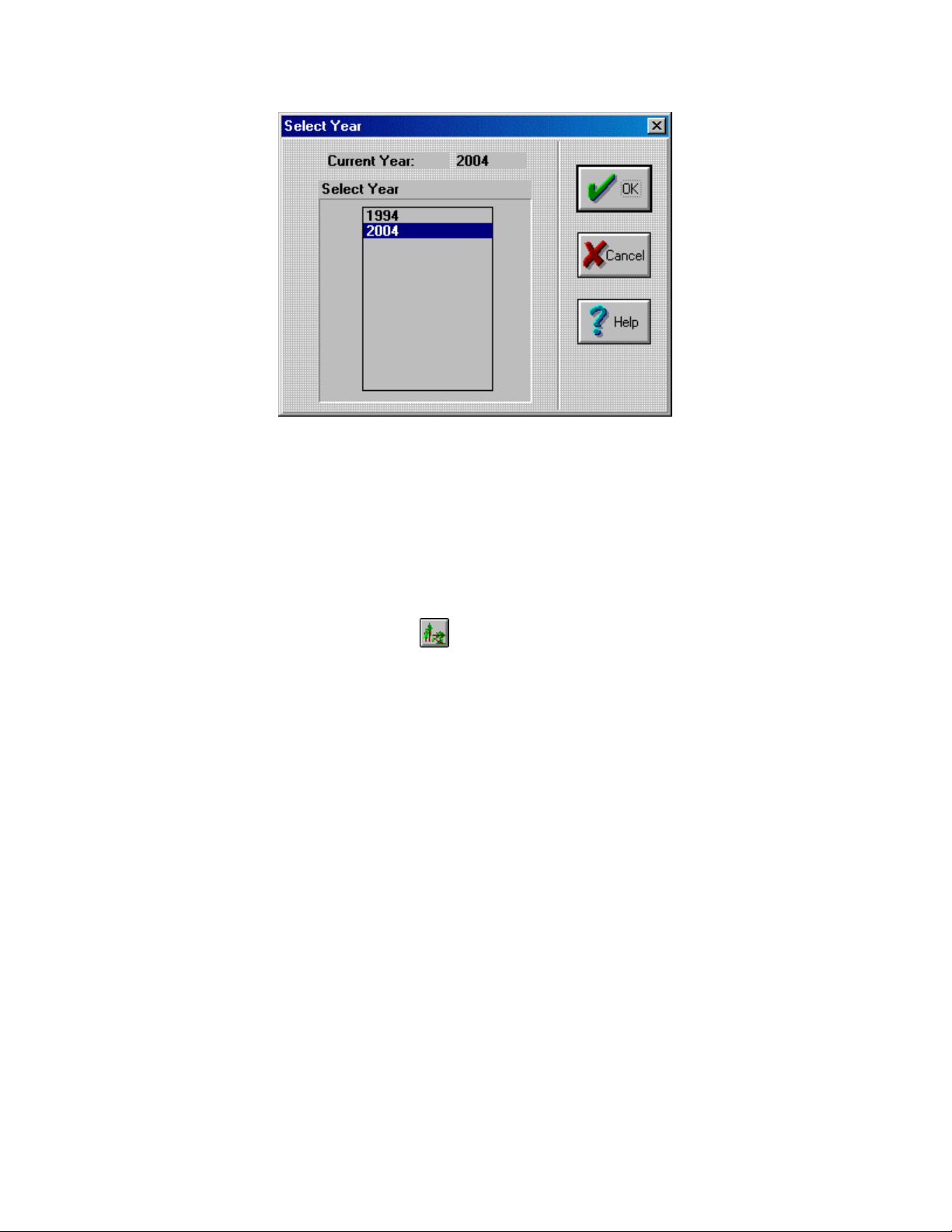
Figure 6. Select Year Dialog Box.
2. Select the year you want to go back too.
3. Press OK to change the current year.
Treating Stands and Landscapes
This section discusses those functions used for treating stands. This is a major portion of the Landscape
Management System and this section is one that should be examined closely to get an understanding of
how to effectively use LMS.
Treatment Dialog Box
Treatments are prototyped using the Treatment dialog box ( Figure 7), and may be later included in
a scenario file (page 29). All treatments, except for planting, are performed on the current year’s
data. Regeneration planted in LMS is established in the next time period, so all regeneration files
reflect trees that are one time step old.
13
Page 21
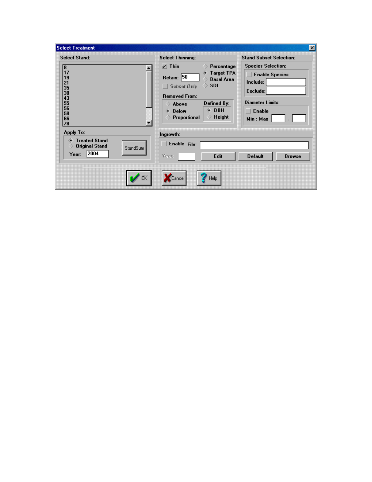
Figure 7. Treatment Dialog
The various parts of the dialog box are:
Select Stand
Highlight (by clicking on them) the stands that should be treated using the treatment you specify
in the dialog box. Note that more than one stand can be selected and treated.
Select Thinning
If the thinning option is enabled (by checking the box in the upper left corner) then the stand will
be thinned according to the parameters specified in this section.
Retain – This specifies what the remaining inventory will be. It can either be Percentage,
Target TPA (Trees per Acre), Basal Area, or SDI (Stand Density Index)
depending on what option is selected.
Removed from – These options specify how LMS determines what trees to remove from
the stand inventory. Above, below, or proportional can be by either DBH
(diameter at breast height) or by tree height depending on which option is
selected. Above removes those trees that have a larger DBH or height. Below
removes those with a smaller DBH or height. Proportional removes evenly from
across the spectrum of DBH’s or heights.
Stand Subset Selection
Often it is desirable to treat only one species or range of diameters in a stand. An example would
be removing Red Alder from a stand to favor conifers. There are two different ways to subset the
stand selected, they can be used independently or in unison. Enable either by checking the box
next to the function.
Species Selection – This option allows specific species to be treated or ignored in the
treatment. Species to ignore should be added to the “Exclude” area, while those
to treat should be added to the “Include” area. If there is a species listed in the
“Include” area then that will be the only species on which LMS will perform the
operation. Species must be specified using whatever codes the growth model
14
Page 22

uses. These must be determined from the documentation for each growth model
(FVS uses two letter species codes in upper case).
Diameter Limits – This option allows trees that fall within the specified diameter range to
be treated. The diameters should be specified in whatever units the inventory
file is using, but usually inches.
Ingrowth
The ingrowth section allows stands to be replanted using a specified regeneration file (*.RGN).
The format of this file is discussed in the File Formats section (page 56). Note that any file
specified here will be added to the inventory in the following decade (i.e. if a stand is planted in
1994 and the step size is 10 years, the regeneration will appear in 2004). So the regeneration must
reflect 10 year old trees. There should be at least 10 lines in any regeneration file, but the more
present the better.
Figure 8. Regeneration File.
Edit – opens the specified regeneration file in the default text editor. If a file is not
currently specified then the default regeneration file is loaded. To change the
default regeneration file see the Configuring the Landscape Management System
(page 48).
Default – sets the regeneration file to the default.
Browse – opens the Open File dialog box (page 67) to locate a regeneration file stored on
the hard drive.
Apply To
This section contains four miscellaneous functions simplifying the use of the treatment dialog.
Most users will rarely use most of these functions, but for completeness they are discussed here.
Treated/Original Stand – This allows treatments to be made sequentially to a stand
(treated stand option), or to throw out the previous set of treatments and use the
original stand data (original stand option).
Year – Specifies the year on which the treatment will be performed. Note that the stand
you select must be projected to the year you wish to perform the treatment. If
you select a previous year on which to perform the treatment, then you must reproject that stand forward in time. Performing the treatment will modify only
the specified year’s data.
Stand Sum – Creates the stand summary table for the selected stands. This table is a good
source of information about the stands’ current conditions.
15
Page 23
Specific Examples of Treating Stands
While the previous section explained the pieces of the treatment dialog, true understanding of how
to use the dialog box comes through use. This section gives very specific examples of how to use
the treatment dialog box to perform treatments to stands. Simulate natural disturbances using
thinnings.
Note: When performing these examples, flush the cache between them. For information on
flushing the cache see Flushing the Cache (page 11).
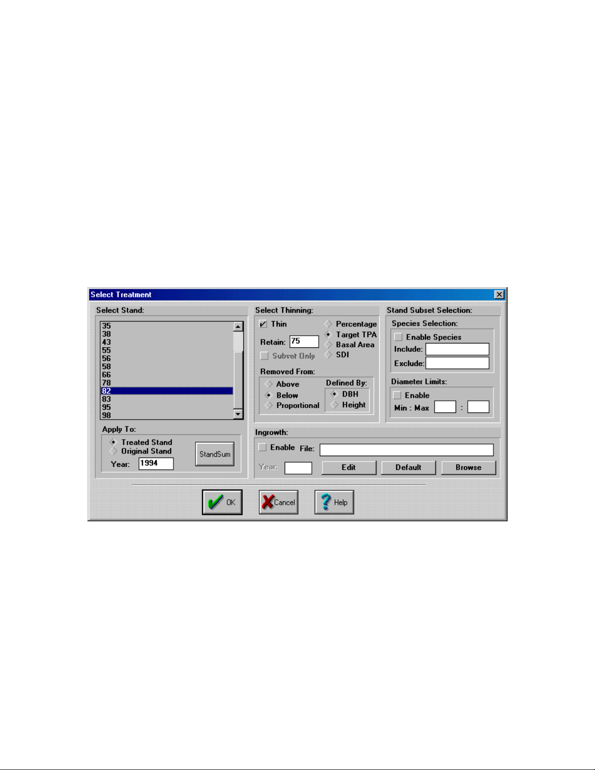
Thinning a Stand
The main function of the Treatment dialog box is to perform thinnings on stands, while many of
the other functions allow users to specify which trees to thin. In this example we will be thinning
stand 82 of the example portfolio to 75 trees per acre from below by DBH.
1. With LMS running and the Example portfolio open, select Project|Treat Stands…
to open the Treatment dialog box (Figure 7).
2. Select stand 82 in the stand selection section. Change the retain value to 75, and
verify that the “Target TPA” option is selected (Figure 9).
Figure 9. Thinning a stand.
3. Click OK. When the LMSCMD.PIF file finishes running the treatment is complete.
Vegetation Control
Stands managed for merchantable timber are often thinned to remove any unwanted species. In
western Washington, this typically involves removing Red Alder, Big Leaf Maple, and possibly
Western Hemlock depending on the density. In this example we will remove 90% of the Red
Alder and Big Leaf Maple from stand 82 of the Example portfolio.
1. With LMS running and the Example portfolio open, select Project|Treat Stands… to open
the Treatment dialog box (Figure 7).
2. Select stand 82 in the stand selection section. Change the retain value to 10 and select the
Percentage treatment option (Figure 10).
16
Page 24
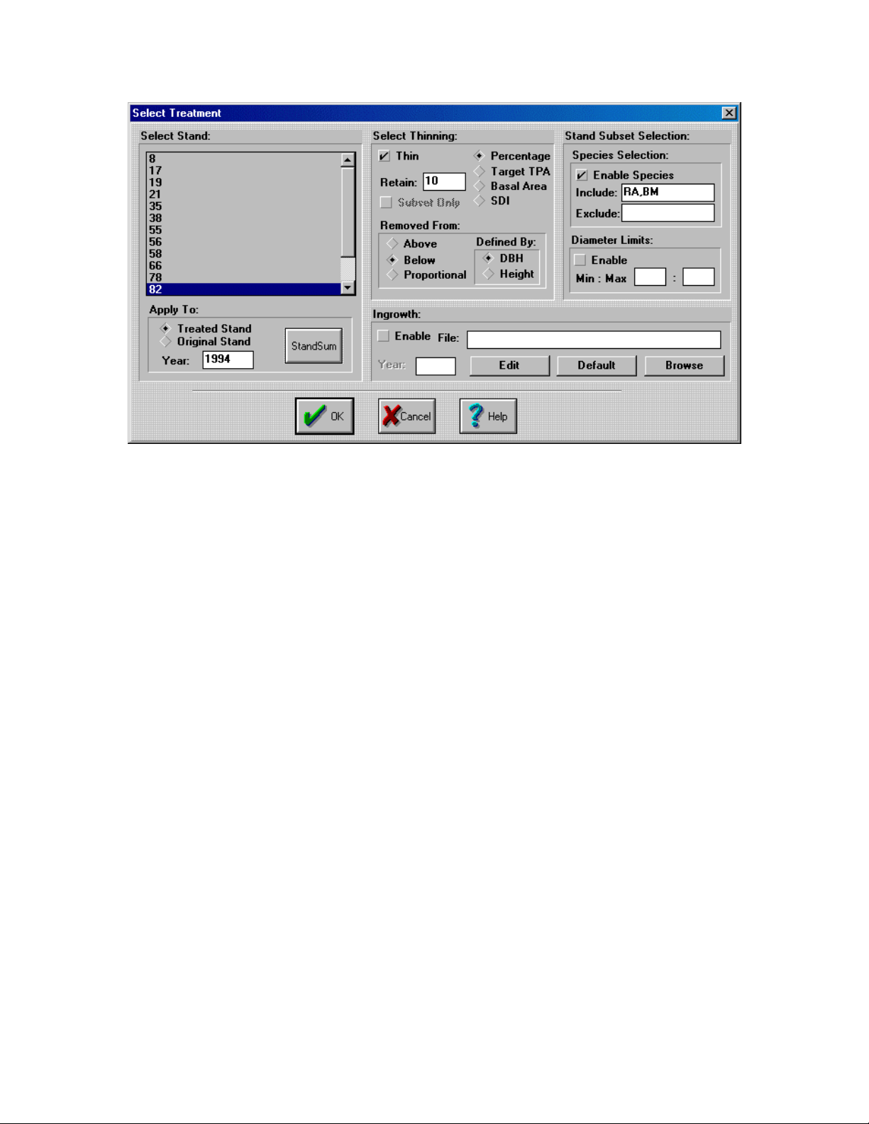
Figure 10. Vegetation Removal.
3. Click the check box next the Enable Species stand subset option.
4. Enter the species codes for Red Alder (RA) and Big Leaf Maple (BM) into the Include edit
box.
5. Click OK. When the LMSCMD.PIF file finishes running the treatment is complete.
Regenerating a Stand
In order for a stand to regenerated it must be specified as a treatment. This can done as part of the
treatment which thins the stand or as a separate treatement. In this example we will first remove
all of the trees from stand 83 and regenerate using the default regenration file.
1. With LMS running and the Example portfolio open, select Project|Treat Stands… to open
the Treatment dialog box (Figure 7).
2. Select stand 83 from the Stand Selection list box. Change the Retain value to 0 and verify
that the Target TPA thinning option is selected ().
17
Page 25
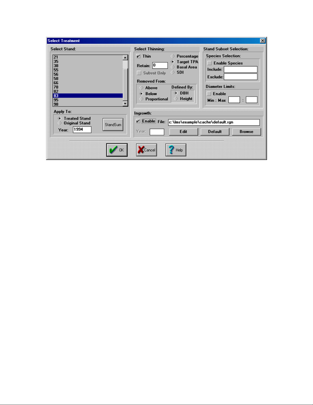
Figure 11. Regenerating a Stand.
3. Enable ingrowth by clicking the check box next to Enable in the Ingrowth section.
4. Click the Default button in the Ingrowth section to specify the default regeneration file.
5. Press OK. When the LMSCMD.PIF file finishes running the treatment is complete.
Simulating Ingrowth and Regeneration
LMS does not automatically add ingrowth to stands as projections are performed. This must be
specified as a treatment. In this example we will add ingrowth to stand 83.
1. With LMS running and the Example portfolio open, select Project|Treat Stands… to open
the treatment dialog (Figure 7).
2. Select stand 83 from the Stand Selection list box (Figure 12).
3. Disable the Thinning section by clicking the check box next to Thin.
18
Page 26
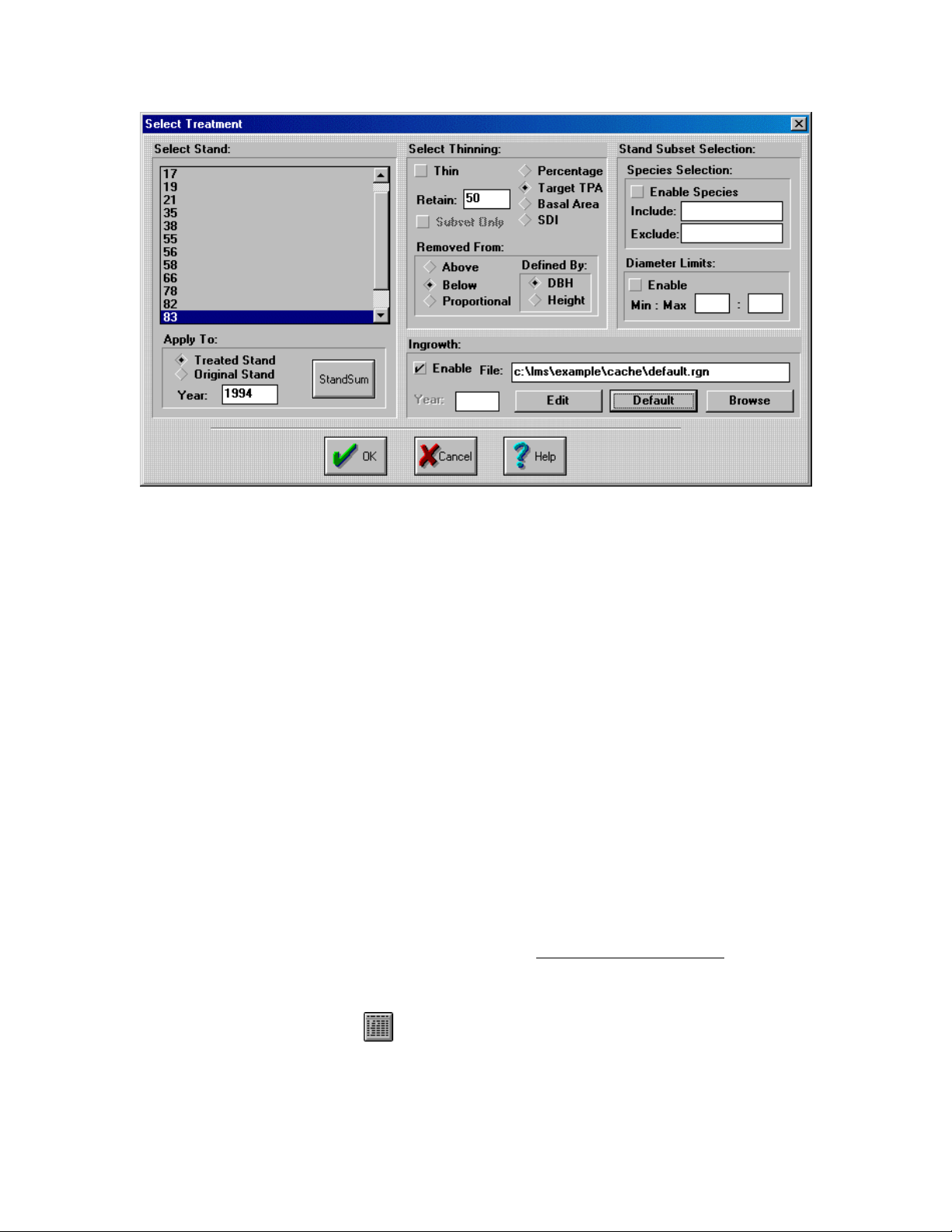
Figure 12. Ingrowth.
4. Enable ingrowth option by clicking the check box next to Enable in the Ingrowth section.
5. Press the Default button in the Ingrowth section to select the default ingrowth file. In this
example we will use the default file, but in other cases it is probably desirable to edit the file
to reflect the landscape being treated.
6. Click OK. When the LMSCMD.PIF file finishes running the treatment is complete.
Analyzing Stands and Landscapes
This section deals with those functions that analyze both the current and projected stand information in a
portfolio. The ability of LMS to perform various analysis functions allows users to determine the result of
various treatments made to the portfolio.
There are three main types of analysis that LMS can perform. The first is to summarize and display data in
a tabular format. These tables can be viewed internally within LMS or exported to another program (such
as Microsoft Excel or Access) for further analysis. The second type of analysis is a set of charts. These
charts run internally within LMS, displaying and summarizing data. The final type of analysis is the
visualization functions: stand, stand comparison, and landscape visualizations. These visualizations show a
large number of parameters inherent to each stand in a very easy to understand way.
Tables
Tables are analysis tools that provide data summarized in textual form. The tables present in LMS
have been designed to provide basic forestry statistics. It is also possible for users to add specific,
customized tables to LMS; for information on this see The LMS Programmers Guide. Tables
allow users to look at stand and landscape statistics to both determine necessary treatments and to
see the results of those treatments. The data is delimited when output and can be viewed using a
text editor or spreadsheet, or it can be saved as a file.
Table Dialog Box
The Table dialog box (Figure 13) is the interface to access all tables available in LMS. Figure 13
is the default table dialog present in LMS. If LMS has been customized, it is possible that this
dialog will show other tables not present here.
19
Page 27
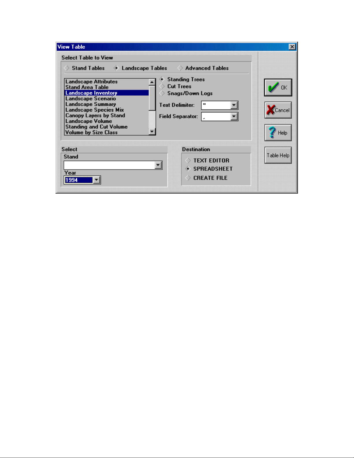
Figure 13. Table Dialog Box.
Table Type
The Stand Tables, Landscape Tables, Advanced Tables options define which of type
of table will be run. Stand tables will analyze only the selected stand, while landscape
tables look at the entire landscape. Advanced tables are those that do not comform with
either of the other groups.
Table Selection Box
This box contains a list of all the tables available. The list will be different for stand,
landscape, and advanced tables.
Data Type
The Standing Trees, Cut Trees, Snags/Down Logs options specify what type of data
will be analyzed. The Landscape Management System keeps track of standing and cut
trees and can keep track of snags/down logs as well. For further information on using
snags and down logs see the Snag Model Documentation (page 71).
Text Delimiter
This specifies what syntax will be used to specify text fields in the output tables. The
possible options are none, double quotation mark or single quotation mark.
Field Separator
This option specifies what type of field delimiter will be used in the table. The possible
options are space, tab, or comma.
Select Section
The two options in this section specify on which stand or year the analysis will be
performed. Not all tables use these values when they run.
Destination
These options specify where the table will be saved or displayed. The Text Editor
option will send it to the default text editor, while the Spreadsheet option will send it to
20
Page 28
the default spreadsheet (see Configuring the Landscape Management System, page 48).
The Create File option opens the File Save dialog box and saves the output as a text file.
Table Help Button
Opens a file that contains descriptions of each table.
Sending a Table to a Spreadsheet
In this example we will output a Landscape Inventory table for 1994 to a spreadsheet.
1. With LMS running and the Example portfolio open, select View|Tables… to open
the Table dialog box (Figure 13).
2. Select the Landscape Tables option and the Landscape Inventory table from the
Table Selection box (Figure 13).
3. Select 1994 from the Year Selection drop down box.
4. Select the Spreadsheet option from the Destination section.
5. Press OK. When the LMSCMD.PIF file finishes running press OK on the LMS
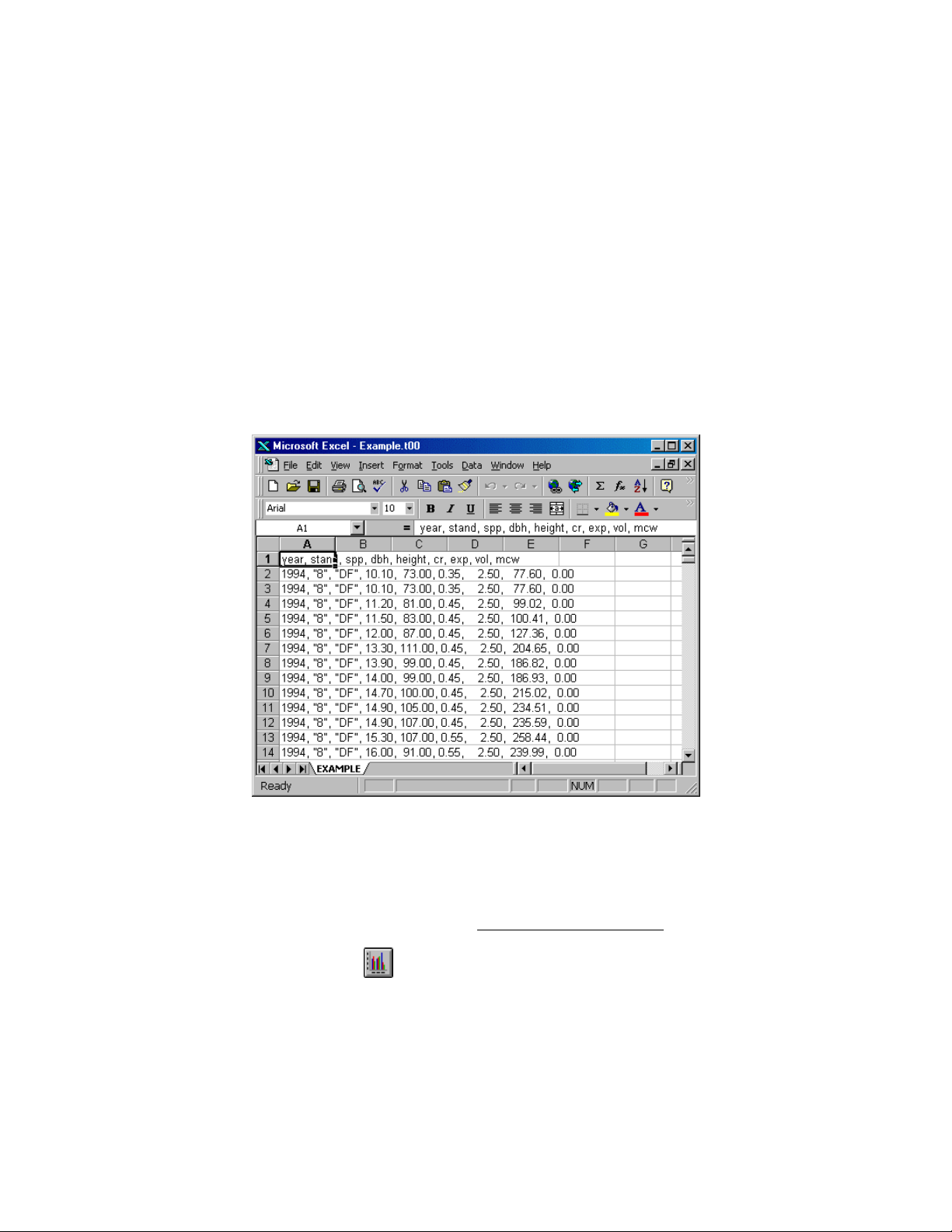
Status dialog box. The output should be similar to Figure 14.
Figure 14. Landscape Inventory table.
Charts
Charts are analysis tools that summarize data in a graphical format. Charts provide an excellent
way to summarize data over time and show trends. Like the tables in LMS, Charts can be added
and customized to reflect specific needs, see The LMS Programmers Guide.
Chart Dialog Box
The Chart dialog box (Figure 15) is the user interface to all the charts available in the Landscape
Management System. This is the default chart dialog box used in LMS, the actual dialog may be
different.
21
Page 29
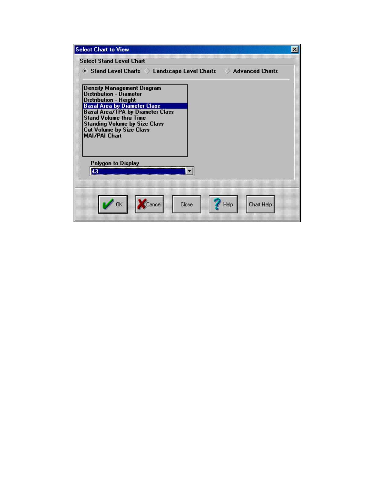
Figure 15. Chart Dialog Box.
Chart Type
The Stand Chart , Landscape Chart, and Advanced Chart options specify what type of
chart LMS will run. Like the Table dialog box (page 19), stand level charts summarize
information for one selected stand, while landscape level charts summarize the entire
landscape.
Chart Selection
This list box shows all of the charts of a specific type available in your version of LMS.
Only one chart can be selected at a time.
Polygon Selection
The Polygon to Display drop box specify which stand will be summarized when running
a stand level chart.
Close Button
The Close button closes any open chart windows in LMS.
Chart Help Button
Opens a file that explains the function of each chart available in your version of LMS.
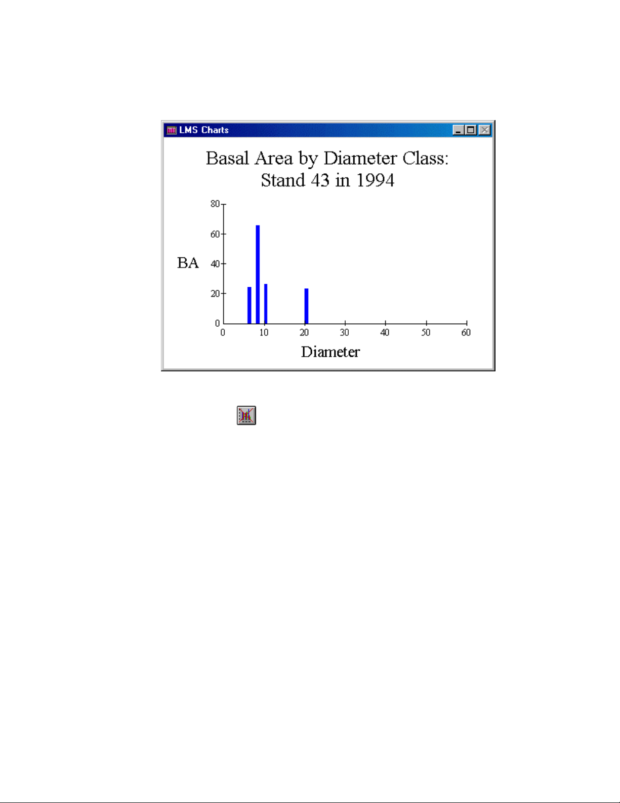
Displaying a Chart
In this example a Basal Area by Diameter Class chart will be run on stand 43 of the Example
portfolio.
1. With LMS running and the Example portfolio open, select View|Charts… to open the Chart
dialog box (Figure 1).
2. Verify that the Stand Charts option is currently selected (Figure 15).
3. Select the Basal Area by Diameter Class chart from the Chart Selection list box.
22
Page 30
4. Select stand 43 from the Polygon Selection drop box.
5. Press OK. When the LMSCMD.PIF file finishes running press OK on the LMS Status dialog
box. The results should be similar to those in Figure 16.
Figure 16. Basal Area by Diameter Class chart for stand 43.
Closing Charts
When charts are open in LMS you must use the Close Chart Window function in LMS. With
LMS running and a chart window open, select View|Close Chart to automatically close the
window.
Visualizations
Visualizations are a second way to summarize data graphically, by creating an image of the stand
or landscape. Visualizations summarize a large number of parameters in a very easy to understand
format. This makes visualizations very helpful in showing the results of various treatments to
stands and landscapes.
There are three different types of visualization: stand, stand comparison, and landscape
visualizations. Stand visualizations are performed by two versions of the same program, both of
which are distributed with LMS. SVS is a DOS version of the stand visualization program which
runs slightly faster on most machines, but will not work on Windows NT. WinSVS works on all
Windows 95/98/NT machines and is a Windows version of the stand visualization program.
Landscape visualization is performed by UVIEW, a DOS program distributed with LMS.
Stand/Stand Comparison Visualization Note: If the trees are rendered using unrealistic colors
then one of three things have occurred. The first possible explanation is that the species of tree
you are attempting to visualize is not a known species to SVS (this should not happen using the
Example portfolio). To fix this problem see the SVSLib Help File. The second possible
explanation is that you are using Windows NT which cannot use the standard SVS program to
visualize stands. However this can be fixed by changing the stand visualization program from
23
Page 31

SVS to WinSVS. To change this options see Configuring the Landscape Management System
(page 48).
Landscape Visualization Note : There are several possible problems in performing landscape
visualizations. The simplest is if LMS is being run on Windows NT, landscape visualization will
not perform correctly (it will run in 640x480 – 16 color resolution). Another possible problem is
that the size of the inventory may be too large for UVIEW to display. There are a number of
options that can be changed to correct this problem. See Changing the Visualizations Display
Options (page 49).
Stand Visualization
A stand visualization creates a flat, one-acre representation of a stand based on the inventory data.
Stand visualizations are helpful in showing differences in tree species compositions, sizes, and
spatial characteristics as treatments are performed. One important consideration is that the
position of the trees across the acre is random, and will change each time the visualization is run.
In this example we will perform a stand visualization on stand 82 in 1994.
1. With LMS running and the Example portfolio open, select View|Stands… to open
the Stand Selection dialog box (Figure 17).
Figure 17. Stand Selection dialog box.
2. Select stand 82 and press OK (Figure 17).
3. If the selected stand has been projected forward LMS will load the Year Selection
dialog box (Figure 18). Select the year you wish to visualize and press OK .
24
Page 32

Figure 18. Year Selection dialog box.
4. The Stand Visualization System will load and display an image of the stand
(Figure 19).
Figure 19. Stand Visualization of stand 82.
5. When finished viewing the image press QUIT to exit the program. For
information on how to save images see Saving Images from SVS (page 55).
25
Page 33
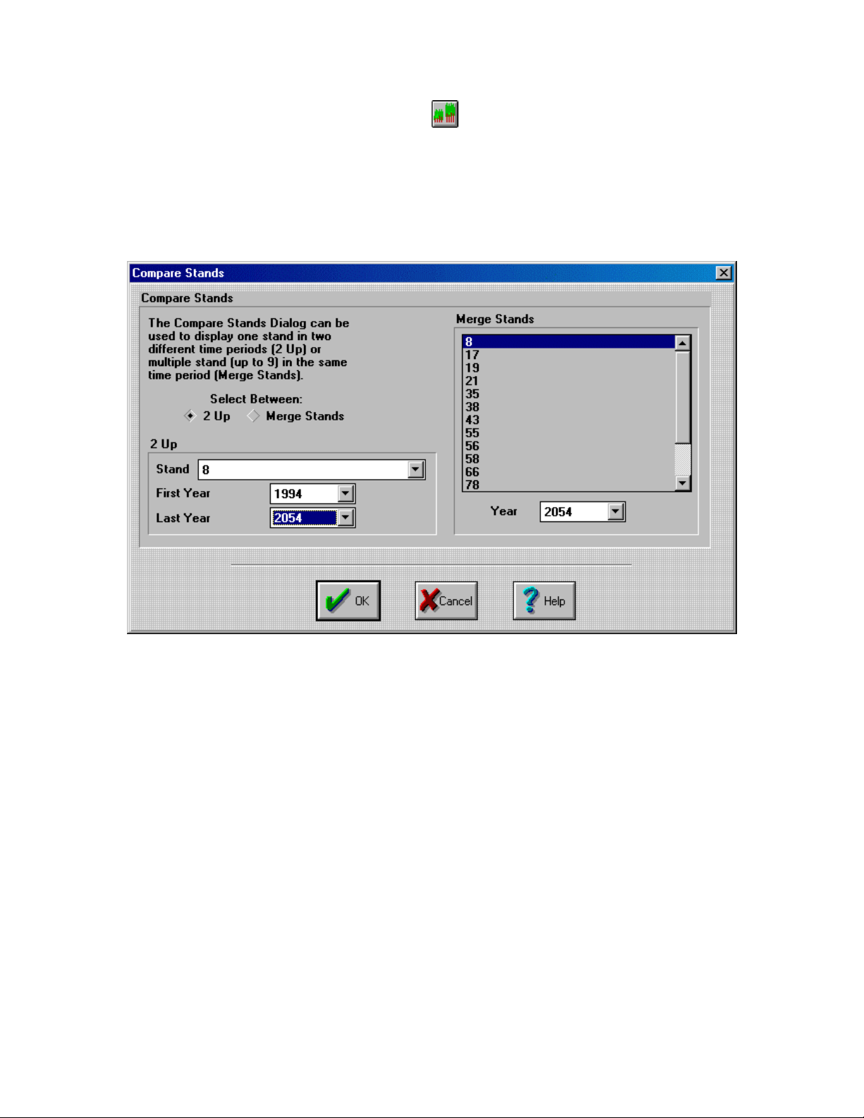
Stand Comparison Visualization
This type of visualization can compare stands by either showing two time periods side by side, or
by merging two stands together. These two types of visualizations allow visual comparisons to be
drawn between the different stands. This makes differences readily apparent.
Stand Comparison Dialog Box
The Stand Comparison dialog box (Figure 20) is the interface for performing these
visualizations.
Figure 20. Stand Comparison Dialog Box.
Visualization Type
The 2 Up and Merge Stands options select between the two types of visualization.
2 Up
These three options setup the visualization. The Stand Selection drop box
selects which stand will be visualized. First Year and Last Year are wildcard
values that LMS will lookup and use when performing the visualization.
Merge Stands
The Merge Stands list box allows up to nine stands to be selected for merging.
The Year Select determines which year will be used for the visualization.
Showing the Same Stand in Two Time Periods
Displaying the same stand in two different time periods allows users to draw visual
comparisons for before and after treatments and growth projections. Again the visual
nature of this type of analysis makes it extremely useful. In this example we will
compare stand 8 in 1994 and in 2054. For this example stand 8 must be projected
forward to 2054.
26
Page 34

1. With LMS running and the Example portfolio open, select View|Compare Stands…
to open the Compare Stands dialog box (Figure 20).
2. Verify that the 2 Up option is selected (Figure 20).
3. Select stand 8 from the Stand Selection drop box.
4. Select 1994 as the first year and 2054 as the last year.
5. Press OK.
6. SVS will display an image of the stand in each time period separated by an opening.
The first year will be on the left, the last on the right (Figure 21).
7. When you are finished viewing the image press QUIT to exit SVS.
Figure 21. 2 Up Visualization.
Merging Stands
This type of visualization allows stands which border each other to be compared side by
side. This is useful in showing edge effects, and riparian zones. In this example we will
merge stands 17 and 82 in 1994.
1. With LMS running and the Example portfolio open, select View|Compare Stands…
to open the Stand Comparison dialog box (Figure 20).
2. Select the Merge Stands option (Figure 20).
3. Select both stand 17 and stand 82.
4. Verify that 1994 is selected.
5. Press OK.
6. SVS will display an image of the merged stand (Figure 22). The different stands will
be displayed in strips across the represented acre. Stands with similar inventories
will of course be difficult to differentiate.
27
Page 35

Figure 22. Merged Stand Visualization.
Landscape Visualization
This type of visualization displays an image of the entire landscape with a representation of the
tree cover. Landscape visualizations are helpful is showing how a landscape changes over time as
treatments create openings and species compositions change. In this example we will create a
visualization of the landscape for 1994.
1. With LMS running and the Example portfolio open, select View|Landscape… to run a
landscape visualization.
2. UVIEW will display a three dimensional representation of the landscape (Figure 23).
When finished press QUIT to exit the program.
28
Page 36
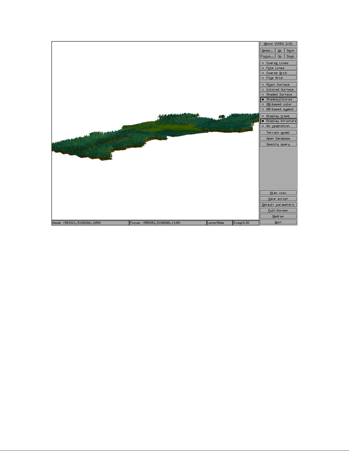
Figure 23. Landscape Visualization.
Using Scenarios Files
Scenario files provide an easy way to treat all of the stands in a landscape simultaneously through time.
The basic format of the file is a list of treatments for the stands in specific years (Figure 24). These
treatments use a keyword language shown below. Typically the treatments contained within the file are
prototyped using the Treatment Filter (page 13) and then combined for a final analysis of the effects on the
landscape. It is not necessary for a treatment to be defined for every stand in every year, only in those
years where you want to do an operation.
There are advantages of using a scenario file for the final analysis of the landscape. The first is that LMS
will perform the treatment automatically before it makes each growth projection, eliminating much of the
effort. The second is that it makes the projections reproducible. The scenario file can be re-run on the data
to get the same results. The final reason is that it is very simple to make slight changes to the scenario
file’s treatment for a stand and re-run the projection.
29
Page 37
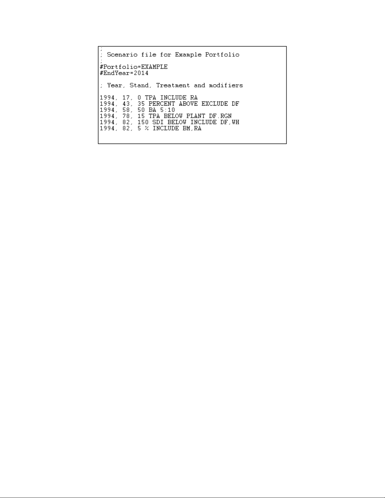
Figure 24. Scenario File Format.
Scenario File Format
The scenario file contains a header that must follow a specific format. Any comment lines are
preceded by a “;” and will not be read by LMS. The two lines preceded by a “#” are variables that
LMS uses to run the portfolio. The EndYear parameter specifies the last year of the simulation.
The Portfolio is for the user’s information only and is not currently used by LMS.
The second section of the file lists the treatments for the landscape. The first column is the year
the treatment will be performed in. The second is that stand that will be treated. The last column
is the actual treatment description. The treatment description first has the retain value (identical to
the Treatment dialog box, page 13) and then the treatment options specified using keywords.
These keywords are described below.
Note: The log file generated by LMS (page 10) can also be used as a scenario file, or treatments
within the log can be copied into the scenario file. In order to use the LMS Log file as a scenario
file you must un-comment the EndYear line (delete the “;” from the beginning of the line).
Scenario File Keywords
LMS recognizes a set of keywords in the scenario file to specify treatments. These keywords must
be spelled exactly, and must be in capital letters for LMS to recognize them. The keywords
correspond with options in the Treatment dialog box (page 13).
Thinning Type
PERCENT or % - Specifies a thinning using retain percentage.
TPA - Specifies a thinning using Target TPA (Trees per Acre).
BA - Specifies a thinning using Basal Area
SDI - Specifies a thinning using SDI (Stand Density Index).
Thinning Modifiers
ABOVE - Specifies that the thinning will be from above.
BELOW - Specifies that the thinning will be from below.
BYDBH - Specifies that DBH will be used for the ABOVE/BELOW
BYHEIGHT - Specifies that height will be used for the ABOVE/BELOW
modifiers.
modifiers.
30
Page 38

Subset Options
INCLUDE - Specifies which species will be included in the operation.
The species must follow after the keyword.
EXCLUDE - Specifies which species will be excluded from the operation.
The species must follow after the keyword.
: - Specifies a diameter range for the operation. The minumum
diameter is entered before the “:” and the maximum diameter
after it.
In LMS there are two ways to edit scenario files. The first is to use the default text editor (or any
text editor) to edit the file directly. The second method is to use the LMS Scenario Editor (see
below).
Scenario Editor
The LMS Scenario Editor provides users with an easy to use interface for creating and editing LMS
Scenario Files. The Scenario Editor has been designed to be very similar to the Treatment dialog box, so
users familiar with using that should have little problem using the Scenario Editor. The functions that will
be discussed in this section are those that are unique to the Scenario Editor, for explanations on those
functions that the two share see the Treating Stands and Landscapes (page 13).
Scenario files provide users with a way to project and treat an entire landscape at once. A scenario file
specifies the treatment for each stand in each year a treatment is made. For a further discussion of the uses
and format of scenario files see Scenario Files (page 29).
31
Page 39

Scenario Editor Dialog Box
The Scenario Editor utilizes a graphical interface (Figure 25). This section will describe the use of
each section of the dialog.
Figure 25. LMS Scenario Editor.
Scenario File Information
The top of the Scenario Editor dialog box contains information about the current scenario file and
portfolio. The only option that can be changed by the user is the End Year list box. The end year
is the year that the landscape will be projected when running the scenario file. The other options
shown in this section change with the portfolio (Portfolio, Starting Year, and Step Size) or with
the loaded scenario (Scenario).
Year and Stand Selection
This section contains two list boxes and two drop boxes that allow users to select the year and
stand they wish to add a treatment. If a Scenario file is loaded that already contains treatments
then the year list box shows all the years which contain treatments, and the stand list box shows
which stands have treatments in the selected year. The year drop box contains entries for each
valid year from the starting year to the end year (specified by the user). The stand drop box lists
each stand in the current portfolio.
32
Page 40

Treatment Selection
The treatment list box displays all the treatments defined for the selected stand in the selected
year. These treatments are displayed using the treatment keywords used by LMS, for further
information on these keywords see Using Scenario Files (page 29). Note that is possible for more
than one treatment to be defined for each year and stand combination. The treatments will be
executed from the top of the list down. The Up and Down buttons in this section change a
treatments position within the list.
Control Buttons
The block of buttons in the Scenario Editor perform all the functions necessary for creating,
modifying, and managing scenario files in LMS. Their functions are described below.
Add
The Add button appends the currently defined treatment to the selected stand
and year.
Delete
This button removes the selected treatment from the scenario file.
Replace
The replace function replaces the selected treatment with the a new one, defined
in the dialog box.
New File
Creates a new, blank scenario file. If the current file has been modified the
Scenario Editor will prompt to save the changes.
Load File
This function loads a new scenario file into memory. If the current file has been
modified the user will be prompted to save the changes.
Save File
The save file function opens the File Save As… dialog, allowing the user to
specify a location and name to save the current file. If the name and location
have already been specified during an earlier save, then those options are the
default.
About
This function loads the Scenario Editor About dialog, that displays information
on the editor.
Help
The help button loads the LMS help file for the Scenario Editor.
Change Portfolio
This function allows users to modify scenario files for other portfolios than the
one currently loaded. Note that scenario files can only be used with the
portfolio they are attached too, they are not transferable.
Preview
The preview function loads the current scenario file into the default text editor to
let a user view what the file will look like when saved. The scenario file can
also be printed from the text editor.
33
Page 41

Exit
The exit button exits the Scenario Editor. If the current file has been modified
the user will be prompted to save the changes.
Treatment Specification Section
The remaining section of the Scenario Editor is shared with the Treatment dialog box. See the
section explaining that dialog for an explanation of this section.
Using the Scenario Editor
The following examples are provided in an attempt to further explain how to use the Scenario
Editor. The examples begin with a few basic functions and progress to the more advanced
features.
Adding a Treatment
This example shows how to add a treatment to a specific stand and year. In this example we will
add a treatment to thin stand 82 to 10 TPA from below by height, and then plant the default
regeneration file in 2004.
1. With LMS running and the Example portfolio open, select the Scenario|Scenario
Editor… option to load the Scenario Editor.
2. The Scenario Editor will prompt to open an existing scenario file, press No to open the
program with a blank scenario file (Figure 25).
3. Change the End Year to 2014 (Figure 26).
34
Page 42

Figure 26. Adding a Treatment
4. Using the year drop box, select 2004.
5. Using the stand drop box, select stand 82.
6. Verify that thinning is enabled (the box in the upper left corner is checked) and set the
retain value at 10 TPA.
7. Enable ingrowth by clicking on the box in the upper left corner of the ingrowth section,
and press the Default button to use the default regeneration file.
8. Press the Add button to add the defined treatment to the scenario file.
9. Press the Preview button to see the scenario file. The program will prompt to save the
file, give it a name and press OK . The text editor then opens, it should be similar to
Figure 27.
35
Page 43

Figure 27. Adding a Treatment Scenario File
Removing a Treatment
It is often necessary to remove a treatment from the scenario file. The Delete button is designed
for just that task. In this example we will remove a treatment from the Example.scn.
1. With LMS running and the Example portfolio open, select the Scenario|Scenario
Editor… option to load the LMS Scenario Editor.
2. The program will prompt to load an existing scenario file, press Yes to open the File
dialog box.
3. The example.scn file should be available, assuming the default location for the File
dialog was correct. If the file is not present, then browse to the directory where the
Example portfolio is stored. Select the example.scn file and press OK to load the file
into the Scenario Editor (Figure 28).
4. Select 1994 from the Year list box.
5. Select stand 78 from the Stand list box.
36
Page 44

Figure 28. Removing a Treatment.
6. Select the only listed treatment in the Treatment list box.
7. Click on the Delete button to remove the treatment. Note that because this is the only
treatment for stand 78 in 1994, the stand is removed from the Stand list box.
Replacing a Treatment
When a treatment does not have the desired effect on a stand, it is often easier to change the
existing treatment than to delete it and add another. In this example we will replace the second
treatment for stand 82 in 1994 with one that removes all but 10% of the Red Alder (RA) and Big
Leaf Maple (BM).
1. With LMS running and the Example portfolio open, select the Scenario|Scenario
Editor… option to load the Scenario Editor.
2. The program will prompt to load an existing scenario file, select Yes to open the File
dialog.
3. Browse to the directory containing the Example.scn file and press OK to load the
scenario file.
4. Select 1994 from the Year list box (Figure 29).
37
Page 45

Figure 29. Replacing a Treatment.
5. Select stand 82 from the Stand list box.
6. Select the second treatment from the Treatment list box.
7. Enable the thinning option and set the retain value to 10%.
8. Enable Species Sub-selection and include Red Alder (RA) and Big Leaf Maple (BM).
9. Press the Replace button to replace the second treatment with the new one.
Portfolio Editor
The LMS Portfolio Editor is designed to simplify the task of managing portfolios. It allows users to copy
stands, remove stands, and edit the files used by the portfolio. In addition to the management of existing
portfolios, the editor is used to create new portfolios in LMS.
This section will deal with those functions used for managing existing portfolios. Information about
importing new data into LMS is available in the LMS Case Studies document.
38
Page 46

Portfolio Editor Window
The Portfolio Editor is a typical Windows program (Figure 30). For general information on how
to use these types of programs, see Appendix A (page 65).
Figure 30. Portfolio Editor Main Window
Changing the Projection Step Size
Time steps for growth projections are defined by the Portfolio Step Size variable. Most growth
models are capable of projecting tree data forward using a variety of time steps. For specific
information and limitations see the documentation for the growth model being used. In this
example we will change the step size of the Example portfolio from 10 to 5 years.
1. With the Example portfolio open, select File|LMS Portfolio Editor to open the editor
(Figure 30).
2. From the LMS Portfolio Editor’s menu select File|Modify Portfolio… to access the
Modify Portfolio dialog box (Figure 31).
39
Page 47

Figure 31. Modify Portfolio Dialog Box.
3. Change the Step Size to 5 years and press OK.
4. When you exit the editor LMS will reload the portfolio into memory and the step size
should change to reflect the new value.
Copying a Portfolio
When complex management plans are being prototyped and analyzed, it is easier to have multiple
copies of the same portfolio available for each sequence of scenarios. This allows the projections
to be saved and compared to another. In this example we will copy all the Example portfolio file
to a new directory and call it Example2.
1. With the Example portfolio open, select File|LMS Portfolio Editor to open the Portfolio
Editor.
2. From the LMS Portfolio Editor’s menu, select File|Copy Portfolio… to open the Copy
Portfolio dialog box (Figure 32). This dialog has a number of options, allowing some or
all of the files in a portfolio to be copied. The choice of which file to copy is dependent
on what the objective is.
40
Page 48

Figure 32. Copy Portfolio Dialog Box.
3. Press the Browse button to open the Select Directory dialog box ( Figure 33) to
choose the directory for the portfolio to be copied. For this example, choose a
temporary directory to store the new portfolio as you will probably not use it again.
Figure 33. Select Directory Dialog Box.
4. Choose which files should be copied by checking the box next to the type of file. Note
that the All and Clear buttons will either select all or none of the options respectively.
Press the All button.
5. Once the files have been selected and the directory specified press OK. The Portfolio
Editor will then copy the specified files to the new directory.
Copying Stands to a New Portfolio
The Copying Stands function allows users to copy specified stands from an existing portfolio to a
new one. The stand attribute and inventory information are copied for the stands, providing a way
to create portfolios that are subsets of an existing portfolio. This can be used to analyze a set of
special stands separately from the rest of the portfolio (reserves for example). In this example we
will copy stand 82 of the Example portfolio to a new portfolio.
41
Page 49
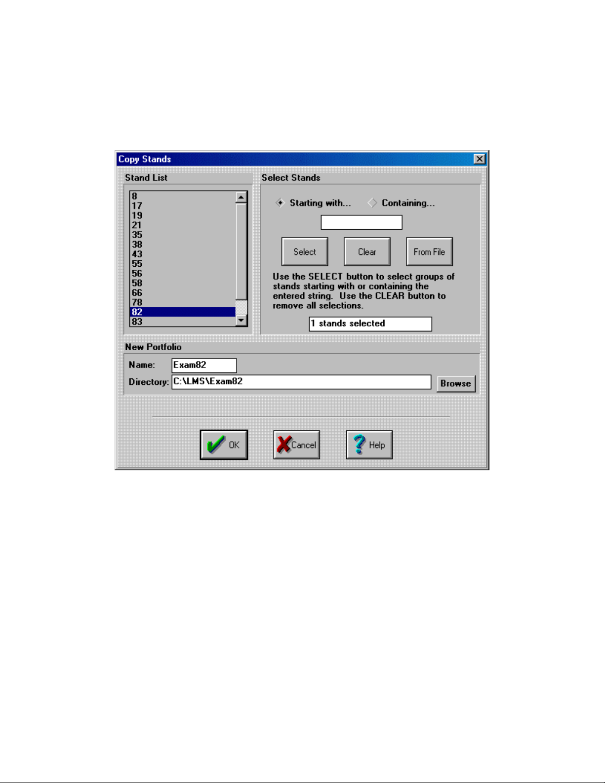
1. With the Example portfolio open, select File|LMS Portfolio Editor to open the editor.
2. From the Portfolio Editor’s menu, select Stand|Copy Stands… to open the Copy Stand
dialog box (Figure 34). This dialog has a list of stands on the left side and a search tool
on the right. You can search for stands either based a set of character in the beginning or
contained within the stand name. Alternatively you can select a stand that is contained in
another file.
Figure 34. Copy Stand Dialog Box.
3. Select stand 82 from the list of stands on the left (Figure 34).
4. Enter Exam82 for the name of the new portfolio.
5. Select an appropriate directory for the new portfolio.
6. When all the information is entered press OK . LMS will now copy the selected stand(s)
to the new portfolio.
Making Multiple Copies of a Stand
While prototyping treatments on a set of stands it is easier to run all the treatments at once rather
than separately. This requires that a portfolio contain multiple copies of the stands being treated.
The Portfolio Editor has a function to perform this task. In this example we will make 2 copies of
stand 17 from the Example portfolio.
1. With LMS running and the Example portfolio open, select File|LMS Portfolio Editor
from the menu to open the editor.
2. From the editor’s menu select Stands|Edit Stands… to open the Edit Stand dialog box
(Figure 35).
42
Page 50

Figure 35. Edit Stand Dialog Box.
3. Select stand 17 from the list box (Figure 35).
4. Press the Copy button. This will open the Rename Stand dialog box (Figure 36).
Figure 36. Rename Stand Dialog Box.
5. Enter 17-new as the copied stand’s name (Figure 36).
6. When finished press OK. The copy of the stand should appear in the list box.
Copying a Stand from another Portfolio
Another useful function is the Copy From function which is part of the Edit Stand dialog box.
This function allows users to combine two portfolios or to copy a stand from another portfolio.
1. With the Portfolio Editor running and the Example portfolio select Stands|Edit Stands…
to open the Edit Stand dialog box (Figure 35).
2. Press the Copy From… button to open the Copy From dialog box ().
43
Page 51
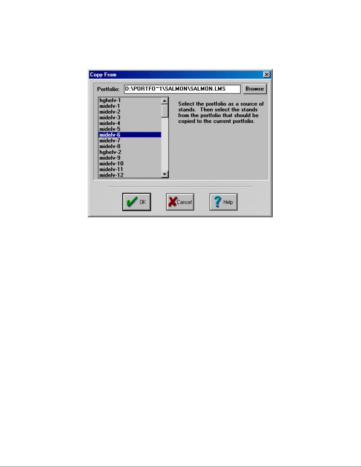
3. In this dialog you must browse to the portfolio you wish to copy a stand from. This
portfolio can be located anywhere on the current computer. Press the Browse button to
access the File Open dialog (page 67).
Figure 37. Copy From Dialog Box.
4. When you have chosen a portfolio the stands in that portfolio will appear in the list box.
Chose which stand to copy and press OK.
5. The stand will be copied to the current portfolio.
Deleting Stands from a Portfolio
Any projection of a landscape requires that every stand in the landscape be “grown.” In large
portfolios this can take a long time. To limit this time it is useful to eliminate those stands that are
not going to be part of the analysis from the portfolio. The Delete function in the LMS Portfolio
Editor removes unwanted stands. Stands can be deleted and then restored at a later date to the
portfolio. In this example we will delete stand 43 from the Example portfolio.
1. With the Portfolio Editor running and the Example portfolio open, select Stands|Edit
Stands… from the menu to open the Edit Stand dialog box (Figure 35).
2. Select stand 43 from the list box (Figure 38).
44
Page 52

Figure 38. Deleting a stand.
3. Press the Delete button.
Renaming Stands in a Portfolio
To change the name of stand in LMS use the Rename function in the LMS Portfolio Editor. Note
that if the spatial information is not updated to reflect the name change, the renamed stand will
NOT appear in Landscape Visualizations. See the LMS Case Studies for information on importing
spatial information into LMS. In this example we will rename stand 8 to stand 888 (and then
rename it back to 8 to eliminate any problems with Landscape Visualization).
1. With the Portfolio Editor running and the Example portfolio open, select Stands|Edit
Stands… from the menu to open the Edit Stand dialog box (Figure 35).
2. Select stand 8 from the list box (Figure 39).
45
Page 53
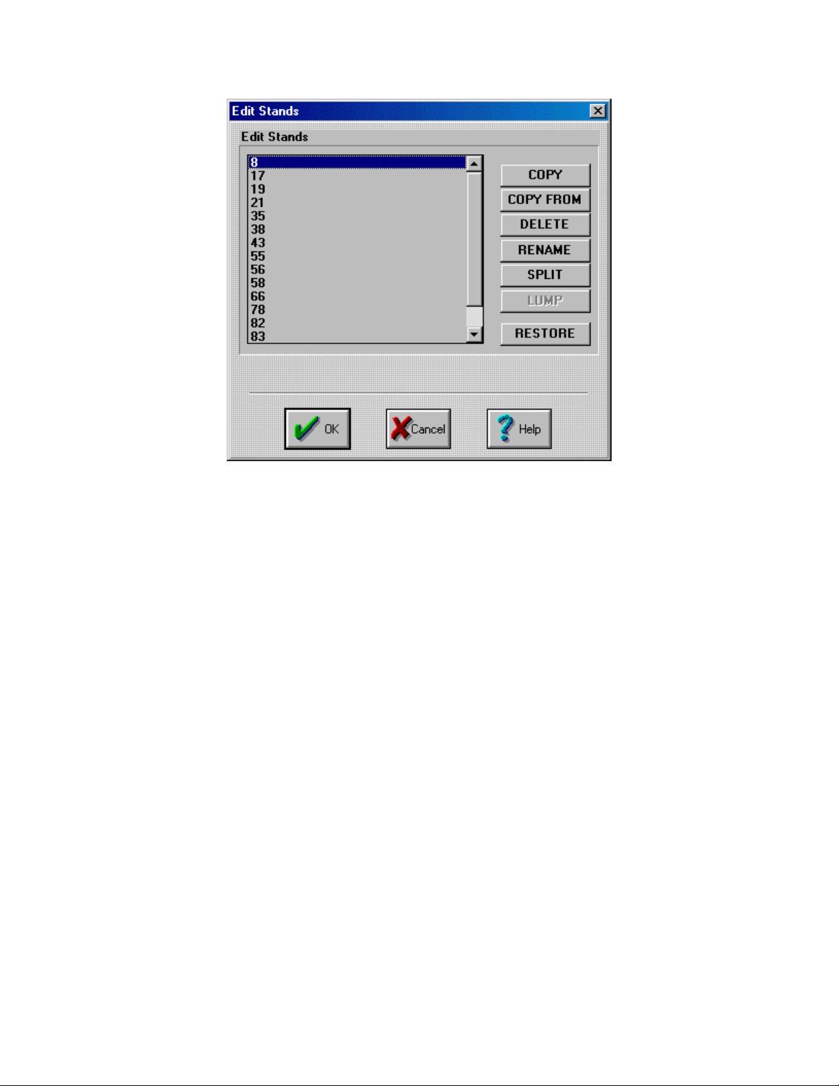
Figure 39. Renaming a stand.
3. Press the Rename button to open the Rename Stand dialog box (Figure 36).
4. Enter 888 as the new name for stand 8.
5. Press OK.
6. The list box will be updated to reflect this name change. Remember to change the stand
name back to 8 to eliminate any problems performing visualizations.
Splitting Stands
It may be necessary to split the stand inventory and stand attribute information for riparian
reserves. The Portfolio Editor’s Split function allows users to specify the area they wish to split
from the original stand into a new one. The stand attribute information is copied directly to the
new stand. In this example we will split stand 17 into a 20 acre piece and a 6 acre piece. Note
that the stand that is split from the original will not be shown in a Landscape Visualization. To
split a stand and have it appear in landscape visualizations the original GIS coverages must be
modified and re-imported into LMS.
1. With the Portfolio Editor running and the Example portfolio open, select Stand|Edit
Stands… from the menu to open the Edit Stand dialog box (Figure 35).
2. Select stand 17 from the list box and press the Split button to open the Split Stand dialog
box (Figure 40).
3. Rename the stand you wish to split from the original and define its acreage (Figure 40).
46
Page 54
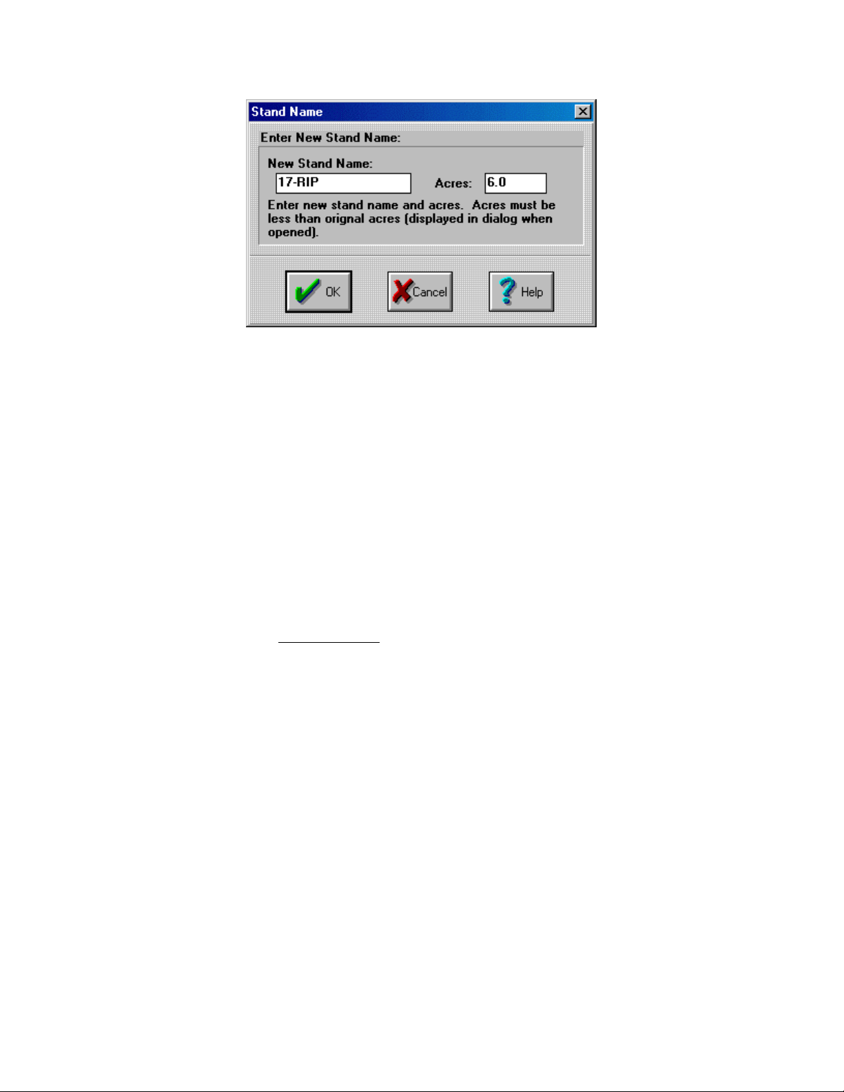
Figure 40. Split Stand Dialog Box.
4. Press OK.
Restoring the Portfolio to its Original State
After modifying the stand included in a portfolio it is easy to restore the portfolio to its original
state by using the Restore function.
1. With the Portfolio Editor running and the Example portfolio open, select Stands|Edit
Stands… from the menu to open the Edit Stand dialog box (Figure 35).
2. Press the Restore button.
Reconstructing an Inventory File
When the only inventory information available for a landscape is tree species and diameter it is
possible to reconstruct the height, crown ratio, and volume values. This is done when importing
data into LMS or when the inventory file has been modified. The Reconstruct Inventory function
is explained in the LMS Case Studies document.
47
Page 55

Advanced Topics
This section deals with configuring LMS, the formats of the various LMS files, and information about
using scenarios to manage landscapes.
Configuring the Landscape Management System
Many of the default behaviors in LMS can be modified from the LMS Configuration dialog box (Figure
41). Each of the configurable options will be discussed separately.
Figure 41. Configuration Dialog Box.
Changing the Default Text Editor
LMS by default uses the Super Pad Text editor to edit or examine ASCII files. This can be
changed to any other text editor that accepts a filename on the command line (e.g. WordPad, or
NotePad).
1. With LMS running, select Options|LMS Configuration… to open the LMS
Configuration dialog box (Figure 41).
2. Press the Browse button to the right of the Text Editor edit box to access the File Open
dialog box (page 67).
3. Find the text editor that you wish to use for editing ASCII file in LMS.
4. Press OK on the Configuration dialog. This will open the Configuration Update dialog
box (Figure 42).
48
Page 56

Figure 42. Configuration Update Dialog Box.
5. The Configuration Update dialog box allows users to specify where they want the
changes in configuration to be stored. Portfolio will only affect the current portfolio.
Defaults will change the LMS configuration file, affecting all portfolios. Both will
change both
Changing the Default Spreadsheet and Map Viewer
These two programs can be changed in the same method as the default text editor.
Displaying Snags and Logs in Visualizations
It is possible to show those trees which died in the previous projection in the visualizations. These
snags and logs will not remain on the landscape in the future unless the Snag Model is also
enabled (the next option).
1. With LMS running, select Options|LMS Configuration… from the menu to open the
LMS Configuration dialog box (Figure 41).
2. Check the box beside the Enable Snag Tracking option.
3. Press OK and choose where to update the configuration.
Enabling the Snag Model
LMS includes a model to model the presence of snags and downed logs on the landscape. It is not
necessary to have current information on snags or logs, but some tables included with LMS will
not work correctly without that information. For information on how the snag model functions, or
how to modify its behavior see the Snag Model Documentation (page 71).
1. With LMS running, select Options|LMS Configuration… from the menu to open the
LMS Configuration dialog box (Figure 41).
2. Check the box beside the Enable Snag Model option.
3. Press OK and choose where to update the configuration.
Note: The snag model will start operating during the next stand or landscape projection, any
projections previously performed will not be updated.
Changing the Visualization Display Options
Normally the display options supplied with LMS are sufficient for performing visualizations.
These values should only be changed when trees are drawn in unrealistic colors when using SVS,
or to increase/decrease the screen resolution. For an explanation of what the different modes are
for each driver, see the UVIEW Documentation (page 87).
1. With LMS running, select Options|LMS Configuration… from the menu to open the
LMS Configuration dialog box (Figure 41).
49
Page 57
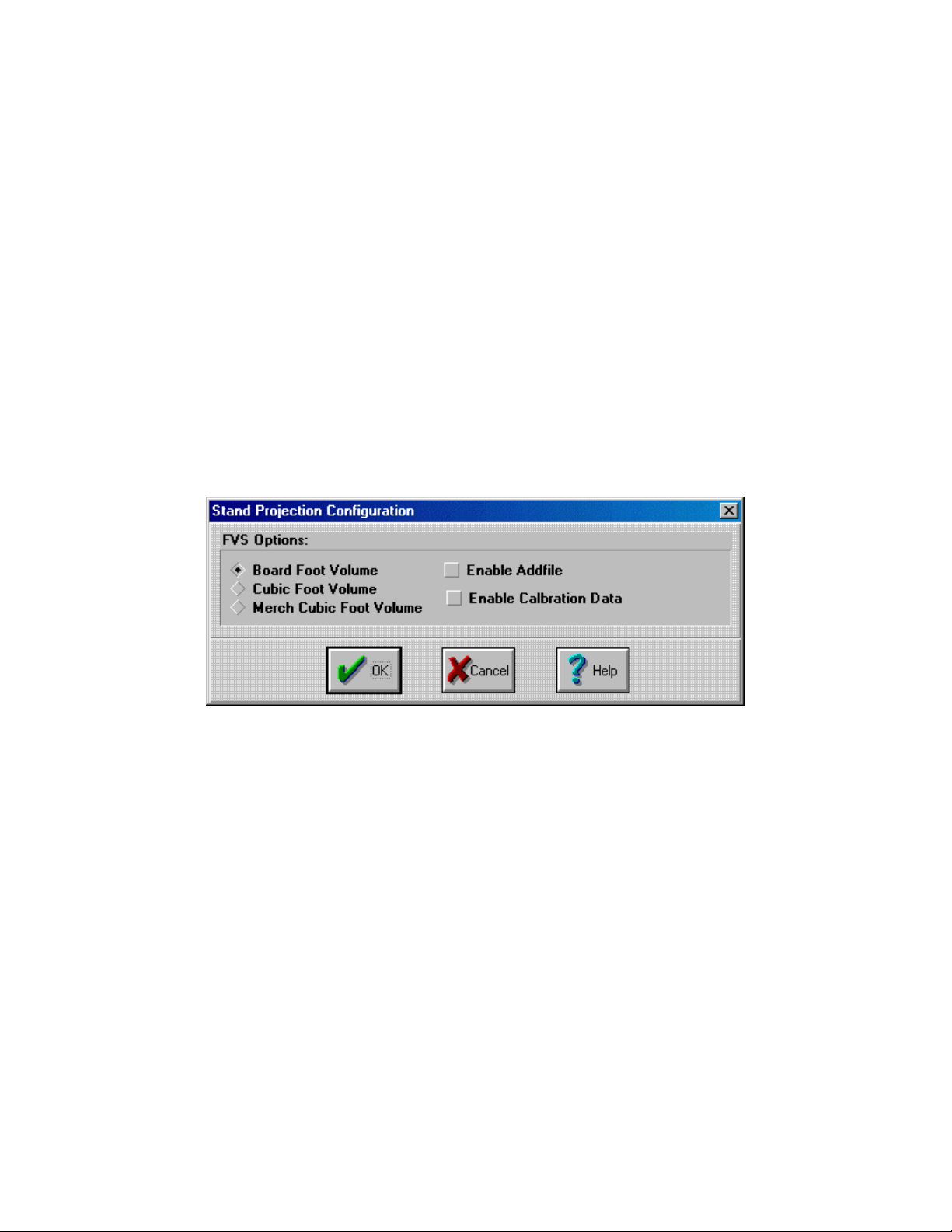
2. Press the down arrow next to the Driver option to change the BGI driver being used by
LMS.
3. Press the down arrow next to the Mode option to change the driver mode being used by
LMS.
4. Press the Test BGI button to test the selected mode and driver are valid.
5. When finished press OK and choose where to make the configuration changes.
Changing the Way Projections are Performed
The units used when performing projections, and often the behavior of the growth model can be
modified in LMS.
Changing the Units of Volume Used when Projecting
The volume in LMS can be in either Board Feet, Cubic Feet, or Merchantable Cubic Feet. The
default is to use Board Feet.
1. With LMS running, select Options|LMS Configuration… from the menu to open the
Configuration dialog box (Figure 41).
2. Press the Stand Projection button to open the Stand Projection Configuration dialog box
(Figure 43).
Figure 43. Stand Projection Configuration Dialog Box.
3. Choose what units you want the volume to be in.
4. Press OK.
Note: Not every growth model can support the different volume units. For information on
whether the growth model you are using supports different volume units, see the model’s
documentation. Also, changing the units used for projection does not change the units of any
projection already performed.
Using FVS Keyfiles in LMS
LMS has the ability to use the FVS keywords and keyfiles to modify the behavior of the FVS
growth model. An explanation of the available keywords and how to implement them in a keyfile
can be found in the FVS model documentation. These keywords can be included in the
<portfolio_name>.key file in the portfolios directory. This file may not exist and may have
to be created.
1. With LMS running, select Options|LMS Configuration… from the menu to open the
Configuration dialog box (Figure 41).
2. Press the Stand Projection button to open the Stand Projection Configuration dialog box
(Figure 43).
50
Page 58

3. Check the box next to the Enable Addfile option to cause LMS to read the
<portfolio_name>.key when performing projections.
Note: The keyfiles are used only by FVS, they will not work with any other growth model. Like
all other configuration changes, any changes made will not affect any projection performed prior
to the configuration change.
Changing the way Logs are Bucked
The LMS bucking algorithm bucks trees into logs and assigns a grade to the resulting log. The
length, top diameter, and other variables used can be updated in LMS. Any of the parameters can
be changed using the same method. For that reason only one parameter will be changed in this
example. For further information on how these parameters are used by the algorithm see the LMS
LOGVAL Documentation (page ).
1. With LMS running, select Options|LMS Configuration… from the menu to open the
Configuration dialog box (Figure 41).
2. Press the Log Sort button to open the LOGVAL Configuration dialog box (Figure 44).
Figure 44. LOGVAL Configuration Dialog Box.
3. Change the desired parameters and press OK.
4. Press OK on the Configuration dialog box and choose where you want to update the
configuration.
Adding Tree Record Numbers to Table Outputs
In order to track a tree through time it is possible to add a record number to the table outputs.
These record numbers will remain the same for the record through all time periods. This also
makes it possible to track which tree certain logs were cut from when they are bucked using the
bucking algorithm.
1. With LMS running, select Options|LMS Configuration… from the menu to open the
Configuration dialog box (Figure 41).
2. Press the Tables button to open the Table Configuration dialog box ( Figure 45).
51
Page 59

Figure 45. Table Configuration Dialog Box.
3. Enable the record number addition by checking the box next to the Include Tree
Number option.
4. Press OK.
5. When finished making configuration changes press OK and choose where you wish to
save the configuration changes.
Note: Unlike many other functions, it is not necessary to re-project the landscape in order to make
this change, it will happen immediately.
Changing How Stand Structure Classification Summarizations are Performed
When a stand structural classification is performed in LMS using the Windows 3.1x classifications
there are two options for how the information will be summarized. The first, and default, is to
summarize by stand structure. In this type of summarization the total acreage that each stand
structure covers on the landscape is output for each year. The second type of summarization is by
stand. Here each stand and its current structure are output to the table for each year.
1. With LMS running, select Options|LMS Configuration… from the menu to open the
LMS Configuration dialog box (Figure 41).
2. Press the Tables button to open the Tables Configuration dialog box ( Figure 45).
3. Change the type of summarization used by selecting the desired type from the SS
Options area of the dialog box (Figure 46).
Figure 46. Changing the Summarization Method.
4. Press OK to exit the dialog box.
5. If there are no other configuration changes you want to make, select OK from the
Configuration dialog box as well.
52
Page 60

Why the Charts & Graphs Configuration Button does not Work
This option is disabled in the LMS Configuration dialog. There are no options available at this
time.
Including Range Poles in Stand Visualizations
When viewing a stand visualization it is difficult to determine the appropriate scale of the image
because there are no objects of reference. Adding range poles in the visualization is one remedy.
The poles can be set to any height and will appear at the four corners of the visualization. In this
example we will add poles that are 75 feet in height and visualize stand 82 from the Example
portfolio.
1. With LMS running and the Example portfolio open, select Options|LMS
Configuration… to open the LMS Configuration dialog box (Figure 41).
2. Press the Stand Visualization button to open the Stand Visualization Configuration
dialog box (Figure 47).
Figure 47. Stand Visualization Configuration Dialog Box.
3. Enable the range pole option by checking the box next to Include Range Pole.
4. Change the Pole Height to 75 feet.
5. Press OK to exit the dialog box.
6. If there are no other configuration changes, press OK and choose where you wish the
changes to be made. If you perform a visualization on stand 82 the range poles should
now be present (Figure 48).
53
Page 61

Figure 48. Stand Visualizations With Range Poles.
Changing The Look Of Stand Visualizations
Many of the options used in generating the stand visualizations can be changed. This includes
items like the viewing angle for the perspective view among others. The full list of options that
can be sent to either SVS or WinSVS can be found in the LMS Help File.
1. With LMS running, select Options|LMS Configuration… to open the LMS
Configuration dialog box (Figure 41).
2. Press the Stand Visualization button to open the Stand Visualization Configuration
dialog box (Figure 47).
3. Change the desired settings and flags in the SVS Options section.
4. Press OK to exit the dialog box.
5. If there are no other configuration changes to be made press OK and choose where to
save the changes.
Defining a New Viewpoint in UVIEW
The viewpoint used to create the default Landscape Visualization can be set. This allows the exact same
point to be used for visualization each time it is performed. In this example we will create a new viewpoint
for the Example portfolio.
1. With LMS running and the Example portfolio open, select View|Landscape… to create the
Landscape Visualization.
2. Adjust the view to the desired point. See the UVIEW Documentation (page 87) for
instructions on how to change the view.
3. Once the desired view is set, press the Save Script button When the confirmation dialog box
appears, press Save Script again.
4. Select a filename for the script and press the Enter key. Press OK.
5. The file will be saved into the LMS Directory. Copy the file into your Portfolio Directory and
rename it to <portfolio>.vpt.
6. Open the renamed file in a text editor (Figure 49).
54
Page 62

Figure 49. Script File from UVIEW.
7. Delete every line except the last one. Save the changes to the file.
8. Edit the portfolio settings to include the new viewpoint file, see Using the Portfolio Editor
(page 38).
Removing the Cache
This function is similar to flushing the cache (page 11) but instead of just deleting the projections, this
function deletes the entire cache directory. Typically this function is used when you want to backup a
portfolio for storage and you don’t want to have to waste the extra space associated with the projection
files.
1. With LMS running and the Example portfolio open, select Utility|Remove Cache… to
remove the cache.
2. LMS will display a dialog box asking if you are absolutely sure. If you are press OK.
LMS will remove the cache and close the portfolio
Capturing Images from Visualizations
The images created when performing Landscape and Stand Visualizations can be saved to a file for later
editing or import into a document or presentation. UVIEW and the DOS version of SVS have identical
methods for saving the images, while the Windows version of SVS is slightly different.
Saving Images Using SVS and Uview
In this example we will save a Landscape Visualization of the Example portfolio in 1994 to the
LMS program directory.
1. Create a Landscape Visualization (page 28).
2. When you have the image manipulated to the desired view (see the Uview or SVS
Documentation for further instruction on doing this) hold the “Ctrl” key and press the
“Backspace” key. This will open the Screen Capture dialog box in either program.
3. Select to save the file as a .PCX file. Experience has shown that the .PCX format is the
simplest to use.
4. Enter testimg as the file you want to create. In the future you can also specify the
drive and directory you wish to save the file by using a DOS style command line (i.e.
C:\Temp\Donttch.pcx would save the file to drive C: in the Temp directory and
name it Donttch.pcx ). If you do not specify a drive and directory then the file will
be saved to the LMS program directory.
5. Press OK to save the image.
55
Page 63

Saving Images using WinSVS
In this example we will save a Stand Visualization image of stand 82 of the Example portfolio as
800x600 .PCX file.
1. Create a stand visualization (page 24) using WinSVS of stand 82.
2. Select File|Save image as… to open the WinSVS Save Image dialog box (Figure 50).
Figure 50. WinSVS Save Image Dialog Box.
3. Select the “Save to” File option. Choosing to the clipboard will allow you to paste the
image directly into a document or graphics editing program. Choosing to a file will save
it to the disk.
4. Select the Zsoft PCX file format.
5. Choose a 800 by 600 image size.
6. Press OK to open the File dialog box (page 67).
7. Choose a name and directory to save the image and press OK when done to save the
image.
LMS File Formats
Most of the files used by LMS are in an ASCII format, so are editable by the user. This section describes
the format of the commonly edited files. There are a few files that are not described here, they are however
described in the LMS Programmer’s Guide. For examples of how to get raw inventory data into these
formats see the LMS Case Studies document. In all of these files, comments are specified using a “;” in
front of the line in question.
Portfolio Files (*.LMS)
The portfolio file contains information on all the files and options that are part of the portfolio.
The format is show below.
56
Page 64

Figure 51. Portfolio File
The lines in this file specify:
Directory - the portfolio directory where all the files are stored.
StandTable - the Stand Database File (see below).
StatusFile - the Status File (see LMS Programmers Guide).
InitialInventory - the first year of the inventory information.
StandProjection - the growth model being used in the portfolio.
StandVisualization - the stand visualization method.
LandscapeVisualization - the landscape visualization method.
StepSize - the number of years between projection steps.
Cache - the directory where the cache is stored.
Inventory - the Inventory File (see below).
LogSortTable - the table being used for sorting logs.
DTMFile - the digital terrain model (see LMS Case Studies ).
DBFile - the paradox spatial database (see LMS Case Studies ).
ViewpointFile - the viewpoint for landscape visualization.
UW-DF - the University of Washington Douglas-fir log sort table.
FVS,PN - Forest Vegetation Simulator, Pacific Northwest variant.
SVS - Stand Visualization System.
UVIEW - Landscape visualization tool.
Stand Database Files (*.SDB)
Stand database files contain the static inventory information in an ASCII format. The format of
this file is shown below.
57
Page 65
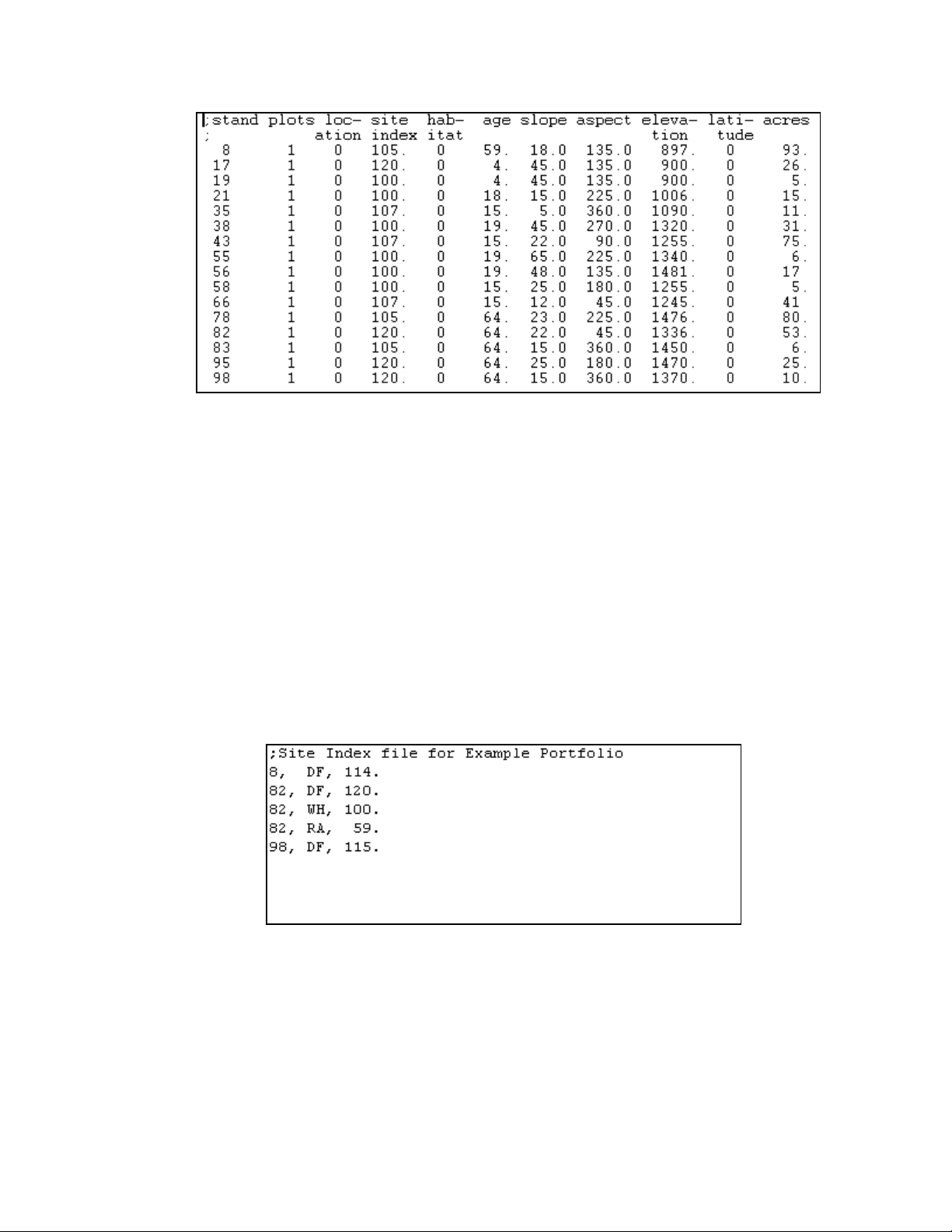
Figure 52. Stand Database File.
The Stand Database file consists of 11 columns of data. The first column is the LMS stand name,
corresponding the stand elsewhere in the program. The second is the number of plots taken to
gather the inventory information for the stand. This information is for users only, it is not used by
LMS. The third column is the location of the stand, corresponding to the location codes used by
FVS. The fourth column is the site index. This column can either be a numeric value or an “*”
which specifies that the site index values are being stored in an alternative file. The fifth column
is the habitat code, again a FVS code. The sixth is the age of stand at the initial inventory
(beginning) year. The seventh, eighth, and ninth columns are the stands slope, aspect, and
elevation respectively. The tenth column is the latitidude of the stand which is used by some
growth models to calibrate the simulations. The final column is the stand’s acreage.
Site Index File (*.SI)
Several of the growth models used by LMS (including FVS and Organon) can use species specific
site index values. LMS incorporates this functionality by using a separate file to list each stand’s
specific site index values. An example of this file is shown below:
Figure 53. Site Index File.
This file has three columns. The first is the stand, the second the species, and the final column is
the site index value. The naming convention used is <portfolio>.si and the file is used
automatically whenever it is present in the Portfolio Directory. If there is not a value defined in
this file for a species, or a stand, then the default value listed in the Stand Database File will be
used.
58
Page 66

Inventory Files (*.INV)
The dynamic inventory information for LMS portfolios is stored in an ASCII file. An example of
this file is shown below.
Figure 54. Inventory File.
Note: The ellipsis (“…”) indicates that lines have been removed from the file for display purposes
only.
The first line shown in the example is the polygon identifier. This corresponds with the stand
names in LMS. The lines between the two polygon identifiers are the individual tree records for
the first polygon.
The individual tree records can have either 7 or 8 columns of information. The first column is the
tree record, which is not used by LMS. The second column is the species code. This code is
whatever the growth model being used has for species codes. The third column is the DBH of the
tree record. The fourth is the height. The fifth is the crown ratio. The sixth is the expansion
factor, or how many trees per acre this record represents in the current stand. The seventh column
is the volume of the tree record. This is on a per tree basis and is in whatever units that LMS is
using. The eigth column, not shown here, is the maximum crown width. This is used by some of
the analysis tools for calculating canopy closure, but it is not a required variable.
Snag Files (*.SNG)
Initial snags present on the landscape are specified in the LMS snag file. The format of this file is
similar to that of the inventory file, see below.
Figure 55. Snag File.
59
Page 67

The “polygon=” line specifies what stand the following records represent. This specifier must be
identical to the LMS stand name. The records have 8 columns of data. The first is the tree record,
and is not presently utilized by LMS. The second is the species of the snag, again these codes
must correspond with those of the growth model in use. The third, fourth, and fifth represent the
snag’s diameter, height, and trees per acre respectively. The seventh column specifies whether
this record represents a standing snag, or a downed log (1 is a snag, 0 is a log). The eighth column
is the number of years since the snag was created, or the age of the snag. The final column is the
decay class the snag is in currently.
Regeneration and Ingrowth Files (*.RGN)
The regeneration files are edited by hand using a text editor (such as Notepad or Superpad). The
format is similar to the inventory files, without any values entered for the volume.
Figure 56. Regeneration File Format.
The file is divided into seven columns of information. The first column is the species code for
whatever model is being used to project the landscape. The second is the diameters of the trees
being planted. The third column is the heights of the trees, while the fourth is the crown ratios.
The final column with any values is the expansion factor for that record, or the number of trees per
acre it represents.
Notice that these values are larger those of newly planted trees. This is because the regeneration
file represents 10 year old trees, they are planted into the site at the end of the growth cycle.
Scenario Files (*.SCN) and Log Files (*.LOG)
Figure 57. Scenario File Format.
The scenario file contains a header that must follow a specific format. Any comment lines are
preceded by a “;” and will not be read by LMS. The two lines preceded by a “#” are variables that
LMS uses to run the portfolio. The EndYear parameter specifies the last year of the simulation.
The Portfolio is for the user’s information only and is not currently used by LMS.
60
Page 68

The second section of the file lists the treatments for the landscape. The first column is the year
the treatment will be performed in. The second is that stand that will be treated. The last column
is the actual treatment description. The treatment description first has the retain value (identical to
the Treatment dialog box, page 13) and then the treatment options specified using keywords. For
more information see Scenario File Keywords (page 30).
61
Page 69

Glossary
ASCII ASCII is the name of one of the character sets used on computers. The ASCII
character set was standardized by the American National Standards Institute in 1968
and revised in 1983 (ANSI X3.4-1968, ANSI X3.110-1983). When we refer to
ASCII files we are talking about text files with no special formatting characters
(other than TAB or NEWLINE). These are also known as text files.
Backup Portfolio A Backup Portfoli o in LMS consists of an archive file containing all the files
included in the portfolio directory. They are usually created using the LMS
File|Backup Portfolio... command. LMS currently uses ZIP to create the Backup
Portfolios. The example datasets are distributed as Backup Portfolio files.
BGI Borland Graphics Interface. BGI drivers are a graphics hardware interface
developed by Borland International that allow the programmer to develop to a
software specification instead of having to deal with video hardware directly.
CACHE In general, “cache” is a term used in computing as a place where frequently used
information is stored. A cache is often used to speed up access to information. In
LMS, cache is used in a similar way. All the projected inventory files and temporary
files used for growth projection and visualization are stored in the CACHE directory
tree. The name CACHE is used to indicate the temporary nature of the files.
Anything under the CACHE directory tree is transient in nature and can be deleted at
any time. Permanent information about a portfolio should be stored in the portfolio
directory.
DEM Digital Elevation Model
DTM Digital Terrain Model
Filters LMS uses many auxiliary programs to perform specific format tr anslation tasks and
to provide unknown information. All of these programs are defined as “filters” in
LMS. In general, a filter is a program that performs the task of converting one
packet of information (a stand inventory for example) into another packet of
information (maybe a stand visualization input file). Filter is the generic term used
collectively for all these programs.
FVS Forest Vegetation Simulator is an individual tree, distance independent growth
model (formerly known as Prognosis). It is developed by the USDA Forest Service
and has a variant for all of the areas of the United States where there are National
Forests.
GIS Geographic Information Systems
Landscape land••scape (land skayp) n. 1. the scenery of an inland area. 2. a picture of this.
Landscape is used to refer to a land area of interest. In the LMS context the
landscape is the elevation model that can be viewed by the landscape visualization
software.
LMS The Landscape Management System.
MS-DOS Microsoft Disk Operating System. A commonly used operating system for Intel-
based (and compatible) personal computers.
62
Page 70

Open File Dialog The Open File
Dialog is used by
many Windows
programs to locate
various types of
files. The Dialog
consists of several
regions, each
designed to select
different types of
information. To
change the disk
drive being
examined, use the Drives region to pick from the available disk drives. Use the
Directories: region to select the desired directory. Double click a folder to access the
directories in that folder. After the proper Drive and Directory have been selected,
select the desired file in the File Name region. The filename can be double clicked,
which is the same as highlighting the name and pressing the OK button.
ORGANON ORGANON is an individual-tree distance-independent growth and yield model
developed at Oregon State University. It was originally developed for Southwest
Oregon and has subsequently been calibrated for other areas.
PATH Operating systems execute programs from a variety of locations. Under MS-DOS,
this is controlled by an environment variable named PATH. The PATH is set using
the MS-DOS PATH command. When the user types the name of a program, MSDOS looks in the current directory for a match of the name. If no match is found,
MS-DOS then looks in each of the directories indicated in the PATH and executes
the first match found.
Portfolio Information in LMS is contained in a number of related files that represent a land
area. These files, along with applied projections and treatments, are collectively
called a portfolio. A portfolio includes all of the spatial and inventory files necessary
for LMS to project and visualize stands and landscapes. These files are arrayed
across a series of subdirectories contained within the home directory for the
portfolio.
Polygon also polygon identifier
Project pro-jekt (v.) versus proj-ekt (n.): In LMS the verb project (pro-jekt) is used when
discussing estimating stand conditions at a future time. The noun project (proj-ekt)
is not used in order to avoid the confusion caused by using both pronunciations.
Instead, portfolio is used for the collection of files for a particular landscape.
Scenario Combination of growth and treatments for a stand or multiple stands.
Radio Button Toggles between two or more options in a dialog box.
Raster Same as pixel. As opposed to vector.
Stand Operational unit for LMS, also called polygon.
SVS Stand Visualization System.
Tables List of information.
Text Editor Any program that allows user to read and edit ASCII files.
Treatment Any manipulation of a stand or polygon inventory, typically executed in the
Project|Treat Stands... dialog. Can include thinning, planting, and harvesting.
63
Page 71

UTOOLS Watershed analysis and visualization software package developed by the U.S. Forest
Service.
UVIEW Landscape visualization module within the UTOOLS software package.
Vector A set of connected coordinate points describing polygonal boundar ies.
VESA A video interface specification for IBM compatible computers.
*.ZIP Any file that has been compressed using Zip, WinZip or PKZip. This is a
mechanism for efficiently transferring large files or collections of files.
64
Page 72

Bibliography
McCarter, James B., Christopher E. Nelson, LMS Case Studies . Silviculture Laboratory, College of Forest
Resources, University of Washington.
McCarter, James B, 1999. LMS Programmer’s Guide. Silviculture Laboratory, College of Forest
Resources, University of Washington.
65
Page 73

Appendix A – Using Windows Programs
It is true that every program is unique in its functions and how it works, but there are many pieces of
programs designed for Windows that are similar. Users familiar with using these types of programs will
not have to read this section, but those who have not used Windows programs may want too.
This section will discuss the basic parts of the LMS program, and how to use those them. It will not go into
any depth on how to use the functions, that is contained in the earlier sections of the manual.
LMS Main Window
The main window of LMS (Figure 58) is the interface for users to perform the various functions contained
within LMS. It is made up of five basic parts which will be discussed in turn.
Figure 58. LMS Main Window.
Title Bar
The title bar gives the name of the program being used. You can close the program by clicking on
the “X” in the upper left corner (assuming you are using Windows 95/98/NT).
Also on this bar are the buttons to minimize or maximize the program. Minimizing shrinks the
program into an icon allowing the desktop to be used for other programs. This program can be
brought back by clicking on the icon. The same is true of maximizing, which blows the window
up to fill the entire screen. Neither of these functions will close the program or cause you to lose
any data.
The last item of interest is the icon in the upper right corner. This icon also provides additional
functions when clicked on with the mouse. The LMS Main Window does not place any special
functions within this icon’s menu, but other programs such as the Chart Windows (page 22) does.
LMS Menu
The menu is an easy to use straight forward way to access the functions within LMS. The
examples contained in this manual tell you where to find each of the functions within the LMS
menu. To access a menu option, just click on the word and the menu will do the rest.
66
Page 74

Speed Button Bar
The speed button bar provides a quick way to access the commonly used functions within LMS.
Throughout the manual there are pictures of the buttons contained on this bar, and the functions
that they access. Another way to determine what the button access is to hover the mouse pointer
over the button and look in the status bar for a description of the button.
Main Application Window
The large white space in the window contains all the information for the currently open portfolio.
Notice that if there is no portfolio open, then there will be no information listed.
Status Bar
The status bar at the bottom of the main window provides users with information regarding the
various buttons in LMS, and other information as the program is run. At times text will appear in
the status bar to keep the user informed of what LMS is doing.
Open and Save File Dialogs
The dialog boxes used for saving and opening portfolios and all other files in LMS are fairly general to
Windows programs as a whole. There are however differences between the 32-bit dialogs (Figure 59,
Windows 95/98/NT programs) and the 16-bit (Figure 60, Windows 3.1x and early Windows 95). These
two types will be discussed separately.
32-bit File Dialogs
The 32-bit file dialog box (Figure 59) is used primarily only in the Scenario Editor (page 29) and
any other program that did not come with LMS. Despite looking different than the 16-bit dialog,
it operates very similarly.
Figure 59. 32-bit File Dialog.
Control Bar
The control bar along the top of the dialog allows users to specify an existing directory by
pressing the down arrow in the drop box. This will show a tree of available files and
directory on the computer being used. The other functions will not be used much in
LMS, but you can find out what they are by holding the mouse over the button and
waiting for the balloon to appear.
67
Page 75

File Selection Box
The main box in the center of the dialog allows users to select files or directories by
clicking on them with the mouse. Clicking once on a file will highlight it and copy its
name to the File Name line in the dialog. Double clicking will allow you to rename the
file (not recommended). Double clicking on directories will allow you to descend into
the directory.
File Name
Put simply this is the name of the file that will be used when exiting the dialog box (may
be saving or opening). You can type a name here if you want, but typically it will have to
exist to be used.
Files of Type
Specifies what type of files will be shown in the File Selection Box . The contents of this
drop down box will change depending on what dialog is being used.
Open and Cancel Buttons
These two buttons are fairly obvious.
16-bit File Dialogs
The 16-bit dialogs (Figure 60) are used throughout most of LMS. The are very similar to the 32bit dialogs, but lack some of the functionality that the 32-bit contain.
Figure 60. 16-bit File Dialog.
File Name
This line specifies what file will be used when the dialog box is exited.
File Selection Box
This box allows users to select the file name they wish to use by clicking on the file with
the mouse pointer.
Folders Selection Box
This box allows users to browse through the various folders contained on the computer.
To descend into a directory double click on its name. To close a folder do the same.
68
Page 76

List files of type
Specifies what type of files will be displayed in the file selection box. The contents of
this drop down box will change depending on where the dialog was created.
Drives
This drop box is how to change drives when trying to find a file. Press on the down
arrow to get a list of available drives.
Creating Directories
Some functions in LMS require a directory to be created manually. The method used depends on the type
of operating system.
Windows 95/98/NT
In Windows 95/98/NT it is easiest to use Windows Explorer to create directories.
1. Start Windows Explorer (it is usually available from the Start|Programs… menu from the
Windows Start Bar).
2. Browse to the location you want to create a new directory on the left hand pane.
3. Select the File|New|Folder option.
4. Rename the folder.
Windows 3.1x
1. Start File Manager (located in the Main folder).
2. Select the File|Create New Directory option.
3. Name the directory and press OK.
69
Page 77

Appendix B – Documentation and Credits for LMS Support Programs
LMS is a tool that integrates many others. Some of the programs it integrates were written expressly for
LMS, but not all. LMS also incorporates many programs that were designed for other purposes by other
people. This section provides the documentation and credits that are due to these authors.
ADDELEV
Author: Bob McGaughey
Contact Information: mcgoy@u.washington.edu
NOTE: ADDELEV is distributed as part of the UTOOLS package.
ADDELEV is used in the conversion of spatial information for use with LMS. ADDELEV adds elevation
values to a Paradox spatial database, obtaining the values from a Digital Terrain Model. ADDELEV is part
of the UTOOLS Watershed Analysis and Visualization software.
ADDELEV version 1.0 – Syntax:
ADDELEV database DTMfile xyfld elevfld [/X# /R /C]
database name of Paradox database file...no extension
DTMfile file name for PLANS format DTM...include extension
xyfld field number for field containing XY data
elevfld field number for field to receive elevation data
/X# number of digits in X value within XY field (default = 7)
/R replace the elevation in the database with a new elevation
/C do not ask for confirmation of database fields
Example: ADDELEV udemo quad27.dtm 1 12
-Add elevation to the database named UDEMO.DB where XY value is
located in field 1 and elevation should be put in field 12. Use the DTM file
named quad27.dtm as the source of elevation data.
Figure 61. ADDELEV Help Screen.
ASC2DB
Author: Bob McGaughey
Contact Information: mcgoy@u.washington.edu
For landscape visualization, LMS needs to create a Paradox “structure” database to be used by UVIEW.
This structure database tells UVIEW how to draw trees in each cell of the spatial database. Getting the tree
inventory information into the structure database is a multi-step process that ends with the conversion of an
ASCII file into a Paradox database. ASC2DB is the program that converts the ASCII file into a Paradox
database. ASC2DB is an MS-DOS program with the following options:
70
Page 78

ASC2DB -- Revision: 1.4 --syntax:
ASC2DB ASCII_file db_file [-K -Q -H -S### -F###]
ASCII_file name of ASCII file to convert to a PARADOX table
db_file name of PARADOX table to be created
-K add a key on field 1 of the PARADOX table...duplicate values in
field 1 will cause a key violation and ASC2DB will abort
-Q suppress all screen output
-S### use decimal character ### to delimit string...default: “
-F### use decimal character ### to delimit fields...default: ,
-H display this help information
File format:
The ASCII file must conform to loosely structured format. The first
line must contain the field names enclosed in quotation marks and separated
by commas. The second line contains the field types enclosed in quotation
marks and separated by commas (A,N,S,$). The following lines contain the
data. String fields must be enclosed in quotation marks and all fields are
separated by commas.
Sample file...line 1:”Name”,”Phone number”,”Age”
line 2:”A20”,”A11”,”N”
line 3:”Sam”,”555-3212”,25
line 4:”Ralph”,”555-3412”,35
Figure 62. ASC2DB Help Screen.
BUCKTREE
Author: James B. McCarter
Contact Information: email: jmac@silvae.cfr.washington.edu
Phone #: (206)616-2376
Address: College of Forest Resources, Box 352100
University of Washington
Seattle, WA 98195
BUCKTREE examines the trees cut in each time period and bucks them into logs.
Usage: BUCKTREE [-l #] [-x #] [-m #] [-s #] [-t #] [-v] treelist.tre [treeval.lgl]
Divide tree records into a series of log records.
-l # : log length (default 16’)
-x # : exclude logs shorter than (default 0’)
-m # : minimum (top) diameter (default 4”)
-s # : stump height diameter (default 1’)
-t # : trim on each log (default 1.0’)
-v : verbose output
BUCKTREE: Version 1.3 (Apr 13 1999 – 10:27:47), Copyright 1995, J.B. McCarter,
Univ. of Washington, College of For. Res., Box 352100, Seattle, WA 98195
Figure 63. BUCKTREE Help Screen.
CWDSIM
Author: James B. McCarter
71
Page 79

Contact Information: email: jmac@silvae.cfr.washington.edu
Phone #: (206)616-2376
Address: College of Forest Resources, Box 352100
University of Washington
Seattle, WA 98195
CWDSIM is designed to project changes in the distribution of coarse woody debris (snags and down logs)
over time. Projections are based on rates of removal (how many snags fall over in a given time period),
and rates of decay (how long a snag remains in a particular decay class). The program is designed to have
optimum flexibility. Falling rates and decay rates are read from an external data table that the user can
easily modify. All user-selected options are either specified in this data table or passed to the program from
the command line. This allows CSDWIM to easily be integrated with forest growth models in an
automated system.
CWDSIM was adapted from work by Bruce Marcot (PNW Research Station-Portland). Michael Wimberly
adapted the basic modeling framework and transition matrices from a spreadsheet-based model into a C
program. The program was modified to fit into the structure of LMS and subsequently re-written by James
McCarter.
Neitro, W.A., V.W. Binkley, S.P. Cline, R.W. Mannan, B.G. Marcot, D. Taylor, and F.F. Wagner.
1985. Snags (wildlife trees). Pages 129-169 in E. R. Brown, ed. Management of wildlife and
fish habitats in forests of western Oregon and Washington. Part 1 - chapter narratives.
Projection Method
The main variables in the snag and down log projections are species, age and diameter. “Age” of
a snag or down log is the time since mortality. The decay class of snags and down logs increases
with age, and older snags generally have a higher probability of falling over. Falling and decay
rates are available from several published sources, or they can be obtained through monitoring or
retrospective analysis.
CWDSIM.INI
The transition matrices are stored in the CWDSIM.INI configuration file. They may be edited my
the user to achieve snag and log retension that are more realistic. The configuration file consist of
4 sections:
Snag Section
[SNAG]
interval=5
default=DF
The [SNAG] section specifies the interval for the following transition tables as well as
the table to use for unknown species (default).
Down Section
[DOWN]
interval=5
default=PP
The [DOWN] sections serves the same functions [SNAG], except that it is for down logs.
Snag Species Section
72
Page 80

[SNAG: PP]dclass=3, 9.84, 19.29, 999.9
age0= 1.00, 1, 1.00, 1, 1.00, 1
age5= 0.57, 2, 0.83, 2, 0.98, 2
age10=0.29, 3, 0.59, 2, 0.82, 2
age15=0.25, 4, 0.50, 3, 0.67, 3
age20=0.25, 5, 0.47, 3, 0.60, 3
age25=0.00, 5, 0.46, 3, 0.56, 3
age30=0.00, 5, 0.45, 4, 0.54, 4
age35=0.00, 5, 0.45, 4, 0.53, 4
age40=0.00, 5, 0.00, 4, 0.53, 4
age45=0.00, 5, 0.00, 4, 0.52, 4
age50=0.00, 5, 0.00, 4, 0.52, 4
age55=0.00, 5, 0.00, 4, 0.00, 4
The [SNAG: spp] sections specifies transition table for the specified species. The above
example if for PP (Ponderosa pine). The table contains 3 diameter classes: <= 9.84”;
9.83” > n <= 19.29”; > 19.29”. The remainder of the table specifies the transition
probabilities and decay classes for the combination of diameter and age. For a 20 year
old PP tree less than 9.84 inches in diameter the number of snags currently standing
would be multiplied by 0.25 to reflect that 25% of the snags of this size remain standing.
The remainder would be moved into the down log inventory.
Translation Table
[SNAG: RC]
use=DF
A special format of the translation table allows an existing table to be used for a new
species. In the above example the RC species will use the same table as DF.
Down Species Section
[DOWN: PP]dclas=3, 9.84, 19.29, 999.9
age0= 1.00, 1, 1.00, 1, 1.00, 1
age5= 1.00, 2, 1.00, 2, 1.00, 2
age10=1.00, 3, 1.00, 2, 1.00, 2
age15=1.00, 4, 1.00, 3, 1.00, 3
age20=1.00, 5, 1.00, 3, 1.00, 3
age25=0.75, 5, 1.00, 3, 1.00, 3
age30=0.50, 5, 1.00, 3, 1.00, 3
age35=0.25, 5, 1.00, 4, 1.00, 4
age40=0.00, 5, 1.00, 4, 1.00, 4
age45=0.00, 5, 1.00, 4, 1.00, 4
age50=0.00, 5, 1.00, 4, 1.00, 4
age55=0.00, 5, 1.00, 4, 1.00, 4
The [DOWN: spp] sections work the same way, except that the trees that don’t remain as
logs disappear from the simulation.
Limitations
There can be any number of species defined in the CWDSIM.INI file. Each transition
table can have up to 10 diameter classes and any number of age classes.
Inventory File Formats
The snag and down log inventory files must conform with the LMS Inventory and Snag File
formats (pages 59 & 59).
73
Page 81

Running CWDSIM
Generally CWDSIM is run in the context of LMS. It can also be run independently. Several
command line options are useful for debugging problems with the model. Running CWDSIM
with no command line options will produce the following usage screen. The –c option is used to
check and validate the format of the CWDSIM.INI file. The program will give feedback on what
it finds in error in the file. This is useful when making additions or developing new transition
tables. The –i option is used to check the format of the snag and log inventory file. It will return
an error message listing the line of the file that it doesn’t understand.
Usage: CWDSIM [options] infile.sng outfile.sng
Project course woody debris decomposition. Options include:
-c : Check/Validate format of CWDSIM.INI file and exit
-i : Check snag inventory file for valid format and exit
-s # : step size (default 5)
-v : verbose output
CWDSIM: Version 2.0 (May 4 1999 16:08:50), Copyright 1999, J. B. McCarter & M. Wimberly.
Univ. of Washington, College of For. Res., Box 352100, Seattle, WA 98195-2100
Figure 64. CWDSIM Help Screen.
EXTELEV
Author: Bob McGaughey
Contact Information: mcgoy@u.washington.edu
NOTE: EXTELEV is distributed as part of the UTOOLS package.
EXTELEV is used in the conversion of spatial information for use with LMS. EXTELEV reads elevation
values in a Paradox spatial database and creates a Digital Terrain Model.
EXTELEV version 1.1 -- Syntax:
EXTELEV database xyfld elevfld DTMfile [/Sxy /Dxy /X#]
database name of Paradox database file...no extension
xyfld field number for field containing XY data
elevfld field number for field containing elevations
DTMfile file name for PLANS format DTM...include extension
/Sxz specify units for XY and elevation (z) in database
/Dxz specify units for XY and elevation (z) in DTM file
options for “x” and “z” are: F for FEET
M for METERS, and O for OTHER units
/X# number of digits in X value within XY field
Example: EXTELEV udemo 1 12 udemo.DTM /SMM /DMF
-Extract elevation from a database named UDEMO.DB where XY value is
located in field 1 and elevation in field 12. Save the DTM in UDEMO.DTM
-XY units in the database are METERS, elevation units are METERS
-XY units in the DTM will be METERS, elevation units will be FEET
-You should specify the same XY units for the DTM as in the database or else
queries using the database in UVIEW will not work.
-If units for XY and elevation are different in the DTM, a vertical
exaggeration of 1.00 will not result in equal XY and elevation scaling.
-Default database units for XY and elevation are METERS.
-Default DTM units are the database units (either default or specified).
74
Page 82

Figure 65. EXTELEV Help Screen.
Forest Vegetation Simulator (FVS)
Author: Various Authors – see FVS Documentation
Contact Information: email: fmsc/wo_ftcol@fs.fed.us
Phone #: (970)498-1500
Address: Forest Management Service Center
3825 E. Mulberry St.
Fort Collins, CO 80524
The Forest Vegetation Simulator (FVS) is an individual tree-distance independent growth and yield model
developed by the USDA Forest Service. The model was previously known as Prognosis (Stage 1973,
Wycoff et al. 1982). For further information on how to use FVS, see the FVS Documentation.
FVS2TRE
Author: James B. McCarter
Contact Information: email: jmac@silvae.cfr.washington.edu
Phone #: (206)616-2376
Address: College of Forest Resources, Box 352100
University of Washington
Seattle, WA 98195
Note: FVS2TRE was written as part of the Landscape Management Project.
FVS2TRE is the program that LMS uses to read and convert FVS tree list information into LMS tree list format.
FVS2TRE is an MS-DOS program with the following options:
Usage: FVS2TRE [options] fvsfile.out standtable.SDB newlist.TRE
Usage: FVS2TRE [options] -e fvsfile.out newlist.TRE
Usage: FVS2TRE [options] -i [-c #] wildname newlist.INV
Converts FVS TREELIST output into the LMS tree list format (.TRE). The -i form
reads all filenames specified by “wildname”, creating a combined inventory
file. Wildname is a wildcard filename that can contain * and ? wildcard
characters. Optional arguments are:
-b : read Board Foot Volume from FVS output (default)
-t : read Total Cubic Foot Volume from FVS output
-r : remove temporary files created by model
-e : extract treelist only
-I : build LMS .INV file
-c # : use growth cycle #
-l portfolio.LMS : Use LMS Portfilio for filename information
-m : read Merchantable Cubic Foot Volume from FVS output
-s : copy mortality to snaglist.SNG
-v : verbose output
FVS2TRE: Version 1.8 (Oct 2 1996 13:13:52), Copyright 1995, J. B. McCarter,
Univ. of Washington, College of For. Res., Box 352100, Seattle, WA 98195-2100
75
Page 83

Figure 66. FVS2TRE Help Screen.
FVS2TRE has three operating modes. The first mode is used by LMS to run FVS2TRE:
FVS2TRE [options] fvsfile.out standtable.SDB newlist.TRE
When used this way FVS2TRE extracts the tree records from a file created using the FVS TREELIST
keyword. The tree records are reformatted to the LMS .TRE file format. The Stand Table also has the
current stand age updated.
The second mode was created to facilitate extraction of inventory information from FVS TREELIST tables.
This used the -e option to bypass the update of the LMS Stand Table (standtable.SDB).
The third mode (-i) is used to process multiple TREELIST output files and combine them into an LMS
combined inventory file. This mode is used by LMSPE to reconstruct the combined inventory file.
FVSSETUP
Author: James B. McCarter
Contact Information: email: jmac@silvae.cfr.washington.edu
Phone #: (206)616-2376
Address: College of Forest Resources, Box 352100
University of Washington
Seattle, WA 98195
Note: FVSSETUP was written as part of the Landscape Management Project.
FVSSETUP is the program used by LMS to convert LMS tree list files and stand level information into the
input files necessary to run FVS. FVSSETUP is a MS-DOS program with the following options:
Usage: FVSSETUP [options] sdbfile trefile
Converts LMS treelist into files needed for input to FVS. Options are:
-a filename : add keywords in ‘filename’ to generated keyword file
-c # : cycle length in years (default 5)
-n # : number of cycles (default 1)
-s standid : stand name to pass through to keyword file
-v : echo progress as FVSSETUP runs
-y # : inventory year
FVSSETUP: Version Version 1.6 (Oct 2 1996 13:14:17), Copyright 1996, J. B.
McCarter,
Univ. of Washington, College of For. Res., Box 352100, Seattle, WA 98195-2100
Figure 67. FVSSETUP Help Screen.
IMPRTDEM
Author: Bob McGaughey
Contact Information: mcgoy@u.washington.edu
Note: IMPRTDEM is distributed as part of the UTOOLS software package.
76
Page 84

IMPRTDEM converts USGS Level 1 7.5-minute DEM format files to PC-PLANS Binary format. The PCPLANS Binary format is used by UVIEW to represent the digital elevation information for the ground
surface. Digital elevation data is available in many formats, one of which is the USGS Level 1 7.5-minute
DEM format. This format can also be created using various GIS software (for example by using the
LATTICEDEM command in Arc/Info).
USGS DEM Import Utility—Special Release—Version 1.10
IMPRTDEM usage:
IMPRTDEM source dest [/Xunits] [/Zunits] [/Q]
source name of source USGS DEM data file
dest name of reformatted DTM data file
/Xunits desired units of measurement for planimetric (XY) data
- choices are FEET or METERS
/Zunits desired units of measurement for elevation (Z) data
- choices are FEET or METERS
/Q suppress all output to the screen
Notes:
- source and destination file names must be different
- existing destination file will be overwritten
Figure 68. IMPRTDEM Help Screen.
Graphics Server for Windows
Developed by: Pinnacle Publishing
Integrated into LMS by: James B. McCarter
Graphics Server for Windows (GSW) is a graphical plug-in used by LMS to produce various graphs and
charts.
Landvis
Author: Christopher E. Nelson
Contact Information: email: cnelson@silvae.cfr.washington.edu
Phone #: (206)543-5772
Address: College of Forest Resources, Box 352100
University of Washi ngton
Seattle, WA 98195
Landvis is a 32-bit version of the MAKEUVDB program. It was rewritten to be more robust for Windows
95/98/NT. The commands are identical between the two versions.
LMSMAP
Author: James B. McCarter
Contact Information: email: jmac@silvae.cfr.washington.edu
77
Page 85

Phone #: (206)616-2376
Address: College of Forest Resource, Box 352100
University of Washington
Seattle, WA 98195
Note: LMSMAP was written as part of the Landscape Management Project.
LMSMAP loads a .bmp (“ portfolio”.bmp) file for displaying a planimetric map of stands on the
landscape.
LOGVAL
Author: James B. McCarter
Contact Information: email: jmac@silvae.cfr.washington.edu
Phone #: (206)616-2376
Address: College of Forest Resources, Box 352100
University of Washington
Seattle, WA 98195
LOGVAL analyzes the output from the BUCKTRE program and assigns values to the output.
Usage: LOGVAL loglist.lgl [loglist.val]
Sort log records and assign values. Options include:
-i filename : ini filename
-t sorttable : sort table to use
-v : verbose output
LOGVAL: Version 1.4 (Mar 26 1998 – 15:15:27), Copyright 1996, J.B. McCarter,
University of Washington, College of For. Res., Box 352100, Seattle, WA 98195.
Figure 69. LOGVAL Help Screen.
MAKESVS
Author: James B. McCarter
Contact Information: email: jmac@silvae.cfr.washington.edu
Phone #: (206)616-2376
Address: College of Forest Resources, Box 352100
University of Washington
Seattle, WA 98195
Note: MAKESVS was written as part of the Landscape Management Project.
MAKESVS is the program that LMS uses to convert LMS tree list files into input files for SVS.
MAKESVS does file format conversion, adds crown width information, and generates spatial coordinates.
The valid command line options for MAKESVS are:
78
Page 86

Usage: MAKESVS [-a#][-x#][-y#] [-g[u[#]|c[#][-n#]]] [-i#] [-r[#]] [-4mv]
Converts text files to input file for use by SVS. See documentation for
examples and explanation of options. Options include:
-h [?] : help on (G)enerate,(F)VS,(M)AKETLS,(O)RGANON,(P)DAS,(S)PS,(Z)elig
-4 : read 4 sided crowns from MAKESVS format file
-a # : set plot area (default=1 acre)
-x#|y# : set plot depth (y) or width (x) (default=208.71 ft)
-g : generate tree location coordinates (default=random)
-i # : initilize random number seed, integer (default=random start)
-fopsz : read FVS|ORGANON|PDAS|SPS|Zelig file format (default=MAKESVS)
-r [#] : include range poles at corners (# tall, default=20 feet)
-v : verbose (default=off)
-w # : crown height/width ratio (default=crown length*0.5)
MAKESVS: Version 0.98 - 1995/07/09 04:52:08, Copyright 1995, James B. McCarter,
Univ. of Washington, College of For. Res., Box 352100, Seattle, WA 98195-2100
[-w#] [-h[f|g|m|o|p|s|z]] [-f|o|p|s|z] oldfile newfile.SVS
Figure 70. MAKESVS Help Screen.
MAKEUVDB
Authors: Michael Pederson, James B. McCarter, Mike Wimberly,
and Jeremy Wilson
Contact Information: email: jmac@silvae.cfr.washington.edu
Phone #: (206)616-2376
Address: College of Forest Resources, Box 352100
University of Washington
Seattle, WA 98195
Note: MAKEUVDB was written as part of the Landscape Management Project.
MAKEUVDB.EXE is used to convert LMS treelist information into a summarized file format that can be
converted to a UVIEW structure database using ASC2DB.EXE. A UVIEW structure database defines the
numbers, species, and sizes of trees to display in the landscape visualizations. UVIEW is a DOS program
and is, therefore, subject to memory limitations. Large structure databases resulting from either many
polygons or detailed lists of tree sizes and species within polygons can cause errors from lack of memory.
MAKEUVDB has been designed to allow for a variety of classification resolutions, resulting in many
records per polygon or just one. This makes it possible to see fine details of tree size or species variation in
smaller landscapes while still being able to visualize large landscapes at much lower resolutions.
Usage:
MAKEUVDB [options] treelist outfile
Program Options:
• -1 all trees grouped(default)
-c trees grouped as conifers or hardwoods
-s trees grouped by species
•
There are two basic attributes of the MAKEUVDB classification that the user controls. These are how a
polygon’s list of tree records is summarized by species and by size (height). There are three options for
79
Page 87

summarization by species: -1 all trees combined (default), -c trees grouped as either conifers or
hardwoods, -s trees grouped by each individual species. In order to use the -c or -s option, it is necessary to
specify a configuration file that describes which species in your landscape are hardwoods or conifers.
Specifics of the configuration file are described under Ini File.
(default) no layer detection
-l polygon separated into layers
-o [factor] layer detection overlap factor
If no option is specified for summarization by height, the default is for the trees in each group specified by
the species classification to be averaged into a single layer. The -l option allows trees to be grouped by
height. The detection of layers requires the user to supply an overlap factor -o [factor] where (1<=factor<=10). The higher the factor the more layers will be found in a stand. The overlap factor will
generally be between -.5 and +.5. The default overlap is 0. Details of crown layering can be found in
Layer Detection. The reason for layer detection is so that multi-layered stands (such as shelterwoods) can
be detected and visualized.
• brief mode
-v verbose mode (default)
-r output changes to report of layer boundaries and number detected
-d enables processing of the snag and down log database records
-i ini_file specify the MAKEUVDB ini file to be used
-h help
-? help
A configuration file should be used when the -c or -s option is used with MAKEUVDB. The configuration
file allows MAKEUVDB to determine if tree species are conifers or hardwoods. If the -i option is not
specified the default name for the configuration file is MAKEUVDB.INI. An example configuration file is
shown below:
INI File:
! specify conifer/hardwood group for each species
[MAKEUVDB]
SINGLE=0
CONIFER=0
HARDWOOD=4
SP1=WH,C,0
SP2=263,C,0
SP3=DF,C,0
SP4=BM,H,4
DEFAULT=H
Lines beginning with exclamation points are comment lines and are ignored by the program.
[MAKEUVDB] is a marker telling MAKEUVDB which section of the configuration file to read.
SINGLE=0 is the plant type to display when all trees in a polygon are grouped into 1 record. 0 is the best
plant type in UVIEW for conifers while 4 is the best for Hardwoods. The listing of SP1-SPn must be in
order and contiguous. After an SPn= the first column is for matches to species codes in your inventory.
The second column defines whether this species should be grouped as a conifer © or hardwood (H) if
option -c is specified. The third column defines what plant type the species is associated with if option -s is
specified. For a list of available plant types see the UVIEW documentation. The DEFAULT line specifies
how species not specified in the ini file should be grouped. An configuration file is not required for
MAKEUVDB to work; however, its use will greatly improve the flexibility and accuracy of MAKEUVDB
operation.
Layer Detection:
MAKEUVDB detects layers by:
80
Page 88

1. Reading all tree and crown heights of a polygon into memory.
2. Sorting the data from tallest to shortest, first by height then by base of the live
crown (blc) height.
3. Beginning with the first tree, a running average of crown height in the layer is
maintained.
4. If the next tree is shorter than the Test Height, a new layer and running
average is begun.
Where:
Test Height=(1+factor)*(average crown height of the current layer)
Factor is defined with the -o option. Positive factors mean that layers can be detected when the top of a
shorter tree is above the average blc of taller trees. A factor of zero means that layers are detected
whenever the shorter tree’s top height is equal to or less than the average blc of taller trees. Negative
factors mean there must be a gap between a shorter tree’s top height and the average blc of taller trees for a
layer to be detected.
File Formats:
Treelist (input file)
The first line of the input file is the polygon specifier:
polygon=string
The remaining lines describe the trees in the polygon and has the format:
record number,species,dbh,height,crown ratio,acre expansion factor, volume
Where:
record_number record number of data (ignored by MAKEUVDB )
species species code of the tree record
dbh diameter of the tree stem
height tree height
crown_ratio ratio of blc height to tree height
exp_factor trees of this type per acre
volume volume of the tree (ignored by MAKEUVDB)
The MAKEUVDB output file is an ASCII file with the following format:
polygon,layer,plant_type,height,cr_diameter,cr_ration,variability,exp_factor
where:
polygon polygon name
layer layer (always 1)
plant_type designation for visualization
dbh average diameter of trees summarized in this record
height average tree height in this record
cr_diameter average crown diameter in this record
cr_ratio average ratio of blc to tree height in this record
variability std. ht/average ht
exp_factor density of trees per cell
MERGESVS
Author: James B. McCarter
81
Page 89

Contact Information: email: jmac@silvae.cfr.washington.edu
Phone #: (206)616-2376
Address: College of Forest Resources, Box 352100
University of Washington
Seattle, WA 98195
MERGESVS is an additional utility that can be used to construct a new SVS file from multiple SVS files.
It is used for Merge Stand in the Stand Comparison Visualization (page 26).
ORGANON
Author:
Contact Information: email: organon@ccmail.orst.edu
Address: ORGANON Growth & Yield Project
Department of Forest Resource,
Oregon State University
Corvallis, OR 97331-5703
(541) 737-4951
WWW: www.cof.orst.edu/cof/fr/research/organon
ORGANON is an individual tree growth model developed at Oregon State University for Southwest
Oregon.
ORG2TRE
Author: James B. McCarter
Contact Information: email: jmac@silvae.cfr.washington.edu
Phone #: (206)616-2376
Address: College of Forest Resource, Box 352100
University of Washington
Seattle, WA 98195
Note: ORG2TRE was written as part of the Landscape Management Project.
ORG2TRE is the filter used by LMS to convert ORGANON tree list information into LMS tree list
formats.
Usage: ORG2TRE polyid.out oldpolyid.TRE newpolyid.TRE
Converts Organon Outfile with a tree list into an ASCII file of the same
format that is exported by LMSDB.
ORG2TRE: Version 1.0 - 1995/07/09 04:47:04, Copyright 1995, James B. McCarter,
Univ. of Washington, College of For. Res., Box 352100, Seattle, WA 98195-2100
Figure 71. ORG2TRE Help Screen.
82
Page 90

ORGSETUP
Author: James B. McCarter
Contact Information: email: jmac@silvae.cfr.washington.edu
Phone #: (206)616-2376
Address: College of Forest Resource, Box 352100
University of Washington
Seattle, WA 98195
Note: ORGSETUP was written as part of the Landscape Management Project.
ORGSETUP is the filter used by LMS to convert LMS tree list information into the input files necessary
for running ORGANON.
Usage: ORGSETUP [-i] standtable polyid.TRE
Converts ASCII file of tree records exported by LMSDB to Organon input file
format. This program runs START.EXE to generate the original .INP file, then
modifies the .INP file adjusting the plot specifications. Options are:
-o file : create input script for ORGNON.EXE
-O program : path and program name for ORGNON.EXE
-s file : create input script and run START.EXE
-S program : path and program name for START.EXE
-v : echo progress as ORGSETUP runs
ORGSETUP: Version 1.1 - 1995/07/09 04:47:04, Copyright 1995, James B. McCarter,
Univ. of Washington, College of For. Res., Box 352100, Seattle, WA 98195-2100
Figure 72. ORGSETUP Help Screen.
Scenario Editor (scn_edit)
Author: Christopher E. Nelson
Contact Information: email: cnelson@silvae.cfr.washington.edu
Phone #: (206)543-5772
Address: College of Forest Resources, Box 352100
University of Washington
Seattle, WA 98195
The Scenario Editor is a dialog based graphical interface for creating and managing LMS Scenario Files.
For further information see Scenario Editor (page 31).
Str_clas
Author: Christopher E. Nelson
Contact Information: email: cnelson@silvae.cfr.washington.edu
Phone #: (206)543-5772
Address: College of Forest Resources, Box 352100
83
Page 91

University of Washington
Seattle, WA 98195
Str_clas is a 32-bit program that runs all the structural stage classifications present in LMS. These include:
Oliver 1981, Oliver 5 class, Oliver East-side, South East, Carey, and HCSSPT.
Figure 73. Str_clas Help Screen.
SVS (Stand Visualization System)
Author: Bob McGaughey
Contact Information: mcgoy@u.washington.edu
SVS is the stand visualization software that LMS uses to depict stand level pictures. This section is a short
review of some useful features of SVS. A more detailed discussion of saving and printing images can be
found in Capturing Images from Visualizations (page 55). More information about SVS is in the help file
(available by pressing F1 while SVS is running) or by contacting Bob McGaughey.
84
Page 92

Figure 74. Stand Visualization System (SVS ) main screen.
View Windows - The main SVS screen has three windows displaying views of a stand from different
perspectives. The large central window (1) displays a 3-D perspective. The upper right window (2)
displays an overhead view, and the bottom right window (3) displays a profile view of the trees within the
designated rectangle on the overhead view. Above window 1 is a title bar that reports the stand and year
being displayed. The escape key (ESC) will stop drawing in any of the windows. Pressing the escape key
while window 1 is drawing will make SVS skip to window 2 and begin drawing.
Below the screens are buttons for customizing the view and display.
Bottom Left Buttons - The buttons in the lower left determine attributes of the three views. These are:
Head (up/down) Determines the position of the viewers head relative to the stand. To look down
on the stand press head up.
Focus (up/down) Determines the focus point in the st and. To focus on the base of the trees press
focus down.
(Left/Right) Spins the stand around its center to the left or right.
(Closer/Farther) Small steps to make the image larger or smaller.
(Zoom In/Out) Large steps to make the image larger or smaller.
Bottom Center Buttons - In the center bottom are buttons that determine the kinds of tree displays being
used. Stems only just shows stems with no branches. Wireframe trees have wire representations of crown
shapes (default for profile view). Solid trees depict crown shapes with solid colors (default for overhead
view). Realistic trees show crown shapes and branching patterns (default for perspective view).
Bottom Right Buttons - The Tree Designer button in the lower right corner can be used to modify existing
species formats or create new ones. The Configuration button allows the user to specify preferred defaults
for many features and modify the color palette used by SVS. The Full screen buttons display a full screen
view of the specified window (ESC or RETURN to return to the main window). If you would like a full
screen image of window 2, set the mouse arrow over the overhead image and click. The overhead view
85
Page 93

will now be switched to window 1. The Tree list info button displays some summary statistics about the
stand and a choice of graphs to display. The Quit button returns a user to the main LMS window.
SVS2UP
Author: James B. McCarter
Contact Information: email: jmac@silvae.cfr.washington.edu
Phone #: (206)616-2376
Address: College of Forest Resources, Box 352100
University of Washington
Seattle, WA 98195
SVS2UP is the program that LMS uses to display two stands side-by-side. It takes two .SVS files and
combines them, adjusting the coordinates in the second stand so that it is displayed to the right of the first
stand.
Usage: SVS2UP plotone[.SVS] plottwo[.SVS] outfile[.SVS]
Combine two SVS files for side by side display in SVS. The #TITLE is created by appending the #TITLEs
found in each of the .SVS files. If not titles are found filenames are used.
Use “SVS -v1 filename” for the proper orientation (plotone <--> plottwo).
SVS2UP: Version 1.4 (Feb 20 1997 - 14:13:23), Copyright 1997, J. B. McCarter,
Univ. of Washington, College of For. Res., Box 352100, Seattle, WA 98195-2100
Figure 75. SVS2UP Help Screen.
TRTSTAND
Author: James B. McCarter and Michael Pederson
Contact Information: email: jmac@silvae.cfr.washington.edu
Phone #: (206)616-2376
Address: College of Forest Resources, Box 352100
University of Washington
Seattle, WA 98195
TRTSTAND is used by LMS to perform thinning and planting treatments to tree lists. This program is
designed as a service program for the Treatment... dialog box (Figure 7) in LMS. TRTSTAND is an MSDOS program with the following options:
86
Page 94

TRTSTAND: Version 2.0 (Oct 8 1996 20:43:29)
Usage: TRTSTAND [options] input.TRE [output.TRE]
Performs treatment/harvests of treelist information. Command options are:
option description
-p percent Retain a percent of orginal trees (0 <= percent <= 100)
-t tpa Retain a minimum total TPA (0 <= tpa)
-r sdi Retain a minimum Reineke SDI (0 <= sdi)
-g barea Retain a minimum total basal area (0 <= barea)
-w Target only selected trees
-a|b Thin from Above | Below (default is proportional)
-e Thin from above/below using height (default is DBH)
-s sp1[,sp2] Specify species included for treatment
-x sp1[,sp2] Specify species excluded from treatment
-d min:max Specify min and/or max diameter (DBH) for treatment
-+ Use to separate multiple treatments
-v|q Verbose mode (default) | Quiet mode
-i ini_file Specify initialization file
-@rspfile Specify response file
-h|? Show this help screen
Copyright © 1996 University of Washington.
UW College of Forest Resources, Box 352100, Seattle, WA 98195-2100
Figure 76. TRTSTAND Help Screen.
UCELL5
Author: Alan Ager
Contact Information: Bob McGaughey (mcgoy@u.washington.edu)
Note: UCELL5 is distributed as part of the UTOOLS software package.
UCELL is software included in the UTOOLS Watershed Analysis and Visualization software. UCELL is
used to “rasterize” GIS polygon coverages into a raster based Paradox database. This database is used by
UVIEW to display spatial information on the landscape. We use UCELL5.EXE and UWCELL.EXE for
this rasterization process. UWCELL is a special version of UCELL that handles UTM coordinates with 7
digits in the X value.
UVIEW
Author: Bob McGaughey
Contact Information: mcgoy@u.washington.edu
Note: UVIEW is distributed as part of the UTOOLS software package.
UVIEW is the landscape visualization software that LMS uses for displaying landscape with vegetation.
87
Page 95

Figure 77. UVIEW Main Screen.
UVIEW uses a camera lens model for 3D representations. The camera has a focal length (lens) along with
the location where the camera is positioned and where the camera is pointed. The position from which the
scene is viewed is the “head”, while the location pointed to is the “focus”. The Head... and Focus...
buttons can be used to change the location of the viewers eye and the location toward which they are
looking.
LMS uses the script capabilities of UVIEW to display the landscape. The script file, created automatically
by LMS, tells UVIEW what DTM to load, what spatial database to open, how to display the surface
(Shaded-Colored), how to display vegetation (Display Struct 2), and provides the default viewing location.
The user can change the viewing location by using the Head.../Focus... buttons. They can also display the
landscape in a map view by using the Plan View button. Default Parameters can be used to change various
colors (background and queries) and change the color palette. Save script can be used to save a new default
viewing location. Full-Screen can be used to “zoom” to the landscape image (removes the buttons) for
image captures.
WGNUPlot
Author: Thomas Willams, Colin Kelley, and many others.
Contact Information: info-gnuplot@dartmouth.edu
WGNUPlot is used to create several of the analysis charts in LMS.
WinSVS
Author: Bob McGaughey
Contact Information: mcgoy@u.washington.edu
88
Page 96

WinSVS is a windows version of the SVS program. For information on the commands see the SVS
section.
ZIP
Author: Mark Adler, Richard B. Wales, Jean-loup Gailly,
Onno van der Linden, Christian Spieler and Kai Uwe Rommel
Contact Information: N/A
ZIP is used in the restore and backup portfolio functions to compress and decompress the portfolio files.
89
Page 97

Appendix C
The tables and charts in this section are generated by scripted programs in the Python scripting language.
This makes these tables and charts modifable, but care should be taken. Some of the more advanced tables
and charts rely on the simpler to generate their output. If these base scripts are modified there could be an
adverse effect on the advanced tables.
Tables
Stand Tables
Stand Inventory
Author: James B. McCarter
Note: This table cannot be modified
The Stand Inventory Table provides a list of inventory records for one stand in one time period.
Stand Scenario
Author: James B. McCarter
Note: This table cannot be modified.
The Stand Scenario Table provides a list of inventory records for one stand in all periods in the
simulation.
Stand Summary
Author: James B. McCarter
Script: standsum.py
The Stand Summary Table provides typical stand level statistics summarized by species:
Quadratic Mean Diameter (DBHq), Average Diameter (AveDBH), Trees Per Acre, Average
Height, Total Basal Area (TBA), Reinike Stand Density Index (SDI), Curtis Relative Density,
Total Volume per acre.
Stand Species Mix
Author: Jeremy S. Wilson
Script: sppmix.py
The Stand Species Mix Table provides a list of proportions of species in the stand. The
proportions are presented based on TPA, Basal Area, and Volume.
Stand Volume
Author: Jeremy S. Wilson
Script: volume.py
The Stand Volume Table provides a volume summary for the stand in MBF.
90
Page 98

Standing and Cut Volume
Author: Jeremy S. Wilson
Script: volumeb.py
The Stand Standing and Cut Volume Table provides a volume summary for the stand in MBF.
Volume by Size Class
Author: Jeremy S. Wilson
Script: volumesd.py
Summary of volume by size class (pole, sawtimber, large sawtimber).
Volume by Spp. & Size
Author: Jeremy S. Wil son
Script: volumesd.py
The Volume by Spp. & Size Table provides a breakdown of volume by species and size class
(pole, sawtimber, large sawtimber).
Basal Area by Diameter Class
Author: Jeremy S. Wilson
Script: badclass.py
Basal area and number of trees by (2 inch) diameter classes for one stand.
Trees Per Acre by Dia and Height
Author: James B. McCarter
Script: tpabydh.py
Count of number of trees by diamter class (2 inch) and height class (10 feet). Diameter classes are
across the top, height classes down the left side of the table.
MAI/PAI Table
Author: Justin S. Hall
Script: maipai.py
Table used as base for MAI/PAI chart. Includes stand, year, MAI, and PAI. MAI and PAI are
computed using volume on the inventory records.
Canopy Layers in Stands
Author: Jeremy S. Wilson
Script: layers3.py
The Canopy Layers in Stands Table applies a layer detection algorithm to determine the number of
canopy layers in the stand.
Stand Value Table
Author: James B. McCarter
91
Page 99

Note: This table cannot be modified.
The Stand Value Table applies the bucking and log sort algorithm to convert inventory records
into log records with prices and values applied.
Stand Value Summary
Author: Jeremy S. Wilson
Script: valsum.py
Calculates the present value of a stand for each time period. This calculation is based on the
standing volume of the stand. The interest rate used can be changed in the LMS Configuration
under the Log Sort option (page 51).
Stand Sort Summary
Author: Jeremy S. Wilson
Script: sortsum.py
Summarizes the output from BUCKTREE and LOGVAL by stand, species, and sort.
Stand Wind Hazard Variables
Author: Jeremy S. Wilson
Script: wind.py
Calculates the height to diameter ratio of the stand.
Extract CutList to run in FEEMA
Author: Christopher E. Nelson
Script: feema.py
Extracts the harvested tree information from the LMS files and converts it into the format for
FEEMA (Finanical Evaluation of Ecosystem Management Activities, USDA Forest Service) to
import.
Landscape Tables
Landscape Attributes
Author: James B. McCarter
Note: This table cannot be modified.
The Landscape Attributes Table provides stand level information from the .SDB file.
Stand Area Table
Author: Jeremy S. Wilson
92
Page 100

Script: acres.py
The Stand Area Table provides acres and proportion of landscape for each stand.
Landscape Inventory
Author: James B. McCarter
Note: This table cannot be modified.
The Landscape Inventory Table provides inventory records for all stands in one time period.
Landscape Scenario
Author: James B. McCarter
Note: This table cannot be modified.
The Landscape Scenario Table provides inventory records for all stands in all cycles of the
simulation.
Landscape Summary
Author: James B. McCarter
Script: standsum.py
The Landscape Summary Table provides typical stand level summary statistics by stand, by year,
by species.
Landscape Species Mix
Author: Jeremy S. Wilson
Script: sppmix.py
The Landscape Species Mix Table provides proportion by species for each year in the simulation.
Proportion by TPA, Basal Area, and Volume are provided.
Canopy Layers by Stand
Author: Jeremy S. Wilson
Script: layers3.py
The Canopy Layers by Stand Table uses the layer detection algorithm to determine the number of
layers in each stand.
Landscape Volume
Author: Jeremy S. Wilson
Script: volume.py
The Landscape Volume Table summarizes the total volume on the landscape.
Standing and Cut Volume
Author: Jeremy S. Wilson
Script: volumeb.py
The Standing and Cut Volume Table summarizes the total volume on the landscape.
93
 Loading...