

Lakeshore 425 User Manual
User’s Manual
Model 425
Gaussmeter
Lake Shore Cryotronics, Inc.
575 McCorkle Blvd.
Westerville, Ohio 43082-8888 USA
Methods and apparatus disclosed and described herein have been developed solely on company funds of
Lake Shore Cryotronics, Inc. No government or other contractual support or relationship whatsoever has existed
which in any way affects or mitigates proprietary rights of Lake Shore Cryotronics, Inc. in these developments.
Methods and apparatus disclosed herein may be subject to U.S. Patents existing or applied for.
Lake Shore Cryotronics, Inc. reserves the right to add, improve, modify, or withdraw functions, design modifications,
or products at any time without notice. Lake Shore shall not be liable for errors contained herein or for incidental or
consequential damages in connection with furnishing, performance, or use of this material.
Rev. 1.0 P/N 119-053 24 March 2010
sales@lakeshore.com
service@lakeshore.com
www.lakeshore.com
Fax: (614) 891-1392
Telephone: (614) 891-2243
| www.lakeshore.com

LIMITED WARRANTY STATEMENT
WARRANTY PERIOD: ONE (1) YEAR
1.Lake Shore warrants that this Lake Shore product (the "Product")
will be free from defects in materials and workmanship for the Warranty Period specified above (the "Warranty Period"). If Lake Shore
receives notice of any such defects during the Warranty Period and
the Product is shipped freight prepaid, Lake Shore will, at its option,
either repair or replace the Product if it is so defective without c harge
to the owner for parts, service labor or associated customary return
shipping cost. Any such replacement for the Product may be either
new or equivalent in performance to new. Replacement or repaired
parts will be warranted for only the unexpired portion of the original
warranty or 90 days (whichever is greater).
2.Lake Shore warrants the Product only if it has been sold by an authorized Lake Shore employee, sales representative, dealer or original
equipment manufacturer (OEM).
3.The Product may contain remanufactured parts equivalent to new
in performance or may have been subject to incidental use.
4.The Warranty Period begins on the date of delivery of the Product or
later on the date of installation of the Product if the Product is
installed by Lake Shore, provided that if you schedule or delay the Lake
Shore installation for more than 30 days after delivery the Warranty
Period begins on the 31st day after delivery.
5.This limited warranty does not apply to defects in the Product
resulting from (a) improper or inadequate maintenance, repair o r calibration, (b) fuses, software and non-rechargeable batteries, (c) software, interfacing, parts or other supplies not furnished by Lake Shore,
(d) unauthorized modification or misuse, (e) operation outside of the
published specifications or (f) improper site preparation or maintenance.
6. TO THE EXTENT ALLOWED BY APPLICABLE LAW, THE ABOVE WARRANTIES ARE EXCLUSIVE AND NO OTHER WARRANTY OR CONDITION,
WHETHER WRITTEN OR ORAL, IS EXPRESSED OR IMPLIED. LAKE
SHORE SPECIFICALLY DISCLAIMS ANY IMPLIED WARRANTIES OR CONDITIONS OF MERCHANTABILITY, SATISFACTORY QUALITY AND/OR FITNESS FOR A PARTICULAR PURPOSE WITH RESPECT TO THE PRODUCT.
Some countries, states or provinces do not allow limitations on an
implied warranty, so the above limitation or exclusion might not
apply to you. This warranty gives you specific legal rights and you
might also have other rights that vary from country to countr y, state
to state or province to province.
7.TO THE EXTENT ALLOWED BY APPLICABLE LAW, THE REMEDIES IN
THIS WARRANTY STATEMENT ARE YOUR SOLE AND EXCLUSIVE REMEDIES.
8.EXCEPT TO THE EXTENT PROHIBITED BY APPLICABLE LAW, IN NO
EVENT WILL LAKE SHORE OR ANY OF ITS SUBSIDIARIES, AFFILIATES OR
SUPPLIERS BE LIABLE FOR DIRECT, SPECIAL, INCIDENTAL, CONSEQUENTIAL OR OTHER DAMAGES (INCLUDING LOST PROFIT, LOST DATA
OR DOWNTIME COSTS) ARISING OUT OF THE USE, INABILITY TO USE
OR RESULT OF USE OF THE PRODUCT, WHETHER BASED IN WARRANTY, CONTRACT, TORT OR OTHER LEGAL THEORY, AND WHETHER
OR NOT LAKE SHORE HAS BEEN ADVISED OF THE POSSIBILITY OF
SUCH DAMAGES. Your use of the Product is entirely at your own risk.
Some countries, states and provinces do not allow the exclusion of liability for incidental or consequential damages, so the above limitation
may not apply to you.
9.EXCEPT TO THE EXTENT ALLOWED BY APPLICABLE LAW, THE TERMS
OF THIS LIMITED WARRANTY STATEMENT DO NOT EXCLUDE, RESTRICT
OR MODIFY, AND ARE IN ADDITION TO, T HE MA NDATORY STAT UTORY
RIGHTS APPLICABLE TO THE SALE OF THE PRODUCT TO YOU.
CERTIFICATION
Lake Shore certifies that this product has been inspected and tested in
accordance with its published specifications and that this product
met its published specifications at the time of shipment. The accuracy
and calibration of this product at the time of shipment are traceable
to the United States National Institute of Standards and Technology
(NIST); formerly known as the National Bureau of Standards (NBS).
FIRMWARE LIMITATIONS
Lake Shore has worked to ensure that the Model 425 firmware is as
free of errors as possible, and that the results you obtain from the
instrument are accurate and reliable. However, as with any computer-based software, the possibility of errors exists.
In any important research, as when using any laboratory equipment,
results should be carefully examined and rechecked before final conclusions are drawn . Neither Lake Shore nor anyone else involved in the
creation or production of this firmware can pay for loss of time, inconvenience, loss of use of the product, or property damage caused by
this product or its failure to work, or any other incidental or consequential damages. Use of our product implies that you understand the
Lake Shore license agreement and statement of limited warranty.
FIRMWARE LICENSE AGREEMENT
The firmware in this instrument is protected by United States copyright law and international treaty provisions. To maintain the warranty, the code contained in the firmware must not be modified. Any
changes made to the code is at the user's risk. Lake Shore will assume
no responsibility for damage or errors incurred as result of any
changes made to the firmware.
Under the terms of this agreement you may only use the Model 425
firmware as physically installed in the instrument. Archival copies are
strictly forbidden. You may not decompile, disassemble, or reverse
engineer the firmware . If you suspect there are problems with the
firmware, return the instrument to Lake Shore for repair under the
terms of the Limited Warranty specified above. Any unauthorized
duplication or use of the Mode l 425 firmware in whole or in p art, in
print, or in any other storage and retrieval system is forbidden.
TRADEMARK ACKNOWLEDGMENT
Many manufacturers and sellers claim designations used to distinguish their products as trademarks. Where those designations appear
in this manual and Lake Shore was aware of a trademark claim, they
appear with initial capital letters and the ™ or ® symbol.
LabVIEW™ is a trademark of National Instruments.
Microsoft Windows®, Windows XP® and Windows Vista® are registered trademarks of Microsoft Corporation in the United States and
other countries.
WinZip™ is a trademark of Nico Mak of Computing, Inc.
Teflon® is a registered trademark of E.I. DuPont de Nemours and Co.
Manganin® is a registered trademark of Isabellenhütte Heuster Gmb
H & Co.
Copyright 2010 Lake Shore Cryotronics, Inc. All rights reserved. No portion of this manual may be reproduced, stored
in a retrieval system, or transmitted, in any form or by any means, electronic, mechanical, photocopying, recording,
or otherwise, without the express written permission of Lake Shore.
Model 425 Gaussmeter

| www.lakeshore.com
The Model 425 is considered Waste Electrical and Electronic Equipment (WEEE) Category 9 equipment, therefore
falling outside the current scope of the RoHS directive. However, in recognition that RoHS compliance is in the best
interest of our customers, employees, and the environment, Lake Shore has designed the Model 425 to eliminate
the hazardous substances covered in the RoHS directive.
Model 425 Gaussmeter

i
Table of Contents
Chapter 1
Introduction
1.1 Product Description . . . . . . . . . . . . . . . . . . . . . . . . . . . . . . . . . . . . . . . . . . . . . . . . . . . . . . . . . . . . . . . . . . 1
1.1.1 Throughput . . . . . . . . . . . . . . . . . . . . . . . . . . . . . . . . . . . . . . . . . . . . . . . . . . . . . . . . . . . . . . . . . . . . 1
1.1.2 DC Measurement Mode . . . . . . . . . . . . . . . . . . . . . . . . . . . . . . . . . . . . . . . . . . . . . . . . . . . . . . . 2
1.1.3 AC Measurement Mode . . . . . . . . . . . . . . . . . . . . . . . . . . . . . . . . . . . . . . . . . . . . . . . . . . . . . . . . 2
1.2 Measurement Features . . . . . . . . . . . . . . . . . . . . . . . . . . . . . . . . . . . . . . . . . . . . . . . . . . . . . . . . . . . . . . . 2
1.3 Instrument Probe Features . . . . . . . . . . . . . . . . . . . . . . . . . . . . . . . . . . . . . . . . . . . . . . . . . . . . . . . . . . . 2
1.3.1 Probe Field Compensation . . . . . . . . . . . . . . . . . . . . . . . . . . . . . . . . . . . . . . . . . . . . . . . . . . . . 2
1.3.2 Probe Information . . . . . . . . . . . . . . . . . . . . . . . . . . . . . . . . . . . . . . . . . . . . . . . . . . . . . . . . . . . . . 2
1.3.3 The Probe Connection . . . . . . . . . . . . . . . . . . . . . . . . . . . . . . . . . . . . . . . . . . . . . . . . . . . . . . . . . 2
1.3.4 Extension Cable . . . . . . . . . . . . . . . . . . . . . . . . . . . . . . . . . . . . . . . . . . . . . . . . . . . . . . . . . . . . . . . . 3
1.3.5 Hall Effect Generators (Magnetic Field Sensors) . . . . . . . . . . . . . . . . . . . . . . . . . . . . . . 3
1.4 Display and Interface Features . . . . . . . . . . . . . . . . . . . . . . . . . . . . . . . . . . . . . . . . . . . . . . . . . . . . . . . 3
1.4.1 Keypad . . . . . . . . . . . . . . . . . . . . . . . . . . . . . . . . . . . . . . . . . . . . . . . . . . . . . . . . . . . . . . . . . . . . . . . . . 3
1.4.2 Alarm, Relay and Sort . . . . . . . . . . . . . . . . . . . . . . . . . . . . . . . . . . . . . . . . . . . . . . . . . . . . . . . . . . 3
1.4.3 Monitor Output . . . . . . . . . . . . . . . . . . . . . . . . . . . . . . . . . . . . . . . . . . . . . . . . . . . . . . . . . . . . . . . . 3
1.4.4 Computer Interface . . . . . . . . . . . . . . . . . . . . . . . . . . . . . . . . . . . . . . . . . . . . . . . . . . . . . . . . . . . . 4
1.4.5 Model 425 Rear Panel . . . . . . . . . . . . . . . . . . . . . . . . . . . . . . . . . . . . . . . . . . . . . . . . . . . . . . . . . 4
1.5 Hall Probe Selection . . . . . . . . . . . . . . . . . . . . . . . . . . . . . . . . . . . . . . . . . . . . . . . . . . . . . . . . . . . . . . . . . . 4
1.5.1 Axial Probes . . . . . . . . . . . . . . . . . . . . . . . . . . . . . . . . . . . . . . . . . . . . . . . . . . . . . . . . . . . . . . . . . . . . 4
1.5.2 Transverse Probes . . . . . . . . . . . . . . . . . . . . . . . . . . . . . . . . . . . . . . . . . . . . . . . . . . . . . . . . . . . . . 5
1.5.3 Flexible Transverse Probes . . . . . . . . . . . . . . . . . . . . . . . . . . . . . . . . . . . . . . . . . . . . . . . . . . . . 5
1.6 Model 425 Specifications . . . . . . . . . . . . . . . . . . . . . . . . . . . . . . . . . . . . . . . . . . . . . . . . . . . . . . . . . . . . 6
1.6.1 General Measurement . . . . . . . . . . . . . . . . . . . . . . . . . . . . . . . . . . . . . . . . . . . . . . . . . . . . . . . . . 6
1.6.2 DC Measurement . . . . . . . . . . . . . . . . . . . . . . . . . . . . . . . . . . . . . . . . . . . . . . . . . . . . . . . . . . . . . . 6
1.6.3 AC Measurement . . . . . . . . . . . . . . . . . . . . . . . . . . . . . . . . . . . . . . . . . . . . . . . . . . . . . . . . . . . . . . 6
1.6.4 Front Panel . . . . . . . . . . . . . . . . . . . . . . . . . . . . . . . . . . . . . . . . . . . . . . . . . . . . . . . . . . . . . . . . . . . . . 7
1.6.5 Interfaces . . . . . . . . . . . . . . . . . . . . . . . . . . . . . . . . . . . . . . . . . . . . . . . . . . . . . . . . . . . . . . . . . . . . . . 7
1.6.6 General . . . . . . . . . . . . . . . . . . . . . . . . . . . . . . . . . . . . . . . . . . . . . . . . . . . . . . . . . . . . . . . . . . . . . . . . . 8
1.6.7 Probes and Extensions . . . . . . . . . . . . . . . . . . . . . . . . . . . . . . . . . . . . . . . . . . . . . . . . . . . . . . . . . 8
1.7 Ordering Information . . . . . . . . . . . . . . . . . . . . . . . . . . . . . . . . . . . . . . . . . . . . . . . . . . . . . . . . . . . . . . . . . 8
1.8 Safety Summary and Symbols . . . . . . . . . . . . . . . . . . . . . . . . . . . . . . . . . . . . . . . . . . . . . . . . . . . . . . . 9
Chapter 2
Background
2.1 General . . . . . . . . . . . . . . . . . . . . . . . . . . . . . . . . . . . . . . . . . . . . . . . . . . . . . . . . . . . . . . . . . . . . . . . . . . . . . . .11
2.2 Model 425 Overview . . . . . . . . . . . . . . . . . . . . . . . . . . . . . . . . . . . . . . . . . . . . . . . . . . . . . . . . . . . . . . . . 11
2.2.1 DC Measurement . . . . . . . . . . . . . . . . . . . . . . . . . . . . . . . . . . . . . . . . . . . . . . . . . . . . . . . . . . . . . 11
2.2.2 AC Measurement . . . . . . . . . . . . . . . . . . . . . . . . . . . . . . . . . . . . . . . . . . . . . . . . . . . . . . . . . . . . . 11
2.2.3 Monitor Output . . . . . . . . . . . . . . . . . . . . . . . . . . . . . . . . . . . . . . . . . . . . . . . . . . . . . . . . . . . . . . . 12
2.3 Flux Density Overview . . . . . . . . . . . . . . . . . . . . . . . . . . . . . . . . . . . . . . . . . . . . . . . . . . . . . . . . . . . . . . 12
2.3.1 What is Flux Density? . . . . . . . . . . . . . . . . . . . . . . . . . . . . . . . . . . . . . . . . . . . . . . . . . . . . . . . . . 12
2.3.2 How Flux Density (B) Differs from Magnetic Field Strength (H) . . . . . . . . . . . . . 12
2.4 Hall Measurement Theory . . . . . . . . . . . . . . . . . . . . . . . . . . . . . . . . . . . . . . . . . . . . . . . . . . . . . . . . . . . 13
2.4.1 Active Area . . . . . . . . . . . . . . . . . . . . . . . . . . . . . . . . . . . . . . . . . . . . . . . . . . . . . . . . . . . . . . . . . . . .13
2.4.2 Temperature Coefficients . . . . . . . . . . . . . . . . . . . . . . . . . . . . . . . . . . . . . . . . . . . . . . . . . . . .14
2.4.3 Radiation . . . . . . . . . . . . . . . . . . . . . . . . . . . . . . . . . . . . . . . . . . . . . . . . . . . . . . . . . . . . . . . . . . . . . . 15
2.5 Probe Considerations . . . . . . . . . . . . . . . . . . . . . . . . . . . . . . . . . . . . . . . . . . . . . . . . . . . . . . . . . . . . . . . . 16
2.5.1 Orientation . . . . . . . . . . . . . . . . . . . . . . . . . . . . . . . . . . . . . . . . . . . . . . . . . . . . . . . . . . . . . . . . . . . 16
2.5.2 Frequency . . . . . . . . . . . . . . . . . . . . . . . . . . . . . . . . . . . . . . . . . . . . . . . . . . . . . . . . . . . . . . . . . . . . . 16
2.5.3 Gradient . . . . . . . . . . . . . . . . . . . . . . . . . . . . . . . . . . . . . . . . . . . . . . . . . . . . . . . . . . . . . . . . . . . . . . . 17
2.5.4 Probe Durability . . . . . . . . . . . . . . . . . . . . . . . . . . . . . . . . . . . . . . . . . . . . . . . . . . . . . . . . . . . . . .17
2.6 Probe Accuracy Considerations . . . . . . . . . . . . . . . . . . . . . . . . . . . . . . . . . . . . . . . . . . . . . . . . . . . . . 17
2.6.1 Probe Temperature . . . . . . . . . . . . . . . . . . . . . . . . . . . . . . . . . . . . . . . . . . . . . . . . . . . . . . . . . . . 17
| www.lakeshore.com

ii TABLE OF CONTENTS
2.6.2 Probe Orientation . . . . . . . . . . . . . . . . . . . . . . . . . . . . . . . . . . . . . . . . . . . . . . . . . . . . . . . . . . . . 17
2.6.3 Calibration . . . . . . . . . . . . . . . . . . . . . . . . . . . . . . . . . . . . . . . . . . . . . . . . . . . . . . . . . . . . . . . . . . . . 18
2.6.4 Off-Axis Effects . . . . . . . . . . . . . . . . . . . . . . . . . . . . . . . . . . . . . . . . . . . . . . . . . . . . . . . . . . . . . . . 18
2.6.5 Induced AC Voltage . . . . . . . . . . . . . . . . . . . . . . . . . . . . . . . . . . . . . . . . . . . . . . . . . . . . . . . . . . . 18
2.7 Cryogenic Measurement Considerations . . . . . . . . . . . . . . . . . . . . . . . . . . . . . . . . . . . . . . . . . . . 18
2.7.1 Thermal Stresses . . . . . . . . . . . . . . . . . . . . . . . . . . . . . . . . . . . . . . . . . . . . . . . . . . . . . . . . . . . . . 18
2.7.2 Temperature Coefficients . . . . . . . . . . . . . . . . . . . . . . . . . . . . . . . . . . . . . . . . . . . . . . . . . . . . 18
2.7.3 Probe Design . . . . . . . . . . . . . . . . . . . . . . . . . . . . . . . . . . . . . . . . . . . . . . . . . . . . . . . . . . . . . . . . . . 19
2.8 Hall Generator . . . . . . . . . . . . . . . . . . . . . . . . . . . . . . . . . . . . . . . . . . . . . . . . . . . . . . . . . . . . . . . . . . . . . . . 19
Chapter 3
Installation
Chapter 4
Operation
3.1 General . . . . . . . . . . . . . . . . . . . . . . . . . . . . . . . . . . . . . . . . . . . . . . . . . . . . . . . . . . . . . . . . . . . . . . . . . . . . . . 21
3.2 Inspection and Unpacking . . . . . . . . . . . . . . . . . . . . . . . . . . . . . . . . . . . . . . . . . . . . . . . . . . . . . . . . . . 21
3.3 Rear Panel Definition . . . . . . . . . . . . . . . . . . . . . . . . . . . . . . . . . . . . . . . . . . . . . . . . . . . . . . . . . . . . . . . . 21
3.4 Line Input Assembly . . . . . . . . . . . . . . . . . . . . . . . . . . . . . . . . . . . . . . . . . . . . . . . . . . . . . . . . . . . . . . . . . 22
3.4.1 Line Voltage . . . . . . . . . . . . . . . . . . . . . . . . . . . . . . . . . . . . . . . . . . . . . . . . . . . . . . . . . . . . . . . . . . . 22
3.4.2 Power Cord . . . . . . . . . . . . . . . . . . . . . . . . . . . . . . . . . . . . . . . . . . . . . . . . . . . . . . . . . . . . . . . . . . . 22
3.4.3 Power Switch . . . . . . . . . . . . . . . . . . . . . . . . . . . . . . . . . . . . . . . . . . . . . . . . . . . . . . . . . . . . . . . . . 23
3.5 Probe Input Connection . . . . . . . . . . . . . . . . . . . . . . . . . . . . . . . . . . . . . . . . . . . . . . . . . . . . . . . . . . . . . 23
3.6 Probe Handling and Operation . . . . . . . . . . . . . . . . . . . . . . . . . . . . . . . . . . . . . . . . . . . . . . . . . . . . . 24
3.6.1 Probe Handling . . . . . . . . . . . . . . . . . . . . . . . . . . . . . . . . . . . . . . . . . . . . . . . . . . . . . . . . . . . . . . . 24
3.6.2 Probe Mounting . . . . . . . . . . . . . . . . . . . . . . . . . . . . . . . . . . . . . . . . . . . . . . . . . . . . . . . . . . . . . . 24
3.6.3 Probe Operation . . . . . . . . . . . . . . . . . . . . . . . . . . . . . . . . . . . . . . . . . . . . . . . . . . . . . . . . . . . . . . 25
3.7 Auxiliary I/O Connection . . . . . . . . . . . . . . . . . . . . . . . . . . . . . . . . . . . . . . . . . . . . . . . . . . . . . . . . . . . . 26
3.8 Attaching a Hall Generator to the Model 425 . . . . . . . . . . . . . . . . . . . . . . . . . . . . . . . . . . . . . . 27
3.8.1 Polarity . . . . . . . . . . . . . . . . . . . . . . . . . . . . . . . . . . . . . . . . . . . . . . . . . . . . . . . . . . . . . . . . . . . . . . . . 27
4.1 General . . . . . . . . . . . . . . . . . . . . . . . . . . . . . . . . . . . . . . . . . . . . . . . . . . . . . . . . . . . . . . . . . . . . . . . . . . . . . . 29
4.2 Front Panel Description . . . . . . . . . . . . . . . . . . . . . . . . . . . . . . . . . . . . . . . . . . . . . . . . . . . . . . . . . . . . . 29
4.2.1 Keypad Definition . . . . . . . . . . . . . . . . . . . . . . . . . . . . . . . . . . . . . . . . . . . . . . . . . . . . . . . . . . . . 29
4.2.2 General Keypad Operation . . . . . . . . . . . . . . . . . . . . . . . . . . . . . . . . . . . . . . . . . . . . . . . . . . . 30
4.3 Display Definition . . . . . . . . . . . . . . . . . . . . . . . . . . . . . . . . . . . . . . . . . . . . . . . . . . . . . . . . . . . . . . . . . . . 30
4.3.1 Display Units . . . . . . . . . . . . . . . . . . . . . . . . . . . . . . . . . . . . . . . . . . . . . . . . . . . . . . . . . . . . . . . . . . 31
4.3.2 Display Annunciators . . . . . . . . . . . . . . . . . . . . . . . . . . . . . . . . . . . . . . . . . . . . . . . . . . . . . . . . . 31
4.4 Display Setup . . . . . . . . . . . . . . . . . . . . . . . . . . . . . . . . . . . . . . . . . . . . . . . . . . . . . . . . . . . . . . . . . . . . . . . . 31
4.4.1 Field Units Parameter . . . . . . . . . . . . . . . . . . . . . . . . . . . . . . . . . . . . . . . . . . . . . . . . . . . . . . . . 31
4.4.2 Display Contrast . . . . . . . . . . . . . . . . . . . . . . . . . . . . . . . . . . . . . . . . . . . . . . . . . . . . . . . . . . . . . . 31
4.5 DC and RMS Measurement Modes . . . . . . . . . . . . . . . . . . . . . . . . . . . . . . . . . . . . . . . . . . . . . . . . . . 31
4.5.1 DC Measurement Mode . . . . . . . . . . . . . . . . . . . . . . . . . . . . . . . . . . . . . . . . . . . . . . . . . . . . . . 32
4.5.1.1 Filter . . . . . . . . . . . . . . . . . . . . . . . . . . . . . . . . . . . . . . . . . . . . . . . . . . . . . . . . . . . . . . . . . . . 32
4.5.1.2 DC Operation Zero Probe . . . . . . . . . . . . . . . . . . . . . . . . . . . . . . . . . . . . . . . . . . . . . 32
4.5.2 AC Measurement Modes . . . . . . . . . . . . . . . . . . . . . . . . . . . . . . . . . . . . . . . . . . . . . . . . . . . . . 33
4.5.2.1 Narrow Band Mode . . . . . . . . . . . . . . . . . . . . . . . . . . . . . . . . . . . . . . . . . . . . . . . . . . . 34
4.5.2.2 Wide Band Mode . . . . . . . . . . . . . . . . . . . . . . . . . . . . . . . . . . . . . . . . . . . . . . . . . . . . . . 34
4.5.3 Autorange and Range Selection . . . . . . . . . . . . . . . . . . . . . . . . . . . . . . . . . . . . . . . . . . . . . . 34
4.5.4 Max Hold Function . . . . . . . . . . . . . . . . . . . . . . . . . . . . . . . . . . . . . . . . . . . . . . . . . . . . . . . . . . . 35
4.5.5 Max Reset Function . . . . . . . . . . . . . . . . . . . . . . . . . . . . . . . . . . . . . . . . . . . . . . . . . . . . . . . . . . 35
4.5.6 Relative Mode . . . . . . . . . . . . . . . . . . . . . . . . . . . . . . . . . . . . . . . . . . . . . . . . . . . . . . . . . . . . . . . . 35
4.6 Locking and Unlocking the Keypad . . . . . . . . . . . . . . . . . . . . . . . . . . . . . . . . . . . . . . . . . . . . . . . . . 36
Chapter 5
Advanced
Operation
Model 425 Gaussmeter
5.1 General . . . . . . . . . . . . . . . . . . . . . . . . . . . . . . . . . . . . . . . . . . . . . . . . . . . . . . . . . . . . . . . . . . . . . . . . . . . . . . 37
5.2 The Alarm and Relay Functions . . . . . . . . . . . . . . . . . . . . . . . . . . . . . . . . . . . . . . . . . . . . . . . . . . . . . 37
5.2.1 Low and High Alarm Setpoints . . . . . . . . . . . . . . . . . . . . . . . . . . . . . . . . . . . . . . . . . . . . . . . 37
5.2.2 Magnitude and Algebraic Parameter . . . . . . . . . . . . . . . . . . . . . . . . . . . . . . . . . . . . . . . . 37
5.2.3 Inside and Outside Parameter . . . . . . . . . . . . . . . . . . . . . . . . . . . . . . . . . . . . . . . . . . . . . . . . 38
5.2.4 Alarm Sort Parameter . . . . . . . . . . . . . . . . . . . . . . . . . . . . . . . . . . . . . . . . . . . . . . . . . . . . . . . . 38
5.2.5 Alarm Audible Parameter . . . . . . . . . . . . . . . . . . . . . . . . . . . . . . . . . . . . . . . . . . . . . . . . . . . . 38
5.2.6 Relay . . . . . . . . . . . . . . . . . . . . . . . . . . . . . . . . . . . . . . . . . . . . . . . . . . . . . . . . . . . . . . . . . . . . . . . . . . 38

iii
5.2.7 Alarm and Relay Examples . . . . . . . . . . . . . . . . . . . . . . . . . . . . . . . . . . . . . . . . . . . . . . . . . . . 39
5.2.7.1Testing and Sorting of Discrete Magnets . . . . . . . . . . . . . . . . . . . . . . . . . . . . . . 39
5.2.7.2Testing a Magnet Installed in an Assembly . . . . . . . . . . . . . . . . . . . . . . . . . . . .40
5.2.7.3Monitoring a Static Field . . . . . . . . . . . . . . . . . . . . . . . . . . . . . . . . . . . . . . . . . . . . . . . 40
5.3 Monitor Output . . . . . . . . . . . . . . . . . . . . . . . . . . . . . . . . . . . . . . . . . . . . . . . . . . . . . . . . . . . . . . . . . . . . . . 41
5.4 Probe Management . . . . . . . . . . . . . . . . . . . . . . . . . . . . . . . . . . . . . . . . . . . . . . . . . . . . . . . . . . . . . . . . . 41
5.4.1 Probe Serial Number . . . . . . . . . . . . . . . . . . . . . . . . . . . . . . . . . . . . . . . . . . . . . . . . . . . . . . . . . . 42
5.4.2 Field Compensation . . . . . . . . . . . . . . . . . . . . . . . . . . . . . . . . . . . . . . . . . . . . . . . . . . . . . . . . . . 42
5.4.3 Extension Cable . . . . . . . . . . . . . . . . . . . . . . . . . . . . . . . . . . . . . . . . . . . . . . . . . . . . . . . . . . . . . . . 42
5.4.4 Clear Zero Probe Calibration . . . . . . . . . . . . . . . . . . . . . . . . . . . . . . . . . . . . . . . . . . . . . . . . . 42
5.5 Hall Generator . . . . . . . . . . . . . . . . . . . . . . . . . . . . . . . . . . . . . . . . . . . . . . . . . . . . . . . . . . . . . . . . . . . . . . . 43
5.5.1 User Programmable Cable . . . . . . . . . . . . . . . . . . . . . . . . . . . . . . . . . . . . . . . . . . . . . . . . . . . 43
5.5.2 Ohms Measurement Mode . . . . . . . . . . . . . . . . . . . . . . . . . . . . . . . . . . . . . . . . . . . . . . . . . . . 43
Chapter 6
Computer
Interface Operation
Chapter 7
Probes and
Accessories
6.1 General . . . . . . . . . . . . . . . . . . . . . . . . . . . . . . . . . . . . . . . . . . . . . . . . . . . . . . . . . . . . . . . . . . . . . . . . . . . . . . .45
6.2 USB Interface . . . . . . . . . . . . . . . . . . . . . . . . . . . . . . . . . . . . . . . . . . . . . . . . . . . . . . . . . . . . . . . . . . . . . . . . 45
6.2.1 Physical Connection . . . . . . . . . . . . . . . . . . . . . . . . . . . . . . . . . . . . . . . . . . . . . . . . . . . . . . . . . . 45
6.2.2 Hardware Support . . . . . . . . . . . . . . . . . . . . . . . . . . . . . . . . . . . . . . . . . . . . . . . . . . . . . . . . . . . . 45
6.2.3 Installing the USB Driver . . . . . . . . . . . . . . . . . . . . . . . . . . . . . . . . . . . . . . . . . . . . . . . . . . . . . 46
6.2.3.1 Installing the Driver From Windows® Update in Windows Vista® . .46
6.2.3.2 Installing the Driver From Windows® Update in Windows® XP . . . . . 46
6.2.3.3 Installing the Driver From the Internet . . . . . . . . . . . . . . . . . . . . . . . . . . . . . . 46
6.2.3.3.1 Download the driver . . . . . . . . . . . . . . . . . . . . . . . . . . . . . . . . . . . . . . . 47
6.2.3.3.2 Extract the driver . . . . . . . . . . . . . . . . . . . . . . . . . . . . . . . . . . . . . . . . . . . 47
6.2.3.3.3 Manually install the driver . . . . . . . . . . . . . . . . . . . . . . . . . . . . . . . . .47
6.2.3.4 Installing the USB Driver from the Included CD-ROM . . . . . . . . . . . . . . . 48
6.2.4 Communication . . . . . . . . . . . . . . . . . . . . . . . . . . . . . . . . . . . . . . . . . . . . . . . . . . . . . . . . . . . . . .49
6.2.4.1 Character Format . . . . . . . . . . . . . . . . . . . . . . . . . . . . . . . . . . . . . . . . . . . . . . . . . . . . . 49
6.2.4.2 Message Strings . . . . . . . . . . . . . . . . . . . . . . . . . . . . . . . . . . . . . . . . . . . . . . . . . . . . . . 49
6.2.5 Message Flow Control . . . . . . . . . . . . . . . . . . . . . . . . . . . . . . . . . . . . . . . . . . . . . . . . . . . . . . . . 50
6.3 Command Summary . . . . . . . . . . . . . . . . . . . . . . . . . . . . . . . . . . . . . . . . . . . . . . . . . . . . . . . . . . . . . . . . 50
6.3.1 Interface Commands . . . . . . . . . . . . . . . . . . . . . . . . . . . . . . . . . . . . . . . . . . . . . . . . . . . . . . . . . 51
7.1 General . . . . . . . . . . . . . . . . . . . . . . . . . . . . . . . . . . . . . . . . . . . . . . . . . . . . . . . . . . . . . . . . . . . . . . . . . . . . . . .59
7.2 Models . . . . . . . . . . . . . . . . . . . . . . . . . . . . . . . . . . . . . . . . . . . . . . . . . . . . . . . . . . . . . . . . . . . . . . . . . . . . . . . 59
7.3 Accessories . . . . . . . . . . . . . . . . . . . . . . . . . . . . . . . . . . . . . . . . . . . . . . . . . . . . . . . . . . . . . . . . . . . . . . . . . . . 59
7.4 Rack Mounting . . . . . . . . . . . . . . . . . . . . . . . . . . . . . . . . . . . . . . . . . . . . . . . . . . . . . . . . . . . . . . . . . . . . . . 59
7.5 Probe Accessories . . . . . . . . . . . . . . . . . . . . . . . . . . . . . . . . . . . . . . . . . . . . . . . . . . . . . . . . . . . . . . . . . . . . 61
7.6 Hall Generator . . . . . . . . . . . . . . . . . . . . . . . . . . . . . . . . . . . . . . . . . . . . . . . . . . . . . . . . . . . . . . . . . . . . . . . 61
Chapter 8
Service
8.1 General . . . . . . . . . . . . . . . . . . . . . . . . . . . . . . . . . . . . . . . . . . . . . . . . . . . . . . . . . . . . . . . . . . . . . . . . . . . . . . .63
8.2 General Troubleshooting . . . . . . . . . . . . . . . . . . . . . . . . . . . . . . . . . . . . . . . . . . . . . . . . . . . . . . . . . . . . 63
8.3 USB Troubleshooting . . . . . . . . . . . . . . . . . . . . . . . . . . . . . . . . . . . . . . . . . . . . . . . . . . . . . . . . . . . . . . . . 63
8.3.1 New Installation . . . . . . . . . . . . . . . . . . . . . . . . . . . . . . . . . . . . . . . . . . . . . . . . . . . . . . . . . . . . . . 63
8.3.2 Existing Installation No Longer Working . . . . . . . . . . . . . . . . . . . . . . . . . . . . . . . . . . . . . 63
8.3.3 Intermittent Lockups . . . . . . . . . . . . . . . . . . . . . . . . . . . . . . . . . . . . . . . . . . . . . . . . . . . . . . . . . 64
8.4 Line Voltage . . . . . . . . . . . . . . . . . . . . . . . . . . . . . . . . . . . . . . . . . . . . . . . . . . . . . . . . . . . . . . . . . . . . . . . . . . 64
8.5 Factory Reset Menu . . . . . . . . . . . . . . . . . . . . . . . . . . . . . . . . . . . . . . . . . . . . . . . . . . . . . . . . . . . . . . . . . 64
8.5.1 Default Values . . . . . . . . . . . . . . . . . . . . . . . . . . . . . . . . . . . . . . . . . . . . . . . . . . . . . . . . . . . . . . . . 64
8.5.2 Product Information . . . . . . . . . . . . . . . . . . . . . . . . . . . . . . . . . . . . . . . . . . . . . . . . . . . . . . . . . . 65
8.6 Error Messages . . . . . . . . . . . . . . . . . . . . . . . . . . . . . . . . . . . . . . . . . . . . . . . . . . . . . . . . . . . . . . . . . . . . . . 65
8.7 Rear Panel Connector Definitions . . . . . . . . . . . . . . . . . . . . . . . . . . . . . . . . . . . . . . . . . . . . . . . . . . . 65
8.8 Calibration Procedure . . . . . . . . . . . . . . . . . . . . . . . . . . . . . . . . . . . . . . . . . . . . . . . . . . . . . . . . . . . . . . .67
8.9 Technical Inquiries . . . . . . . . . . . . . . . . . . . . . . . . . . . . . . . . . . . . . . . . . . . . . . . . . . . . . . . . . . . . . . . . . .67
| www.lakeshore.com

iv TABLE OF CONTENTS
8.9.1 Contacting Lake Shore . . . . . . . . . . . . . . . . . . . . . . . . . . . . . . . . . . . . . . . . . . . . . . . . . . . . . . . . 67
8.9.2 Return of Equipment . . . . . . . . . . . . . . . . . . . . . . . . . . . . . . . . . . . . . . . . . . . . . . . . . . . . . . . . . 67
8.9.3 RMA Valid Period . . . . . . . . . . . . . . . . . . . . . . . . . . . . . . . . . . . . . . . . . . . . . . . . . . . . . . . . . . . . . . 68
8.9.4 Shipping Charges 68
8.9.5 Restocking Fee 68
Appendix A: Units for Magnetic Properties . . . . . . . . . . . . . . . . . . . . . . . . . . . . . . . . . . . . . . . . . . . . . . 69
Model 425 Gaussmeter
1.1 Product Description 1
Chapter 1: Introduction
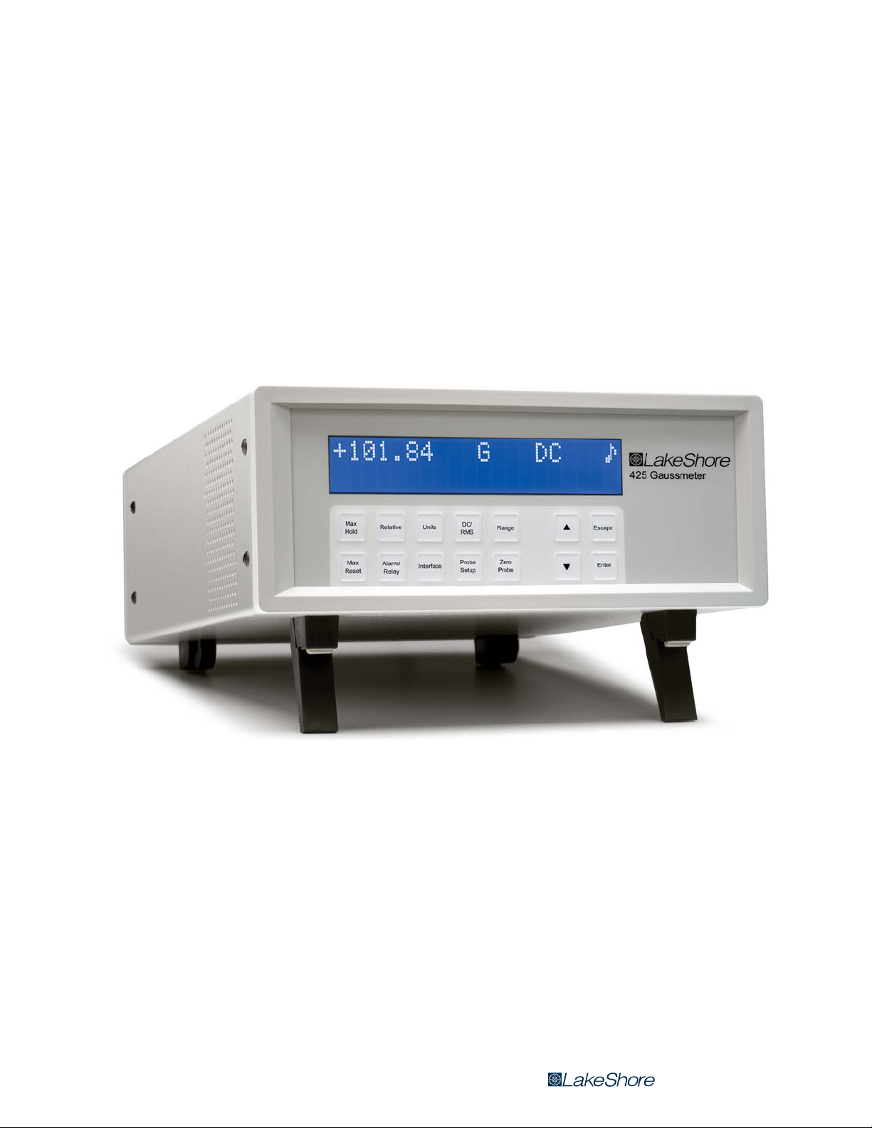
FIGURE 1-1 Model 425 front view
1.1 Product Description
Features:
D Field ranges from 350 mG to 350 kG
D DC measurement resolution to 43/e digits (1 part of ±35,000)
D Basic DC accuracy of ±0.20%
D DC to 10 kHz AC frequency
D USB interface
D Large liquid crystal display
D Sort function (displays pass/fail message)
D Alarm with relay
D Standard probe included
D Standard and custom probes available
Designed to meet the demanding needs of the permanent magnet industry, the
Lake Shore Model 425 gaussmeter provides high end functionality and performance
in an affordable desktop instrument. Magnet testing and sorting have never been
easier. When used in combination with the built in relay and audible alarm features,
the Model 425 takes the guesswork out of pass/fail criteria. Additional features
including DC to 10 kHz AC frequency response, max hold and relative measurement
make the Model 425 the ideal tool for your manufacturing, quality control and R&D
flux density measurement applications. For added functionality and value, the
Model 425 also includes a standard Lake Shore Hall probe. Put the Model 425 gaussmeter to use with confidence knowing it’s supported by the industry leading experts
in magnet measurement instrument, sensor and Hall probe technology.
1.1.1 Throughput
Throughput involves much more than just the update rate of an instrument. An intuitive menu navigation and keypad, along with overall ease of use are equally important. The Model 425 is designed with these qualities in mind. The operation is
straightforward, with user display prompts to aid set-up. We understand that time is
money! In addition to being user friendly, the automated magnet testing and sorting
features of the Model 425 streamline sorting and testing operations. In addition, hot
swapping of Hall probes allows you to switch probe types without powering the
instrument off and back on. These features support increased productivity, allowing
you to spend less time setting up your instrument and more time working on the task
at hand.
| www.lakeshore.com

2 cHAPTER 1: Introduction
1.1.2 DC Measurement Mode
1.1.3 AC Measurement Mode
1.2 Measurement Features
Static or slowly changing fields are measured in DC mode. In this mode, the
Model 425 uses probe field compensation to correct for probe nonlinearities, resulting in a DC accuracy to ±0.20%. Measurement resolution is enhanced with internal
filtering, allowing resolution to 4¾ digits with reading rates to 30 readings per second over the USB interface.
In addition to the DC measurement mode, the Model 425 offers an AC measurement
mode for measuring periodic AC fields. The instrument provides an overall frequency
range of 10 Hz to 10 kHz and is equipped with both narrow and wide band frequency
modes. While in narrow band mode, frequencies above 400 Hz are filtered out for
improved measurement performance.
The Model 425 offers a variety of features to enhance the usability and convenience
of the gaussmeter.
Autorange: in addition to manual range selection, the instrument automatically
chooses an appropriate range for the measured field. Autorange works in DC and AC
measurement modes.
Probe zero: allows you to zero all ranges while in DC mode with the simple push
of a key.
Display units: field magnitude can be displayed in units of G, T, Oe, and A/m with
resistance in ).
Max hold: the instrument stores and displays the captured maximum DC or AC
field reading.
1.3 Instrument Probe Features
1.3.1 Probe Field Compensation
1.3.2 Probe Information
Relative reading: the relative mode calculates the difference between a live reading
and the relative setpoint to highlight deviation from a known field point. This feature
can be used in DC or AC measurement modes.
Instrument calibration: Lake Shore recommends an annual recalibration schedule
for all precision gaussmeters. Recalibrations are always available from Lake Shore,
but the Model 425 allows you to field calibrate the instrument if necessary. Recalibration requires a computer interface and precision low resistance standards of known
value.
The Model 425 offers the best measurement performance when used along with
Lake Shore Hall probes. Firmware-based features work in tandem with the probe’s
calibration and programming to ensure accurate, repeatable measurements and
ease of setup. Many of the features require probe characteristics that are stored in the
probe connector’s non-volatile memory.
The Hall effect devices used in gaussmeter probes produce a near linear response in
the presence of a magnetic field. The small nonlinearities present in each individual
device can be measured and subtracted from the field reading. Model 425 probes are
calibrated in a way to provide the most accurate DC readings.
The gaussmeter reads the probe information on power up or any time the probe is
changed to allow hot swapping of probes. Critical probe information can be viewed
on the front panel and read over the computer interface to ensure proper system configuration.
1.3.3 The Probe Connection
Model 425 Gaussmeter
The Model 425 is only half the magnetic measurement equation. For the complete
solution, Lake Shore offers a full complement of standard and custom Hall effect
probes in a variety of sizes and sensitivities. One of ten standard Hall probes is
included with the Model 425. Refer to page 5 for details on the Hall probes you can
choose to receive with the Model 425.
1.3.4 Extension Ca ble 3
1.3.4 Extension Cable
1.3.5 Hall Effect Generators (Magnetic Field Sensors)
1.4 Display and Interface Features
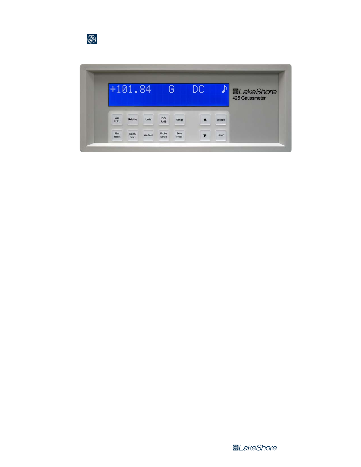
FIGURE 1-2 Left: Normal reading—the default mode with the display of the live DC field reading;
Right: Max DC hold on—the maximum value is shown in the lower display while the upper display contains the live DC field reading;
The complex nature of Hall effect measurements makes it necessary to match extension cables to the probe when longer cables are needed. Keeping probes and their
extensions from getting mixed up can become a problem when more than one probe
is used. The Model 425 alleviates most of the hassle by allowing you to match probes
to extension cables in the field. Stored information can be viewed on the front panel
and read over the computer interface to ensure proper mating.
The Model 425 will operate with a discrete Hall effect generator when a suitable
probe is not available. You can program the nominal sensitivity and serial number
into an optional HMCBL blank connector to provide all gaussmeter functions except
field compensation. If no sensitivity information is available, the Model 425 reverts to
resistance measurement.
The Model 425 has a 2-line by 20-character liquid crystal display. During normal
operation, the display is used to report field readings and give results of other features such as max or relative. When setting the instrument parameters, the display
gives you meaningful prompts and feedback to simplify operation.
Following are four examples of the various display configurations:
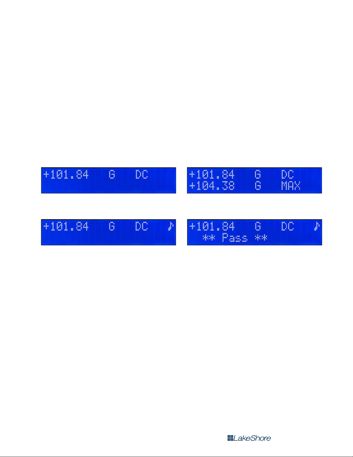
FIGURE 1-3 Left: Alarm on—the alarm gives an audible and visual indication of when the field value is selectively outside or inside a user
specified range; The relay can be associated with the alarm;
Right: Sort on—the live reading is shown in the upper display while the lower display contains the pass/fail (repetitive sorting or testing)
message. The relay facilitates pass/fail operation
1.4.1 Keypad
1.4.2 Alarm, Relay and Sort
1.4.3 Monitor Output
The instrument keypad has 14 keys with individual keys assigned to frequently used
features. Menus are reserved for less frequently used setup operations. The keypad
can be locked out to prevent unintended changes of instrument setup.
High and low alarm functions and one relay are included with the instrument, and
can be used to automate repetitive magnet testing and sorting operations. Alarm
actuators include display annunciator, audible beeper, and a relay. The alarm can be
configured to display a pass or fail message and the relay can be configured to activate a mechanism to separate parts that meet pre-set fail criteria. The relay can also
be controlled manually for other system needs.
The monitor output provides an analog representation of the reading that is corrected for probe offset and nominal sensitivity. This feature makes it possible to view
the analog signal, which has not been digitally processed. The monitor output can be
connected to an oscilloscope or data acquisition system.
| www.lakeshore.com
4 cHAPTER 1: Introduction
1.4.4 Computer Interface
1.4.5 Model 425 Rear Panel
1.5 Hall Probe Selection
The Model 425 is equipped with a universal serial bus (USB) interface. It emulates an
RS-232C serial port at a fixed baud rate of 57,600, but with the physical connections
of a USB. In addition to gathering data, nearly every function of the instrument can be
controlled through the USB interface. The reading rate over the interface is nominally
30 readings per second. A LabVIEW™ driver is available from the download section of
the Lake Shore website at www.lakeshore.com.
FIGURE 1-4 Model 425 rear panel showing the line input assembly,
USB interface, auxiliary I/O and the probe input
Listed below are the probes that you can choose from to include with your Model 425.
Our experts can guide you through the probe selection process. Other standard
probes are available at an additional cost. Lake Shore prides itself on making every
attempt to satisfy customer requests for special probes. If you need a custom probe,
contact Lake Shore for availability.
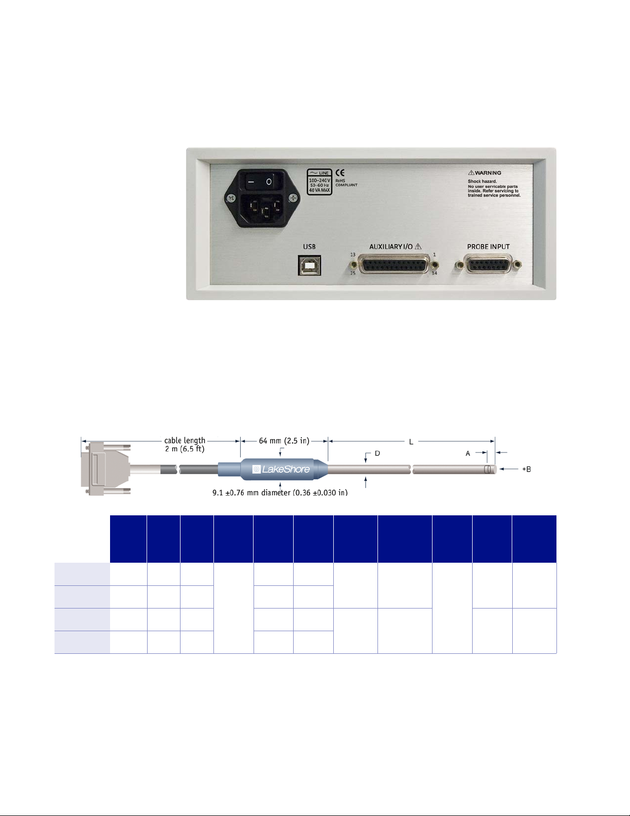
1.5.1 Axial Probes
L (in) D (in) A (in)
HMNA-1904-VR 4 ±0.125
HMMA-2502-VR 2 ±0.063
HMNA-1904-VF 4 ±0.125
HMMA-2502-VF 2 ±0.063
0.187 dia
±0.005
0.25 dia
±0.006
0.187 dia
±0.005
0.25 dia
±0.006
0.005
±0.003
0.015
±0.005
0.005
±0.003
0.015
±0.005
Active area
(in)
0.030 dia
(approx)
FIGURE 1-5 Axial probe
Stem
material
Fiberglass
epoxy
Aluminum
Fiberglass
epoxy
Aluminum
Frequency
range
DC to
10 kHz
DC to
10 kHz
DC to
800 Hz
DC to
400 Hz
TABLE 1-1 Axial probe
Usable full
scale ranges
HSE
35 G 350 G,
3.5 kG, 35 kG
HST-4
350 G, 3.5 kG,
35 kG
Corrected
accuracy
(% rdg)
±0.20% to 30 kG
and ±0.25% 30
to 35 kG
±0.10% to 30 kG
and ±0.15% 30
to 35 kG
Operating
temp
range
0 °C to
+75 °C
Tem p
coefficient
(max) zero
±0.09 G/°C -0.04%/°C
±0.13 G/°C -0.005%/°C
Tem p
coefficient
(max)
calibration
Model 425 Gaussmeter
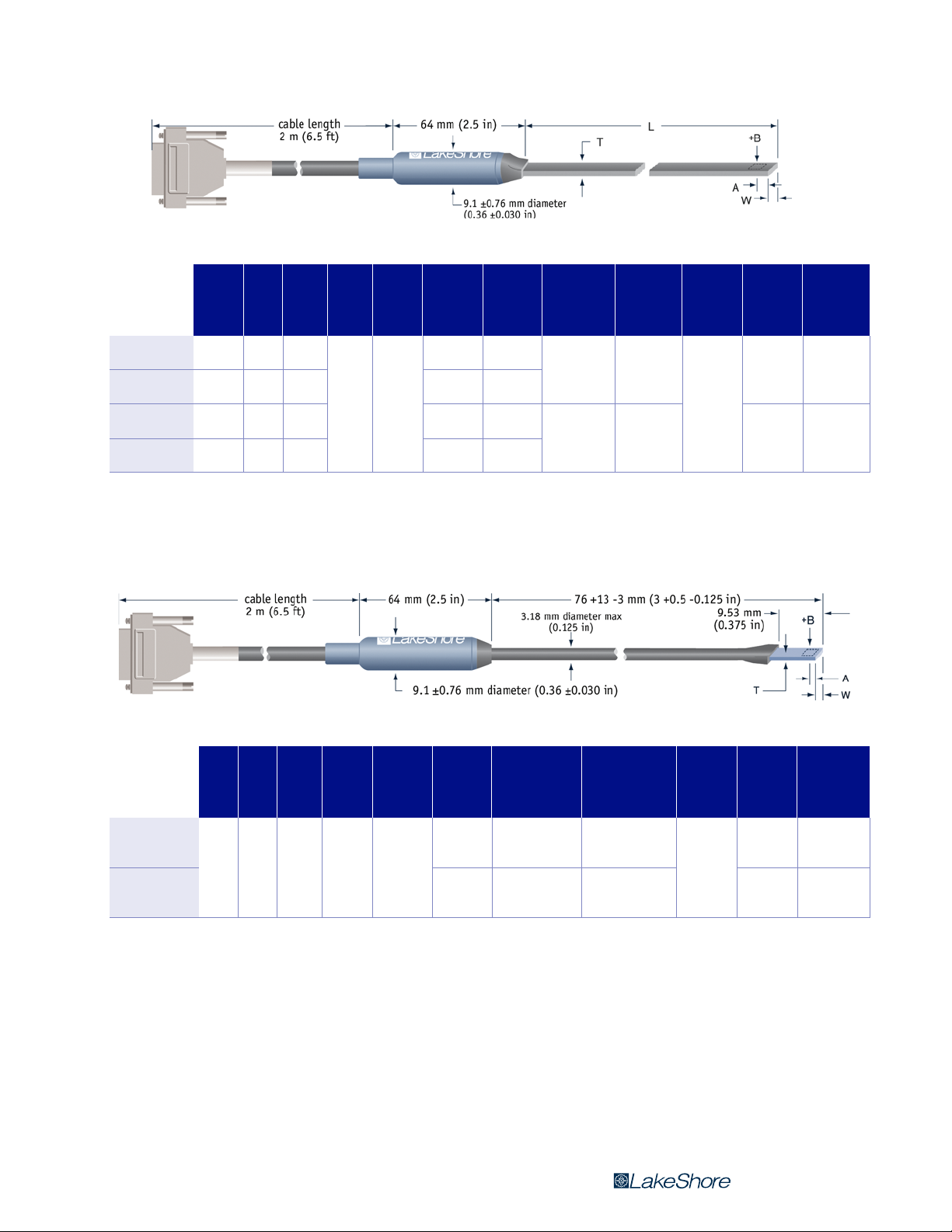
1.5.2 Transverse Probes
1.5.2 Transverse Pr obes 5
FIGURE 1-6 Transv ers e prob e
L (in) T (in) W (in) A (in)
HMMT-6J04-VR 4 ±0.125
HMNT-4E04-VR 4 ±0.125
HMMT-6J04-VF 4 ±0.125
HMNT-4E04-VF 4 ±0.125
1.5.3 Flexible Transverse Probes
0.061
max
0.045
max
0.061
max
0.045
max
0.180
±0.005
0.150
±0.005
0.180
±0.005
0.150
±0.005
0.150
±0.050
Active
area (in)
0.040 dia
(approx)
Stem
material
Aluminum
Fiberglass
epoxy
Aluminum
Fiberglass
epoxy
Frequency
range
DC to
800 Hz
DC to
10 kHz
DC to
400 Hz
DC to
800 Hz
TABLE 1-2 Transverse probe
FIGURE 1-7 Flexible transverse probe
Usable f ull
scale ranges
HSE
35 G, 350 G,
3.5 kG, 35 kG
HST-4
350 G, 3.5 kG,
35 kG
Corrected
accuracy
(% rdg)
±0.20% to
30 kG;
±0.25%
30 to 35 kG
±0.10% to
30 kG;
±0.15%
30 to 35 kG
Operating
temp
range
0 °C to
+75 °C
Te m p
coefficient
(max) zero
±0.09 G/°C -0.04%/°C
±0.13 G/°C -0.005%/°C
Tem p
coefficient
(max)
calibration
Operating
temp
range
0 °C to
+75 °C
HMFT-3E03-VR
HMFT-3E03-VF
W (in) T (in) A (in)
0.135
0.025
0.125
max
max
±0.005
Active
area (in)
0.040 dia
(approx)
Stem
material
Flexible
plastic
tubing
Frequency
range
DC to
10 kHz
DC to
800 Hz
Usable f ull
scale ranges
HSE
35 G, 350 G,
3.5 kG, 35 kG
HST-4
350 G, 3.5 kG,
35 kG
Corrected
accuracy (% rdg )
±0.20% to 30 kG;
±0.25% 30 to 35 kG
±0.10% to 30 kG;
±0.15% 30 to 35 kG
TABLE 1-3 Flexible transverse probe
Te m p
coefficient
(max) zero
±0.09 G/°C -0.04%/°C
±0.13 G/°C -0.0 05%/°C
Tem p
coefficient
(max)
calibration
| www.lakeshore.com
6 cHAPTER 1: Introduction
1.6 Model 425 Specifications
1.6.1 General Measurement
1.6.2 DC Measurement
(Does not include probe error, unless otherwise specified)
Input type: Single Hall effect sensor
Maximum update rate: 30 rdg/s
Probe features: Linearity compensation, probe zero, and hot swap
Measurement features: Autorange, max hold, relative mode, and filter
Probe connector: 15-pin D-sub socket
Probe type
Range
HST Probe
350 kG 000.01 kG 000.1 kG
35 kG 00.001 kG 00.01 kG
3.5 kG 0.0001 kG 0.001 kG
350 G 000.02 G 000.1 G
HSE Probe
35 kG 00.001 kG 00.01 kG
3.5 kG 0.0001 kG 0.001 kG
350 G 000.01 G 000.1 G
35 G 00.001 G 00.01 G
UHS Probe
35 G 00.001 G 00.01 G
3.5 G 0.0001 G 0.001 G
350 mG 000.02 mG 000.1 mG
TABLE 1- 4 DC measurement resolution
Filter on
4 r-digit resolution
Filter off
3 r-digit resolution
Measurement resolution (RMS noise floor): Indicated by value in above table for
shorted input
Display resolution: Indicated by number of digits in above table
DC accuracy: ±0.20% of reading ±0.05% of range
DC temperature coefficient: -0.01% of reading -0.003% of range/°C
DC filter: 16-point moving average
1.6.3 AC Measurement
Model 425 Gaussmeter
Probe type
Ranges
HST Probe
350 kG 000.1 kG
35 kG 00.01 kG
3.5 kG 0.001 kG
350 G 000.1 G
HSE Probe
35 kG 00.01 kG
3.5 kG 0.001 kG
350 G 000.1 G
35 G 00.01 G
UHS Probe
35 G 00.01 G
3.5 G 0.001 G
350 mG 000.1 mG
3r-digit re solution
TABLE 1-5 AC measurement resolution
Measurement resolution (RMS noise floor): Indicated by value in above table, measured at mid-scale range
Display resolution: Indicated by number of digits in above table

1.6.4 Front Panel 7
Narrow band mode Wide band mode
±2% of reading, ±0.05% of range
AC accuracy
AC frequency response 10 Hz to 400 Hz 50 Hz to 10 kHz
Minimum input signal >1% of range
AC specifications based on sine wave inputs or signals with crest factors <4.
(20 Hz to 100 Hz);
±2.5% of reading, ±0.05% of range
(10 Hz to 400 Hz)
TABLE 1-6 AC specifications
±2% of reading, ±0.05% of
range (50 H z to 10 kHz)
>1% of range, except >2% of
range on lo west range
AC temperature coefficient: ±0.01% of reading ±0.006% of range/°C
1.6.4 Front Panel
1.6.5 Interfaces
Display: 2-line × 20-character LCD display module with 5.5 mm high characters and
LED backlight
Display units: Gauss (G), tesla (T), oersted (Oe), and ampere per meter (A/m)
Display update rate: 3 rdg/s
Display resolution: To ± 4r
digits
Units multipliers: µ, m, k, M
Display annunciations: DC—DC measurement mode; RMS—AC RMS measurement
mode; MAX—Max hold value;ª
— Alarm on
Keypad: 14-key membrane
Front panel features: Display contrast control and keypad lock-out
USB
Function: Emulates a standard RS-232 serial port
Baud rate: 57,600
Connector: B-type USB connector
Reading rate: To 30 rdg/s
Software support: LabVIEW™ driver (consult Lake Shore for availability)
Alarm
Settings: High setpoint, low setpoint, inside or outside, algebraic or magnitude, audible on/off, and sort
Actuators: Display annunciator, sort message, beeper, and relay
Relay
Number: 1
Contacts: Normally open (NO), normally closed (NC), and common (C)
Contact rating: 30 VDC at 2 A
Operation: Follows alarm or operated manually
Connector: Shared 25-pin D-sub socket
Monitor output
Configuration: Real time analog voltage output proportional to measured field
Range: ±3.5 V
Scale: ±3.5 V = ±full scale on selected range
Frequency response: DC to 10 kHz
Accuracy: Offset and single point gain corrected to ±0.5% of reading ±0.1% of range,
linearity is probe dependent
Minimum load resistance: 1 k) (short circuit protected)
Connector: Shared 25-pin D-sub socket
| www.lakeshore.com

8 cHAPTER 1: Introduction
1.6.6 General
1.6.7 Probes and Extensions
1.7 Ordering Information
The Model 425 is the replacement for the Model 421 with a new software
command set.
Ambient temperature: 15 °C to 35 °C at rated accuracy; 5 °C to 40 °C with reduced
accuracy
Ambient field: Up to 100 G DC, measured at the instrument chassis
Power requirement: 100 VAC to 240 VAC, 50 Hz or 60 Hz 40 VA
Size: 216 mm W × 89 mm H × 318 mm D (8.5 in × 3.5 in ×12.5 in), half rack
Weight: 2.1 kg (4.6 lb)
Approval: CE mark, RoHS compliant
Probe compatibility: Full line of standard and custom probes (compatible with
Model 425/455/475 probes)
Hall sensor compatibility: Front panel programmable sensitivity and serial number
for user supplied Hall sensor using HMCBL cable
Extension cable compatibility: Calibrated or uncalibrated probe extension cables
with an EEPROM are available from 10 ft to 100 ft
Part number Descrip tion
425 Model 425 gaussmeter
425-HMXX-XXXX-XX
Specify power cord option
VAC-120 Instrument shipped with U.S. power cord for 120 VAC
VAC-220 Instrument shipped with European power cord for 220 VAC
VAC-120-ALL Instrument shipped with U.S. power cord (120 VAC) and European power cord (220 VAC)
Accessories included
G-106-253 I/O mating plug
G-106-264 I/O mating connector shell
4060 Zero g auss ch amber
MAN-425 Model 425 user manual
Accessories available
4065 Large zero gauss chamber for gamma probe
HMCBL-6 User programmable cable with EEPROM (6 ft)
HMCBL-20 User programmable cable with EEPROM (20 ft)
HMPEC-10-U Probe extension cable with EEPROM (10 ft), uncalibrated
HMPEC-25-U Probe extension cable with EEPROM (25 ft), uncalibrated
HMPEC-50-U Probe extension cable with EEPROM (50 ft), uncalibrated
HMPEC-100-U Probe extension cable with EEPROM (100 ft), uncalibrated
RM-q Rack mount kit for one q-rack gaussmeter in 483 mm (19 in) rack
RM-2 Rack mount kit for two q-rack gaussmeter in 483 mm (1 9 in) rack
4030-12 Hall probe stand; 305 mm (12 in) post
4030-24 Hall probe stand; 610 mm (24 in) post
Calibration service
CAL-N7-DATA New instrument calibration for Model 425/455/475 with certificate and data
CAL-425-CERT Instrument recalibration with certificate
CAL-425-DATA Instrument recalibration with certificate and data
One probe included (additional probes ordered separately)
Custom probes available—consult Lake Shore
Model 425 gaussmeter with standard probe choice—specify selected probe number for
HMXX-XXXX-XX (see list in section 1.5)
TABLE 1-7 Ordering information
Model 425 Gaussmeter

1.8 Safety Summary and Symbols 9
1.8 Safety Summary and Symbols
Observe these general safety precautions during all phases of instrument operation,
service, and repair. Failure to comply with these precautions or with specific warnings elsewhere in this manual violates safety standards of design, manufacture, and
intended instrument use. Lake Shore Cryotronics, Inc. assumes no liability for user
failure to comply with these requirements.
The Model 425 protects the operator and surrounding area from electric shock or
burn, mechanical hazards, excessive temperature, and spread of fire from the instrument. Environmental conditions outside of the conditions below may pose a hazard
to the operator and surrounding area.
D Indoor use
D Altitude to 2000 m
D Temperature for safe operation: 5 °C to 40 °C
D Maximum relative humidity: 80% for temperature up to 31 °C decreasing
linearly to 50% at 40 °C
D Environments with conducted RF of 1 V
in field readings up to 10% and monitor output up to 5%
D Power supply voltage fluctuations not to exceed ±10% of the nominal voltage
D Overvoltage category II
D Pollution degree 2
Ground the Instrument
To minimize shock hazard, the instrument is equipped with a 3-conductor AC power
cable. Plug the power cable into an approved 3-contact electrical outlet or use a
3-contact adapter with the grounding wire (green) firmly connected to an electrical
ground (safety ground) at the power outlet. The power jack and mating plug of the
power cable meet Underwriters Laboratories (UL) and International Electrotechnical
Commission (IEC) safety standards.
or EM fields of 1 V/m can cause a shift
rms
Ventilation
The instrument has ventilation holes in its side covers. Do not block these holes when
the instrument is operating.
Do Not Operate in an Explosive Atmosphere
Do not operate the instrument in the presence of flammable gases or fumes. Operation of any electrical instrument in such an environment constitutes a definite safety
hazard.
Keep Away from Live Circuits
Operating personnel must not remove instrument covers. Refer component replacement and internal adjustments to qualified maintenance personnel. Do not replace
components with power cable connected. To avoid injuries, always disconnect power
and discharge circuits before touching them.
Do Not Substitute Parts or Modify Instrument
Do not install substitute parts or perform any unauthorized modification to the
instrument. Return the instrument to an authorized Lake Shore Cryotronics, Inc. representative for service and repair to ensure that safety features are maintained.
Cleaning
Do not submerge instrument. Clean only with a damp cloth and mild detergent. Exterior only.
| www.lakeshore.com
10 cHAPTER 1: Introduction
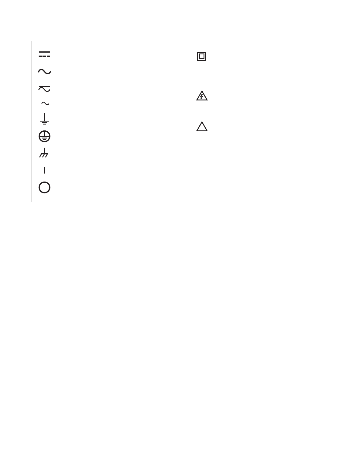
!
Direct current (power line)
Equipment protected throughout
by double insulation or reinforces
insulation (equivalent to Class II of
IEC 536—see Annex H)
CAUTION: High voltages; danger of
electric shock; background color:
yellow; symbol and outline: black
CAUTION or WARNING: See
instrument documentation;
background color: yellow;
symbol and outline: black
Off (supply)
On (supply)
Frame or chassis terminal
Protective conductor terminal
Earth (ground) terminal
3
Three-phase alternating current (power line)
Alternating or direct current (power line)
Alternating current (power line)
FIGURE 1-8 Safety symbols
Model 425 Gaussmeter
2.2.1 DC Measurem ent 11
Gain
Low pass
filter
Product
detector
RMS-to-DC
converter
Computer
interface
µPA/D
Monitor out Display
Switch
Switch
Wide band
DC or narrow band
DC
AC modes
Ic
B
Chapter 2: Background
2.1 General
2.2 Model 425 Overview
2.2.1 DC Measurement
This chapter provides background information related to the Model 425 gaussmeter.
It is intended to give insight into the benefits and limitations of the instrument and
help apply the features of the Model 425 to a variety of situations. It covers flux density, Hall measurement, and probe operation. For information on how to install the
Model 425, please refer to Chapter 3. Instrument operation information is contained
in Chapter 4 and Chapter 5.
The Model 425 gaussmeter is a highly configurable device with many built-in features. It offers a DC mode to measure static or slowly changing fields, two different
modes to measure AC fields, narrow band and wide band, and a monitor output. Refer
to section 2.2.1 and section 2.2.2 for more information on these modes. To better
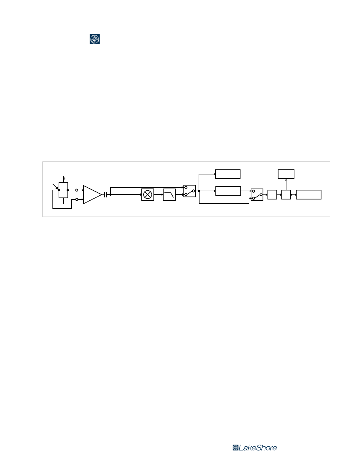
illustrate the capabilities of the gaussmeter, refer to the Model 425 system block diagram, FIGURE 2-1.
FIGURE 2-1 Model 425 system block diagram
When in DC mode, the instrument uses a 100 mA, 5.4 kHz square wave excitation current. The voltage that is generated by the Hall sensor goes through an AC coupled programmable gain stage. From there it passes through the product detector for
demodulation, a low pass filter, and the A/D converter. The digitized data is then sent
to the microprocessor. The monitor output will provide a DC voltage proportional to
the measured DC field. Refer to section 4.5.1 for the procedure to set the DC measurement mode. Refer to section 5.3 for information on monitor output.
2.2.2 AC Measurement
Narrow band mode: in this mode, the instrument uses a 100 mA, 5.4 kHz square wave
excitation current. This type of excitation provides the benefit of noise cancellation
characteristics of the product detector, but it limits the maximum field frequency of
the Model 425 to approximately 400 Hz.
The voltage that is generated by the Hall sensor goes through an AC coupled programmable gain stage. From there it passes through the product detector for demodulation, a low-pass filter, and an RMS-to-DC converter, before it is sent into the A/D
converter. The digitized data is then sent to the microprocessor. The monitor output
will provide an AC voltage proportional to the measured AC field. Refer to
section 4.5.2.1 for the procedure to set the narrow band AC measurement mode.
Wide band mode: in this mode, the instrument uses a 100 mA, DC excitation current to
drive the Hall sensor. This excitation type provides the greatest frequency range for
AC RMS measurements, up to 10 kHz. Since the signal doesn’t pass through the product detector and low pass filter, it has a higher noise floor than narrow band mode.
| www.lakeshore.com

12 cHAPTER 2: Background
φ
φ
The voltage that is generated by the Hall sensor goes through an AC coupled programmable gain stage and is sent directly to an RMS-to-DC converter. The signal is
then sent into the A/D converter. The digitized data is then sent to the microprocessor.
The monitor output will provide an unfiltered AC voltage proportional to the measured AC field. Refer to section 4.5.2.2 for the procedure to set the AC wide band
mode.
2.2.3 Monitor Output
2.3 Flux Density Overview
2.3.1 What is Flux Density?
The Model 425 has a monitor output that provides an analog representation of the
reading and is corrected for probe offset and nominal sensitivity. This monitor output
makes it possible to view the analog signal, which has not been digitized. The monitor
output can be connected to an oscilloscope or data acquisition system for analysis.
A magnetic field can be envisioned as lines of force measured in maxwells (Mx). In the
cgs system, magnetic flux ( ) is the Mx, where 1 Mx = 1 line of flux. In the SI system,
magnetic flux is the weber (Wb), where: 1 Wb = 10
Flux density is the number of flux lines passing perpendicular through a plane of unit
area (A). The symbol for flux density is B, where B = /A. The cgs system measures flux
2
density in gauss (G), where 1 G = 1 Mx/cm
tesla (T), where 1 T = 1 Wb/m
Flux density is important when magnet systems concentrate flux lines into a specific
area like the pole pieces of an electromagnet. Forces generated on current carrying
wires like those in a motor armature are proportional to flux density. Saturation of
magnetic core material is also a function of flux density.
Additional conversion factors can be found in the Appendix.
2
.
. The SI system measures flux density in
8
Mx.
2.3.2 How Flux Density (B) Differs from Magnetic Field Strength (H)
Flux density is often confused with magnetic field strength. Magnetic field strength is
a measure of the force producing flux lines. The symbol for magnetic field strength is
H. In the cgs system, it is measured in oersteds (Oe). In the SI system, it is measured in
amperes per meter (A/m):
1 Oe = 79.58 A/m
Flux density and magnetic field strength are related by the permeability (µ) of the
magnetic medium. B = µH. Permeability is a measure of how well a material makes a
path for flux lines.
The confusion of flux density and magnetic field strength is also related to permeability. In the cgs system, the permeability of air (of vacuum) is 1. Therefore, 1 G = 1 Oe or
B = H in air. Many people incorrectly assume, therefore, that in the cgs system, B = H at
all times. Adding to the confusion, in the SI system, permeability of air is not 1, so B is
not equal to H even in air.
Model 425 Gaussmeter
2 . 4 . 1 A c t i v e A r e a 13
BF
F = –e (v × B)
(force on electron)
v
2.4 Hall Measurement Theory
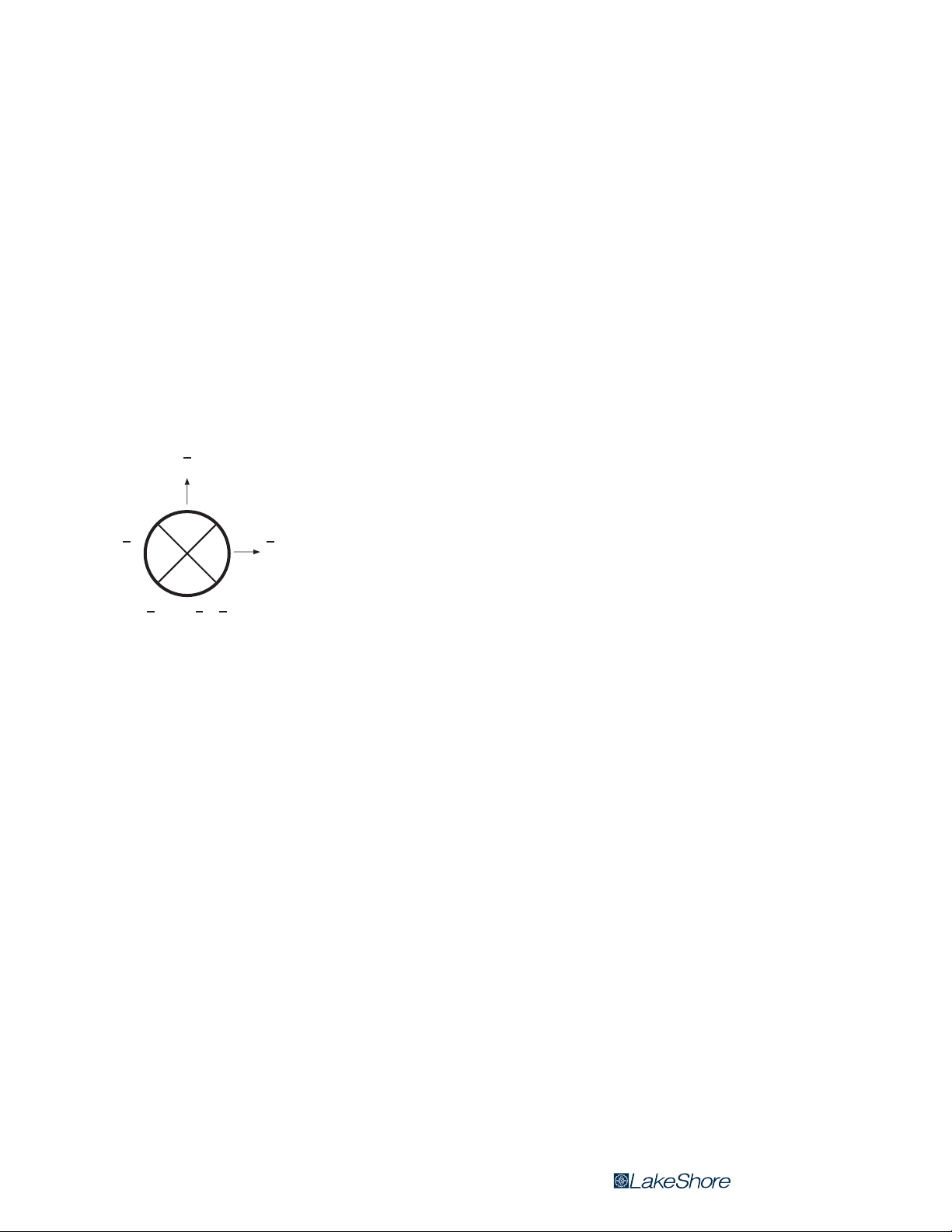
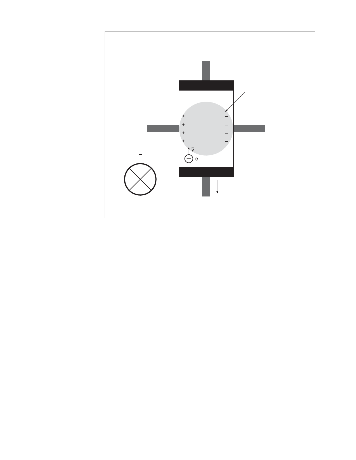
The Hall effect is the development of a voltage across a sheet of conductor when current is flowing and the conductor is placed in a magnetic field (FIGURE 2-2).
The Hall effect was discovered by E. H. Hall in 1879 and it remained a laboratory curiosity for nearly 70 years. Finally, development of semiconductors brought Hall generators into the realm of the practical. A Hall generator is a solid state sensor with a
conductor that provides an output voltage proportional to magnetic flux density. As
implied by its name, this sensor relies on the Hall effect.
Electrons (the majority carrier most often used in practice) drift in the conductor
when under the influence of an external driving electric field. When exposed to a
magnetic field, these moving charged particles experience a force perpendicular to
both the velocity and magnetic field vectors. This force causes the charging of the
edges of the conductor, one side positive, the other side negative. This edge charging
sets up an electric field which exerts a force on the moving electrons equal and opposite to that caused by the magnetic-field-related Lorentz force. The voltage potential
across the width of the conductor is called the Hall voltage. This Hall voltage can be
used in practice by attaching two electrical contacts to each of the sides of the conductor.
The Hall voltage can be given by the expression:
V
= γ
B sin θ
H
B
where: V
= Hall voltage (mV)
H
= Magnetic sensitivity (mV/kG) (at a fixed current)
γ
B
B = Magnetic field flux density (kG)
θ = Angle between magnetic flux vector and the plane of Hall generator.
As can be seen from the formula above, the Hall voltage varies with the angle of the
sensed magnetic field, reaching a maximum when the field is perpendicular to the
plane of the Hall generator.
2.4.1 Active Area The Hall generator assembly contains the semiconductor material to which the four
contacts are made. This entity is normally called a Hall plate. In its simplest form, the
Hall plate is a conductor, rectangular in shape, and of fixed length, width, and thickness. Due to the shorting effect of the current supply contacts, most of the sensitivity
to magnetic fields is contained in an area approximated by a circle, centered on the
Hall plate, the diameter of which is equal to the plate width. This circle is considered
an approximation of the active area. FIGURE 2-2 illustrates an image of the approximate active area.
| www.lakeshore.com
14 cHAPTER 2: Background
VH (+) VH (–)
Approximate
active area
B
IC (+)
I
C
(–)
FIGURE 2-2 Approximate active area
2.4.2 Temperature Coefficients
There are two technically different temperature coefficients that always affect a
gaussmeter probe: the temperature coefficient of zero and the temperature coeffecient of sensitivity (section 2.4.2.1 and section 2.4.2.2). Under normal usage (reading a magnetic field), it is virtually impossible to separate the effect of each.
The Model 425 gaussmeter does not possess circuitry to allow compensation for
these temperature errors. Thus, a user operating a probe in a variable temperature
environment must be aware that both errors exist and what the maximum effect
could be. The temperature coefficients are repeatable for an individual probe. A user
can pre-measure the changes and manually correct the data for zero and sensitivity
effects, or the combination of both at specific magnetic field values. The Model 425
gaussmeter also has its own temperature coefficients, which are typically less than
probe coefficients. These are listed in section 1.6.
2.4.2.1 The Temperature Coefficient of Zero
The temperature coefficient of zero is a change in the zero field offset with temperature. This change is always present whether or not a field is measured. However, the
temperature error caused by zero change is often the dominant source of error at
magnetic field levels <100 G. If you have the ability to zero the gaussmeter at operating temperature, this coefficient is nullified and has no effect on accuracy. If the
gaussmeter cannot be zeroed, then the zero change effect is present.
Model 425 Gaussmeter
The unit of measure is G/° C. It is generally a fixed number, and can be either a positive
or negative value. This error is specific to each probe and can be a fixed magnitude
anywhere from the negative maximum to positive maximum value.

2.4.3 Radiation 15
Example of zero error: assume that the Model 425 is zeroed at +25 °C and then the temperature rises to +50 °C (,T = +25 °C). For an HMMT-6J04-VR, the worst-case zero
drift would be ±0.09 G/°C × 25 °C = ±2.25 G (maximum).
This is the maximum temperature error to be expected. Most Lake Shore probes exhibit
lower temperature coefficients.
2.4.2.2 The Temperature Coefficient of Sensitivity (Calibration)
The temperature coefficient of sensitivity is related to a change in the magnetic sensitivity of the Hall device with temperature. This change is present only when a field is
measured. The larger the field, the greater the error in G for the same temperature
change.
This characteristic is present in all probes and is specified in units of %G/° C. The
intrinsic value is always negative for Lake Shore HSE and HST probes, meaning that
the sensitivity of the Hall sensor decreases with increased temperature. Therefore,
the reading will be lower than the actual magnetic field when the probe is at a temperature higher than room temperature. Lake Shore Hall probes are calibrated at
room temperature (25 °C); when they are used in temperatures other than this, temperature coefficient becomes another source of error. Lake Shore HST probes normally exhibit a temperature coefficient of sensitivity about ten times better (lower)
than the HSE probes.
2.4.3 Radiation
Simply handling the probe at the stem can cause sufficient temperature change of the
sensor, which can cause the reading to drift; handling the probe by the stem is not recommended as it can break the probe.
Examples of sensitivity error: assume that the Model 425 is zeroed at +25 °C and then
the temperature rises to +50 °C (Delta T = +25 °C). For an HMMT-6J04-VR and
Model 425 (no compensation), measuring a 1.000 kG field, the worst-case sensitivity
change would be -0.04%/°C × 25 °C = -1% (maximum); -1% of 1.000 kG = -10 G
(reads low 10 G).
Also note that if the probe were a Model HMMT-6J04-VF, the worst case sensitivity
change would be -0.005%/°C × 25 °C = -0.125% (maximum); -0.125% of 1.000 kG =
-1.25 G (reads low 1.25 G).
This is the maximum temperature error to be expected. Most Lake Shore probes exhibit
lower temperature coefficients.
The HST and HSE probes use a highly doped indium arsenide conductor. The HST
material is the more highly doped of the two and therefore will be less affected by
radiation. Some general information relating to highly doped indium arsenide Hall
generators is provided in the following list. The changes in sensitivity are the maximums expected if the sensor is exposed at the given rates indefinitely.
D Gamma radiation seems to have little effect on the Hall generators
D Proton radiation up to 10 Mrad causes sensitivity changes less than 0.5%
D Neutron cumulative radiation (>0.1 MeV, 10
15
/cm2) can cause a 3% to 5%
decrease in sensitivity
In all cases the radiation effects on the Hall sensors seem to saturate and diminish
with cumulative exposure; the length of time for these effects to diminish varies
depending upon radiation intensity.
| www.lakeshore.com

16 cHAPTER 2: Background
2.5 Probe Considerations
2.5.1 Orientation
This section defines and discusses things to consider when selecting a probe.
Because accessing the field is part of the challenge when selecting a probe, field orientation dictates the most basic probe geometry choice of transverse versus axial.
Other variations are also available for less common, more challenging applications.
Listed below are the standard configurations for HSE and HST probes; UHS probes
require special construction that is not described here.
D Tra ns ver se : most often rectangular in shape, transverse probes measure fields per-
pindicular to their stem width. They are useful for most general purpose field
measurements and are essential for work in magnet gaps. Several stem lengths
and thicknesses are available as standard probes.
D Axial: usually round, axial probes measure fields perpindicular to their end. They
can also be used for general-purpose measurements, but are most commonly
used to measure fields produced by solenoids. Several stem lengths and diameters are available as standard probes.
D Flexible: with a flexible portion in the middle of their stem, flexible probes have an
active area at the tip that remains rigid and somewhat exposed. This unique feature makes them significantly more fragile than other transverse probes. Flexible
probes should only be selected for narrow-gap measurement applications.
D Ta ng en ti a l: these probes are transverse probes designed to measure fields parallel
to and near a surface. The active area is very close to the stem tip. These probes
are intended for this specific application and should not be selected for general
transverse measurements.
2.5.2 Frequency
Flexible and tangential probes are significantly more fragile than other transverse
probes.
D Multiple axis: multi-axis probes are available for multi-axis gaussmeters like the
Lake Shore Model 460. These probes are not compatible with the Model 425.
Hall effect gaussmeters are equally well suited for measuring either static, DC fields
or periodic, AC fields, but proper probe selection is required to achieve optimal
performance. HST probes are not recommended for use in wide band mode because
of their lower sensitivity. These probes perform better with the the noise cancellation
benefits of the narrow band mode.
D Metal stem: these probe stems are the best choice for DC and low frequency AC
measurements. Non-ferrous metals are used for probe stems because they
provide the best protection for the delicate Hall effect sensor without altering
the measured field. Aluminum is the most common metal stem material, but
brass can also be used. Metal stems do have one drawback: eddy currents are
generated in them when they are placed in AC fields. These eddy currents oppose
the field and cause measurement error. The error magnitude is proportional to
frequency, and is most noticeable above 800 Hz.
D Non-metal stem: these probe stems are required for higher frequency AC fields and
for measuring pulse fields—fiberglass/epoxy is a common non-metal stem
material. Alternatively, the Hall effect sensor can be left exposed on its ceramic
substrate, but provides less protection for the sensor. Eddy currents do not limit
the frequency range of these non-conductive materials, but other factors may.
Model 425 Gaussmeter
None of these probe types are suitable for direct exposure to high voltage. The possibility
exists for damage to equipment or injury to the operator if the probe is exposed to high
voltage.
 Loading...