

Page 1
User’s Manual
Model 340
Temperature Controller
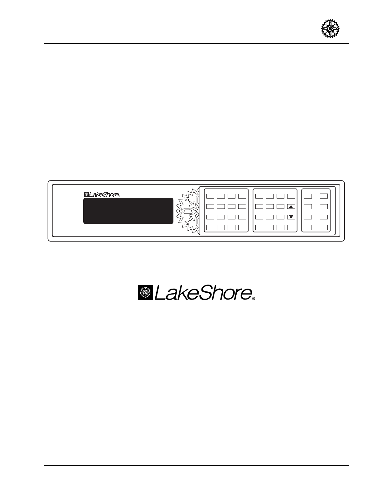
340 Temperature Controller
Auto
Zone
Tune
Settings
P I D
Heater
Control
Range
Channel
Heater
Off Setpoint
Ramp Program
Control
Setup
Loop 1
Manual
Output Loop 2
Input
Setup
7
Scan
Setup
4
Alarm
Setup
1
Alarm
Reset
0
Display
SoftCal
Format
8
Curve
Entry5Interface
Math
Analog
Setup
Outputs
2
Math
Reset.Options
Cancel
Escape
Enter
Screen More
Previous
Setting Local
Next
Setting DataCard
Save
Screen Help
9
6
3
+/-
Lake Shore Cryotronics, Inc.
575 McCorkle Blvd.
Westerville, Ohio 43082-8888 USA
Internet Addresses:
Visit Our Website:
www.lakeshore.com
Fax: (614) 891-1392
Telephone: (614) 891-2243
Methods and apparatus disclosed and described herein have been developed solely on company funds of Lake Shore Cryotronics, Inc.
No government or other contractual support or relationship whatsoever has existed which in any way affects or mitigates proprietary
rights of Lake Shore Cryotronics, Inc. in these developments. Methods and apparatus disclosed herein may be subject to U.S. Patents
existing or applied for. Lake Shore Cryotronics, Inc. reserves the right to add, improve, modify, or withdraw functions, design
modifications, or products at any time without notice. Lake Shore shall not be liable for errors contained herein or for incidental or
consequential damages in connection with furnishing, performance, or use of this material.
Rev. 2.1 P/N 119-011 29 March 2004
Page 2

Lake Shore Model 340 Temperature Controller User’s Manual
LIMITED WARRANTY STATEMENT
WARRANTY PERIOD: ONE (1) YEAR
1. Lake Shore warrants that this Lake Shore product (the “Product”) will
be free from defects in materials and workmanship for the Warranty
Period specified above (the “Warranty Period”). If Lake Shore receives
notice of any such defects during the Warranty Period and the Product
is shipped freight prepaid, Lake Shore will, at its option, either repair
or replace the Product if it is so defective without charge to the owner
for parts, service labor or associated customary return shipping cost.
Any such replacement for the Product may be either new or equivalent
in performance to new. Replacement or repaired parts will be
warranted for only the unexpired portion of the original warranty or
90 days (whichever is greater).
2. Lake Shore warrants the Product only if it has been sold by an
authorized Lake Shore employee, sales representative, dealer or
original equipment manufacturer (OEM).
3. The Product may contain remanufactured parts equivalent to new in
performance or may have been subject to incidental use.
4. The Warranty Period begins on the date of delivery of the Product or
later on the date of installation of the Product if the Product is installed
by Lake Shore, provided that if you schedule or delay the Lake Shore
installation for more than 30 days after delivery the Warranty Period
begins on the 31st day after delivery.
5. This limited warranty does not apply to defects in the Product
resulting from (a) improper or inadequate maintenance, repair or
calibration, (b) fuses, software and non-rechargeable batteries,
(c) software, interfacing, parts or other supplies not furnished by
Lake Shore, (d) unauthorized modification or misuse, (e) operation
outside of the published specifications or (f) improper site preparation
or maintenance.
6. TO THE EXTENT ALLOWED BY APPLICABLE LAW, THE
ABOVE WARRANTIES ARE EXCLUSIVE AND NO OTHER
WARRANTY OR CONDITION, WHETHER WRITTEN OR ORAL,
IS EXPRESSED OR IMPLIED. LAKE SHORE SPECIFICALLY
DISCLAIMS ANY IMPLIED WARRANTIES OR CONDITIONS OF
MERCHANTABILITY, SATISFACTORY QUALITY AND/OR
FITNESS FOR A PARTICULAR PURPOSE WITH RESPECT TO
THE PRODUCT. Some countries, states or provinces do not allow
limitations on an implied warranty, so the above limitation or
exclusion might not apply to you. This warranty gives you specific
legal rights and you might also have other rights that vary from
country to country, state to state or province to province.
7. TO THE EXTENT ALLOWED BY APPLICABLE LAW, THE
REMEDIES IN THIS WARRANTY STATEMENT ARE YOUR
SOLE AND EXCLUSIVE REMEDIES.
8. EXCEPT TO THE EXTENT PROHIBITED BY APPLICABLE
LAW, IN NO EVENT WILL LAKE SHORE OR ANY OF ITS
SUBSIDIARIES, AFFILIATES OR SUPPLIERS BE LIABLE FOR
DIRECT, SPECIAL, INCIDENTAL, CONSEQUENTIAL OR
OTHER DAMAGES (INCLUDING LOST PROFIT, LOST DATA
OR DOWNTIME COSTS) ARISING OUT OF THE USE,
INABILITY TO USE OR RESULT OF USE OF THE PRODUCT,
WHETHER BASED IN WARRANTY, CONTRACT, TORT OR
OTHER LEGAL THEORY, AND WHETHER OR NOT LAKE
SHORE HAS BEEN ADVISED OF THE POSSIBILITY OF SUCH
DAMAGES. Your use of the Product is entirely at your own risk.
Some countries, states and provinces do not allow the exclusion of
liability for incidental or consequential damages, so the above
limitation may not apply to you.
LIMITED WARRANTY STATEMENT (Continued)
9. EXCEPT TO THE EXTENT ALLOWED BY APPLICABLE LAW,
THE TERMS OF THIS LIMITED WARRANTY STATEMENT DO
NOT EXCLUDE, RESTRICT OR MODIFY, AND ARE IN
ADDITION TO, THE MANDATORY STATUTORY RIGHTS
APPLICABLE TO THE SALE OF THE PRODUCT TO YOU.
CERTIFICATION
Lake Shore certifies that this product has been inspected and tested in
accordance with its published specifications and that this product met its
published specifications at the time of shipment. The accuracy and
calibration of this product at the time of shipment are traceable to the
United States National Institute of Standards and Technology (NIST);
formerly known as the National Bureau of Standards (NBS).
FIRMWARE LIMITATIONS
Lake Shore has worked to ensure that the Model 340 firmware is as free
of errors as possible, and that the results you obtain from the instrument
are accurate and reliable. However, as with any computer-based software,
the possibility of errors exists.
In any important research, as when using any laboratory equipment,
results should be carefully examined and rechecked before final
conclusions are drawn. Neither Lake Shore nor anyone else involved in
the creation or production of this firmware can pay for loss of time,
inconvenience, loss of use of the product, or property damage caused by
this product or its failure to work, or any other incidental or consequential
damages. Use of our product implies that you understand the Lake Shore
license agreement and statement of limited warranty.
FIRMWARE LICENSE AGREEMENT
The firmware in this instrument is protected by United States copyright
law and international treaty provisions. To maintain the warranty, the
code contained in the firmware must not be modified. Any changes made
to the code is at the user’s risk. Lake Shore will assume no responsibility
for damage or errors incurred as result of any changes made to the
firmware.
Under the terms of this agreement you may only use the Model 340
firmware as physically installed in the instrument. Archival copies are
strictly forbidden. You may not decompile, disassemble, or reverse
engineer the firmware. If you suspect there are problems with the
firmware, return the instrument to Lake Shore for repair under the terms
of the Limited Warranty specified above. Any unauthorized duplication
or use of the Model 340 firmware in whole or in part, in print, or in any
other storage and retrieval system is forbidden.
TRADEMARK ACKNOWLEDGMENT
Many manufacturers and sellers claim designations used to distinguish
their products as trademarks. Where those designations appear in this
manual and Lake Shore was aware of a trademark claim, they appear with
initial capital letters and the ™ or
Apiezon
®
is a trademark of Biddle Instruments.
®
symbol.
CalCurve™, Carbon-Glass™, Cernox™, DriftTrak™, Duo-Twist™,
Quad-Lead™, Quad-Twist™, Rox™, SoftCal™, and Thermox™ are
trademarks of Lake Shore Cryotronics, Inc.
Chromel™ and Alumel™ are trademarks of Hoskins Manufacturing
Company.
Formvar™ is a trademark of Monsanto Chemical Company.
MS-DOS
®
and Windows® are trademarks of Microsoft Corporation.
NI-488.2™ is a trademark of National Instruments.
PC, XT, AT, and PS-2 are trademarks of IBM.
®
is a trademark of Emerson & Cuming.
Stycast
®
Teflon
is a trademark of DuPont De Nemours.
Copyright ©1996 – 2001 and 2003 – 2004 by Lake Shore Cryotronics, Inc. All rights reserved. No portion of this
manual may be reproduced, stored in a retrieval system, or transmitted, in any form or by any means, electronic,
mechanical, photocopying, recording, or otherwise, without the express written permission of Lake Shore.
A
Page 3
Lake Shore Model 340 Temperature Controller User’s Manual
Declaration of Conformity
We: Lake Shore Cryotronics, Inc.
575 McCorkle Blvd.
Westerville, OH 43082-8888 USA
hereby declare that the equipment specified conforms to the following
Directives and Standards:
Application of Council directives: ....................... 73/23/EEC
89/336/EEC
Standard to which Conformity is declared:......... EN 61010-1:2001
Overvoltage II
Pollution Degree 2
EN 61326 A2:2001
Class A
Annex B
Model Number:................................................... 340
_________________________________________________ __________________________________
Signature Date
Ed Maloof
Printed Name
Vice President of Engineering
Position
B
Page 4

Lake Shore Model 340 Temperature Controller User’s Manual
This Page Intentionally Left Blank
C
Page 5

Lake Shore Model 340 Temperature Controller User’s Manual
TABLE OF CONTENTS
Chapter/Paragraph Title Page
1 INTRODUCTION .................................................................................................................................................... 1-1
1.0 GENERAL ......................................................................................................................................... 1-1
1.1 TEMPERATURE CONTROL SYSTEM ............................................................................................. 1-2
1.2 TEMPERATURE CONTROL SYSTEM WITH THE MODEL 340 ...................................................... 1-2
1.2.1 Cooling Source .............................................................................................................................. 1-2
1.2.2 Feedback ....................................................................................................................................... 1-3
1.2.3 Control Equation ............................................................................................................................ 1-3
1.2.4 Heating .......................................................................................................................................... 1-3
1.3 MODEL 340 FEATURES................................................................................................................... 1-3
1.3.1 Configurable Inputs........................................................................................................................ 1-3
1.3.2 Input Isolation................................................................................................................................. 1-4
1.3.3 Input Reading Capability................................................................................................................ 1-4
1.3.4 Temperature Response Curves and CalCurves™......................................................................... 1-5
1.3.5 SoftCal™........................................................................................................................................ 1-5
1.3.6 Configurable Heater Output ........................................................................................................... 1-5
1.3.7 Heater Output Protection ............................................................................................................... 1-5
1.3.8 Second Control Loop ..................................................................................................................... 1-5
1.3.9 AutoTune ....................................................................................................................................... 1-5
1.3.10 Setpoint Ramping and Zones......................................................................................................... 1-5
1.3.11 Internal Programming .................................................................................................................... 1-6
1.3.12 Math............................................................................................................................................... 1-6
1.3.13 Alarms, Analog Outputs, and Digital I/O ........................................................................................ 1-6
1.3.14 Memory Card ................................................................................................................................. 1-6
1.3.15 Computer Interface ........................................................................................................................ 1-6
2 COOLING SYSTEM DESIGN................................................................................................................................. 2-1
2.0 General.............................................................................................................................................. 2-1
2.1 Temperature Sensor Selection .......................................................................................................... 2-1
2.1.1 Temperature Range....................................................................................................................... 2-1
2.1.2 Sensor Sensitivity .......................................................................................................................... 2-1
2.1.3 Environmental Conditions .............................................................................................................. 2-2
2.1.4 Measurement Accuracy ................................................................................................................. 2-2
2.1.5 Sensor Package............................................................................................................................. 2-2
2.2 Calibrated Sensors ............................................................................................................................ 2-2
2.2.1 Traditional Calibration .................................................................................................................... 2-2
2.2.2 SoftCal™........................................................................................................................................ 2-3
2.2.3 Standard Curves ............................................................................................................................ 2-4
2.2.4 CalCurve™ .................................................................................................................................... 2-4
2.3 SENSOR INSTALLATION................................................................................................................. 2-4
2.3.1 Mounting Materials......................................................................................................................... 2-4
2.3.2 Sensor Location ............................................................................................................................. 2-4
2.3.3 Thermal Conductivity ..................................................................................................................... 2-5
2.3.4 Contact Area .................................................................................................................................. 2-5
2.3.5 Contact Pressure ........................................................................................................................... 2-5
2.3.6 Lead Wire....................................................................................................................................... 2-6
2.3.7 Lead Soldering............................................................................................................................... 2-6
2.3.8 Heat Sinking Leads........................................................................................................................ 2-6
2.3.9 Thermal Radiation.......................................................................................................................... 2-6
2.4 HEATER SELECTION AND INSTALLATION.................................................................................... 2-6
2.4.1 Heater Resistance and Power ....................................................................................................... 2-6
2.4.2 Heater Location.............................................................................................................................. 2-7
2.4.3 Heater Types ................................................................................................................................. 2-7
2.4.4 Heater Wiring ................................................................................................................................. 2-7
2.5 CONSIDERATIONS FOR GOOD CONTROL ................................................................................... 2-7
2.5.1 Thermal Conductivity ..................................................................................................................... 2-7
2.5.2 Thermal Lag................................................................................................................................... 2-8
2.5.3 Two-Sensor Approach ................................................................................................................... 2-8
2.5.4 Thermal Mass ................................................................................................................................ 2-8
2.5.5 System Nonlinearity ....................................................................................................................... 2-8
2.6 PID CONTROL .................................................................................................................................. 2-9
2.6.1 Proportional (P).............................................................................................................................. 2-9
Table of Contents i
Page 6

Lake Shore Model 340 Temperature Controller User’s Manual
TABLE OF CONTENTS (Continued)
Chapter/Paragraph Title Page
2.6.2 Integral (I)....................................................................................................................................... 2-9
2.6.3 Derivative (D) .................................................................................................................................2-9
2.6.4 Manual Heater Output.................................................................................................................. 2-11
2.7 MANUAL TUNING ........................................................................................................................... 2-11
2.7.1 Setting Heater Range................................................................................................................... 2-11
2.7.2 Tuning Proportional...................................................................................................................... 2-11
2.7.3 Tuning Integral ............................................................................................................................. 2-12
2.7.4 Tuning Derivative ......................................................................................................................... 2-12
2.8 AUTOTUNING................................................................................................................................. 2-13
2.9 ZONE TUNING................................................................................................................................ 2-14
3 INSTRUMENT HARDWARE INSTALLATION ....................................................................................................... 3-1
3.0 GENERAL ......................................................................................................................................... 3-1
3.1 RECEIVING THE MODEL 340 .......................................................................................................... 3-1
3.1.1 Inspection and Unpacking.............................................................................................................. 3-1
3.1.2 Repackaging For Shipment............................................................................................................ 3-1
3.1.3 Safety Summary............................................................................................................................. 3-2
3.1.4 Safety Symbols ..............................................................................................................................3-2
3.1.5 Handling Liquid Helium and Liquid Nitrogen .................................................................................. 3-3
3.2 REAR PANEL DEFINITION............................................................................................................... 3-4
3.3 LINE INPUT ASSEMBLY................................................................................................................... 3-5
3.3.1 Line Voltage and Fuse Verification................................................................................................. 3-5
3.3.2 Line Voltage Selection ...................................................................................................................3-5
3.3.3 Fuse Replacement ......................................................................................................................... 3-6
3.3.4 Power Cord ....................................................................................................................................3-6
3.3.5 Power Switch ................................................................................................................................. 3-6
3.4 STANDARD SENSOR INPUTS......................................................................................................... 3-6
3.4.1 Sensor Input Connector and Pinout ............................................................................................... 3-6
3.4.2 Sensor Lead Cable ........................................................................................................................3-7
3.4.3 Grounding and Shielding Sensor Leads......................................................................................... 3-7
3.4.4 Sensor Polarity............................................................................................................................... 3-7
3.4.5 Four-Lead Sensor Measurement ...................................................................................................3-7
3.4.6 Two-Lead Sensor Measurement.................................................................................................... 3-8
3.4.7 Lowering Measurement Noise........................................................................................................ 3-8
3.5 HEATER OUTPUT SETUP ...............................................................................................................3-8
3.5.1 Loop 1 Output ................................................................................................................................3-8
3.5.2 Heater Output Connector for Loop 1 .............................................................................................. 3-8
3.5.3 Heater Output Wiring for Loop 1 ....................................................................................................3-9
3.5.4 Heater Protection and Fuse for Loop 1 .......................................................................................... 3-9
3.5.5 Loop 1 Heater Noise ...................................................................................................................... 3-9
3.5.6 Model 3003 Heater Output Conditioner.......................................................................................... 3-9
3.5.7 Loop 2 Output ..............................................................................................................................3-10
3.5.8 Loop 2 Output Resistance............................................................................................................ 3-10
3.5.9 Loop 2 Output Connector............................................................................................................. 3-10
3.5.10 Loop 2 Heater Protection ............................................................................................................. 3-10
3.5.11 Boosting the Output Power .......................................................................................................... 3-11
3.6 ANALOG OUTPUTS........................................................................................................................ 3-11
3.7 DIGITAL I/O..................................................................................................................................... 3-12
3.8 RELAYS .......................................................................................................................................... 3-12
4 FRONT PANEL OPERATION ................................................................................................................................ 4-1
4.0 GENERAL ......................................................................................................................................... 4-1
4.1 TURNING POWER ON .....................................................................................................................4-1
4.2 DISPLAY FORMATS ......................................................................................................................... 4-1
4.2.1 Normal Display............................................................................................................................... 4-2
4.2.2 Setting Displays .............................................................................................................................4-2
4.2.3 Data Entry Displays........................................................................................................................ 4-2
4.2.4 Error Displays................................................................................................................................. 4-2
4.3 KEYPAD DESCRIPTION................................................................................................................... 4-2
4.4 KEYPAD NAVIGATION ..................................................................................................................... 4-3
4.4.1 Entering Settings............................................................................................................................ 4-3
4.4.2 Direct Settings................................................................................................................................ 4-3
ii Table of Contents
Page 7

Lake Shore Model 340 Temperature Controller User’s Manual
TABLE OF CONTENTS (Continued)
Chapter/Paragraph Title Page
4.4.3 Using Setting Screens ................................................................................................................... 4-4
4.4.4 Data Entry Screens........................................................................................................................ 4-4
4.4.5 The Help Key ................................................................................................................................. 4-4
4.4.6 Keypad Time-out............................................................................................................................ 4-4
4.4.7 Key Definitions............................................................................................................................... 4-5
4.5 CHANGING DISPLAY FORMAT ....................................................................................................... 4-6
4.5.1 Number of Readings Displayed ..................................................................................................... 4-6
4.5.2 Sensor Input................................................................................................................................... 4-6
4.5.3 Reading Source and Display Units ................................................................................................ 4-7
4.5.4 Control Loop Display...................................................................................................................... 4-7
4.5.5 Large Heater Display ..................................................................................................................... 4-7
4.5.6 Heater Output Display Units........................................................................................................... 4-8
4.5.7 Display Contrast............................................................................................................................. 4-8
4.5.8 Display Backlight On/Off ................................................................................................................ 4-8
4.5.9 Locking the Keypad ....................................................................................................................... 4-8
4.6 DEFAULT VALUES ........................................................................................................................... 4-8
5 SENSOR INPUT AND TEMPERATURE MEASUREMENT OPERATION............................................................. 5-1
5.0 GENERAL ......................................................................................................................................... 5-1
5.1 SENSOR INPUT SETUP................................................................................................................... 5-1
5.1.1 Sensor Type................................................................................................................................... 5-1
5.1.2 Voltage Excitation (Current Autorange) ......................................................................................... 5-2
5.1.3 Thermal EMF Compensation with Voltage Excitation .................................................................... 5-2
5.1.4 Special Sensor Type Configuration................................................................................................ 5-2
5.1.5 Turning an Input Off ....................................................................................................................... 5-3
5.2 SELECTING A TEMPERATURE RESPONSE CURVE .................................................................... 5-3
5.3 FILTER AND MATH .......................................................................................................................... 5-4
5.3.1 Filter............................................................................................................................................... 5-4
5.3.2 Max/Min ......................................................................................................................................... 5-5
5.3.3 Linear Equation.............................................................................................................................. 5-6
5.4 SCANNER SUPPORT....................................................................................................................... 5-6
5.4.1 Scan Modes ................................................................................................................................... 5-6
5.4.2 Input Setup with a Scan Mode Active ............................................................................................ 5-7
5.4.3 Manual Scanning ........................................................................................................................... 5-7
5.4.4 Auto Scanning................................................................................................................................ 5-8
5.4.5 Slave Scanning .............................................................................................................................. 5-8
6 TEMPERATURE CONTROL OPERATION............................................................................................................ 6-1
6.0 GENERAL ......................................................................................................................................... 6-1
6.1 CONTROL LOOPS............................................................................................................................ 6-1
6.1.1 Control Loops on the Normal Display ............................................................................................ 6-1
6.1.2 Loop Indication on the Normal Display .......................................................................................... 6-1
6.1.3 Loop Indication on Setting Screens ............................................................................................... 6-1
6.1.4 Control Output Display................................................................................................................... 6-2
6.2 CONTROL LOOP ENABLE............................................................................................................... 6-2
6.3 CONTROL LOOP FILTER................................................................................................................. 6-2
6.4 CONTROL CHANNEL....................................................................................................................... 6-3
6.5 CONTROL MODES........................................................................................................................... 6-3
6.6 MANUAL SETTING OF PID CONTROL PARAMETERS .................................................................. 6-4
6.6.1 Proportional (P).............................................................................................................................. 6-4
6.6.2 Integral (I)....................................................................................................................................... 6-4
6.6.3 Derivative (D) ................................................................................................................................. 6-4
6.6.4 Manual Output ............................................................................................................................... 6-4
6.7 SELECTING AN AUTOTUNE CONTROL MODE ............................................................................. 6-4
6.8 ZONE CONTROL DATA ENTRY ...................................................................................................... 6-5
6.9 USING OPEN LOOP CONTROL....................................................................................................... 6-7
6.10 SETTING A SETPOINT AND SETPOINT UNITS.............................................................................. 6-7
6.11 SETPOINT RAMPING....................................................................................................................... 6-8
6.12 CONTROL OUTPUT ......................................................................................................................... 6-8
6.12.1 Heater Output Parameter Settings and Heater Range................................................................... 6-8
6.12.2 Analog Output as Loop 2 Control Output ..................................................................................... 6-10
Table of Contents iii
Page 8

Lake Shore Model 340 Temperature Controller User’s Manual
TABLE OF CONTENTS (Continued)
Chapter/Paragraph Title Page
6.13 CONTROL OUTPUT LIMITS........................................................................................................... 6-11
6.13.1 Setpoint Limit ...............................................................................................................................6-11
6.13.2 Control Output Slope Limit ........................................................................................................... 6-11
6.13.3 Heater Range Limit ...................................................................................................................... 6-11
7 ANALOG OUTPUT, DIGITAL I/O. ALARMS, AND RELAY OPERATION ............................................................ 7-1
7.0 GENERAL ......................................................................................................................................... 7-1
7.1 ANALOG OUTPUTS.......................................................................................................................... 7-1
7.1.1 Input Mode for Analog Output ........................................................................................................7-2
7.1.2 Example of Low and High Parameter Setting ................................................................................7-2
7.1.3 Loop 2 Mode for Analog Output 2 ..................................................................................................7-2
7.1.4 Manual Mode Operation of the Analog Outputs ............................................................................. 7-3
7.2 DIGITAL INPUTS AND OUTPUTS (I/O)............................................................................................7-3
7.2.1 Digital Output Modes...................................................................................................................... 7-3
7.2.2 Digital Outputs in Alarm Mode ....................................................................................................... 7-3
7.2.3 Digital Outputs in Scanner Mode.................................................................................................... 7-3
7.2.4 Digital Outputs in Manual Mode ..................................................................................................... 7-4
7.2.5 Digital Input Modes ........................................................................................................................ 7-4
7.3 INPUT ALARMS ................................................................................................................................7-4
7.3.1 Enabling an Input Alarm................................................................................................................. 7-4
7.3.2 Selecting an Input Alarm Source.................................................................................................... 7-5
7.3.3 Input Alarm High and Low Settings ................................................................................................ 7-5
7.3.4 Input Alarm Latching ...................................................................................................................... 7-5
7.3.5 Input Alarm Relay Setup ................................................................................................................ 7-5
7.3.6 Input Alarm Reset ..........................................................................................................................7-6
7.3.7 Audible Beeper............................................................................................................................... 7-6
7.4 HIGH AND LOW RELAYS................................................................................................................. 7-6
7.4.1 Selecting a Relay Mode ................................................................................................................. 7-6
7.4.2 Manually Setting a Relay ............................................................................................................... 7-6
8 INSTRUMENT PROGRAMMING............................................................................................................................ 8-1
8.0 GENERAL ......................................................................................................................................... 8-1
8.1 CURVE ENTRY FROM THE FRONT PANEL ...................................................................................8-1
8.1.1 Curve Numbers and Storage ......................................................................................................... 8-1
8.1.2 Front Panel Curve Entry Operations .............................................................................................. 8-1
8.1.3 Front Panel Curve Edit................................................................................................................... 8-2
8.1.4 Front Panel Curve Copy................................................................................................................. 8-3
8.1.5 Front Panel Curve Erase................................................................................................................ 8-3
8.2 SOFTCAL™ ...................................................................................................................................... 8-4
8.2.1 SoftCal and Silicon Diode Sensors ................................................................................................8-4
8.2.2 SoftCal Accuracy with Silicon Diode Sensors ................................................................................ 8-5
8.2.3 SoftCal and Platinum Sensors ....................................................................................................... 8-5
8.2.4 SoftCal Accuracy with Platinum Sensors ....................................................................................... 8-5
8.2.5 Creating a SoftCal Calibration Curve ............................................................................................. 8-6
8.3 INTERNAL PROGRAMMING ............................................................................................................8-6
8.3.1 Program Instructions ...................................................................................................................... 8-6
8.3.2 Internal Programming Operations ................................................................................................ 8-10
8.3.3 Enter or Edit an Internal Program................................................................................................. 8-10
8.3.4 Saving a Program ........................................................................................................................8-11
8.3.5 Summary of Key Operation.......................................................................................................... 8-11
8.3.6 Example of an Internal Program (Example 1) ..............................................................................8-11
8.3.7 Example of Using Subprograms (Example 2) .............................................................................. 8-12
8.3.8 Run an Internal Program.............................................................................................................. 8-12
8.3.9 Stop a Running Program.............................................................................................................. 8-12
8.3.10 Clear Internal Program Memory................................................................................................... 8-13
8.4 DATA CARD OPERATION.............................................................................................................. 8-13
8.4.1 Data Logging To A Data Card...................................................................................................... 8-13
8.4.2 Reading From A Data Card.......................................................................................................... 8-16
8.4.3 Writing To A Data Card ................................................................................................................ 8-16
8.4.4 Erasing A Data Card .................................................................................................................... 8-16
iv Table of Contents
Page 9

Lake Shore Model 340 Temperature Controller User’s Manual
TABLE OF CONTENTS (Continued)
Chapter/Paragraph Title Page
9 REMOTE OPERATION .......................................................................................................................................... 9-1
9.0 GENERAL ......................................................................................................................................... 9-1
9.1 IEEE-488 INTERFACE...................................................................................................................... 9-1
9.1.1 IEEE-488 Interface Settings........................................................................................................... 9-1
9.1.2 IEEE-488 Command Structure....................................................................................................... 9-1
9.1.3 Status Registers............................................................................................................................. 9-3
9.1.4 IEEE Interface Example Programs ................................................................................................ 9-4
9.1.4.1 IEEE-488 Interface Board Installation for Visual Basic Program ................................................ 9-4
9.1.4.2 Visual Basic IEEE-488 Interface Program Setup........................................................................ 9-6
9.1.4.3 IEEE-488 Interface Board Installation for Quick Basic Program................................................. 9-9
9.1.4.4 Quick Basic Program.................................................................................................................. 9-9
9.1.4.5 Program Operation................................................................................................................... 9-12
9.1.5 Troubleshooting ........................................................................................................................... 9-12
9.2 SERIAL INTERFACE OVERVIEW .................................................................................................. 9-13
9.2.1 Changing Baud Rate.................................................................................................................... 9-13
9.2.2 Physical Connection .................................................................................................................... 9-13
9.2.3 Hardware Support........................................................................................................................ 9-14
9.2.4 Character Format......................................................................................................................... 9-14
9.2.5 Message Strings .......................................................................................................................... 9-14
9.2.6 Message Flow Control ................................................................................................................. 9-15
9.2.7 Serial Interface Example Programs ............................................................................................. 9-15
9.2.7.1 Visual Basic Serial Interface Program Setup............................................................................ 9-16
9.2.7.2 Quick Basic Serial Interface Program Setup ............................................................................ 9-19
9.2.7.3 Program Operation................................................................................................................... 9-20
9.2.8 Troubleshooting ........................................................................................................................... 9-20
9.3 IEEE-488/SERIAL INTERFACE COMMANDS................................................................................ 9-21
10 OPTIONS AND ACCESSORIES.......................................................................................................................... 10-1
10.0 GENERAL ....................................................................................................................................... 10-1
10.1 OPTIONS ........................................................................................................................................ 10-1
10.2 ACCESSORIES............................................................................................................................... 10-1
10.3 MODEL DUAL STANDARD 3462 INPUT OPTION CARD .............................................................. 10-5
10.3.1 Field Installation ........................................................................................................................... 10-5
10.3.2 Operation ..................................................................................................................................... 10-7
10.3.3 Specifications............................................................................................................................... 10-7
10.4 MODEL 3464 DUAL THERMOCOUPLE INPUT OPTION CARD.................................................... 10-7
10.4.1 General ........................................................................................................................................ 10-7
10.4.2 Option Installation ........................................................................................................................ 10-8
10.4.3 Sensor Installation ....................................................................................................................... 10-8
10.4.3.1 Sensor Input Terminals ............................................................................................................ 10-8
10.4.3.2 Measurement Point Connection ............................................................................................... 10-9
10.4.3.3 Grounding and Shielding .......................................................................................................... 10-9
10.4.4 Operation ..................................................................................................................................... 10-9
10.4.4.1 Default Settings ........................................................................................................................ 10-9
10.4.4.2 Input Selection.......................................................................................................................... 10-9
10.4.4.3 Displaying Option Readings ..................................................................................................... 10-9
10.4.4.4 Curve Selection ...................................................................................................................... 10-10
10.4.4.5 Curve Data Format................................................................................................................. 10-10
10.4.4.6 Range Selection ..................................................................................................................... 10-10
10.4.4.7 Room Temperature Compensation ........................................................................................ 10-10
10.4.5 Computer Interface Commands ................................................................................................. 10-11
10.4.6 Thermocouple Temperature Curves .......................................................................................... 10-12
10.4.7 Specifications............................................................................................................................. 10-12
10.5 MODEL 3465 SINGLE CAPACITANCE INPUT OPTION CARD................................................... 10-12
10.5.1 Option Installation ...................................................................................................................... 10-12
10.5.2 Sensor Installation ..................................................................................................................... 10-12
10.5.2.1 Sensor Input Connector ......................................................................................................... 10-12
10.5.2.2 Measurement Point Connection ............................................................................................. 10-12
10.5.2.3 Grounding and Shielding ........................................................................................................ 10-12
Table of Contents v
Page 10

Lake Shore Model 340 Temperature Controller User’s Manual
TABLE OF CONTENTS (Continued)
Chapter/Paragraph Title Page
10.5.3 Operation ................................................................................................................................... 10-13
10.5.3.1 Input Selection........................................................................................................................ 10-13
10.5.3.2 Displaying Option Readings ...................................................................................................10-13
10.5.3.3 Curve Selection ...................................................................................................................... 10-13
10.5.3.4 Range Selection ..................................................................................................................... 10-13
10.5.3.5 Temperature Coefficient ......................................................................................................... 10-13
10.5.3.6 Control Channel Changes ......................................................................................................10-13
10.5.4 Computer Interface Commands ................................................................................................. 10-13
10.5.5 Specifications ............................................................................................................................. 10-13
10.6 MODEL 3468 EIGHT-CHANNEL INPUT OPTION CARD ............................................................. 10-14
10.6.1 General ...................................................................................................................................... 10-14
10.6.2 Option Installation ......................................................................................................................10-14
10.6.3 Sensor Installation...................................................................................................................... 10-14
10.6.3.1 Sensor Input Connector.......................................................................................................... 10-14
10.6.3.2 Sensor Input Cabling .............................................................................................................. 10-14
10.6.3.3 Reading Rate.......................................................................................................................... 10-14
10.6.4 Operation ................................................................................................................................... 10-15
10.6.4.1 General Operation .................................................................................................................. 10-15
10.6.4.2 Input Setup ............................................................................................................................. 10-15
10.6.4.3 Temperature Control .............................................................................................................. 10-15
10.6.5 Computer Interface Commands ................................................................................................. 10-16
10.6.6 Specifications ............................................................................................................................. 10-16
11 SERVICE .............................................................................................................................................................. 11-1
11.0 GENERAL ....................................................................................................................................... 11-1
11.1 GENERAL MAINTENANCE PRECAUTIONS.................................................................................. 11-1
11.2 ELECTROSTATIC DISCHARGE..................................................................................................... 11-1
11.2.1 Identification of ESDS Components ............................................................................................. 11-2
11.2.2 Handling of ESDS Components................................................................................................... 11-2
11.3 GENERAL MAINTENANCE ............................................................................................................ 11-2
11.4 REAR PANEL CONNECTOR DEFINITIONS .................................................................................. 11-2
11.4.1 IEEE-488 Interface Connector .....................................................................................................11-5
11.5 SERIAL INTERFACE CABLE AND ADAPTERS ............................................................................. 11-6
11.6 TOP OF ENCLOSURE REMOVE AND REPLACE PROCEDURE.................................................. 11-7
11.7 EPROM AND NOVRAM REPLACEMENT ...................................................................................... 11-7
11.8 ERROR MESSAGES....................................................................................................................... 11-8
11.9 FIRMWARE IC REPLACEMENT..................................................................................................... 11-9
11.10 UPDATING THE MASTER FIRMWARE FROM A DATA CARD ................................................... 11-11
APPENDIX A –CURVE TABLES.................................................................................................................................. A-1
A1.0 General..............................................................................................................................................A-1
vi Table of Contents
Page 11

Lake Shore Model 340 Temperature Controller User’s Manual
LIST OF ILLUSTRATIONS
Figure No. Title Page
1-1 Model 340 Front Panel ................................................................................................................. 1-1
1-2 Typical Temperature Control System with Model 340.................................................................. 1-2
1-3 Model 340 Temperature Controller Block Diagram ...................................................................... 1-4
2-1 Silicon Diode Sensor Calibrations and CalCurve ......................................................................... 2-3
2-2 Typical Sensor Installation in a Mechanical Refrigerator.............................................................. 2-5
2-3 Examples of PID Control ............................................................................................................ 2-10
3-1 Typical Cryogenic Storage Dewar ................................................................................................ 3-3
3-2 Model 340 Rear Panel .................................................................................................................. 3-4
3-3 Power Fuse Access ...................................................................................................................... 3-6
3-4 Model 3003 Heater Output Conditioner...................................................................................... 3-10
3-5 ANALOG OUT 1 and 2 BNC Rear Panel Connector Details...................................................... 3-11
3-6 DIGITAL I/O DA-15 Rear Panel Connector Details .................................................................... 3-12
3-7 RELAYS LO and HI Rear Panel Connector Details ................................................................... 3-12
4-1 Model 340 Front Panel ................................................................................................................. 4-1
5-1 Data Flow...................................................................................................................................... 5-5
6-1 Record of Zone Settings ............................................................................................................... 6-6
8-1 SoftCal Temperature Ranges for Silicon Diode Sensors ............................................................. 8-4
8-2 SoftCal Temperature Ranges for Platinum Sensors .................................................................... 8-5
8-3 Sample Program #1.................................................................................................................... 8-12
9-1 GPIB Setting Configuration........................................................................................................... 9-5
9-2 DEV 12 Device Template Configuration ....................................................................................... 9-5
9-3 Typical National Instruments GPIB Configuration from IBCONF.EXE ....................................... 9-10
9-4 Serial Interface Connections....................................................................................................... 9-13
10-1 Model 2001 RJ-11 Cable Assembly ...........................................................................................10-3
10-2 Model 2003 RJ-11 to DE-9 Adapter............................................................................................ 10-3
10-3 Optional Model 2002 RJ-11 to DB-25 Adapter ........................................................................... 10-4
10-4 Model 3012 Rack-Mount Kit ....................................................................................................... 10-4
10-5 Cover and Option Plate Screws.................................................................................................. 10-5
10-6 Model 340 Mounting Holes and Analog Option Plug.................................................................. 10-6
10-7 Model 3462 Mounting Holes and Analog Plug ........................................................................... 10-6
10-8 Model 340 Rear Panel with Model 3462 Option Card Installed.................................................. 10-7
10-9 Model 340 Rear Panel with Model 3464 Option Card Installed.................................................. 10-8
11-1 SERIAL I/O RJ-11 Rear Panel Connector Details...................................................................... 11-2
11-2 DIGITAL I/O DA-15 Rear Panel Connector Details .................................................................... 11-3
11-3 RELAYS LO and HI Rear Panel Connector Details ................................................................... 11-3
11-4 ANALOG OUT 1 and 2 BNC Rear Panel Connector Details...................................................... 11-4
11-5 SENSOR INPUT A and B Rear Panel Connector Details .......................................................... 11-4
11-6 HEATER OUTPUT Rear Panel Connector Details..................................................................... 11-4
11-7 IEEE-488 Rear Panel Connector Details.................................................................................... 11-5
11-8 Model 2001 RJ-11 Cable Assembly Wiring ............................................................................... 11-6
11-9 Model 2003 RJ-11 to DE-9 Adapter Wiring Details .................................................................... 11-6
11-10 Optional Model 2002 RJ-11 to DB-25 Adapter Wiring Details.................................................... 11-6
11-11 Location of Internal Components................................................................................................ 11-8
Table of Contents vii
Page 12

Lake Shore Model 340 Temperature Controller User’s Manual
LIST OF TABLES
Table No. Title Page
1-1 Comparison of Control Loops 1 and 2 ..........................................................................................1-6
1-2 Model 340 Sensor Performance Chart..........................................................................................1-8
3-1 Comparison of Liquid Helium to Liquid Nitrogen...........................................................................3-3
3-2 AC Line Input Definitions...............................................................................................................3-5
3-3 Sensor INPUT A and B Connector Definitions..............................................................................3-6
5-1 Sensor Types Recognized by the Model 340 ...............................................................................5-1
5-2 Special Sensor Type Configuration...............................................................................................5-3
5-3 Standard Curve Table ...................................................................................................................5-4
5-4 Linear Equation Configuration.......................................................................................................5-6
6-1 Control Mode Description..............................................................................................................6-3
6-2 Full Scale Heater Power at Typical Resistance ............................................................................6-9
6-3 Example of Maximum Current Settings.........................................................................................6-9
8-1 Recommended Curve Parameters................................................................................................8-2
8-2 Storage Capability for a 1 MB Data Card....................................................................................8-13
9-1 IEEE-488 Interface Program Control Properties...........................................................................9-7
9-2 Visual Basic IEEE-488 Interface Program ....................................................................................9-8
9-3 Quick Basic IEEE-488 Interface Program ...................................................................................9-11
9-4 Serial Interface Specifications .....................................................................................................9-14
9-5 Serial Interface Program Control Properties ...............................................................................9-17
9-6 Visual Basic Serial Interface Program.........................................................................................9-18
9-7 Quick Basic Serial Interface Program .........................................................................................9-19
10-1 Thermocouple Polarity ................................................................................................................10-8
10-2 Standard Thermocouple Curves .................................................................................................10-9
A-1 Lake Shore DT-470 Standard Curve 10....................................................................................... A-1
A-2 Standard DT-500-D and -E1 Silicon Diode Curves...................................................................... A-2
A-3 Standard Platinum Curves ........................................................................................................... A-2
A-4 Standard K (Nickel-Chromium vs. Nickel-Aluminum) Thermocouple Curve................................ A-3
A-5 Standard E (Nickel-Chromium vs. Copper-Nickel) Thermocouple Curve.................................... A-4
A-6 Standard T (Copper vs. Copper-Nickel) Thermocouple Curve.................................................... A-5
A-7 Standard Chromel-AuFe0.03% Thermocouple Curve ................................................................. A-6
A-8 Standard Chromel-AuFe0.07% Thermocouple Curve ................................................................. A-7
A-9 Standard DT-670 Diode Curve..................................................................................................... A-8
viii Table of Contents
Page 13
Lake Shore Model 340 Temperature Controller User’s Manual
CHAPTER 1
INTRODUCTION
1.0 GENERAL
This chapter provides an introduction to the Model 340 Temperature Controller. The Model 340 was
designed and manufactured in the United States of America by Lake Shore Cryotronics, Inc. The Lake Shore
Model 340 is our most advanced temperature controller to date. It is a result of 25 years of experience in the
cryogenics industry and reflects our dedication to customer service. Combined with the complete line of Lake
Shore temperature sensors, the Model 340 is one of the most useful and flexible tools available for cryogenic
temperature measurement and control.
Many features requested by our users are included without the need for additional plug-in circuitry. Every
effort was made to make these features available for automatic instrument control, manual control, or
computer control. This ensures that the Model 340 can work effectively in any experimental environment. The
Model 340 has the best display capability and provides the most operator feedback of any Lake Shore
instrument. The Model 340 has also not lost sight of its primary functions: accurate temperature measurement
and stable temperature control.
If you have just received your new Model 340, please read Chapters 2 thru 4 completely before attempting to
setup and use the instrument. Chapter 2 contains cooling system design and setup considerations. Chapter 3
contains instrument hardware setup instructions. Chapter 4 contains initial instrument startup and setup
instructions. Input sensor reading operation is described in Chapter 5. Temperature control operation is
described in Chapter 6. Analog and digital I/O operation is described in Chapter 7. Instrument programming is
provided in Chapter 8. Remote interface operation (IEEE-488 and Serial) is covered in Chapter 9. Service is
provided in Chapter 10. Options and accessories are detailed in Chapter 10. Finally, various curve tables are
provided in Appendix A.
We welcome your comments concerning this manual. Although every effort has been made to keep it free
from errors, some may occur. When reporting a specific problem, please describe it briefly and include the
applicable paragraph, figure, table, and page number. Send comments to Lake Shore Cryotronics, Attn:
Technical Publications, 575 McCorkle Blvd, Westerville, Ohio 43082-8888. The material in this manual is
subject to change without notice.
Due to the Lake Shore commitment to continuous product improvement, it is reasonable to expect that
modifications will be made in the Model 340 software with time. Some of these changes are the result of
Customer feedback regarding operation on various cryogenic systems. We encourage you to contact us with
any observations or suggestions which you have regarding the use of this controller. Also, please return your
warranty card to ensure that any software updates are sent to you.
LakeShore
340 Temperature Controller
340-1-1.eps
Introduction 1-1
Auto
Zone
Ramp
Manual
Output
Pro gr am
Control
D
Setup
Loop 1
Loop 2
Tune
Settings
PI
Heater
Control
Range
Channel
Heater
Setpoint
Off
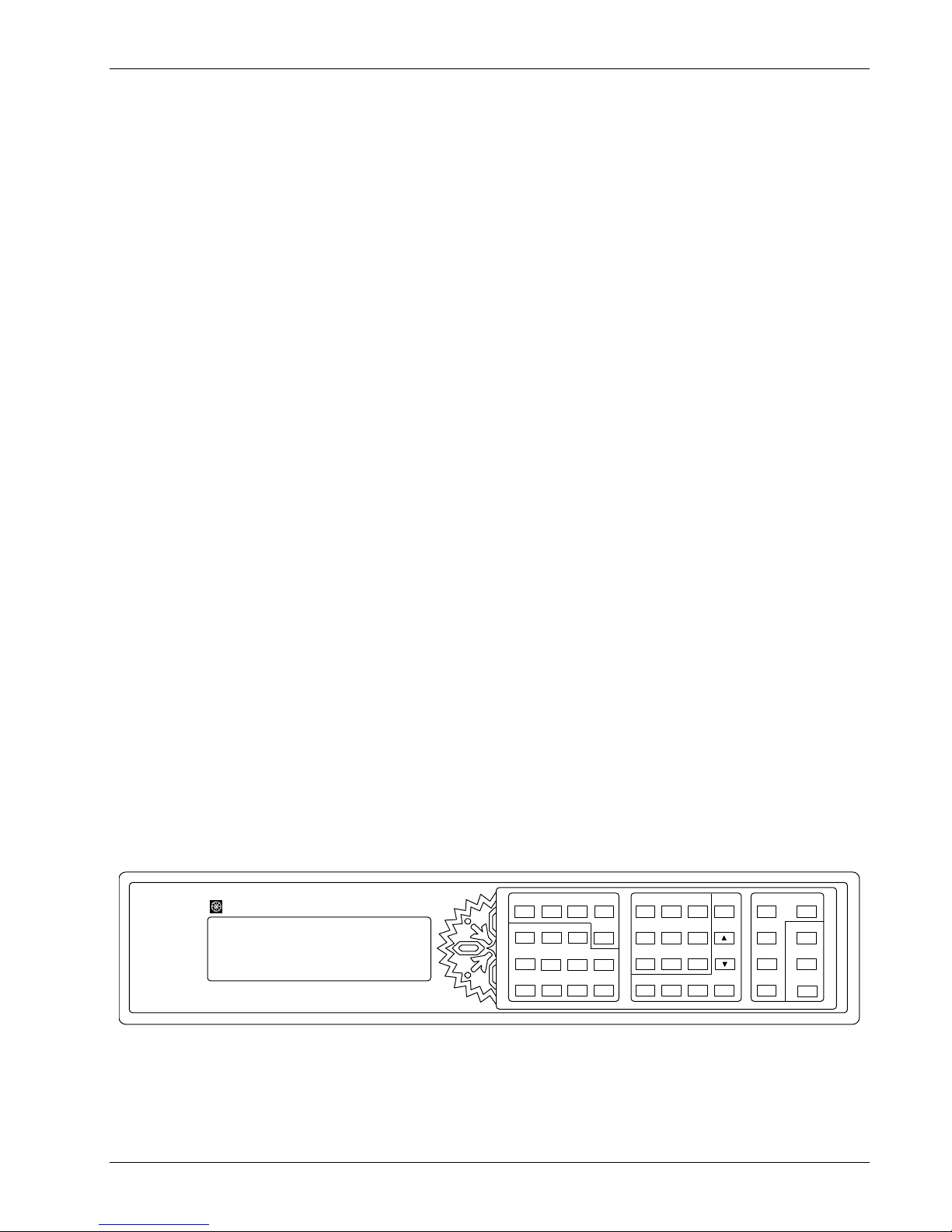
Figure 1-1. Model 340 Front Panel
Input
Setup
Scan
Setup
Alarm
Setup
Alarm
Reset
Display
SoftCal
Format
789
Curve
Inte r f a ce
Ent r y
456
Analog
Math
Outputs
Setup
123
Math
Options
Reset
0
+/-
.
+/-
Cance l
Escape
Sc r e en M o r e
Previous
Setting
Loca l
Next
DataCard
Setting
Save
Ent er
Help
Sc r e en
Page 14
Lake Shore Model 340 Temperature Controller User’s Manual
1.1 TEMPERATURE CONTROL SYSTEM
The goal of a temperature control system is to balance the effect of heating and cooling to provide a stable
temperature in an area of interest. In order to control temperature, you need the following elements:
1. A heating source.
2. A cooling source.
3. A means to measure temperature.
4. A means to compare the measured temperature to a desired temperature (called the setpoint).
5. A means to make any necessary changes to either the heating, the cooling, or both.
One familiar example is the temperature control system in a typical home. When the outside temperature
(cooling source) lowers the temperature inside (area of interest) below the temperature setting (desired
temperature) the thermostat measures the temperature and detects the difference (comparison) and turns on
the furnace (changes heat source). Substituting some control jargon would result in the description of a
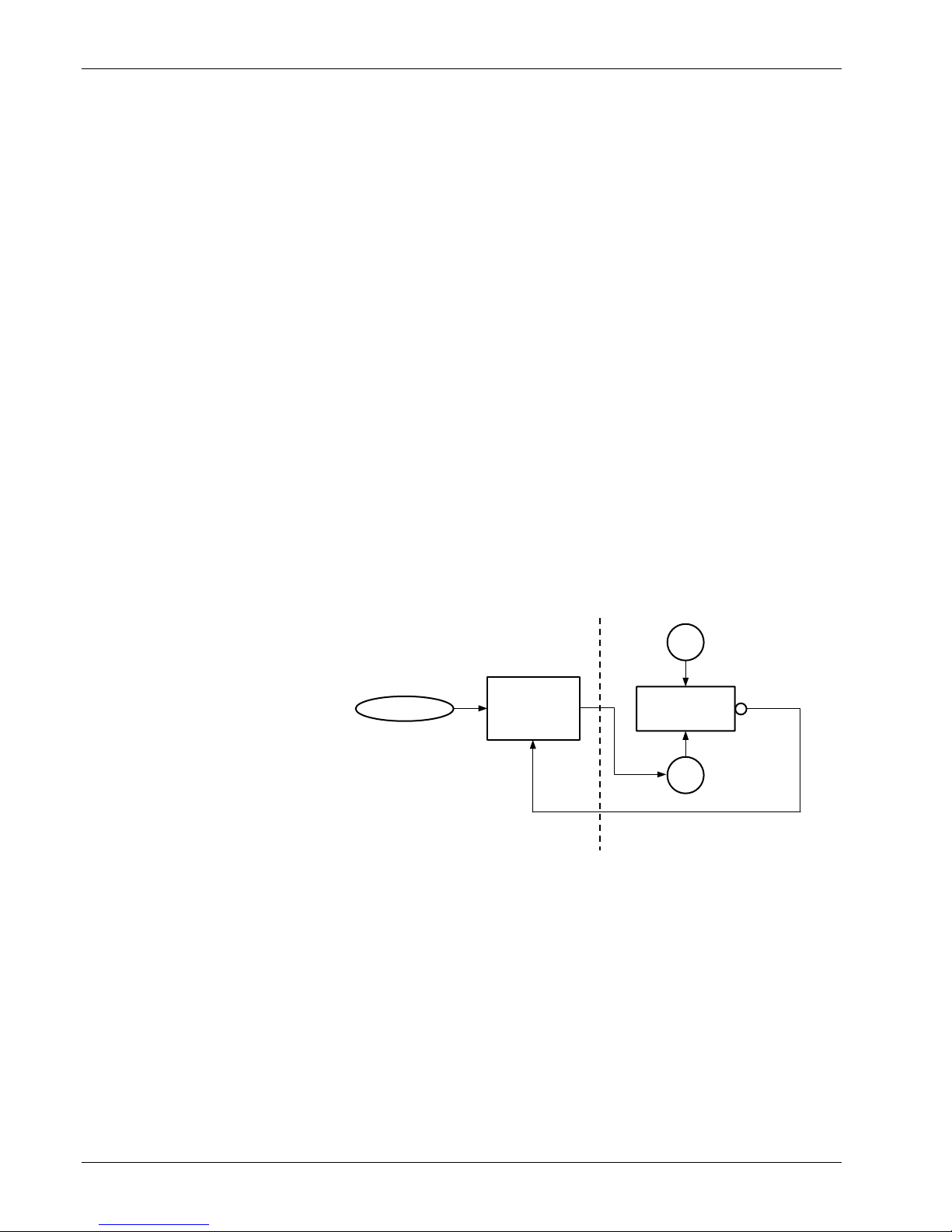
temperature control loop: When the cooling source reduces the temperature of the load below the
setpoint, a temperature sensor provides feedback to the control equation which detects the error and
actuates the heat source.
In our house example, there is only one actuator: the heat of the furnace. If the house is equipped with air
conditioning, the cooling source is a second actuator allowing control over a greater range of temperature. All
of the parts are called a closed loop control system and the operation is referred to as a control loop
because there is a cycle of cause and effect: From the control equation to the actuator to the load to the
sensor to the control loop and so on. The loop operation allows the heat source to turn on and off repeatedly,
keeping the temperature constant over a long period of time.
1.2 TEMPERATURE CONTROL SYSTEM WITH THE MODEL 340
The Model 340 is designed to work
as an integral part of a cryogenic
temperature control system (as
Cooling Source
(Cryogen)
described in Paragraph 1.1). The
Model 340 has many specialized
features that uniquely qualify it for
this difficult job. These features are
built on a fundamentally sound
design that can be used in many
applications requiring stable and
Setpoint
Temp erature
You Want
Model 340
(Control
Equation)
Load
(Cryostat)
Heater
Sensor
(Actual Temp.)
accurate control from cryogenic
temperatures, to room temperature
and above. Much of the information
in this manual refers to cryogenic
Warm Side Cold Side
Feedback
systems, but the ideas generally
apply at any temperature.
Figure 1-2. Typical Temperature Control System With Model 340
1.2.1 Cooling Source
The Model 340 integrates many of the elements of a complete control system. There are a few parts that the
Model 340 does not provide. The largest and most notable part missing is a cooling source. The Model 340
provides power to a resistive heater acting as the heating source, but it does not provide cooling. When
operating at cryogenic temperatures a vacuum insulated cryostat or dewar typically provides cooling power to
a relatively small load that may be a block of copper or other thermally conductive material. The load has a
sample holder or mounting surface for the material that is being studied. Sample holders are often custom
made for individual experiments.
1-2 Introduction
Page 15

Cooling Source (Continued)
Lake Shore Model 340 Temperature Controller User’s Manual
The load must also accommodate a temperature sensor for feedback and a resistive heater for heating. The
sensor and heater are in thermal contact with the cooled load while the Model 340 stays at room temperature.
There are a large number of combinations of loads, sensors, and heaters to meet different sample and
experimental requirements. For this reason, sensors and heaters are not included with the instrument but are
either included with the cooling system or sold separately. Lake Shore has the most comprehensive line of
temperature sensors in the industry, and the Model 340 will work with most of them. Heaters and other
accessories are also available.
1.2.2 Feedback
Temperature sensing is important to the feedback parts of a control system as well as an important
experimental parameter. The sensitivity of a sensor in the temperature range plays a critical role in the
accuracy and resolution of the measurement as well as the control stability. The Model 340 provides current
to (excites) the sensors and measures the resulting signal. The signal is converted to temperature by
comparing it to a temperature response curve that is stored in the instrument. Every effort is made within the
instrument to keep the measurement as accurate and quiet as possible. Temperature feedback begins the
role of the Model 340 in a control system.
1.2.3 Control Equation
The Model 340 can implement a control equation with an algorithm that calculates the amount of heating
needed to keep the load at the setpoint temperature. For most systems the cryostat or other cooling source is
running all of the time. It is necessary to tune the control equation because cooling sources and loads are
different. The Model 340 provides several different tuning options for choosing the best control settings. An
improperly tuned system will either not stabilize or will stabilize at a temperature below the setpoint.
1.2.4 Heating
Once the control equation computes the adjustment needed in heating, the Model 340 implements it by
changing the amount of current being sent to the resistive heater. There are significant differences between
the Model 340 and a home thermostat. First, the Model 340 can source the necessary power with an internal
direct current (DC) power supply while a thermostat depends on the furnace to provide heating power.
Second the Model 340 can make small adjustments in power to maintain a stable continuous temperature.
A thermostat can only turn the furnace on and off creating a abrupt change in temperature that includes
warming above the setpoint then cooling below. The heater output of a Model 340 can be optimized for
individual systems with heater ranges and limits.
1.3 MODEL 340 FEATURES
The following chapters of this manual are intended to help integrate the Model 340 into a temperature control
system with the fundamental building blocks described in Paragraph 1.2. This section is a brief overview of
some individual features of the instrument that may not be obvious in the setup and operation sections. These
features illustrate the Lake Shore goal of making the Model 340 a valuable part of the temperature control
environment. See Figure 1-3.
1.3.1 Configurable Inputs
Each of the many different types of temperature sensor has qualities that make it the best choice for some
application. The Model 340 has the ability to operate with many different types of sensors so that it is not a
limiting factor when deciding which sensor to use. The two sensor inputs included in the Model 340 can be
configured to measure and control with nearly any diode or resistive sensor. Appropriate excitation and input
gain can be selected from the front panel. There are no modules or cards to swap or internal switches to
change. Resistive sensors that change many orders of magnitude are measured in an autorange mode that
keeps the power in the sensor low to reduce self heating. The Model 340 does require the installation of an
option card to read sensors other than diodes and resistors or to read more than two inputs continuously.
Introduction 1-3
Page 16

Lake Shore Model 340 Temperature Controller User’s Manual
Power Supply
Heater
Digital
AC Line
Rear
Pane l
Sensor A
Rear
Pane l
Input
IEEE-488
Sensor B
Input
A
Input
B
A/D
A/D
Input
µP
Isolation
386EX
µP
Code
Serial
Analog Out 1
Analog Out 2
High Alarm Relay
Low Alarm Relay
Digital I/O
Memory Card
Flash
High Power
Heater
Current Source
D/A
Heater
A/D
Meter
Isolation
Isolation
Curve
Flash
SRAM
Keypad
Display
Front
Pane l
NOVRAM
340-1-3.eps
Figure 1-3. Model 340 Temperature Controller Block Diagram
1.3.2 Input Isolation
The sensor inputs on the Model 340 are isolated from chassis and earth ground to minimize the amount of
earth ground reference noise on the sensor input leads and in the sensor measurement. The two sensor
inputs included in the Model 340 make differential measurements and share their isolated input ground. If an
option is added to the Model 340 it may have its own isolated ground. The heater output is also isolated from
earth ground and from the sensor inputs to minimize interaction between the heater output and any other
circuitry. Figure 1-3 illustrates the isolation boundaries.
1.3.3 Input Reading Capability
The Model 340 is well suited to measure temperature in addition to controlling. Sensor inputs are read
constantly with a high-resolution analog-to-digital converter (A/D) that is dedicated to that input. Data from the
ADC is converted to temperature using a temperature response curve for the sensor. Temperature readings
and raw sensor readings are always available for every input and can be displayed, sent over computer
interface or used for one of the many built in features of the Model 340. New readings are taken as often as
20 times a second, the update rate is slower for more complex readings. The display is updated more slowly
than data is read because the flicker of fast changes is distracting. Readings are available at full speed over
computer interface.
1-4 Introduction
Page 17

Lake Shore Model 340 Temperature Controller User’s Manual
1.3.4 Temperature Response Curves and CalCurves™
A temperature response curve is needed to convert a sensor readings to temperature. Some types of sensors
share the same response and have a standard curve. The Model 340 includes standard curves for several
sensors. If an application requires more accuracy or a standard curve is not available, a specific curve must
be loaded into the instrument for an individually calibrated sensor. Lake Shore offers a broad range of
calibrated sensors and a CalCurve service that helps get calibration data into the instrument. The Model 340
provides several ways to load curves from Lake Shore calibrations or user supplied sensors. Any curve can
be entered from the front panel or over computer interface. CalCurves hold a copy of a curve called a
breakpoint interpolation table and are installed at the factory when purchased with a Model 340, or they can
be field installed using the data card slot.
1.3.5 SoftCal™
SoftCal is a good solution for applications that need more accuracy than a standard curve, but need no
traditional calibration. SoftCal is an algorithm that utilizes the predictability of standard curves to improve the
accuracy of an individual sensor around a few known temperature reference points. SoftCal generated curves
can be purchased with some types of sensors. The Model 340 also generates SoftCal curves.
1.3.6 Configurable Heater Output
The heater output is the most visible Model 340 control function because heater action is in direct opposition
with the cooling system. The Model 340 can source up to 100 watts of variable DC power to control Loop 1.
For good control, heater power should complement cooling power. For example a heater output may need a
range of 0 to 25 watts to work well with a cooling source that is 10 watts. Heating power is determined by the
resistance of the heater and the current being sent to it. Heater resistance is usually fixed once installed, so
the Model 340 heater output has several current ranges. These ranges allow different powers without the loss
of control resolution. The Model 340 allows for heaters of different resistance, but at highest power the choice
of resistance is limited.
1.3.7 Heater Output Protection
Cryostats have delicate sensors and wiring that can be damaged if over heated. Features have been added
to the Model 340 to minimize the possibility of over heating. These include setpoint temperature limit, heater
current range limit, internal heater diagnostics and a fuse in the heater output wiring.
1.3.8 Second Control Loop
When a instrument can run one closed loop control system it is referred to as a single loop controller. The
Model 340 has a the ability to run a second, independent control loop so it is called a two loop controller. The
second loop is used more often to reduce the temperature gradients in one cooling system than run two
different cooling systems. Even in well designed systems temperature gradients can be too large for some
experiments. The second loop can be used to control the temperature of radiation shields and other physical
structures or to control a small heater close to the sample while a large heater controls the load. The second
loop has much less power than the first loop and a few less software features.
1.3.9 AutoTune
Selecting the appropriate control settings (tuning) is a sometimes frustrating and tedious task. The AutoTune
feature can help by choosing a workable set of control settings on most systems. The AutoTune feature is
only available one control loop at a time.
1.3.10 Setpoint Ramping and Zones
In some applications getting to a controlled temperature is as important as being there. The setpoint ramp
feature allows smooth continuous changes in setpoint. With this feature data can be taken as the system is
changing in temperature for faster experiment cycles. It can also be used to make the approach to a setpoint
temperature more predictable. Ramping over large temperature changes may require different control settings
and the zone feature will change them automatically. Control settings for several different temperature zones
can be loaded in the Model 340 and the proper settings are used for any new setpoint.
Introduction 1-5
Page 18
Lake Shore Model 340 Temperature Controller User’s Manual
1.3.11 Internal Programming
The Model 340 can run a set of instrument instructions called an internal program. Each program represents
the temperature changes needed to do a users experiment. Setpoint can be changed or ramped up and down
and other controller parameters can be programmed. For simple experiments the internal program eliminates
the need for computer control. It is also common for the internal program to be used with computer control so
the computer is not slowed down by temperature control overhead.
1.3.12 Math
Some math features are included to improve usability and aid in setting up experiments. It can be useful to
have reading filters and maximum and minimum calculations easily available on the front panel. The Model
340 also computes a linear equation on reading data to allow some flexibility in how the display represents
experimental inputs. The Model 340 does not include the ability to do significant data manipulation. Serious
numerical analysis must be done off line.
1.3.13 Alarms, Analog Outputs, and Digital I/O
A clear example of the commitment to making the Model 340 a real part of the experimental environment is
the inclusion of analog and digital (TTL level) inputs and outputs. These features are not needed for a typical
temperature control loop but they provide an effective interface to other experimental hardware at relatively
low cost to the user. Relays can be tied to temperature alarms or opened and closed manually. Analog
outputs can transmit temperature to data recorders or be used as a variable voltage source. Digital inputs and
outputs can improve the efficiency of external sensor scanning or be used to set and monitor system function.
1.3.14 Memory Card
A memory card slot conforming to PCMCIA pin out is included for special instrument applications. The slot is
not a general purpose PCMCIA interface. Supported applications include data logging, curve transfer and
loading, saving and restoring instrument setup.
1.3.15 Computer Interface
The Model 340 has two types of computer interfaces. The parallel interface conforms to IEEE-488.2 standard
unless otherwise specified. The IEEE-488 interface is high speed and allows for multiple instruments to
communicate on the same bus. It is commonly used with laboratory instrumentation. Necessary interface
hardware is not included with most personal computers so it must be added with a third party card.
The serial interface conforms to
RS-232C electrical format included
with most personal computers. Serial
interfaces are much faster now than
they were just a few years ago but
this interface is less common in
laboratories because only one
instrument can communicate per
channel.
Either interface can send settings to
the Model 340 and collect reading
data back from it. Every attempt is
made to allow full access to
instrument features so it can be fully
involved in computer controlled
experiments. Even the analog
outputs and digital inputs and outputs
(I/O) can be controlled by computer
interface.
Control Output Heater Output Analog Output 2
Maximum Output Power 100 W 1 W
Output Type Current Source Voltage Source
Multiple Output Ranges Yes No
PID Control Yes Yes
AutoTune Yes Yes
Zone Tuning Yes Yes
Ramping Yes Yes
Internal Programming Yes No
Open Loop Control Yes Yes
Display in Current or Power Yes No
Large Display Yes Yes
Setpoint Limit Yes Yes
Slope Limits Yes Yes
Heater Range Limit Yes No
Table 1-1. Comparison of Control Loops 1 and 2
Hardware Features Loop 1 Loop 2
Software Features Loop 1 Loop 2
Control Loop Filter Yes Yes
1-6 Introduction
Page 19

Lake Shore Model 340 Temperature Controller User’s Manual
Thermometry:
Number of Inputs: Two included, more optional
Measurement Type: Four-lead Differential
Standard Sensor Inputs: Silicon Diode, GaAIAs Diode, Platinum RTD, Cernox RTD, Germanium RTD,
Carbon-Glass RTD, Ruthenium Oxide, Rhodium Iron, other resistive sensors
Optional Sensor Inputs: Thermocouple, Capacitance
Input Accuracy: Sensor Dependent. Refer to Table 1-2
A/D Resolution: 24-bit Analog-to-Digital
Update Rate: Up to 20 readings/second on an input, 40 readings/second on all inputs
Standard Curves 11 standard curves
User Curve Storage: Forty 200-point CalCurves or user curves
SoftCal: Improves accuracy of DT-470 diode or platinum RTD sensors.
Math: Maximum and Minimum of input readings and linear equation.
Filter: Averages input readings to quiet display, settable time constant,
can average from 2 to 64 input readings
Control:
Control Loops: Two
Control Type: Digital PID with Manual output
Control Stability: Sensor Dependent, refer to Table 1-2
Heater Output (Loop 1 Only):
Heater Output Type: Variable DC current source
Heater Output Resolution: 18-bit Digital-to-Analog converter
Max. Heater Power: 100 W (2 A into 25 Ω load)
Max. Heater Output Current: 2 A
Current Limit Settings: 2 A, 1 A, 0.5 A, 0.25 A
Heater Output Compliance: 50 V
Heater Output Ranges: Five in decade steps of power
Heater Load Type: Resistive
Heater Load Range: 10 Ω to 100 Ω, 25 Ω for max heater power
Heater Noise: 50 µV + 0.001% of output voltage
PID Control Settings:
Gain (Proportional): 0-1000 with 0.1 setting resolution
Reset (Integral): 1-1000 with 0.1 setting resolution
Rate (Derivative): 1-1000 seconds with 1 second resolution
Manual Output: 0-100% with 0.01% setting resolution
Zone Control Mode: 10 temperature zones with control parameters
Setpoint Ramping: 0.1
– 100 K/minute
Internal Program: 100 program steps
Front Panel:
Display Type Graphic LCD with fluorescent backlight
Number of Input Displays: One to eight
Display Units: Temperature in K, °C, or sensor units V, mV, Ω, kΩ, nF
Display Resolution Input Temp: 0.0001 K below 10 K, 0.001 K above 10 K
Display Resolution Sensor Units: Sensor dependent, to six digits
Setpoint Setting Resolution: Same as display resolution (actual resolution is sensor dependent)
Heater Output Display: Numeric display in percent of full scale for power or current. Bar graph display of Heater
Output available.
Keypad: Numeric plus special function
Curve Entry: Front panel curve entry
Interfaces:
IEEE-488.2 Interface: SH1, AH1, T5, L4, SR1, RL1, PP0, DC1, DT0, C0, E1
Serial Interface: RS-232C electrical format, 19,200 baud, RJ-11 connector
Analog outputs: Temperature monitor or Loop 2 control output
Number: Two
Voltage Range: ±10 volts
Resolution: 1.25 mV
Maximum Current: 0.1 amperes
Minimum Load: 100 Ω
Alarm Type: High and low alarm for each input
Alarm Actuators: Audible beeper or relays
Relays:
Number: Two
Contacts Available: Normally open (N.O.), normally closed (N.C.), and common (C)
Contact Rating: 30 VDC at 2 A
Digital I/O: 5 inputs and 5 outputs. TTL voltage level compatible
Data Card: PC card Type II slot used for curve transfer, setup storage, and data logging
General:
Ambient Temperature Range: 20
– 30 °C (68 – 86 °F) for specified accuracy; 15 – 35 °C (59 – 95 °F) for reduced accuracy
Power Requirements: 100, 120, 220, 240 VAC (+5%, –10%), 50 or 60 Hz; 190 VA
Enclosure Type: Full 19-inch Rack Mount
Size: 432 mm × 89 mm × 381 mm (17 × 3.5 × 15 inches)
Weight: 8 kilograms (17.6 pounds)
Introduction 1-7
Page 20
Lake Shore Model 340 Temperature Controller User’s Manual
Sensor Type Silicon Diode GaAlAs Diode
Table 1-2. Model 340 Sensor Input Performance Chart
100 Ω Platinum RTD
250 Ω Full scale
100 Ω Platinum RTD
500 Ω Full scale
1000 Ω
Platinum RTD
Temperature Coefficient Negative Negative Positive Positive Positive
Sensor Units Volts (V) Volts (V)
Input Range 0 - 2.5 V 0 – 7.5 V
Ohms (Ω) Ohms (Ω) Ohms (Ω)
0 – 250 Ω 0 – 500 Ω 0 – 2500 Ω
Sensor Excitation (Constant Current) 10 µA ±0.01% 10 µA ±0.01% 1 mA 1 mA 0.1 mA
Display Resolution Sensor Units 10 µV 10 µV
Example Lake Shore Sensor
DT-470-CO-13 with
1.4H calibration
TG-120SD with 1.4H
calibration
1 mΩ 1 mΩ 10 mΩ
PT-103 with 14J
calibration
PT-103 with 14J
calibration
PT-1001
calibration
*
with 1.4G
Temperature Range 1.4 – 475 K 1.4 - 475 K 30 – 675 K 30 – 800 K 30 – 675 K
Standard Sensor Curve Lake Shore
Curve 10
Typical Sensor Sensitivity
†
-30 mV/K at 4.2 K
-1.9 mV/K at 77 K
-2.4 mV/K at 300 K
-2.2 mV/K at 475 K
Measurement Resolution:
Sensor Units
Temperature Equivalence
10 µV
0.4 mK at 4.2 K
5.5 mK at 77 K
4.2 mK at 300 K
4.5 mK at 475 K
Electronic Accuracy:
Sensor Units
Temperature Equivalence
±80 µV ±0.005%
of reading
±5 mK at 4.2 K
±70 mK at 77 K
±50 mK at 300 K
±40 mK at 475 K
Temperature Accuracy including
electronic accuracy, CalCurve
and calibrated sensor
Control Stability:
Sensor Units
Temperature Equivalence
±27 mK at 4.2 K
±110 mK at 77 K
±85 mK at 300 K
±150 mK at 475 K
±20 µV
±0.8 mK at 4.2 K
±11 mK at 77 K
±8.4 mK at 300 K
±9 mK at 475 K
Magnetic Field Use
Recommended for
T ≥ 60 K and B ≤ 3 T
Requires calibrated
sensor
-180 mV/K at 10 K
-1.25 mV/K at 77 K
-2.75 mV/K at 300 K
-2.75 mV/K at 475 K
10 µV
0.1 mK at 10 K
8.0 mK at 77 K
3.6 mK at 300 K
3.6 mK at 475 K
±80 µV ±0.01%
of reading
±3 mK at 10 K
±150 mK at 77 K
±75 mK at 300 K
±55 mK at 475 K
±23 mK at 10 K
±195 mK at 77 K
±120 mK at 300 K
±165 mK at 475 K
±20 µV
±0.2 mK at 10 K
±16 mK at 77 K
±7.2 mK at 300 K
±7.2 mK at 475 K
Recommended for
T > 4.2 K & B ≤ 5 T
DIN 43760 DIN 43760 Scaled from
DIN 43760
0.19 Ω /K at 30 K
0.42 Ω /K at 77 K
0.39 Ω /K at 300 K
0.34 Ω /K at 675 K
1 mΩ
5.3 mK at 30 K
2.4 mK at 77 K
2.6 mK at 300 K
3.0 mK at 675 K
±0.002 Ω ±0.01%
of reading
±16 mK at 30 K
±10 mK at 77 K
±31 mK at 300 K
±82 mK at 675 K
±26 mK at 30 K
±20 mK at 77 K
±51 mK at 300 K
±182 mK at 675 K
±2 mΩ
±11 mK at 30 K
±4.8 mK at 77 K
±5.2 mK at 300 K
±6.0 mK at 675 K
Recommended for
T > 40 K & B ≤ 2.5 T
0.19 Ω /K at 30 K
0.42 Ω /K at 77 K
0.39 Ω /K at 300 K
0.33 Ω /K at 800 K
1 mΩ
5.3 mK at 30 K
2.4 mK at 77 K
2.6 mK at 300 K
3.0 mK at 800 K
±0.002 Ω ±0.01%
of reading
±16 mK at 30 K
±10 mK at 77 K
±31 mK at 300 K
±82 mK at 800 K
±26 mK at 30 K
±20 mK at 77 K
±51 mK at 300 K
±182 mK at 800 K
±2 mΩ
±11 mK at 30 K
±4.8 mK at 77 K
±5.2 mK at 300 K
±6.0 mK at 800 K
Recommended for
T > 40 K & B ≤ 2.5 T
1.9 Ω /K at 30 K
4.2 Ω /K at 77 K
3.9 Ω /K at 300 K
3.4 Ω /K at 675 K
10 mΩ
5.3 mK at 30 K
2.4 mK at 77 K
2.6 mK at 300 K
3.0 mK at 675 K
±0.03 Ω ±0.02%
of reading
±26 mK at 30 K
±17 mK at 77 K
±59 mK at 300 K
±161 mK at 675 K
±36 mK at 30 K
±27 mK at 77 K
±79 mK at 300 K
±261 mK at 675 K
±20 mΩ
±11 mK at 30 K
±4.8 mK at 77 K
±5.2 mK at 300 K
±6.0 mK at 675 K
Recommended for
T > 40 K & B ≤ 2.5 T
* No longer available from Lake Shore.
† Typical sensor sensitivities were taken from representative calibrations for the sensor listed.
1-8 Introduction
Page 21

Lake Shore Model 340 Temperature Controller User’s Manual
Table 1-2. Model 340 Sensor Input Performance Chart (Continued)
Sensor Type Rox™ Thermox™ Carbon-Glass™ Cernox™ Germanium
Temperature Coefficient Negative
Sensor Units
Ohms (Ω) Ohms (Ω) Ohms (Ω) Ohms (Ω) Ohms (Ω)
Input Range 10 ranges from
10 Ω to 300 kΩ
Sensor Excitation (Constant Current) 10 mV maximum
(10 current settings
from 30 nA to 1 mA)
Negative
10 ranges from
(1)
10 Ω to 300 kΩ
10 mV maximum
(10 current settings
from 30 nA to 1 mA).
Negative Negative Negative
10 ranges from
*
10 Ω to 300 kΩ*
10 mV maximum
(10 current settings
from 30 nA to 1 mA)
10 ranges from
10 Ω to 300 kΩ*
10 mV maximum
(10 current settings
from 30 nA to 1 mA)
10 ranges from
1 Ω to 30 kΩ
1 mV maximum
(10 current settings
from 30 nA to 1 mA)
Display Resolution Sensor Units Six digits Six digits Six digits Six digits Six digits
Example Lake Shore Sensor
RX-102A-AA with
0.3E calibration
TX-104-GB with 70L
calibration
CGR-1-500 with 1.4L
calibration
CX-1050-SD with 1.4L
calibration
GR-200A-100 with
0.3 A calibration
Temperature Range 0.3 – 200 K 70 – 325 K 1.4 – 325 K 0.3 – 325 K 0.3 – 40 K
Standard Sensor Curve Requires calibrated
sensor
Typical Sensor Sensitivity†
-16 kΩ/K at 0.3 K
-80 Ω/K at 4.2 K
-4 Ω/K at 20 K
-0.3 Ω/K at 77 K
Measurement Resolution:
Sensor Units
Temperature Equivalence
6 digits above 10 Ω
0.1 mK at 0.3 K
0.3 mK at 4.2 K
5 mK at 20 K
70 mK at 77 K
Electronic Accuracy:
Sensor Units
Temperature Equivalence
±0.02% RNG
±0.05% RDG
10 Ω to 80 kΩ.
±0.02% RNG
±0.2% RDG >80kΩ
±0.5 mK at 0.3 K
±16 mK at 4.2 K
±275 mK at 20 K
±3700 mK at 77 K
Temperature Accuracy including
electronic accuracy, CalCurve
and calibrated sensor
Control Stability:
Temperature Equivalence
±5.5 mK at 0.3 K
±28 mK at 4.2 K
±385 mK at 20 K
±4900 mK at 77 K
±0.2 mK at 0.3 K
±0.6 mK at 4.2 K
±10 mK at 20 K
±150 mK at 77 K
Magnetic Field Use
Recommended for
T > 2 K and B ≤ 10 T
Requires calibrated
sensor
-9.5 kΩ/K at 77 K
-780 Ω/K at 100 K
-0.78 Ω/K at 200 K
-0.035 Ω/K at 300 K
6 digits above 10 Ω
0.1 mK at 77 K
0.1 mK at 100 K
3 mK at 200 K
60 mK at 300 K
±0.02% RNG
±0.05% RDG
0 Ω to 80 kΩ.
±0.02% RNG
±0.2% RDG >80kΩ
±6.6 mK at 77 K
±8 mK at 100 K
±22 mK at 200 K
±100 mK at 300 K
±34.6 mK at 77 K
±29 mK at 100 K
±52 mK at 200 K
±160 mK at 300 K
±0.2 mK at 77 K
±0.2 mK at 100 K
±6 mK at 200 K
±120 mK at 300 K
Requires calibrated
sensor
-200 kΩ/K at 1.4 K
-706 Ω/K at 4.2 K
-0.15 Ω/K at 77 K
-0.015 Ω/K at 300 K
6 digits above 10 Ω
0.1 mK at 1.4 K
0.2 mK at 4.2 K
20 mK at 77 K
133 mK at 300 K
±0.02% RNG
±0.05% RDG
10 Ω to 80 kΩ.
±0.02% RNG
±0.2% RDG >80kΩ
±2 mK at 1.4 K
±2 mK at 4.2 K
±235 mK at 77 K
±2900 mK at 300 K
±7 mK at 1.4 K
±7 mK at 4.2 K
±285 mK at 77 K
±3150 mK at 300 K
±0.2 mK at 1.4 K
±0.4 mK at 4.2 K
±40 mK at 77 K
±300 mK at 300 K
Not recommended Recommended for
T > 2 K and B ≤ 19 T
Requires calibrated
sensor
-300 kΩ/K at 1.4 K
-10 kΩ/K at 4.2 K
-5 Ω/K at 77 K
-0.1 Ω/K at 300 K
6 digits above 10 Ω
0.1 mK at 1.4 K
0.1 mK at 4.2 K
0.5 mK at 77 K
20 mK at 300 K
±0.02% RNG
±0.05% RDG
10 Ω to 80 kΩ
±0.02% RNG
±0.2% RDG >80kΩ
±1 mK at 1.4 K
±2 mK at 4.2 K
±80 mK at 77 K
±400 mK at 300 K
±6 mK at 1.4 K
±7 mK at 4.2 K
±110 mK at 77 K
±450 mK at 300 K
±0.2 mK at 1.4 K
±0.2 mK at 4.2 K
±1 mK at 77 K
±40 mK at 300 K
Recommended for
T > 2 K and B ≤ 19 T
Requires calibrated
sensor
-209 kΩ /K at 0.3 K
-400 Ω /K at 1.4 K
-20 Ω /K at 4.2 K
-8.7 Ω /K at 6.0 K
6 digits above 1 Ω
0.1 mK at 0.3 K
0.1 mK at 1.4 K
0.3 mK at 4.2 K
0.6 mK at 6.0 K
±0.02% RNG
±0.1% RDG
10 Ω to 8 kΩ.
±1 mK at 0.3 K
±20 mK at 1.4 K
±25 mK at 4.2 K
±50 mK at 6.0 K
±6 mK at 0.3 K
±25 mK at 1.4 K
±30 mK at 4.2 K
±55 mK at 6.0 K
±0.2 mK at 0.3 K
±0.2 mK at 1.4 K
±0.6 mK at 4.2 K
±1.2 mK at 6.0 K
Not recommended
* Can be used below 3 Ω with reduced resolution and accuracy.
† Typical sensor sensitivities were taken from representative calibrations for the sensor listed.
Introduction 1-9
Page 22
Lake Shore Model 340 Temperature Controller User’s Manual
Sensor Type Thermocouple 25 mV Thermocouple 50
Table 1-2. Model 340 Sensor Performance Chart (Continued)
Capacitance 15 nF Capacitance 150 nF
mV
Temperature Coefficient Positive. Positive or Negative.
Sensor Units mV nF
Input Range ±25 mV ±50 mV 0-15 nF 0-150 nF
Sensor Excitation Not applicable. 4.88 kHz, 1V square wave
Display Resolution
Sensor Units
0.1 µV 0.1 pF 1 pF
Example Lake Shore Sensor AuFe0.07% vs. Cr CS-401LGB CS-501GR
Temperature Range 1.4 – 325 K.
1-60 K (pos)
80-300 K (neg)
1.4-290 K (pos)
Standard Sensor Curve By type. None.
Typical Sensor Sensitivity
*
16 µV/K at 4.2 K
20 µV/K at 300 K
66 pF/K at 4.2 K
7 pF/K at 60 K
31 pF/K at 4.2 K
58 pF/K at 77 K
197 pF/K at 200 K
Measurement Resolution:
Sensor Units
Temperature Equivalence
Electronic Accuracy†:
Sensor Units
Temperature Equivalence
0.2 µV
12 mK at 4.2 K
10 mK at 300 K
±1 µV ±0.05% RDG
80 mK at 4.2 K
50 mK at 300 K
0.4 µV
24 mK at 4.2 K
20 mK at 300 K
±1 µV ±0.05% RDG
100 mK at 4.2 K
60 mK at 300 K
0.2 pF
3 mK at 4.2 K
28 mK at 60 K
±50 pF ±0.1% RDG
0.84 K at 4.2 K
7.8 K at 60 K
2.0 pF
65 mK at 4.2 K
34 mK at 77 K
10 mK at 200 K
±50 pF ±0.1% RDG
1.8 K at 4.2 K
1 K at 77 K
0.36 K at 200 K
Temperature Accuracy
including electronic accuracy,
Calibration not available from Lake Shore.
Not applicable.
CalCurve, & calibrated sensor
Control Stability:
Sensor Units
Temperature Equivalence
0.4 µV
24 mK at 4.2 K
20 mK at 300 K
0.8 µV
50 mK at 4.2 K
40 mK at 300 K
±0.4 pF
6 mK at 4.2 K
56 mK at 60 K
±4 pF
130 mK at 4.2 K
68 mK at 77 K
20 mK at 200 K
Magnetic Field Use Thermocouple type dependent. Recommended for high field.
* Typical sensor sensitivities were taken from representative calibrations for the sensor listed.
† Accuracy specification does not include errors from room temperature compensation.
1-10 Introduction
Page 23

Lake Shore Model 340 Temperature Controller User’s Manual
CHAPTER 2
COOLING SYSTEM DESIGN
2.0 GENERAL
Selecting the proper cryostat or cooling source is probably the most important decision in designing a
temperature control system. The cooling source defines minimum temperature, cool-down time, and cooling
power. This chapter provides information on how to get the best temperature measurement and control from
cooling sources with proper setup including sensor and heater installation.
Chapter 2 contains the following major topics. Temperature sensor selection is covered in Paragraph 2.1.
Calibrated sensors are covered in Paragraph 2.2. Sensor installation is covered in Paragraph 2.3. Heater
selection and installation is covered in Paragraph 2.4. Considerations for good control are covered in
Paragraph 2.5. PID Control is covered in Paragraph 2.6. Manual Tuning is covered in Paragraph 2.7.
AutoTuning is covered in Paragraph 2.8. Finally, Zone Tuning is covered in Paragraph 2.9.
2.1 TEMPERATURE SENSOR SELECTION
This section is intended to help the user ask the proper questions about sensor selection, and not to give all
the answers. Additional useful information on temperature sensor selection is available in the Lake Shore
Temperature Measurement and Control Catalog. The catalog has a large reference section that includes
sensor characteristics and sensor selection criteria.
Temperature range is discussed in Paragraph 2.1.1. Sensor sensitivity is discussed in Paragraph 2.1.2.
Environmental conditions are discussed in Paragraph 2.1.3. Measurement accuracy is discussed in
Paragraph 2.1.4. Finally, sensor packages are discussed in Paragraph 2.1.5.
2.1.1 Temperature Range
Several important sensor parameters must be considered when choosing a sensor. The first is temperature
range. The experimental temperature range must be known when choosing a sensor. Some sensors can be
damaged by temperatures that are either too high or too low. Manufacturer recommendations should always
be followed.
Sensor sensitivity is also dependent on temperature and can limit the useful range of a sensor. It is important
not to specify a range larger than necessary. If an experiment is being done at liquid helium temperature and
a very high sensitivity is needed for good measurement resolution, that same resolution may not be required
to monitor warm up to room temperature. Two different sensors may be required to tightly cover the range
from helium to room temperature, but lowering the requirement on warm up may allow a less expensive, one
sensor solution.
Another thing to consider when choosing a temperature sensor is that instruments like the Model 340 are not
able to read some sensors over their entire temperature range. Lake Shore sells calibrated sensors that
operate down to 50 millikelvin (mK), but the Model 340 is limited to 300 mK in its standard configuration.
2.1.2 Sensor Sensitivity
Temperature sensor sensitivity is a measure of how much a sensor signal changes when the temperature
changes. It is an important sensor characteristic because so many measurement parameters are related to it.
Resolution, accuracy, noise floor, and even control stability depend on sensitivity. Many sensors have
different sensitivities at different temperatures. For example, a platinum sensor has good sensitivity at higher
temperatures but has limited use below 30 kelvin (K) because its sensitivity drops sharply. It is difficult to
determine if a sensor has adequate sensitivity over the experimental temperature range. This manual has
specifications (Table 1-1) that include sensor sensitivity translated into temperature resolution and accuracy
at different points. This is typical sensor response and can be used as a guide when choosing a sensor to be
used with the Model 340.
Cooling System Design 2-1
Page 24

Lake Shore Model 340 Temperature Controller User’s Manual
2.1.3 Environmental Conditions
Environmental factors such as high vacuum, magnetic field, corrosive chemicals, or even radiation may limit
the effectiveness of some sensors. Lake Shore has devoted much time to develop sensor packages that
withstand the environmental factors found in typical cryogenic cooling systems.
Magnetic field experiments are very common. Field dependence is an important selection criteria for
temperature sensors used in these experiments. Table 1-1 states the field dependence of most common
sensors. The Lake Shore Temperature Measurement and Control Catalog includes detailed field dependence
tables along with specific data on other environmental factors when available.
2.1.4 Measurement Accuracy
Temperature measurements have several sources of error that reduce accuracy. Be sure to account for
errors induced by both the sensor and the instrumentation when computing accuracy. The instrument has
measurement error in reading the sensor signal and error in calculating a temperature using a temperature
response curve. Error results from the sensor being compared to a calibration standard and the temperature
response of a sensor will shift with time and with repeated thermal cycling (from very cold temperatures to
room temperature). Instrument and sensor makers specify these errors but there are things a user can do to
maintain good accuracy. For example, choose a sensor that has good sensitivity in the most critical
temperature range, as sensitivity can minimize the effect of most error sources. Install the sensor properly
following guidelines in Paragraph 2.3. Have the sensor and instrument periodically recalibrated, or in some
other way null the time dependent errors. Use a sensor calibration appropriate for the accuracy requirement.
2.1.5 Sensor Package
There are many types of sensor packages which generally determine sensor size, thermal and electrical
contact to the outside, and sometimes limit temperature range. Some sensors may be purchased as bare
chips without a package. When different packages are available for a sensor, consider the sensor mounting
surface and how leads will be heat sinked.
2.2 CALIBRATED SENSORS
It can be difficult to choose the right sensor, calibrate it, translate calibration data into a temperature response
curve understandable to the Model 340, and load the curve into the instrument. Lake Shore offers a variety of
calibration and curve loading services to fit different accuracy requirements and budgets: traditional
calibration in Paragraph 2.2.1, SoftCal™ in Paragraph 2.2.2, standard curves in Paragraph 2.2.3, and the
Lake Shore CalCurve Service in Paragraph 2.2.4.
2.2.1 Traditional Calibration
Calibration compares a sensor with an unknown temperature response to an accepted standard. Lake Shore
temperature standards are traceable to the U.S. National Institute of Standards and Testing (NIST) or the
National Physical Laboratory in Great Britain. These standards allow Lake Shore to calibrate sensors from 50
mK to above room temperature. Calibrated sensors are more expensive than uncalibrated sensors.
Calibrated temperature sensors are the most accurate available from Lake Shore. Errors from sensor
calibration are almost always smaller than error contributed by the Model 340. The Lake Shore Temperature
Measurement and Control Catalog has complete accuracy specifications for calibrated sensors.
Calibrated sensors include measured test data printed and plotted, coefficients of a Chebychev polynomial
fitted to the data, and two tables of data points used as interpolation tables optimized for accurate
temperature conversion. The smaller table, called a breakpoint interpolation table, fits into instruments like the
Model 340 where it is called a temperature response curve. Install a curve into a Model 340 through a
CalCurve™ (Paragraph 2.2.4) or manually through the instrument front panel.
Note instrument specifications before ordering calibrated sensors. A calibrated sensor is required when a
sensor does not follow a standard curve if the user wishes to display in temperature. Otherwise the Model 340
operates in sensor units like ohms or volts. The Model 340 may not work over the full temperature range of
some sensors. The standard inputs are limited to operation above 300 mK even with sensors that can be
calibrated to 50 mK.
2-2 Cooling System Design
Page 25
Lake Shore Model 340 Temperature Controller User’s Manual
2.2.2 SoftCal™
SoftCal is a good solution for applications that do not require the accuracy of a traditional calibration. The
SoftCal algorithm uses the well behaved nature of sensors that follow a standard curve to improve the
accuracy of individual sensors. A few known temperature points are required to perform SoftCal.
Lake Shore sells SoftCal calibrated sensors that include both the large interpolation table and the smaller
breakpoint interpolation table. A CalCurve, described in Paragraph 2.2.4, may be required to get the
breakpoint table into a Model 340 where it is called a temperature response curve.
The Model 340 can also perform a SoftCal calibration. The user must provide one, two, or three known
temperature reference points. The range and accuracy of the calibration is based on these points.
Lake Shore DT-400 Series
There are 3 ways to improve
temperature sensor accuracy:
Silicon Diode Temperature Sensor
Standard
Standard sensors are interchangeable within the published tolerance band. Below are
Standard Curve 10 Tolerance
(Accuracy) Bands for DT-470.
Band
2 K* 100 K
11 ±0.25 K ±0.5 K ±1.0 K
11A ±0.25 K ±1% of Temp.
12 ±0.5 K ±1.0 K ±2.0 K
12A ±0.5 K ±1% of Temp.
13 ±1 K ±1% of Temp.
* Temps down to 1.4 K only with
Precision Calibrated Sensors.
To increase accuracy,
perform a SoftCal™ with the
controller and sensor. After
sensor calibration, the
custom curve for that sensor
replaces the standard Curve
10.
Generate a CalCurve™ for either
SoftCal™ or Precision Calibration.
100 K -
305 K
305 K -
375 K
SoftCal™ Calibration
A 2-point SoftCal™ uses data
points at 77.35 K and 305 K. A 3point SoftCal™ uses data points at
4.2 K, 77.35 K, and 305 K.
Typical 2-Point Accuracy
±1.0 K 2 K to <30 K
±0.25 K 30 K to <60 K
±0.15 K 60 K to <345 K
±0.25 K 345 K to <375 K
±1.0 K 375 K to 475 K
Typical 3-Point Accuracy
±0.5 K 2 K to <30 K
±0.25 K 30 K to <60 K
±0.15 K 60 K to <345 K
±0.25 K 345 K to <375 K
±1.0 K 375 K to 475 K
Enter the voltage at 2 or 3 data
points into a SoftCal™ capable
controller. A calibration report is
sent with the sensor.
CalCurve™
- or -
Precision Calibration
Lake Shore can calibrate most
sensors with up to 200 data points
and can concentrate data-taking in
specific areas of interest.
Typical Precision Cal. Accuracy
Temp. Typical Maximum
<10 K 12 mK 20 mK
10 K 12 mK 20 mK
20 K 15 mK 25 mK
30 K 25 mK 45 mK
50 K 30 mK 55 mK
100 K 25 mK 50 mK
300 K 25 mK 50 mK
340 K — 100 mK
480 K — 100 mK
Lake Shore fits a curve to these
points, and sends a detailed report
to the sensor that includes Raw
Temperature Data, Polynomial
Fits, and Interpolation Tables.
User calculates break-
points and manually enters
data into the controller
Model Number
8001
Breakpoint pairs
are factoryloaded in nonvolatile mem ory.
340-2-1.eps
Figure 2-1. Silicon Diode Sensor Calibrations and CalCurve
Cooling System Design 2-3
8000
Breakpoint pairs are
loaded on a Floppy Disk
in ACSII format for
Customer downloading.
3405-128F-CALCRV
Breakpoint pairs
are loaded in a
Datacard for field
installation.
Page 26

Lake Shore Model 340 Temperature Controller User’s Manual
2.2.3 Standard Curves
Some types of sensors behave in a very predictable manner and a standard temperature response curve can
be created for them. Standard curves are a convenient and inexpensive way to get reasonable temperature
accuracy. Sensors that have a standard curve are often used when interchangeability is important. Some
individual sensors are selected for their ability to match a published standard curve and sold at a premium,
but in general these sensors do not provide the accuracy of a calibrated sensor. For convenience, the Model
340 has several standard curves included in firmware.
2.2.4 CalCurve™
The CalCurve service provides the user with a convenient way get the temperature response curve from Lake
Shore calibrated sensors into instruments like the Model 340. It can be performed at the factory when
calibrated sensors and instruments are ordered together. The factory installed CalCurve option is Model 8001
and should be ordered with the calibrated sensor. A CalCurve can be done in the field when additional or
replacement sensors are installed. Curve data is loaded into some type of non-volatile memory that is
installed into the instrument by the user. In the case of the Model 340, the curve is loaded into a non-volatile
memory card which can be used for transfer into the instrument. The field installed version is a Model 3405128F-CALCRV and it should be ordered with the calibrated sensor. Customers that have a PC compatible
computer with an RS-232C or IEEE-488 interface have another option. The Model 8000 can also be ordered
with the calibrated sensor.
2.3 SENSOR INSTALLATION
This section highlights some of the important elements of proper sensor installation. For more detailed
information, Lake Shore sensors are shipped with installation instructions that cover that specific sensor type
and package. The Lake Shore Temperature Measurement and Control Catalog includes an installation
section as well. To further help users properly install sensors, Lake Shore offers a line of Cryogenic
Accessories. Many of the materials discussed are available through Lake Shore and can be ordered with
sensors or instruments.
Mounting materials is discussed in Paragraph 2.3.1. Sensor location is discussed in Paragraph 2.3.2. Thermal
conductivity is discussed in Paragraph 2.3.3. Contact area is discussed in Paragraph 2.3.4. Contact pressure
is discussed in Paragraph 2.3.5. Lead wire is discussed in Paragraph 2.3.6. Lead soldering is discussed in
Paragraph 2.3.7. Heat sinking leads is discussed in Paragraph 2.3.8. Finally, thermal radiation is discussed in
Paragraph 2.3.9.
2.3.1 Mounting Materials
Choosing appropriate mounting materials is very important in a cryogenic environment. The high vacuum
used to insulate cryostats is one source of problems. Materials used in these applications should have a low
vapor pressure so they do not evaporate or out-gas and spoil the vacuum insulation. Metals and ceramics do
not have this problem but greases and varnishes must be checked. Another source of problems is the wide
extremes in temperature most sensors are exposed to. The linear expansion coefficient of a materials
becomes important when temperature changes are so large. Never try to permanently bond materials with
linear expansion coefficients that differ by more than three. A flexible mounting scheme should be used or the
parts will break apart, potentially damaging them. The thermal expansion or contraction of rigid clamps or
holders could crush fragile samples or sensors that do not have the same coefficient. Thermal conductivity is
a property of materials that can change with temperature. Do not assume that a heat sink grease that works
well at room temperature and above will do the same job at low temperatures.
2.3.2 Sensor Location
Finding a good place to mount a sensor in an already crowded cryostat is never easy. There are less
problems if the entire load and sample holder are at the same temperature. Unfortunately, this not the case in
many systems. Temperature gradients (differences in temperature) exist because there is seldom perfect
balance between the cooling source and heat sources. Even in a well-controlled system, unwanted heat
sources like thermal radiation and heat conducting through mounting structures can cause gradients. For best
accuracy, sensors should be positioned near the sample, so that little or no heat flows between the sample
and sensor. This may not, however, be the best location for temperature control as discussed below.
2-4 Cooling System Design
Page 27
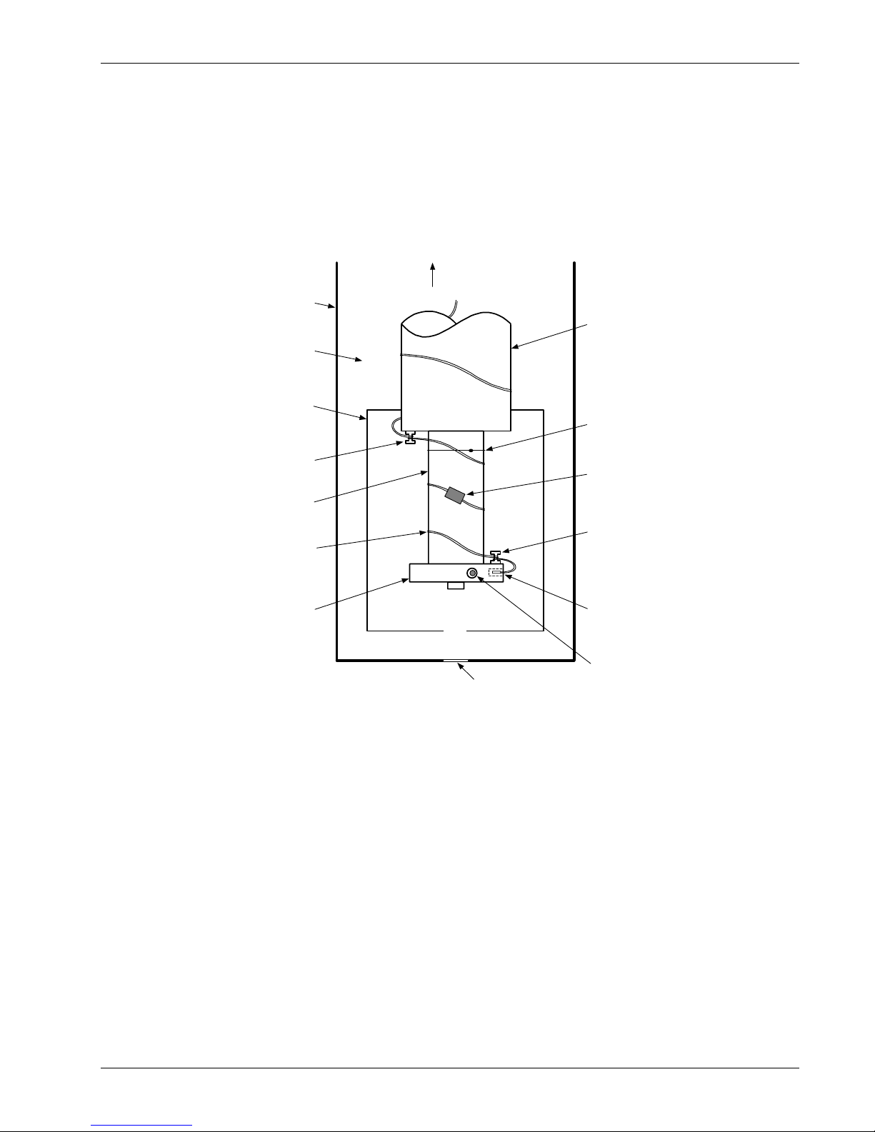
Lake Shore Model 340 Temperature Controller User’s Manual
2.3.3 Thermal Conductivity
The ability of heat to flow through a material is called thermal conductivity. Good thermal conductivity is
important in any part of a cryogenic system that is intended to be the same temperature. Copper and
aluminum are examples of metals that have good thermal conductivity, while stainless steel does not.
Non-metallic, electrically-insulating materials like alumina oxide and similar ceramics have good thermal
conductivity, while G-10 epoxy-impregnated fiberglass does not. Sensor packages, cooling loads, and sample
holders should have good thermal conductivity to reduce temperature gradients. Surprisingly, the connections
between thermally conductive mounting surfaces often have very poor thermal conductivity.
To Room
Temperature
Vacuum Shroud
Refrigerator
Vacuum Space
Radiation Shield
Thermal Anchor
(Bobbin)
Expander
Dental Floss
Tie-Down
-or-
Cryogenic Tape
Refrigerator
Stage
Second
Thermal Anchor
Cryogenic Wire
diameter,
(small
large AWG)
Cold Stage and
Sample Holder
Drawing
Not To Scale
340-2-2.eps
Optical Window
(If Required)
(Bobbin)
Sensor
Heater
(wirin g not sho wn
for clarity)
Figure 2-2. Typical Sensor Installation In A Mechanical Refrigerator
2.3.4 Contact Area
Thermal contact area greatly affects thermal conduction because a larger area has more opportunity to
transfer heat. Even when the size of a sensor package is fixed, thermal contact area can be improved with the
use of a gasket material. A soft gasket material forms into the rough mating surface to increase the area of
the two surfaces that are in contact. Good gasket materials are soft, thin, and have good thermal conductivity.
They must also withstand the environmental extremes. Indium foil and cryogenic grease are good examples.
2.3.5 Contact Pressure
When sensors are permanently mounted, the solder or epoxy used to hold the sensor act as both gasket and
adhesive. Permanent mounting is not a good solution for everyone because it limits flexibility and can
potentially damage sensors. Much care should be taken not to over heat or mechanically stress sensor
packages. Less permanent mountings require some pressure to hold the sensor to its mounting surface.
Pressure greatly improves the action of gasket material to increase thermal conductivity and reduce thermal
gradients. A spring clamp is recommended so that different rates of thermal expansion do not increase or
decrease pressure with temperature change.
Cooling System Design 2-5
Page 28

Lake Shore Model 340 Temperature Controller User’s Manual
2.3.6 Lead Wire
Different types of sensors come with different types and lengths of electrical leads. In general a significant
length of lead wire must be added to the sensor for proper heat sinking and connecting to a bulk head
connector at the vacuum boundary. The lead wire must be a good electrical conductor, but a poor thermal
conductor, or heat will transfer down the leads and change the temperature reading of the sensor. Small 30 to
40 AWG wire made of an alloy like phosphor bronze is much better than copper wire. Thin wire insulation is
preferred and twisted wire should be used to reduce the effect of RF noise if it is present. The wire used on
the room temperature side of the vacuum boundary is not critical so copper cable is normally used.
2.3.7 Lead Soldering
When additional wire is soldered to short sensor leads, care must be taken not to overheat the sensor. A heat
sink such as a metal wire clamp or alligator clip will heat sink the leads and protect the sensor. Leads should
be tinned before bonding to reduce the time that heat is applied to the sensor lead. Solder flux should be
cleaned after soldering to prevent corrosion.
2.3.8 Heat Sinking Leads
Sensor leads can be a significant source of error if they are not properly heat sinked. Heat will transfer down
even small leads and alter the sensor reading. The goal of heat sinking is to cool the leads to a temperature
as close to the sensor as possible. This can be accomplished by putting a significant length of lead wire in
thermal contact with every cooled surface between room temperature and the sensor. Lead wires can be
adhered to cold surfaces with varnish over a thin electrical insulator like cigarette paper. They can also be
wound onto a bobbin that is firmly attached to the cold surface. Some sensor packages include a heat sink
bobbin and wrapped lead wires to simplify heat sinking.
2.3.9 Thermal Radiation
Thermal (black body) radiation is one of the ways heat is transferred. Warm surfaces radiate heat to cold
surfaces even through a vacuum. The difference in temperature between the surfaces is one thing that
determines how much heat is transferred. Thermal radiation causes thermal gradients and reduces
measurement accuracy. Many cooling systems include a radiation shield. The purpose of the shield is to
surround the load, sample, and sensor with a surface that is at or near their temperature to minimize
radiation. The shield is exposed to the room temperature surface of the vacuum shroud on its outer surface,
so some cooling power must be directed to the shield to keep it near the load temperature. If the cooling
system does not include an integrated radiation shield (or one cannot be easily made), one alternative is to
wrap several layers of super-insulation (aluminized Mylar) loosely between the vacuum shroud and load. This
reduces radiation transfer to the sample space.
2.4 HEATER SELECTION AND INSTALLATION
There is a variety of resistive heaters that can be used as the controlled heating source for temperature
control. The mostly metal alloys like nichrome are usually wire or foil. Shapes and sizes vary to permit
installation into different systems.
Heater Resistance and power are discussed in Paragraph 2.4.1. Heater location is discussed in Paragraph
2.4.2. Heater types are discussed in Paragraph 2.4.3. Finally, heater wiring is discussed in Paragraph 2.4.4.
2.4.1 Heater Resistance and Power
Cryogenic cooling systems have a wide range of cooling power. The resistive heater must be able to provide
sufficient heating power to warm the system. The Model 340 can supply up to 100 W of power to a heater
(if the heater resistance is appropriate). The Model 340 heater output current source has a maximum output
of 2 A, limiting maximum power to: Max Power (watts) = (2 A)
2
× Resistance (ohms).
Even though the Model 340 output is a current source, it has a voltage limit (called the compliance voltage)
of 50 V, which also limits maximum power:
Max Power (watts)
= .
Resistance (ohms)
2-6 Cooling System Design
(50 volts)
2
Page 29

Heater Resistance and Power (Continued)
Lake Shore Model 340 Temperature Controller User’s Manual
Both limits are in place at the same time, so the smallest of the two computations gives the maximum power
available to the heater. A heater of 25 Ω allows the instrument to provide its maximum power of 100 watts.
A typical smaller resistance of 10 Ω allows 40 watts of power, while a typical larger resistance of 50 Ω allows
50 watts. The resistor chosen as a heater must be able to withstand the power being dissipated in it.
Pre-packaged resistors have a power specification that is usually given for the resistor in free air. This power
may need to be derated if used in a vacuum where convection cooling can not take place and it is not
adequately heat sinked to a cooled surface.
2.4.2 Heater Location
For best temperature measurement accuracy the heater should be located so that heat flow between the
cooling power and heater is minimized. For best control the heater should be in close thermal contact with the
cooling power. Geometry of the load can make one or both of these difficult to achieve. That is why there are
several heater shapes and sizes.
2.4.3 Heater Types
Resistive wire like nichrome is the most flexible type of heater available. The wire can be purchased with
electrical insulation and has a predictable resistance per given length. This type of heater wire can be
wrapped around a cooling load to give balanced, even heating of the area. Similar to sensor lead wire, the
entire length of the heater wire should be in good thermal contact with the load to allow for thermal transfer.
Heat sinking also protects the wire from over heating and burning out.
Resistive heater wire is also wound into cartridge heaters. Cartridge heater are more convenient but are bulky
and more difficult to place on small loads. A typical cartridge is ¼ inch in diameter and 1 inch long. The
cartridge should be snugly held in a hole in the load or clamped to a flat surface. Heat sinking for good
thermal contact is again important.
Foil heaters are thin layers of resistive material adhered to, or screened on to, electrically insulating sheets.
There are a variety of shapes and sizes. The proper size heater can evenly heat a flat surface or around a
round load. The entire active area should be in good thermal contact with the load, not only for maximum
heating effect, but to keep spots in the heater from over heating and burning out.
2.4.4 Heater Wiring
Small 30 AWG copper wire is recommended for heater leads inside of a vacuum shroud. Larger wire causes
too much heat to leak. These leads should be heat sunk similar to sensor leads so that heat leak does not
warm the load when the heater is not running. The lead wires should be twisted to minimize noise coupling
between the heater and other leads in the system. Outside the vacuum shroud larger copper cable should be
used but twisting is still recommended.
2.5 CONSIDERATIONS FOR GOOD CONTROL
Most of the techniques discussed above to improve cryogenic temperature accuracy apply to control as well.
There is an obvious exception in sensor location. A compromise is suggested below in the Two Sensor
Approach.
Thermal conductivity is discussed in Paragraph 2.5.1. Thermal lag is discussed in Paragraph 2.5.2. The twosensor approach is discussed in Paragraph 2.5.3. Thermal mass is discussed in Paragraph 2.5.4. Finally,
system nonlinearity is discussed in Paragraph 2.5.5.
2.5.1 Thermal Conductivity
Good thermal conductivity is important in any part of a cryogenic system that is intended to be at the same
temperature. Most systems begin with materials that have good conductivity themselves, but as sensors,
heaters, sample holders, etc., are added to an ever more crowded space, the junctions between parts are
often overlooked. In order for control to work well, junctions between the elements of the control loop must be
in close thermal contact and have good thermal conductivity. Gasket materials should always be used along
with reasonable pressure.
Cooling System Design 2-7
Page 30

Lake Shore Model 340 Temperature Controller User’s Manual
2.5.2 Thermal Lag
Poor thermal conductivity causes thermal gradients that reduce accuracy but they also cause thermal lag that
make it difficult for controllers to do their job. Thermal lag is the time it takes for a change in heating or cooling
power to propagate through the load and get to the feedback sensor. Because the feedback sensor is the
only thing that lets the controller know what is happening in the system, slow information to the sensor slows
the controllers response time. For example, if the temperature at the load drops slightly below the setpoint,
the controller gradually increases heating power. If the feedback information is slow, the controller puts too
much heat into the system before it is told to reduce heat. The excess heat causes a temperature overshoot,
degrading control stability. The best way to improve thermal lag is to pay close attention to thermal
conductivity both in the parts used and their junctions.
2.5.3 Two-Sensor Approach
There is a conflict between the best sensor location for measurement accuracy and the best sensor location
for control. For measurement accuracy the sensor should be very near the sample being measured which is
away from the heating and cooling sources to reduce heat flow across the sample and thermal gradients. The
best control stability is achieved when the feedback sensor is near both the heater and cooling source to
reduce thermal lag. If both control stability and measurement accuracy are critical it may be necessary to use
two sensors, one for each function. Many temperature controllers including the Model 340 have two sensor
inputs for this reason.
2.5.4 Thermal Mass
Cryogenic designers understandably want to keep the thermal mass of the load as small as possible so the
system can cool quickly and improve cycle time. Small mass can also have the advantage of reduced thermal
gradients. Controlling a very small mass is difficult because there is no buffer to adsorb small changes in the
system. Without buffering, small disturbances can very quickly create large temperature changes. There are
systems where it is necessary to add a small amount of thermal mass such as a copper block in order to
improve control stability.
2.5.5 System Nonlinearity
Because of nonlinearities in the control system, a system controlling well at one temperature may not control
well at another temperature. While nonlinearities exist in all temperature control systems, they are most
evident at cryogenic temperatures. When the operating temperature changes the behavior of the control loop,
the controller must be retuned. As an example, a thermal mass acts differently at different temperatures. The
specific heat of the load material is a major factor in thermal mass and the specific heat of materials like
copper change as much as three orders of magnitude when cooled from 100 K to 10 K. Changes in cooling
power and sensor sensitivity are also sources of nonlinearity.
The cooling power of most cooling sources also changes with load temperature. This is very important when
operating at temperatures near the highest or lowest temperature that a system can reach. Nonlinearities
within a few degrees of these high and low temperatures make it very difficult to configure them for stable
control. If difficulty is encountered, it is recommended to gain experience with the system at temperatures
several degrees away from the limit and gradually approach it in small steps.
Keep an eye on temperature sensitivity. Sensitivity not only affects control stability but it also contributes to
the overall control system gain. The large changes in sensitivity that make some sensors so useful may make
it necessary to retune the control loop more often.
2-8 Cooling System Design
Page 31

2.6 PID CONTROL
The Model 340 Temperature Controller uses a algorithm called PID control for closed-loop control operation.
The control equation for the PID algorithm has three variable terms, a P or proportional term, an I or integral
term, and a D or derivative term. See Figure 2-3. Changing these variables for best control of a system is
called tuning. The PID equation in the Model 340 is:
Lake Shore Model 340 Temperature Controller User’s Manual
Heater Output =+ +
Proportional (P) is discussed in Paragraph 2.6.1. Integral (I) is discussed in Paragraph 2.6.2. Derivative (D) is
discussed in Paragraph 2.6.3. Finally, the manual heater output is discussed in Paragraph 2.6.4.
2.6.1 Proportional (P)
The Proportional term, also called gain, must have a value greater than zero for the control loop to operate.
The value of the proportional term is multiplied by the error (e) which is defined as the difference between the
setpoint and feedback temperatures, to generate the proportional contribution to the output: Output (P) = Pe.
If proportional is acting alone, with no integral, there must always be an error or the output will go to zero. A
great deal must be known about the load, sensor, and controller to compute a proportional setting (P). Most
often, the proportional setting is determined by trial and error. The proportional setting is part of the overall
control loop gain, and so are the heater range and cooling power. The proportional setting will need to change
if either of these change.
2.6.2 Integral (I)
In the control loop, the integral term, also called reset, looks at error over time to build the integral contribution
to the output:
By adding the integral to proportional contributions, the error that is necessary in a proportional only system
can be eliminated. When the error is at zero, controlling at the setpoint, the output is held constant by the
integral contribution. The integral setting (I) is more predictable than the gain setting. It is related to the
dominant time constant of the load. As discussed in Paragraph 2.7.3, measuring this time constant allows a
reasonable calculation of the integral setting. In the Model 340, the integral term is not set in seconds like
some other systems. The integral setting can be derived by dividing 1000 by the integral seconds:
I
= 1000 / I
setting
Output I PI e dt
af a f
.
seconds
L
Pe I edt D
=
z
af
M
z
N
.
de
O
where error (e) = Setpoint - Feedback Reading.
P
dt
Q
2.6.3 Derivative (D)
The derivative term, also called rate, acts on the change in error with time to make its contribution to the
output:
Output D PD
By reacting to a fast changing error signal the derivative can work to boost the output when the setpoint
changes quickly, reducing the time it takes for temperature to reach the setpoint. It can also see the error
decreasing rapidly when the temperature nears the setpoint and reduce the output for less overshoot. The
derivative term can be useful in fast changing systems but it is often turned off during steady state control
because it reacts too strongly to small disturbances. The derivative setting (D) is related to the dominant time
constant of the load similar to the I setting. The derivative term is set in seconds.
Cooling System Design 2-9
()= .
de
dt
Page 32

Lake Shore Model 340 Temperature Controller User’s Manual
change in setpoint
temperature
a)
b)
c)
act ual t em p er at u r e re spo ns e
P Only (too high)
time
P Only
P Only (too low)
d)
e)
340-2-3.bmp
2-10 Cooling System Design
P + I
P + I + D
Figure 2-3. Examples of PID Control
Page 33

Lake Shore Model 340 Temperature Controller User’s Manual
2.6.4 Manual Heater Output (MHP)
The Model 340 has a control setting that is not a normal part of a PID control loop. Manual heater output can
be used for open loop control, meaning feedback is ignored and the heater output stays at the users manual
setting. This is a good way to put constant heating power into a load when needed. The manual output term
can also be added to the PID output. Some users prefer to set a power near that necessary to control at a
setpoint and let the closed loop make up the small difference. Manual output is set in percent of full scale
current or power for a given heater range.
2.7 MANUAL TUNING
There has been a lot written about tuning closed loop control systems and specifically PID control loops. This
section does not attempt to compete with control theory experts. It describes a few basic rules of thumb to
help less experienced users get started. This technique will not solve every problem, but it has worked for
many others in the field. This section assumes the user has worked through the operation sections of this
manual, has a good temperature reading from the sensor chosen as a control sensor, and is operating
Loop 1. It is also a good idea to begin at the center of the temperature range of the cooling system (not close
to its highest or lowest temperature). AutoTune (Paragraph 2.8) is another good place to begin, and do not
forget the power of trial and error.
Setting the heater range is discussed in Paragraph 2.7.1. Manually tuning Proportional (P) is discussed in
Paragraph 2.7.2. Manually tuning Integral (I) is discussed in Paragraph 2.7.3. Finally, manually tuning
Derivative (D) is discussed in Paragraph 2.7.4.
2.7.1 Setting Heater Range
Setting an appropriate heater output range is an important first part of the tuning process. The heater range
should allow enough heater power to comfortably overcome the cooling power of the cooling system. If the
heater range will not provide enough power, the load will not be able to reach the setpoint temperature. If the
range is set too high, the load may have very large temperature changes that take a long time to settle out.
Delicate loads can even be damaged by too much power.
Often there is little information on the cooling power of the cooling system at the desired setpoint. If this is the
case, try the following: Allow the load to cool completely with the heater off. Set manual heater output to 50%
while in Open Loop control mode. Turn the heater to the lowest range and write down the temperature rise (if
any). Select the next highest heater range and continue the process until the load warms up to room
temperature. If the load never reaches room temperature, some adjustment may be needed in heater
resistance or maximum heater current.
The list of heater range versus load temperature is a good reference for selection the proper heater range. It
is common for systems to require two or more heater ranges for good control over their full temperature.
Lower heater ranges are normally needed for lower temperature. The Model 340 is of no use controlling at or
below the temperature reached when the heater was off. Many systems can be tuned to control within a
degree or two above that temperature.
2.7.2 Tuning Proportional
The proportional setting is so closely tied to heater range that it can be thought of as fine and course
adjustments of the same setting. An appropriate heater range must be known before moving on to the
proportional setting.
Begin this part of the tuning process by letting the cooling system cool and stabilize with the heater off. Place
the Model 340 in Manual PID control mode, then turn integral, derivative and manual output settings off. Enter
a setpoint several degrees above the cooling systems lowest temperature. Enter a low proportional setting of
approximately 5 or 10 and then enter the appropriate heater range as described above. The heater display
should show a value greater than zero and less than 100%. The load temperature should stabilize at a
temperature below the setpoint. If the load temperature and heater meter swing rapidly, the heater range may
be set too high and should be reduced. Very slow changes in load temperature that could be described as
drifting are an indication of a proportional setting that is too low (which is addressed in the next step).
Cooling System Design 2-11
Page 34

Tuning Proportional (Continued)
Lake Shore Model 340 Temperature Controller User’s Manual
Gradually increase the proportional setting by doubling it each time. At each new setting, allow time for the
temperature of the load to stabilize. As the proportional setting is increased, there should be a setting in which
the load temperature begins a sustained and predictable oscillation rising and falling in a consistent period of
time. See Figure 2-3a. The goal is to find the proportional value in which the oscillation begins, do not turn the
setting so high that temperature and heater output changes become violent.
Record the proportional setting and the amount of time it takes for the load change from one temperature
peak to the next. The time is called the oscillation period of the load and it helps describe the dominant time
constant of the load which is used in setting integral. If all has gone well, the appropriate proportional setting
is one half of the value required for sustained oscillation. See Figure 2-3b.
If the load does not oscillate in a controlled manner, the heater range could be set too low. A constant heater
reading of 100% on the display would be an indication of a low range setting. The heater range could also be
too high, indicated by rapid changes in the load temperature or heater output with a proportional setting of
less than 5. There are a few systems that will stabilize and not oscillate with a very high proportional setting
and a proper heater range setting. For these systems, setting a proportional setting of one half of the highest
setting is the best choice.
2.7.3 Tuning Integral
When the proportional setting is chosen and the integral is set to zero (off), the Model 340 controls the load
temperature below the setpoint. Setting the integral allows the Model 340 control algorithm to gradually
eliminate the difference in temperature by integrating the error over time. See Figure 2-3d. An integral setting
that is too low causes the load to take too long to reach the setpoint. An integral setting that is too high
creates instability and cause the load temperature to oscillate.
Begin this part of the tuning process with the system controlling in proportional only mode. Use the oscillation
period of the load that was measured above in seconds. Divide 1000 by the period to get the integral setting.
Enter the integral setting into the Model 340 and watch the load temperature approach the setpoint. If the
temperature does not stabilize and begins to oscillate around the setpoint, the integral setting is too high and
should be reduced by one half. If the temperature is stable but never reaches the setpoint, the integral setting
is too low and should be doubled.
To verify the integral setting make a few small (2 to 5 degree) changes in setpoint and watch the load
temperature react. Trial and error can help improve the integral setting by optimizing for experimental needs.
Faster integrals, for example, get to the setpoint more quickly at the expense of greater overshoot. In most
systems, setpoint changes that raise the temperature act differently than changes that lower the temperature.
If it was not possible to measure the oscillation period of the load during proportional setting, start with an
integral setting of 20. If the load becomes unstable reduce the setting by half. If the load is stable make a
series of small, two to five degree, changes in the setpoint and watch the load react. Continue to increase the
integral setting until the desired response is achieved.
2.7.4 Tuning Derivative
If an experiment requires frequent changes in setpoint or data taking between changes in the setpoint,
derivative should be considered. See Figure 2-3e. A derivative setting of zero, off, is recommended when the
control system is seldom changed and data is taken when the load is at steady state.
Compute a derivative setting in seconds as one fourth the measured oscillation period of the load in seconds.
If this period is unknown and the integral setting was determined experimentally, the derivative setting in
seconds is calculated as:
D
setting
1000
=
×
4
I
setting
.
Again, do not be afraid to make some small setpoint changes; halving or doubling this setting to watch the
affect.
2-12 Cooling System Design
Page 35

Lake Shore Model 340 Temperature Controller User’s Manual
2.8 AUTOTUNING
Choosing appropriate PID control settings can be tedious. As systems may take several minutes to complete
a setpoint change, it is difficult to observe the display for that length of time watching for oscillation periods or
signs of instability. With the AutoTune feature, the Model 340 automates the tuning process by measuring
system characteristics. Then, combined with assumptions about typical cryogenic systems, it computes
setting values for P, I, and D. AutoTune works only with one control loop at a time and will not set manual
heater output or heater range. Setting an inappropriate heater range is potentially dangerous to some loads
so the Model 340 does not attempt to automate that step of the tuning process.
When AutoTune mode is selected, the Model 340 will evaluate the control loop similar to Manual Tuning
(Paragraph 2.7). The major difference is the Model 340 will not initiate changes to the control settings or
setpoint for the purpose of tuning. Since unexpected or unwanted disturbances to the control system can ruin
experimental data being taken by the user, the Model 340 only gathers data and changes control settings
after the user changes the setpoint.
When the user selects a new setpoint, the Model 340 logs the change in temperature at the load and the
change in heater output that was required to make the load temperature change. The old control settings are
used while data is being logged, so a good initial guess of settings can improve the efficiency of the AutoTune
feature. Once the load temperature is at or near the new setpoint, the Model 340 looks at the logged data to
calculate the best P, I, and D setting values. The values are then loaded and used as the control parameters
so the control loop can stabilize at the new setpoint. AutoTune does not work during a ramp because the
dominant time constant of the load is disguised by the ramp rate.
The user can tell when data is being logged because the Tune annunciator changes to Tuning. When the
annunciator returns to Tune, the process is complete and will not begin again until the user changes the
setpoint. If AutoTune does not give desired results the first time, make a few small (2 to 5 degree) changes in
setpoint and let the Model 340 complete the tuning cycle each time. This allows the AutoTune feature to zero
in on a better set of control settings.
There are situations where AutoTune is not the answer. The algorithm can be fooled when cooling systems
are either very fast, very slow, have a large thermal lag, or have a nonlinear relationship between heater
power and load temperature. If a load can reach a new setpoint in just under 10 seconds (with an appropriate
I setting of >500), the cooling system is too fast for AutoTuning. Systems with a very small thermal mass can
be this fast. Adding mass is a solution, but it is unappealing to users who need the speed for fast cycle times.
Manual tuning is not difficult on these systems since new settings can be tested very quickly. Some systems
are too slow for the AutoTune algorithm. Any system that takes more than 15 minutes to stabilize (with an
appropriate I setting of <5) is too slow.
Thermal lag can be improved by using the sensor and heater installation techniques discussed in this chapter.
Lag times of a few seconds should be expected; much larger lags can be a problem. System non-linearity is a
problem for both AutoTune and manual tuning. It is most commonly noticed when controlling near the
maximum or minimum temperature of a temperature control system. It is not uncommon, however, for a user
to buy a cryogenic cooling system specifically to operate near its minimum temperature. If this is the case, try
to tune the system at 5 degrees above the minimum temperature and gradually reduce the setpoint, manually
adjusting the control settings with each step. Any time the mechanical cooling action of a cryogenic
refrigerator can be seen as a periodic temperature fluctuation, the mass is too small or temperature too low to
AutoTune.
Cooling System Design 2-13
Page 36

Lake Shore Model 340 Temperature Controller User’s Manual
2.9 ZONE TUNING
Once the PID tuning parameters have been chosen for a given setpoint the whole process may have to be
done again for other setpoints significantly far away that have different tuning needs. Trying to remember
when to use which set of tuning parameters can be frustrating. The Model 340 has a Zone feature as one of
its tuning modes that can help.
To use the Zone feature the user must determine the best tuning parameters for each part of the temperature
range of interest. These parameters are then entered into the Model 340 where up to ten zones can be
defined with different P, I, D, heater range and manual output. A setpoint setting is assigned as the maximum
temperature for that zone. The minimum temperature for a zone is the setpoint for the previous zone, 0 K is
the starting point for the first zone. When the zone tuning mode is on, appropriate control parameters are
chosen automatically, each time the setpoint is changed to a new temperature zone.
Control parameters can be determined manually or by using the AutoTune feature. AutoTune is a good way
to determined a set of tuning parameters for the control system that can then be entered as zones. Once the
parameters are chosen, AutoTune is turned off and zone tuning takes over.
2-14 Cooling System Design
Page 37

Lake Shore Model 340 Temperature Controller User’s Manual
CHAPTER 3
INSTALLATION
3.0 GENERAL
This chapter provides a general layout for the Model 340 rear panel and information on how to make line
power, sensor, heater, and interface connections to the Model 340. Refer to Chapter 2 for cooling system
wiring. To experiment with software settings covered in the next chapter before doing a complete hardware
setup, the Model 340 can be powered with only line power connected.
CAUTION: Before plugging in the Model 340 and turning it on, read Paragraph 3.3 on line
voltage settings. An improper line voltage setting may damage the Model 340;
check it carefully before powering the instrument for the first time.
This chapter covers receiving the Model 340 in Paragraph 3.1, rear panel control definitions in Paragraph 3.2,
power line input assembly in Paragraph 3.3, hooking up standard sensor inputs in Paragraph 3.4, heater
output setup in Paragraph 3.5, analog outputs in Paragraph 3.6, digital inputs and outputs in Paragraph 3.7,
and relays in Paragraph 3.8.
3.1 RECEIVING THE MODEL 340
This section covers inspection and unpacking in Paragraph 3.1.1, repackaging for shipment in Paragraph
3.1.2, environmental requirements in Paragraph 3.1.3, safety summary in Paragraph 3.1.4, safety symbols in
Paragraph 3.1.5, and handling liquid helium and liquid nitrogen in Paragraph 3.1.6.
3.1.1 Inspection and Unpacking
Inspect shipping containers for external damage. All claims for damage (apparent or concealed) or partial loss
of shipment must be made in writing to Lake Shore within five (5) days from receipt of goods. If damage or
loss is apparent, please notify the shipping agent immediately.
Open the shipping containers. A packing list is included with the system to simplify checking that the
instrument, sensor, accessories, and manual were received. Please use the packing list and the spaces
provided to check off each item as the instrument is unpacked. Inspect for damage. Be sure to inventory all
components supplied before discarding any shipping materials. If there is damage to the instrument in transit,
be sure to file proper claims promptly with the carrier and insurance company. Please inform Lake Shore of
such filings. In case of parts or accessory shortages, advise Lake Shore immediately. Lake Shore cannot be
responsible for any missing parts unless notified within 60 days of shipment. The standard Lake Shore
Warranty is included on the A Page (immediately behind the title page) of this manual.
3.1.2 Repackaging For Shipment
To return the Model 340, sensor, or accessories for repair or replacement, obtain a Return Goods
Authorization (RGA) number from Technical Service in the United States, or from the authorized sales/service
representative from which the product was purchased. Instruments may not be accepted without a RGA
number. When returning an instrument for service, Lake Shore must have the following information before
attempting any repair.
1. Instrument model and serial number.
2. User name, company, address, and phone number.
3. Malfunction symptoms.
4. Description of system.
5. Returned Goods Authorization (RGA) number.
6. Softer Version Master Input Options
Wrap instrument in a protective bag and use original spacers to protect controls. Repack the system in the
Lake Shore shipping carton (if available) and seal it with strong paper or nylon tape. Affix shipping labels and
FRAGILE warnings. Write the RGA number on the outside of the shipping container or on the packing slip.
Installation 3-1
Page 38
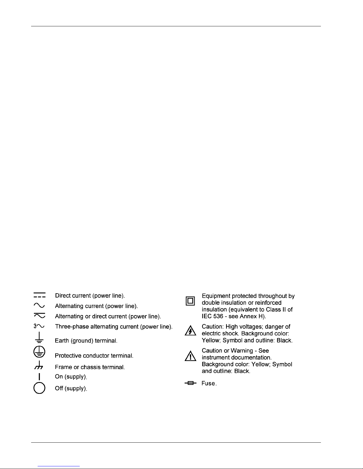
Lake Shore Model 340 Temperature Controller User’s Manual
3.1.3 Safety Summary
The following general safety precautions must be observed during all phases of operation, service, and repair
of this instrument. Failure to comply with these precautions or with specific warnings elsewhere in this manual
violates safety standards of design, manufacture, and intended use of the instrument. Lake Shore
Cryotronics, Inc. assumes no liability for Customer failure to comply with these requirements.
The Model 340 protects the operator and surrounding area from electric shock or burn, mechanical hazards,
excessive temperature, and spread of fire from the instrument. Environmental conditions outside of the
conditions below may pose a hazard to the operator and surrounding area.
• Temperature: 5 °C to 40 °C.
• Maximum relative humidity: 80% for temperature up to 31 °C decreasing linearly to 50% at 40 °C.
• Power supply voltage fluctuations not to exceed ±10% of the nominal voltage.
Ground the Instrument
To minimize shock hazard, the instrument chassis and cabinet must be connected to an electrical ground.
The instrument is equipped with a three-conductor AC power cable. The power cable must either be plugged
into an approved three-contact electrical outlet or used with a three-contact adapter with the grounding wire
(green) firmly connected to an electrical ground (safety ground) at the power outlet. The power jack and
mating plug of the power cable meet Underwriters Laboratories (UL) and International Electrotechnical
Commission (IEC) safety standards.
Do Not Operate in an Explosive Atmosphere
Do not operate the instrument in the presence of flammable gases or fumes. Operation of any electrical
instrument in such an environment constitutes a definite safety hazard.
Keep Away from Live Circuits
Operating personnel must not remove instrument covers. Component replacement and internal adjustments
must be made by qualified maintenance personnel. Do not replace components with power cable connected.
To avoid injuries, always disconnect power and discharge circuits before touching them.
Do Not Substitute Parts or Modify Instrument
Because of the danger of introducing additional hazards, do not install substitute parts or perform any
unauthorized modification to the instrument. Return the instrument to an authorized Lake Shore
representative for service and repair to ensure that safety features are maintained.
3.1.4 Safety Symbols
3-2 Installation
Page 39
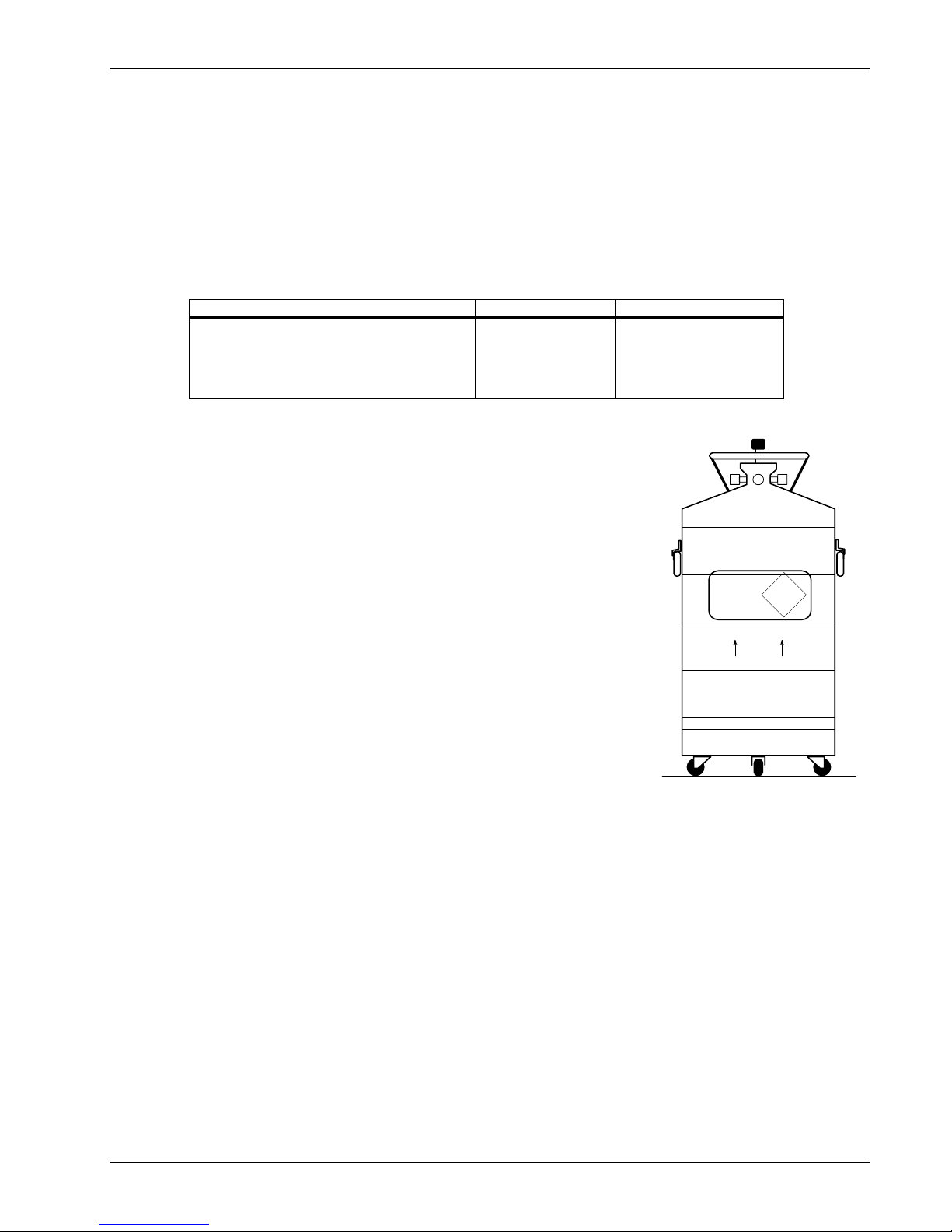
Lake Shore Model 340 Temperature Controller User’s Manual
3.1.5 Handling Liquid Helium and Liquid Nitrogen
Liquid Helium (LHe) and liquid nitrogen (LN
explosive, the following paragraphs provide safety considerations in the handling of LHe and LN
) may be used in conjunction with the Model 340. Although not
2
.
2
3.1.5.1 Properties
LHe and LN
are colorless, odorless, and tasteless gases. Gaseous nitrogen makes up about 78% of Earth’s
2
atmosphere, while helium comprises only about 5 ppm. Most helium is recovered from natural gas deposits.
Once collected and isolated, the gases liquefy when properly cooled. A quick comparison between LHe and
LN
is provided in Table 3-1.
2
Table 3-1. Comparison of Liquid Helium to Liquid Nitrogen
PROPERTY LIQUID HELIUM LIQUID NITROGEN
Boiling Point @1 atm, in K
Thermal Conductivity (Gas), w/cm–K
Latent Heat of Vaporization, Btu/liter
Liquid Density, pounds/liter
4.2
0.083
2.4
0.275
77.35
0.013
152
0.78
3.1.5.2 Handling Cryogenic Storage Dewars
All cryogenic containers (dewars) must be operated in accordance with
instructions from the manufacturer. Safety instructions are normally posted on
the side of each dewar. Cryogenic dewars must be kept in a well-ventilated
place where they are protected from the weather and away from any sources
of heat. A typical cryogenic dewar is shown in Figure 3-1.
3.1.5.3 Liquid Helium and Nitrogen Safety Precautions
Transferring LHe and LN
and operation of the storage dewar controls should
2
be in accordance with instructions from the manufacturer/supplier. During this
transfer, it is important that all safety precautions written on the storage dewar
MAGNETIC
LIQUID
HELIUM
NON-
NON-
FLAMMABLE
and recommended by the manufacturer be followed.
KEEP
WARNING
l Liquid helium and liquid nitrogen are potential asphyxiants and can
UPRIGHT
cause rapid suffocation without warning. Store and use in area with
adequate ventilation. DO NOT vent container in confined spaces. DO
NOT enter confined spaces where gas may be present unless area
has been well ventilated. If inhaled, remove to fresh air. If not
breathing, give artificial respiration. If breathing is difficult, give
oxygen. Get medical help.
l Liquid helium and liquid nitrogen can cause severe frostbite to the
eyes or skin. DO NOT touch frosted pipes or valves. In case of
frostbite, consult a physician at once. If a physician is not readily
Figure 3-1. Typical
Cryogenic Storage Dewar
available, warm the affected areas with water that is near body
temperature.
The two most important safety aspects to consider when handling LHe and LN2 are adequate ventilation and
eye and skin protection. Although helium and nitrogen gases are non-toxic, they are dangerous in that they
replace the air in a normal breathing atmosphere. Liquid products are of an even greater threat since a small
amount of liquid evaporates to create a large amount of gas. Therefore, it is imperative that cryogenic dewars
be stored, transfers accomplished, and systems operated in open and well ventilated areas.
Persons transferring LHe and LN
should make every effort to protect eyes and skin from accidental contact
2
with liquid or the cold gas issuing from it. Protect your eyes with full face shield or chemical splash goggles.
Safety glasses (even with side shields) are not adequate. Always wear special cryogenic gloves (Tempshield
Cryo-Gloves
®
or equivalent) when handling anything that is, or may have been, in contact with the liquid or
cold gas, or with cold pipes or equipment. Long sleeve shirts and cuffless trousers that are of sufficient length
to prevent liquid from entering the shoes are recommended.
Installation 3-3
Page 40

Lake Shore Model 340 Temperature Controller User’s Manual
3.1.5.4 Recommended First Aid
Every site that stores and uses LHe and LN
should have an appropriate Material Safety Data Sheet (MSDS)
2
present. The MSDS may be obtained from the manufacturer/distributor. The MSDS specifies the symptoms of
overexposure and the first aid to be used. A typical summary of these instructions is provided as follows.
If symptoms of asphyxia such as headache, drowsiness, dizziness, excitation, excess salivation, vomiting, or
unconsciousness are observed, remove the victim to fresh air. If breathing is difficult, give oxygen. If breathing
has stopped, give artificial respiration. Call a physician immediately.
If exposure to cryogenic liquids or cold gases occurs, restore tissue to normal body temperature (98.6 °F) as
rapidly as possible, then protect the injured tissue from further damage and infection. Call a physician
immediately. Rapid warming of the affected parts is best achieved by bathing it in warm water. The water
temperature should not exceed 105 °F (40 °C), and under no circumstances should the frozen part be
rubbed, either before or after rewarming. If the eyes are involved, flush them thoroughly with warm water for
at least 15 minutes. In case of massive exposure, remove clothing while showering with warm water. The
patient should not drink alcohol or smoke. Keep warm and rest. Call a physician immediately.
3.2 REAR PANEL DEFINITION
This paragraph provides a summary of Model 340 rear panel connections. See Figure 3-2.
CAUTION
l Verify that the AC Line Voltage shown in the window on the fuse holder corresponds to that
marked on the rear panel, and that both these settings are appropriate for the intended AC power
input. Also remove and verify the proper fuse is installed before inserting the power cord and
turning on the instrument.
l Always turn off the instrument before making any rear panel connections. This is especially critical
when making sensor to instrument connections.
120
-10% +5%
LINE 100 / 120
FUSE
50-60 Hz
DATA
190 VA MAX
DATA CARD
2.0 A
.25x1.25in T
220 / 240
1.0 A
IEEE-488 INTERFACE
5x25mm T
S
H1 AH1 T5 L4 SR1 RL1 PP0 DC1 DT0 C0 E1
11
HEATER FUSE
2.5 AMPS
WARNING
NO USER SERVICEABLE PARTS INSIDE. REFER
SERVICING TO TRAINED SERVICE PERSONNEL.
HEATER OUTPUT
SERIAL I/O
SHIELDLOHI
DIGITAL I/O
CAUTION: POWER OFF TO MATE PROBE
RELAYS
LO HI
NC C NO NC C NO
ANALOG
OUT 1
ANALOG
OUT 2
INPUT A INPUT B
l+V+l-
l+V+l-
V-
V-
1. Line Input Assembly ................................................. Paragraph 3.3
2. DATA CARD Slot...................................................... Paragraph 8.4
3. IEEE-488 INTERFACE Connector........................... Paragraph 9.1 and Figure 10-8
4. SERIAL I/O Connector ............................................. Paragraph 9.2 and Figure 10-2
5. DIGITAL I/O Connector ............................................ Paragraph 3.7 and Paragraph 7.2
6. RELAYS LO and HI Connector ................................ Paragraph 3.8
7. ANALOG OUT 1 and 2 Connectors ......................... Paragraph 3.6 and Paragraph 7.1
8. Sensor INPUT A and B Connectors......................... Paragraph 3.4
9. Option Cutout ........................................................... Paragraph 11.1
10. Loop 1 HEATER OUTPUT Banana Jacks ............... Paragraph 3.5
11. Loop 1 HEATER FUSE ............................................ Paragraph 3.5.4
Figure 3-2. Model 340 Rear Panel
3-4 Installation
Page 41

Lake Shore Model 340 Temperature Controller User’s Manual
3.3 LINE INPUT ASSEMBLY
The line input assembly contains the line
voltage selector, line fuse holder, and power
cord connector. It is important to verify that the
Model 340 is set to the appropriate line voltage
and has the correct line fuse before it is
powered on for the first time. Refer to Table 3-2.
If the final destination of the instrument is
known when it is shipped, the line input is
configured at the factory. This configuration
should always be checked because it is not
Indicator Line Voltage Range Fuse (slow blow)
Table 3-2. AC Line Input Definitions
100 90-105 VAC 2 A
120 108-126 VAC 2 A
220 198-231 VAC 1 A
240 216-252 VAC 1 A
unusual for an instrument to change hands before it reaches the end user. All of the line voltages discussed
are single phase.
Line voltage and fuse verification is discussed in Paragraph 3.3.1. Line voltage selection is discussed in
Paragraph 3.3.2. Fuse replacement is discussed in Paragraph 3.3.3. The power cord is discussed in
Paragraph 3.3.4. Finally, the power switch is discussed in Paragraph 3.3.5.
3.3.1 Line Voltage and Fuse Verification
To verify the proper line voltage selection look at the indicator in the window of the line input assembly. Line
voltage should be in the range shown in Table 3-1 for that indicator. If it is not, change the line voltage
selector as described in Paragraph 3.3.2. The fuse must be removed to verify its value. Refer to Paragraph
3.3.3 for fuse replacement instructions. Fuses are slow blow (time delay) type and should always be the value
specified in Table 3-1. Fuse values are also printed on the rear panel of the instrument for convenience.
WARNING: To avoid potentially lethal shocks, turn off controller and disconnect it from AC
power line before performing these procedures. Only qualified personnel should
perform these procedures.
CAUTION: For continued protection against fire hazard, replace only with the same type and
rating of fuse as specified for the line for the line voltage selected.
3.3.2 Line Voltage Selection
Below is the procedure to change the instrument line voltage selector. Verify the fuse value whenever line
voltage is changed.
1. Identify the line input assembly on the instrument rear panel.
2. Turn the line power switch OFF (O).
3. Remove the instrument power cord.
4. With a small screwdriver, release the drawer holding the line voltage selector and fuse.
5. Slide out the removable plastic fuse holder from the drawer.
6. Rotate the fuse holder until the proper voltage indicator shows through the window.
7. Verify the proper fuse value.
8. Re-assemble the line input assembly in the reverse order.
9. Verify the voltage indicator in the window of the line input assembly.
10. Connect the instrument power cord.
11. Turn the line power switch ON (l).
Installation 3-5
Page 42

Lake Shore Model 340 Temperature Controller User’s Manual
3.3.3 Fuse Replacement
Below is the procedure to remove and replace a line fuse. Use slow blow fuses with the value shown in
Table 3-1. To change line input from the factory setting, use the appropriate fuse in the connector kit shipped
with the instrument.
1. Locate the line input assembly on the instrument rear panel.
2. Turn the power switch OFF (O).
3. Remove the instrument power cord.
4. With a small screwdriver, release the drawer holding the line
voltage selector and fuse.
5. Remove fuse and replace it with the appropriate slow blow fuse.
6. Re-assemble the line input assembly in reverse order.
7. Verify voltage indicator in the line input assembly window.
8. Connect the instrument power cord.
Power On/Off
Swit ch
Screwdriver
Slot
Fuse
Draw er
Figure 3-3. Power Fuse Access
9. Turn the power switch ON (l).
3.3.4 Power Cord
The Model 340 includes a three-conductor power cord. Line voltage travels across the outer two conductors.
The center conductor is a safety ground and connects to the instrument metal chassis when the power cord
attaches to the power connector. For safety, plug the cord into an appropriate grounded receptacle.
3.3.5 Power Switch
The power switch turns the instrument ON and OFF and is located in the line input assembly on the
instrument rear. When l is raised on the switch, the instrument is ON; when O is raised, the instrument is
OFF. Do not remove instrument covers without first disconnecting the power cord, even if the instrument
power switch is off.
3.4 STANDARD SENSOR INPUTS
This paragraph details how to connect sensors to the standard Model 340 inputs. These inputs operate with
most resistive and diode sensors. Refer to Paragraph 5.1 to configure inputs for a sensor type with software.
Some sensor types require an optional input which is discussed in Chapter 10.
This section covers sensor input connector and pinout in Paragraph 3.4.1, sensor lead cable in Paragraph
3.4.2, grounding and shielding sensor leads in Paragraph 3.4.3, sensor polarity in Paragraph 3.4.4, four-lead
sensor measurement in Paragraph 3.4.5, two-lead sensor measurement in Paragraph 3.4.6, and lowering
measurement noise in Paragraph 3.4.7.
3.4.1 Sensor Input Connector and Pinout
The input connectors are 6-pin DIN 45322 sockets. The sensor output pins are defined in Table 3-3. Two
mating connectors (6-pin DIN plugs) are included in the connector kit shipped with the instrument. These are
common connectors, so additional mating connectors can be purchased from local electronics suppliers.
They can also be ordered from Lake Shore (P/N 106-233).
Table 3-3. Sensor INPUT A and B Connector Definition
Pin Symbol Description
1 I– Minus Current Terminal
2 V– Minus Voltage Terminal
INPUT A INPUT B
l+
l-
l+
l-
3 Shield Driven Shield or Guard
4 V+ Plus Voltage Terminal
5 I+ Plus Current Terminal
6 No Connection
V+
V-
V+
V-
3-6 Installation
Page 43

Lake Shore Model 340 Temperature Controller User’s Manual
3.4.2 Sensor Lead Cable
The sensor lead cable used outside the cooling system can be much different form what is used inside.
Between the instrument and vacuum shroud, error and noise pick up need to be minimized, not heat leak.
Larger conductor, 22 to 28 AWG stranded copper wire is recommended because it has low resistance yet
remains flexible when several wires are bundled in a cable. The arrangement of wires in a cable is also
important. For best results, voltage leads, V+ and V– should be twisted together and current leads I+ and I–
should be twisted together. The twisted pairs of voltage and current leads should then be covered with a
braided or foil shield which is connected to the driven shield pin of the instrument. This type of cable is
available through local electronics suppliers. Instrument specifications are given assuming 10 feet of sensor
cable. Longer cables, 100 feet or more, can be used but environmental conditions may degrade accuracy and
noise specifications.
3.4.3 Grounding and Shielding Sensor Leads
The sensor input measurements are isolated from earth ground to reduce the amount of earth ground
referenced noise that is present on the measurement leads. This isolation can be defeated by connecting
sensor leads to earth ground on the chassis of the instrument or in the cooling system. If one sensor lead
must be grounded, ground only one lead and ground it in only one place. Grounding leads on more than one
sensor prevents the sensor excitation current sources from operating.
Shielding the sensor lead cable is important to keep external noise from entering the measurement. A shield
is most effective when it is near the measurement potential so the Model 340 offers a driven shield that stays
close to the measurement. The shield of the sensor cable should be connected to the shield pin of the input
connector. It should not be terminated at the opposite end of the cable. The shield should not be connected to
earth ground on the instrument chassis or in the cooling system.
NOTE: The shell of the connector is in contact with the chassis so the cable shield should never
touch the outer shell of the connector.
The shield pin of the Model 340 input connector can be connected to the shield drive or the measurement
ground. The shield drive is recommended for cables over 20 feet in length. To change the shield pin contact,
use JMP6 for Input B and JMP5 for Input A. See Figure 11-11.
3.4.4 Sensor Polarity
Lake Shore sensors are shipped with instructions that indicate which
sensor leads are which. It is important to follow these instructions for
DT-470-SD
Diode Sensor Leads
plus and minus leads (polarity) as well as voltage and current when
applicable. Diode sensors do not operate in the wrong polarity. They
look like an open circuit to the instrument. Two lead resistors can
operate with any lead arrangement and the sensor instructions may
not specify. Four-lead resistors can be more dependent on lead
arrangement. Follow any specified lead assignment for four lead
resistors. Mixing leads could give a reading that appears correct but
is not the most accurate.
AnodeCathode
3.4.5 Four-Lead Sensor Measurement
All sensors, including both two lead and four lead can be
measured with a four lead technique. The purpose of a
four lead measurement is to eliminate the effect of lead
resistance on the measurement. If it is not taken out, lead
resistance is a direct error when measuring a resistive
sensor.
Four-Lead
Diode
I+
V+
V
I
V+
Four-Lead
Platinum
V
In a four lead measurement, current leads and voltage
leads are run separately up to the sensor. With separate leads there is little current in the voltage leads so
their resistance does not enter into the measurement. Resistance in the current leads will not change the
current as long as the voltage compliance of the current source is not reached. When two lead sensors are
used in four lead measurements, the short leads on the sensor have an insignificant resistance.
I+
I
Installation 3-7
Page 44

Lake Shore Model 340 Temperature Controller User’s Manual
3.4.6 Two-Lead Sensor Measurement
There are times when crowding in a cryogenic system forces users to
read sensors in a two lead configuration because there are not enough
feedthroughs or room for lead wires. If this is the case, plus voltage to
plus current and minus voltage to minus current leads are attached at the
back of the instrument or at the vacuum feedthrough.
The error in a resistive measurement is the resistance of the lead wire
Two-Lead
Diode
I+
V+
VI-
run with current and voltage together. If the leads contribute 2 or 3 Ω to a 10 kΩ reading, the error can
probably be tolerated. When measuring voltage for diode sensors the error in voltage can be calculated as
the lead resistance times the current, typically 10 µA. For example: a 10 Ω lead resistance times 10 µA
results in a 0.1 mV error in voltage. Given the sensitivity of a silicon diode at 4.2 K the error in temperature
would be only 3 mK. At 77 K the sensitivity of a silicon diode is lower so the error would be close to 50 mK.
Again, this may not be a problem for every user.
3.4.7 Lowering Measurement Noise
Good instrument hardware setup technique is one of the least expensive ways to reduce measurement noise.
The suggestions fall into two categories: (1) Do not let noise from the outside enter into the measurement,
and (2) Let the instrument isolation and other hardware features work to their best advantage.
• Use four lead measurement whenever possible.
• Do not connect sensor leads to chassis or earth ground.
• If sensor leads must be grounded, ground leads on only one sensor.
• Use twisted shielded cable outside the cooling system.
• Attach the shield pin on the sensor connector to the cable shield.
• Do not attach the cable shield at the other end of the cable, not even to ground.
• Run different inputs and outputs in their own shielded cable.
• Use twisted wire inside the cooling system.
• Use similar technique for heater leads.
• Use a grounded receptacle for the instrument power cord.
• Consider ground strapping the instrument chassis to other instruments or computers.
3.5 HEATER OUTPUT SETUP
The following paragraphs cover the heater wiring from the vacuum shroud to the instrument for both control
loop outputs. Software settings and limit configuration of the heater output are detailed in Paragraph 6.12.1.
For information on choosing and installing an appropriate resistive heater, refer to the Paragraph 2.4.
Loop 1 output is discussed in Paragraph 3.5.1. Heater output connector for Loop 1 is discussed in Paragraph
3.5.2. Heater output wiring for Loop 1 is discussed in Paragraph 3.5.3. Heater protection and fuse for loop is
discussed in Paragraph 3.5.4. Noise on Loop 1 heater leads is discussed in Paragraph 3.5.5. The Lake Shore
Model 3003 Heater Output Conditioner is discussed in Paragraph 3.5.6. The Loop 2 output is discussed in
Paragraph 3.5.7. Loop 2 output resistance is discussed in Paragraph 3.5.8. The Loop 2 output connector is
discussed in Paragraph 3.5.9. Loop 2 heater protection is discussed in Paragraph 3.5.10. Finally, boosting the
output power is discussed in Paragraph 3.5.11.
3.5.1 Loop 1 Output
The Model 340 has two control loops. Loop 1 can be considered a primary loop because it is capable of
driving 100 W of heater power. The heater output for Loop 1 is a traditional control output for a cryogenic
temperature controller. It is a variable DC current source with several software settable ranges and limits.
The maximum heater output current is 2 A and maximum compliance voltage is 50 V.
3.5.2 Heater Output Connector for Loop 1
A dual banana jack on the rear panel of the instrument is used for connecting wires to the Loop 1 heater. A
standard dual banana plug mating connector is included in the connector kit shipped with the instrument. This
is a common jack and additional mating connectors can be purchased from local electronic suppliers. They
can also be purchased from Lake Shore (P/N 106-009).
3-8 Installation
Page 45

Lake Shore Model 340 Temperature Controller User’s Manual
3.5.3 Heater Output Wiring for Loop 1
Heater output current is what determines the size (gauge) of wire needed to connect the heater. The
maximum current that can be sourced from the Loop 1 heater output is 2 A. When less current is needed to
power a cooling system it can be limited in software with range settings. The load can be protected against
catastrophic instrument failure with heater fuse described below.
When setting up a temperature control system it is recommended that the lead wire for the heater be capable
of carrying a continuous current that is greater than the maximum current or heater fuse rating. Wire
manufactures recommend 26 AWG or larger wire to carry 2 A of current, but there is little advantage in using
wire smaller than 20 to 22 AWG.
It is recommended to use twisted, shielded cable for heater leads. Large changes in heater current can
induce noise in measurement leads and twisting reduces the effect. It is also recommended to run heater
leads in a separate cable from the measurement leads to further reduce interaction. There is a chassis
ground point at the rear panel of the instrument for shielding the heater cable. The cable shield can be tied to
this point with a single banana plug. The shield should not be connected at the opposite end of the cable.
The Loop 1 heater output is isolated from chassis ground to reduce noise. For best noise performance, do not
connect the resistive heater or its leads to ground. Also avoid connection heater leads to sensor leads or any
other instrument inputs or outputs.
3.5.4 Heater Protection and Fuse for Loop 1
The heater output of the Model 340 is a current source and has protection that prevents it from being
damaged even if shorted. The heater fuse on the rear panel of the instrument is there to provide one more
level of protection for delicate cooling systems. A fuse is a current limiting device, it burns out if too much
current is passed through it. Some systems require little heater power which requires only a small amount of
current. Even though the Model 340 has software current limits, the user may wish to put a smaller fuse into
the heater fuse holder to protect against inadvertent changes in instrument settings.
The heater fuse is shipped from the factory with a 2.5 A, ¼ × 1¼ inch fuse. This fuse can be replaced with a
value less than 2.5 A but should never be replaced with a higher value.
3.5.5 Loop 1 Heater Noise
The heater output circuitry in the Model 340 must be capable of sourcing 100 W of power. This type of
circuitry can generate some excess electrical noise. The Model 340 was designed to generate as little noise
as possible but even noise that is a small percentage of the output voltage or current can be too much when
sensitive measurements are being made near by. If the Model 340 heater leads are too noisy and the above
wiring techniques do not help, Lake Shore offers the Model 3003 Heater Output Conditioner that may help.
3.5.6 Model 3003 Heater Output Conditioner
The Lake Shore Model 3003 heater output conditioner is a passive filter which reduces the already low noise
present in the heater output of the Model 340. The Model 3003 connects between the heater output terminals
on the rear panel of a controller and a resistive heater. See Figure 3-4. Specifications are as follows:
Max Current: 2 A
Max Voltage: 60 V
Attenuation: 50 or 60 Hz. (line frequency): 20 dB
100 Hz. and above (line frequency harmonics): 40 dB
Size: 144 mm wide × 72 mm long × 165 mm deep (5.7 × 2.8 × 6.5 inches)
Weight: 1.6 kilograms (3.5 pounds)
Installation 3-9
Page 46

Lake Shore Model 340 Temperature Controller User’s Manual
The Model 3003 is a passive filter and requires no
external power supply. The High and Low terminals
on the controller must be connected to the High and
Low terminals marked From Controller on the Model
3003. The binding posts or a dual banana plug can
be used to connect to the model 3003. Precautions
must be taken to ensure the High and Low terminals
FROM CONTROLLER
CAUTION:
THIS HI TERMINAL
MUST BE
HI
CONNECTED TO
HI TERMINAL OF
THE CONTROLLER
LO
TO HEATER
HI
LO
are not reversed. A diode in the Model 3003 shorts
the heater output if the polarity of the terminals is
reversed.
The High and Low terminals marked To Heater on
Figure 3-4. Model 3003 Heater Output Conditioner
3003 Heater Output Conditioner
the Model 3003 should be attached to a resistive
heater used for temperature control. The binding
posts or a dual banana plug can be used to connect to the Model 3003. The ground terminals on the
Model 3003 continue the shield if the heater cable is shielded.
3.5.7 Loop 2 Output
The Model 340 has a second control loop called Loop 2. Loop 2 is an auxiliary control loop with enough
features to control a radiation shield or small sample heater. Loop 2 has a different output from Loop 1, it uses
Analog Output 2 as its actuator. It is a variable DC voltage source that can vary from -10 V to +10 V. The
resolution of the analog output is 1.25 mV or 0.0125% of full scale. The output can source up to 100 mA of
current providing a maximum of 1 W of heater power.
3.5.8 Loop 2 Output Resistance
2
The power delivered by the Loop 2 output is calculated as:
V
P
=
R
heater
The output is rated for no more than 100 mA of current, so for the maximum of 1 W output power use a 100 Ω
resistive heater with a power rating greater than 1 W. Smaller resistance values should not be used, but
larger resistances can be used for lower power applications.
3.5.9 Loop 2 Output Connector
The connector for Loop 2 output, which is Analog Output 2, is a BNC connector. The inner conductor is the
output voltage terminal, the outer conductor is attached to chassis ground inside the instrument. A coaxial
cable with attached BNC terminal is recommended for this output. The center conductor is capable of carrying
the maximum current and the outer conductor acts as a shield. It is not recommended to attach the outer
conductor to ground at the opposite end of the cable. These connectors are not included with the Model 340
but is available from local electronic suppliers.
3.5.10 Loop 2 Heater Protection
The output is short protected so the instrument is not harmed if the heater resistance is too small. It is not
recommended because the additional load on instrument power supplies causes noise on internal circuits.
The second control loop has fewer features than the first including software protection and limits. The user
must be careful to build a robust system and account for the voltage range and power up state of the control
output.
3-10 Installation
Page 47

Lake Shore Model 340 Temperature Controller User’s Manual
3.5.11 Boosting the Output Power
There are temperature control systems that require more power than the Model 340 can provide. An auxiliary
DC power supply can be used to boost the output of the Model 340. Programmable power supplies are
available that use a low current programming voltage as an input to control a high current voltage output.
Analog output 2, used for Loop 2 output, provides an ideal programming voltage for an auxiliary power supply.
The only drawback with using the analog output to program auxiliary supplies is it only has one voltage range.
The heater output for Loop 1 has several ranges that can improve resolution, but its output is in current not
voltage. A programming resistor can be placed across the heater output to produce a programming voltage.
The programming voltage is related to output current by:
VRI
program program output
=×
The resistor must be chosen to convert a full scale current from the highest heater output range being used to
the full scale programming voltage of the auxiliary supply. For example, it the auxiliary supply has a full scale
programming voltage of 10 V and the maximum current for the highest heater output range being used is 0.25
A the programming resistor should be 10 V / 0.25 A = 40 Ω. The programming resistor must be rated for the
power being dissipated in it which is
Power I R
=×
2
output program
or 2.5 W. Lower heater output current ranges
can be selected to reduce the power dissipated in the programming resistor.
3.6 ANALOG OUTPUTS
Analog Output 1 and Analog Output 2 on the rear panel of the
Model 340 are voltage outputs that can be used for monitor and
control applications. See Figure 3-5. Their most basic function
is a temperature monitor where they put out a voltage that is
proportional to temperature. They can be configured to monitor
the output of a linear equation which allows the user to select
an offset and gain. ANALOG OUT 2 can be used as the control
output for Loop 2. The analog outputs can also be controlled
manually by the user for any application that requires a
programmable voltage source.
Both analog outputs are variable DC voltage sources that can
PIN DESCRIPTION
vary from -10 V to +10 V. The resolution of the analog output
is 1.25 mV or 0.0125% of full scale. The output can source up
to 100 mA of current providing a maximum of 1 W of power.
They can drive a resistive load of no less than 100 Ω. The
output is short protected so the instrument is not harmed if the
heater resistance is too small. It is not recommended because
1
Analog Output, Center Conductor
2
Ground, Connector Shell
Figure 3-5. ANALOG OUT 1 and 2
BNC Rear Panel Connector Details
the additional load on instrument power supplies causes noise on internal circuits.
The connectors for the analog outputs are BNC sockets. The inner conductor is the output voltage terminal,
the outer conductor is the outputs ground and is attached to chassis ground inside the instrument. A coaxial
cable with attached BNC plug is recommended for this output. These connectors are not included with the
Model 340 but is available from local electronic suppliers.
It is not recommended to attach the analog output ground to a ground outside the instrument. The output
should be read by an instrument with an isolated or differential input wherever possible. Connecting to an
external ground can cause noise in the analog output voltage or the sensor input measurement. If this cannot
be avoided, try to keep the chassis of the two instruments at the same potential with a ground strap.
Installation 3-11
Page 48
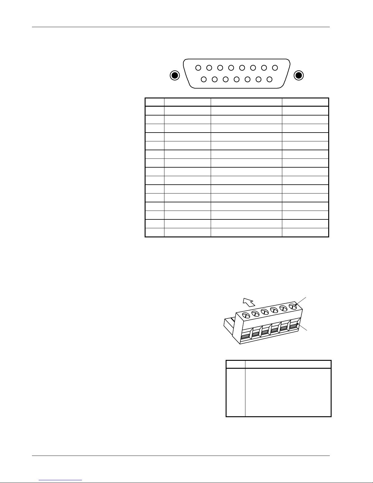
Lake Shore Model 340 Temperature Controller User’s Manual
3.7 DIGITAL I/O
The connector labeled Digital I/O on the
rear panel of the Model 340 has terminal
pins with digital inputs and outputs along
876
DIGITAL I/O
54321
with power supplies. See Figure 3-6.
The digital inputs and outputs can be
used to in applications that involve
15 14 13 12
11 10 9
auxiliary sensor input scanners. These
signals can also be used in manual
mode to control and monitor external
events. The power supplies are
provided for external circuit
applications that require low current.
The digital inputs and outputs are
Transistor-to-Transistor Logic (TTL)
voltage level compatible. They are
protected against short circuit and over
voltage, but it is not recommended to
expose the terminals to electrostatic
discharge (ESD), voltages higher than
5 volts, or lower than ground. Using
more current than the limits in Figure
3-6 is not recommended because the
additional load on instrument power
supplies causes noise on internal
circuits. All signals and power supplies
should be returned to the ground pin
whenever possible. Even though the
ground pin is connected to chassis
ground inside the Model 340, attaching
the ground pin to external grounds can
Pin Symbol Description Type or Limit
1 DO1 Digital Output 1 TTL Output
2 DO2 Digital Output 2 TTL Output
3 DO3 Digital Output 3 TTL Output
4 DO4 Digital Output 4 TTL Output
5 DO5 Digital Output 5 TTL Output
6 Reserved/DI6 Acting as Digital Input 6 TTL Input
7 +5 V +5 Volts Output 100 mA max
8 +15 V +5 Volts Output 50 mA max
9 DI1 Digital Input 1 TTL Input
10 DI2 Digital Input 2 TTL Input
11 DI3 Digital Input 3 TTL Input
12 DI4 Digital Input 4 TTL Input
13 DI5 Digital Input 5 TTL Input
14 -15 V -15 Volt Output 50 mA max
15 Gnd Ground -
Figure 3-6. DIGITAL I/O DA-15 Rear Panel Connector Details
cause noise on the sensor input measurements.
The connector is a 15 pin D-style socket. This is a common socket (P/N 268-303) and mating plug
(P/N 268-301) can be purchased from Lake Shore or any local electronic supplier.
3.8 RELAYS
The Model 340 has one high and one low relay, shown in
Figure 3-7. They are most commonly associated with the
alarm feature. The relays can also be put in manual
mode and controlled directly by the user from the front
panel or over computer interface. Refer to Paragraph
7.4. The relay status indicated on the relays and beeper
screen is for monitoring the relay status. It can not be set
by the user. If a relay is inactive (Off), it will be in its
normal state of open or closed. When the relay is active
Slides into RELAYS slot
Screw Terminal
Connector
Lake Shore
P/N 106-737
in rear of Model 340
1
6
5
4
3
2
Use
screwdriver
to lock or
unlock wires
Insert wire
into slot
(On), it will be in the opposite state.
The relay outputs have a detachable 6-pin terminal block connector.
The connector can be removed from its socket for convenient
installation of wires. The connector is included with the Model 340
(P/N 106-737). The connector manufacturer indicates that up to 12
AWG stranded copper wire can be used with the connector. It is
unlikely that wire that large will be required to carry the rated 2 amp
current of the relay.
3-12 Installation
PIN DESCRIPTION
1
Low, Normally Closed (N.C.)
2
Low, Common
3
Low, Normally Open (N.O.)
4
High, Normally Closed (N.C.)
5
High, Common
6
High, Normally Open (N.O.)
Figure 3-7 RELAYS LO and HI
Rear Panel Connector Details
Page 49

Lake Shore Model 340 Temperature Controller User’s Manual
CHAPTER 4
FRONT PANEL OPERATION
4.0 GENERAL
This chapter covers turning power on in Paragraph 4.1, display formats in Paragraph 4.2, keyboard
description in Paragraph 4.3, keypad navigation in Paragraph 4.4, and changing display format in
Paragraph 4.5. Be sure to read Paragraph 3.3 on line voltage verification before proceeding.
4.1 TURNING POWER ON
Once the line voltage setting has been verified (Paragraph 3.3), plug the instrument end of the line cord
(included in the connector kit) into the back of the instrument. Then plug the opposite end of the cord into a
properly grounded, three-prong receptacle. Place the power switch, located next to the line cord connector, to
the On position. The display backlight will brighten the display area and a Lake Shore graphic logo will appear
on the display. The alarm beeper will sound once and the instrument will show a display of sensor readings
and control settings.
There are several types of feedback that may be present at this time. Some indicate a problem with the
instrument and others indicate the need for the user to setup the sensor inputs or control loops. Problems are
indicated by the following:
• The display backlight does not turn on (backlight is dim indicating a cold instrument).
• The display does not show a logo or change from the logo.
• An error window appears with a message about a hardware problem. Refer to Paragraph 11.9.
• The alarm beeper does not sound.
• Instrument does not respond to keys being pressed.
If any of these symptoms are observed, please contact the factory.
Messages that indicate the need for further setup are common when first powering up the unit because many
users do not have temperature sensors installed or sensor type selected. Do not be concerned if the following
appear: overload condition, no sensor attached, no temperature response curve selected, or words
indicating a problem with the heater configuration in the area of the display that normally shows heater output.
These problems will be resolved as instrument setup is completed.
LakeShore
340 Temperature Controller
340-1-1.eps
4.2 DISPLAY FORMATS
The Model 340 has an eight line by 40 character LCD graphic display capable of showing small (6
large (12 × 16) characters. This display is very flexible and provides the user feedback at each step of
operation. The normal display of the Model 340 shows sensor readings and control status. Other specialized
displays are used for instrument settings, data entry, help and error messages.
The normal display is discussed in Paragraph 4.2.1. Setting displays is discussed in Paragraph 4.2.2. Data
entry displays are discussed in Paragraph 4.2.3. Finally, error displays are discussed in Paragraph 4.2.4.
Front Panel Operation 4-1
Auto
Zone
Ramp
Manual
Output
Pro gr am
Control
D
Setup
Loop 1
Loop 2
Tune
Settings
PI
Control
Heater
Range
Channel
Heater
Setpoint
Off
Figure 4-1. Model 340 Front Panel
Input
Setup
Scan
Setup
Alarm
Setup
Alarm
Reset
Display
SoftCal
Format
789
Curve
Inte r f a ce
Ent r y
456
Analog
Math
Outputs
Setup
123
Math
Options
Reset
0
+/-
.
+/-
Cance l
Escape
Sc r e en M o r e
Previous
Setting
Loca l
Next
DataCard
Setting
Save
Ent er
Help
Sc r e en
× 8) and
Page 50

Lake Shore Model 340 Temperature Controller User’s Manual
4.2.1 Normal Display
The normal display is what the instrument shows
under normal operating conditions, when the user is
not changing a setting, and there is not a hardware
failure detected. The top line of the display is
dedicated to showing instrument status. Status
annunciators appear on the top line when applicable.
Annunciators that may be seen include: Tune,
A
+1. 0 0 3 3 8
A
86.084
Loop 1 Channel A
Setp +0.00000 V
Heat Disabled
Normal Display with Both Loops Shown
B
V
K
+0 . 9995 6
B
88.020
Loop 2 Channel A
Setp +0.00000 V
Output
Logging, Program, Ramping, Alarm, Remote,
and Locked.
The next four lines are used to show sensor input
readings. This area is configurable by the user to
show between one and eight readings. From one to
four readings can be shown in large characters, five
to eight readings are shown using smaller characters.
A
+1.00338
A
86.084
Loop 1 Channel A
Setp +0.00000 V
Heat Disabled
Normal Display with One Loop Shown
B
V
K
+0 . 999 56
B
88.020
P 0.0
I 0.0 MOut
D 0.0 100.00%
V
K
The bottom three lines show control settings and status. This area is configurable to show information from
one or two control loops. If one loop is being displayed, the heater output can be shown in large characters.
Some examples of normal display configurations are shown here. Instructions on how to change the display
configuration are provided in the following paragraphs.
4.2.2 Setting Displays
Users may enter common parameters like control setpoint directly from the normal display. Other instrument
setup parameters have unique setting displays that conveniently combine several related parameters on one
screen. For details, refer to Paragraph 4.4 – Keypad Navigation.
V
K
4.2.3 Data Entry Displays
Data entry displays are special setting displays. Their layout allows easy entry of data tables including
temperature response curves. They follow the same instructions as setting displays in Paragraph 4.4 –
Keypad Navigation.
4.2.4 Error Displays
Some error conditions are part of normal operation and do not prevent the instrument from operating. Error
messages for these will be shown on the normal display and the instrument will continue to operate until the
situation is corrected. Errors that prevent the instrument from functioning properly can result in an error
display that replaces the normal display. In this case the instrument will not try to operate until the error has
been corrected. Error messages are summarized in Paragraph 11.9.
Some errors result from mistakes made when changing instrument settings or entering data. If this happens,
read and follow the instructions shown. Also verify the settings by going back to the setting screen after the
instrument has shown a normal display.
4.3 KEYPAD DESCRIPTION
The Model 340 has 40 keys on its keypad which help prompt the operator in using the large number of
powerful software features. This section will help the user understand the keypad layout and how to quickly
get to the features of interest.
The Model 340 keypad is divided into three groups. The group of 16 keys near the display are used for
temperature control features. The middle group of 16 keys has two functions. The key tops are labeled with
numbers and symbols for number entry. Above these keys are labels for temperature measurement, display
and interface features. The last group of 8 keys is used for navigating in setting screens and has a few spare
keys for features that the operator may need quickly.
4-2 Front Panel Operation
Page 51

Keypad Description (Continued)
Lake Shore Model 340 Temperature Controller User’s Manual
Aside from the key location, the color of the panel behind the key is also important. Direct settings, made with
the normal display showing, are initiated using keys with a gray background. The number keys and the gray
backed Enter, Escape, up (s), or down (t) keys are used to complete these operations when needed.
The keys with a white background initiate a setting screen. One or more associated parameters are grouped
on the setting screen. The white backed Next Setting, Previous Setting, Save Screen, Cancel Screen, and
More keys are used to move around within setting screens. Once the desired parameter is highlighted, it can
be set with the number entry keys. Examples are given below in keypad navigation.
4.4 KEYPAD NAVIGATION
This section gives specifics on how to set desired parameters. Number entry and setting selection are
discussed first because these operations are needed for both direct settings and setting screens.
4.4.1 Changing Parameters
After highlighting the desired parameter, use the middle group of keys to enter a new value into the
highlighted field. Press Enter to end data entry and accept the new value. Press Escape to end data entry
and restore the old value. Press Help to view limits and resolution for most parameters.
NOTE: Within setting screens, press Save Screen to accept the entire screen. Press Cancel Screen
or let the keypad time-out to return the screen parameters to pre-setting values.
Use the s or t key to toggle an On/Off or Yes/No toggle or select from a list of possible parameter settings.
Enter accepts the new setting and Escape restores the old setting.
4.4.2 Direct Settings
To save the operator time, the most commonly used
parameters can be set directly from the normal
display screen. These keys are located in the area
of the front panel with a gray background.
Some direct functions happen immediately when
the key is pressed. These include the Heater Off,
Loop 1, Loop 2, Alarm Reset, Math Reset, and
Local keys. No other keys are required to complete
these operations.
Pressing other keys with a gray background will
highlight the parameter indicated on the key. The
parameter can then be set by entering a number or
selecting a setting. P, I, D, Manual Output and
Setpoint values are entered as numbers. Heater
Range and Control Channel are set with s or t key
from a list of settings. Then press the Enter key to
accept or Escape key to cancel.
A
+1. 0 0 3 3 8
A
86.084
Loop 1 Channel A
Setp +0.00000 V
Heat Disabled
Normal Display with Control Channel Highlighted
A
+1. 0 0 3 3 8
A
86.084
Loop 1 Channel A
Setp +0.00000 V
Heat Disabled
Normal Display with Temperature Setpoint Highlighted
B
V
K
V
K
+0 . 999 56
B
88.020
P 0.0
I 0.0 MOut
D 0.0 100.00%
B
+0 . 999 56
B
88.020
P 0.0
I 0.0 MOut
D 0.0 100.00%
V
K
V
K
Front Panel Operation 4-3
Page 52
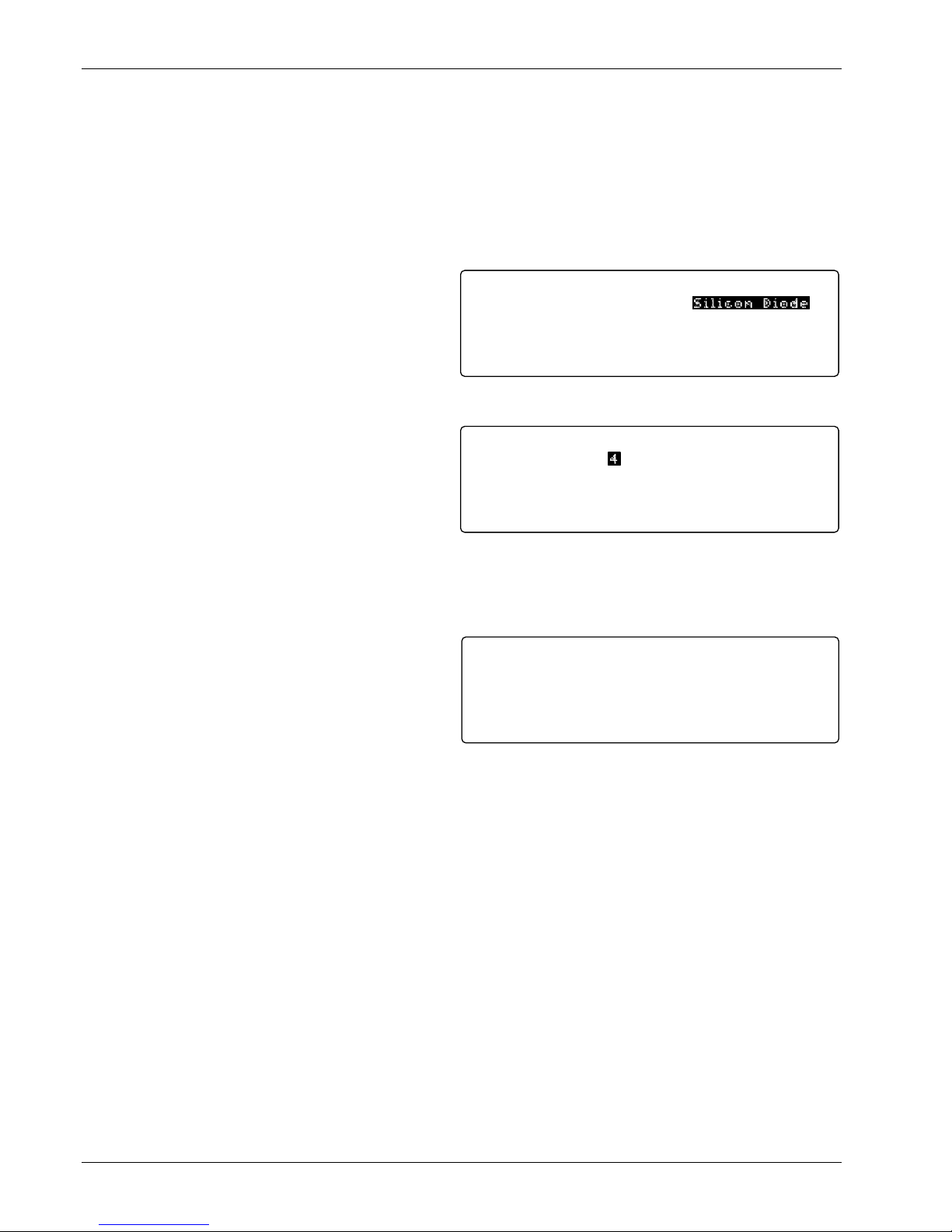
Lake Shore Model 340 Temperature Controller User’s Manual
4.4.3 Using Setting Screens
Use setting screens to change less used parameters. Press keys with a white background to display the
parameter setting screen associated with that key. The setting screen title displays on the center of the top
line.
On screens that contain parameters associated with sensor inputs or control loops, the top left corner will
show the sensor input or control loop. This field must be set correctly before proceeding. Use the s or t key
to select the appropriate sensor input or control loop and then press enter. The correct parameters will then
be shown on the setting screen.
The Next Setting and Previous Setting keys are
used to move around within the setting screen.
Once a parameter has been chosen and it is
highlighted, the data entry discussed above should
be used to make changes. The Next Setting and
Previous Setting keys will act like the Enter key
and end the setting operation.
Input: A INPUT SETUP
Type: Silic on Diode
Sensor Unit:
Curve:
SN:
1 D T -4 7 0
Standard
Temp Coeff:
Excitation:
Entering a New Sensor Type for Input A
Range:
V
Neg.
10 u A
§2.5V
After making changes to a screen, press Save
Screen to store the changes into the Model 340.
Press Cancel Screen or let the keypad time-out to
return screen parameters to pre-setting values.
A <more> annunciator may appear in the right
Input Displays:
Disp1:
Disp3:
A SENSOR
A TEMP K
Disp2:
Disp4:
A SENSOR
A TEMP K
<more>READING DISPLAY FORMAT
corner of the screen to indicate that the parameters
would not fit on one screen. Other parameters will
be shown if the More key is pressed. If the More
Example screen showing <more>
key is pressed after changes are made to a screen,
a message prompts users to save or ignore the settings.
4.4.4 Data Entry Screens
Data entry screens are similar to setting screens, but
they have data tables that are too long to fit on a
screen. Scroll up and down the data table instead of
using the More key to change screens. In the
following example of entering a temperature
response curve, curve identification information is
entered like a setting screen then the curve data is
Name:
Limit:
Format:
Coeff:
Edit Curve: # 1
DT-470
SN:
Sta ndard
499.900
V/K
Neg.
(I) In s e r t
Sensor Temp(K)
1:
0.09062 475.000
2:
0.10191 470.000
3:
0.11356 465.000
4:
0.12547 460.000
5:
0.13759 455.000
(D ) D e le t e
Entering a Temperature Response Curve
entered in a long table.
4.4.5 The Help Key
The Help key at the lower right corner of the keypad can be pressed while selecting a parameter. The
information shown on the display will tell the operator the intended use of the parameter, then if the More key
is pressed, the setting limits and resolution of the parameter. Next the help will show how to use the
navigation keys discussed above as a reminder. Pressing Cancel Screen or the Help key will return the
instrument to its setting operation. Pressing Help from the normal display shows how to use the navigation
keys.
4.4.6 Keypad Time-out
The Model 340 suspends some of its operation during keypad operation. (The control loop and computer
interfaces are never disabled.) A time-out was put in the keypad so that the instrument would return to normal
operation if a key happened to be unintentionally pressed. The time-out acts like an Escape or Cancel
Screen key being pressed so that no accidental changes are made to settings. Even with the time-out, we do
not recommend you do long data entry operations while the instrument controls an experiment.
4-4 Front Panel Operation
Page 53

4.4.7 Key Definitions
Key Description
AutoTune
Zone Settings
Ramp
Program
P
I
D
Control Setup
Heater Range
Heater Off
Control Channel
Loop 1
Loop 2
Setpoint
Manual Output
Input Setup
SoftCal
Display Format
Scan Setup
Curve Entry
Interface
Alarm Setup
Math Setup
Analog Outputs
Alarm Reset
Math Reset
Options
Displays the AUTO TUNE screen to set Auto P, Auto PI, or Auto PID control mode.
Displays the ZONE SETTINGS screen which specifies P, I, D, Manual Output, and
Heater Range for up to 10 Temperature control zones.
Displays the RAMP SETUP screen which turns ramp on or off and selects ramp rate.
Displays the PROGRAM MODE screen. Allows the user to Run an internal program,
Terminate a program, Edit a program, or Clear program memory.
Allows direct setting of the proportional (P) control parameter.
Allows direct setting of the integral (I) control parameter.
Allows direct setting of the derivative (D) control parameter.
Displays the CONTROL SETUP screen which enables the control loop, establishes
power up status and setpoint units, sets heater resistance and control mode, and turns
the filter on or off. Press the More key to display the CONTROL LIMITS screen which
sets the temperature, slope, maximum heater current, and range.
Allows direct setting of Loop 1 heater range.
Immediately turns off Loop 1 heater.
Allows direct setting of the sensor feedback channel for a control loop.
Displays Control Loop 1 parameters and status on lower three lines of display.
Displays Control Loop 2 parameters and status on lower three lines of display.
Allows direct setting of control setpoint.
Allows direct setting of manual output control parameter.
Displays the INPUT SETUP screen which selects the sensor type and curve number.
Other sensor parameters can be overwritten, but this changes sensor status to
"Special." Only curves appropriate to the sensor type display.
Displays the SOFTCAL screen which accepts and stores SoftCal curves.
Displays three screens (use the More key to toggle between the screens):
1. The READING DISPLAY FORMAT screen sets the number of readings (1 thru 8)
2. The CONTROL DISPLAY FORMAT screen sets lower three lines of the display.
3. The MISC. DISPLAY FORMAT screen sets display contrast, back lighting, and
Displays the EXTERNAL SCANNER SETUP screen to set external scanner support.
Displays the CURVE ENTRY screen which edits, copies, or erases temperature
response curves.
Displays the COMPUTER INTERFACE screen which sets IEEE-488.2 and Serial
interface parameters.
Displays the ALARM SETTINGS screen which enables or disables alarms and sets
various alarm parameters.
Displays the MATH COMPUTATIONS screen which sets Max/Min and Filter
parameters. Press the More key to see the LINEAR EQUATION screen.
Displays the ANALOG OUTPUTS screen which specifies Mode, Bipolar, Status, and
other parameters for Analog Output A and B.
Immediately resets all latched alarms.
Immediately resets all Max and Min values.
Displays four screens:
1. The DIGITAL I/O screen manually sets the digital inputs and outputs.
2. The RELAY & BEEPER SETUP screen allows the user to choose alarm or manual
3. The DATE & TIME screen is used to set real-time clock.
4. The REVISION INFORMATION screen displays the controller serial number and
Use the More key to toggle between the screens.
Lake Shore Model 340 Temperature Controller User’s Manual
shown in the normal display and assigns an input and data source to each.
keypad lock.
control for relays and to turn the beeper on or off.
revision history.
Front Panel Operation 4-5
Page 54

Key Definitions (Continued)
Key Description
Escape
Up (s)
Down (t)
Enter
Cancel Screen
Previous Screen
Next Setting
Save Screen
More
Local
Data Card
Help
Lake Shore Model 340 Temperature Controller User’s Manual
Return a parameter to its original value during parameter entry.
Toggle a parameter or selects a setting from a list.
Toggle a parameter or selects a setting from a list.
Completes the operation of setting a value during parameter entry.
Returns parameters in a setting screen to pre-setting values.
Moves to the previous parameter location within a setting screen.
Moves to the next parameter location within a setting screen..
Saves new parameter values in a setting screen.
Shows additional parameters that do not fit on one setting screen.
Toggles the IEEE-488.2 Interface between remote and local modes.
Displays the DATACARD screen. Allows the user to select Data Logging,
Read DataCard, Write DataCard, and Erase DataCard. Datacards are useful
for transferring temperature response curves, storing and restoring instrument
parameters and internal programs, and updating main processor software.
Displays a help screen for the highlighted parameter.
4.5 CHANGING DISPLAY FORMAT
The Model 340 lets the user decide which information is shown on the display. This section discusses the
display fields that can be configured using the Display Format key.
4.5.1 Number of Readings Displayed
The Model 340 can display between one and eight input readings at a time. If one to four readings are
chosen, they will be shown with the large characters. If five to eight readings are chosen, they will be shown
with small characters.
To change the number of display readings, press the Display Format key. You will see the Reading Display
Format screen with the current number of Input Displays highlighted. Use a number key or the s or t key
to select the desired number of reading displays, then press the Enter key. The lower portion of the setting
display will now show the available display fields ready for the operator to enter a sensor input and reading
source. The default setting is 2.
4.5.2 Sensor Input
The Model 340 has two sensor inputs, A and B. More sensor input can be added with Model 340 options.
Input A can be used to monitor more than one sensor with the use of an external scanner. Scanner support is
covered in Paragraph 5.4.
To select a sensor input for a display field, press the Display Format key. You will see the Display Format
screen with the current number of Input Displays highlighted. Use the Enter or Next Setting key to select
the display number, then use the s or t key to select the desired input. Then press the Enter key. A sensor
input can appear in as many reading fields as desired. The default setting is A and B.
4-6 Front Panel Operation
Page 55
Lake Shore Model 340 Temperature Controller User’s Manual
4.5.3 Reading Source and Display Units
Readings shown on the display are taken from the sensor inputs, but a variety of digital processing can be
done to the raw sensor data before it is displayed (see Figure 5-10). One or more of these sources can be
displayed at the same time for an active sensor input.
Sensor
Raw sensor units as read from the temperature sensor.
Temp K Temperature in Kelvin. Requires a temperature response curve selected
in Input Setup. Refer to Paragraph 5.1.
Temp C Temperature in Celsius. Requires a temperature response curve selected
in Input Setup. Refer to Paragraph 5.1.
Max
Min
Linear
Maximum value read since last reset. Refer to Paragraph 5.3.2.
Minimum value read since last reset. Refer to Paragraph 5.3.2.
Output of a linear equation. Refer to Paragraph 5.3.3.
To select a display reading source, enter the sensor input (above). Press the Enter key to highlight the field
next to the input. use the s or t key to select a source for that reading display from the list. If a temperature
source is selected and no temperature response curve is present an error message will appear on the normal
display (NOCURV). Press the Enter or Next Setting key to change the next reading display. Press the Save
Screen key to store the changes in the Model 340. The default setting is Temp K.
4.5.4 Control Loop Display
The Model 340 has the ability to operate one or two temperature control loops. The user has the option of
displaying parameters from either one or both loops. When both loops are displayed, fewer parameters are
shown on the normal display. The hidden parameters can be viewed by pressing the Loop 1 or Loop 2 key,
they will also appear when being changed.
Loop 1
Loop 2
Displays Loop 1 parameters including P, I, D and Manual Out
Displays Loop 2 parameters including P, I, D and Manual Out
Both Displays setpoint, control channel, and percent (%) output for both loops,
Heater Range for Loop 1.
None
Neither set of control loop parameters are shown.
To select a control loop display format, press the Display Format key, then press the More key to show the
CONTROL DISPLAY FORMAT screen. The control loops line will be highlighted so use the s or t key to
select one of the choices. Press the Enter or Next Setting key to continue with other settings. Press the
Save Screen key to store the changes in the Model 340. The default setting is Loop 1.
4.5.5 Large Heater Display
There are applications where the amount of power being driven into the control load is as important as the
control temperature. In this case the control loop output can be shown in large characters on the display. The
larger output will replace P, I, D, and Manual Output on the display. The hidden parameters will still appear
when being changed.
To turn the large output display on or off, press the Display Format key, then press the More key until you
see the CONTROL DISPLAY FORMAT screen. Press the Next Setting key until the Large Output line is
highlighted, then use the s or t key to select on or off. Press the Enter or Next Setting key to continue with
other settings. Press the Save Screen key to store the changes in the Model 340. The default setting is Off.
NOTE: The Large Output option will not be visible if Control Loops: BOTH is selected. Change the
Control Loop setting back to Loop 1 or Loop 2, press the Enter key, then the Large Output
selection will be available.
Front Panel Operation 4-7
Page 56

Lake Shore Model 340 Temperature Controller User’s Manual
4.5.6 Heater Output Display Units
The CONTROL DISPLAY FORMAT screen is also the place to select whether heater output is shown as
POWER or CURRENT. This setting will impact the heater output seen in the normal display and which units
are used for the manual output (MOut) display. If current is selected, the heater output and range will appear
as 20% @ 100 W to indicate 20% output current for the selected 100 watt range. If power is selected for the
same output, the heater output and range would appear as 4% of 100W to indicate 4% output power for the
selected 100 watt range.
To change the heater display units, press the Display Format key, then press the More key until you see the
CONTROL DISPLAY FORMAT screen. Press the Next Setting key until the Heat Display line is highlighted,
then use the s or t key to select Current or Power. Press the Enter or Next Setting key to continue with
other settings. Press the Save Screen key to store the changes. The default setting is Current.
4.5.7 Display Contrast
The Model 340 has a high contrast, LCD display with a bright backlight. The factory contrast setting is good
for most applications, but it will need to be changed for arrangements of equipment that put the Model 340
well above or below eye level. Display contrast can be set to a value between 0 an 100. Please note that
changing contrast has no effect on the display backlight.
To change display contrast, press the Display Format key then press the More key until the Misc. Display
Format screen is displayed. Press the Next Setting key until the Contrast line is highlighted, then use the
s or t key to adjust contrast. The contrast will change as the parameter is being set, so adjustments should
be made with the operator and instrument in their normal positions. Press the Enter or Next Setting key to
continue with other settings. Press the Save Screen key to store the changes in the Model 340. The default
setting is 50.
4.5.8 Display Backlight On/Off
The Model 340 display used a florescent tube as a backlight. The backlight is powered with a high voltage
supply operating at 30 kHz. Some experiments are sensitive to noise in the frequency range of 30 kHz, so the
backlight power supply can be turned off. Please note that the display is unreadable when the backlight is off.
To turn the display backlight off, press the Display Format key, then press the More key to show the MISC.
DISPLAY FORMAT screen. Press the Next Setting key until the line for backlight is highlighted, then use the
s or t key to turn the backlight off. Press the Save Screen key to store the changes. Default setting is On.
To turn the display backlight back on, press any key on the keypad.
4.5.9 Locking the Keypad
The Model 340 has a keypad lock feature to prevent accidental changes to instrument parameters and
minimize the disturbances of curious onlookers. A simple 3 number sequence is the code needed to lock and
unlock the keypad. The factory default code is 123
and it can only be changed using a computer interface.
To lock or unlock the keypad, press the Display Format key then press the More key to show the Misc.
Display Format screen. Press the Next Setting key until Lock is highlighted, then use the s or t key to
toggle the lock setting. Press the Enter key. A small setting window will appear for entering a three digit
number code. Use the number keys to enter the code, then press the Enter key. Press the Save Screen key
to store the lock status in the Model 340. The default setting is unlocked, code 123
.
When the keypad is locked, you can still see values for the various parameters, you just cannot change them.
The only front panel keys that are active when the keypad is locked are the Heater Off and Alarm Reset keys.
4.6 DEFAULT VALUES
It is sometimes necessary to reset instrument parameters to their factory default values. These values can be
cleared without affecting instrument calibration.
To reset the Model 340 parameters to factory default values, press the Options key then press the More key
until the Revision Information screen is displayed. Up the s or t key to change the Set Defaults setting to
Yes, then press the Enter key. Press the Save Screen key to complete the action. The Model 340 will then
restart using the factory default values.
4-8 Front Panel Operation
Page 57
Lake Shore Model 340 Temperature Controller User’s Manual
CHAPTER 5
SENSOR INPUT AND
TEMPERATURE MEASUREMENT OPERATION
5.0 GENERAL
This chapter describes front panel operation for sensor input configuration and temperature measurement.
The user must setup temperature sensor input before a valid sensor reading can be made, and select a
temperature response curve to convert readings to temperature. This chapter covers sensor input setup in
Paragraph 5.1, selecting a temperature response curve in Paragraph 5.2, filter and math functions in
Paragraph 5.3, and scanner support in Paragraph 5.4.
5.1 SENSOR INPUT SETUP
This section covers sensor type in Paragraph 5.1.1, voltage excitation in Paragraph 5.1.2, thermal
EMF compensation with voltage excitation in Paragraph 5.1.3, special sensor type configuration in
Paragraph 5.1.4, and turning an input off in Paragraph 5.1.5.
5.1.1 Sensor Type
The first step in sensor input configuration is setting the sensor type parameter. The Model 340 works with
a variety of different sensors, each with special requirements for excitation and input range. Selections for
several different types of sensors are pre-programmed into the Model 340. If using one of these sensor types,
select that type to automatically change the associated parameters listed in Table 5-1.
Table 5-1. Sensor Types Recognized by the Model 340
Type Units Excitation Range Temp. Coefficient Update
Silicon Diode volts 10 µA 0-2.5 V Negative 20 Hz
GaAlAs Diode volts 10 µA 0-7.5 V Negative 20 Hz
Platinum 100/250 ohms 1 mA
Platinum 100/500 ohms 1 mA
Platinum 1000 ohms 100 µA
Rhodium-Iron ohms 1 mA
*Carbon-Glass ohms 10 mV
*Cernox ohms 10 mV
*Ruthenium Oxide ohms 10 mV
*Germanium ohms 1 mV
* Refer to Paragraph 5.1.2 for voltage excitation for these sensors. Approximate temperature ranges are given
with specifications. Other sensor types are available with input option cards.
0-250 Ω
0-500 Ω
0-2500 Ω
0-250 Ω
0-300 kΩ
0-300 kΩ
0-300 kΩ
0-30 kΩ
To select a pre-programmed sensor type, press Input Setup. The input setup setting screen appears with the
input letter in the top left hand corner. Use the s or t key to select an input. Press Enter or Next Setting to
display the input parameters. Press Next Setting until the type field highlights and then use the s or t key to
select one of the sensor types in the table above. Press Enter or Next Setting to show the input parameters
for that sensor type. To proceed to temperature response curve selection (Paragraph 5.2), press Previous
Setting or press Save Screen to store the changes in the Model 340. The default setting is Silicon Diode.
NOTE: If the user changes any of the parameters listed for a standard sensor type, the
instrument assumes a special sensor type is required (Paragraph 5.1.4).
NOTE: Use the display setup screen (Paragraph 4.5) to show configured readings from an input
on the display.
Positive 20 Hz
Positive 20 Hz
Positive 20 Hz
Positive 20 Hz
Negative 10 Hz
Negative 10 Hz
Negative 10 Hz
Negative 10 Hz
Measurement Operation 5-1
Page 58

Lake Shore Model 340 Temperature Controller User’s Manual
5.1.2 Voltage Excitation (Current Autorange)
Several RTD sensor types have a nonlinear temperature response. These sensors require special excitation
so that their signal can be read with good resolution and at the same time not too much power is dissipated in
the sensor. When these sensors are being read by the Model 340, the current excitation is automatically
ranged to keep the voltage across the sensor below that listed in the table above. To illustrate the effect,
power can be expressed by either:
2
2
× R or P
P = I
V
=
.
R
Using these negative temperature coefficient resistors with resistance (R) and a constant current (I)
excitation, the power in the sensor will increase as temperature drops (resistance increases), but with
constant voltage (V) excitation, the power reduces as temperature drops.
Voltage excitation is indicated for several sensors in the table above that should be read using low power.
Other than using an autoranging current source, voltage excitation often requires compensation for thermal
EMF that is described below. Note that thermal compensation will reduce the update rate of these inputs from
20 readings per second to 10 readings per second.
5.1.3 Thermal EMF Compensation with Voltage Excitation
Sensors that require voltage excitation must be operated with little power dissipated in the sensor. To keep
power low, the voltage across the sensor is kept low. There are two major problems that occur when
measuring small DC voltages. The first is external noise entering the measurement through the sensor leads
which is discussed with sensor setup. The second problem is the presence of thermal EMF voltages,
sometimes called thermocouple voltages, in the lead wiring. Thermal EMF voltages appear whenever there is
a temperature gradient across a piece of voltage lead. They can be canceled in the measurement with a
similar temperature gradient in the other voltage lead. Thermal EMF voltages must exist because the sensor
is almost never the same temperature as the instrument. They can be minimized by careful wiring, making
sure the voltage leads are symmetrical in the type of metal used and how they are joined, and by keeping
unnecessary heat sources away from the leads. Even in a well designed system thermal EMF voltages can
be an appreciable part of a low voltage sensor measurement.
The Model 340 can help with a thermal correction algorithm. The instrument will automatically reverse the
polarity of the current source every other reading. The average of the positive and negative sensor readings
will cancel the thermal EMF voltage which is present in the same polarity, regardless of current direction. The
settling time associated with current reversal will reduce the update rate of a corrected input from 20 readings
per second to 10 readings per second.
Thermal correction can be turned off, but it is not recommended because reading errors will increase. The
default setting is ON. Thermal correction can also be paused for a short time. This feature is useful when the
temperature system is stable and the user wants to make delicate experimental measurements with little
disturbance entering the system. The Reverse setting is for diagnostic purposes only. Thermal correction
parameter field will appear on the input setup screen when a sensor type using voltage excitation is selected.
To change the thermal correction parameter to on, off or pause, press the Input Setup key. The input setup
setting screen will appear with the Input letter in the top left hand corner. Use the s or t key to select an
input. Press the Enter key or the Next Setting key to display the input parameters for that input. Press the
Next Setting key until the thermal compensation field is highlighted and then use the s or t key to select on,
off or pause. Press the Next Setting key to continue with more settings or press the Save Screen key to
store the changes in the Model 340. The default setting is On.
5.1.4 Special Sensor Type Configuration
The Model 340 allows sensors that do not match a pre-programmed type. Configure input excitation and input
range selections to meet specific needs. Users may set the temperature coefficient to allow a specially
configured input as a control channel, display units in volts or ohms, and create and select a response curve
for the special input or use a linear equation to compensate for the raw reading.
The Model 340 pre-programmed settings do not include every combination of excitation and input range.
Setting combinations not included in pre-programmed conditions do not have published specifications. The
user must determine input configuration suitability for their application.
5-2 Measurement Operation
Page 59

Lake Shore Model 340 Temperature Controller User’s Manual
Table 5-2. Special Sensor Type Configuration
Excitation Input Range Temperature Coefficient Units
1 mA
300 µA
100 µA
30 µA
10 µA
3 µA
1 µA
300 nA
100 nA
30 nA
*10 mV
*1 mV
5 V
2.5 V
1 V
500 mV
250 mV
100 mV
50 mV
25 mV
10 mV
5 mV
2.5 mV
1 mV
Positive
Negative
Volts
Ohms
The columns in the above table can be selected independently. When voltage units are selected the input
range is as listed in the table. When resistance units are selected, resistance range can be computed as
R = V/I. Again, it is up to the user to determine the suitability of a special input configuration. Input
configurations that indicate a resistance range of more than 1 MΩ are not recommended because the
instrument itself will begin to cause measurement errors.
To select a special sensor type, press the Input Setup key. The input setup setting screen will appear with
the input letter in the top left hand corner. Use the s or t key to select an input. Press the Enter key or the
Next Setting key to display the input parameters for that input. Press the Next Setting key until the type field
is highlighted and then use s or t key to select special from the list of settings. Press the Enter key or the
Next Setting key and to advance to the next parameter. Set the parameters of units, temperature coefficient,
excitation and input range from the list in the table above. If special setup was successful, proceed to
temperature response curve selection in Paragraph 5.2 by pressing the Previous Setting key or press the
Save Screen key to store the changes in the Model 340.
5.1.5 Turning an Input Off
There are cases, particularly when using scanned inputs, that the user may wish to turn off an input. This can
be done from the input setup screen. If an input that has been turned off is chosen for the display, the
DISABLE message will appear in the reading field.
To turn an input off, press the Input Setup key. The INPUT SETUP screen will appear with the input letter in
the top left hand corner. Use the s or t key to select input A or B. Press the Enter or Next Setting key until
the Enable field is highlighted. Use the s or t key to select OFF. Press the Save Screen key to store the
change in the Model 340.
5.2 SELECTING A TEMPERATURE RESPONSE CURVE
A temperature response curve is needed to convert a sensor reading in sensor units to temperature. A curve
is a table of breakpoints, each containing a temperature value and its sensor units equivalent for the sensor.
The section on sensor selection discusses different ways of obtaining temperature response curves. Curves
can also be created by the user and entered into the instrument as described in the curve entry section. It is
assumed that an appropriate curve is present in the Model 340 before proceeding with this section.
Some types of sensors behave in a predictable manner and a standard temperature response curve can be
created for them. The Model 340 has standard curves included in firmware. Refer to Table 5-3. Details on
standard curves are provided in Appendix B.
Curves entered by the user or loaded as CalCurves will appear during curve selection list. They will have
curve number 21 to 60. The sensor serial number will appear on the setting screen and can be used to
identify a unique curve if the serial number was included with the curve table.
NOTE: During curve selection, the instrument may only show the curves that are appropriate for an
input type. It is necessary to select an appropriate input type before selecting a curve. Refer to
Paragraph 5.4 for a description of how to select multiple curves for a scanned input.
Measurement Operation 5-3
Page 60

Lake Shore Model 340 Temperature Controller User’s Manual
To select a temperature response curve, press the Input Setup key. The input setup setting screen will
appear with the input letter in the top left hand corner. Use the s or t key to select an input. Press the Enter
key or the Next Setting key to display the input parameters for that input. Press the Next Setting key until
the curve field is highlighted and then use s or t key to select a curve from the list. Press the Enter key or
the Next Setting key and to advance to the next parameter. (If curve selection was not successful, press the
Next Setting key and verify the appropriate type selection). Press the Save Screen key to store the changes
in the Model 340.
Table 5-3. Standard Curve Table
Curve Setting No. Sensor Type Model Number Curve Name Temp. Range Table
DT-470 1 Silicon Diode DT-470 Curve 10 1.4 – 475 K A-1
DT-500-D 2 Silicon Diode *DT-500-DRC-D Curve D 1.4 – 365 K
DT-500-E1 3 Silicon Diode *DT-500/DRC-E1 Curve E1 1.4 – 330 K
PT-100 4 Platinum RTD 100 PT-100 DIN 43760 30 – 800 K
PT-1000 5 Platinum RTD 1000 *PT-1000 DIN 43760 30 – 800 K
Type K 6 Thermocouple Type K Type K
Type E 7 Thermocouple Type E Type E
3.15 – 864 K (1500 K
3.15 – 622 K (930 K
A-2
A-3
†
)
A-4
†
)
A-5
Type T 8 Thermocouple Type T Type T 3.15 – 670 K A-6
AuFe .03% 9 Thermocouple Chromel-AuFe 0.03% Chromel-AuFe 0.03% 3.50 – 500 K A-7
AuFe .07% 10 Thermocouple Chromel-AuFe 0.07% Chromel-AuFe 0.07% 3.15 – 610 K A-8
DT-670 11 Silicon Diode DT-670 DT-670 1.4 – 500 K A-9
* Curves supported but sensors no longer available through Lake Shore.
†
Temperature range extended when using ±50 mV Range.
5.3 FILTER AND MATH
Some simple arithmetic features have been included in the Model 340 as a convenience to the user. Filter,
Max, Min and linear equation can be applied to an input reading. As shown in Figure 5-1, the filter can be
applied to all readings for an input. The results of Max, Min, and linear equation can be shown on the display
in combination with the actual input reading. The display format screen is used to configure the display.
5.3.1 Filter
The Model 340 can apply an averaging filter to any sensor input. The filter is designed to prevent electronic
noise that is picked up on the sensor lead wires from showing on the display. It is enabled or disabled for all
of the reading formats of an input at the same time. A number of readings filtered and filter reset window can
be changed by the user to meet their application. The control equation has a filter that is enabled
independently from the input filter.
To turn on the filter for an input, press the Math
Setup key. The MATH COMPUTATIONS screen
appears with the Input field highlighted. Use the
s or t key to select an input. Use the Enter or
Next Setting key to move the cursor to FILTER
Input: A
MAX/MIN FILTER
Enable:
Source:
ON
TEMP K
Enable:
Points:
Window:
<more>MATH SETUP
ON
10
1%
Enable. Use the s or t key to select ON. The
default setting is On.
The user may change filter behavior by changing the number filter readings. Although more filter readings
settle the display reading more, it is not always appropriate to select many filter readings. More filter readings
also slow display reading response to real temperature changes in the load.
To change on the filter readings (points) for an input, press the Math Setup key. You see the MATH
COMPUTATIONS screen. The Input field is highlighted. Use the s or t key to select an Input. Use the
Enter or Next Setting key to move the cursor to FILTER Points. Use the s or t key to select the desired
number. The minimum number of points is 2, the maximum is 64. The default setting is 10.
Some users do not want the filter to slow the response of the display reading when large deliberate changes
in temperature are made. The filter window parameter allows the user to set the limit for a large temperature
change. If an unfiltered reading differs from the filtered reading by more than the filter window limit, the filter
will be restarted. The filter window limit is set in percent of full scale range for the selected input type.
To change the filter window for an input, press the Math Setup key. You will see the MATH
COMPUTATIONS screen. The Input field will be highlighted. Use the s or t key to select an Input. Use the
Enter or Next Setting key to move the cursor to FILTER Window. Use the s or t key to select the desired
percentage. The minimum is 1%, the maximum is 10%. The default setting is 1%.
5-4 Measurement Operation
Page 61
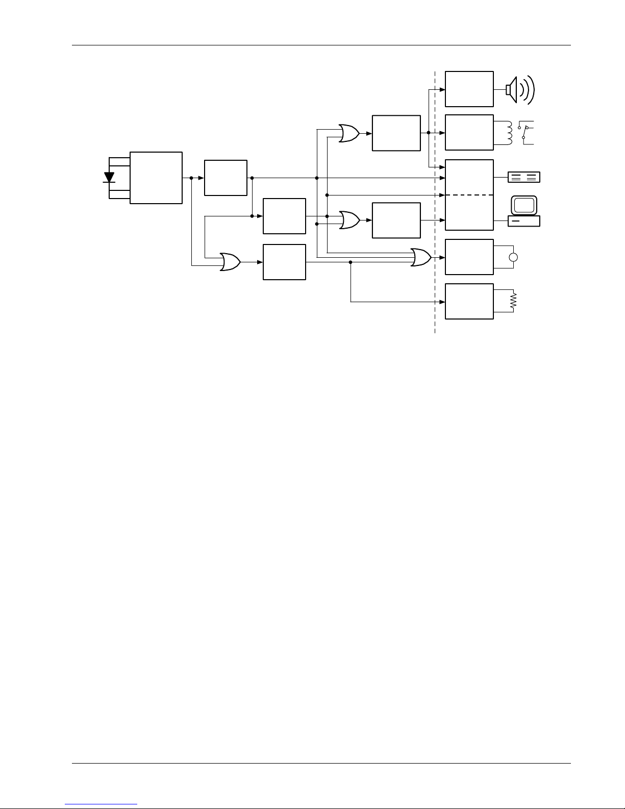
Lake Shore Model 340 Temperature Controller User’s Manual
Beeper
OR
Alarms
Relays
Input
Processing
Conversion
to Temperature
Filter
OR
Linear
Equation
PID
Control
OR
Maxim um/
Minimum
OR
Display
Remote
Analog
Out
V
Heater
Out
340-5-1.eps
Software
Hardware
Figure 5-1. Data Flow
5.3.2 Max/Min
The Model 340 will save the highest (Max) and lowest (Min) reading of a sensor input when the Max/Min
feature is turned on. The feature can be paused to save these stored values after the observation period is
over. A source for Max/Min must be selected on the math setup screen. There are four possible sources for
the Max/Min feature. The input reading in sensor units, kelvin, Celsius, or the result of the linear equation can
be chosen. Max/Min will work with one source for an input but different inputs can have different sources. Max
and Min will not automatically show on the display. Use the Reading Display Format screen described in
Paragraph 4.5 to show Max and Min on the display.
To use the Max/Min feature, press the Math Setup key. The math setting screen will appear with the input
letter in the top left hand corner. Use the s or t key to select an input. Press the Enter key or the Next
Setting key to display the Max/Min parameters for that input. Press the Next Setting key until the Max/Min
enable field is highlighted and then use s or t key to select on. Press the Next Setting key or the Enter key
to advance to the source field. Use the s or t key to select one of the four sources. Press the Next Setting
key to make other changes. Press the Save Screen key to store the change in the Model 340. The default
settings are On, kelvin.
When the Max./Min feature is setup, it will not automatically appear on the display. Use the display format
screen to add a reading field to the display and select the input and math source for that new field. Display
format is discussed in Paragraph 4.5.
To Pause the Max/Min feature, press the Math Setup key. The math setting screen will appear with the input
letter in the top left hand corner. Use the s or t key to select an input. Press the Enter key or the Next
Setting key to display the Max/Min parameters for that input. Press the Next Setting key until the Max/Min
enable field is highlighted and then use s or t key to select pause. Press the Save Screen key to store the
change in the Model 340. Changing back and fourth between on and pause will not reset the values.
To reset the Max/Min values, press the Math Reset key from the normal display. Math reset is an immediate
operation.
Measurement Operation 5-5
Page 62

Lake Shore Model 340 Temperature Controller User’s Manual
5.3.3 Linear Equation
The Model 340 can calculate a linear equation as a special data processing feature. The output of this
calculation can be shown on the display or directed to an analog output for proportional control of other
hardware in an experiment. One computation can be done for each sensor input. The output will not
automatically show on the display, use the display format setting screen described in Paragraph 4.5 to
change display settings. If an analog output is being used, its output scale must be set (Paragraph 7.1).
There are two different equations available. In each: M is a gain or slope, X is an input reading, and B is an
offset or intercept (not to be confused with input B). The two equations are shown in the table below. The
difference between them is subtle. The first equation is used to scale the raw reading of an input, similar to a
temperature response curve, when the sensor has linear response. The second is better at generating a
control signal when a setpoint (SP1 or SP2) is selected as B. The control signal can then be directed to an
analog output. The second equation is also useful whenever a reading of deviation from setpoint is needed.
The columns settings in Table 5-4 are selected
independently. “Number” represents a number entered by
Table 5-4. Linear Equation Configuration
the user. “X” can be set to an input reading in sensor
units or temperature in kelvin or Celsius. SP1 represents
setpoint of Loop 1 and similarly for other B settings.
To setup a linear equation, press the Math Setup key
and the math setting screen will appear. Press the More
key to show the setting screen for linear equation with
the input letter in the top left hand corner. Use the s or
Equation M X B
MX+B
M(X+B)
Number Sensor
Temp K
Temp C
Number
SP1
–SP1
SP2
–SP2
t key to select an input. Press the Enter key or the Next Setting key to display the equation parameters for
that input. Use the s or t key to select one of the two equations from the highlighted equation field. Press
the Next Setting key and continue to select parameter settings for M, X, and B. A number setting field will
appear next to the field for B if number is selected from the B setting list. The scale factor can be selected as
n, µ, m, k, M, or G. Blank indicates a scale factory of x1. Press the Save Screen key to store the change in
the Model 340. The default settings are M(X+B), 1, K, –SP1.
5.4 SCANNER SUPPORT
The Model 340 supports a user-supplied sensor scanner (external to the instrument). Scan up to 16 sensors
of the same type into input A. The sensors must be the same type because only one sensor type setting can
be made for the A input. Each of the 16 sensors (channels) can have a unique temperature response curve.
There are different modes of scan operation that allow for active scan channel selection. If a channel is not
actively read, the last valid reading for that channel either displays or reports over the computer interface.
Four-lead sensor measurement is always recommended when scanning temperature sensors.
5.4.1 Scan Modes
Scanner support has different modes for selecting which of the channels is actively being read. Each mode
allows for a different scanner applications.
Manual
Auto Scan
Slave
Off
To select a scanner support mode, press the Scan
The user manually selects the scan channel over front panel or computer interface.
Digital outputs report the scanned channel if set to scanner mode.
The instrument sequences through enabled channels, holding on each channel for a
user-specified interval. Digital outputs report the scanned channel if set to scanner mode.
The external scanner selects the channel through the digital inputs
All scan functions are disabled.
EXTERNAL SCANNER SETUP
Setup key. The Mode field will be highlighted. Use
the s or t key to select the appropriate scan mode.
Then press the Save Screen key. The default
setting is Off.
Mode:
5-6 Measurement Operation
Page 63

Lake Shore Model 340 Temperature Controller User’s Manual
5.4.2 Input Setup with a Scan Mode Active
When any of the scan modes are selected, the input setup screen for the A input will change slightly. The
input field will allow setting of channel A1 thru A16 and a temperature response curve can be entered for each
channel. Changing parameters other than enable and curve will act globally for all channels.
To select a scan channel for setup, press the Input Setup key. Use the s or t key to select input A. Press
the Enter key. The scan channel number will be highlighted. Use the s or t key to select the desired scan
channel number (1 thru 16). Press the Enter key. The Enable field is now highlighted. Use the s or t key to
select ON. Press the Enter key. The Curve field is now highlighted. Use the s or t key to select the desired
sensor to temperature curve (only curves appropriate to the sensor type display). Press the Save Screen key.
The default settings are Channel 1 and Enable On.
Once the channels are setup and enabled, use Display Format to actually display the results of the scan
channels on the front panel. Refer to Paragraph 4.5.
5.4.3 Manual Scanning
Once the individual input channels have a designated curve, the user can manually select the channel to be
scanned. The Model 340 can set its digital outputs to the corresponding scan channel. If the external scanner
has digital control inputs the Model 340 can be used to select a channel. This is a convenient way to
synchronize the scanned readings or automate the scan operation using only the interface of the Model 340.
To manually select a scan channel for reading,
EXTERNAL SCANNER SETUP
press the Scan Setup key. The Mode field will be
highlighted. Use the s or t key to select
MANUAL. Press the Enter key. The Channel
selector will appear. Use the s or t key to select
Channel:
Mode:
A1
MANUAL
the appropriate channel and press the Save
Screen key to store the change in the Model 340.
The default setting is A1.
The digital outputs must be set to scan mode to
report the scan channel. Refer to Paragraph 7.2 for
digital output mode setting. When the digital
outputs are set to work with the scanner and
manual scan mode selected, digital output signals
D1 to D4 report the active scan channel as shown
below. Digital output logic levels are described in
Paragraph 7.2.
Channel DO4 DO3 DO2 DO1
1 0 0 0 0
2 0 0 0 1
3 0 0 1 0
4 0 0 1 1
5 0 1 0 0
6 0 1 0 1
7 0 1 1 0
8 0 1 1 1
9 1 0 0 0
10 1 0 0 1
11 1 0 1 0
12 1 1 1 1
13 1 1 0 0
14 1 1 0 1
15 1 1 1 0
16 1 1 1 1
Measurement Operation 5-7
Page 64
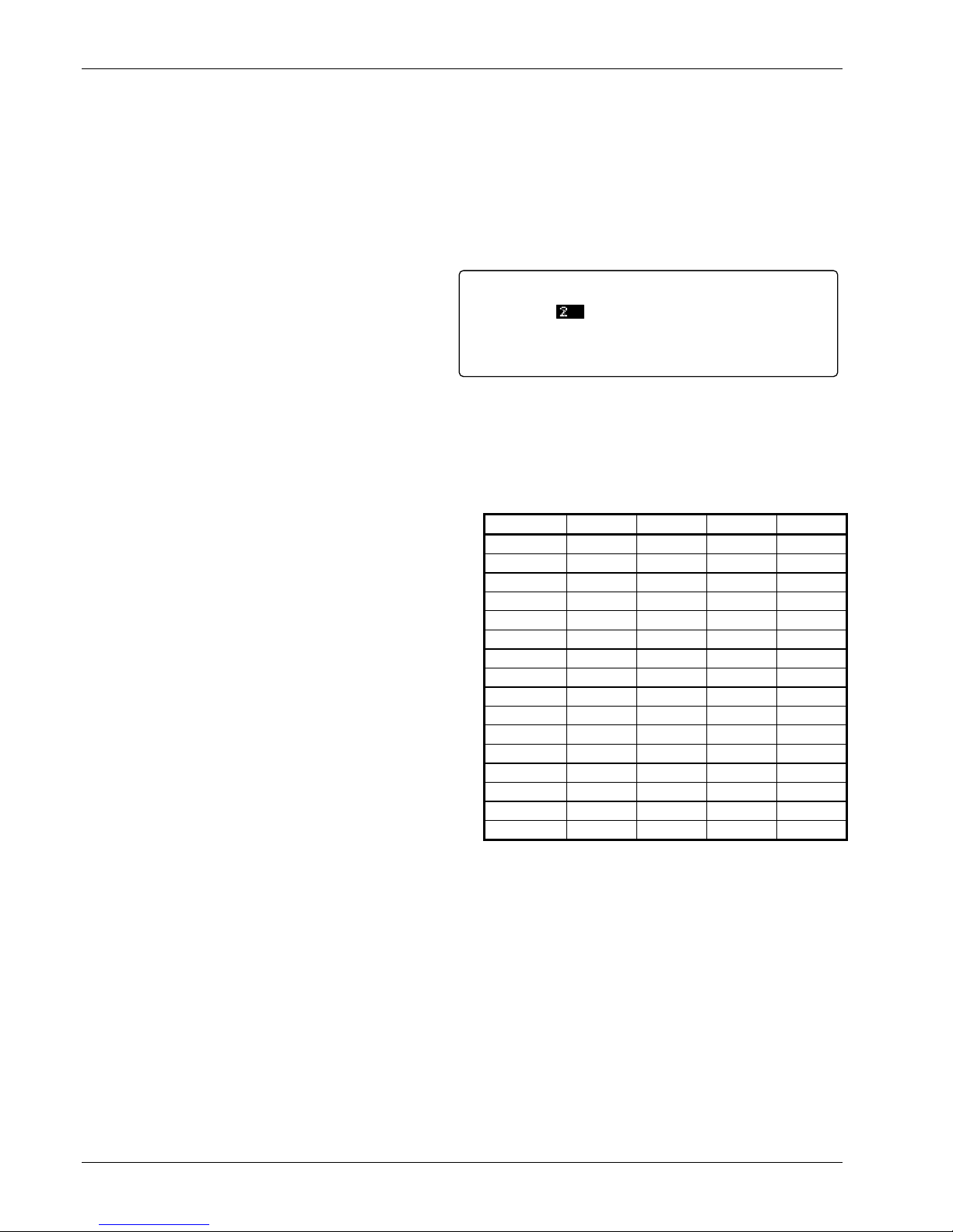
Lake Shore Model 340 Temperature Controller User’s Manual
5.4.4 Auto Scanning
Once the individual input channels are enabled and have a designated curve, the Auto Scan feature can
sequence through the enabled channels. A scan interval can be set by the user to tell the instrument how long
to read a channel before moving to the next. The interval is set in seconds and has a range of 2 to 200. The
Model 340 can set its digital outputs to the corresponding Auto Scan channel. If the external scanner has
digital control inputs the Model 340 can be used to select a channel. This is a convenient way to synchronize
the scanned readings or automate the scan operation using only Model 340.
To change the reading interval for the Auto Scan
mode, start with the scan mode set to Auto Scan.
EXTERNAL SCANNER SETUP
Press the Scan Setup key and the scan setup
screen will appear. Press the Next Setting or
Previous Setting key until the interval field is
highlighted. Use the s or t key to select the
Interval:
Mode:
2 seconds
AUTOSCAN
appropriate scan interval in seconds. Press the
Save Screen key to store the setting in the
Model 340. Please note that only input channels
that have been enabled on the input setup screen will be read in sequence. The default setting is 2.
The digital outputs must be set to scan mode to report the scan channel, refer to Paragraph 7.2 for digital
output mode setting. When the digital outputs are set to work with the scanner and Auto Scan mode selected,
digital output signals D1 to D4 report the active scan channel as shown in the table above.
5.4.5 Slave Scanning
In some application it is necessary for the external
scanner or other external hardware to select the active
scan channel. In scanner slave mode the Model 340
will change to the active scan channel to the channel
indicated on the digital inputs. The digital inputs do not
need any special setup. The active scan channel will
follow the digital inputs as shown in the table below.
Digital input logic levels are described in Paragraph 7.2.
Channel DI4 DI3 DI2 DI1
1 0 0 0 0
2 0 0 0 1
3 0 0 1 0
4 0 0 1 1
5 0 1 0 0
6 0 1 0 1
7 0 1 1 0
8 0 1 1 1
9 1 0 0 0
10 1 0 0 1
11 1 0 1 0
12 1 1 1 1
13 1 1 0 0
14 1 1 0 1
15 1 1 1 0
16 1 1 1 1
5-8 Measurement Operation
Page 65

Lake Shore Model 340 Temperature Controller User’s Manual
CHAPTER 6
TEMPERATURE CONTROL OPERATION
6.0 GENERAL
There are many steps involved in setting up and operating a control loop. The earlier chapters of this manual
discuss hardware setup and the basic principals of tuning the control parameters to an individual system. This
section describes operation of the instrument control features and how to set control parameters. There are
several parameters that must be set before the Model 340 can perform even simple temperature control
functions. Each of the parameters in this chapter should be considered before turning the heater on. The user
should also verify that the sensor inputs are reporting correct temperature readings before proceeding.
The Model 340 has the ability to run two independent control loops, so it is called a two-loop controller.
Loop 1 is the primary control loop, capable of sourcing more power and has additional software features. The
heater output for Loop 1 is a traditional control output for a cryogenic temperature controller. Heater output is
the most visible difference between the two control loops which are summarized in Table 1-1. Loop 2 is an
auxiliary control loop with enough features to control a radiation shield or small sample heater. Setting up
hardware for the two control loops is discussed in Chapter 2. This section describes how to display control
loop parameters and output or make parameter changes.
Control loop display is described in Paragraph 6.1. Control loop enable is described in Paragraph 6.2. Control
loop filter is described in Paragraph 6.3. The control channel is described in Paragraph 6.4. Control modes
are described in Paragraph 6.5. Manual setting of PID control parameters are described in Paragraph 6.6.
Selecting an AutoTune control mode is described in Paragraph 6.7. Zone control data entry is described in
Paragraph 6.8. Using an open loop control is described in Paragraph 6.9. Setting a setpoint and setpoint units
are described in Paragraph 6.10. Setpoint ramping is described in Paragraph 6.11. Control output is
described in Paragraph 6.12. Finally, control output limits are described in Paragraph 6.13.
6.1 CONTROL LOOP DISPLAYS
This paragraph describes how the control parameters and control output are shown on the normal front panel
display. Control loops on the normal display are described in Paragraph 6.1.1. Loop indication on the normal
display is described in Paragraph 6.1.2. Loop indication on setting screens is described in Paragraph 6.1.3.
Finally, control output display is described in Paragraph 6.1.4.
6.1.1 Control Loops on the Normal Display
Several control parameters are shown on the normal display so they can be changed quickly by the operator.
The CONTROL DISPLAY FORMAT screen configures the control parameter portion of the display. The user
can decide to show parameters from one or both loops depending on the experiment. When one loop is in
operation, only that loop should be selected since more parameters are shown for that loop. When two loops
are shown, the operator must tell the instrument which loop to use before a parameter can be changed. Use
the Display Format key to get to the CONTROL DISPLAY FORMAT screen.
6.1.2 Loop Indication on the Normal Display
When operating both control loops, indicate which control loop changes by using the Loop 1 and Loop 2
keys. The key functions are not dependent on the display format, but the setting will default to the loop
showing on the display when only one loop is present.
The Loop 1 key displays Loop 1 information. The Loop 2 key displays Loop 2 information. The lower three
lines on either display show Loop parameters accessed from the normal display. Parameters unavailable for
Loop 2 do not display. After a time-out period the display returns to normal.
6.1.3 Loop Indication on Setting Screens
The loop indicator appears in the top left hand corner of setting screens; change it like a parameter for that
screen. Press Enter after selecting a loop to display parameters for that loop on the setting screen.
Temperature Control Operation 6-1
Page 66

Lake Shore Model 340 Temperature Controller User’s Manual
6.1.4 Control Output Display
The Model 340 shows the control output value on the display so the operator can monitor the control loop
performance during an experiment or while tuning. The output value is shown on the display whenever loop
parameters for that loop are shown. Control output can also be shown on the display using large characters.
Refer to Paragraph 4.5 for display format.
If the message “Disabled” appears in the control output field of the display, the control loop must be enabled
from the CONTROL SETUP screen before it is operational, refer to Paragraph 6.2. (There is an enable
setting for each control loop and it is independent of heater range.)
Hardware included in the heater output circuit allows more features in monitoring and displaying control
output for Loop 1. If the correct value of heater resistance is entered, the heater output can be shown on the
display in power. To change heater output units, refer to Paragraph 4.5.6. The heater output is reported in
percent of full scale current or power for a given heater range. Full scale for the range is shown on the display
to indicate which range is selected. An A/D converter in the heater output circuitry also allows the Model 340
to diagnose problems in the heater circuit. If an error is detected, a message appears in the control output
field of the display. These errors are summarized in Paragraph 11.9. Error messages are not possible for
Loop 2. When Analog Output 2 is used for control output of Loop 2, the control output is reported in percent of
full scale output voltage.
6.2 CONTROL LOOP ENABLE
As a safety feature, both Control Loop 1 and 2 default to the disabled state. This state ensures that the heater
output for Loop 1 is off and Analog Output 2 for Loop 2 is set to zero volts. The user must enable a control
output before it can be used. If an output is disabled, the message Disabled appears in the control output field
of the display.
To enable or disable a control output, press the Control Setup key. The CONTROL SETUP screen is
displayed. The control loop indicator is highlighted in the upper left hand corner. Use s or t key to select
Loop 1 or 2. Press the Enter or Next Setting key. The control setup parameters for that loop appear on the
screen. Press the Next Setting key until the Enable field is highlighted. Use the s or t key to select ON for
enabled or OFF for disabled. Press the Enter or Next Setting key to continue with more settings, or press the
Save Screen key to store the changes in the Model 340. The default setting is Off.
Some systems require that a control output remains off if power is lost. The power up enable feature enables
the user to choose whether or not they want the control output to be disabled each time the instrument power
is turned off then on. Setting the power up parameter to off disables the control output on power up. Setting
the power up parameter to on enables the control output on power up.
To change the power up setting, press the Control Setup key. The CONTROL SETUP screen is displayed.
The control loop indicator is highlighted in the upper left hand corner. Use the s or t key to select Loop 1 or
2. Press the Enter or Next Setting key. The control setup parameters for that loop appear on the screen.
Press the Next Setting key until the Power Up field is highlighted. Use the s or t key to select on or off.
Press the Enter or Next Setting key to continue with more settings, or press the Save Screen key to store
the changes in the Model 340. The default setting is Off.
6.3 CONTROL LOOP FILTER
The control loop filter quiets feedback sensor noise that causes instability in the control loop. The control filter
works best on electrical noise from the environment or noise in temperature measurement. The control filter
can worsen control stability when unwanted disturbances exist in the load temperature because filtering
reduces the control loop bandwidth.
The control loop filter uses the same filter window and number of filter points as the input chosen as the
control channel. It can be turned on or off independently from the input filter.
To turn the control loop filter on or off, press Control Setup to display the CONTROL SETUP screen with the
control loop indicator highlighted in the upper left hand corner. Use the s or t key to select Loop 1 or 2.
Press Enter or Next Setting to display control setup parameters for that loop. Press Next Setting until the
Filtered field highlights. Use the s or t key to select ON or OFF. Press Enter or Next Setting to continue
with more settings, or press Save Screen to store changes in the Model 340. The default setting is Off.
6-2 Temperature Control Operation
Page 67

Lake Shore Model 340 Temperature Controller User’s Manual
6.4 CONTROL CHANNEL
A control loop gets feedback from a control sensor located with or near the load. Either standard input can be
used for control; optional inputs appear on the setting list if useable. Configure the sensor input used for
control to match the sensor type, or as a special type with the correct temperature coefficient. No temperature
response curve is needed if the user controls in sensor units. Inputs using a scanner are not recommended
for control use.
If the user changes the control channel without selecting a temperature response curve for both the old and
new Channel, the Model 340 sets control units to sensor units and picks the sensor units reading from the
new control channel as the new Setpoint.
The user can choose which sensor input to use as feedback for each control loop. Loop 1 and Loop 2 settings
are independent.
To select a control channel, press Loop 1 or Loop 2 to display control parameters for that loop in the lower
portion of the display. Press Control Channel to highlight the setting field for the control channel sensor
input. Use the s or t key to select the sensor input. Press Enter to save the change or Escape to return to
the previous setting. The default setting is A.
6.5 CONTROL MODES
There are two ways to tune a closed loop PID control loop using the Model 340: manual and AutoTune
(Paragraphs 2.6 thru 2.8). Once the control loop is tuned, the control parameters chosen function for a given
temperature range. If more than one temperature range is required, the user must change the control
parameters depending on the setpoint temperature. The Model 340 offers several options for doing so
including zone control, AutoTune, or internal programming.
Table 6-1. Control Mode Description
Control Mode Description
MANUAL PID The instrument can always be used in manual mode. The user changes control
parameters based on cooling system experience and knowledge.
AUTO PID The AutoTune feature can be left on. It computes new control parameters after each
setpoint change. Auto PI and Auto P are similar, but they set only P and I or only P.
ZONE Zone control mode automatically enters pre-selected control parameters when the
setpoint is changed to a value outside the present temperature zone (Paragraph 6.8).
OPEN LOOP Open loop control allows the user to directly set control output. This is not a PID control
mode, but it is available for absolute setting of output. Use the Manual Output parameter
for open loop settings.
NOTE: Internal programming is not a selection for control mode, but a separate feature that can change
PID control parameters and several other parameters. Internal programming overrides Manual
PID, but it can be used with Zone control (refer to Paragraph 8.3).
To select a control mode, press the Control Setup key and the CONTROL SETUP screen appears. The
control loop indicator is highlighted in the upper left hand corner. Use the s or t key to select Loop 1 or 2.
Press the Enter or Next Setting key. The control setup parameters for that loop are displayed. Press the
Next Setting key until the Ctrl Mode field is highlighted. Use the s or t key to select the control mode.
Press the Enter or Next Setting key to continue with more settings, or press the Save Screen key to store
the changes in the Model 340. The default setting is Manual.
Temperature Control Operation 6-3
Page 68

Lake Shore Model 340 Temperature Controller User’s Manual
6.6 MANUAL SETTING OF PID CONTROL PARAMETERS
This section describes entry of PID control parameters into the Model 340. To select Manual PID control
mode, refer to Paragraph 6.5.
6.6.1 Proportional (P)
The proportional parameter (also called gain) is the P part of the PID control equation. It has a range of 0 to
1000 with a resolution of 0.1. Enter a value greater than zero for P to use closed loop control.
To enter a value for P, press Loop 1 or Loop 2 to display control parameters for that loop in the lower portion
of the display. Press P to highlight the setting field for the P . Enter a value with the number keys and press
Enter to save the change or Escape to return to the previous value. Default is 50.
6.6.2 Integral (I)
The integral parameter (also called reset) is the I part of the PID control equation. It has a range of 0 to 1000
with a resolution of 0.1. Setting I to zero turns the reset function off. The I setting is related to seconds by:
=
1000
I
sec
onds
I
setting
To enter a value for I, press Loop 1 or Loop 2 to display control parameters for that loop in the lower portion
of the display. Press I to highlight the setting field for the I parameter. Enter a value with the number keys and
press Enter to save the change or Escape to return to the previous value. Default is 20.
6.6.3 Derivative (D)
The derivative parameter (sometimes called rate) is the D part of the PID control equation. The range of the D
setting is 0 to 1000 seconds with a resolution of 1 second. Setting D to zero turns the derivative function off.
To enter a value for D, indicate the desired control loop by pressing the Loop 1 or Loop 2 key. The control
parameters for that loop appear in the lower portion of the display. Press the D key and the setting field for the
D parameter is highlighted. Use the number keys to enter a value and press the Enter key to save the change
or the Escape key to return to the previous setting. The default setting is 0.
6.6.4 Manual Output
Manual output is a manual setting of control output. It can function in two different ways depending on control
mode. In open loop control mode, the manual output is the only output to the load. The user can directly set
control output from the front panel or over computer interface as described in Paragraph 9.3. In Manual PID
control mode, the manual output is added directly to the output of the PID control equation. In effect, the
control equation operates about the manual output setting.
Manual output setting is in percent of full scale. When using the heater on Loop 1, percent of full scale is
defined as current or power on the selected heater range. Manual Output setting range is –100% to +100%
with a resolution of 0.01%. Negative values are not recommended with unipolar control outputs.
To enter a manual output value, indicate the desired control loop by pressing the Loop 1 or Loop 2 key. The
control parameters for that loop appears in the lower portion of the display. Press the Manual Output key and
the setting field for the manual output parameter is highlighted. Use the number keys to enter a value and
press Enter to save the change or Escape to return to the previous setting. Default setting is 0.
6.7 SELECTING AN AUTOTUNE CONTROL MODE
The Model 340 AutoTune feature automates the tuning process of typical cryogenic systems. Refer to
Paragraph 2.8 for additional information about the AutoTune algorithm.
Before initiating AutoTune, setup the cooling system with control sensor and heater capable of closed loop
control. Be sure to assign the control sensor with a valid temperature response curve. Assign an appropriate
heater range as described in Paragraph 2.7.1. To speed up the AutoTune process, experiment with Manual
PID tuning to choose good initial control parameters. If no initial parameters are known, start with the default
values of P = 50 and I = 20. It is better to set an initial P value that causes the system to be more active than
desired. Starting with a low P value can increase the time and number of attempts required to tune.
6-4 Temperature Control Operation
Page 69
Lake Shore Model 340 Temperature Controller User’s Manual
Selecting An AutoTune Control Mode (Continued)
There are three AutoTune modes, each with different system characteristics. For most applications, Auto PI is
recommended.
Auto P. Sets the P parameter value only. I and D are set to 0 no matter what the initial values are. This mode
is recommended for systems that have very long lag times or nonlinearity that prevents stable PI control.
Expect some overshoot or undershoot of the setpoint and stable temperature control below the setpoint value.
Auto PI. Sets values for both P and I parameters. D is set to zero. This mode is recommended for stable
control at a constant temperature. It may take slightly longer to stabilize after setpoint change than Auto PID.
Expect some overshoot or undershoot of the setpoint and stable temperature control at the setpoint value.
Auto PID. Sets values for P, I, and D parameters. D is always set to ¼ the integral time in seconds and
cannot be changed by the operator. This mode is recommended when setpoint changes are frequent but
temperature is allowed to stabilize between changes. Stability at setpoint may be worse than Auto PI in noisy
systems. Expect slightly less overshoot or undershoot than the other modes and control at the setpoint value.
Once AutoTune mode is selected, the Tune annunciator will turn on when AutoTune is active. No AutoTuning
will occur until the setpoint is changed at least 0.5 K. At that time, the Tune annunciator changes to Tuning,
indicating the instrument is gathering data. This process may take from 1 to 17 minutes depending on the
system reaction time. The Tuning annunciator returns to Tune when calculations are complete and new
parameter values are stored. The annunciator will also return to Tune if the algorithm was unable to
complete. Some possible reasons are: setpoint change too small, manual control parameter changed during
tuning, heater not turned on, or control sensor curve not selected.
If the controller is not tuned satisfactorily on the first attempt, make several small (2 degree) setpoint changes
to see if better parameter values are calculated.
To select AutoTune mode, press the AutoTune key. The AUTOTUNE screen appears with the control loop
indicator highlighted in the upper left-hand corner of the screen. Use the s or t key to select Loop 1 or 2.
Press Enter or Next Setting to advance to tuning mode selection. Only one control loop at a time may use
AutoTune. Use the s or t key to select a tuning mode and press Save Screen to store the change. The
default setting is Manual PID.
6.8 ZONE CONTROL DATA ENTRY
The Model 340 allows the user to establish up to 10 custom temperature zones where the controller
automatically uses pre-programmed PID settings and heater range. The user should configure the zones
using 1 as the lowest to 10 as the highest zone in kelvin (K). Make a copy of Figure 6-1 to plan your zones,
then use the manual to record final zone settings.
To program the zones from the front panel, press
the Zone Settings key. Use the s or t key to set
the Loop to 1 or 2. Use the Enter or Next Setting
keys to advance to the first line of the zone
settings. Use the numerical keypad and the Enter
key to enter new zone values. Parameters that
Loop: 1
10 0
1
10 0
2
10 0
3
10 0
4
10 0
5
ZONE SETTINGS
PTop
0.0
0.0
0.0
0.0
0.0
0.0
0.0
0.0
0.0
0.0
DI
0
0
0
0
0
MOut %
0.00
0.00
0.00
0.00
0.00
Range
OFF
OFF
OFF
OFF
OFF
can be specified are Top of the zone (in kelvin),
proportional (P), integral (I), derivative (D), Manual Output (in percent), and Heater Range. Enter these
parameters for each zone. When complete, press the Save Screen key.
Once the zones are programmed, you must place the controller in zone mode. To do this, press the Control
Setup key. Use the Next Setting key to move to the Control Mode entry, then use the s or t key to select
Zones.
Once Zone is turned on, the instrument updates the control settings each time the setpoint is changed to a
new zone. If the settings are changed manually, the controller uses the new setting while it is in the same
zone, then updates to the zone table settings when the setpoint is changed to a value outside that zone.
This feature is most effective when combined with the ramp rate feature. The user can potentially do a ramp
through all 10 zones from 1.4 K to room temperature by only changing the setpoint. The controller
automatically changes the PID and heater range settings as the temperature setpoint passes through the
different zones.
Temperature Control Operation 6-5
Page 70
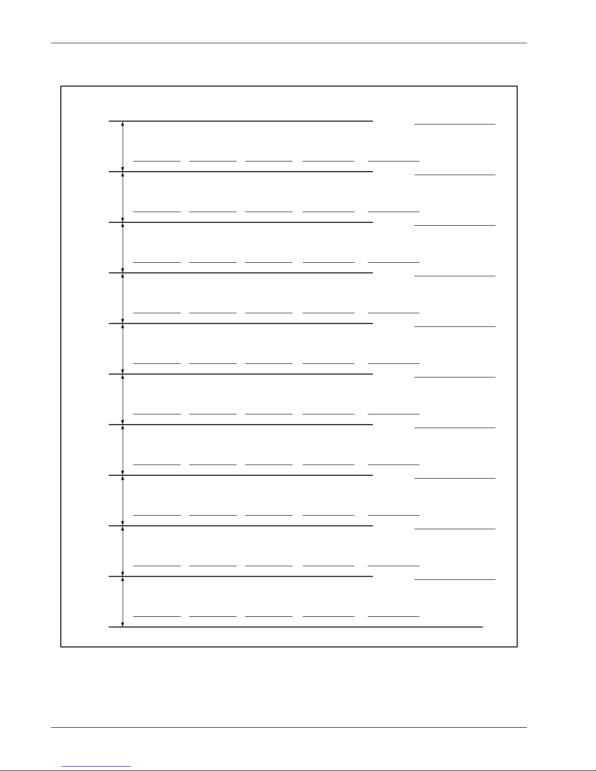
Lake Shore Model 340 Temperature Controller User’s Manual
Zone Setting WorkSheet
Zone 10
Zone 09
Zone 08
Zone 07
Zone 06
Zone 05
Setpoint:
Manual OutputGain (P) Reset (I) Rate (D)
Heater Range
Setpoint:
Manual OutputGain (P)Reset (I) Rate (D)
Heater Range
Setpoint:
Manual OutputGain (P) Reset (I) Rate (D)
Heater Range
Setpoint:
Manual OutputGain (P) Reset (I) Rate (D)
Heater Range
Setpoint:
Manual OutputGain (P) Reset (I) Rate (D)
Heater Range
Setpoint:
Manual OutputGain (P) Reset (I) Rate (D)
Heater Range
K
K
K
K
K
K
Zone 04
Manual OutputGain (P) Reset (I) Rate (D)
Zone 03
Manual OutputGain (P) Reset (I) Rate (D)
Zone 02
Manual OutputGain (P) Reset (I) Rate (D)
Zone 01
Manual OutputGain (P) Reset (I) Rate (D)
Setpoint:
Heater Range
Setpoint:
Heater Range
Setpoint:
Heater Range
Setpoint:
Heater Range
0 K
340-6-1.eps
K
K
K
K
0 K
Figure 6-1. Record of Zone Settings
6-6 Temperature Control Operation
Page 71

Lake Shore Model 340 Temperature Controller User’s Manual
6.9 USING OPEN LOOP CONTROL
Directly setting control output is called open loop control because there is no feedback from a load sensor to
close the control loop. Load temperature, setpoint, and control parameters are ignored. Use open loop control
for experiments requiring constant control output regardless of load temperature, for initial cooling system
tuning, or for when a computer calculates the control equation and sends output information to the instrument.
To use open loop control, set control mode to open (refer to Paragraph 6.5).
When using Control Loop 1 and the heater output, select an appropriate heater range. The manual output
parameter sets the control output as percent of full scale current or power on the selected heater range.
Manual Output setting range is -100% to +100% with a resolution of 0.01%. Change settings from the front
panel or with a computer interface. Negative values are not recommended when using the heater.
When using control Loop 2 and Analog Output 2, manual output parameter sets control output in percent of
the ±10 V range. Manual Output setting range is ±100% with a resolution of 0.01%. Negative values are not
recommended unless the output drives a device operating as a heating and cooling source. In most cases,
configure Analog Output 2 as unipolar when using it for control output.
To enter a manual output value, press Loop 1 or Loop 2 to display control parameters for that loop in the
lower portion of the display. Press Manual Output to highlight the MOut setting field. Enter a value with the
number keys and press Enter to save the change or Escape to return to the previous value. Default is 0.
6.10 SETTING A SETPOINT AND SETPOINT UNITS
The control setpoint is the desired load temperature expressed in temperature or sensor units. Use sensor
units if no temperature response curve is selected for the sensor input used as the control channel.
The control setpoint has its own units parameter. When the user selects sensor units as the setpoint units the
instrument calculates the control equation in sensor units. It calculates the control equation in temperature
with setpoint units set to kelvin or Celsius. The setpoint displays in the selected units. Adjust the P control
parameter when changing setpoint units from temperature to sensor. Control channel readings can display in
any units. Display units need not match setpoint units.
When changing setpoint units while the control loop is active, the Model 340 converts the control setpoint to
the new control units for minimal disruption in control output.
To select setpoint units, press Control Setup to display the CONTROL SETUP screen with the control loop
indicator highlighted in the upper left hand corner. Use the s or t key to select Loop 1 or 2. Press Enter or
Next Setting to display control setup parameters for that loop. Press Next Setting until the Setp Unit field
highlights. Use the s or t key to select units. Press Enter or Next Setting to continue with more settings, or
press Save Screen to store changes in the Model 340. Default is Temp K.
Setpoint resolution depends on sensor type and setpoint units. With setpoint expressed in temperature,
setpoint resolution is 0.001 degree for setpoints below 1000, and 0.0001 for setpoints below 10. In sensor
units, the setpoint resolution matches the display resolution for the sensor input type given in the
specifications (Table 1-1). If auto ranging sensor, enter a units multiplier of Ω or kΩ after the setpoint.
The instrument allows a large setpoint range to accommodate a variety of sensors and units. With setpoint
expressed in sensor units, setpoint range is unlimited. The user must determine suitability of a setpoint value.
In temperature units, two safety features limit the setpoint value to help prevent load damage load. The first
limit is the part of the temperature response curve that shows maximum safe temperature in kelvin for the
sensor package. It can be verified by using the Curve Entry key (Paragraph 8.1). The user may enter a
second global limit (Paragraph 6.13.1). Set it to the maximum safe temperature in kelvin for the entire system.
The setpoint is limited to a value less than or equal to the lower of the two safety limits.
After selecting setpoint units and limits, enter the setpoint value. Setpoint has a direct setting key because it
changes often. The setpoint value remains on the display any time control parameters for its control loop
display. If the setpoint value changes from the number entered when Enter is pressed, it is likely the setpoint
exceeds one of the above limits is inappropriate for the sensor type.
To enter a setpoint value, press Loop 1 or Loop 2 to display control parameters for that loop in the lower
portion of the display. Press Setpoint to highlight the setpoint setting field. Enter a value with the number
keys and press Enter to save the change or Escape to return to the previous value. Select a scale factor of
n, u, m, k, M, or G. Blank indicates a scale factor of x1. The default is 0.
Temperature Control Operation 6-7
Page 72

Lake Shore Model 340 Temperature Controller User’s Manual
6.11 SETPOINT RAMPING
The Model 340 generates a smooth setpoint ramp when the setpoint units are expressed in temperature. The
user can set a ramp rate in degrees per minute with a range of 0 to 100 and a resolution of 0.1. Once the
ramp feature is turned on, its action is initiated by a setpoint change. When a new setpoint is entered, the
instrument changes the setpoint temperature from the old value to the new value at the ramp rate. A positive
ramp rate is always entered and it is used by the instrument for ramps up and down in temperature.
The ramping feature is useful by itself but it is even more powerful when used with other features. Setpoint
ramps are often used with zone control mode. As temperature is ramped through different temperature zones,
control parameters are automatically selected for best control. Ramps are initiated and status read back using
a computer interface. During computer controlled experiments, the instrument generates the setpoint ramp
while the computer is busy taking necessary data. AutoTune does not function during a setpoint ramp
because the ramp rate disguises the reaction of the cooling system and no valid tuning data can be taken.
To turn on the ramp feature and set a ramp rate, press the Ramp key. The RAMP SETUP screen is displayed
with the control loop indicator highlighted in the top left hand corner. Use the s or t key to select Loop 1 or
2. Press the Enter or Next Setting key. The ramp setup information for that loop appears on the screen.
Press the Next Setting key until the Ramp field is highlighted. Use the s or t key to turn the ramp feature
On. Press the Next Setting key to highlight the ramp rate field. Use the number keys to enter a ramp rate
value and press the Save Screen key to save the changes in the Model 340. The default setting is Off, 0.1.
To stop a ramp in progress, press the Ramp key. The RAMP SETUP screen is displayed with the control loop
indicator highlighted in the top left hand corner. Use the s or t key to select Loop 1 or 2. Press the Enter or
Next Setting key. The ramp setup information for that loop appears on the screen. Press the Next Setting
key until the Ramp field is highlighted. Use the s or t key to turn the ramp feature OFF. Press the Save
Screen key to stop the ramp. Another method to stop the ramp is to press the Setpoint key then immediately
press the Enter key.
6.12 CONTROL OUTPUT
The output from the PID control equation in Loop 1 is directed to the heater output. The control output from
Loop 2 can only be directed to Analog Output 2. This section discusses using the heater output and an
Analog Output as a control output.
6.12.1 Heater Output Parameter Settings and Heater Range
Some difficulties may be encountered when configuring the heater output for the first time. It may be difficult
to judge the amount of heater power needed to control a cooling system before it tested. Another problem is
that the heater output is a current source and not a “power” source. The Model 340 itself adds confusion with
the number of available heater ranges.
There are three things that determine the full scale power of a given heater setup: heater resistance,
maximum current parameter, and the heater range parameter. Some typical heater output powers are given
in Table 6-2 to illustrate how these variables affect heater power.
The resistive heater is not included with the instrument. The cooling system determines the physical size,
location, and resistance of the heater (refer to Paragraph 2.4). A heater must be chosen that can dissipate the
full scale power available on the highest heater range that may be used. It is recommended to use a heater
with resistance between 10 Ω and 100 Ω. The nominal resistance of the heater should be entered into the
instrument so the display shows heater parameters properly in power units. An incorrect setting of heater
resistance does not change the operation of the heater output.
To enter a heater resistance, press the Control Setup key and the CONTROL SETUP screen is displayed.
The control loop indicator is highlighted in the upper left hand corner. Use the s or t key to select Loop 1.
Press the Enter or Next Setting key. The control setup parameters for that loop appear on the screen. Press
the Next Setting key until the Htr Ω field is highlighted. Use the number keys to enter the resistance of the
heater in ohms. Press the Enter or Next Setting key to continue with more settings, or press the Save
Screen key to store the changes in the Model 340. The default setting is 25 Ω.
6-8 Temperature Control Operation
Page 73
Lake Shore Model 340 Temperature Controller User’s Manual
The maximum current parameter is included in the Model 340 to make it more compatible with existing
cooling systems. Even though this instrument is capable of sourcing two amps of heater current, there are
many control loads that will not tolerate that much current. Lower maximum current settings let the instrument
source less current without loosing heater ranges or resolution. Maximum current choices: 2 A, 1A, 0.5 A, and
0.25 A.
To select a maximum heater current, press the Control Setup key and the CONTROL SETUP screen is
displayed. Press the More key until the CONTROL LIMITS screen is displayed. The control loop indicator is
highlighted in the upper left hand corner. Use the s or t key to select Loop 1. Press the Enter or Next
Setting key. The control setup parameters for that loop appear on the screen. Press the Next Setting key
until the Max Htr I (maximum heater current) field is highlighted. Use the s or t key to select from the list of
currents. Press the Enter key or next setting key to continue with more settings or press the Save Screen key
to store the changes in the Model 340. The default setting is 1 A.
The Model 340 heater output
has five ranges. Each range
(below the highest range)
reduces the full scale heater
output power. The ranges are
spaced at approximate
decades in power. The heater
range setting is available from
the normal display so that it
can be changed easily during
an experiment. For example,
with the maximum current set
to 1 A and a heater resistance
of 25 Ω, the heater output
provides the full scale current
and power shown in Table 6-3.
The range is displayed as the
maximum power computed
with the maximum current
setting and user specified
resistance. If the power does
not change when you change
the range, the voltage
compliance is limiting the
maximum power. If ranges are
skipped, the heater range limit
is set.
To select a heater output
Resistance Range 2 A 1 A 0.5 A 0.25 A
Table 6-2. Full Scale Heater Power at Typical Resistance
Heater Heater Maximum Current
10 Ω
25 Ω
35 Ω
50 Ω
5
4
3
2
1
5
4
3
2
1
5
4
3
2
1
5
4
3
2
1
40 W
4 W
0.4 W
40 mW
4 mW
100 W *
10 W
1 W
100 mW
10 mW
71.4 W
14 W
1.4 W
140 mW
14 mW
†
50 W
20 W
2 W
200 mW
20 mW
†
10 W
1 W
100 mW
10 mW
1 mW
25 W
2.5 W
250 mW
25 mW
2.5 mW
35 W
3.5 W
350 mW
35 mW
3.5 W
50 W
5 W
500 mW
50 mW
5 mW
2.5 W
250 mW
25 mW
2.5 mW
250 µW
6.25 W
625 mW
62.5 mW
6.25 mW
625 µW
8.75 W
875 mW
87.5 mW
8.75 mW
875 µW
12.5 W
1.25 W
125 mW
12.5 mW
1.25 mW
* Maximum power available. † Power limited by voltage compliance.
625 mW
62.5 mW
6.25 mW
625 µW
62.5 µW
1.56 W
156 mW
15.6 mW
1.56 mW
156 µW
2.19 W
219 mW
21.9 mW
2.19 mW
219 µW
3.12 W
312 mW
31.2 mW
3.12 mW
312 µW
range, indicate Loop 1 by
pressing the Loop 1 key. The control parameters for that loop
appear in the lower portion of the display. Press the Heater Range key and the setting field for heater range
is highlighted. Use the s or t key to select a heater
Table 6-3. Example of Max. Current Settings
range. Press the Enter key to save the change or the
Escape key to return to the previous setting. The
default setting is Off.
NOTE: The control output for Loop 1 must be
enabled before the heater can be turned on.
Refer to Paragraph 6.2.
The Model 340 has an immediate key operation for
Range Current Power
5 1 A 25 W
4 316 mA 2.5 W
3 100 mA 250 mW
2 31.6 mA 25 mW
1 10 mA 2.5 mW
turning the heater off. The Heater Off key is in a
prominent place on the keypad for easy access and it remains active when the keypad is locked. To turn off
the heater output, press the Heater Off key.
Temperature Control Operation 6-9
Page 74

Lake Shore Model 340 Temperature Controller User’s Manual
6.12.2 Analog Output As Loop 2 Control Output
The only control output available for Loop 2 is Analog Output 2. When the analog output is used as a control
output it has the same voltage range and resolution as it does when used for any other purpose. Many of the
settings and limits on the control setup and control limit screens apply to the Analog Output when used as a
control output. Heater range is the most obvious exception.
The analog outputs are variable DC voltage sources that can vary from ±10 V. The resolution of the analog
output is 1.25 mV or 0.0125% of full scale. The output can source up to 100 mA of current providing a
maximum of 1 W of power. They can drive a resistive load of no less than 100 Ω. The output is short
protected so the instrument is not be harmed if the heater resistance is too small. It is not recommended
because the additional load on instrument power supplies will cause noise on internal circuits.
Paragraph 3.5.7 describes two ways to use an Analog Output as a control output. If the output is used directly
as a resistive heater driver, be sure the heater has a resistance of 100 Ω or more. The maximum power out is
1 W at 100 Ω. If the output is used to program an external power supply, the input resistance of the voltage
programming input on the supply must be 100 Ω or greater. Setup and operation are otherwise similar.
To select control output as a source for an Analog
ANALOG OUTPUTSOutput: 2
Output, press the Analog Outputs key. The analog
output indicator is highlighted in the upper left hand
corner. Use the s or t key to select analog output
2. Press the Enter or Next Setting key until the
Mode:
Bipolar:
Status:
LOOP
OFF
0/0%
Mode field is highlighted. Use the s or t key to
select LOOP. Press Enter or Next Setting to
continue with more settings or the Save Screen key to save the changes to the Model 340.
It is recommended to set the Analog Output to unipolar mode. Few applications can use bipolar control
output. A thermoelectric cooling element is one example of a control actuator that can utilize a bipolar control
output. The AutoTune feature will not operate with Loop 2 configured for Bipolar Control.
To set unipolar operation for an Analog Output, press the Analog Outputs key. The analog output indicator is
highlighted in the upper left hand corner. Use the s or t key to select analog output 2. Press the Enter or
Next Setting key until the Bipolar field is highlighted. Use the s or t key to select OFF. Press the Enter or
Next Setting key to continue with more settings or the Save Screen key to save the changes to the Model
340.
Once the Analog Output is setup, the control loop must be setup. Control channel, control mode, PID control
parameters, setpoint units, and setpoint are described in the heater output Paragraph 6.12.1. The AutoTune
feature will only work with one loop at a time. Heater range and other features noted in Table 1-1 are not
available. Control output limits, other than heater range limit, described in Paragraph 6.13, work with any
control output.
6-10 Temperature Control Operation
Page 75

Lake Shore Model 340 Temperature Controller User’s Manual
6.13 CONTROL OUTPUT LIMITS
Control limits were added to the Model 340 as added protection to prevent parameter settings that can
damage the cooling system.
6.13.1 Setpoint Limit
Setpoint temperature limit is a global limit for a control loop. Setpoint values above the limit are rejected and
the setpoint defaults to the limit value. The limit is entered in kelvin and works with setpoint units of kelvin or
Celsius. The limit does not work when sensor units are chosen for the setpoint.
The Model 340 turns off the control output if the temperature of the control sensor exceeds the global limit.
The global setpoint limit works along with the individual limits that can be entered in a temperature response
curve. The curve limits are only active when a sensor using that curve is chosen as a control sensor while the
global limit is active all the time. The lower of the two is used to limit the setpoint.
To change the setpoint temperature limit, press the Control Setup key. The control loop indicator is
highlighted in the upper left hand corner. Use the s or t key to select a control loop and press the Enter or
Next Setting key. The control setup parameters for that loop appears on the screen. Press the Next Setting
key until the setpoint field under the limits heading is highlighted. Use the number keys to enter the maximum
setpoint in kelvin. Press the Enter or Next Setting key to continue with more settings, or press the Save
Screen key to store the changes in the Model 340. The default setting is 475 K.
6.13.2 Control Output Slope Limit
Some experiments can not tolerate fast changes in control output. The slope limit feature keeps changes in
control output below a user specified rate of change. There is a different limit for rising and falling slope. The
rising slope limit is shown as +Slope, the falling slope limit is shown as -Slope. Both are set in percent of
output current per second. The setting range is 0 to 100 with a resolution of 0.1.
To change the output slope limit, press the Control Setup key. The control loop indicator is highlighted in the
upper left hand corner. Use the s or t key to select a control loop and press the Enter or Next Setting key.
The control setup parameters for that loop appear on the screen. Press the Next Setting key until the slope
field under the limits heading is highlighted. Use the number keys to enter the maximum slope in percent per
second. Press the Enter or Next Setting key to continue with more settings, or press the Save Screen key to
store the changes in the Model 340. The default setting is 0 (off).
6.13.3 Heater Range Limit
Accidental heater range settings are possible because the heater range can be set directly from the normal
display of the Model 340. A heater range limit feature is intended to prevent heater range settings that could
harm the control load. The heater range can be set to the user specified limit setting but not above. The range
limit is accessed through control setup operation so it can not be changed unintentionally. The range limit is
only available for the heater output on Loop 1. The full scale power of a given heater range depends on the
maximum current setting so the maximum current parameter should be set before the range limit.
To change the heater range limit, press the Control Setup key. The control loop indicator is highlighted in the
upper left hand corner. Use the s or t key to select a control Loop 1 and press the Enter or Next Setting
key. The control setup parameters for that loop appear on the screen. Press the Next Setting key until the
range field under the limits heading is highlighted. Use the s or t key to select a range limit. Press the Enter
or Next Setting key to continue with more settings, or press the Save Screen key to store the changes in the
Model 340. The default setting is the highest range.
Temperature Control Operation 6-11
Page 76

Lake Shore Model 340 Temperature Controller User’s Manual
This Page Intentionally Left Blank
6-12 Temperature Control Operation
Page 77
Lake Shore Model 340 Temperature Controller User’s Manual
CHAPTER 7
ANALOG OUTPUT, DIGITAL I/O,
ALARM, AND RELAY OPERATION
7.0 GENERAL
The Model 340 has several hardware features that enable it to interface with the experimental environment.
These hardware features defined the operation of the controller as related to temperature measurement and
control, but can also be controlled manually by the user from the front panel or over computer interface.
Analog outputs are described in Paragraph 7.1. Digital inputs and outputs (I/O) are described in Paragraph
7.2. Input alarms are described in Paragraph 7.3. Finally, high and low relays are described in Paragraph 7.4.
7.1 ANALOG OUTPUTS
The Model 340 has two analog outputs, Analog Output 1 and Analog Output 2. They are voltage sources that
can be used to output a voltage representation of sensor input reading. Analog Output 2 can also be used as
the control output for Loop 2 as described in Paragraph 7.1.3. The user can select the source of the analog
output data and scale the relationship of data reading to output voltage, independently for the two analog
outputs.
The analog outputs are variable DC voltage sources that can vary from ±10 V. The resolution of the analog
output is 1.25 mV or 0.0125% of full scale. The output can source up to 100 mA of current providing a
maximum of 1 W of power. They can drive a resistive load of no less than 100 Ω. The output is short
protected so the instrument is not harmed if the load resistance is too small. This is not recommended
because the additional load on the power supplies in the instrument causes noise on the internal circuits. The
analog output connector and pinouts are shown in Figure 10-5.
To set up an analog output, first
select an operating mode. Other
parameters depend on the mode
that is selected. A list of analog
output operating modes is shown
to the right.
To select an analog output mode, press the Analog Outputs key. The ANALOG OUTPUTS screen is
displayed. With the output number highlighted in the top left corner, use the s or t key to select an analog
output. Press the Next Setting key until the Mode field is highlighted. Use the s or t key to select the
desired mode. Press the Next Setting or Enter key to make changes to other parameters, or press the Save
Screen key to store the changes. The default setting is Off.
OFF
INPUT
LOOP
MANUAL
Output voltage is set to 0 volts.
Analog output voltage is tied to a sensor input.
Control Loop 2 Control output (Analog Output 2 only).
Manual setting of the analog output voltage.
The analog output is capable of setting a bipolar (positive or negative) voltage. When the bipolar parameter is
on, the analog output varies between ±10 V. Many inputs may be damaged by a negative voltage. Setting the
bipolar parameter to off prevents the analog output from setting a negative output voltage. Only voltages
between 0 and +10 V are set. The bipolar setting is used for all of the analog output modes.
To set the bipolar parameter, press the Analog Outputs key. The ANALOG OUTPUTS screen is displayed.
With the output number highlighted in the top left corner, use the s or t key to select an analog output.
Press the Next Setting key until the bipolar field is highlighted. Use the s or t key to select ON or OFF.
Press the Next Setting or Enter key to make changes to other parameters or press the Save Screen key to
store the changes. The default setting is Off.
Analog, Digital, Alarm & Relay Operation 7-1
Page 78

Lake Shore Model 340 Temperature Controller User’s Manual
7.1.1 Input Mode for Analog Output
When input mode is
chosen for an analog
output, there are several
other parameters to set.
The sensor input must
be chosen and the data
source from the input.
Sensor input setup
including operation of
the linear equation is
discussed in Paragraph
5.3.3.
Once the sensor input
Input
Source
Low Reading data value that corresponds to -10 V when bipolar, 0 V
High Reading data value that corresponds to +10 V. The value may be set
Sensor Input used for input reading data. The default setting is A.
Source of data from the input. The default is Temp K.
Temp K Kelvin temperature reading from an input.
Temp C Celsius temperature reading from an input.
Sensor Sensor units reading from an input.
Linear Linear equation data from an input.
when unipolar. The value may be set as a six digit floating point
number. The default setting is 0.
as a six digit floating point number. The default setting is 1000.
data is directed to an analog output, there are two other parameters that must be set. The low and high
parameters define the 6-digit sensor input reading values that comprise the bottom and top of the analog
output voltage range. The scale factor can be selected as n, u, m, k, M, or G. Blank indicates a scale factory
of x1. These parameters are included so the user can control the range and sensitivity of the output. The
example below demonstrates how the high and low parameters work.
To configure an analog output, select the Mode and Bipolar setting, then continue with the other parameters
listed above. Highlight the parameter field and select the appropriate setting values. Press the Save Screen
key when finished to save the changes. The Value % field that appears is not a settable parameter in this
mode. It reports the analog output status in percent of full scale.
7.1.2 Example of Low and High Parameter Setting
With the analog output set
to linear mode, the
temperature input data
and voltage output data
Low High
Input A Temperature (K) 0 500 1000
|---------|---------|---------|---------|---------|---------|
Unipolar Output (V) 0 +5 +10
are related as shown:
The first figure results in a
wide temperature range
but sensitivity is poor. The
resulting sensitivity is
0.01 V/K or 10 mV/K.
Low High
Input A Temperature (K) 50 75 100
|---------|---------|---------|---------|---------|---------|
Unipolar Output (V) 0 +5 +10
If the application does not require a wide temperature range, the user can change the value of the low and
high parameters to improve sensitivity. This setup has a narrow range with much improved sensitivity of
0.2 V/K or 200 mV/K. Please note that in any application, the resolution of the analog output voltage is
always 1.25 mV as specified.
The second figure shows how sensitivity improves when working at liquid nitrogen temperature (77 K).
7.1.3 Loop 2 Mode for Analog Output 2
Discussion about using Analog Output 2 as the control output for Loop 2 is contained in the control operation
chapter. Loop 2 must be chosen as the mode for analog output 2 and the bipolar setting should match the
capability of the control system. It is recommended to set the Analog Output to unipolar mode. Few
applications can use bipolar control output. A thermo-electric cooling element is one example of a control
actuator that can utilize a bipolar control output.
7-2 Analog, Digital, Alarm & Relay Operation
Page 79
Lake Shore Model 340 Temperature Controller User’s Manual
7.1.4 Manual Mode Operation of the Analog Outputs
During manual operation, the user can set the voltage of an analog output giving them a controlled voltage
source. In manual mode, all analog output parameters are ignored except the bipolar setting and the users
output setting value.
The setting value is given in percent of full scale. With bipolar on, a setting value of -100 % causes an output
voltage of –10 V, and a setting value of +100 % causes an output voltage of +10 V. With bipolar off (unipolar)
a setting value of 0 % causes an output voltage of 0 V, and a setting value of +100 % causes an output
voltage of +10 V. Negative setting values cause an output voltage of 0 V if bipolar is off.
The resolution of the analog output hardware is 1.25 mV or 0.0125% of full scale. Setting resolution of the
output value is 0.01 %.
To set an analog output voltage, press the Analog Outputs key and set the mode to manual and set bipolar
setting as described in Paragraph 7.1. Press the Next Setting key until the value field is highlighted. Use the
number keys to enter the desired output, then press the Enter key. Press the Save Screen key to store the
changes. The default value is 0%.
7.2 DIGITAL INPUTS AND OUTPUTS (I/O)
The Model 340 has six digital inputs and five digital outputs. The digital inputs and outputs can be used to
monitor instrument status in a pre-programmed mode of operation or they can also be used in manual mode
to control and monitor external events. The connector pinout and hardware information about the digital
signals is provided in Paragraph 3.7. The digital signal lines are protected against short circuit and over
voltage but it is not recommended to expose the terminals to ESD or voltages higher than +5 V or lower than
ground provided on the Digital I/O connector.
7.2.1 Digital Output Modes
Model 340 digital outputs have
four modes of operation.
To select a digital output mode,
press the Options key. The
DIGITAL I/O screen appears
OFF
ALARMS
MANUAL
SCANNER
All digital outputs set to zero.
Used to indicate the alarm status of the sensor inputs.
Set by user from the front panel or computer interface.
Used with an external scanner (refer to Paragraph 5.4).
with the output mode
highlighted. Use the s or t key to select the desired mode. Press the Enter or Next Setting key to advance
to other settings, or press the Save Screen key to store changes. The default setting is Off.
7.2.2 Digital Outputs in Alarm Mode
In alarm mode, the digital outputs report the alarm status of the sensor input alarms. The digital output is low,
logic 0, to indicate no alarm condition and high, logic 1, to indicate an alarm condition exists. Alarms for a
given sensor input must be turned on for this feature to operate. The sensor input alarms are mapped to the
digital output signals as follows:
Input Alarm:
Digital Output Number:
Digital I/O Connector Pin:
* “Any Other” indicates that an alarm is active on any one of the installed optional inputs.
Any Other * B High B Low A High A Low
DO5 DO4 DO3 DO2 DO1
5 4 3 2 1
7.2.3 Digital Outputs in Scanner Mode
Digital outputs can be used to report the scan channel when an external scanner is being used. The digital
outputs must be put in scanner mode as described in Paragraph 7.2.1. External scanner operation is
described in Paragraph 5.4.
Analog, Digital, Alarm & Relay Operation 7-3
Page 80

Lake Shore Model 340 Temperature Controller User’s Manual
7.2.4 Digital Outputs in Manual Mode
In manual mode, the digital outputs are controlled directly by the user. The digital output signals can be set to
any combination of high (logic 1) or low (logic 0). Digital output can only be set using the 0 and 1 keys. For
example: a setting of 00011 causes digital outputs 1 and 2 to be high (logic 1) and digital outputs 3, 4, and 5
to be low (logic 0).
To manually set a digital output, set the digital output mode to manual as described in Paragraph 7.2.1. Press
the Options key and the Digital I/O screen appears. Press the Next Setting key until the Reading line is
highlighted. Use the number keys, 0 and 1, to enter a setting that corresponds to the digital output numbers
shown below the setting on the display. Press the Save Screen key to store the changes. The default value is
00000.
7.2.5 Digital Input Modes
The digital input signals are always read by the Model 340. Their status is always available from the front
panel or over computer interface. The only defined application of the digital inputs is during external scanner
operation (refer to Paragraph 5.4). If external scanner operation is not being used, the inputs are considered
to be in manual mode.
7.3 INPUT ALARMS
Each input of the Model 340 has a high and low alarm setting. Input reading data in temperature units, sensor
units, or from linear equation can be compared to the alarm values. If a reading is higher than the high alarm
setting the high alarm is active for the input. If a reading is lower than the low alarm setting the low alarm is
active for the input. The alarm feature can be enabled or disabled for each individual input.
Active alarms are indicated on the display with an annunciator. The Alarm annunciator indicates that there is
an input alarm enabled. An Alarming annunciator indicates that an enabled alarm is active. An audible
beeper can also sound to indicate an alarm is active. The audible beeper can be turned off for all alarms. One
or more sets of high and low alarms can be directed to the high and low alarm relays. Parameters on the
RELAY & BEEPER SETUP screen must be changed for the alarm relays and beeper to be active, as
described in Paragraph 7.4.
The alarms can operate in latching or non-latching mode. In non-latching mode, an active alarm becomes
inactive when the alarm condition is corrected. This mode is often used in control applications where an alarm
event is triggered inside the normal operating range of the input sensor. In latching mode an active alarm is
held active even after the alarm condition is corrected. This mode is most often used as a safety feature to
discontinue an external activity if the input sensor is outside of a safe operating range. The Alarm Reset key
is used to reset a latched alarm.
7.3.1 Enabling an Input Alarm
To enable an input alarm, press the Alarm Setup key. The ALARM SETTINGS screen appears with the input
letter in the top left hand corner. Use the s or t key to select an input. Press the Enter or Next Setting key
to show the alarm parameters for that input. Press the Next Setting key until the Enable field is highlighted.
Use the s or t key to turn the alarm on or off for that input. Use the Next Setting key to make more
changes, or press the Save Screen key to store the changes. The default setting is Enable Off.
7-4 Analog, Digital, Alarm & Relay Operation
Page 81
Lake Shore Model 340 Temperature Controller User’s Manual
7.3.2 Selecting an Input Alarm Source
Once an input is selected, a data
source from that input is set. The
following selections are available:
To select an input alarm data
source, press the Alarm Setup key.
TEMP K
TEMP C
SENSOR
LINEAR
Temperature in Kelvin.
Temperature in Celsius.
Raw sensor units as read from the input sensor.
Linear equation output, refer to Paragraph 5.3.3.
The ALARM SETTINGS screen
appears with the input letter in the top left hand corner. Use the s or t key to select an input. Press the
Enter or Next Setting key to show the alarm parameters for that input. Press the Next Setting key until the
source field is highlighted. Use the s or t key to select a source from that input. Use the Next Setting key to
make more changes or press the Save Screen key to store the changes. The default setting is Temp K.
7.3.3 Input Alarm High and Low Settings
High alarm and low alarm setting values for an input alarm are set with a 6-digit value and an additional scale
factor. The scale factor can be selected as n, u, m, k, M, and G. Blank indicates a scale factory of x1. If the
source is changed, the settings return to their default values. The instrument does not restrict the range or
resolution of the alarm setting.
To select an input alarm high or low setting, press the Alarm Setup key. The ALARM SETTINGS screen
appears with the input letter in the top left hand corner. Use the s or t key to select an input. Press the
Enter or Next Setting key to show the alarm parameters for that input. Press the Next Setting key until the
High or Low setting field is highlighted. Use the number keys to enter a value for the setting and press the
Enter key. Press the Enter key. Use the s or t key to select a scale factor: n, µ, m, k, M, and G. Blank
indicates a scale factory of x1. Press the Next Setting key to make more changes, or press the Save Screen
key to store the changes. The default values are Low = 0.0 and High = 1000.
7.3.4 Input Alarm Latching
To enable an alarm latching, press the Alarm Setup key. The ALARM SETTINGS screen appears with the
input letter in the top left hand corner. Use the s or t key to select an input. Press the Enter or Next Setting
key to show the alarm parameters for that input. Press the Next Setting key until the enable field is
highlighted. Use the s or t key to turn alarm latching on or off for that input. Use the Next Setting key to
make more changes or press the Save Screen key to store the changes. The default setting is Off.
7.3.5 Input Alarm Relay Setup
The two relays on the Model 340 can be used for high and low alarm outputs. One or more sets of high and
low input alarms can be directed to the high and low relays. To direct the alarms from an input to the relays,
set the relay parameter on the ALARM SETTINGS screen to On. Parameters on the RELAY & BEEPER
SETUP screen must also be changed, as described in Paragraph 7.4.
When the alarms directed to a relay are not active (status Off), the relay is in the normal position. If any one of
the alarms directed to a relay is active (status On), the relay switches to the opposite position. Relay
connections are shown in Figure 3-7.
To direct an alarm pair to the relays, press the Alarm Setup key. The ALARM SETTINGS screen appears
with the input letter in the top left hand corner. Use the s or t key to select an input. Press the Enter or Next
Setting key to show the alarm parameters for that input. Press the Next Setting key until the enable relay is
highlighted. Use the s or t key to turn the relay parameter on or off for that input. Use the Next Setting key
to make more changes or press the Save Screen key to store the changes. The default setting is Off.
Analog, Digital, Alarm & Relay Operation 7-5
Page 82

Lake Shore Model 340 Temperature Controller User’s Manual
7.3.6 Input Alarm Reset
The Alarm Reset key performs the immediate action of resetting all latched alarms. If any alarm is latched
active and the alarm condition has been corrected, pressing the Alarm Reset key deactivates the alarm. If
the alarm condition is not corrected, the alarm is not deactivated. Non-latching alarms deactivate when the
alarm condition is corrected without the Alarm Reset function.
7.3.7 Audible Beeper
The audible alarm beeper can be turned on or off for the entire instrument. To turn on or off the audible alarm
beeper, press the Options key and then press the More key and the RELAYS & BEEPER SETUP screen
appears. Press the Next Setting key until the beeper field highlights. Use the s or t key to turn the beeper
on or off and press the Save Screen key to store the change. The default setting is On.
7.4 HIGH AND LOW RELAYS
The Model 340 has one high and one low
relay. See Figure 3-7. They are most
commonly associated with the alarm feature
discussed in Paragraph 7.3. The relays can
OFF
MANUAL
ALARMS
Relay is set to Off
Relay manual control (Paragraph 7.4.2)
Relay triggered by alarm (Paragraph 7.3.5)
also be put in manual mode and controlled
directly by the user from the front panel or over computer interface. Relay parameters are shown on the
Relays and Beeper Setup screen, which is accessed by pressing the Options key, then pressing the More
key. The relay and beeper Status shown on the right side of the screen is for monitoring only and cannot be
changed by the user.
7.4.1 Selecting a Relay Mode
To select a relay mode, press the Options key and then press the More key and the RELAYS & BEEPER
SETUP screen appears. Press the Next Setting key until the appropriate relay mode field is highlighted. Use
the s or t key to select a mode for that relay. Use the Next Setting or Enter key to make more changes or
press the Save Screen key to store the changes. The default setting is Off.
7.4.2 Manually Setting a Relay
To manually control a relay it must be in the manual mode, as described in Paragraph 7.4.1. A relay setting of
“Off” puts the relay in its normal state, while “On” puts the relay in the opposite state.
To change a relay setting, press the Options key and then press the More key and the RELAYS & BEEPER
SETUP screen appears. Press the Next Setting key until the appropriate relay setting field is highlighted. Use
the s or t key to select on or off for that relay. Use the Next Setting or Enter key to make more changes or
press the Save Screen key to store the changes. The default setting is Off.
7-6 Analog, Digital, Alarm & Relay Operation
Page 83

Lake Shore Model 340 Temperature Controller User’s Manual
CHAPTER 8
INSTRUMENT PROGRAMMING
8.0 GENERAL
The Model 340 has a powerful processor, user interface, and special programming features. Internal
programming is not intended to replace computer interface operation, and in most cases the two complement
each other. Programming features include entering a temperature response curve, saving and restoring
instrument parameters, and internal programming that allows the instrument to run temperature profiles.
This chapter covers front panel curve entry in Paragraph 8.1, SoftCal™ in Paragraph 8.2), internal
programming in Paragraph 8.3, and data card operations in Paragraph 8.4.
8.1 CURVE ENTRY FROM THE FRONT PANEL
Enter a temperature response curve into the Model 340 in several ways: Field install a CalCurve with a Data
Card or order it factory-installed; enter a user-generated curve from the front panel; create a SoftCal curve
with the SoftCal feature (Paragraph 8.2); or load a curve with a computer interface (refer to Chapter 9).
8.1.1 Curve Numbers and Storage
The Model 340 has 20 standard curve locations; numbered 1 thru 20. At present, only curve locations 1 thru
10 are occupied by curves; the others are reserved for future updates. If a standard curve location is in use,
the curve can be viewed using the edit operation. Standard curves can not be changed by the user, and
reserved locations are not available for user curves.
The Model 340 has 40 user curve locations numbered 21 thru 60. Each location can hold from 2 to 200 data
pairs (breakpoints) including a value in sensor units and a corresponding value in Kelvin. Using fewer than
200 breakpoints will not increase the number of available curve locations. SoftCal generated curves are
stored in user curve locations.
No specific curve endpoints are required. The instrument will show an error message on the display if the
sensor input is outside the range of the breakpoints.
Each curve has a set of parameters that are used for identification and to allow the instrument to use the
curve effectively. The parameters must be set correctly before a curve can be used for temperature
conversion or temperature control.
Please note that if instrument power is lost when new curves are being stored or erased (Save Screen has
been pressed), all user curves may be lost.
8.1.2 Front Panel Curve Entry Operations
There are three operations associated with front panel curve entry: Edit curve, Copy curve copy, Erase curve;
as detailed below.
Edit curve
Edit allows the user to see any curve and enter or edit a curve at any user
curve location. Standard curves cannot be changed (Paragraph 8.1.3).
Copy allows the user to copy a curve from any location to any user curve
Copy curve
location. Curves cannot be copied into standard curve locations
(Paragraph 8.1.4).
Erase curve
Erase allows the user to delete a curve from any user curve location.
Standard curves cannot be erased (Paragraph 8.1.5).
To begin a curve operation, press the Curve Entry key and the above selections appear. Press the Next
Setting key until the desired operation is highlighted and press the Enter key. A curve screen appears with
the curve number highlighted. Change to the desired curve number with the s or t key, then press the Enter
key to begin the desired curve operation.
Instrument Programming 8-1
Page 84
Lake Shore Model 340 Temperature Controller User’s Manual
8.1.3 Front Panel Curve Edit
The Edit curve operation can be used to enter a new curve or edit an existing user curve. Entering the
identification parameters associated with the curve is as important as entering the breakpoints. Only user
curves (numbers 21 to 60) can be changed. Standard curves can only be viewed with the edit operation.
Identify curves with names of up to 15 characters. The curve name cannot be changed
Name:
during front panel curve entry. To change curve names, enter them over computer interface.
The default curve name is User xx, where xx is the curve number.
Identify specific sensors with serial numbers of up to 10 characters. The serial number field
SN:
accepts both numbers and letters, but the instrument front panel enters only numbers. To
enter both numbers and letters enter curves over computer interface. The default is blank.
A setpoint temperature limit can be included with every curve. If the control sensor is an
Limit
input using a curve and operating in temperature units, then the setpoint cannot exceed the
limit entered with the curve. The default is 375 K.
The instrument must know the data format of the curve breakpoints. Different sensor types
use different data formats. The standard sensor inputs require one of the formats below. The
range and resolution specified are not always available at the same time. Practical range
Format:
and resolution depend on the sensor type.
Sensor Units Sensor Units
Format Description Full Scale Range Maximum Resolution
V/K Volts vs. Kelvin 10 (V) 0.00001 (V)
Ω/K Resistance vs. Kelvin 10 k (Ω) 0.00001 (Ω)
log R/ K log Resistance vs. Kelvin 4 (log R) 0.00001 (log R)
log R / log K log Resistance vs. log Kelvin 4 (log R) 0.00001 (log R)
mV/K mV vs. Kelvin ±100 (mV) 0.00001 (mV)
Enter an appropriate temperature for proper temperature control. A positive coefficient
indicates the sensor signal increases with increasing temperature. A negative coefficient
Coeff:
indicates the sensor signal decreases with increasing temperature. The instrument derives
the temperature coefficient from the first two breakpoints. If it is set improperly, check the
first two breakpoints.
Table 8-1. Recommended Curve Parameters
Type
Lake Shore
Model No.
Units Format Limit (K) Coefficient
Recommended
Sensor Resolution
Silicon Diode DT-470 Volts V/K 475 Negative 0.00001 (V)
GaAlAs Diode TG-120 Volts V/K 325 Negative 0.00001 (V)
Platinum 100 PT-100 Ohms Ohm/K 800 Positive 0.001 (Ω)
Platinum 1000 PT-100 Ohms Ohm/K 800 Positive 0.01 (Ω)
Rhodium-Iron RF-100 Ohms Ohm/K 325 Positive 0.001 (Ω)
Carbon-Glass CGR-1-1000 Ohms logR/K 325 Negative 0.00001(logR)
Cernox CX-1030 Ohms logR/K 325 Negative 0.00001(logR)
Ruthenium Oxide - Ohms logR/K 325 Negative 0.00001(logR)
Germanium GR-200A-100 Ohms logR/K 325 Negative 0.00001(logR)
Once curve identification parameters are entered, it is time to enter curve breakpoints. A breakpoint is the
representation of the sensor calibration that is stored in the instrument. Each breakpoint consists of one value
in sensor units and one temperature value in kelvin. From 2 to 200 breakpoints can be entered as a curve. No
special endpoints are required. Sensor units are defined by the format setting in Table 8-1.
Breakpoint setting resolution is six digits in temperature. Most temperature values are entered with 0.001
resolution. Temperature values of 1000 K and greater can be entered to 0.01 resolution. Temperature values
below 10 K can be entered with 0.0001 resolution. Temperature range for curve entry is 1500 K.
8-2 Instrument Programming
Page 85

Lake Shore Model 340 Temperature Controller User’s Manual
Setting resolution is also six digits in sensor units. The curve format parameter defines the range and
resolution in sensor units as shown in Table 8-1. The sensor type determines the practical setting resolution.
Table 8-1 lists recommended sensor units resolutions. For most sensors, additional resolution is ignored.
The breakpoints should be entered with the sensor units value increasing as point number increases. There
should not be any breakpoint locations left blank in the middle of a curve. The search routine in the Model 340
interprets a blank breakpoint as the end of the curve.
NOTE: If the curve you wish to enter has similar parameters to an existing curve, first copy the similar curve
(as described in Paragraph 8.1.5) to a new location, then edit the curve to the desired parameters.
To enter a curve, press the Curve Entry key. Press
the Next Setting key until Edit curve is selected,
then press the Enter key. Use the s or t key to
select the desired curve number to edit, then press
the Enter key.
You may now enter the serial number (SN), Limit,
Name:
Limit:
Format:
Coeff:
Edit Curve: #23
DT-470
SN:
D20496
499.900
V/K
Neg.
(I)I n s e r t
Sensor
1:
0.09062
2:
0.10191
3:
0.11356
4:
0.12547
5:
0.13759
(D )D e le t e
Temp(K)
475.000
470.000
465.000
460.000
455.000
Format, and Sensor/Temp (K) breakpoint pairs. Use the Previous Setting and Next Setting keys to move
from one edit field to the next. Use the I and D keys to Insert or Delete lines from the breakpoint field. When
the edit is complete, press the Save Screen key. The Saving user curves... message appears for a few
seconds. If you do not wish to save the new curve, press the Cancel Screen key.
8.1.4 Front Panel Curve Copy
Curves can be copied from one location inside the Model 340 to another. This is a good way to make small
changes to an existing curve. Curve copy may also be necessary if the user needs the same curve with two
different temperature limits or needs to extend the range of a standard curve. The curve that is copied is
always preserved.
NOTE: Copying an internal curve from one location to another is not the same as copying (or
downloading) a curve from a data card to the Model 340. The data card curve downloading
procedure is provided in Paragraph 8.4.
To copy a curve, press the Curve Entry key. Press
the Next Setting key until Copy curve is selected,
then press the Enter key.
Change to the desired curve number with the s or
t key, then press the Enter key. The cursor jumps
Name:
Limit:
Format:
Coeff:
Copy Curve: #1 To: #21
SN:
DT-470
Sta ndard
499.900
V/K
Neg.
1:
2:
3:
4:
5:
Sensor
0.09062
0.10191
0.11356
0.12547
0.13759
Temp(K)
475.000
470.000
465.000
460.000
455.000
to the To: selection. Again, use the s or t key to
select the user curve number (21 to 60) the curve will be copied to. (Empty user curves have zeros for data.)
NOTE: The copy routine allows you to overwrite an existing user curve. Please ensure the curve number
you are writing to is correct before proceeding with curve copy.
Once the curve number to copy to has been selected, press the Enter key. The following message is
displayed: Press SAVE SCREEN to copy, CANCEL SCREEN to abort. If you press the Save Screen key,
the Saving user curves... message appears for a few seconds, then the display returns to the CURVE
ENTRY menu. If you press the Cancel Screen key, the curve is not copied and you are returned to the
CURVE ENTRY menu.
8.1.5 Front Panel Curve Erase
When curves are no longer needed, they can be edited over or erased. Curves erase sets all identification
parameters to default and blanks all breakpoint values.
To erase a curve, press the Curve Entry key. Press the Next Setting key until Erase curve is selected, then
press the Enter key. Change to the desired curve number with the s or t key, then press the Enter key. The
following message is displayed: Press SAVE SCREEN to erase, CANCEL SCREEN to abort. If you press
the Save Screen key, the Saving user curves... message appears for a few seconds, then the display
returns to the CURVE ENTRY menu. If you press the Cancel Screen key, the curve is not erased and you
return to the CURVE ENTRY menu.
Instrument Programming 8-3
Page 86

Lake Shore Model 340 Temperature Controller User’s Manual
8.2 SOFTCAL™
The Model 340 performs inexpensive sensor calibrations with a two algorithms called SoftCal. These
algorithms work with DT-400 Series Silicon Diode sensors and Platinum Sensors. They create a new
temperature response curve from the standard curve and known data points entered by the user. The new
curve loads into one of the 40 user curve locations (21 thru 60). These paragraphs describe the data points
needed from the user and the expected accuracy of the resulting curves.
Both DT-400 and Platinum SoftCal algorithms require an existing standard curve in the Model 340. When the
user enters the sensor type to calibrate, the correct standard curve is selected. When calibration is complete,
the user selects the new curve for an input; the Model 340 does not automatically choose the newly
generated curve for either input.
Enter calibration data points (normally measured at easily reached temperatures). Each algorithm operates
with one, two, or three calibration points. Accuracy increases with more points.
There are two ways to get SoftCal calibration data points: n The user record the response of an unknown
sensor at well controlled temperatures, or o The user buys a Lake Shore SoftCal calibrated sensor. There
are advantages to both methods.
n User: When the user can provide stable calibration temperatures with the sensor installed, SoftCal
calibration eliminates errors in the sensor measurement as well as the sensor. Thermal gradients,
instrument accuracy, and other measurement errors can be significant. Calibration can be no better than
user-supplied data.
o Purchased: Lake Shore sensors with SoftCal calibration include a set of calibration points in the
calibration report. Lake Shore generates SoftCal calibration points in a controlled calibration facility for best
accuracy. The user enters the calibration points into the Model 340 to generate a curve. If the user buys
the CalCurve service with the calibrated sensor, the factory generates the curve for later entry like any
other curve.
8.2.1 SoftCal and Silicon Diode Sensors
Lake Shore Silicon Diode Sensors incorporate remarkably uniform sensing elements that exhibit precise,
monotonic, and repeatable temperature response. For example, the Lake Shore DT-470 Series of silicon
diode sensors has a repeatable temperature response from 2 K to 475 K. These sensors closely follow the
Standard Curve 10 response and routinely interchange with one another. SoftCal is an inexpensive way to
improve the accuracy of an already predictable sensor.
NOTE: Standard Curve 10 is the name of the temperature response curve, not its location inside
the Model 340. Standard Curve 10 is stored in Curve Location #1 in the Model 340.
A unique characteristic of DT400 Series diodes is that their
temperature responses pass
through 28 K at almost exactly
SoftCal Point 1 SoftCal Point 2
Liquid Helium
Boiling Point
4.2 K
Liquid Nitrogen
Boiling Point
77.35 K
SoftCal Point 3
Room
Temperature Point
305 K
the same voltage. This improves
SoftCal algorithm operation by
providing an extra calibration
data point. It also explains why
SoftCal calibration specifications
are divided into two temperature
ranges, above and below 28 K.
0 25 50 75 100 125 150 17 5 20 0 22 5 25 0 27 5 30 0 325 350 kel vin
2 - 10 K 50 - 100 K 200 - 325 K
Acceptable Temperature Range for Silicon Diode SoftCal Inputs
Figure 8-1. SoftCal Temperature Ranges for Silicon Diode Sensors
See Figure 8-1.
Point 1: Calibration data point at or near the boiling point of helium, 4.2 K. Temperatures outside 2 K to 10 K
are not allowed. This data point improves between the calibration data point and 28K. Points 2 and 3 improve
temperatures above 28 K.
Point 2: Calibration data point at or near the boiling point of nitrogen (77.35 K). Temperatures outside 50 K to
100 K are not allowed. This data point improves accuracy between 28 K and 100 K. Points 2 and 3, together,
improve accuracy to room temperature and above.
Point 3: Calibration data point near room temperature (305 K). Temperatures outside the range of 200 K to
350 K are not allowed.
8-4 Instrument Programming
Page 87

Lake Shore Model 340 Temperature Controller User’s Manual
8.2.2 SoftCal Accuracy with Silicon Diode Sensors
SoftCal allows an abbreviated calibration, based on 1, 2, or 3 points, to generate a voltage-versustemperature curve over the useful range of a Lake Shore DT-400 Series silicon diode sensor.
A SoftCal calibration is only as good as the accuracy of the calibration points. The accuracies listed for
SoftCal assume ±0.05 K for 77.35 K (liquid nitrogen) and 305 K (room temperature) points, and ±0.01 K for
4.2 K (liquid helium). Users performing the SoftCal with silicon diodes and Lake Shore instruments should
note that liquefied nitrogen and ice point temperatures can vary as much as ±0.5 K. Use calibrated standard
sensors if possible. The boiling point of liquid helium, though accurate, is affected by atmospheric pressure.
Perform one-point SoftCal calibrations for applications under 30 K at liquid helium (4.2 K). Accuracy for the
DT-470-SD-13 diode is ±0.5 K from 2 K to <30 K with no accuracy change above 30 K.
Perform two-point SoftCal calibrations for applications above 30 K at liquid nitrogen (77.35 K) and room
temperature (305 K). Accuracy for the DT-470-SD-13 diode sensor is as follows:
±1.0 K from 2 K to <30 K (no change below 30 K)
±0.25 K from 30 K to <60 K ±0.25 K from 345 K to <375 K
±0.15 K from 60 K to <345 K ±1.0 K from 375 to 475 K
Perform three-point SoftCal calibrations at liquid helium (4.2 K), liquid nitrogen (77.35 K), and room
temperature (305 K). Accuracy for the DT-470-SD-13 diode sensor is as follows:
±0.5 K 2 K to <30
±0.25 K 30 K to <60 K ±0.25 K 345 K to <375 K
±0.15 K 60 K to <345 K ±1.0 K 375 to 475 K
8.2.3 SoftCal and Platinum Sensors
The platinum sensor is a well-accepted temperature standard because of its consistent and repeatable
temperature response above 30 K. SoftCal gives platinum sensors better accuracy than their nominal
matching to the DIN 43760 curve.
Use one, two, or three calibration data
points. If using one point, the algorithm
shifts the entire curve up or down to
meet the single point. If using two
SoftCal Point 1 SoftCal Point 2 SoftCal Point 3
Liquid Nitrogen
Boiling Point
77.35 K
Room
Temperature Point
305 K
High
Temperature Point
480 K
points, the algorithm has enough
information to tilt the curve, achieving
good accuracy between the data points.
The third point extends the improved
accuracy to span all three points.
Point 1: Calibration data point at or
0 50 100 150 200 250 30 0 35 0 kel vin
50 - 100 K 200 - 325 K 400 - 600 K
Acceptable Temperature Range for Platinum SoftCal Inputs
400 450 500 55 0 60 0 65 0
Figure 8-2. SoftCal Temperature Ranges for Platinum Sensors
near the boiling point of nitrogen (77.35
K). Temperatures outside 50 K to 100 K are not allowed.
Point 2: Calibration data point near room temperature (305 K). Temperatures outside 200 K to 350 K are not
allowed.
Point 3: Calibration data point at a higher temperature (480 K). Temperatures outside 400 K to 600 K are not
allowed.
8.2.4 SoftCal Accuracy with Platinum Sensors
The SoftCal procedure makes small adjustments to the DIN curve so that the resulting curve matches the
resistance-versus-temperature characteristic of the individual sensor more closely.
A SoftCal calibration is only as good as the accuracy of the calibration points. The accuracies listed for
SoftCal assume ±0.05 K for 77.35 (liquid nitrogen) K and 305 K (room temperature) points. If you are
performing the SoftCal yourself with Lake Shore instrumentation, be aware that liquefied nitrogen and ice
point temperatures can vary as much as ±0.5 K. Use a calibrated standard sensor if possible. One-point
SoftCal calibrations with platinum sensors have no specified accuracy.
Instrument Programming 8-5
Page 88

Lake Shore Model 340 Temperature Controller User’s Manual
Perform two-point SoftCal calibrations for applications above 70 K at liquid nitrogen (77.35 K) and room
temperature (305 K). Accuracy for the PT-102, PT-103, or PT-111 platinum sensor is as follows:
±250 mK from 70 K to 325 K ≈±500 mK from 325 K to ≈±1400 mK at 480 K
(DIN Class A or Class B tolerance)
Perform three-point SoftCal calibrations at liquid nitrogen (77.35 K), room temperature (305 K), and high
temperature (480 K). Accuracy for the PT-102, PT-103, or PT-111 platinum sensor is
325 K, and ±250 mK from 325 K to 480 K.
±250 mK from 70 K to
8.2.5 Creating a SoftCal Calibration Curve
Once the calibration data points have been
obtained, you may create a SoftCal calibration.
Press SoftCal.
Use the s or t key to select the Standard curve
that the SoftCal will be based on. Press the Enter
key. Use the numerical keypad to enter the location
Std. Curve:
User Curve:
SOFTCAL
1 D T -4 7 0
21 SN:
Point 1:
Point 2:
Point 3:
Temp.
4.2000
77.3500
305.000
Reading
1.62622
1.02032
0.50691
where the new user curve will be stored. Press the Enter key. Use the numerical keypad to enter from 1 to 10
digits for a sensor serial number. Press the Enter key. Enter the first temperature and corresponding sensor
reading. Press the Enter key. Repeat the process for the next two temperature points. When complete, press
the Save Screen key. You see a brief Generating Curve message, followed by a longer Saving user
curves... message. The SoftCal curve has now been generated. The new curve has the name SCAL XXY
where XX is DT for diodes and PT for platinum, and Y specifies how many points were used to generate the
curve. Once the curve is generated, you must remember to select the curve for the desired input. Refer to
Paragraph 5.2.
8.3 INTERNAL PROGRAMMING
Internal programming allows the user to enter a set of simple instructions, called a program, into the
instrument. Some instructions mimic front panel operations; like setpoint ramps and control parameter
changes. Other instructions are for timing and decision making. The instrument can run the instructions in an
internal program without operator interaction. Since program status can be monitored with a computer
interface, internal programs can be used during computer controlled experiments.
The internal program feature works with control Loop 1. There is enough memory in the Model 340 to hold
100 programming instructions. The instructions can be put in up to 10 different program locations. The
program locations are provided to help organize internal programming operations. As many as 100 and as
few as 2 or 3 instructions can be placed in a single program location. The total number of instructions in all
ten program locations must not exceed 100. An End instruction, described in the next paragraph, is included
in each program location but does not take one of the 100 memory locations.
The following paragraphs provide details about the programming instructions offered in the Model 340, then
gives an example of how to put the instructions together into a program. A second example illustrates how
programs in two or more program locations can be used together.
8.3.1 Program Instructions
The Model 340 has 13 programming instructions divided into three categories: output ramping, direct setting
operations, and flow control. The instructions are listed below with paragraph references.
Command Display Paragraph Command Display Paragraph
Output Ramping Flow Control
Ramp Setpoint Absolute Ramp SP Abs. 8.3.1.1 Wait Wait 8.3.1.8
Ramp Setpoint Relative Ramp SP Rel. 8.3.1.2 Settle Settle 8.3.1.9
Ramp Manual Output Absolute Ramp MOut Abs. 8.3.1.3 Repeat Repeat 8.3.1.10
Ramp Manual Output Relative Ramp MOut Rel. 8.3.1.4 End Repeat End Repeat 8.3.1.10
Direct Settings Call Call 8.3.1.11
Control Parameters Parameters 8.3.1.5 End End 8.3.1.12
Digital Output Digital Output 8.3.1.6 No Operation NOP 8.3.1.13
Relays Relays 8.3.1.7
8-6 Instrument Programming
Page 89

Lake Shore Model 340 Temperature Controller User’s Manual
8.3.1.1 Ramp Setpoint Absolute
Ramp the control setpoint from its present setting value to a new specified (absolute) setting value. The
setpoint units must be in temperature for this instruction to operate. The ramp can be done at a specified
ramp rate or in a specified length of time. This instruction is used with a closed loop temperature control
mode. If the instrument is configured for Zone control mode, the control parameters including heater range
are updated as the setpoint temperature changes through new zones. Setpoint ramps in an internal program
override the stand alone setpoint ramp parameter.
Setpoint: New Loop 1 control setpoint in temperature units.
Hours: Hours to ramp to new setpoint (0 to 23).
Minutes: Minutes to ramp to new setpoint (0 to 59).
Seconds: Seconds to ramp to new setpoint (0 to 59).
Rate: Ramp rate in kelvin per minute (K/m) from 0 to 100
Ramp SP Abs. >|Setpoint: 0.000K
| Hours: 0
| Minutes: 0
| Seconds: 0
| Rate: 0.0K/m
with 0.1 resolution.
NOTE: Ramp time or ramp rate can be set, but not both. If ramp time and rate are both zero,
then the ramp is a step change.
8.3.1.2 Ramp Setpoint Relative
Ramp the control setpoint a specified difference (relative) from its present setting value. The setpoint units
must be in temperature for this instruction to operate. The ramp can be done at a specified ramp rate or in a
specified length of time. This instruction is used with a closed loop temperature control mode. If the
instrument is configured for in Zone control mode, the control parameters including heater range are updated
as the setpoint temperature changes through new zones. Setpoint ramps in an internal program override the
stand alone setpoint ramp parameter.
Dev: Deviation in Loop 1 control setpoint, temperature units,
bipolar.
Hours: Hours to make setpoint deviation (0 to 23).
Minutes: Minutes to make setpoint deviation (0 to 59).
Seconds: Seconds to make setpoint deviation (0 to 59).
Ramp SP Rel. >| Dev.: 0.000K
| Hours : 0
|Minutes: 0
|Seconds: 0
| Rate : 0.0K/m
Rate: Ramp rate in kelvin per minute (K/m) from 0 to 100
with 0.1 resolution.
NOTE: Ramp time, ramp rate, and deviation are related. The instrument calculates a ramp rate based on
deviation and ramp time. If ramp time and rate are both zero, then the ramp is a step change.
8.3.1.3 Ramp Manual Output (MOut) Absolute
Ramp the manual output (MOut) from its present setting value to a new specified (absolute) setting value. The
setting is in percent of full scale output which is normal for the manual output parameter. The ramp can be
done at a specified ramp rate or in a specified length of time. This instruction is used with the open loop
temperature control mode.
Output: New Loop 1 control output in percent of full scale.
Hours: Hours taken to ramp to new output (0 to 23).
Minutes: Minutes to ramp to new output (0 to 59).
Seconds: Seconds to ramp to new output (0 to 59).
Rate: Ramp rate in percent per minute (%/m) from 0 to 100
Ramp MOut Abs. >| Output: 0.00%
| Hours: 0
|Minutes: 0
|Seconds: 0
| Rate: 0.00%/m
with 0.1 resolution.
NOTE: Ramp time or ramp rate can be set but not both. If ramp time and rate are both zero, then
the ramp is a step change.
Instrument Programming 8-7
Page 90

Lake Shore Model 340 Temperature Controller User’s Manual
8.3.1.4 Ramp Manual Output (MOut) Relative
Ramp the manual output (MOut) a specified difference (relative) from its present setting value. The setting is
in percent of full scale output which is normal for the manual output parameter. The ramp can be done at a
specified ramp rate or in a specified length of time. This instruction is used with the open loop temperature
control mode.
Dev: Deviation in Loop 1 control output set in percent of
full scale.
Hours: Hours to make output deviation (0 to 23).
Minutes: Minutes to make output deviation (0 to 59).
Seconds: Seconds to make output deviation (0 to 59).
Rate: Ramp rate in percent per minute (%/m) from 0 to
Ramp MOut Rel.>| Dev.: 0.00
| Hours: 0
|Minutes: 0
|Seconds: 0
| Rate: 0.00%/m
100 with 0.1 resolution.
NOTE: Ramp time, ramp rate, and deviation are related. The instrument calculates a ramp rate based on
deviation and ramp time. If ramp time and rate are both zero, then the ramp is a step change.
8.3.1.5 Control Parameters
During many experiments it may be necessary to change control parameters. This need is particularly great
when making large changes in temperature. Common control parameters can be set with this instruction. The
AutoTune control mode is not available during internal program operation. Setpoint units are not changeable,
the setpoint units parameter should be set to temperature before running an internal program.
Channel: Loop 1 control channel.
Mode: Loop 1 control mode.
P, I, D: Loop 1 control parameters. Set with zone feature
if zone control mode is selected above.
Htr. Range: Loop 1 heater output range. Set maximum
heater current before running an internal program.
Parameters >| Channel: A
| Mode: MANUAL PID
| P: 0.0
| I: 0.0
| D: 0
|Htr Range: OFF
8.3.1.6 Digital Output
A Model 340 internal program can interact with experimental parameters other than temperature. The digital
outputs can be used to control outside events while a program is running. Using digital outputs in programs is
not available if external scanner operation is enabled.
Settings: Refer to Paragraph 7.2.
Digital Output >|Setting: 00000
| 54321
8.3.1.7 Relays
A Model 340 internal program can interact with experimental parameters other than temperature. The high
and low relays can be used to control outside events while a program is running. Relays must be set to
Manual for operation.
Relays: High and low relays as described in Paragraph 7.4.
Relays >|High: OFF
| Low: OFF
8.3.1.8 Wait
Temperature control systems often need time for temperature control to stabilize or temperature gradients to
settle out. A Wait instruction is used in a program to add a time delay.
Hours: Hours taken for wait, set from 0 to 23.
Minutes: Minutes taken for wait, set from 0 to 59.
Seconds: Seconds taken for wait, set from 0 to 59.
Wait >| Hours: 0
| Minutes: 0
| Seconds: 0
For a fixed wait time, set the hours, minutes, and seconds parameters. The program will not proceed to the
next instruction until the wait time is over, but the temperature control functions will operate normally.
8-8 Instrument Programming
Page 91

Lake Shore Model 340 Temperature Controller User’s Manual
8.3.1.9 Settle
Temperature control systems often need time for temperature control to stabilize or temperature gradients to
settle out. The Settle instruction is used in a program to add a time delay or let the control temperature settle.
Hours: Hours to wait (0 to 23).
Minutes: Minutes to wait (0 to 59).
Seconds: Seconds to wait (0 to 59).
Band: Temperature threshold for stability, positive peak
value from 0 to 10 K with 0.1 K resolution.
Settle >| Hours: 0
| Minutes: 0
| Seconds: 0
| Band:
±0.00000K
To wait for control stability, the time parameters and Band are used together to set the stability criteria.
Stability is reached when the temperature of the control input sensor does not deviate from the setpoint by
more than the Band value for the set time. The Band is set in Kelvin. The setpoint units must be in
temperature for this instruction to operate.
8.3.1.10 Repeat/End Repeat
The Repeat and End Repeat instructions work together to allow repetitive operations without repeating
instructions. The Repeat instruction is placed at the beginning of a group of instructions that are repeated and
the End Repeat is placed at the end. The group of instructions is repeated as many times as the user
specifies in the count parameter of the Repeat instruction.
Count: Number of times to repeat the instructions between
this instruction and its appropriate end repeat.
Infinite Loop: Repeat the instructions an infinite amount of
Repeat >| Count: 1
|Infinite Loop: OFF
End Repeat >|
times; On or Off.
NOTE: Nest up to 10 Repeat/End Repeat sets.
8.3.1.11 Call
The Call instruction provides a way to put small programs together into a larger program. A set of often
repeated instructions, called a subprogram, may be entered into a program location. Another program, called
a main program, can call one or more subprograms in any sequence.
A subprogram must occupy an entire program location. It can only be called from the beginning of the
program location and must run to the End instruction which returns control to the calling program. A
subprogram can call another subprogram but should not call itself or a subprogram that calls it.
The main program is in the program location that is run from the internal program setting screen. It begins
with the first instruction in the program location. The program in location 1 does not have to be the main
program. The internal program stops when it reaches the End instruction of the main program.
Program: Program location to be called.
Call >|Program: 1
8.3.1.12 End
An End instruction is included in each of the 10 program locations. It does not take any of the 100 instruction
memory locations. When a program location is empty, the End instruction occupies the first instruction line.
When a program runs from the internal program setting screen, the instrument processes each instruction in
sequence until it reaches the End instruction where the program stops, then returns to normal operation.
Parameters (like setpoint and P, I, and D values) set in the program retain the last value set by the program.
If using the Call instruction is used, the End instruction returns control to the calling program.
End >|
8.3.1.13 NOP
The NOP instruction holds only memory space. When a running program encounters a NOP instruction, it
ignores it, but the instruction occupies a memory location. The instruction is most often used to save a
memory location in a for another instruction to be selected later.
NOP >|
Instrument Programming 8-9
Page 92
Lake Shore Model 340 Temperature Controller User’s Manual
8.3.2 Internal Programming Operations
Below is a list of the four internal programming operations initiated from the PROGRAM MODE screen:
Run program
Terminate program
Edit program
Clear program memory
Run a program.
End a program run and return instrument to normal operation.
Enter or change a program.
Clear program memory space.
Store and retrieve program memory from a data card as well. Refer to Paragraph 8.4.
Read DataCard * Copy programs from a data card to internal program memory.
Write DataCard *
Copy the contents of configurable memory including program
memory to a data card.
*These operations are performed from the data card setting screen.
To begin a program operation, press the Program
key. You see the following display.
Press the Next Setting or Previous Setting key
until the desired operation is highlighted, then press
the Enter key. A setting screen for that operation
appears on the display. It may then be necessary to
choose one of the ten program locations before continuing.
Status: Stopped
Program: 1, Line 0, Mem: 100/100
PROGRAM OPERATION
Run Program
Terminate program
Edit program
Clear program memory
8.3.3 Enter or Edit an Internal Program
Program editing initiates as an internal programming operation. Select one of the ten program locations from
the program edit screen. New programs appear empty, with End as the first instruction. Program entry follows
the sequence, insert a NOP, change the NOP to the desired instruction, enter appropriate instruction
parameters.
To edit a program, press Program to display the PROGRAM OPERATION screen. Press Next Setting to
highlight the Edit Program line. Press Enter to display the edit screen with the program number field
highlighted. Use the s or t key to select the desired program, then press Enter to display instructions
existing in that program location (if any).
The Edit Program screen is divided into two halves. The left half is a list of instructions in the program
location and the right half shows parameters for a single instruction when the instruction is highlighted. Enter
instructions like any other data table. Next Setting and Previous Setting move up and down the table.
There are three table entry commands listed at the bottom of the screen that make program entry more
convenient. Insert (I), Delete (D) and Paste (P) manipulate the instructions within a program. The table entry
commands use the P, I, and D keys normally associated with those control parameters. The commands work
only in the left screen.
Insert adds instruction space to a program location in order to add instructions. Delete deletes selected
instructions. Paste copies an instruction and its parameters to another line in a program.
To insert a NOP to make room for a new instruction, highlight the instruction field on the left side of the
display. Use Next Setting or Previous Setting to select the line to receive the inserted instruction. Press the
I key (located in the control section of the keypad) to enter a NOP in the highlighted line.
To change a NOP to a desired instruction, highlight the instruction field on the left side of the display. Use
Next Setting or Previous Setting to select the desired line of the program location. Use the s or t key to
select the desired instruction. Press Next Setting to advance to the next instruction line.
To set instruction parameters, highlight the desired instruction on the left half of the display to display the
parameters for that instruction on the right half of the display. Press Enter to highlight the parameters. Use
Next Setting or Previous Setting to move up and down the list of parameters. Set them like parameters on a
normal setting screen. Press Save Screen key to return to the left half of the display.
8-10 Instrument Programming
Page 93
Lake Shore Model 340 Temperature Controller User’s Manual
8.3.4 Saving a Program
When a program is entered, it is automatically saved. The Save Screen key must be pressed when changing
from the right side of the display to the left, or instruction parameter settings will be lost.
8.3.5 Summary of Key Operation in Program Mode
Next Setting/
Previous Setting
Up (s)/Down (t)
Enter
Save Screen
I (Insert)
D (Delete)
P (Paste)
Move up and down the set of instructions on the left or
parameters on the right side of the setting screen.
Change a parameter setting.
Move from left to right side of setting screen.
Move from right to left side of setting screen.
Insert an instruction line when on the left side.
Delete an instruction line when on the left side.
Insert the previously deleted instruction when on the left side.
8.3.6 Example of an Internal Program (Example 1)
This example illustrates the typical use of an internal program. It represents the preconditioning of a sample in
temperature. Figure 8-3 illustrates the program loaded into location 1. To run this program, follow the run
procedure detailed in Paragraph 8.3.8, and specify Program 1.
Edit Program #01
1 Parameters >| Channel: A
| Mode: MANUAL PID
| P: 50.0
| I: 20.0
| D: 12
|Htr Range: 25W
2 Ramp SP Abs. >|Setpoint : 50.000K
| Hours : 0
| Minutes : 7
| Seconds: 0
| Rate : 0.0K/m
3 Settle >| Hours: 0
| Minutes: 0
| Seconds: 30
| Band: ±1.00000K
4 Repeat >| Count: 3
|Infinite Loop: OFF
5 Ramp SP Rel. >| Dev.: -10.000K
| Hours : 0
| Minutes: 1
| Seconds: 0
| Rate : 0.0K/m
6 Wait >| Hours: 0
| Minutes: 1
| Seconds: 0
7 Ramp SP Rel. >| Dev.: +10.000K
| Hours: 0
| Minutes: 1
| Seconds: 0
| Rate: 0.0K/m
8 Wait >| Hours: 0
| Minutes: 1
| Seconds: 0
9 End Repeat >|
10 Ramp SP Abs. >| Setpoint: 10.000K
| Hours: 0
| Minutes: 4
| Seconds: 0
| Rate: 0.0K/m
11 End >|
Instrument Programming 8-11
Page 94

90
80
70
60
Lake Shore Model 340 Temperature Controller User’s Manual
Programmed
Actual
50
kelvin
40
30
20
10
340-8-3.CVS
Cool
Down
Program
Instructions
minutes
1
23
4
56 78 56 7 8 5 67 89 10 11
Figure 8-3. Sample Program #1
8.3.7 Example of Using Subprograms (Example 2)
This is an example of a short subprogram that could easily be called from the program in example 1. It opens
then closes the high relay before returning to the calling program. The subprogram should be stored in
program location 2. To use this subprogram, insert a Call instruction with Program parameter set to 2 in the
first example program. Run the first example again and listen for the relays to click at the appropriate time.
Edit Program #02
1 Relays >|High: ON
| Low: OFF
2 Wait >| Hours: 0
| Minutes: 0
| Seconds: 30
3 Relays >|High: OFF
| Low: OFF
4 End >|
8.3.8 Run an Internal Program
To run a program already entered into memory, press the Program key. Use the Next Setting key to
highlight Run program. Press the Enter key. Use the s or t key, or the numerical keypad, to enter the
program number. Press the Enter key. The display returns to normal and the program begins to execute. If
you wish to monitor where the program is, press the Program key. The Status line displays Running and the
Line number the program is currently at is displayed. You should monitor the controller closely the first time
you run a new program to ensure it performs as expected.
8.3.9 Stop a Running Program
To stop a program already running, press the Program key. Use the Next Setting key to highlight Terminate
program. Press the Enter key. The program stops immediately. To verify the program has terminated, press
the Program key. The Status line displays Stopped and the Line number the program is currently on is zero.
8-12 Instrument Programming
Page 95

Lake Shore Model 340 Temperature Controller User’s Manual
8.3.10 Clear Internal Program Memory
To clear the internal program memory, press the Program key. Use the Next Setting key to highlight Clear
program memory. Press the Enter key. You now see the message Press SAVE SCREEN to clear,
CANCEL SCREEN to abort. Press the Save Screen key to clear the internal program memory.
8.4 DATA CARD OPERATION
The Model 340 has a data card slot located on the left side of the real panel, underneath the power input
assembly. Although the pins in the data card slot conform to the PCMCIA standard, the slot is not a PCMCIA
interface. The data card slot has the ability to read and write to Flash Cards. The data cards available from
Lake Shore are detailed in Paragraph 10.2 – Accessories.
Data card operation is provided in the following paragraphs. Data logging is described in Paragraph 8.4.1.
Reading from a data card is described in Paragraph 8.4.2. Writing to a data card is described in Paragraph
8.4.3. Finally, erasing a data card is described in Paragraph 8.4.4.
8.4.1 Data Logging To A Data Card
The Model 340 can store reading data or control data in an SRAM Data Card with the data logging feature.
Stored data can be viewed on the display or read over computer interface at a later time.
Data is taken in groups called records. Each record consists of a timestamp and up to four points of data in
any combination of the input readings, setpoints or control outputs. The Model 340 can utilize SRAM Data
Cards from 64K to 1M byte. Larger data cards can be used but only the first 1M byte is utilized by the
instrument. Table 8-2 indicates the maximum number of records that can be stored in a 1MB SRAM Data
Card based on the number of data points in a record.
Table 8-2. Storage Capability for a 1MB Data Card
Records Data Points
65000 1
45000 2
34000 3
28000 4
To enter the data log functions, insert an SRAM Data Card into the data card slot and press the Data Card
Key. The Identifying Card… message is
displayed, followed by the DATACARD screen. It
shows the recognized Data Card type and its
capacity on the bottom of the screen, together
with its battery and the WriteProtect switch status.
Note: Batteries are not included with SRAM Data
Cards purchased from Lake Shore.
DATA CARD
Data Logging
Read DataCard
Write DataCard
Erase DataCard
:
Highlight Data Logging and press the Enter key.
The DATA LOGGING screen is displayed with
five menu items. Number of Records already
logged in the SRAM Data Card and its logging
status are also shown on the bottom of the
screen. Use the Next Setting or Previous
Setting key to select each menu item.
DATA LOGGING
Setup data log
Start logging data
Stop logging data
View logged data
Dump logged data
Records: 000000 Status: Stopped
Instrument Programming 8-13
Page 96

Lake Shore Model 340 Temperature Controller User’s Manual
8.4.1.1 Log Setup
To setup the data log, highlight Setup data log and
press the Enter key. The SETUP DATA LOG screen
appears.
SETUP DATA LOG
Every: 1 readings Overwrite: NO
Start Mode: Continue
Point Type Input Source
1: None
2: None
3: None
4: None
Every Sets the interval for storing records as one record every 1 to 3600 readings or one
record every 1 to 3600 seconds. The interval number is set first followed by units.
readings/seconds Selects the unit of the logging rate. Every 20 readings equals 1 second, because the
Model 340 updates the readings 20 times a second.
Start Mode Selecting Clear clears old records before starting data logging. Selecting Continue
continues data logging and adds new records to existing data.
Overwrite Yes: Data logging continues beyond the maximum number of records specified and
overwrites old records with new.
No: Data logging stops at the maximum number of records specified.
Type Specifies the data type of the specified Point. Five data types are available to log:
(1) Input reading
(2) SP1 (Setpoint of Control Loop 1)
(3) SP2 (Setpoint of Control Loop 2)
(4) Out1 (Output of Control Loop 1)
(5) Out2 (Output of Control Loop 2)
If no data logging is necessary for the specified Point, select None.
Note: Changing Type will erase stored records.
Input Specifies Input channel to log. This field is available only if Input is specified in the
Type field.
Note: Changing Input will erase stored records.
Source Specifies the source of the selected Input channel. TEMP K, TEMP C, MAX, MIN,
SENSOR, LINEAR can be chosen. This field is available only if Input is specified in the
Type field.
Note: Changing Source will erase stored records.
8.4.1.2 Starting Data Logging
To start data logging, highlight Start logging data and press the Enter key. The data logging starts
immediately and the Status on the right bottom of the DATA LOGGING screen will indicate Logging. The
Record counter on the left bottom of the same screen will increment as records are stored in the SRAM Data
Card.
NOTE: Data logging will not start if the Data Card is write protected, or it has full data and Continue is
selected in the Start Mode with No Overwrite.
8.4.1.3 Stopping Data Logging
To stop data logging, highlight Stop logging data and press the Enter key. The data logging stops
immediately and the Status on the right bottom of the DATA LOGGING screen will indicate Stopped. The
Record counter on the left bottom of the same screen shows the number of records that are currently stored
in the SRAM Data Card.
8-14 Instrument Programming
Page 97

Lake Shore Model 340 Temperature Controller User’s Manual
8.4.1.4 Viewing the Logged Data
To view the logged data on the display, highlight
View logged data and press the Enter key. The
VIEW DATA LOG screen will appear.
VIEW DATA LOG
Record 1 of 28332
Date 12/15/2000 Time 14:37:20.370
Point Type Input Source Value
1: Input A TEMP K 284.945 K
2: SP1 285.000 K
3: Out1 + 69.1% @ 25W
4: Input A SENSOR +0.55507 v
Record Specifies the record number. The first record is numbered 1. Use the s or t key to increase or
to decrease the record number. The number keys followed by Enter can also be used to enter a
record number directly.
8.4.1.5 Dumping the Logged Data to the Serial I/O Port
Logged data can also be transferred to the Serial I/O port. Highlight
Dump logged data and press the Enter key. The following
message will appear on the display.
To stop dumping, press the Escape key.
The dumped data has the following format.
<Timestamp>, <Point 1>, <Point2>, <Point3>, <Point4> [term]
where,
<Timestamp> Shows the timestamp of the record. Refer to the DATETIME? query for the string format.
<Point n> The Model 340 decodes the stored data depending on the point type.
Dumping logged records...
Record 1 of 28332
Press ESCAPE to abort.
(1) Input <value>,<status>
<value> is in either K or C or sensor unit depending on the input source. <status>
indicates input status and can have a value from 0 to 255. Each bit has its own
meaning as shown below.
Bit 7: 1 = Input is DISABLed.
Bit 6: 1 = Input has NOCURVe.
Bit 5: 1 = Input is S-OVER.
Bit 4: 1 = Input is S-ZERO.
Bit 3: 1 = Input is T-OVER.
Bit 2: 1 = Input is T-UNDR.
Bit 1: 1 = Old reading. (*)
Bit 0: 1 = Invalid reading.
(2) SP1/2 <value>
<value> is in either K or C or sensor unit depending on the setpoint unit.
(3) Out1 <value>,<current/power>,<heater range>
<value> is in %. <current/power> = 1 for current, 2 for power. <heater range>
indicates the heater range in W.
(4) Out2 <value>
<value> is in %.
(5) None 0.0
(*) This bit is typically set if the input is configured as one of Negative Voltage Coefficient Resistance
Temperature Device with constant voltage excitation and when its thermal compensation is ON. In this
situation, this bit is set in every other reading, which indicates 10 readings update per second.
[term] Currently specified Serial Terminator.
8.4.1.6 Line Power Loss
When line power is lost while the Model 340 is logging data, it resumes the data log sequence when power is
restored, if the battery in the SRAM Data Card has enough voltage to keep the logged data.
Instrument Programming 8-15
Page 98

Lake Shore Model 340 Temperature Controller User’s Manual
8.4.2 Reading From A Data Card
To read a data card, place the card into the slot, then
press the DataCard Key. The Identifying Card...
message is displayed, followed by the DATACARD
screen. Press the Next Setting key until Read DataCard
is highlighted.
Once Read DataCard is highlighted, press the Enter
key.
Use the Next Setting or Previous Setting key to select
which type of information is to be read from the data
card.
DATACARD
Data Logging
Read DataCard
Write DataCard
Erase DataCard
Card: 128KB Flash, M340 Config
READ DATACARD
Configuration
Settings
Programs
User Curves
Card: 128KB Flash, M340 Config
Configuration
Settings
Programs
User Curves
CalCurves
M340 Main Code
Reads configuration, programs, and curves
from the data card, saves user curves, then
resets the Model 340 to the new
configuration.
Reads the settings from the data card and
resets the Model 340.
Reads the programs from the data card and
reset the Model 340. The programs may then
be accessed by pressing the Program key.
Reads the user curves from the data card and
saves the curves to memory. Press Curve
Entry to access the curves.
Reads the selected CalCurve from the data
card. Select the CalCurve from the data card
and the curve location in the Model 340.
Reads the Model 340 Main Code from the
data card and resets the Model 340. Used to
receive factory software updates.
CalCurves
M340 Main Code
8.4.3 Writing To A Data Card
To write to a data card, place the card into the slot,
then press the DataCard Key. The Identifying Card...
message is displayed, followed by the DATACARD
screen. Press the Next Setting key until Write
WRITE DATACARD
Configuration
Cal Curves
M340 Main Code
DataCard is highlighted. Press the Enter key.
Use the Next Setting or Previous Setting key to
select which type of information is to be written to the
data card.
Card: 128KB Flash, M340 Config
Configuration
CalCurves
M340 Main Code
Writes the configuration, programs, and curves
to data card.
Writes the selected CalCurve to the data card.
Write as many individual curves to the data
card as there is room in card memory.
A data card required to copy the Model 340
Main Code.
8.4.4 Erasing A Data Card
To erase a data card, place the card into the slot, then press the DataCard Key. The Identifying Card...
message is displayed, followed by the DATACARD screen. Press the Next Setting key until Erase DataCard
is highlighted. Press the Enter key. The message Press SAVE SCREEN to continue, CANCEL SCREEN to
abort is displayed. If you press the Save Screen key, the data card is erased. If you press the Cancel
Screen key, the erasure is canceled.
8-16 Instrument Programming
Page 99

Lake Shore Model 340 Temperature Controller User’s Manual
CHAPTER 9
REMOTE OPERATION
9.0 GENERAL
Two computer interfaces are provided with the Model 340 Temperature Controller. Either of these interfaces
permit remote operation of the Model 340. The first is the IEEE-488 Interface described in Paragraph 9.1.
The second is the Serial Interface described in Paragraph 9.2. The two interfaces share a common set of
commands described in Paragraph 9.3. Only one of the interfaces should be used at a time.
9.1 IEEE-488 INTERFACE
The IEEE-488 Interface is an instrumentation bus with hardware and programming standards designed to
simplify instrument interfacing. The IEEE-488 Interface of the Model 340 complies with the IEEE-488.2-1987
standard and incorporates the functional, electrical, and mechanical specifications of the standard unless
otherwise specified in this manual.
All instruments on the interface bus must be able to perform one or more of the interface functions of
TALKER, LISTENER, or BUS CONTROLLER. A TALKER transmits data onto the bus to other devices.
A LISTENER receives data from other devices through the bus. The BUS CONTROLLER designates to
the devices on the bus which function to perform. The Model 340 performs the functions of TALKER and
LISTENER but cannot be a BUS CONTROLLER. The BUS CONTROLLER is your digital computer which
tells the Model 340 which functions to perform.
The IEEE-488 interface capabilities of the Model 340 Controller are listed below as well as in mnemonic
format on the rear panel of the controller.
• SH1: Source handshake capability • SR1: Service request capability
• RL1: Complete remote/local capability • AH1: Acceptor handshake capability
• DC1: Full device clear capability • PP0: No parallel poll capability
• DT0: No device trigger capability • E1: Open collector electronics
• C0: No system controller capability
• T5: Basic TALKER, serial poll capability, talk only, unaddressed to talk if addressed to listen
• L4: Basic LISTENER, unaddressed to listen if addressed to talk
9.1.1 IEEE-488 Interface Settings
If using the IEEE-488 interface, the user must set the IEEE Terminator, End Or Identify (EOI), and Address.
Press the Interface key to display the COMPUTER INTERFACE screen. The user has the option to change
the Terminator (CR/LF, LF/CR, CR, LF, or none), EOI (On or Off), and Address (1–32). Use the s or t key
make selections. Use the Next Setting key to advance to the next parameter. Finally, use the Save Screen
key to accept the changes or the Cancel Screen key to decline the changes. The default settings are CR LF,
EOI On, and 12.
9.1.2 IEEE-488 Command Structure
The Model 340 supports several command types. These commands are divided into three groups.
1. Bus Control – Described in Paragraph 9.1.2.1.
a. Universal
(1) Uniline
(2) Multiline
b. Addressed Bus Control
2. Common – Described in Paragraph 9.1.2.2.
3. Interface and Device Specific – Described in Paragraph 9.1.2.3.
Remote Operation 9-1
Page 100

Lake Shore Model 340 Temperature Controller User’s Manual
9.1.2.1 Bus Control Commands
A Universal Command is a command that addresses all devices on the bus. Universal Commands include
Uniline and Multiline Commands. A Uniline Command (Message) is a command which results in a single
signal line being asserted. The Model 340 recognizes two of these messages from the BUS CONTROLLER:
Remote (REN) and Interface Clear (IFC). The Model 340 sends one Uniline Command (SRQ).
REN (Remote) – Puts the Model 340 into a remote mode.
IFC (Interface Clear) – Stops current operation on the bus.
SRQ (Service Request) – Tells the bus controller that the Model 340 needs interface service.
A Multiline Command involves a group of signal lines. All devices equipped to implement such commands do
so simultaneously when the command is transmitted. These commands are transmitted with the Attention
(ATN) line asserted low. There are two Multiline commands recognized by the Model 340:
LLO (Local Lockout) – LLO is sent to instruments to lock out (prevent the use of) their front panel controls.
DCL (Device Clear) – DCL is used to clear Model 340 interface activity and put it into a bus idle state.
Finally, Addressed Bus Control Commands are Multiline commands that must include the Model 340 listen
address before they respond to the command in question. Note that only the addressed device responds to
these commands. The Model 340 recognizes three of the Addressed Bus Control Commands:
SDC (Selective Device Clear) – The SDC command performs essentially the same function as the DCL
command except that only the addressed device responds.
GTL (Go To Local) – The GTL command is used to remove instruments from the remote mode. With some
instruments, GTL also unlocks front panel controls if they were previously locked out with the LLO command.
SPE (Serial Poll Enable) and SPD (Serial Poll Disable) – Serial polling is used to obtain the Service
Request (SRQ) Status Register. This status register contains important operational information from the unit
requesting service. The SPD command ends the polling sequence.
9.1.2.2 Common Commands
Common Commands are addressed commands intended to make some commonalty between instruments on
the bus. Instruments that comply with the IEEE-488.2-1987 standard share these commands and their format.
Common commands begin with an asterisk (Q). They are usually related to “bus” and “instrument” status and
identification. Common query commands end with a question mark (?). A list of Model 340 common
commands is provided in Paragraph 9.3.
9.1.2.3 Interface and Device Specific Commands
Device Specific Commands are addressed commands. The Model 340 supports a variety of Device Specific
commands to allow the user to program the controller remotely from a digital computer and to transfer
measurements to the computer. Most of the Device Specific commands have a function that can also be
performed from the front panel. This section discusses Common and Device Specific commands. The Device
specific commands are further broken down into Interface, Display, Channel, Control Process and Curve
commands for user convenience. A table of every command of each type is presented and is immediately
followed by individual discussions of each command. These discussions are handled in the format described
below. A list of Model 340 commands is provided in Paragraph 9.3.
9-2 Remote Operation
 Loading...