Kollmorgen AKD-P01206-NBEC-0000, AKD Training Manual

AKD™

AKD™ Positioner Training Manual

Rev 4.2.0

This training module is intended to provide a full understanding of AKD. This manual will help
the user to become familiar with setting up an AKD. This workbook is the prerequisite to the AKD
BASIC training manual.

Material is subject to change based on firmware and WorkBench™ design development.

Table of Contents

Introduction to AKD™ Advanced Kollmorgen Drive™ .................................................. 4

Features of AKD ....................................................................................................... 4

Benefits of AKD ........................................................................................................ 4

Wiring the Drive for Training ........................................................................................ 6

Power Connections ...................................................................................................... 6

Digital Inputs and Outputs ............................................................................................ 7

Overview ..................................................................................................................... 8

Connect to the AKD Drive ........................................................................................ 8

WorkBench Help .................................................................................................... 10

Drive Setup Screens .................................................................................................. 10

Opmode/Source/Enabled/Running ............................................................................ 11

DRV.OPMODE ....................................................................................................... 11

DRV.CMDSOURCE ............................................................................................... 11

IP Address ................................................................................................................... 8

Units ....................................................................................................................... 13

Terminal ................................................................................................................. 14

Watch Window ....................................................................................................... 14

Scope Tool ............................................................................................................. 15

Service Motion ....................................................................................................... 15

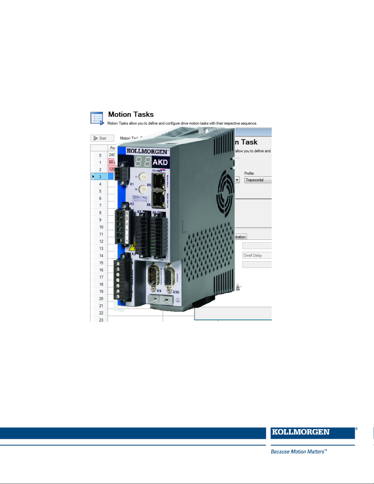
Motion Task ........................................................................................................... 16

Servo Gains ........................................................................................................... 16

Save & Print ........................................................................................................... 16

Measure ................................................................................................................. 16

Cursor .................................................................................................................... 17

Display ................................................................................................................... 17

Settings .................................................................................................................. 18

AKD™ Motion Task ..................................................................................................... 19

Homing ...................................................................................................................... 19

Home Mode Types ................................................................................................. 19

Home Type 0 ......................................................................................................... 19

Home Types 1, 2 & 3.............................................................................................. 20

Home Types 4, 5 & 6.............................................................................................. 20

Home Types 7 & 11 ............................................................................................... 21

Home Types 8, 9 & 10 ............................................................................................ 21

Home Type 12........................................................................................................ 22

Motion Task ............................................................................................................... 22

Absolute Move ....................................................................................................... 22

Relative Move ........................................................................................................ 22

Motion Task ........................................................................................................... 23

Electronic Gearing ..................................................................................................... 25

Leader .................................................................................................................... 26

Follower ................................................................................................................. 27

Tuning .......................................................................................................................... 28

Introduction ................................................................................................................ 28

Slider Tuning ............................................................................................................. 29

Bandwidth .............................................................................................................. 29

2

Slider Tuner – How it Works ................................................................................... 30

Limitations of Slider Tuner ...................................................................................... 31

Appendix A – Under Construction ............................................................................. 33

Under Construction ....................................................... Error! Bookmark not defined.

Appendix B – Under Construction ............................................................................. 35

3

Introduction to AKD™ Advanced Kollmorgen Drive™

The AKD Servo Drive is designed with the end user in mind. The AKD provides to

the customer the fastest current and velocity loops on the market. The WorkBench

graphical user interface, or GUI, makes setup fast and intuitive.

Kollmorgen servomotors with intelligent feedback devices become Plug & Play,

removing the need for any motor setup. Tuning can be completed using either the

Automatic mode or Manual mode. The Bode Tool can provide important information

about the system to which the drive is connected.

Features of AKD

• Ease of Use

• Plug & Play motor combinations

• Advance Tuning

• Intuitive Graphical User Interface

• Fastest Current and Velocity Loop on the market

• Versatile Connectivity

• Robust Design

Benefits of AKD

• Fast Setup

• Highest Throughput

• Reduced Down Time

4

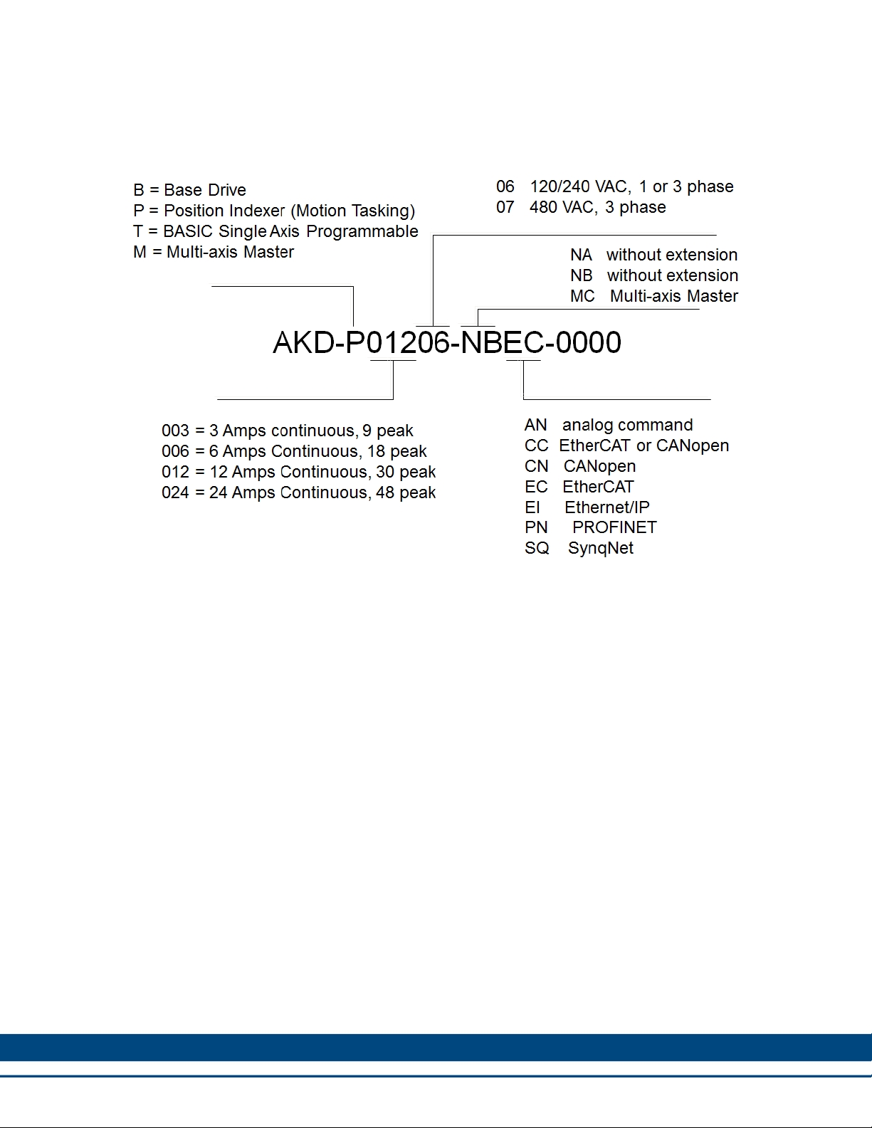
Part Number Break Down

Support Materials Available

• User Guide (in WorkBench Help)

• WorkBench & firmware

• Sample Motion Task & Setup

5

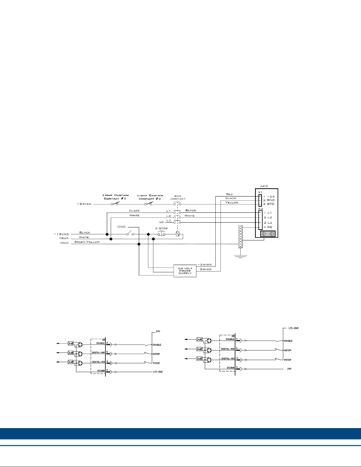
Wiring the Drive for Training

The AKD Servo Drive is mounted on the base plate and wired to 115vac for training.
The following schematic is provided since the base plate is prewired for simulation of an
electrical cabinet.

Power Connections

Include on the base plate are:

 115vac Circuit Breaker
 24vdc Power Supply
 Emergency Stop Button
 Power Contactor
 Auxiliary Contacts for STO
 Terminal Strip for easy connection
 Ground Bar

Note: Not included on the base plate are the Light Curtain Contacts. They have
been added to show where the contacts could be added in a real world
application.

The I/O connections are made using the manual control I/O box, part number: AKD­CONTROLBOX-A. The AKD I/O is Optically Isolated and can be configured for either
Sinking or Sourcing, but not both on the same connector.

Input is sourcing – Drive is sinking Input is sinking – Drive is sourcing

Note: X7 & X8 have individual DC Commons that must be wired up. These DC Commons are

not connected internally. This allows X7 & X8 to be connected as either sourcing or sinking

independently of each other. For example, X7 can be sourcing and X8 can be sinking. But all

the connections on X7 & X8 must be connected in the same configuration.

6

Digital Inputs and Outputs

The Digital I/O connections are made on connectors X7 & X8. Once the connections are
properly made, they can be configured in WorkBench. Digital Inputs 1 & 2 both are high
speed inputs with update rates of 2µs. Digital Inputs 3 to 7 are standard programmable
inputs with update rates of 250 µs.

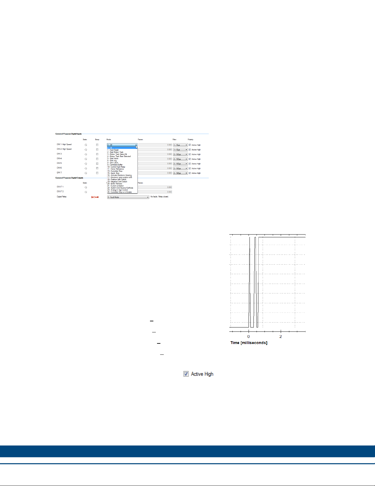
The function of the input can be programmed in WorkBench and selecting one of the
twenty-one available modes. Each input has a drop down box with the available mode.

The mode selected will depend on
the application requirements.
Keep in mind End Of Travel limits
are, in most cases, Normally
Closed, and Home Switches are
Normally Open.

All of the inputs can have Filters add, or the Polarity changed. Adding filters can be very
helpful when the input is from a mechanical switch that may bounce when closing or
opening.

Setting the filter to 0 – Off will allow all inputs to be
detected. The image to the right is a scope plot of
Digital Input 1 with filters off. The input is coming
from a snap action switch. The bounce of the
switch is clearly visible in the scope plot.

A bouncing input can trigger more than one move.
Adding a filter can insure the trigger will be
acknowledged only once.

The available filters are:

 0 – Off (detects all inputs >40ns wide)

 1 - 10µs (detects all inputs >10.24µs wide)

 2 – 162µs (detects all inputs >163µs wide)



3 – 2.62ms (detects all inputs >2.62ms wide)

Digital Input with filters off.

Polarity allows the input to be changed from Active High to Active Low. Polarity can be
changed in Workbench by clicking Polarity, , or by setting the parameter. The
parameter is, DINx.INV, and will be set as follows.

 0 – Input is Active High
 1 – Input is Active Low

CAUTION: Changing the Polarity with the drive enabled can cause unexpected motion.

7

WorkBench - AKD™ Positioner

Overview

The Advanced Kollmorgen Drive is the most advanced servo drive on the market. The
WorkBench software used to set-up and program the drive is an intuitive graphical user
interface. The power of the AKD comes for its high level features such as:

• Plug-and-Play compatibility with Kollmorgen motors

• Digital Signal Processor Control

• Optically Isolated I/O

• Highest Current Loop & Velocity Loop Bandwidth

• Fastest Digital Current Loop on the market

• Wide Feedback Range

• Multiple Bus choices

The AKD is a powerful, yet easy to set-up and use, digital servo drive. Its compact
design makes it the industry leader in power density.

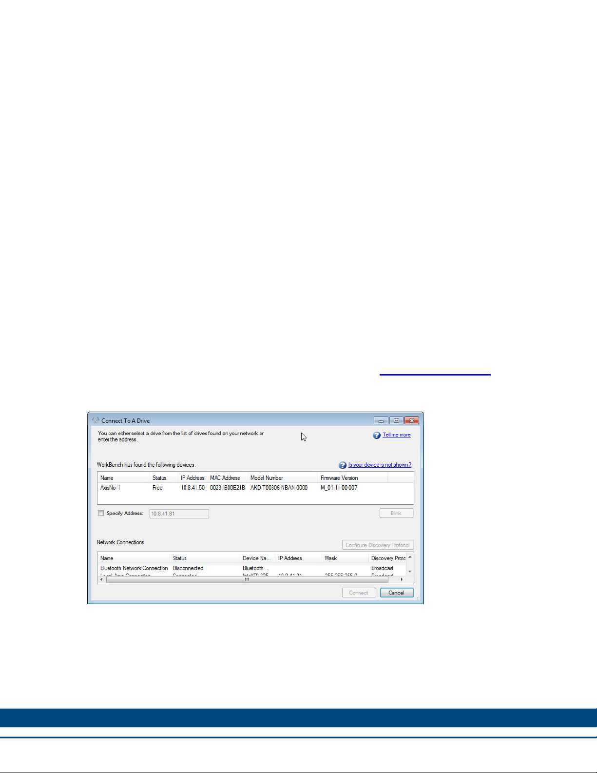
Connect to the AKD Drive

To communicate the AKD Servo Drive, the WorkBench graphical user interface is
provided. The most recent released version can be found at: www.kollmorgen.com.
The current versions of Workbench are compatible with the AKD and AKD BASIC.

Open WorkBench™.

8

IP Address

In order to use the AKD, you must be able to communicate with the device using
WorkBench and an Ethernet connection. The AKD uses TCP/IP. Both the AKD and the
PC must connect through this standard in order to communicate.

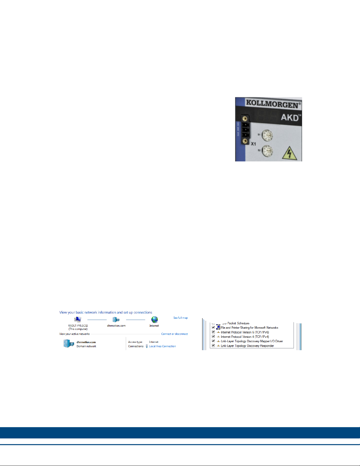
Automatic (Dynamic) IP Address

The IP Address for each drive can be set automatically, or
dynamically. This is using the Dynamic Host Configuration
Protocol (DHCP). To set the drive to Automatic IP Address
set switches S1 and S2 to 0. Either power the drive up or
cycle power.

The drive will display an I-P on the display followed by the
address. This address can change each time the logic
power is cycled.

Static IP Address

A Static (fixed) IP Address can be set using rotary switches S1 and S2. The IP address
for the drive will be set to 192.168.0x1x2. The last two numbers, x1 and x2, are set by
S1 and S2.

Example:

We want to set the drive address to reflect its location in the system. This drive
is Axis No. 15.
S1 is set to 1 & S2 is set to 5
The IP address of the drive is now: 192.168.015

For your computer to see the drive it must be setup in the same domain. To set your
computer up, go into your control panel. Here you will find either Local Are Connection
or Network and Sharing Center. If it is Network and Sharing Center enter this to find
Local Area Connection. Note that your screen may look differently depending on your
version of Windows.

In the Local Area Connection click, on Properties then scroll down to TCP/IP version 4
and click on Properties again. Set Use the following IP address and enter:
IP Address: 192.168.0.100
Subnet mask: 255.255.255.0
Then click OK.

At this point the drives IP Address will appear in the screen and the PC can connect to
drive. This address will not change until you decide to make a change.

9

WorkBench Help

parameter, Units, Range, and Data Type.

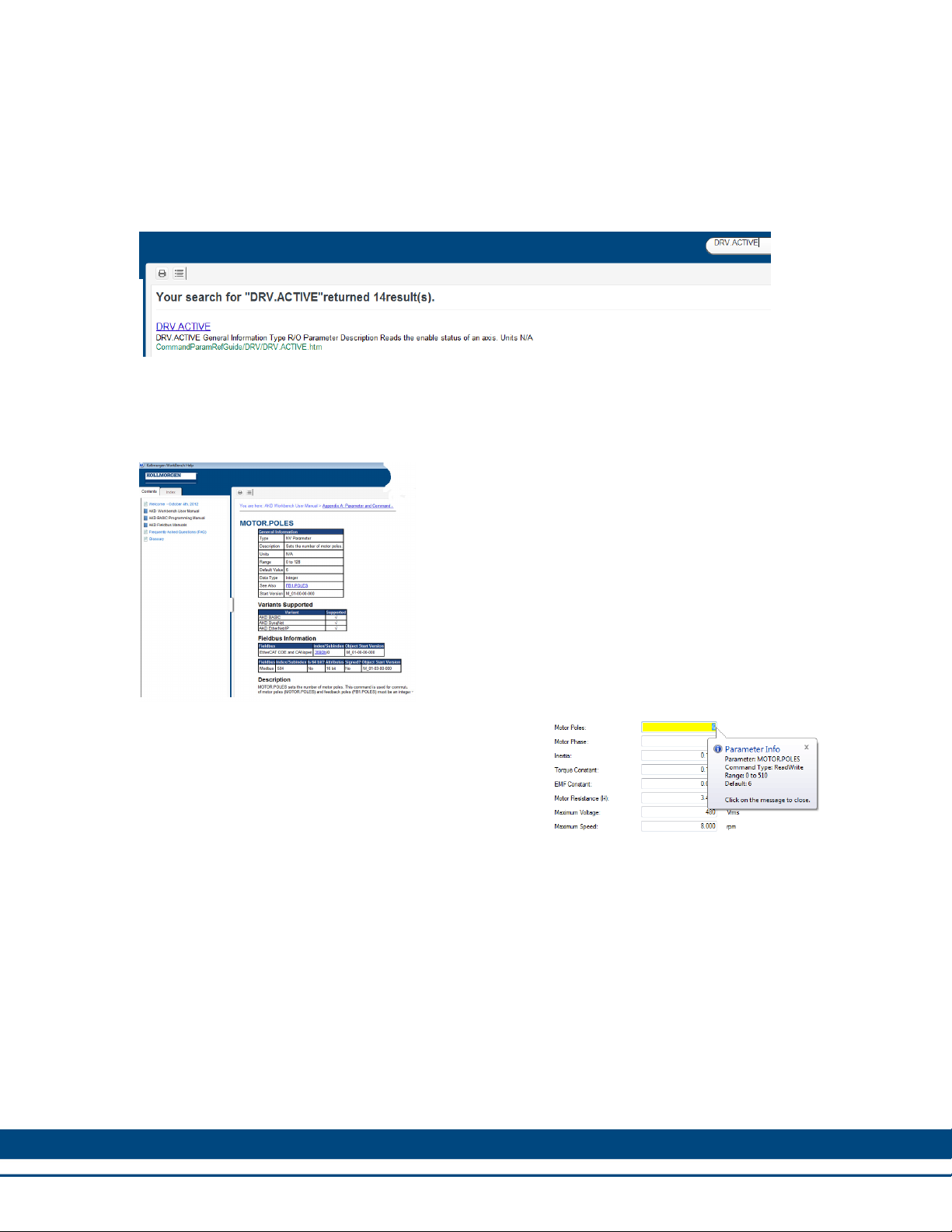
Within WorkBench is provided quick access to the help screens. These can be
accessed using the Help tab, or the F1 key. If the Help tab is used the search screen
within Help will allow you search on a specific topic. In the example a search of
DRV.ACTIVE was made returning 14 results.

Using the F1 key can take the user to a specific section by clicking on the screen, or
within a specific parameter to narrow the search. For example, from the Motor screen
and clicking in the Motor Poles then F1 brings up the Help screen specific to
MOTOR.POLES, the parameter name.

At this point all the general information about
this parameter is displayed. Some of the
important information displayed is Type of

Also include is the Variants Supported which
is helpful if the parameter is to be changed in
other drive types. The Fieldbus Information
provides the format and for this parameter in
EtherCAT COE, CANopen, and Modbus. A
detailed description of the parameter is also
provided as well as Related Topics.

Another helpful feature is using the Right Click in
the parameter box. A drop down box will appear
in which is the selection, “Parameter Info” is
available. When this is click a box with a brief
description about parameter will appear. At times
this is enough information to help complete the
current setup task.

Drive Setup Screens

Drive Overview

Settings

• Motor • Units

• Feedback 1 • Modulo

• Feedback 2 • Limits

• Brake • Home

10

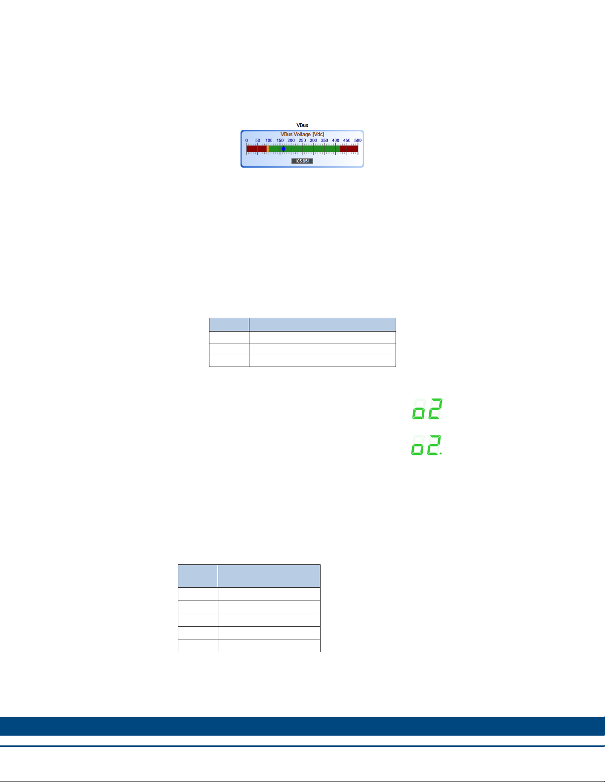
Power

The Power screen allows the bus voltage to be monitored, the DC-bus Over-Voltage
threshold, DC-bus Under-Voltage threshold, Under-Voltage Fault Mode, and the
Operating voltage.

Opmode/Source/Enabled/Running

DRV.OPMODE

The AKD™ servo drive has three operation modes in which it can function. The
operation mode, or DRV.OPMODE, of the drive is selected for the application in which
the drive is being used. The “Opmode” ranges are 0 to 2.

Mode Description

0 Current or Torque mode
1 Velocity mode
2 Position mode

The display is indicating that the drive is in position
mode and not enabled.

The display indicates that the drive is in position
mode and the drive is enabled and active.

DRV.CMDSOURCE

The Command Source sets the method with which the drive will be communicated.
During setup of the drive the command source is usually set to 0 for Service mode.

Value Description

0 Service/TCP/IP
1 Fieldbus
2 Electronic Gearing
3 Analog
5 Program

DRV.CMDSOURCE 5 is only available in the AKD BASIC servo drive and is used in the
programming mode.

11

The command source can be changed from the Workbench setup screen, or from the
terminal screen.

If the DRV.CMDSOURCE is changed in the terminal screen while the drive
is enabled the system can experience a step change in command. This can result in
unexpected motion.

The AKD™ servo drive has to two states when operating. The drive can be enabled or
disabled. This is displayed by two LED’s located on the front of the drive, and in GUI.

There times that the drive can be enabled but not active. For the drive to be active both
the Hardwar enable, HW, and Software enable, SW, must be true, and no faults can
have occurred.

The diagram above is the Boolean representation for DRV.ACTIVE to be true. There
are no faults and the Software Enable (SW) and Hardware Enable (HW) are true.

Below the DRV.ACTIVE is false and the Power Stage is off. Missing are the Software
Enable (SW) and Hardware Enable (HW).

12

Units / Terminal / Watch window / Scope Tool

Units

The Units screen is used to set the three primary drive parameters of acceleration,
velocity and position into user defined application specific units. This will allow the user
to work in clear understandable units. Motion Task will reflect the units as they are
established in this section.

For a motor only we can still set the units to our desired values.

In this example the position units are set to
degrees of the motor shaft, velocity is in RPM
(Revolutions Per Minute) of the motor shaft, and
acceleration is being set to RPS/s (Revolutions
Per Second per Second).

The range of available units allows the system to
duplicate any mechanical scenario found in
industry.

For a motor connected to a lead/ball screw with a lead of 0.5 inches/revolution of the
screw, we can set up our units as follow.

In our example the motor is connected to
the screw directly. The input has be set to
turns to show that this can be expressed
as a turns 1 to 1.

The Lead is set to 0.5”/rev of the motor.

Velocity will be in Inches/second, and acceleration
will be in Inches/second/second.

Workbench provides many examples of
mechanical devices. Each one has a
pictorial of the device to assist the operator
to correctly enter the information.

The gear ratios are entered the same way
for each unit. Either as none, Turns, or
Teeth.

Position units are set the mechanics of the
device. Since our lead screw was defined
in inches, the position will be provided in
inches as well. Also velocity and
acceleration will be mechanically
dependent.

13

Terminal

Terminal Screen allows parameter or command to be check and entered directly
from the drive and to the drive. In most training sessions the terminal screen will be the
first stop. From here the drive can be set back to factory defaults.

Note: It is important to make sure you back up the parameter files before resetting the drive as all
values will be overwritten.

DRV.RSTVAR will restore the drive to its
default values. As you begin typing the
parameter into the terminal screen it will
begin to auto fill. To the right will be a
short explanation of the parameter or

F1 can be used at any time in any screen. This will be the fast way to the help section of
Workbench. While in the terminal screen hitting F1 will take you the section on the
Terminal Screen.

Watch Window

The watch window allows selected parameters to be view in real time such as the
VL.FB, or the velocity feedback of the motor. The watch window can be turn on in three
different ways. The first is from the View tab at the top-left of Workbench.

command.

From the tree:

View-

- Toggle Watch Pane

At the bottom of Workbench will appear the Watch Window. In the example below we
are monitoring Position Feedback (PL.FB), Current Feedback (IL.FB), Velocity Feedback
(VL.FB), and the state of Digital Input 1 (DIN1.STATE).

If more than one drive is connected to Workbench Device can be setup for additional
axis and different Parameters can be set for each. This provides a simple solution to
monitor the different elements of motion.

While the watch window is providing the parameter information in real time, it is not
recorded and cannot be played back or viewed at a later time.

Ctrl +W will open and close
the watch window. Or the
Icon of the glasses can be
clicked to alternate between
open and closed.

14

Scope Tool

The Scope tool allows the user to collect and view six channels of data from the
drive. Using the trigger mode will allow data to be collect at the same points in a move
when repeated.

In the Scope Tool, Channels allows the selection of parameters to be monitored,
displayed, and saved for later recall. Parameters can be selected from the Source
section. Clicking in the box will bring up a list of parameters. Below we see the default
parameters: Current Feedback (IL.FB), Velocity Command (VL.CMD), and Velocity
Feedback (VL.FB).

Clicking in the Source section will pull up a list of standard parameters that can be
select. Not all the parameters available are on the list so an <User Defined> parameter
is available.

Time-base and Trigger allow the Recording time and
Trigger to be setup. The Recording time can be set by
simply adjusting the time in milliseconds. If, however,
there is a need to increase the number of samples within
a given time the button can be click to provide
access to the Sampling frequency and Number of
samples.

The Trigger is used to begin the recording at the same
place in the move every time. The most common
Trigger Type is VL.CMD. Since a position move will
generate a velocity command, VL.CMD, it is a very good
trigger point. The level is set slightly above the ambient
velocity command, or that which holds position.

The slope indicates the direction of the command off which the trigger will occur. If our
first move is positive this will be set to 1-Positive, and if negative it will be set to 0­Negative. Position is the amount of record time that will be kept in advance of the
trigger. When the system is armed it basically recording data at that point and will keep
the amount of data based on the Position time.

Service Motion

Service Motion allows a move or motion to
be created from the scope screen. This
can be very useful during the tuning or
troubleshooting process. The motion can
be a single pulse, Reversing motion, or a
continuous move.

15

Motion Task

From the scope screen a motion task can
be called. Using the motion task in the
scope will allow the exact motion required
for the application to be triggered and
captured. A plot of the motion task can
show any problems in the motion that may
be occurring.

Servo Gains

Servo Gains, Observer, All Gains, and AR Filter will be addressed in another class. All
of these can be seen from the scope screen and changed to improve the system
performance. As always, care should be taken when changings gains and filters as
systems can become unstable.

Save & Print

After a scope plot has been taken it may
be important to share the scope plot with
your colleagues commissioning purposes,
troubleshooting or bragging right.

The scope plot can be saved as an image
in BMP, JPG, PNG, EMF or WMF format.

The plot can also be saved in a csv (Comma Separated Values) file format which will
allow the data points to be brought into an Excel Spread sheet. This can be very useful
when evaluating the data collected.

The scope plot can also be sent to a print to create a hard copy. Associated with the
print tab is the Page Setup tab which allows the page to be set to the most practical
format for display. For example, Landscape or Portrait.

Measure

The measure tab allows basic information to be displayed. The data displayed is that
set in the Channels tab and will indicated the Average, Minimum, Maximum, Peak to
Peak, and RMS values. The data will be displayed in the units set for the system.

The average value is based on the sum of the data points divided by the number of data
points. The minimum and maximum values are the highest and lowest data points. The
Peak to Peak value is the value from the minimum to maximum values.

RMS (Root Mean Square) is the geometric average of the value.

16

Cursor

To measure the values between two points the
cursor can be used. The left Right Cursors can
be moved to their positions and the distance
between them in Time and the set units can be
displayed.

In the example the left cursor is set on the rising
edge of the digital input 1 state. The right cursor
is set at the end of the last motion task before the
return move. Between the two cursors is the
measured time, Position, Velocity Commanded
and Velocity.

We can see from the measured data that the move time is 1,065.000 milliseconds, or
approximately 1 second.

Since the motion task is set to move out 1,550 degrees and returning to zero, the
position is measure just before the return move. If it was measured after the return
move it would read approximately zero. We measure the distance moved as 1,549.581
degrees.

Display

The Display tab allows adjustments to the displayed data to make the interpretation of
the data easier. Controls allow the viewer to zoom In and Out, Pan Left and Right,
display the current data along with the last three.

The legend can be removed, the Font enlarged, Horizontal and Vertical grids added or
removed, and a Zero Line displayed. The data points can be marked as well, but with a
large number of data points the display can be cluttered.

Show Data will display the individual data points and their magnitude.

Zoom Out All will return the display to its original state.

17

Settings

Settings allows for a series of Preset Scope settings to be created. These settings can
be retrieved and used as needed.

Clicking on the Reload Current tab will bring down the list of preset scope settings.
Loading a preset will set the Channels to be recorded, the recording time, triggers etc.

The preset scope settings can be exported to the computer’s memory and shared as you
would any other file. Files can also be Imported and used. This is very helpful during
long distance troubleshooting where the data being collected will need to be as close as
possible.

18

AKD™ Motion Task

Homing

Before a position move can be executed, the home position must be established.
Workbench provides fifteen different methods to home a system and the type selected
will depend on the application and mechanics to which the motor is connected. Each
home mode provides flexibility when working with the application.

To select the proper home mode, HOME.MODE, will require an understanding of the
application. If the application does not require a known starting point, such as the case
for a conveyor that must index a set distance on a trigger, then a simple home type can
be used. Home mode 0, “Home using current position”, can be used. This will basically
allow the current position to be the starting point.

Mode Description
0 Home using current position
1 Find limit input
2 Find limit input then find zero angle
3 Find limit then find index
4 Find home input, including hardware limit switches
5 Find home input then find zero angle, including hardware limit switches
6 Find home input then find index, including hardware limit switches
7 Find zero angle
8 Move until position error exceeded
9 Move until position error exceeded, then find zero angle
10 Move until position error exceeded, then find index
11 Find index signal, without any precondition
12 Homing to a home-switch, including mechanical stop detection
13 Home using the feedback position
14 Find home input – Only in given direction

Home Mode Types

The home mode types can be broken into: use current position, find the limit switch, find
the home input, move until position error exceeded, and find zero angle or index. Each
of these can be modified to provide an offset from the home position.

Home Type 0

Mode Type 0, use current position, will make the current position the home point.
Although a very basic home type, it can be modified using Offset and Position. This
means the current position doesn’t have to be defined as zero, but can be given any
desired position, and the load can be moved from this position.

Mode Type 0 is very useful when you have a device that is not concerned with the actual
starting point such as a conveyor that will index a defined distance once an input has
been triggered. In other words, where it is beginning is not as important as where it is
going.

19

Home Types 1, 2 & 3

Using Mode types 1, 2, and 3 we see that this is basically looking for the limit input, or
End-Of-Travel switch (EOT). Modes 2 and 3 have the added “… then find zero angle”
and “… then find index.” Each feedback device will have either the zero-angle or the
index. SFD, EnDat Sine Encoder, BiSS, and Resolver will have the zero-angle. The
incremental encoder with and without Halls will have the index. These are precise
positions in the feedback device that do not change unless the motor or feedback is
changed.

Home Types 4, 5 & 6

Using Mode Types 4, 5, and 6 will be looking for a dedicated input specifically for the
Home Reference. This input can be a snap action switch, which is inherently inaccurate,
or a non-contact type switch such as Hall Effect, Inductive Proximity, Capacitive
Proximity, or Photo-detector Proximity switch. As with Mode Types 1, 2, and 3, finding
the Home Reference input can increase the accuracy by adding the zero-angle or index.

Homing to a limit switch, home input switch, or a physical hard stop can provide a
position that may fluctuate depending on the switch type, ambient temperature, or other
environmental or material changes. For example if the machine is using home mode 8,
which will drive the mechanical components into a hardstop, and the hardstop is a piece
of rubber the position will change with temperature as the rubber softens or hardens.

To remove this inaccuracy due to temperature, the load can move to the hardstop then
move off to the zero angle or index of the feedback device. This will make the homing
very repeatable.

In most cases when homing to a limit switch or hardstop an offset is desired. The Home
setup screen provides for this offset. The example below is for homing to a limit switch
with an offset.

Homing Example:
Units have been setup for connection to a
Lead Screw. The lead is 0.5”/rev. The
Position Unit is 3-Custom (mechanics
dependent) which will provide position in
inches when Custom Position Unit is set to
inches; Velocity Unit 3-Custom (mechanics
dependent) which be in inches/second;
Acceleration Unit is 3-Custom (mechanics
dependent) which will be in inches/s².

For this example the load will be homed in the negative direction, a 1-inche offset will be
provided, and the final position will be zero.

20

Velocity, Acceleration, and Deceleration
have been set to moderate values. The
Home Mode is set to type 3-Find limit
input then find index (feedback is
incremental encoder). The direction is
set to 0-Negative; this will allow the
moves to be positive from home. The
position is set to -1, and distance is set to

1. This means when the limit switch is
found the system will move off to the
index position. This point is now defined
as -1, then the system will move positive
1 inch. The Position Feedback now
reads 0.00 inches.

When homing to a limit switch the switch must be made long enough for the
system to decelerate to zero and the switch still triggered. The switch can be overshot if
the deceleration rate is very low and velocity is very high. A homing error will occur.

Home Types 7 & 11

Home Types 7 and 11 are very similar. Both use the feedback device’s internal
reference point for homing. Homing using the zero angle or index and adding an offset
can be used with each of the other Home Modes.

Home Types 8, 9 & 10

Home Types 8, 9, and 10, Move until position error exceeded, are commonly called
Homing to a Hard-stop. Basically the current will be reduced to prevent damage and
the load will be moved in one direction or another until the position error increases above
the set value. Care needs to be taken to prevent damage of the mechanical system.
The Peak Current limit set in the Homing screen needs to be high enough to overcome
all frictions in the system, yet low enough to not damage the components.

A common mistake when using Home Modes 8, 9, & 10 is to have an offset move in the
same direction as the home direction. For example using Direction: 0-Negative and
Distance: -1. Since the system was moving in the negative direction when it
encountered the hardstop, it cannot move -1 as this will be beyond the hardstop. The
system will generate an Error as seen below.

21

Home Type 12

Home Type 12, Find home input (account for mechanical end stops) will allow a system
to travel to a hard-stop, turn around, and continue looking for the Home Reference input.
This home type removes the need for adding End Of Travel limit switches to the system.
It is important to be aware that this system works similar to the Home Types 8, 9 and 10,
except the hard-stop is the EOT. Peak Current will need to be reduced enough to
prevent damage, but high enough to overcome frictions in the system.

Motion Task

In many applications point to point moves are all that is needed. AKD and
Workbench can allow simple to complex profiles to be entered into the drive and moves
triggered by the I/O.

There are two basic types of move available in the motion task. These are Absolute and
Relative moves. While both are motion types, when and how they are used is
application dependent.

Absolute Move

Absolute moves are excellent when working in a finite space such as an actuator. Since
the travel is limited to the length of travel in the actuator, Absolute moves help prevent
an accidental move beyond the travel limits.

If the systems begins at 0 degrees and an absolute move is commanded for 360
degrees, the system will move to that point. There is only one point that is 360 degrees.
If the move is repeated two more times the system will not move since it is already at

360.

Relative Move

Relative move, or Incremental move, is based on making a move of a certain distance.
The starting point is irrelevant, since the move is starting from whatever point it is
located at the time the move is initiated.

If the system begins at 0 degrees and a command to make a relative move is given the
system will move to 360 degrees. If the command is given two more times the system
will make two more moves each equaling a distance of 360 degrees. The final position
is 1080 degrees.

22

Relative moves are used in applications were the system can make repeated moves
without coming to the end of travel such as indexing tables or conveyor systems.

A clear understanding of Absolute and Relatives is required to insure that the correct
move type is used in the application. As we can see from the two examples, if
connected to an actuator with a travel limit of 360 degrees, the Relative move would
have found the end of travel and possibly damaged the actuator.

Motion Task

There are two ways create a motion task. The first is to enter the data into the
data spreadsheet. Below we see that a move of 360-degrees at 1000-rpm has been
created. The spreadsheet can be expanded to the right to add the column for the
Following Task, which is the task that will be executed after the current task, the Start
Condition and Dwell Time if the Start Condition calls for a Dwell between the Motion
Task.

The second method is to double-click the Motion Task number which will bring up the
Motion Task screen. The Motion Task screen is for a single task. It provides a visual
representation of the move and allows all the parameters to be edited in one place.

The type of move can be selected as:

Absolute
Relative to command position (PL.CMD)
Relative to previous target position
Relative to feedback position

The units for Position, Velocity, Acceleration,
and Deceleration are defined in the Units
Screen. It is important to set the Units
appropriately for the application.

Following Task is the task to be completed
after this Motion Task. They do not need go in
order and jump around as needed.

One move can blend into the next as defined in drop down section. One task can blend
into the acceleration or velocity of the next task. Scope plots of each Blend type can be
found in Appendix A.

23

Exercise

Objective: to create a series of motion task connected together using different start
conditions and blending that will be trigger from an I/O condition and captured using the
Scope tool.

Setup the following motion task all of which will Absolute moves, Trapezoidal Profiles,
and Acceleration /Deceleration 10,000 rpm/s:

Task No. Position (degrees) Velocity (rpm) Next Task Start Condition Dwell Time

0 1200 300 1 Dwell Time 250
1 2400 600 2 Dwell Time 250
2 3600 1200 3 Dwell Time 250
3 0 2000 none

Set the scope to record VL.FB, PL.FB, and DINx.STATE for the digital input selected to
start the motion task. In example, digital input 1 will be DIN1.STATE.

Set the scope to record 2.5 seconds of data, while triggering off the velocity command
going greater than 5 rpm. Remember to set the slope to 1 – Positive to catch the rising
edge. Arm the scope then trigger the motion task.

The example below is similar to what you should have displayed. The shape of the
move profiles may vary due to tuning and load. The blue line is the digital input that
triggered the move. The red line is the velocity profile for the moves. The green line is
position during the moves.

24

PLS – Programmable Limit Switches

To connect the states to the OR gate, the box must be
checked. The state indicator will illuminate when that point
is true, and will not be illuminated when not true.

PLS.EN enables the programmable limit switch. The range is 0 to 255, and is a binary
representation of the 8 programmable points. PLS.EN 255 will be for all points on, while
PLS.EN 0 is for all points off. Any combination of points can be enabled based on the
binary value of PLS.EN. PLS1 is the least significant bit, and PLS8 is the most
significant bit.

The above scope plot shows Digital Output 1 firing at the six set points.

25

Electronic Gearing

Electronic gearing allows two axis to be connected together digitally. Usually there is at
least two axis involved, but it is not uncommon to have several follower axis. One axis is
the Master, or Leader. The other axis, or multiple axis if more than one, is the Follower.

The AKD can be setup as either the Leader or the Follower, but not both. Each axis will
be setup individually. When using AKD connector X9, the connection will be one to one.

One to one connection means pin-1 on
one connector is connected to pin-1 on the
other connector. Pin-2 is connected to pin­2, and so on and so forth.

It is important to observe all grounding,
shielding and bonding procedures to insure
good performance of the system.

AKD connector X7 can also be used for electronic gearing. It can be used for 24 volt
signals to provide an up-down control. This commonly used when a third-party controller
is being used to deliver the signal.

It is important to note that this configuration is single ended and provides very little noise
rejection. It is very important to shield and ground the signal carrying cable.

Leader

The leader is the easier of the axis to setup. This will basically consist of setting up the
Emulated Encoder Output (EEO). The EEO is set in the Encoder Emulation screen.

Emulation Mode is the type of output
the AKD will generate. The more
common is mode 1-Output A/B with
once per rev index. This simulates
an A quad B encoder. The Emulation
Resolution is here in lines/rev.

The leader Emulation Resolution is from 0 to 16,777,125 lines/rev. Lines/rev is before
quadrature. Post is found by taking the resolution time four (lines/rev x 4 = counts/rev).

26

Follower

The Follower has a more complex setup compared to the Leader. Because the Follower
will be receiving the input, Encoder Emulation is set to 0-Input (No EEO Output).

The Follower Axis will be setup for the example below. The connection will be from X9
to X9 through a 9-pin Sub-D female-to-female cable. The cable is shielded and the
shield is tied to ground.

Feedback 2 will be setup for X9.
Feedback mode is 0-Input A/B Signals.
Resolution is set to 262,140 counts/rev.

The Follower must be setup for DRV.CMDSOURCE 2-Electronic Gearing. When the
command source is set Electronic Gearing an additional branch will appear on the tree.

The Input Type and Input Source will
reflect that which was set in the
Feedback 2 screen.

The ratio between the Leader and the
Follower can be set here in the In = Out
tabs. A 2:1 ratio can be set as In: 2,
Out: 1, or In: 200, Out: 100, or any
combination that will be equal 2:1. This
flexibility becomes helpful when ratios
such as 15.5:1 are required. The
values for In and Out must be integers,
so this will be set as In: 155, Out: 10.

While In (GEAR.IN) has a range of 1 to 65,535, Out (GEAR.OUT) has a range from

-32,768 to 32,767. Since Out can be negative it can be used to counter rotate two axis,
or correct for axis in which one motor is mounted opposite another.

Limit can be set for the Follower axis using the Maximum Velocity, Maximum
Acceleration, and Maximum Deceleration. In most cases it is best to set Acceleration
and Deceleration as high as possible. Limiting Acc and Dec and adversely affect the
system performance.

The Gearing Type defines how gearing will start if the Leader is
already in motion. Since the electronic gearing can be used to
synchronize two axis, it should understood relationship

between the Leader and Follower.
If the follower is only meant to come up to the same speed as the Leader then Velocity
Matching will be used. Position Matching is used when the Leader and Follower need to
be lock together by their position. When engaged, the Follower will speed up and
recover the steps lost during the acceleration.

27

Tuning

Introduction

In a perfect world tuning a system would not be required. In the “Real World” tuning a
system is a necessity.

A servo system is a closed loop system which will continually monitor and adjust torque,
velocity, and position to achieve the desired trajectory. A servo system can operate in
torque mode, or velocity mode, or position mode. In the diagram above can be seen a
simplified diagram of these three loops.

The tuning begins at the right with the current loop which is tuned for the motor. The
current loops function is to insure that as much current as possible can get into and out
of the motor as quickly as possible. The current loop does take into account the load
and doesn’t even care if a load is connected or not.

The velocity loop is added to the current loop. The velocity loop is tuned after the
current loop and is tuned specifically for the load. The tuning is basically telling the drive
how it needs to react to any change in velocity. If the load is very small, JL/JM=1:1 or
less, a slight change in velocity does not warrant a huge injection of error into the system
to correct for this change.

At the other end of the spectrum is a large load, JL/JM =1,000:1. Since the load will
create a large opposition to motor, a larger error will need to be injected into the system
to insure enough torque is generated to overcome the load and correct the change in
velocity.

The position loop can be added to the velocity loop and current loop after they have
been tuned. The position loop is now monitoring the position as well as velocity and will
need to be tuned for the load for the same reasons the velocity loop is tuned for the load.

The AKD provides several paths for tuning the system from the Slider Tuner to the
Performance Servo Tuner which can tune in Automatic Mode or Manual Mode. Accept
for the most extreme cases, the AKD can be tuned to provide excellent performance with
high inertial loads, systems resonance, and poor mechanical components.

The Key to good servo performance is to begin with a sound mechanical system!

28

Slider Tuning

The slider tuner is a simple easy to use tool that can get most servo systems up and
running in just a few minutes. It requires two pieces of information:

Load inertia

Bandwidth

The desired bandwidth can be entered by using the gentle/medium/stiff settings which
represents 25Hz, 75Hz, or 200Hz respectively. You can also type in the desired
bandwidth, or use the slider bar itself to increase the value.

The “More>>” button opens the screen to identify what specific gains are being set, and
to what values.

Important Notes: The slider tuner does modify one of the digital filters (Biquads) and
tunes a low pass filter based on the bandwidth selected. It is important to keep track of
any filters that are present to maintain stability. The Slider tuner does not configure any
feed-forwards (current, friction, velocity, acceleration, etc.). Manual set up may be
required to optimize motion profiles.

What Bandwidth is required?

The simple answer is based on just how fast you need the system to settle from
disturbances or motion. Knowing your desired settling time allows you to calculate your
system bandwidth:

System Bandwidth = 1/Settling Time (seconds)

Desired bandwidth

29

Slider Tuner – How it Works

How does the slider tuner know what the tuning gains should be just from the bandwidth
and load inertia? Slider tuner will set four parameters, VL.KP (velocity proportional gain),
VL.KI (velocity integral gain), PL.KP (position proportional gain), IL.KP (current
proportional gain), and one biquad filter, AR1. Let’s look at each one individually:

First – VL.KP, or Velocity Proportional Gain

ܸܮ.ܭܲ = 2ߨ∗ܤܹ∗ܬܯ∗(1+ܬܮ)∗0.0001*ܭݐ

JM and JL are in units of kg-cm2, BW in in Hz, and Kt is N-m/A

rms

VL.KP will bring the gain of the system up to a specific performance rating (bandwidth).
Therefor it is based on how strong the motor is (Kt – the motor torque constant) and how
much mass is attached to the motor (JM – motor shaft mass and JL – load mass).

Next we look at VL.KI, or Velocity Integral Gain

VL.KI = BW * tan(2.5°)

BW and VL.KI are in units of Hz

There is no standard to how much velocity integral gain is needed on a system. The
slider tuner makes a conservative assumption and sets the Velocity Integral gain to
contribute only 2.5 degrees of phase loss at the bandwidth requested.

Next, we look at PL.KP, or the Position Proportional Gain

PL.KP = BW * tan(2.5°) * 2π

BW is in units of Hz, PL.KP is in (rev/s)/rev (can be converted to Hz by dividing by 2ߨ)

The required Position Proportional gain will also vary from system to system. The slider
tuner sets the Position Proportional gain to contribute only 2.5 degrees of phase loss at
the bandwidth requested.

Our next parameter is IL.KP, or the Current Proportional Gain.

IL.KP = IL BW * tan(2.5°) *2π * Motor Inductance (mH)

Where BW is in units of Hz

First a current loop bandwidth must be calculated:

IL BW = 75 Hz / tan 5 = 857 Hz

30

Next, IL BW (Current Loop Bandwidth) is clamped between 1000 Hz and 2000 Hz to

݂݂݂݂

݅݅݅݅

݈݈݈݈

ݐݐݐݐ

݁݁݁݁

ݎݎݎݎ

ܨܨܨܨ

ݎݎݎݎ

݁݁݁݁

ݍݍݍݍ

ࢎࢎࢎࢎ

ݖݖݖݖ

====

((((

−(

−(−(

−(

܋܋܋܋

ܗܗܗܗ

ܛܛܛܛ

݌݌݌݌

૛૛૛૛

∗∗∗∗

ܾܾܾܾ

ݓݓݓݓ

૝૝૝૝

−−−−

૝૝૝૝

∗∗∗∗

ܾܾܾܾ

ݓݓݓݓ

૛૛૛૛

∗∗∗∗

૞૞૞૞

૙૙૙૙

૙૙૙૙

૙૙૙૙

૛૛૛૛

++++

૞૞૞૞

૙૙૙૙

૙૙૙૙

૙૙૙૙

૝૝૝૝

−−−−

૛૛૛૛

∗∗∗∗

ܛܛܛܛ

ܑܑܑܑ

ܖܖܖܖ

݌݌݌݌

∗∗∗∗

܋܋܋܋

ܗܗܗܗ

ܛܛܛܛ

݌݌݌݌

∗∗∗∗

ܾܾܾܾ

ݓݓݓݓ

∗∗∗∗

ܾܾܾܾ

ݓݓݓݓ

૛૛૛૛

−−−−

૞૞૞૞

૙૙૙૙

૙૙૙૙

૙૙૙૙

૛૛૛૛

∗∗∗∗

૞૞૞૞

૙૙૙૙

૙૙૙૙

૙૙૙૙

∗∗∗∗

૛૛૛૛

++++

૛૛૛૛

∗∗∗∗

((((

ܾܾܾܾ

ݓݓݓݓ

૝૝૝૝

−−−−

ܾܾܾܾ

ݓݓݓݓ

૛૛૛૛

∗∗∗∗

૞૞૞૞

૙૙૙૙

૙૙૙૙

૙૙૙૙

૛૛૛૛

++++

૞૞૞૞

૙૙૙૙

૙૙૙૙

૙૙૙૙

૝૝૝૝

))))

−−−−

܋܋܋܋

ܗܗܗܗ

ܛܛܛܛ

݌݌݌݌

∗∗∗∗

ܾܾܾܾ

ݓݓݓݓ

૛૛૛૛

−−−−

૞૞૞૞

૙૙૙૙

૙૙૙૙

૙૙૙૙

૛૛૛૛

−−−−

ܛܛܛܛ

ܑܑܑܑ

ܖܖܖܖ

݌݌݌݌

∗∗∗∗

ܾܾܾܾ

ݓݓݓݓ

∗∗∗∗

૞૞૞૞

૙૙૙૙

૙૙૙૙

૙૙૙૙

∗∗∗∗

૛૛૛૛

))))

∗∗∗∗

ܾܾܾܾ

ݓݓݓݓ

૛૛૛૛

∗∗∗∗

܋܋܋܋

ܗܗܗܗ

ܛܛܛܛ

ܘܘܘܘ

∗∗∗∗

܊܊܊܊

ܟܟܟܟ

∗∗∗∗

૞૞૞૞

૙૙૙૙

૙૙૙૙

૙૙૙૙

−−−−

ܛܛܛܛ

ܑܑܑܑ

ܖܖܖܖ

ܘܘܘܘ

∗∗∗∗

܊܊܊܊

ܟܟܟܟ

૛૛૛૛

−−−−

૞૞૞૞

૙૙૙૙

૙૙૙૙

૙૙૙૙

૛૛૛૛

∗∗∗∗

૛૛૛૛

maintain numerical accuracy and stability.
IL BW = 1000 Hz

Note: Default tuning will leave the current loop with ~1000 Hz bandwidth. If manual
tuning is used to achieve more than a few hundred Hertz, IL.KP will need to be manually
increased appropriately.

Finally, AR1 is set as a low pass with a cutoff frequency calculated to cause no more
than 8.5 degrees phase loss at the requested frequency.

Yes – this is a BIG equation and very cumbersome than most would like. However,
since the slider tuner is limited over a small frequency range (no larger than 300 Hz
bandwidth), an acceptable substitute is:

AR1 Frequency = 9 * BW

Important Note: All systems are different. Integral gains can be sensitive to
mechanical oscillations and friction. The slider tuner may not be appropriate for some
applications.

Limitations of Slider Tuner

Why use anything else? The slider tuner is very simple to use as it can get simple
mechanical assemblies tuned reasonably well with little fine tuning. When mechanical
systems get beyond a simple rigid load, more tuning finesse is often required to handle
the complex resonances created by complicated mechanics.

Common systems that may not be able to be optimized using the slider tuner:

Belt driven loads High friction mechanics
Multi-staged loads (multiple resonant loads) Low resolution feedback
Linear motors Unknown inertia loads

Unfortunately, the slider Tuner won’t work for every system. This is primarily because
the slider tuner does not measure any part of your motor or mechanics and assumes the
ideal case. It also assumes the load inertia you entered includes all of your loads.
Rarely are mechanical systems ideal – there is always something unexpected like
friction, imprecise manufacturing of components, belt tensioning, and even variations
from machine to machine.

In these cases, solving advanced problems will require just a bit more work. Using the
AKD Performance Tuner feature, it is possible to measure your physical system and
tune on what is actually, physically there, even if there are variations from machine to
machine. The Performance Tuner allows you to visualize these problems and adjust
tuning accordingly.

31

Projects

Project #1 Bode Tool & Tuning

On your hard drive create a folder called: AKD Projects.

1. Take a Bode Plot of your system and save it to your project folder.

2. Set the tuning using the Slider Tuning.

32

Appendix A – Always Under Construction

Blending Moves

When a more complex move is require, moves can be connected together using the
Blend feature. The move can be connected without any blending, or blended into the
acceleration or velocity of the next move. It should be noted this will only work for those
motion task of the same direction.

250 millisecond dwell between moves. The distance, acceleration, and decelerations
are the same for the motion task, but the velocity is different. The results are three
moves with the acceleration and distance covered, but different times to complete the
move.

Motion Task 0 blended into the acceleration of Motion Task 1.

33

Motion Task 0 blended into the velocity of Motion Task 1.

34

Appendix B – Under Construction

North America

Europe

Under Construction

About Kollmorgen

Kollmorgen is a leading provider of motion systems and
components for machine builders. Through world-class
knowledge in motion, industry-leading quality and
deep expertise in linking and integrating standard and
custom products, Kollmorgen delivers breakthrough
solutions that are unmatched in performance, reliability
and ease-of-use, giving machine builders an irrefutable
marketplace advantage.

For assistance with your application needs, contact
us at: 540-633-3545, [e-mail]
or visit www.kollmorgen.com

Kollmorgen

203A West Rock Road
Radford, VA 24141 USA
Phone: [phone]
Fax: [phone]

Kollmorgen

Wacholderstraße 40 – 42
40489 Düsseldorf Germany
Phone: + 49 (0) 2039979235
Fax: + 49 (0) 20399793314

35