

Keysight Technologies InfiniiVision 1000 X Series, EDUX1002A, EDUX1002G, DSOX1102A, DSOX1102G User Manual
Page 1

Keysight InfiniiVision
1000 X-Series Oscilloscopes
User's Guide
Page 2

Notices
CAUTION
© Keysight Technologies, Inc. 2005-2019
No part of this manual may be reproduced in
any form or by any means (including
electronic storage and retrieval or translation
into a foreign language) without prior
agreement and written consent from
Keysight Technologies, Inc. as governed by
United States and international copyright
laws.
Manual Part Number
54612-97030
Edition
Fourth edition, June 2019
Printed in Malaysia
Published by:
Keysight Technologies, Inc.
1900 Garden of the Gods Road
Colorado Springs, CO 80907 USA
Print History
54612-97001, November 2016
54612-97015, February 2018
54612-97017, September 2018
54612-97030, June 2019
Warranty
The material contained in this document is
provided "as is," and is subject to being
changed, without notice, in future editions.
Further, to the maximum extent permitted
by applicable law, Keysight disclaims all
warranties, either express or implied, with
regard to this manual and any information
contained herein, including but not limited
to the implied warranties of merchantability
and fitness for a particular purpose.
Keysight shall not be liable for errors or for
incidental or consequential damages in
connection with the furnishing, use, or
performance of this document or of any
information contained herein. Should
Keysight and the user have a separate
written agreement with warranty terms
covering the material in this document that
conflict with these terms, the warranty
terms in the separate agreement shall
control.
Technology License
The hardware and/or software described in
this document are furnished under a license
and may be used or copied only in
accordance with the terms of such license.
U.S. Government Rights
The Software is "commercial computer
software," as defined by Federal Acquisition
Regulation ("FAR") 2.101. Pursuant to FAR
12.212 and 27.405-3 and Department of
Defense FAR Supplement ("DFARS")
227.7202, the U.S. government acquires
commercial computer software under the
same terms by which the software is
customarily provided to the public.
Accordingly, Keysight provides the Software
to U.S. government customers under its
standard commercial license, which is
embodied in its End User License Agreement
(EULA), a copy of which can be found at
www.keysight.com/find/sweula. The
license set forth in the EULA represents the
exclusive authority by which the U.S.
government may use, modify, distribute, or
disclose the Software. The EULA and the
license set forth therein, does not require or
permit, among other things, that Keysight: (1)
Furnish technical information related to
commercial computer software or
commercial computer software
documentation that is not customarily
provided to the public; or (2) Relinquish to, or
otherwise provide, the government rights in
excess of these rights customarily provided
to the public to use, modify, reproduce,
release, perform, display, or disclose
commercial computer software or
commercial computer software
documentation. No additional government
requirements beyond those set forth in the
EULA shall apply, except to the extent that
those terms, rights, or licenses are explicitly
required from all providers of commercial
computer software pursuant to the FAR and
the DFARS and are set forth specifically in
writing elsewhere in the EULA. Keysight shall
be under no obligation to update, revise or
otherwise modify the Software. With respect
to any technical data as defined by FAR
2.101, pursuant to FAR 12.211 and 27.404.2
and DFARS 227.7102, the U.S. government
acquires no greater than Limited Rights as
defined in FAR 27.401 or DFAR 227.7103-5
(c), as applicable in any technical data.
Safety Notices
A CAUTION notice denotes a hazard.
It calls attention to an operating
procedure, practice, or the like that,
if not correctly performed or
adhered to, could result in damage
to the product or loss of important
data. Do not proceed beyond a
CAUTION notice until the indicated
conditions are fully understood and
met.
2 Keysight InfiniiVision 1000 X-Series Oscilloscopes User's Guide
Page 3

WARNING
A WARNING notice denotes a
hazard. It calls attention to an
operating procedure, practice, or
the like that, if not correctly
performed or adhered to, could
result in personal injury or death.
Do not proceed beyond a WARNING
notice until the indicated
conditions are fully understood and
met.
Keysight InfiniiVision 1000 X-Series Oscilloscopes User's Guide 3
Page 4

InfiniiVision 1000 X-Series Oscilloscopes—At a Glance
~
Digital Storage Oscilloscope
DSOX1102AG
70 MHz 2 GSa/ s
Table 1 1000 X-Series Model Numbers, Bandwidths
Model: EDUX1002A EDUX1002G DSOX1102A DSOX1102G
Channels: 2
Bandwidth: 50 MHz 70 MHz, 100 MHz with DSOX1B7T102
upgrade
Sampling rate: 1 GSa/s 2 GSa/s
Memory: 100 kpts 1 Mpts
Segmented memory: No Yes
Waveform generator: No Yes (20 MHz) No Yes (20 MHz)
Mask/limit test: No Yes
The Keysight InfiniiVision 1000 X-Series oscilloscopes deliver these features:
• 7 inch WVGA display.
4 Keysight InfiniiVision 1000 X-Series Oscilloscopes User's Guide
Page 5

• 50,000 waveforms/second update rate.
• All knobs are pushable for making quick selections.
• Trigger types: edge, pulse width, and video on EDUX1000-Series models.
DSOX1000-Series models add: pattern, rise/fall time, and setup and hold.
• Serial decode/trigger options for: I
models. DSOX1000-Series models add: CAN, LIN, and SPI.
• Math waveforms: add, subtract, multiply, divide, FFT (magnitude and phase),
and low-pass filter.
• Reference waveforms (2) for comparing with other channel or math waveforms.
• Many built-in measurements.
• G-suffix models have built-in waveform generator with: sine, square, ramp,
pulse, DC, noise.
• USB port makes printing, saving, and sharing data easy.
• A Quick Help system is built into the oscilloscope. Press and hold any key to
display Quick Help. Complete instructions for using the quick help system are
given in "Access the Built-In Quick Help" on page 31.
For more information about InfiniiVision oscilloscopes, see:
www.keysight.com/find/scope
2
C and UART/RS232 on EDUX1000-Series
Keysight InfiniiVision 1000 X-Series Oscilloscopes User's Guide 5
Page 6

In This Guide
This guide shows how to use the InfiniiVision 1000 X-Series oscilloscopes.
When unpacking and using the
oscilloscope for the first time, see:
When displaying waveforms and
acquired data, see:
When setting up triggers or changing
how data is acquired, see:
Making measurements and analyzing
data:
When using the built-in waveform
generator, see:
• Chapter 1, “Getting Started,” starting on page 13
• "Running, Stopping, and Making Single
Acquisitions (Run Control)" on page 34
• "Horizontal Controls" on page 35
• "Vertical Controls" on page 38
• "Analog Bus Display" on page 41
• "FFT Spectral Analysis" on page 42
• "Math Waveforms" on page 46
• "Reference Waveforms" on page 48
• "Display Settings" on page 49
• "Triggers" on page 52
• "Acquisition Control" on page 56
• "Cursors" on page 63
• "Measurements" on page 65
• "Mask Testing" on page 67
• "Digital Voltmeter" on page 74
• "Frequency Response Analysis" on page 75
• "Waveform Generator" on page 77
When using licensed serial bus
decode and triggering features, see:
When saving, recalling, or printing,
see:
• "Serial Bus Decode/Trigger" on page 78
• "Save/Recall (Setups, Screens, Data)" on page 84
• "Print (Screens)" on page 87
6 Keysight InfiniiVision 1000 X-Series Oscilloscopes User's Guide
Page 7

When using the oscilloscope's utility
NOTE
functions, see:
For reference information, see: • "Specifications and Characteristics" on page 91
Abbreviated instructions for pressing a series of keys and softkeys
Instructions for pressing a series of keys are written in an abbreviated manner. Instructions for
pressing [Key1], then pressing Softkey2, then pressing Softkey3 are abbreviated as follows:
Press [Key1]> Softkey2 > Softkey3.
The keys may be a front panel [Key] or a Softkey. Softkeys are the six keys located directly
below the oscilloscope display.
• "Utility Settings" on page 88
• "Environmental Conditions" on page 92
• "Probes and Accessories" on page 93
• "Software and Firmware Updates" on page 94
• "Acknowledgements" on page 95
• "Product Markings and Regulatory
Information" on page 97
Keysight InfiniiVision 1000 X-Series Oscilloscopes User's Guide 7
Page 8

8 Keysight InfiniiVision 1000 X-Series Oscilloscopes User's Guide
Page 9

Contents
InfiniiVision 1000 X-Series Oscilloscopes—At a Glance / 4
In This Guide / 6
1 Getting Started
Inspect the Package Contents / 14
Power-On the Oscilloscope / 15
Connect Probes to the Oscilloscope / 16
Maximum input voltage at analog inputs / 16
Do not float the oscilloscope chassis / 16
Input a Waveform / 17
Recall the Default Oscilloscope Setup / 18
Use Autoscale / 19
Compensate Passive Probes / 20
Learn the Front Panel Controls and Connectors / 22
Front Panel Overlays for Different Languages / 27
Learn the Rear Panel Connectors / 28
Learn the Oscilloscope Display / 29
Access the Built-In Quick Help / 31
2 Quick Reference
Running, Stopping, and Making Single Acquisitions (Run
Control) / 34
Keysight InfiniiVision 1000 X-Series Oscilloscopes User's Guide 9
Page 10

Horizontal Controls / 35
Horizontal Knobs and Keys / 35
Horizontal Softkey Controls / 35
Zoom / 36
Vertical Controls / 38
Vertical Knobs and Keys / 38
Vertical Softkey Controls / 38
Setting Analog Channel Probe Options / 40
Analog Bus Display / 41
FFT Spectral Analysis / 42
FFT Measurement Hints / 42
FFT DC Value / 44
FFT Aliasing / 44
FFT Spectral Leakage / 45
Math Waveforms / 46
Units for Math Waveforms / 47
Reference Waveforms / 48
Display Settings / 49
To load a list of labels from a text file you create / 50
Triggers / 52
Trigger Knobs and Keys / 52
Trigger Types / 52
Trigger Mode, Coupling, Reject, Holdoff / 53
External Trigger Input / 55
Acquisition Control / 56
Selecting the Acquisition Mode / 56
Overview of Sampling / 57
Cursors / 63
Cursor Knobs and Keys / 63
10 Keysight InfiniiVision 1000 X-Series Oscilloscopes User's Guide
Page 11

Cursor Softkey Controls / 63
Measurements / 65
Mask Testing / 67
Creating/Editing Mask Files / 67
Digital Voltmeter / 74
Frequency Response Analysis / 75
Waveform Generator / 77
Serial Bus Decode/Trigger / 78
CAN Decode/Trigger / 79
I2C Decode/Trigger / 80
LIN Decode/Trigger / 80
SPI Decode/Trigger / 81
UART/RS232 Decode/Trigger / 82
Save/Recall (Setups, Screens, Data) / 84
Length Control / 85
Print (Screens) / 87
Utility Settings / 88
USB Storage Devices / 89
Configuring the [Quick Action] Key / 90
Specifications and Characteristics / 91
Environmental Conditions / 92
Declaration of Conformity / 92
Probes and Accessories / 93
Software and Firmware Updates / 94
Acknowledgements / 95
Product Markings and Regulatory Information / 97
Index
Keysight InfiniiVision 1000 X-Series Oscilloscopes User's Guide 11
Page 12

12 Keysight InfiniiVision 1000 X-Series Oscilloscopes User's Guide
Page 13

Keysight InfiniiVision 1000 X-Series Oscilloscopes
User's Guide
1 Getting Started
Inspect the Package Contents / 14
Power-On the Oscilloscope / 15
Connect Probes to the Oscilloscope / 16
Input a Waveform / 17
Recall the Default Oscilloscope Setup / 18
Use Autoscale / 19
Compensate Passive Probes / 20
Learn the Front Panel Controls and Connectors / 22
Learn the Rear Panel Connectors / 28
Learn the Oscilloscope Display / 29
Access the Built-In Quick Help / 31
This chapter describes the steps you take when using the oscilloscope for the first
time.
13
Page 14

1 Getting Started
Inspect the Package Contents
• Inspect the shipping container for damage.
If your shipping container appears to be damaged, keep the shipping container
or cushioning material until you have inspected the contents of the shipment
for completeness and have checked the oscilloscope mechanically and
electrically.
• Verify that you received the following items and any optional accessories you
may have ordered:
• InfiniiVision 1000 X-Series oscilloscope.
• Power cord (country of origin determines specific type).
• Two oscilloscope probes.
14 Keysight InfiniiVision 1000 X-Series Oscilloscopes User's Guide
Page 15

Power-On the Oscilloscope
WARNING
Getting Started 1
Power
Requirements
Ventilation
Requirements
To po wer-on the
oscilloscope
Line voltage, frequency, and power:
• ~Line 100-120 Vac, 50/60/400 Hz
• 100-240 Vac, 50/60 Hz
•50W max
The air intake and exhaust areas must be free from obstructions. Unrestricted air
flow is required for proper cooling. Always ensure that the air intake and exhaust
areas are free from obstructions.
The fan draws air in from the left side and bottom of the oscilloscope and pushes it
out behind the oscilloscope.
When using the oscilloscope in a bench-top setting, provide at least 2" clearance
at the sides and 4" (100 mm) clearance above and behind the oscilloscope for
proper cooling.
1 Connect the power cord to the rear of the oscilloscope, then to a suitable AC
voltage source. Route the power cord so the oscilloscope's feet and legs do not
pinch the cord.
2 The oscilloscope automatically adjusts for input line voltages in the range 100
to 240 VAC. The line cord provided is matched to the country of origin.
Always use a grounded power cord. Do not defeat the power cord ground.
Keysight InfiniiVision 1000 X-Series Oscilloscopes User's Guide 15
3 Press the power switch.
The power switch is located on the lower left corner of the front panel. The
oscilloscope will perform a self-test and will be operational in a few seconds.
Page 16

1 Getting Started
CAUTION
CAUTION
WARNING
Connect Probes to the Oscilloscope
1 Connect the oscilloscope probe to an oscilloscope channel BNC connector.
2 Connect the probe's retractable hook tip to the point of interest on the circuit or
device under test. Be sure to connect the probe ground lead to a ground point
on the circuit.
Maximum input voltage at analog inputs
150 Vrms, 200 Vpk
Do not float the oscilloscope chassis
Defeating the ground connection and "floating" the oscilloscope chassis will probably
result in inaccurate measurements and may also cause equipment damage. The probe
ground lead is connected to the oscilloscope chassis and the ground wire in the power
cord. If you need to measure between two live points, use a differential probe with
sufficient dynamic range.
Do not negate the protective action of the ground connection to the oscilloscope. The
oscilloscope must remain grounded through its power cord. Defeating the ground
creates an electric shock hazard.
16 Keysight InfiniiVision 1000 X-Series Oscilloscopes User's Guide
Page 17

Input a Waveform
WARNING
The Probe Comp signal is used for compensating probes.
1 Connect an oscilloscope probe from channel 1 to the Demo, Probe Comp terminal
on the front panel.
2 Connect the probe's ground lead to the ground terminal (next to the Demo
terminal).
A voltage source should never be connected to the ground terminal of this instrument.
If, for any reason, the Protective Conductor Terminal is disconnected or not functioning
properly and a voltage source is connected to the equipment's ground terminals, the
entire chassis will be at the voltage potential of the voltage source, and the operator or
bystanders could receive an electric shock.
Getting Started 1
Keysight InfiniiVision 1000 X-Series Oscilloscopes User's Guide 17
Page 18

1 Getting Started
Recall the Default Oscilloscope Setup
To recall the default oscilloscope setup:
1 Press [Default Setup].
The default setup restores the oscilloscope's default settings. This places the
oscilloscope in a known operating condition.
In the Save/Recall menu, there are also options for restoring the complete factory
settings or performing a secure erase (see "Save/Recall (Setups, Screens,
Data)" on page 84).
18 Keysight InfiniiVision 1000 X-Series Oscilloscopes User's Guide
Page 19

Use Autoscale
Getting Started 1
Use [Auto Scale] to automatically configure the oscilloscope to best display the
input signals.
1 Press [Auto Scale].
You should see a waveform on the oscilloscope's display similar to this:
2 If you want to return to the oscilloscope settings that existed before, press Undo
Autoscale.
3 If you want to enable "fast debug" autoscaling, change the channels
autoscaled, or preserve the acquisition mode during autoscale, press Fast
Debug, Channels, or Acq Mode.
These are the same softkeys that appear in the Autoscale Preferences menu.
See "Utility Settings" on page 88.
If you see the waveform, but the square wave is not shaped correctly as shown
above, perform the procedure "Compensate Passive Probes" on page 20.
If you do not see the waveform, make sure the probe is connected securely to the
front panel channel input BNC and to the Demo/Probe Comp terminal.
Keysight InfiniiVision 1000 X-Series Oscilloscopes User's Guide 19
Page 20

1 Getting Started
NOTE
Perfectly compensated
Over compensated
Under compensated
Compensate Passive Probes
Each oscilloscope passive probe must be compensated to match the input
characteristics of the oscilloscope channel to which it is connected. A poorly
compensated probe can introduce significant measurement errors.
If your probe has a configurable attenuation setting (like the N2140/42A probes do), the 10:1
setting must be used for probe compensation.
1 Input the Probe Comp signal (see "Input a Waveform" on page 17).
2 Press [Default Setup] to recall the default oscilloscope setup (see "Recall the
Default Oscilloscope Setup" on page 18).
3 Press [Auto Scale] to automatically configure the oscilloscope for the Probe
Comp signal (see "Use Autoscale" on page 19).
4 Press the channel key to which the probe is connected ([1], [2], etc.).
5 In the Channel Menu, press Probe.
6 In the Channel Probe Menu, press Probe Check; then, follow the instructions
on-screen.
20 Keysight InfiniiVision 1000 X-Series Oscilloscopes User's Guide
If necessary, use a nonmetallic tool (supplied with the probe) to adjust the
trimmer capacitor on the probe for the flattest pulse possible.
On some probes (like the N2140/42A probes), the trimmer capacitor is located
on the probe BNC connector. On other probes (like the N2862/63/90 probes),
the trimmer capacitor is a yellow adjustment on the probe tip.
7 Connect probes to all other oscilloscope channels.
Page 21

8 Repeat the procedure for each channel.
Getting Started 1
Keysight InfiniiVision 1000 X-Series Oscilloscopes User's Guide 21
Page 22

1 Getting Started
6. [Auto Scale] key5. [Default Setup] key
~
Digital Storage Oscilloscope
DSOX1102AG
70 MHz 2 GSa/ s
10. Tools keys
1. Power
switch
2. Softkeys
3. [Intensity]
key
4. Entry knob
11. Trigger controls
12. Waveform keys
19. Demo/Probe Comp
and Ground
terminals
15. Ext Trig
input
20. USB
Host
port
13. [Help] key
8. Run Control keys
9. Measure controls
7. Horizontal and Acquisition controls
16. Vertical
controls
18. Waveform
generator
output
17. Analog
channel
inputs
14. [Bus] key
Back
Back
Learn the Front Panel Controls and Connectors
On the front panel, key refers to any key (button) you can press.
Softkey specifically refers to the six keys next to the display. Menus and softkey
labels appear on the display when other front panel keys are pressed. Softkey
functions change as you navigate through the oscilloscope's menus.
For the following figure, refer to the numbered descriptions in the table that
follows.
1. Power switch Press once to switch power on; press again to switch power off. See "Power-On the
2. Softkeys The functions of these keys change based upon the menus shown on the display next to the keys.
3. [Intensity] key Press the key to illuminate it. When illuminated, turn the Entry knob to adjust waveform intensity.
Oscilloscope" on page 15.
The Back key moves back in the softkey menu hierarchy. At the top of the hierarchy, the
Back key turns the menus off, and oscilloscope information is shown instead.
You can vary the intensity control to bring out signal detail, much like an analog oscilloscope.
22 Keysight InfiniiVision 1000 X-Series Oscilloscopes User's Guide
Page 23

Getting Started 1
4. Entry knob The Entry knob is used to select items from menus and to change values. The function of the Entry
knob changes based upon the current menu and softkey selections.
Note that when the Entry knob symbol appears on a softkey, you can use the Entry knob, to
select values.
Often, rotating the Entry knob is enough to make a selection. Sometimes, you can push the Entry
knob to enable or disable a selection. Also, pushing the Entry knob can also make popup menus
disappear.
5. [Default Setup]
key
6. [Auto Scale]
key
7. Horizontal and
Acquisition
controls
Press this key to restore the oscilloscope's default settings (details on "Recall the Default
Oscilloscope Setup" on page 18).
When you press the [AutoScale] key, the oscilloscope will quickly determine which channels have
activity, and it will turn these channels on and scale them to display the input signals. See "Use
Autoscale" on page 19.
The Horizontal and Acquisition controls consist of:
• Horizontal scale knob — Turn the knob in the Horizontal section that is marked to
adjust the time/div setting. The symbols under the knob indicate that this control has the effect
of spreading out or zooming in on the waveform using the horizontal scale.
Push the horizontal scale knob to toggle between fine and coarse adjustment.
• Horizontal position knob — Turn the knob marked to pan through the waveform data
horizontally. You can see the captured waveform before the trigger (turn the knob clockwise) or
after the trigger (turn the knob counterclockwise). If you pan through the waveform when the
oscilloscope is stopped (not in Run mode) then you are looking at the waveform data from the last
acquisition taken.
•[Acquire] key — Press this key to open the Acquire menu where you can select the Normal, XY, and
Roll time modes, enable or disable Zoom, and select the trigger time reference point.
Also you can select the Normal, Peak Detect, Averaging, or High Resolution acquisition modes
and, on DSOX1000-Series models, use segmented memory (see "Selecting the Acquisition
Mode" on page 56).
• Zoom key — Press the zoom key to split the oscilloscope display into Normal and Zoom
sections without opening the Acquire menu.
For more information see "Horizontal Controls" on page 35.
Keysight InfiniiVision 1000 X-Series Oscilloscopes User's Guide 23
Page 24

1 Getting Started
8. Run Control
keys
9. Measure
controls
10. Tools keys The Tools keys consist of:
When the [Run/Stop] key is green, the oscilloscope is running, that is, acquiring data when trigger
conditions are met. To stop acquiring data, press [Run/Stop].
When the [Run/Stop] key is red, data acquisition is stopped. To start acquiring data, press
[Run/Stop].
To capture and display a single acquisition (whether the oscilloscope is running or stopped), press
[Single]. The [Single] key is yellow until the oscilloscope triggers.
For more information, see "Running, Stopping, and Making Single Acquisitions (Run
Control)" on page 34.
The measure controls consist of:
•[Analyze] key — Press this key to access analysis features like trigger level setting, measurement
threshold setting, Video trigger automatic set up and display, or digital voltmeter (see "Digital
Voltmeter" on page 74).
•[Meas] key — Press this key to access a set of predefined measurements. See
"Measurements" on page 65.
•[Cursors] key — Press this key to open a menu that lets you select the cursors mode and source.
• Cursors knob — Push this knob select cursors from a popup menu. Then, after the popup menu
closes (either by timeout or by pushing the knob again), rotate the knob to adjust the selected
cursor position.
•[Save/Recall] key — Press this key to save oscilloscope setups, screen images, waveform data, or
mask files or to recall setups, mask files or reference waveforms. See "Save/Recall (Setups,
Screens, Data)" on page 84.
• [Utility] key — Press this key to access the Utility menu, which lets you configure the
oscilloscope's I/O settings, use the file explorer, set preferences, access the service menu, and
choose other options. See "Utility Settings" on page 88.
• [Display] key — Press this key to access the menu where you can enable persistence, adjust the
display grid (graticule) intensity, label waveforms, add an annotation, and clear the display (see
"Display Settings" on page 49).
• [Quick Action] key — Press this key to perform the selected quick action: measure all snapshot,
print, save, recall, freeze display. and more. See "Configuring the [Quick Action] Key" on
page 90.
•[Save to USB] key — Press this key to perform a quick save to a USB storage device.
24 Keysight InfiniiVision 1000 X-Series Oscilloscopes User's Guide
Page 25

Getting Started 1
T
11. Trigger controls The Trigger controls determine how the oscilloscope triggers to capture data. These controls consist
of:
• Level knob — Turn the Level knob to adjust the trigger level for a selected analog channel.
Push the knob to set the level to the waveform's 50% value. If AC coupling is used, pushing the
Level knob sets the trigger level to about 0 V.
The position of the trigger level for the analog channel is indicated by the trigger level icon (if
the analog channel is on) at the far left side of the display. The value of the analog channel trigger
level is displayed in the upper-right corner of the display.
•[Trig] key — Press this key to select the trigger type (edge, pulse width, video, etc.). See "Trigger
Typ es" on page 52. You can also set options that affect all trigger types. See "Trigger Mode,
Coupling, Reject, Holdoff" on page 53.
•[Force] key — Causes a trigger (on anything) and displays the acquisition.
This key is useful in the Normal trigger mode where acquisitions are made only when the trigger
condition is met. In this mode, if no triggers are occurring (that is, the "Trig'd?" indicator is
displayed), you can press [Force] to force a trigger and see what the input signals look like.
•[External] key — Press this key to set external trigger input options. See "External Trigger
Input" on page 55.
12. Waveform keys The additional waveform controls consist of:
• [FFT] key — provides access to FFT spectrum analysis function. See "FFT Spectral Analysis" on
page 42.
•[Math] key — provides access to math (add, subtract, etc.) waveform functions. See "Math
Waveforms" on page 46.
•[Ref] key — provides access to reference waveform functions. Reference waveforms are saved
waveforms that can be displayed and compared against other analog channel or math waveforms.
See "Reference Waveforms" on page 48.
•[Wave Gen] key — On G-suffix models that have a built-in waveform generator, press this key to
access waveform generator functions. See "Waveform Generator" on page 77.
13. [Help] key Opens the Help menu where you can display overview help topics and select the Language. See also
"Access the Built-In Quick Help" on page 31.
14. [Bus] key Opens the Bus menu where you can:
• Display a bus made up of the analog channel inputs and the external trigger input where channel
1 is the least significant bit and the external trigger input is the most significant bit. See also
"Analog Bus Display" on page 41.
• Enable serial bus decodes. See also "Serial Bus Decode/Trigger" on page 78.
15. Ext Trig input External trigger input BNC connector. See "External Trigger Input" on page 55 for an explanation
of this feature.
Keysight InfiniiVision 1000 X-Series Oscilloscopes User's Guide 25
Page 26

1 Getting Started
16. Vertical
controls
17. Analog channel
inputs
18. Waveform
generator
output
The Vertical controls consist of:
• Analog channel on/off keys — Use these keys to switch a channel on or off, or to access a
channel's menu in the softkeys. There is one channel on/off key for each analog channel.
• Vertical scale knob — There are knobs marked for each channel. Use these knobs to
change the vertical sensitivity (gain) of each analog channel.
Push the channel's vertical scale knob to toggle between fine and coarse adjustment.
The default mode for expanding the signal is about the ground level of the channel; however, you
can change this to expand about the center of the display.
• Vertical position knobs — Use these knobs to change a channel's vertical position on the display.
There is one Vertical Position control for each analog channel.
The voltage value momentarily displayed in the upper right portion of the display represents the
voltage difference between the vertical center of the display and the ground level ( ) icon. It
also represents the voltage at the vertical center of the display if vertical expansion is set to
expand about ground.
For more information, see "Vertical Controls" on page 38.
Attach oscilloscope probes or BNC cables to these BNC connectors.
In the InfiniiVision 1000 X-Series oscilloscopes, the analog channel inputs have 1 M
Also, there is no automatic probe detection, so you must properly set the probe attenuation for
accurate measurement results. See "Setting Analog Channel Probe Options" on page 40.
On G-suffix models, the built-in waveform generator can output sine, square, ramp, pulse, DC, or
noise on the Gen Out BNC. Press the [Wave Gen] key to set up the waveform generator. See
"Waveform Generator" on page 77.
You can also send the trigger output signal or the mask test failure signal to the Gen Out BNC
connector. See "Utility Settings" on page 88.
Ω impedance.
19. Demo/Probe
Comp, Ground
terminals
• Demo terminal — This terminal outputs the Probe Comp signal which helps you match a probe's
input capacitance to the oscilloscope channel to which it is connected. See "Compensate
Passive Probes" on page 20. With certain licensed features, the oscilloscope can also output
demo or training signals on this terminal.
• Ground terminal — Use the ground terminal for oscilloscope probes connected to the Demo/Probe
Comp terminal.
26 Keysight InfiniiVision 1000 X-Series Oscilloscopes User's Guide
Page 27

Getting Started 1
20. USB Host port This port is for connecting USB mass storage devices or printers to the oscilloscope.
Connect a USB compliant mass storage device (flash drive, disk drive, etc.) to save or recall
oscilloscope setup files and reference waveforms or to save data and screen images. See
"Save/Recall (Setups, Screens, Data)" on page 84.
To print, connect a USB compliant printer. For more information about printing see "Print
(Screens)" on page 87.
You can also use the USB port to update the oscilloscope's system software when updates are
available.
You do not need to "eject" the USB mass storage device before removing it. Simply ensure that any
file operation you've initiated is done, and remove the USB drive from the oscilloscope's host port.
CAUTION: Do not connect a host computer to the oscilloscope's USB host port. A host
computer sees the oscilloscope as a device, so connect the host computer to the oscilloscope's
device port (on the rear panel). See "Learn the Rear Panel Connectors" on page 28.
Front Panel Overlays for Different Languages
Front panel overlays, which have translations for the English front panel keys and
label text, are available in many languages. The appropriate overlay is included
when the localization option is chosen at time of purchase.
To install a front panel overlay:
1 Gently pull on the front panel knobs to remove them.
2 Insert the overlay's side tabs into the slots on the front panel.
3 Reinstall the front panel knobs.
Keysight InfiniiVision 1000 X-Series Oscilloscopes User's Guide 27
Page 28

1 Getting Started
Learn the Rear Panel Connectors
For the following figure, refer to the numbered descriptions in the table that
follows.
3. USB Device port
2. Kensington lock hole
1. Power cord connector
1. Power cord
connector
2. Kensington lock
hole
3. USB Device
port
28 Keysight InfiniiVision 1000 X-Series Oscilloscopes User's Guide
Attach the power cord here.
This is where you can attach a Kensington lock for securing the instrument.
This port is for connecting the oscilloscope to a host PC. You can issue remote commands from a
host PC to the oscilloscope via the USB device port.
Page 29

Learn the Oscilloscope Display
Analog channel
sensitivity
Status line
Analog
channels
and ground
levels
Trigger level
Trigger point,
time reference
Delay
time
Time/
div
Run/Stop
status
Trigger
type
Trigger
source
Measurements
Trigger level
Softkey labels
and information
area
Cursors defining
measurement
Other
waveforms
The oscilloscope display contains acquired waveforms, setup information,
measurement results, and the softkey definitions.
Getting Started 1
Figure 1 Interpreting the oscilloscope display
Status line The top line of the display contains vertical, horizontal, and trigger setup information.
Display area The display area contains the waveform acquisitions, channel identifiers, and analog trigger, and
ground level indicators. Each analog channel's information appears in a different color.
Signal detail is displayed using 256 levels of intensity.
For more information about display modes see "Display Settings" on page 49.
Keysight InfiniiVision 1000 X-Series Oscilloscopes User's Guide 29
Page 30

1 Getting Started
Back
Back
Softkey labels and
information area
Measurements area When measurements or cursors are turned on, this area contains automatic measurement and cursor
When most front panel keys are pressed, short menu names and softkey labels appear in this area.
The labels describe the softkey functions. Typically, softkeys let you set up additional parameters for
the selected mode or menu.
Pressing the Back key returns through the menu hierarchy until softkey labels are off and the
information area is displayed. The information area contains acquisition, analog channel, math
function, and reference waveform information.
You can also specify that softkey menus turn off automatically after a specified timeout period
([Utility] > Options > Menu Timeout).
Pressing the Back key when the information area is displayed returns to the most recent menu
displayed.
results.
When measurements are turned off, this area displays additional status information describing
channel offset and other configuration parameters.
30 Keysight InfiniiVision 1000 X-Series Oscilloscopes User's Guide
Page 31

Getting Started 1
Access the Built-In Quick Help
To view Quick Help 1 Press and hold the key, softkey, or knob for which you would like to view help.
Quick Help remains on the screen until another key is pressed or a knob is turned.
To select the user
interface and
Quick Help
language
To select the user interface and Quick Help language:
1 Press [Help], then press the Language softkey.
2 Turn the Entry knob until the desired language is selected.
Keysight InfiniiVision 1000 X-Series Oscilloscopes User's Guide 31
Page 32

1 Getting Started
32 Keysight InfiniiVision 1000 X-Series Oscilloscopes User's Guide
Page 33

Keysight InfiniiVision 1000 X-Series Oscilloscopes
User's Guide
2 Quick Reference
Running, Stopping, and Making Single Acquisitions (Run Control) / 34
Horizontal Controls / 35
Vertical Controls / 38
Analog Bus Display / 41
FFT Spectral Analysis / 42
Math Waveforms / 46
Reference Waveforms / 48
Display Settings / 49
Triggers / 52
Acquisition Control / 56
Cursors / 63
Measurements / 65
Mask Testing / 67
Digital Voltmeter / 74
Waveform Generator / 77
Serial Bus Decode/Trigger / 78
Save/Recall (Setups, Screens, Data) / 84
Print (Screens) / 87
Utility Settings / 88
Specifications and Characteristics / 91
Environmental Conditions / 92
Probes and Accessories / 93
Software and Firmware Updates / 94
Acknowledgements / 95
Product Markings and Regulatory Information / 97
33
Page 34

2 Quick Reference
Running, Stopping, and Making Single Acquisitions (Run Control)
To display the results of multiple acquisitions, use persistence. See "Display
Settings" on page 49.
Single vs. Running
and Record Length
Table 2 Run Control Features
Feature Front Panel Key/Softkey Location (see built-in help for more information)
Run acquisitions [Run/Stop] (the key is green when running)
Stop acquisitions [Run/Stop] (the key is red when stopped)
The maximum data record length is greater for a single acquisition than when the
oscilloscope is running (or when the oscilloscope is stopped after running):
• Single — Single acquisitions always use the maximum memory available — at
least twice as much memory as acquisitions captured when running — and the
oscilloscope stores at least twice as many samples. At slower time/div settings,
because there is more memory available for a single acquisition, the acquisition
has a higher effective sample rate.
• Running — When running (versus taking a single acquisition), the memory is
divided in half. This lets the acquisition system acquire one record while
processing the previous acquisition, dramatically improving the number of
waveforms per second processed by the oscilloscope. When running, a high
waveform update rate provides the best representation of your input signal.
To acquire data with the longest possible record length, press the [Single] key.
For more information on settings that affect record length, see "Length
Control" on page 85.
Single acquisition [Single] (the key is yellow until the oscilloscope triggers)
If the oscilloscope does not trigger, you can press [Force Trigger] to trigger on anything and make a
single acquisition.
34 Keysight InfiniiVision 1000 X-Series Oscilloscopes User's Guide
Page 35

Horizontal Controls
Trigger
point
Time
reference
Delay
time
Time/
div
Trigger
source
Trigger level
or threshold
XY or Roll
mode
Normal
time mode
Zoomed
time base
Time
reference
Horizontal Knobs and Keys
Horizontal Softkey Controls
The following figure shows the Acquire menu which appears after pressing the
[Acquire] key.
Quick Reference 2
Keysight InfiniiVision 1000 X-Series Oscilloscopes User's Guide 35
Page 36

2 Quick Reference
The time reference is indicated at the top of the display grid by a small hollow
triangle (∇). Turning the Horizontal scale knob expands or contracts the waveform
about the time reference point (∇).
The trigger point, which is always time = 0, is indicated at the top of the display
grid by a small solid triangle (▼).
The delay time is the time of the reference point with respect to the trigger.
Turning the Horizontal position ( ) knob moves the trigger point (▼) to the left
or right of the time reference (∇) and displays the delay time.
The Acquire menu lets you select the time mode (Normal, XY, or Roll), enable
Zoom, set the time base fine control (vernier), and specify the time reference.
Table 3 Horizontal Features
Feature Front Panel Key/Softkey Location (see built-in help for more information)
Time mode [Acquire] > Time Mode (Normal, XY, or Roll)
XY time mode [Acquire] > Time Mode, XY
Channel 1 is the X-axis input, channel 2 is the Y-axis input. The Z-axis input (Ext Trig) turns the trace
on and off (blanking). When Z is low (<1.4 V), Y versus X is displayed; when Z is high (>1.4 V), the
trace is turned off.
Measuring the phase difference between two signals of the same frequency with the Lissajous
method is a common use of the XY display mode (see the "XY Display Mode Example" description at
www.keysight.com/find/xy-display-mode).
Roll time mode [Acquire] > Time Mode, Roll
Zoom
Time reference [Acquire] > Time Ref (Left, Center, Right)
See Also "Acquisition Control" on page 56
[Acquire] > Zoom (or press the zoom key)
Zoom
The Zoom window is a magnified portion of the normal time/div window. To turn
on (or off) Zoom, press the zoom key (or press the [Acquire] key and then the
Zoom softkey).
36 Keysight InfiniiVision 1000 X-Series Oscilloscopes User's Guide
Page 37

Quick Reference 2
These markers show the
beginning and end of the
Zoom window
Normal
window
Time/div
for zoomed
window
Time/div
for normal
window
Delay time
momentarily displays
when the Horizontal
position knob is turned
Zoom
window
Signal
anomaly
expanded
in zoom
window
Select
Zoom
Keysight InfiniiVision 1000 X-Series Oscilloscopes User's Guide 37
Page 38

2 Quick Reference
NOTE
NOTE
Vertical Controls
Vertical Knobs and Keys
Keysight recommends always scaling the signal so that the entire waveform is contained
between the top and bottom of the display.
For proper operation of the 1000 X-Series oscilloscope, the channel inputs must not be
overdriven more than ±8 divisions. Exceeding this limit may result in signals that appear
incorrect and may increase crosstalk between the input channels.
To minimize crosstalk between input channels, make sure the channel is not overdriven. Also,
connecting a probe or cable to a channel will reduce crosstalk.
Vertical Softkey Controls
The following figure shows the Channel 1 menu that appears after pressing the [1]
channel key.
38 Keysight InfiniiVision 1000 X-Series Oscilloscopes User's Guide
Page 39

Quick Reference 2
Channel,
Volts/div
Channel 1
ground
level
Trigger
source
Trigger level
or threshold
Channel 2
ground
level
The ground level of the signal for each displayed analog channel is identified by
the position of the icon at the far-left side of the display.
Table 4 Vertical Features
Feature Front Panel Key/Softkey Location (see built-in help for more information)
Channel coupling [1/2] > Coupling (DC or AC)
Channel bandwidth
limit
Vertical scale fine
adjustment
Channel Invert [1/2] > Invert
Note that Channel Coupling is independent of Trigger Coupling. To change trigger coupling see
"Trigger Mode, Coupling, Reject, Holdoff" on page 53.
[1/2] > BW Limit
[1/2] > Fine
Keysight InfiniiVision 1000 X-Series Oscilloscopes User's Guide 39
Page 40

2 Quick Reference
CAUTION
Setting Analog Channel Probe Options
In the Channel menu, the Probe softkey opens the Channel Probe menu.
This menu lets you select additional probe parameters such as attenuation factor
and units of measurement for the connected probe.
For correct measurements, you must match the oscilloscope's probe attenuation factor
settings with the attenuation factors of the probes being used.
Table 5 Probe Features
Channel Probe Menu Feature Front Panel Key/Softkey Location (see built-in help for more information)
Channel units [1/2] > Probe > Units (Volts, Amps)
Probe attenuation
Channel skew
Probe check [1/2] > Probe > Probe Check
[1/2] > Probe > Probe, Ratio/Decibels, Entry knob
Changes the vertical scale so that measurement results reflect the actual
voltage levels at the probe tip.
[1/2] > Probe > Skew, Entry knob
Guides you through the process of compensating passive probes (such as
the N2140A, N2142A, N2862A/B, N2863A/B, N2889A, N2890A, 10073C,
10074C, or 1165A probes).
40 Keysight InfiniiVision 1000 X-Series Oscilloscopes User's Guide
Page 41

Analog Bus Display
You can display a bus made up of the analog channel inputs and the external
trigger input. Any of the input channels can be assigned to the bus. The bus values
display appears at the bottom of the graticule. Channel 1 is the least significant bit
and the external trigger input is the most significant bit.
Table 6 Analog Bus Display Features
Feature Front Panel Key/Softkey Location (see built-in help for more information)
Analog bus, display [Bus] > Display
[Bus] > Select, Entry knob to select Analog Bus, push Select softkey or Entry knob to enable or
disable
Quick Reference 2
Analog bus, channel
assignment
Analog bus, value
number base
Analog bus, channel 1
threshold level
Analog bus, channel 2
threshold level
Analog bus, external
trigger input threshold
level
[Bus] > Channel, Entry knob, push Entry knob to make or clear assignment
[Bus] > Base, Entry knob (Hex, Binary)
[Bus] > Ch1 Threshold, Entry knob, push Entry knob for 0 V
[Bus] > Ch2 Threshold, Entry knob, push Entry knob for 0 V
[Bus] > Ext Thershold, Entry knob, push Entry knob for 0 V
Keysight InfiniiVision 1000 X-Series Oscilloscopes User's Guide 41
Page 42

2 Quick Reference
FFT Spectral Analysis
FFT is used to compute the fast Fourier transform using analog input channels.
FFT takes the digitized time record of the specified source and transforms it to the
frequency domain.
When the FFT function is selected, the FFT spectrum is plotted on the oscilloscope
display as magnitude in dBV versus frequency. The readout for the horizontal axis
changes from time to frequency (Hertz) and the vertical readout changes from
volts to dB.
Use the FFT function to find crosstalk problems, to find distortion problems in
analog waveforms caused by amplifier non-linearity, or for adjusting analog filters.
Table 7 FFT Features
Feature Front Panel Key/Softkey Location (see built-in help for more information)
FFT span/center [FFT] > Span
[FFT] > Center
FFT window [FFT] > Settings > Window (Hanning, Flat Top, Rectangular, Blackman Harris, see also "FFT
Spectral Leakage" on page 45)
FFT vertical units [FFT] > Settings > Vertical Units (Decibels, VRMS)
FFT auto setup [FFT] > Settings > Auto Setup
FFT waveform, scale
FFT waveform, offset
[FFT] > Scale, Entry knob
[FFT] > Offset, Entry knob
FFT Measurement Hints
The number of points acquired for the FFT record can be up to 65,536, and when
frequency span is at maximum, all points are displayed. Once the FFT spectrum is
displayed, the frequency span and center frequency controls are used much like
the controls of a spectrum analyzer to examine the frequency of interest in greater
detail. Place the desired part of the waveform at the center of the screen and
decrease frequency span to increase the display resolution. As frequency span is
decreased, the number of points shown is reduced, and the display is magnified.
42 Keysight InfiniiVision 1000 X-Series Oscilloscopes User's Guide
Page 43

Quick Reference 2
NOTE
While the FFT spectrum is displayed, use the [FFT] and [Cursors] keys to switch
between measurement functions and frequency domain controls in FFT Menu.
FFT Resolution
The FFT resolution is the quotient of the sampling rate and the number of FFT points (fS/N).
With a fixed number of FFT points (up to 65,536), the lower the sampling rate, the better the
resolution.
Decreasing the effective sampling rate by selecting a greater time/div setting will
increase the low frequency resolution of the FFT display and also increase the
chance that an alias will be displayed. The resolution of the FFT is the effective
sample rate divided by the number of points in the FFT. The actual resolution of
the display will not be this fine as the shape of the window will be the actual
limiting factor in the FFTs ability to resolve two closely space frequencies. A good
way to test the ability of the FFT to resolve two closely spaced frequencies is to
examine the sidebands of an amplitude modulated sine wave.
For the best vertical accuracy on peak measurements:
• Make sure the probe attenuation is set correctly. The probe attenuation is set
from the Channel Menu if the operand is a channel.
• Set the source sensitivity so that the input signal is near full screen, but not
clipped.
• Use the Flat Top window.
• Set the FFT sensitivity to a sensitive range, such as 2 dB/division.
For best frequency accuracy on peaks:
• Use the Hanning window.
• Use Cursors to place an X cursor on the frequency of interest.
• Adjust frequency span for better cursor placement.
• Return to the Cursors Menu to fine tune the X cursor.
For more information on the use of FFTs please refer to Keysight Application Note
243, The Fundamentals of Signal Analysis at
http://literature.cdn.keysight.com/litweb/pdf/5952-8898E.pdf. Additional
information can be obtained from Chapter 4 of the book Spectrum and Network
Measurements by Robert A. Witte.
Keysight InfiniiVision 1000 X-Series Oscilloscopes User's Guide 43
Page 44

2 Quick Reference
NOTE
FFT DC Value
FFT Aliasing
The FFT computation produces a DC value that is incorrect. It does not take the
offset at center screen into account. The DC value is not corrected in order to
accurately represent frequency components near DC.
When using FFTs, it is important to be aware of frequency aliasing. This requires
that the operator have some knowledge as to what the frequency domain should
contain, and also consider the sampling rate, frequency span, and oscilloscope
vertical bandwidth when making FFT measurements. The FFT resolution (the
quotient of the sampling rate and the number of FFT points) is displayed directly
above the softkeys when the FFT Menu is displayed.
Nyquist Frequency and Aliasing in the Frequency Domain
The Nyquist frequency is the highest frequency that any real-time digitizing oscilloscope can
acquire without aliasing. This frequency is half of the sample rate. Frequencies above the
Nyquist frequency will be under sampled, which causes aliasing. The Nyquist frequency is also
called the folding frequency because aliased frequency components fold back from that
frequency when viewing the frequency domain.
Aliasing happens when there are frequency components in the signal higher than
half the sample rate. Because the FFT spectrum is limited by this frequency, any
higher components are displayed at a lower (aliased) frequency.
The following figure illustrates aliasing. This is the spectrum of a 990 Hz square
wave, which has many harmonics. The horizontal time/div setting for the square
wave sets the sample rate and results in a FFT resolution of 1.91 Hz. The displayed
FFT spectrum waveform shows the components of the input signal above the
Nyquist frequency to be mirrored (aliased) on the display and reflected off the right
edge.
44 Keysight InfiniiVision 1000 X-Series Oscilloscopes User's Guide
Page 45
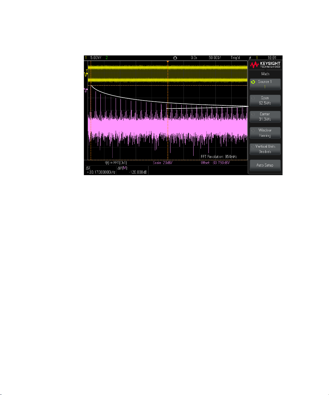
Figure 2 Aliasing
Quick Reference 2
Because the frequency span goes from ≈ 0 to the Nyquist frequency, the best way
to prevent aliasing is to make sure that the frequency span is greater than the
frequencies of significant energy present in the input signal.
FFT Spectral Leakage
The FFT operation assumes that the time record repeats. Unless there is an
integral number of cycles of the sampled waveform in the record, a discontinuity is
created at the end of the record. This is referred to as leakage. In order to minimize
spectral leakage, windows that approach zero smoothly at the beginning and end
of the signal are employed as filters to the FFT. The FFT Menu provides four
windows: Hanning, Flat Top, Rectangular, and Blackman-Harris. For more
information on leakage, see Keysight Application Note 243, The Fundamentals of
Signal Analysis at
http://literature.cdn.keysight.com/litweb/pdf/5952-8898E.pdf.
Keysight InfiniiVision 1000 X-Series Oscilloscopes User's Guide 45
Page 46

2 Quick Reference
TIP
Math Waveforms
Math functions can be performed on analog channels and lower math functions.
The resulting math waveform is displayed in light purple.
Table 8 Math Features
Feature Front Panel Key/Softkey Location (see built-in help for more information)
Math operator [Math] > Operator (Add, Subtract, Multiply, Divide, FFT Magnitude, FFT Phase, Low Pass Filter)
Cascaded math
functions
Math function
waveforms, scale
Math function
waveforms, offset
[Math] > Source
[Math] > Scale, Entry knob
[Math] > Offset, Entry knob
Math Operating Hints
Table 9 FFT (Magnitude), FFT (Phase) Operator Features
Feature Front Panel Key/Softkey Location (see built-in help for more information)
Auto setup [Math] > Auto Setup
Span/center [Math] > More > Span
If the analog channel or math function is clipped (not fully displayed on screen) the resulting
displayed math function will also be clipped.
Once the function is displayed, the analog channel(s) may be turned off for better viewing of
the math waveform.
The math function waveform can be measured using [Cursors] and/or [Meas].
[Math] > More > Center
Window function [Math] > More > Window (Hanning, Flat Top, Rectangular, Blackman Harris, see also "FFT Spectral
Leakage" on page 45)
46 Keysight InfiniiVision 1000 X-Series Oscilloscopes User's Guide
Page 47

Quick Reference 2
Table 9 FFT (Magnitude), FFT (Phase) Operator Features (continued)
Feature Front Panel Key/Softkey Location (see built-in help for more information)
Vertical units [Math] > More > Vertical Units (For FFT (Magnitude): Decibels or V RMS. For FFT (Phase): Radians or
Degrees.)
FFT (Phase) zero
phase reference point
[Math] > More > Zero Phase Ref (Trigger, Entire Display)
Table 10 Low Pass Filter Operator Features
Feature Front Panel Key/Softkey Location (see built-in help for more information)
Math low-pass filter
cutoff frequency
[Math] > Bandwidth
Units for Math Waveforms
Units for each input channel can be set to Volts or Amps using the Units softkey in
the channel's Probe Menu. Units for math function waveforms are:
Math function Units
add or subtract V or A
multiply
FFT Magnitude dB (decibels) or V RMS.
FFT Phase degrees or radians
2
, A2, or W (Volt-Amp)
V
A scale unit of U (undefined) will be displayed for math functions when two source
channels are used and they are set to dissimilar units and the combination of units
cannot be resolved.
Keysight InfiniiVision 1000 X-Series Oscilloscopes User's Guide 47
Page 48

2 Quick Reference
Reference Waveforms
Analog channel or math waveforms can be saved to one of two reference
waveform locations in the oscilloscope. Then, a reference waveform can be
displayed and compared against other waveforms. One reference waveform can
be displayed at a time.
Table 11 Reference Waveform Features
Feature Front Panel Key/Softkey Location (see built-in help for more information)
Reference waveforms,
display
Reference waveforms,
save
Reference waveforms,
skew
Reference waveforms,
scale
Reference waveforms,
offset
Reference waveforms,
clear
Reference waveforms,
info
Reference waveforms,
info, transparent
background
Reference waveforms,
save/recall from USB
storage device
[Ref] > Display Ref
[Ref] > Save/Clear > Source, [Ref] > Save/Clear > Save to
[Ref] > Skew, Entry knob
[Ref] > Scale, Entry knob
[Ref] > Offset, Entry knob
[Ref] > Save/Clear > Clear
[Save/Recall] > Default/Erase > Secure Erase
[Ref] > Save/Clear > Display Info
[Ref] > Save/Clear > Transparent
[Save/Recall] > Save > Format, Reference Waveform data (*.h5)
[Save/Recall] > Recall > Recall:, Reference Waveform data (*.h5)
48 Keysight InfiniiVision 1000 X-Series Oscilloscopes User's Guide
Page 49

Display Settings
You can adjust the intensity of displayed analog input channel waveforms to
account for various signal characteristics, such as fast time/div settings and low
trigger rates.
You can turn on waveform persistence, where the oscilloscope updates the display
with new acquisitions, but does not immediately erase the results of previous
acquisitions. All previous acquisitions are displayed with reduced intensity. New
acquisitions are shown in their normal color with normal intensity.
Table 12 Display Features
Feature Front Panel Key/Softkey Location (see built-in help for more information)
Quick Reference 2
Waveform intensity
(for analog input
channels)
Persistence, infinite
Persistence, variable [Display] > Persistence > Persistence, Variable Persistence, [Display] > Persistence > Time,
Clear persistence [Display] > Persistence > Clear Persistence
Clear display [Display] > Clear Display
Grid intensity
Grid type [Display] > Grid > Grid (Full, mV, IRE)
Waveform labels [Display] > Labels >
Label library reset [Utility] > Options > Preferences > Default Library
Annotations [Display] > Annotation >
[Intensity] (small round key just below Entry knob)
Increasing the intensity lets you see the maximum amount of noise and infrequently occurring
events. Reducing the intensity can expose more detail in complex signals.
[Display] > Persistence > Persistence, ∞Persistence
Entry knob
You can also configure the [Quick Action] key to clear the display. See "Configuring the [Quick
Action] Key" on page 90.
[Display] > Grid > Intensity, Entry knob
See also "To load a list of labels from a text file you create" on page 50.
Keysight InfiniiVision 1000 X-Series Oscilloscopes User's Guide 49
Page 50

2 Quick Reference
Table 12 Display Features (continued)
Feature Front Panel Key/Softkey Location (see built-in help for more information)
Freeze display You must configure the [Quick Action] key to freeze the display. See "Configuring the [Quick
Action] Key" on page 90.
Many activities, such as adjusting the trigger level, adjusting vertical or horizontal settings, or saving
data will un-freeze the display.
To load a list of labels from a text file you create
It may be convenient to create a list of labels using a text editor, then load the
label list into the oscilloscope. This lets you type on a keyboard rather than edit
the label list using the oscilloscope's controls.
You can create a list of up to 75 labels and load it into the oscilloscope. Labels are
added to the beginning of the list. If more than 75 labels are loaded, only the first
75 are stored.
To load labels from a text file into the oscilloscope:
1 Use a text editor to create each label. Each label can be up to ten characters in
length. Separate each label with a line feed.
2 Name the file labellist.txt and save it on a USB mass storage device such as a
thumb drive.
3 Load the list into the oscilloscope using the File Explorer (press [Utility] > File
Explorer).
50 Keysight InfiniiVision 1000 X-Series Oscilloscopes User's Guide
Page 51

Quick Reference 2
NOTE
Label List Management
When you press the Library softkey, you will see a list of the last 75 labels used. The list does
not save duplicate labels. Labels can end in any number of trailing digits. As long as the base
string is the same as an existing label in the library, the new label will not be put in the library.
For example, if label A0 is in the library and you make a new label called A12345, the new
label is not added to the library.
When you save a new user-defined label, the new label will replace the oldest label in the list.
Oldest is defined as the longest time since the label was last assigned to a channel. Any time
you assign any label to a channel, that label will move to the newest in the list. Thus, after you
use the label list for a while, your labels will predominate, making it easier to customize the
instrument display for your needs.
When you reset the label library list (see next topic), all of your custom labels will be deleted,
and the label list will be returned to its factory configuration.
Keysight InfiniiVision 1000 X-Series Oscilloscopes User's Guide 51
Page 52

2 Quick Reference
Triggers
Trigger Knobs and Keys
A trigger setup tells the oscilloscope when to acquire and display data. For
example, you can set up to trigger on the rising edge of the analog channel 1 input
signal.
You can use any input channel or the Ext Trig input BNC as the source for most
trigger types (see "External Trigger Input" on page 55).
Changes to the trigger setup are applied immediately. If the oscilloscope is
stopped when you change a trigger setup, the oscilloscope uses the new
specification when you press [Run/Stop] or [Single]. If the oscilloscope is running
when you change a trigger setup, it uses the new trigger definition when it starts
the next acquisition.
You can save trigger setups along with the oscilloscope setup (see "Save/Recall
(Setups, Screens, Data)" on page 84).
Trigger Types
In addition to the edge trigger type, you can set up triggers on pulse widths and
video signals. In the DSOX1000-Series oscilloscopes, you can also set up triggers
on patterns, rising and falling edge transition times, and setup and hold violations.
52 Keysight InfiniiVision 1000 X-Series Oscilloscopes User's Guide
Page 53

Table 13 Trigger Type Features
Feature Front Panel Key/Softkey Location (see built-in help for more information)
Trigger level Turn the trigger Level knob.
Also: [Analyze] > Features, Trigger Levels.
The edge trigger level for the Line source is not adjustable. This trigger is synchronized with the
power line supplied to the oscilloscope.
Trigger t ype
Edge trigger [Auto Scale] (sets up an Edge trigger)
Pulse width trigger [Trigger] > Trigger Type, Pulse Width
Video trigger [Trigger] > Trigger Type, Video
[Trigger] > Trigger Type (Edge, Pulse Width, Video, Serial 1, Pattern
*
)
Hold
[Trigger] > Trigger Type, Edge
NOTE: Many video signals are produced from 75
sources, a 75
input.
Ω terminator (such as a Keysight 11094B) should be connected to the oscilloscope
Ω sources. To provide correct matching to these
*
, Rise/Fall Time*, Setup and
Quick Reference 2
Pattern trigger [Trigger] > Trigger Type, Pattern
Rise/fall edge
transition time trigger
Setup and hold
violation trigger
Serial bus trigger [Trigger] > Trigger Type, Serial 1
*
Pattern, Rise/Fall Time, and Setup and Hold trigger types are available on DSOX1000-Series models only
[Trigger] > Trigger Type, Rise/Fall Time
[Trigger] > Trigger Type, Setup and Hold
See "Serial Bus Decode/Trigger" on page 78.
Trigger Mode, Coupling, Reject, Holdoff
Noisy Signals If the signal you are probing is noisy, you can set up the oscilloscope to reduce the
noise in the trigger path and on the displayed waveform. First, stabilize the
displayed waveform by removing the noise from the trigger path. Second, reduce
the noise on the displayed waveform.
1 Connect a signal to the oscilloscope and obtain a stable display.
Keysight InfiniiVision 1000 X-Series Oscilloscopes User's Guide 53
Page 54

2 Quick Reference
2 Remove the noise from the trigger path by turning on high-frequency rejection,
low-frequency rejection, or noise reject.
3 Use "Selecting the Acquisition Mode" on page 56 to reduce noise on the
displayed waveform.
Table 14 Trigger Mode, Coupling, Reject, Holdoff Features
Feature Front Panel Key/Softkey Location (see built-in help for more information)
Trigger mode [Trigger] > Mode
You can also configure the [Quick Action] key to toggle between the Auto and Normal trigger modes.
See "Configuring the [Quick Action] Key" on page 90.
Auto trigger mode [Trigger] > Mode, Auto
If the specified trigger conditions are not found, triggers are forced and acquisitions are made so that
signal activity is displayed on the oscilloscope. The Auto trigger mode is appropriate when:
• Checking DC signals or signals with unknown levels or activity.
• When trigger conditions occur often enough that forced triggers are unnecessary.
Normal trigger mode [Trigger] > Mode, Normal
Triggers and acquisitions only occur when the specified trigger conditions are found. The Normal
trigger mode is appropriate when:
• You only want to acquire specific events specified by the trigger settings.
• Making single-shot acquisitions with the [Single] key.
Often with single-shot acquisitions, you must initiate some action in the device under test, and
you do not want the oscilloscope to auto-trigger before that happens. Before initiating the action
in the circuit, wait for the trigger condition indicator Trig 'd? to flash (this tells you the pre-trigger
buffer is filled).
Force trigger [Force]
When in the Normal trigger mode and no triggers are occurring, you can force a trigger to acquire
and display waveforms (which may show why triggers are not occurring).
Trigger coupling [Trigger] > Coupling (DC, AC, LF Reject, TV/Video)
NOTE: Trigger coupling is independent of channel coupling (see "Vertical Controls" on page 38).
Trigger noise reject [Trigger] > Noise Rej
Trigger high frequency
reject
[Trigger] > HF Reject
54 Keysight InfiniiVision 1000 X-Series Oscilloscopes User's Guide
Page 55

Table 14 Trigger Mode, Coupling, Reject, Holdoff Features (continued)
CAUTION
Feature Front Panel Key/Softkey Location (see built-in help for more information)
Trigger holdoff [Trigger] > Holdoff
The correct holdoff setting is typically slightly less than one repetition of the waveform.
External Trigger Input
The external trigger input can be used as a source in several of the trigger types.
The external trigger BNC input is labeled Ext Trig.
Maximum voltage at oscilloscope external trigger input
30 Vrms
The external trigger input impedance is 1M Ohm. This lets you use passive probes
for general-purpose measurements. The higher impedance minimizes the loading
effect of the oscilloscope on the device under test.
Quick Reference 2
Table 15 External Trigger Features
Feature Front Panel Key/Softkey Location (see built-in help for more information)
External trigger units [External] > Units (Volts, Amps)
External trigger
attenuation
External trigger
threshold
External trigger range
External trigger
waveform position
[External] > Probe, Ratio/Decibels, Entry knob
[External] > Threshold, Entry knob
[External] > Range, Entry knob
For DSOX1000-Series oscilloscopes only. On EDUX1000-Series oscilloscopes, the range is fixed at
8 V when you are using a 1:1 probe.
[External] > Position, Entry knob
Keysight InfiniiVision 1000 X-Series Oscilloscopes User's Guide 55
Page 56

2 Quick Reference
Acquisition Control
This section shows how to use the oscilloscope's acquisition controls.
Selecting the Acquisition Mode
When selecting the oscilloscope acquisition mode, keep in mind that samples are
normally decimated (thrown away) at slower time/div settings.
At slower time/div settings, the effective sample rate drops (and the effective
sample period increases) because the acquisition time increases and the
oscilloscope's digitizer is sampling faster than is required to fill memory.
For example, suppose an oscilloscope's digitizer has a sample period of 1 ns
(maximum sample rate of 1 GSa/s) and a 1 M memory depth. At that rate, memory
is filled in 1 ms. If the acquisition time is 100 ms (10 ms/div), only 1 of every 100
samples is needed to fill memory.
Table 16 Acquisition Features
Feature Front Panel Key/Softkey Location (see built-in help for more information)
Acquisition mode [Acquire] > Acq Mode
Normal acquisition
mode
Peak detect
acquisition mode
Averaging acquisition
mode
High resolution
acquisition mode
[Acquire] > Acq Mode, Normal
At slower time/div settings, normal decimation occurs, and there is no averaging. Use this mode for
most waveforms.
[Acquire] > Acq Mode, Peak Detect
At slower time/div settings when decimation would normally occur, the maximum and minimum
samples in the effective sample period are stored. Use this mode for displaying narrow pulses that
occur infrequently.
[Acquire] > Acq Mode, Averaging, [Acquire] > # Avgs
At all time/div settings, the specified number of triggers are averaged together. Use this mode for
reducing noise and increasing resolution of periodic signals without bandwidth or rise time
degradation.
[Acquire] > Acq Mode, High Resolution
At slower time/div settings, all samples in the effective sample period are averaged and the average
value is stored. Use this mode for reducing random noise.
56 Keysight InfiniiVision 1000 X-Series Oscilloscopes User's Guide
Page 57

Quick Reference 2
Table 17 Segmented Memory Acquisition Features, Available on DSOX1000-Series Models Only
Feature Front Panel Key/Softkey Location (see built-in help for more information)
Segmented memory
acquisitions
Segmented memory
navigation
Segmented memory
and persistence
Segmented memory,
save to USB storage
device
Overview of Sampling
[Acquire] > Segmented > Segmented, # of Segs, [Run] or [Single]
After each segment fills, the oscilloscope re-arms and is ready to trigger in about 8 µs. Remember
though, for example: if the horizontal time per division control is set to 5 µs/div, and the Time
Reference is set to Center, it will take at least 50 µs to fill all ten divisions and re-arm. (That is 25 µs
to capture pre-trigger data and 25 µs to capture post-trigger data.)
[Acquire] > Segmented > Current Seg
[Display] > Persistence, Infinite
[Acquire] > Segmented > Analyze Segments
[Save/Recall] > Save > Format (CSV, ASCII XY, or BIN) > Settings > Save Seg (Current, All)
∞ Persistence or Variable Persistence
To understand the oscilloscope's sampling and acquisition modes, it is helpful to
understand sampling theory, aliasing, oscilloscope bandwidth and sample rate,
oscilloscope rise time, oscilloscope bandwidth required, and how memory depth
affects sample rate.
Sampling Theory
The Nyquist sampling theorem states that for a limited bandwidth (band-limited)
signal with maximum frequency f
must be greater than twice the maximum frequency f
signal be uniquely reconstructed without aliasing.
, the equally spaced sampling frequency fS
MAX
, in order to have the
MAX
f
= fS/2 = Nyquist frequency (fN) = folding frequency
MAX
Aliasing
Aliasing occurs when signals are under-sampled (fS < 2f
distortion caused by low frequencies falsely reconstructed from an insufficient
number of sample points.
Keysight InfiniiVision 1000 X-Series Oscilloscopes User's Guide 57
). Aliasing is the signal
MAX
Page 58

2 Quick Reference
Figure 3 Aliasing
Oscilloscope Bandwidth and Sample Rate
58 Keysight InfiniiVision 1000 X-Series Oscilloscopes User's Guide
An oscilloscope's bandwidth is typically described as the lowest frequency at
which input signal sine waves are attenuated by 3 dB (-30% amplitude error).
At the oscilloscope bandwidth, sampling theory says the required sample rate is f
. However, the theory assumes there are no frequency components above
= 2f
BW
(fBW in this case) and it requires a system with an ideal brick-wall frequency
f
MAX
response.
S
Page 59

Quick Reference 2
[
H
[
C
"(Y7
6iiZcjVi^dc
;gZfjZcXn
%Y7
Figure 4 Theoretical Brick-Wall Frequency Response
However, digital signals have frequency components above the fundamental
frequency (square waves are made up of sine waves at the fundamental frequency
and an infinite number of odd harmonics), and typically, for 500 MHz bandwidths
and below, oscilloscopes have a Gaussian frequency response.
Keysight InfiniiVision 1000 X-Series Oscilloscopes User's Guide 59
Page 60

2 Quick Reference
Limiting oscilloscope bandwidth (fBW) to 1/4 the sample rate (fS/4)
reduces frequency components above the Nyquist frequency (f
N).
[
H
[
C
[H$)
"(Y7
6iiZcjVi^dc
6a^VhZY[gZfjZcXn
XdbedcZcih
;gZfjZcXn
%Y7
Figure 5 Sample Rate and Oscilloscope Bandwidth
So, in practice, an oscilloscope's sample rate should be four or more times its
bandwidth: f
= 4fBW. This way, there is less aliasing, and aliased frequency
S
components have a greater amount of attenuation.
See Also Evaluating Oscilloscope Sample Rates vs. Sampling Fidelity: How to Make the
Most Accurate Digital Measurements, Keysight Application Note 1587
(http://literature.cdn.keysight.com/litweb/pdf/5989-5732EN.pdf)
Oscilloscope Rise Time
Closely related to an oscilloscope's bandwidth specification is its rise time
specification. Oscilloscopes with a Gaussian-type frequency response have an
approximate rise time of 0.35/f
An oscilloscope's rise time is not the fastest edge speed that the oscilloscope can
accurately measure. It is the fastest edge speed the oscilloscope can possibly
produce.
60 Keysight InfiniiVision 1000 X-Series Oscilloscopes User's Guide
based on a 10% to 90% criterion.
BW
Page 61

Quick Reference 2
Oscilloscope Bandwidth Required
The oscilloscope bandwidth required to accurately measure a signal is primarily
determined by the signal's rise time, not the signal's frequency. You can use these
steps to calculate the oscilloscope bandwidth required:
1 Determine the fastest edge speeds.
You can usually obtain rise time information from published specifications for
devices used in your designs.
2 Compute the maximum "practical" frequency component.
From Dr. Howard W. Johnson's book, High-Speed Digital Design – A
Handbook of Black Magic, all fast edges have an infinite spectrum of frequency
components. However, there is an inflection (or "knee") in the frequency
spectrum of fast edges where frequency components higher than f
insignificant in determining the shape of the signal.
= 0.5 / signal rise time (based on 10% - 90% thresholds)
f
knee
= 0.4 / signal rise time (based on 20% - 80% thresholds)
f
knee
3 Use a multiplication factor for the required accuracy to determine the
oscilloscope bandwidth required.
knee
are
Required accuracy Oscilloscope bandwidth required
20% fBW = 1.0 x f
10% fBW = 1.3 x f
3% fBW = 1.9 x f
knee
knee
knee
See Also Choosing an Oscilloscope with the Right Bandwidth for your Application, Keysight
Application Note 1588
(http://literature.cdn.keysight.com/litweb/pdf/5989-5733EN.pdf)
Memory Depth and Sample Rate
The number of points of oscilloscope memory is fixed, and there is a maximum
sample rate associated with oscilloscope's analog-to-digital converter; however,
the actual sample rate is determined by the time of the acquisition (which is set
according to the oscilloscope's horizontal time/div scale).
Keysight InfiniiVision 1000 X-Series Oscilloscopes User's Guide 61
Page 62

2 Quick Reference
sample rate = number of samples / time of acquisition
For example, when storing 50 µs of data in 50,000 points of memory, the actual
sample rate is 1 GSa/s.
Likewise, when storing 50 ms of data in 50,000 points of memory, the actual
sample rate is 1 MSa/s.
The actual sample rate is displayed in the right-side information area.
The oscilloscope achieves the actual sample rate by throwing away (decimating)
unneeded samples.
62 Keysight InfiniiVision 1000 X-Series Oscilloscopes User's Guide
Page 63

Cursors
X Cursors X cursors are vertical dashed lines that adjust horizontally and can be used to
Y Cursors Y cursors are horizontal dashed lines that adjust vertically and can be used to
Quick Reference 2
Cursors are horizontal and vertical markers that indicate X-axis values and Y-axis
values on a selected waveform source. You can use cursors to make custom
voltage, time, phase, or ratio measurements on oscilloscope signals.
Cursor information is displayed at the bottom of the screen.
measure time (s), frequency (1/s), phase (°), and ratio (%).
When used with the FFT math function as a source, the X cursors indicate
frequency.
In XY horizontal mode, the X cursors display channel 1 values (Volts or Amps).
measure Volts or Amps, dependent on the channel Probe Units setting, or they can
measure ratios (%). When math functions are used as a source, the measurement
units correspond to that math function.
The Y cursors adjust vertically and typically indicate values relative to the
waveform's ground point, except math FFT where the values are relative to 0 dB.
In XY horizontal mode, the Y cursors display channel 2 values (Volts or Amps).
Cursor Knobs and Keys
Cursor Softkey Controls
Keysight InfiniiVision 1000 X-Series Oscilloscopes User's Guide 63
Page 64

2 Quick Reference
Table 18 Cursor Features
Feature Front Panel Key/Softkey Location (see built-in help for more information)
Cursors mode [Cursors] > Mode
Manual cursors mode [Cursors] > Mode, Manual (and use Cursors knob to select and adjust)
Track Waveform
cursors mode
Measure cursors
mode
Binary cursors mode [Cursors] > Mode, Binary
Hex cursors mode [Cursors] > Mode, Hex
Cursors X units [Cursors] > Units > X Units (Seconds, Hz, Phase, Ratio)
Cursors Y units [Cursors] > Units > Y Units (Base, Ratio)
[Cursors] > Mode, Track Waveform
[Meas] (cursors show locations used for most recently added measurement)
64 Keysight InfiniiVision 1000 X-Series Oscilloscopes User's Guide
Page 65

Measurements
NOTE
NOTE
The [Meas] key lets you make automatic measurements on waveforms. Some
measurements can be made only on analog input channels.
If a portion of the waveform required for a measurement is not displayed or does not display
enough resolution to make the measurement (approximately 4% of full scale), the result will
be displayed as greater than a value, less than a value, not enough edges, not enough
amplitude (low signal), or waveform is clipped.
The results of the most recent measurements are displayed in the Measurements
information area at the bottom of the screen.
Cursors are turned on to show the portion of the waveform being measured for the
most recently selected measurement (right-most in the bottom measurement
area).
Post Acquisition Processing
Quick Reference 2
In addition to changing display parameters after the acquisition, you can perform all of the
measurements and math functions after the acquisition. Measurements and math functions
will be recalculated as you pan and zoom and turn channels on and off. As you zoom in and out
on a signal using the horizontal scale knob and vertical volts/division knob, you affect the
resolution of the display. Because measurements and math functions are performed on
displayed data, you affect the resolution of functions and measurements.
The units of math waveforms are described in "Units for Math Waveforms" on
page 47.
All measurements are available for analog channel waveforms. All measurements
except Counter are available for math waveforms other than FFT. A limited set of
measurements is available for math FFT waveforms. Use the cursors to make other
measurements on FFT.
Keysight InfiniiVision 1000 X-Series Oscilloscopes User's Guide 65
Page 66

2 Quick Reference
Table 19 Measurement Features
Feature Front Panel Key/Softkey Location (see built-in help for more information)
Measurement type [Meas] > Type:
Snapshot all
measurements
Voltage
measurements
Time measurements [Meas] > Type: (Period, Frequency, Counter, + Width, – Width, Bit Rate, + Duty Cycle, - Duty Cycle,
Measurement
thresholds
Measurement window [Meas] > Settings > Meas Window (Auto Select, Main, Zoom)
Clear measurements [Meas] > Clear Meas >
[Meas] > Type: Snapshot All, Add Measurement
You can also configure the [Quick Action] key to display the Snapshot All popup. See "Configuring
the [Quick Action] Key" on page 90.
[Meas] > Type: (Peak-Peak, Maximum, Minimum, Amplitude, Top, Base, Overshoot, Preshoot,
Average, DC RMS, AC RMS), Add Measurement
Rise Time, Fall Time, Delay, Phase, X at Min Y, X at Max Y), Add Measurement
The Counter measurement is available when the edge or pulse width trigger mode is selected and
the measurement source is the same as the trigger source.
[Meas] > Settings > Thresholds >
Also: [Analyze] > Features, Measurement Thresholds.
66 Keysight InfiniiVision 1000 X-Series Oscilloscopes User's Guide
Page 67

Mask Testing
Mask testing is available on the DSOX1000-Series oscilloscope models.
One way to verify a waveform's compliance to a particular set of parameters is to
use mask testing. A mask defines a region of the oscilloscope's display in which
the waveform must remain in order to comply with chosen parameters.
Compliance to the mask is verified point-by-point across the display. Mask test
operates on displayed analog channels; it does not operate on channels that are
not displayed.
Table 20 Mask Testing Features
Feature Front Panel Key/Softkey Location (see built-in help for more information)
Quick Reference 2
Mask testing
enable/disable
Mask statistics [Analyze] > Statistics >
Mask test run until [Analyze] > Setup > Run Until (Forever, Minimum # of Tests, Minimum Time, Minimum Sigma)
Mask test error action [Analyze] > Setup > On Error (Stop, Save, Print, Measure)
Mask test source lock [Analyze] > Setup > Source Lock
Auto mask creation [Analyze] > Automask >
Clear mask [Analyze] > Clear Mask
Mask files, save/recall
from USB storage
device
[Analyze] > Features, Entry knob to select Mask Test, push Entry knob to enable or disable
[Save/Recall] > Save > Format, Mask (*.msk)
[Save/Recall] > Recall > Recall:, Mask (*.msk)
Creating/Editing Mask Files
A mask file contains the following sections:
• Mask File Identifier.
•Mask Title.
• Mask Violation Regions.
• Oscilloscope Setup Information.
Mask File Identifier The Mask File Identifier is MASK_FILE_548XX.
Keysight InfiniiVision 1000 X-Series Oscilloscopes User's Guide 67
Page 68

2 Quick Reference
Mask Title The Mask Title is a string of ASCII characters. Example: autoMask CH1 OCT 03
Mask Violation
Regions
09:40:26 2008
When a mask file contains the keyword "autoMask" in the title, the edge of the
mask is passing by definition. Otherwise, the edge of the mask is defined as a
failure.
Region 1
Region 2
Up to 8 regions can be defined for a mask. They can be numbered 1-8. They can
appear in any order in the .msk file. The numbering of the regions must go from
top to bottom, left to right.
An Automask file contains two special regions: the region "glued" to the top of the
display, and the region that is "glued" to the bottom. The top region is indicated by
y-values of "MAX" for the first and last points. The bottom region is indicated by
y-values of "MIN" for the first and last points.
The top region must be the lowest numbered region in the file. The bottom region
must be the highest numbered region in the file.
Region number 1 is the top mask region. The vertices in Region 1 describe points
along a line; that line is the bottom edge of the top portion of the mask.
Similarly, the vertices in Region 2 describe the line that forms the top of the
bottom part of the mask.
68 Keysight InfiniiVision 1000 X-Series Oscilloscopes User's Guide
Page 69

Quick Reference 2
The vertices in a mask file are normalized. There are four parameters that define
how values are normalized:
•X1
• ΔX
•Y1
•Y2
These four parameters are defined in the Oscilloscope Setup portion of the mask
file.
The Y-values (normally voltage) are normalized in the file using the following
equation:
Y
= (Y - Y1)/ΔY
norm
where ΔY = Y2 - Y1
To convert the normalized Y-values in the mask file to voltage:
Oscilloscope
Setup Information
Y = (Y
norm
* ΔY) + Y1
where ΔY = Y2 - Y1
The X-values (normally time) are normalized in the file using the following
equation:
X
= (X - X1)/ΔX
norm
To convert the normalized X-values to time:
X = (X
norm
* ΔX) + X1
The keywords "setup" and "end_setup" (appearing alone on a line) define the
beginning and end of the oscilloscope setup region of the mask file. The
oscilloscope setup information contains remote programming language
commands that the oscilloscope executes when the mask file is loaded.
Any legal remote programming command can be entered in this section.
The mask scaling controls how the normalized vectors are interpreted. This in turn
controls how the mask is drawn on the display. The remote programming
commands that control mask scaling are:
:MTES:SCAL:BIND 0
:MTES:SCAL:X1 -400.000E-06
:MTES:SCAL:XDEL +800.000E-06
Keysight InfiniiVision 1000 X-Series Oscilloscopes User's Guide 69
Page 70

2 Quick Reference
:MTES:SCAL:Y1 +359.000E-03
:MTES:SCAL:Y2 +2.35900E+00
Building a Mask File
The following display shows a mask that uses all eight regions.
This mask is created by recalling the following mask file:
MASK_FILE_548XX
"All Regions"
/* Region Number */ 1
/* Number of vertices */ 4
-12.50, MAX
-10.00, 1.750
10.00, 1.750
12.50, MAX
/* Region Number */ 2
/* Number of vertices */ 5
-10.00, 1.000
-12.50, 0.500
-15.00, 0.500
-15.00, 1.500
-12.50, 1.500
/* Region Number */ 3
/* Number of vertices */ 6
-05.00, 1.000
-02.50, 0.500
70 Keysight InfiniiVision 1000 X-Series Oscilloscopes User's Guide
Page 71

02.50, 0.500
05.00, 1.000
02.50, 1.500
-02.50, 1.500
/* Region Number */ 4
/* Number of vertices */ 5
10.00, 1.000
12.50, 0.500
15.00, 0.500
15.00, 1.500
12.50, 1.500
/* Region Number */ 5
/* Number of vertices */ 5
-10.00, -1.000
-12.50, -0.500
-15.00, -0.500
-15.00, -1.500
-12.50, -1.500
/* Region Number */ 6
/* Number of vertices */ 6
-05.00, -1.000
-02.50, -0.500
02.50, -0.500
05.00, -1.000
02.50, -1.500
-02.50, -1.500
/* Region Number */ 7
/* Number of vertices */ 5
10.00, -1.000
12.50, -0.500
15.00, -0.500
15.00, -1.500
12.50, -1.500
/* Region Number */ 8
/* Number of vertices */ 4
-12.50, MIN
-10.00, -1.750
10.00, -1.750
12.50, MIN
setup
:CHANnel1:RANGe +8.00E+00
:CHANnel1:OFFSet +2.0E+00
:CHANnel1:DISPlay 1
:TIMebase:MODE MAIN
:TIMebase:REFerence CENTer
:TIMebase:RANGe +50.00E-09
:TIMebase:POSition +10.0E-09
:MTESt:SOURce CHANnel1
:MTESt:ENABle 1
:MTESt:LOCK 1
:MTESt:SCALe:X1 +10.0E-09
:MTESt:SCALe:XDELta +1.0000E-09
:MTESt:SCALe:Y1 +2.0E+00
:MTESt:SCALe:Y2 +4.00000E+00
end_setup
Quick Reference 2
Keysight InfiniiVision 1000 X-Series Oscilloscopes User's Guide 71
Page 72

2 Quick Reference
NOTE
In a mask file, all region definitions need to be separated by a blank line.
Mask regions are defined by a number of (x,y) coordinate vertices (as on an
ordinary x,y graph). A "y" value of "MAX" specifies the top of the graticule, and a
"y" value of "MIN" specifies the bottom of the graticule.
If there are more than 1000 vertices in a mask region, only the first 1000 vertices will be
processed.
The mask x,y graph is related to the oscilloscope graticule using the
:MTESt:SCALe setup commands.
The oscilloscope's graticule has a time reference location (at the left, center, or
right of the screen) and a trigger (t=0) position/delay value relative to the
reference. The graticule also has a vertical ground 0 V reference (offset relative to
the center of the screen) location.
The X1 and Y1 setup commands relate the mask region's x,y graph origin to the
oscilloscope graticule's t=0 and V=0 reference locations, and the XDELta and Y2
setup commands specify the size of the graph's x and y units.
• The X1 setup command specifies the time location of the x,y graph's x origin.
• The Y1 setup command specifies the vertical location of the x,y graph's y origin.
• The XDELta setup command specifies the amount of time associated with each
x unit.
• The Y2 setup command is the vertical location of the x,y graph's y=1 value (so
in effect, Y2 – Y1 is the YDELta value).
For example:
• With a graticule whose trigger position is 10 ns (before a center screen
reference) and whose ground reference (offset) is 2 V below the center of the
screen, to place the mask region's x,y graph's origin at center screen, you would
set X1 = 10 ns and Y1 = 2 V.
• If the XDELta parameter is set to 5 ns and Y2 is set to 4 V, a mask region whose
vertices are (-1, 1), (1, 1), (1, -1), and (-1, -1) goes from 5 ns to 15 ns and from
0V to 4V.
• If you move the mask region's x,y graph origin to the t=0 and V=0 location by
setting X1 = 0 and Y1 = 0, the same vertices define a region that goes from
-5 ns to 5 ns and from -2 V to 2 V.
72 Keysight InfiniiVision 1000 X-Series Oscilloscopes User's Guide
Page 73

Quick Reference 2
NOTE
Although a mask can have up to 8 regions, in any given vertical column, it is only possible to
define 4 regions. When there are 4 regions in a vertical column, one region must be tied to the
top (using the MAX y value) and one must be tied to the bottom (using the MIN y value).
How is mask testing done? InfiniiVision oscilloscopes start mask testing by
creating a database that is 200 x 640 for the waveform viewing area. Each location
in the array is designated as either a violation or a pass area. Each time a data
point from a waveform occurs in a violation area a failure is logged. If Test All was
selected, every active analog channel is tested against the mask database for
each acquisition. Over 2 billion failures can be logged per-channel. The number of
acquisitions tested is also logged and displayed as "# of Tests".
The mask file allows greater resolution than the 200 X 640 database. Some
quantization of data occurs to reduce the mask file data for display on-screen.
Keysight InfiniiVision 1000 X-Series Oscilloscopes User's Guide 73
Page 74

2 Quick Reference
Digital Voltmeter
The Digital Voltmeter (DVM) analysis feature provides 3-digit voltage and 5-digit
frequency measurements using any analog channel. DVM measurements are
asynchronous from the oscilloscope's acquisition system and are always
acquiring.
Table 21 Digital Voltmeter Features
Feature Front Panel Key/Softkey Location (see built-in help for more information)
Digital voltmeter
enable/disable
Digital voltmeter
mode
Auto range
enable/disable
[Analyze] > Features, Entry knob to select Digital Voltmeter, push Entry knob to enable or
disable
[Analyze] > Mode (AC RMS, DC, DC RMS, Frequency)
The Frequency mode requires the Edge or Pulse Width trigger type, and the DVM source and the
trigger source must be the same analog channel.
[Analyze] > Auto Range
Auto range can be used when the DVM input channel is not used in oscilloscope triggering.
74 Keysight InfiniiVision 1000 X-Series Oscilloscopes User's Guide
Page 75

Frequency Response Analysis
On G-suffix oscilloscope models (that have a a built-in waveform generator), the
Frequency Response Analysis (FRA) feature controls the built-in waveform
generator to sweep a sine wave across a range of frequencies while measuring the
input to and output from a device under test (DUT). At each frequency, gain (A)
and phase are measured and plotted on a frequency response Bode chart.
When the frequency response analysis completes, you can move a marker across
the chart to see the measured gain and phase values at each frequency point. You
can also adjust the chart's scale and offset settings for the gain and phase plots.
Table 22 Frequency Response Analysis Features
Feature Front Panel Key/Softkey Location (see built-in help for more information)
Quick Reference 2
Frequency Response
Analysis (FRA)
enable/disable
Channels probing DUT
input V and output V
Frequency sweep start
and stop values
Waveform generator
amplitude and
expected output load
Points [Analyze] > Setup > Points
Run the analysis [Analyze] > Run Analysis
[Analyze] > Features, Entry knob to select Frequency Response Analysis, push Entry knob to
enable or disable
[Analyze] > Setup > Sources > Input V
[Analyze] > Setup > Sources > Output V
[Analyze] > Setup > Start/Stop Freq, Entry knob
[Analyze] > Setup > Amplitude, Entry knob
[Analyze] > Setup > Output Load (50
Frequency Response Analysis automatically changes the acquisition mode during the sweep to
provide a good balance between a clean signal and high throughput at each frequency. For most
frequencies, averaging is enabled with a varying number of averages.
Ω, High-Z)
Keysight InfiniiVision 1000 X-Series Oscilloscopes User's Guide 75
Page 76

2 Quick Reference
Table 22 Frequency Response Analysis Features (continued)
Feature Front Panel Key/Softkey Location (see built-in help for more information)
Adjust scale, offset,
and frequency range
of gain or phase Bode
plots
Gain, Phase, or both
plots in chart
Autoscale gain and
phase plots
View measured gain
and phase values
Frequency response
analysis display,
transparent
background
Save data to USB
storage device
[Analyze] > Chart > Select, Entry knob (Gain, Phase, Frequency)
[Analyze] > Chart > Gain Scale/Gain Offset, Entry knob (after Gain selection)
[Analyze] > Chart > Phase Scale/Phase Offset, Entry knob (after Phase selection)
[Analyze] > Chart > Start Freq/Stop Freq, Entry knob (after Frequency selection)
[Analyze] > Chart > Trace (Gain, Phase, both)
[Analyze] > Chart > Autoscale
[Analyze] > Move Marker, Entry knob
[Analyze] > Transparent
[Save/Recall] > Save > Format, Frequency Response Analysis data (*.csv)
76 Keysight InfiniiVision 1000 X-Series Oscilloscopes User's Guide
Page 77

Waveform Generator
On G-suffix oscilloscope models, a waveform generator is built into the
oscilloscope. The waveform generator gives you an easy way to provide input
signals when testing circuitry with the oscilloscope.
Waveform generator settings can be saved and recalled with oscilloscope setups.
See "Save/Recall (Setups, Screens, Data)" on page 84.
Table 23 Waveform Generator Features
Feature Front Panel Key/Softkey Location (see built-in help for more information)
Quick Reference 2
Waveform generator
waveform type
Waveform generator
expected output load
Waveform generator
logic presets
Invert shape of
waveform
Add noise to output [Wave Gen] > Settings > Add Noise
Modulation,
enable/disable
AM modulated output [Wave Gen] > Settings > Modulation > Type, Amplitude Modulation (AM)
FM modulated output [Wave Gen] > Settings > Modulation > Type, Frequency Modulation (FM)
FSK modulated output [Wave Gen] > Settings > Modulation > Type, Frequency-Shift Keying Modulation (FSK)
Restore waveform
generator defaults
[Wave Gen] > Waveform (Sine, Square, Ramp, Pulse, DC, Noise)
[Wave Gen] > Settings > Output Load (50
[Wave Gen] > Settings > Logic Presets > (TTL, CMOS 5.0V, CMOS 3.3V, CMOS 2.5V, ECL)
[Wave Gen] > Settings > Invert Output
[Wave Gen] > Settings > Modulation > Modulation
[Wave Gen] > Settings > Default Wave Gen
Ω, High-Z)
Keysight InfiniiVision 1000 X-Series Oscilloscopes User's Guide 77
Page 78

2 Quick Reference
Serial Bus Decode/Trigger
Depending on the oscilloscope model, the following hardware-accelerated serial
decode and trigger options are available:
Serial decode and trigger type: Available on: With license:
CAN (Controller Area Network) DSOX1000-Series models AUTO
I2C (Inter-IC) All 1000 X-Series models EMBD
LIN (Local Interconnect Network) DSOX1000-Series models AUTO
SPI (Serial Peripheral Interface) DSOX1000-Series models EMBD
UART (Universal Asynchronous
Receiver/Transmitter) protocols including
RS232 (Recommended Standard 232)
To determine whether these licenses are installed on your oscilloscope, press
[Help] > About Oscilloscope.
Triggering on
Serial Data
To order serial decode licenses, go to www.keysight.com and search for the
product number (for example, DSOX1AUTO) or contact your local Keysight
Technologies representative (see www.keysight.com/find/contactus).
When triggering on a slow serial signal (for example, I2C, SPI, CAN, LIN, etc.) it
may be necessary to switch from the Auto trigger mode to the Normal trigger
mode to prevent the oscilloscope from Auto-triggering and stabilize the display.
You can select the trigger mode by pressing the [Trigger] key, then the Mode
softkey.
Also, the threshold voltage level must be set appropriately for each source
channel. The threshold level for each serial signal can be set in the Signals menu.
Press the [Bus] key, then the Signals softkey.
All 1000 X-Series models EMBD
78 Keysight InfiniiVision 1000 X-Series Oscilloscopes User's Guide
Page 79

Table 24 Serial Bus Decode/Trigger Features
Feature Front Panel Key/Softkey Location (see built-in help for more information)
Quick Reference 2
Serial bus select,
enable/disable
Serial bus mode
Serial bus trigger [Trigger] > Trigger Type, Serial 1
*
CAN, LIN, and SPI are available on DSOX1000-Series models only
[Bus] > Select, Entry knob to select Serial Bus, push Select softkey or Entry knob to enable or
disable
*
[Bus] > Mode, Entry knob (CAN
The built-in help for the Mode softkey describes the decode waveforms.
, I2C, LIN*, SPI*, UART/RS232)
CAN Decode/Trigger
On DSOX1000-Series oscilloscopes, the CAN serial decode and triggering option
can be enabled with the AUTO license.
When interpreting the decode waveforms, see the Mode softkey built-in help.
Table 25 CAN Decode/Trigger Features
Feature Front Panel Key/Softkey Location (see built-in help for more information)
CAN signal setup After selecting the Serial Bus and the CAN serial bus mode, press [Bus] > Signals > to open the CAN
Signals menu. In this menu, you can select the oscilloscope source channel probing the signal and
the appropriate threshold voltage to use when decoding/triggering the signal, as well as other signal
options.
CAN baud rate
CAN sample point
CAN signal
type/polarity
CAN counters [Bus] > Reset CAN Counters
[Bus] > Signals > Baud, Entry knob
[Bus] > Signals > Sample Point, Entry knob
[Bus] > Signals > Signal, Entry knob (Rx, Tx, CAN_H, CAN_L, Differential (L-H), Differential
(H-L))
Counters run even when the oscilloscope is stopped (not acquiring data).
When an overflow condition occurs, the counter displays OVERFLOW.
Keysight InfiniiVision 1000 X-Series Oscilloscopes User's Guide 79
Page 80

2 Quick Reference
Table 25 CAN Decode/Trigger Features (continued)
Feature Front Panel Key/Softkey Location (see built-in help for more information)
CAN trigger [Trigger] > Trigger Type, Serial 1 (CAN)
[Trigger] > Trigger on: (SOF - Start of Frame, Remote Frame ID (RTR), Data Frame ID (~RTR), Remote
or Data Frame ID, Data Frame ID and Data, Error Frame, All Errors, Acknowledge Error, Overload
Frame)
For triggers where you can specify frame ID or data values, press [Trigger] > Bits > to open the CAN
Bits menu where you can enter the values.
I2C Decode/Trigger
On all 1000 X-Series oscilloscopes, the I2C serial decode and triggering option
can be enabled with the EMBD license.
When interpreting the decode waveforms, see the Mode softkey built-in help.
Table 26 I2C Decode/Trigger Features
Feature Front Panel Key/Softkey Location (see built-in help for more information)
I2C signal setup After selecting the Serial Bus and the I2C serial bus mode, press [Bus] > Signals > to open the I2C
Signals menu. In this menu, you can select the oscilloscope source channels probing the serial clock
and serial data signals. You can also specify the appropriate threshold voltages to use when
decoding and triggering on the signals.
I2C address size [Bus] > Addr Size (7 Bit, 8 Bit)
I2C trigger [Trigger] > Trigger Type, Serial 1 (I2C)
[Trigger] > Trigger on: (Start Condition, Stop Condition, Missing Acknowledge, Address with no Ack,
Restart, EEPROM Data Read, Frame (Start: Addr7: Read: Ack: Data), Frame (Start: Addr7: Write: Ack:
Data), Frame (Start: Addr7: Read: Ack: Data: Ack: Data2), Frame (Start: Addr7: Write: Ack: Data: Ack:
Data2), 10-bit Write)
For triggers where you can specify address or data values, there are additional softkeys you can use
to enter the values.
LIN Decode/Trigger
On DSOX1000-Series oscilloscopes, the LIN serial decode and triggering option
can be enabled with the AUTO license.
80 Keysight InfiniiVision 1000 X-Series Oscilloscopes User's Guide
Page 81

Quick Reference 2
When interpreting the decode waveforms, see the Mode softkey built-in help.
Table 27 LIN Decode/Trigger Features
Feature Front Panel Key/Softkey Location (see built-in help for more information)
LIN signal setup After selecting the Serial Bus and the LIN serial bus mode, press [Bus] > Signals > to open the LIN
Signals menu. In this menu, you can select the oscilloscope source channel probing the signal and
the appropriate threshold voltage to use when decoding/triggering the signal, as well as other signal
options.
LIN baud rate
LIN sample point
LIN standard
LIN sync break
LIN show parity [Bus] > Show Parity
LIN trigger [Trigger] > Trigger Type, Serial 1 (LIN)
[Bus] > Signals > Baud > Baud, Entry knob
[Bus] > Signals > Sample Point, Entry knob
[Bus] > Signals > Standard, Entry knob (LIN 1.3, LIN 2.X)
[Bus] > Signals > Sync Break, Entry knob (>= 11, >= 12, >= 13)
[Trigger] > Trigger on: (Sync - Sync Break, ID - Frame ID, ID & Data - Frame ID and Data, Parity Error,
Checksum Error)
For triggers where you can specify frame ID or data values, there are additional softkeys you can use
to enter the values.
SPI Decode/Trigger
On DSOX1000-Series oscilloscopes, the SPI serial decode and triggering option
can be enabled with the EMBD license.
When interpreting the decode waveforms, see the Mode softkey built-in help.
Keysight InfiniiVision 1000 X-Series Oscilloscopes User's Guide 81
Page 82

2 Quick Reference
Table 28 SPI Decode/Trigger Features
Feature Front Panel Key/Softkey Location (see built-in help for more information)
SPI signal setup After selecting the Serial Bus and the SPI serial bus mode, press [Bus] > Signals > to open the SPI
Signals menu. In this menu, there are separate softkeys and submenus for specifying the Clock,
MOSI/MISO, and CS (chip select) signal oscilloscope source channels and threshold voltages.
NOTE: The 2-channel DSOX1000-Series oscilloscopes support 3-wire SPI. The MOSI and MISO
signal settings are forced to be the same; essentially, you can probe one or the other.
The Display Info softkey lets you display or hide signal setup and timing diagram information.
SPI framing
SPI word size [Bus] > Word Size
SPI bit order [Bus] > Bit Order (MSB, LSB)
SPI trigger [Trigger] > Trigger Type, Serial 1 (SPI)
[Bus] > Signals > CS > Frame by, Entry knob (~CS - Not Chip Select, CS - Chip Select, Clock
Timeout)
[Trigger] > Trigger Setup > Trigger Type (Master-Out, Slave-In (MOSI) Data)
The additional softkeys let you specify the number of data bits and the value of each bit.
UART/RS232 Decode/Trigger
On all 1000 X-Series oscilloscopes, the UART/RS232 serial decode and triggering
option can be enabled with the EMBD license.
When interpreting the decode waveforms, see the Mode softkey built-in help.
Table 29 UART/RS232 Decode/Trigger Features
Feature Front Panel Key/Softkey Location (see built-in help for more information)
UART/RS232 signal
setup
After selecting the Serial Bus and the UART/RS232 serial bus mode, press [Bus] > Signals > to open
the UART Signals menu. In this menu, you can select the oscilloscope source channels probing the
Rx and Tx signals and the appropriate threshold voltage for each.
UART/RS232 bus
configuration
UART/RS232 number
of bits
After selecting the Serial Bus and the UART/RS232 serial bus mode, press [Bus] > Bus Config > to
open the UART Bus Config menu. In this menu, you can select the oscilloscope source channels
probing the Rx and Tx signals and the appropriate threshold voltage for each.
[Bus] > Bus Config > # Bits, Entry knob (5, 6, 7, 8, 9)
82 Keysight InfiniiVision 1000 X-Series Oscilloscopes User's Guide
Page 83

Table 29 UART/RS232 Decode/Trigger Features (continued)
Feature Front Panel Key/Softkey Location (see built-in help for more information)
Quick Reference 2
UART/RS232 parity
UART/RS232 baud
rate
UART/RS232 bus
polarity
UART/RS232 bit order
UART/RS232 display
base
UART/RS232 framing
UART/RS232 counters [Bus] > Settings > Reset UART Counters
UART/RS232 trigger [Trigger] > Trigger Type, Serial 1 (CAN)
[Bus] > Bus Config > Parity, Entry knob (Even, Odd, None)
[Bus] > Bus Config > Baud Rate > Baud, Entry knob
[Bus] > Bus Config > Polarity, Entry knob (Idle low, Idle high)
[Bus] > Bus Config > Bit Order, Entry knob (LSB, MSB)
[Bus] > Settings > Base, Entry knob (Hex, Binary, ASCII)
[Bus] > Settings > Framing, Entry knob (Off, 8-bit hex value)
Counters run even when the oscilloscope is stopped (not acquiring data).
When an overflow condition occurs, the counter displays OVERFLOW.
[Trigger] > Trigger Setup > Trigger (Rx Start Bit, Rx Stop Bit, Rx Data, Rx 1:Data, Rx 0:Data, Rx
X:Data, Tx Start Bit, Tx Stop Bit, Tx Data, Tx 1:Data, Tx 0:Data, Tx X:Data, Rx or Tx Parity Error)
For triggers where you can specify data values, there are additional softkeys for specifying the data
comparison operator, the data value, the data value base (Hex or ASCII), and the Nth frame burst
count.
Keysight InfiniiVision 1000 X-Series Oscilloscopes User's Guide 83
Page 84

2 Quick Reference
Save/Recall (Setups, Screens, Data)
Oscilloscope setups, reference waveforms, and mask files can be saved to internal
oscilloscope memory or to a USB storage device and recalled later. You can also
recall default or factory default setups.
Oscilloscope screen images can be saved to a USB storage device in BMP or PNG
formats.
Acquired waveform data can be saved to a USB storage device in
comma-separated value (CSV), ASCII XY, and binary (BIN) formats.
There is also a command to securely erase all the oscilloscope's non-volatile
internal memory.
Table 30 Save/Recall Features
Feature Front Panel Key/Softkey Location (see built-in help for more information)
Save setup files,
screen images,
waveform data, mask
files
Save setup files [Save/Recall] > Save > Format, Setup (*.scp)
Save screen images [Save/Recall] > Save > Format,
[Save/Recall] > Save >
You can also configure the [Quick Action] key to save setups, screen images, or data. See
"Configuring the [Quick Action] Key" on page 90.
Press to Save
• 8-bit Bitmap image (*.bmp)
• 24-bit Bitmap image (*.bmp)
• 24-bit image (*.png)
Settings >
•Setup Info
• Invert Grat
•Palette (Color, Grayscale)
84 Keysight InfiniiVision 1000 X-Series Oscilloscopes User's Guide
Page 85

Table 30 Save/Recall Features (continued)
Feature Front Panel Key/Softkey Location (see built-in help for more information)
Save waveform data [Save/Recall] > Save > Format,
•CSV data (*.csv)
• ASCII XY data (*.csv)
• Multi Channel Waveform data (*.h5)
• Binary data (*.bin)
Settings > Length (to select number of data points to be saved, see "Length Control" on page 85)
When saving waveform data, the save times depend on the chosen format: BIN=fastest,
ASCII XY=medium, CSV=slowest.
Quick Reference 2
Quick save to USB
storage device
Recall setups, mask
files, or reference
waveforms
Recall setup files [Save/Recall] > Recall > Recall:, Setup (*.scp)
Factory default setup [Save/Recall] > Default/Erase > Factory Default
Secure erase [Save/Recall] > Default/Erase > Secure Erase
[Save to USB] (once "save to USB" settings have been configured under [Save/Recall] > Save)
[Save/Recall] > Recall > Recall:
Length Control
The Length control is available when saving data to CSV, ASCII XY, or BIN format
files. It sets the number of data points that will be output to the file. Only displayed
data points are saved.
The maximum number of data points depends on these things:
• Whether acquisitions are running. When stopped, data comes from the raw
acquisition record. When running, data comes from the smaller measurement
record.
• Whether the oscilloscope was stopped using [Stop] or [Single]. Running
acquisitions split memory to provide fast waveform update rates. Single
acquisitions use full memory.
• Whether only one channel of a pair is turned on. (Channels 1 and 2 are one
pair.) Acquisition memory is divided among the channels in a pair.
Keysight InfiniiVision 1000 X-Series Oscilloscopes User's Guide 85
Page 86

2 Quick Reference
• Whether reference waveforms are on. Displayed reference waveforms consume
acquisition memory.
• Whether segmented memory (available on DSOX1000-Series models) is on.
Acquisition memory is divided by the number of segments.
• The horizontal time/div (sweep speed) setting. At faster settings, fewer data
points appear on the display.
• When saving to a CSV format file, the maximum number of data points is
50,000.
When necessary, the Length control performs a "1 of n" decimation of the data .
For example: if the Length is set to 1000, and you are displaying a record that is
5000 data points in length, four of each five data points will be decimated,
creating an output file 1000 data points in length.
86 Keysight InfiniiVision 1000 X-Series Oscilloscopes User's Guide
Page 87

Print (Screens)
You can print the complete display, including the status line and softkeys, to a
USB printer.
To set up a USB printer:
1 Connect a USB printer to the USB host port on the front panel.
2 To open the Print Config menu:
• Press [Save/Recall] > Print.
• Select the Quick Print quick action ([Utility] > Quick Action > Action, Quick Print);
then, press Settings.
Softkeys in the Print Config menu are ghosted (not available) until a printer is
connected.
Table 31 Print Config Menu Features
Feature Front Panel Key/Softkey Location (see built-in help for more information)
Quick Reference 2
Printer selection Print to, (printer)
Print options Options,
• Setup Information
• Invert Graticule Colors
• Form Feed
• Landscape
Color or grayscale
printing
Print the current
screen
Keysight InfiniiVision 1000 X-Series Oscilloscopes User's Guide 87
Palette, (Color, Grayscale)
Press to Print
To print the current screen once the printer is configured (and Quick Print is
selected as the quick action), simply press the [Quick Action] key.
For the most up-to-date listing of printers that are compatible with the
InfiniiVision oscilloscopes, please visit
www.keysight.com/find/InfiniiVision-printers.
Page 88

2 Quick Reference
Utility Settings
This section explains oscilloscope utility functions.
Table 32 Utility Features
Feature Front Panel Key/Softkey Location (see built-in help for more information)
I/O setup [Utility] > I/O >
The oscilloscope can be accessed and/or controlled remotely using the USB device port on the rear
panel (square shaped USB port).
Connect the USB device port to a computer only when the oscilloscope is turned off or when the
oscilloscope is fully booted up and running. If you make this connection while the oscilloscope is
booting up, you will likely get a "USB device not recognized" error.
For more information, see the Programmer's Guide.
File explorer [Utility] > File Explorer >
From the internal file system, under "\User Files", you can load oscilloscope setup files (from 10
locations) or mask files (from four locations).
From a connected USB storage device, you can load setup files, mask files, license files, firmware
update (*.cab) files, label files, etc. Also, you can delete files on a connected USB storage device. See
also "USB Storage Devices" on page 89.
The rectangular USB port on the front panel is a USB Series A receptacle to which you can connect
USB mass storage devices and printers.
V/div expansion
options
Transparent
backgrounds
Screen saver [Utility] > Options > Preferences > Screen Saver >
Autoscale preferences [Utility] > Options > Preferences > Autoscale >
Undo Autoscale [Utility] > Options > Preferences > Autoscale > Undo Autoscale
Fast debug Autoscale [Utility] > Options > Preferences > Autoscale > Fast Debug
Channels to be
autoscaled
[Utility] > Options > Preferences > Expand,
• Ground
• Center
[Utility] > Options > Preferences > Transparent
[Utility] > Options > Preferences > Autoscale > Channels (All Channels, Only Displayed Channels)
88 Keysight InfiniiVision 1000 X-Series Oscilloscopes User's Guide
Page 89

Table 32 Utility Features (continued)
Feature Front Panel Key/Softkey Location (see built-in help for more information)
Quick Reference 2
Acquisition mode
during autoscale
Oscilloscope clock [Utility] > Options > Clock >
Softkey menu timeout [Utility] > Options > Menu Timeout
Gen Out signal [Utility] > Options > Auxiliary > Gen Out,
User calibration
protect
User calibration [Utility] > Service > Start User Calibration
Service task support [Utility] > Service >
User calibration status [Utility] > Service > User Calibration Status
[Utility] > Options > Preferences > Autoscale > Acq Mode (Use normal acquisition mode, Preserve
acquisition mode)
• Triggers
•Mask
•WaveGen
[Utility] > Options > Auxiliary > Cal Protect
See also the Keysight InfiniiVision 1000 X-Series Oscilloscopes Service Guide. The service guide
also tells you how to:
• Clean the oscilloscope
• Check warranty and extended services status
• Contact Keysight (www.keysight.com/find/contactus)
• Return the instrument
Hardware self test [Utility] > Service > Hardware Self Test
Front panel self test [Utility] > Service > Front Panel Self Test
About oscilloscope [Help] > About Oscilloscope
Displays: model number, serial number, bandwidth, software version, and installed licenses
User interface
language
[Help] > Language
USB Storage Devices
Use your PC to create directories on a USB storage device.
Keysight InfiniiVision 1000 X-Series Oscilloscopes User's Guide 89
Page 90

2 Quick Reference
Most USB mass storage devices are compatible with the oscilloscope. However,
certain devices may be incompatible, and may not be able to be read or written to.
USB storage devices must be formatted with the FAT or FAT32 file system format.
When the USB mass storage device is connected to the oscilloscope's USB host
port, a small four-color circle icon may be displayed briefly as the USB device is
read.
You do not need to "eject" the USB mass storage device before removing it. Simply
ensure that any file operation you've initiated is done, and remove the USB drive
from the oscilloscope's host port.
Do not connect USB devices that identify themselves as hardware type "CD"
because these devices are not compatible with the InfiniiVision X-Series
oscilloscopes.
Configuring the [Quick Action] Key
The [Quick Action] key lets you perform common, repetitive actions by pressing a
single key.
Table 33 Quick Action Features
Feature Front Panel Key/Softkey Location (see built-in help for more information)
Quick action setup [Utility] > Quick Action > Action,
•Off
• Quick Measure All
• Quick Mask Statistics Reset — see "Mask Testing" on page 67.
•Quick Print — see "Print (Screens)" on page 87.
•Quick Save — see "Save/Recall (Setups, Screens, Data)" on page 84.
• Quick Recall
• Quick Freeze Display
• Quick Trigger Mode — see "Trigger Mode, Coupling, Reject, Holdoff" on page 53.
• Quick Clear Display
Quick action perform [Quick Action]
90 Keysight InfiniiVision 1000 X-Series Oscilloscopes User's Guide
Page 91

Specifications and Characteristics
For up-to-date specifications and characteristics on the 1000 X-Series
oscilloscopes, see the data sheet at: www.keysight.com/find/1000X-Series
Quick Reference 2
Keysight InfiniiVision 1000 X-Series Oscilloscopes User's Guide 91
Page 92

2 Quick Reference
Environmental Conditions
Environment Indoor use only.
Ambient
temperature
Humidity Operating: Up to 95% RH, non-condensing to temperatures up to +40 °C
Altitude Operating: to 3,000 m
Overvoltage
Category
Pollution Degree The InfiniiVision 1000 X-Series oscilloscopes may be operated in environments
Pollution Degree
Definitions
Operating: 0 °C to +50 °C
Non-operating: -10 °C to +70 °C
decreasing linearly to 50% RH at +50 °C
Non-operating: Up to 90% RH up to +65 °C (non condensing)
Non-operating to 15,300 m
This product is intended to be powered by MAINS that comply to Overvoltage
Category II, which is typical of cord-and-plug connected equipment.
of Pollution Degree 2 (or Pollution Degree 1).
Pollution Degree 1: No pollution or only dry, non-conductive pollution occurs.
The pollution has no influence. Example: A clean room or climate controlled
office environment.
Pollution Degree 2. Normally only dry non-conductive pollution occurs.
Occasionally a temporary conductivity caused by condensation may occur.
Example: General indoor environment.
Pollution Degree 3: Conductive pollution occurs, or dry, non-conductive
pollution occurs which becomes conductive due to condensation which is
expected. Example: Sheltered outdoor environment.
Declaration of Conformity
For Declarations of Conformity for Keysight products, go to:
www.keysight.com/go/conformity
92 Keysight InfiniiVision 1000 X-Series Oscilloscopes User's Guide
Page 93

Probes and Accessories
For a list of the probes and accessories that are compatible with the 1000 X-Series
oscilloscopes, see the data sheet at: www.keysight.com/find/1000X-Series
Because the 1000 X-Series oscilloscopes do not have a ring around the BNC
connector for identifying probes, you must set the probe attenuation factor
manually. See "Setting Analog Channel Probe Options" on page 40.
See Also For more information on probes and accessories, see www.keysight.com for:
• Probes and Accessories Selection Guide (5989-6162EN)
• InfiniiVision Oscilloscope Probes and Accessories Selection Guide Data Sheet
(5968-8153EN)
• For compatibility information, manuals, application notes, data sheets,
selection guides, SPICE models, and more for oscilloscope probes, see the
Probe Resource Center at: www.keysight.com/find/PRC
Quick Reference 2
Keysight InfiniiVision 1000 X-Series Oscilloscopes User's Guide 93
Page 94

2 Quick Reference
Software and Firmware Updates
From time to time Keysight Technologies releases software and firmware updates
for its products. To search for firmware updates for your oscilloscope, direct your
web browser to www.keysight.com/find/1000X-Series-sw.
To view the currently installed software and firmware press [Help] > About
Oscilloscope.
Once you have downloaded a firmware update file, you can place it on a USB
storage device and load the file using File Explorer (see "Utility Settings" on
page 88).
94 Keysight InfiniiVision 1000 X-Series Oscilloscopes User's Guide
Page 95

Acknowledgements
Table 34 Third Party Software
Quick Reference 2
Software Description and Copyright License
7-zip Copyright (C) 1999-2016 Igor Pavlov. GNU LGPL + unRAR
Boost Libraries Copyright © 2008 Beman Dawes, Rene Rivera Boost Software License
HDF5 HDF5 was developed by The HDF Group and by the National Center
for Supercomputing Applications at the University of Illinois at
Urbana-Champaign.
Copyright 2006-2016 by The HDF Group.
Copyright 1998-2006 by the Board of Trustees of the University of
Illinois.
libmspack Copyright: © 2003-2013 Stuart Caie
Source code can be obtained from the third party or by contacting
Keysight. Keysight will charge for the cost of physically performing the
source distribution.
libpng Copyright (c) 1998-2002,2004,2006-2016 Glenn Randers-Pehrson
(Version 0.96 Copyright (c) 1996, 1997 Andreas Dilger)
(Version 0.88 Copyright (c) 1995, 1996 Guy Eric Schalnat, Group 42,
Inc.)
OpenNETCF Smart
Device Framework
Copyright (c) 2001-2014 Tacke Consulting, LLC MIT License
1
restriction
(BSL-1.0)
BSD-style open source
Lesser or Library
General Public License
version 3.0 (LGPLv3)
libpng specific
TCLAP Copyright (c) 2003 Michael E. Smoot MIT License
time_ce Copyright (C) 2002 Michael Ringgaard. All rights reserved. MIT License
U-Boot (C) Copyright 2000 - 2013 Wolfgang Denk, DENX Software
Engineering, wd@denx.de.
Source code can be obtained from the third party or by contacting
Keysight. Keysight will charge for the cost of physically performing the
source distribution.
GNU General Public
License (GPL or GPLv2)
Keysight InfiniiVision 1000 X-Series Oscilloscopes User's Guide 95
Page 96

2 Quick Reference
Table 34 Third Party Software (continued)
Software Description and Copyright License
WCELIBCEX File copyright is held by a file author.
Files created for the first version of the WCELIBCEX project are
copyrighted by (c) 2006 Taxus SI Ltd., http://www.taxussi.com.pl
See comment in header of source files for more details.
zlib Copyright (C) 1995-2013 Jean-loup Gailly and Mark Adler zlib license
1
These licenses are located on the Keysight InfiniiVision oscilloscopes manuals website at
www.keysight.com/find/1000X-Series-manual.
MIT License
1
96 Keysight InfiniiVision 1000 X-Series Oscilloscopes User's Guide
Page 97

Product Markings and Regulatory Information
267459
MSIP-REM-Kst-
1A15150
These symbols are used on the 1000 X-Series oscilloscopes.
Symbol Description
Caution, risk of electric shock
Caution, refer to accompanying documentation
This symbol indicates separate collection for electrical and electronic
equipment mandated under EU law as of August 13, 2005. All electric and
electronic equipment are required to be separated from normal waste for
disposal (Reference WEEE Directive 2002/96/EC).
Indicates the time period during which no hazardous or toxic substance
elements are expected to leak or deteriorate during normal use. Forty
years is the expected useful life of the product.
The RCM mark is a registered trademark of the Australian
Communications and Media Authority.
Quick Reference 2
The CE mark is a registered trademark of the European Community.
ccr.keysight@keysight.com
ICES / NMB-001 Cet appareil ISM est conforme a la norme NMB du
Canada. This is a marking to indicate product compliance with the
Industry Canadian Interference-Causing Equipment Standard (ICES-001).
This is also a symbol of an Industrial Scientific and Medical Group 1 Class
A product (CISPR 11, Clause 4).
The CSA mark is a registered trademark of the CSA International.
South Korean Certification (KC) mark; includes the marking's identifier
code which follows this format:
MSIP-REM-YYY-ZZZZZZZZZZZZZZ.
Keysight InfiniiVision 1000 X-Series Oscilloscopes User's Guide 97
Page 98

2 Quick Reference
98 Keysight InfiniiVision 1000 X-Series Oscilloscopes User's Guide
Page 99

Index
Symbols
(-) Width measurement, 66
(+) Width measurement, 66
Numerics
10-bit write trigger, I2C, 80
A
About Oscilloscope, 89
AC channel coupling, 39
AC RMS measurement, 66
accessories, 14, 93
acquire, 56
Acquire key, 23, 35, 36
Acquisition controls, 23
acquisition memory, saving, 85
acquisition mode, 56
acquisition mode during autoscale, 89
acquisition mode, preserve during
AutoScale, 89
acquisition modes, 56
actual sample rate, 61
addition math function, 46
address size, I2C, 80
address with no ack condition, I2C
trigger, 80
aliasing, 57
aliasing, FFT, 44
altitude (environmental conditions), 92
AM (amplitude modulation), waveform
generator output, 77
Amp units, 40, 55
Amplitude measurement, 66
amplitude modulation (AM), waveform
generator output, 77
analog bus display, 41
analog channel, probe attenuation, 40
analog channel, setup, 38
analog filters, adjusting, 42
Analyze key, 24
Analyze Segments, 57
annotation, adding, 49
ASCII file format, 85
attenuation, probe, 40
attenuation, probe, external trigger, 55
auto mask creation, 67
auto range, digital voltmeter, 74
Auto Scale key, 23
Auto Setup, FFT, 42
Auto Setup, FFT (Magnitude), FFT
(Phase), 46
Auto trigger mode, 54
automatic measurements, 65
Autoscale, 19
Autoscale preferences, 88
Autoscale, undo, 19,
Average measurement, 66
averaging acquisition mode, 56
88
B
Back key, 22
bandwidth, 89
bandwidth limit, 39
bandwidth required, oscilloscope, 61
bandwidth, oscilloscope, 58
Base measurement, 66
base, UART/RS232, 83
baud rate, CAN, 79
baud rate, LIN, 81
baud rate, UART/RS232, 83
BIN file format, 85
bit order, SPI, 82
bit order, UART/RS232, 83
Bit Rate measurement, 66
Blackman Harris FFT window, 42, 46
blanking, 36
BMP file format, 84
Bode plot, frequency response
analysis, 76
brick-wall frequency response, 58
brightness of waveforms, 22
built-in help, 31
bus configuration, UART/RS232, 82
Bus key, 25, 41, 78
buttons (keys), front panel, 22
C
calibration, 89
calibration protect button, 28
CAN baud rate, 79
CAN bus trigger, 80
CAN counters, 79
CAN polarity, 79
CAN sample point, 79
CAN serial bus decode/trigger, 79
CAN signal setup, 79
cascaded math functions, 46
Center, FFT, 42
Center, FFT (Magnitude), FFT
(Phase), 46
channel labels, 49
channel, analog, 38
channel, bandwidth limit, 39
channel, coupling, 39
channel, invert, 39
channel, on/off keys, 26
channel, probe units, 40
channel, skew, 40
channel, vernier, 26
channels to be autoscaled, 88
characteristics, 91
choosing values, 23
clear display, 49
clear display, Quick Clear Display, 90
Clear measurements, 66
clear persistence, 49
clear, mask test, 67
clock, oscilloscope, 89
color printing, 87
color screen image, 84
compensate passive probes, 20, 26
Keysight InfiniiVision 1000 X-Series Oscilloscopes User's Guide 99
Page 100

Index
Conformity, Declaration of, 92
connectors, rear panel, 28
control, remote, 88
controls, front panel, 22
copyright, 2
Counter measurement, 66
counters, CAN, 79
counters, UART/RS232, 83
coupling, channel, 39
coupling, trigger, 54
crosstalk between input channels,
minimizing, 38
crosstalk problems, 42
CSV file format, 85
cursor measurements, 63
cursor units, 64
Cursors key, 24
Cursors knob, 24
cursors, binary, 64
cursors, hex, 64
cursors, manual, 64
cursors, track waveform, 64
cutoff frequency, low-pass filter, 47
D
damage, shipping, 14
data sheet, 91
date, 89
DC channel coupling, 39
DC RMS measurement, 66
DC signals, checking, 54
DC waveform generator output, 77
decibels, FFT (Magnitude) vertical
units, 47
decibels, FFT vertical units, 42
decimating samples, 62
Declaration of Conformity, 92
decode, CAN serial bus, 79
decode, I2C serial bus, 80
decode, LIN serial bus, 80
decode, SPI serial bus, 81
decode, UART/RS232 serial bus, 82
default configuration, 18
default label library, 49
default setup, 18
Default Setup key, 23
defaults, waveform generator, 77
degrees, FFT (Phase) vertical units, 47
Delay measurement, 66
delay time, 36
delete file, 88
Demo terminal, 26
digital voltmeter (DVM), 74
digital voltmeter mode, 74
Display key, 24
display multiple acquisitions, 34
display, area, 29
display, interpreting, 29
display, persistence, 49
display, softkey labels, 30
display, status line, 29
displayed channels AutoScale, 88
distortion problems, 42
Divide math function, 46
Duty cycle - measurement, 66
Duty cycle + measurement, 66
DVM (digital voltmeter), 74
E
edge speeds, 61
edge triggering, 53
EEPROM data read, I2C trigger, 80
entire display, FFT (Phase) zero phase
reference, 47
Entry knob, 23
Entry knob, push to select, 23
environmental conditions, 92
erase, secure, 85
error action, mask test, 67
expand about, 26, 88
expand about center, 88
expand about ground, 88
exporting waveform, 84
Ext Trig as Z-axis input, 36
Ext Trig input connector, 25
External key, 25
external memory device, 27
external trigger, 55
external trigger waveform, position, 55
external trigger, input impedance, 55
external trigger, probe attenuation, 55
external trigger, probe units, 55
external trigger, range, 55
external trigger, threshold, 55
F
factory default settings, 85
Fall time measurement, 66
fast debug AutoScale, 88
FAT file system format, 90
FAT32 file system format, 90
FFT (Magnitude), FFT (Phase) vertical
units, 47
FFT aliasing, 44
FFT DC value, 44
FFT key, 25
FFT magnitude math function, 46
FFT measurement hints, 42
FFT phase math function, 46
FFT resolution, 43
FFT spectral analysis, 42
FFT spectral leakage, 45
FFT vertical units, 42
FFT window, 42
file explorer, 88
file format, ASCII, 85
file format, BIN, 85
file format, BMP, 84
file format, CSV, 85
file format, PNG, 84
file, save, recall, load, 88
filter, low pass, 46
fine adjustment, vertical scale, 39
firmware updates, 94
flash drive, 27
Flat top FFT window, 42, 46
FM (frequency modulation), waveform
generator output, 77
folding frequency, 57
Force key, 25
forcing a trigger, 54
FRA (frequency response analysis), 75
frame trigger, I2C, 80
framing, SPI, 82
framing, UART/RS232, 83
freeze display, 50, 90
freeze display, Quick Freeze
Display, 90
Frequency measurement, 66
frequency modulation (FM), waveform
generator output, 77
frequency requirements, power
source, 15
100 Keysight InfiniiVision 1000 X-Series Oscilloscopes User's Guide
 Loading...