


Measurement Guide
HP ESA Spectrum Analyzers
HP Part Number E4401-90052
Printed in: USA
April 1999
© Copyright Hewlett-Packard Company 1999

Notice
The information contained in this document is subject to change
without notice.
Hewlett-Packard makes no warranty of any kind with regard to this
material, including but not limited to, the implied warranties of
merchantability and fitness for a particular purpose. Hewlett-Packard
shall not be liable for errors contained herein or for incidental or
consequential damages in connection with the furnishing, performance,
or use of this material.
Safety Notice
The following safety notes are used throughout this manual.
Familiarize yourself with the notes and their meaning before operating
this instrument.
CAUTION Caution denotes a hazard. It calls attention to a procedure that, if not
correctly performed or adhered to, would result in damage to or
destruction of the instrument. Do not proceed beyond a caution until
the indicated conditions are fully understood and met.
WARNING Warning denotes a hazard. It calls attention to a procedure
which, if not correctly performed or adhered to, could result in
injury or loss of life. Do not proceed beyond a warning note
until the indicated conditions are fully understood and met.
WARNING This is a Safety Class 1 Product (provided with a protective
earthing ground incorporated in the power cord). The mains
plug shall only be inserted in a socket outlet provided with a
protective earth contact. Any interruption of the protective
conductor inside or outside of the product is likely to make the
product dangerous. Intentional interruption is prohibited.
ii

Where to Find the Latest Information
Documentation is updatedperiodically. For thelatestinformationabout
HP ESA Spectrum Analyzers, including firmware upgrades and
application information, please visit the following Internet URL:
http://www.hp.com/go/esa.
iii

iv

Contents
1. Instrument Overview
Front-Panel Features . . . . . . . . . . . . . . . . . . . . . . . . . . . . . . . . . . . . . . . . . . . . . . . . . . . . . . . .1-2
Rear-Panel Features . . . . . . . . . . . . . . . . . . . . . . . . . . . . . . . . . . . . . . . . . . . . . . . . . . . . . . . . .1-7
Display Annotation . . . . . . . . . . . . . . . . . . . . . . . . . . . . . . . . . . . . . . . . . . . . . . . . . . . . . . . . .1-11
2.Making Basic Measurements
What is in This Chapter . . . . . . . . . . . . . . . . . . . . . . . . . . . . . . . . . . . . . . . . . . . . . . . . . . . . . .2-2
Comparing Signals . . . . . . . . . . . . . . . . . . . . . . . . . . . . . . . . . . . . . . . . . . . . . . . . . . . . . . . . . .2-3
Example 1: . . . . . . . . . . . . . . . . . . . . . . . . . . . . . . . . . . . . . . . . . . . . . . . . . . . . . . . . . . . . . . .2-3
Example 2: . . . . . . . . . . . . . . . . . . . . . . . . . . . . . . . . . . . . . . . . . . . . . . . . . . . . . . . . . . . . . . .2-5
Resolving Signals of Equal Amplitude . . . . . . . . . . . . . . . . . . . . . . . . . . . . . . . . . . . . . . . . . .2-7
Example: . . . . . . . . . . . . . . . . . . . . . . . . . . . . . . . . . . . . . . . . . . . . . . . . . . . . . . . . . . . . . . . . .2-8
Resolving Small Signals Hidden by Large Signals . . . . . . . . . . . . . . . . . . . . . . . . . . . . . . .2-10
Example: . . . . . . . . . . . . . . . . . . . . . . . . . . . . . . . . . . . . . . . . . . . . . . . . . . . . . . . . . . . . . . . .2-11
Making Better Frequency Measurements . . . . . . . . . . . . . . . . . . . . . . . . . . . . . . . . . . . . . . .2-13
Example: . . . . . . . . . . . . . . . . . . . . . . . . . . . . . . . . . . . . . . . . . . . . . . . . . . . . . . . . . . . . . . . .2-13
Decreasing the Frequency Span Around the Signal . . . . . . . . . . . . . . . . . . . . . . . . . . . . . .2-15
Example: . . . . . . . . . . . . . . . . . . . . . . . . . . . . . . . . . . . . . . . . . . . . . . . . . . . . . . . . . . . . . . . .2-15
Tracking Drifting Signals . . . . . . . . . . . . . . . . . . . . . . . . . . . . . . . . . . . . . . . . . . . . . . . . . . .2-17
Example 1: . . . . . . . . . . . . . . . . . . . . . . . . . . . . . . . . . . . . . . . . . . . . . . . . . . . . . . . . . . . . . .2-17
Example 2: . . . . . . . . . . . . . . . . . . . . . . . . . . . . . . . . . . . . . . . . . . . . . . . . . . . . . . . . . . . . . .2-19
Measuring Low Level Signals . . . . . . . . . . . . . . . . . . . . . . . . . . . . . . . . . . . . . . . . . . . . . . . . .2-21
Example 1: . . . . . . . . . . . . . . . . . . . . . . . . . . . . . . . . . . . . . . . . . . . . . . . . . . . . . . . . . . . . . .2-21
Example 2: . . . . . . . . . . . . . . . . . . . . . . . . . . . . . . . . . . . . . . . . . . . . . . . . . . . . . . . . . . . . . .2-24
Example 3: . . . . . . . . . . . . . . . . . . . . . . . . . . . . . . . . . . . . . . . . . . . . . . . . . . . . . . . . . . . . . .2-25
Example 4: . . . . . . . . . . . . . . . . . . . . . . . . . . . . . . . . . . . . . . . . . . . . . . . . . . . . . . . . . . . . . .2-27
Identifying Distortion Products . . . . . . . . . . . . . . . . . . . . . . . . . . . . . . . . . . . . . . . . . . . . . . .2-29
Distortion from the Analyzer . . . . . . . . . . . . . . . . . . . . . . . . . . . . . . . . . . . . . . . . . . . . . . .2-29
Example: . . . . . . . . . . . . . . . . . . . . . . . . . . . . . . . . . . . . . . . . . . . . . . . . . . . . . . . . . . . . . 2-29
Third-Order Intermodulation Distortion . . . . . . . . . . . . . . . . . . . . . . . . . . . . . . . . . . . . . .2-32
Example: . . . . . . . . . . . . . . . . . . . . . . . . . . . . . . . . . . . . . . . . . . . . . . . . . . . . . . . . . . . . . 2-32
Measuring Signal-to-Noise . . . . . . . . . . . . . . . . . . . . . . . . . . . . . . . . . . . . . . . . . . . . . . . . . .2-35
Making Noise Measurements . . . . . . . . . . . . . . . . . . . . . . . . . . . . . . . . . . . . . . . . . . . . . . . . .2-37
Example 1: . . . . . . . . . . . . . . . . . . . . . . . . . . . . . . . . . . . . . . . . . . . . . . . . . . . . . . . . . . . . . .2-37
Example 2: . . . . . . . . . . . . . . . . . . . . . . . . . . . . . . . . . . . . . . . . . . . . . . . . . . . . . . . . . . . . . .2-39
Example 3: . . . . . . . . . . . . . . . . . . . . . . . . . . . . . . . . . . . . . . . . . . . . . . . . . . . . . . . . . . . . . .2-40
Example 4: . . . . . . . . . . . . . . . . . . . . . . . . . . . . . . . . . . . . . . . . . . . . . . . . . . . . . . . . . . . . . .2-42
Demodulating AM Signals (Using the Analyzer As a Fixed Tuned Receiver) . . . . . . . . . .2-44
Example: . . . . . . . . . . . . . . . . . . . . . . . . . . . . . . . . . . . . . . . . . . . . . . . . . . . . . . . . . . . . . . . .2-44
Demodulating FM Signals
(Without Option BAA) . . . . . . . . . . . . . . . . . . . . . . . . . . . . . . . . . . . . . . . . . . . . . . . . . . . . . .2-47
Example: . . . . . . . . . . . . . . . . . . . . . . . . . . . . . . . . . . . . . . . . . . . . . . . . . . . . . . . . . . . . . . . .2-47
Demodulate the FM Signal. . . . . . . . . . . . . . . . . . . . . . . . . . . . . . . . . . . . . . . . . . . . . . . 2-49
3. Making Measurements
What’s in This Chapter . . . . . . . . . . . . . . . . . . . . . . . . . . . . . . . . . . . . . . . . . . . . . . . . . . . . . .3-2
Making Stimulus Response Measurements . . . . . . . . . . . . . . . . . . . . . . . . . . . . . . . . . . . . . . .3-3
What Are Stimulus Response Measurements? . . . . . . . . . . . . . . . . . . . . . . . . . . . . . . . . . .3-3
v

Contents
Using An Analyzer With A Tracking Generator . . . . . . . . . . . . . . . . . . . . . . . . . . . . . . . . .3-3
Stepping Through a Transmission Measurement . . . . . . . . . . . . . . . . . . . . . . . . . . . . . . . .3-4
Tracking Generator Unleveled Condition . . . . . . . . . . . . . . . . . . . . . . . . . . . . . . . . . . . . . .3-8
Measuring Device Bandwidth . . . . . . . . . . . . . . . . . . . . . . . . . . . . . . . . . . . . . . . . . . . . . . .3-9
Example: . . . . . . . . . . . . . . . . . . . . . . . . . . . . . . . . . . . . . . . . . . . . . . . . . . . . . . . . . . . . . 3-10
Making a Reflection Calibration Measurement . . . . . . . . . . . . . . . . . . . . . . . . . . . . . . . . . .3-12
Example: . . . . . . . . . . . . . . . . . . . . . . . . . . . . . . . . . . . . . . . . . . . . . . . . . . . . . . . . . . . . . . . .3-13
Reflection Calibration . . . . . . . . . . . . . . . . . . . . . . . . . . . . . . . . . . . . . . . . . . . . . . . . . . . . .3-13
Measuring the Return Loss . . . . . . . . . . . . . . . . . . . . . . . . . . . . . . . . . . . . . . . . . . . . . . . .3-14
Demodulating and Listening to an AM Signal . . . . . . . . . . . . . . . . . . . . . . . . . . . . . . . . . . .3-15
Example 1: . . . . . . . . . . . . . . . . . . . . . . . . . . . . . . . . . . . . . . . . . . . . . . . . . . . . . . . . . . . . . .3-15
Example 2: . . . . . . . . . . . . . . . . . . . . . . . . . . . . . . . . . . . . . . . . . . . . . . . . . . . . . . . . . . . . . .3-17
Measuring Harmonics and Harmonic Distortion . . . . . . . . . . . . . . . . . . . . . . . . . . . . . . . . .3-19
Example: . . . . . . . . . . . . . . . . . . . . . . . . . . . . . . . . . . . . . . . . . . . . . . . . . . . . . . . . . . . . . . . .3-20
Measurement Setup . . . . . . . . . . . . . . . . . . . . . . . . . . . . . . . . . . . . . . . . . . . . . . . . . . . . 3-22
Measurement Control . . . . . . . . . . . . . . . . . . . . . . . . . . . . . . . . . . . . . . . . . . . . . . . . . . . 3-24
End of Measurement. . . . . . . . . . . . . . . . . . . . . . . . . . . . . . . . . . . . . . . . . . . . . . . . . . . . 3-24
vi

1 Instrument Overview
• Front Panel
• Rear Panel
• Screen Annotation
1-1

Instrument Overview
Front-Panel Features
Front-Panel Features
Figure 1-1 Front-Panel Feature Overview
1 Viewing Angle keys allow you to adjust the display so
that it can be optimally viewed from different angles.
2 Esc. The Esc (escape) key cancels any entry in progress.
Esc will abort a print (if one is in progress) and clear
error messages from the status line at the bottom of the
display. It also clears input and tracking generator
overload conditions.
3 Menu keys are the unlabeled keys next to the screen.
The menu key labels are the annotation on the screen
next to the unlabeled keys. Most of the labeled keys on
the analyzer front panel (also called front-panel keys)
access menus of keys having related functions.
1-2 Chapter1

Instrument Overview
Front-Panel Features
4 FREQUENCY Channel, SPAN X Scale, and AMPLITUDE Y
Scale are the three large keys that activate the primary
analyzer functions and access menus of related
functions.The secondary labels on these keys (Channel,
X Scale, and Y Scale) are used in some measurements.
5 CONTROL functions access menus that allow you to
adjust the resolution bandwidth, adjust the sweep time,
and control the instrument display. They also set other
analyzer parameters needed for making
measurements.
6 MEASURE accesses a menu of keys that automate some
common analyzer measurements. Once a measurement
is running,
for defining your measurement.
Restart access additional measurement control
Meas Setup accesses additional menu keys
Meas Control and
functions.
7 SYSTEM functions affect the state of the entire
spectrum analyzer. Various setup and alignment
routines are accessed with the
System key.
The green
Preset key resets the analyzer to a known
state.
The File key menu allows you to save and load traces,
states, limit-line tables, and amplitude correction
factors to or from analyzer memory or the floppy disk
drive. The
function defined under
Save key immediately executes the Save
File in the Front-Panel Key
Reference chapter.
The Print Setup menu keys allow you to configure
hardcopy outputs. The
Print key immediately sends
hardcopy data to the printer. See the user’s guide for
more details.
8 MARKER functions control the markers, read out
frequencies and amplitudes along the analyzer trace,
automatically locate the signals of highest amplitude,
and access functions like
9 The Media Door on the right side of the front panel
Marker Noise and Band Power.
accesses the 3.5 inch disk drive and the Earphone
connector. The earphone connector provides a
connection for an earphone jack which bypasses the
internal speaker.
Chapter 1 1-3

Instrument Overview
Front-Panel Features
10 The Data Control Keys, which include the step keys,
knob, and numeric keypad, allow you to change the
numeric value of an active function.
Data control keys are used to change values for
functions such as center frequency, start frequency,
resolution bandwidth, and marker position.
The data controls will change the active function in a
manner prescribed by that function. For example, you
can change center frequency in fine steps with the
knob, in discrete steps with the step keys, or to an exact
value with the numeric keypad.
The Knob allows continuous change of functions such
as center frequency, reference level, and marker
position. It also changes the values of many functions
that change in increments only. Clockwise rotation of
the knob increases values. For continuous changes, the
extent of alteration is determined by the size of the
measurement range; the speed at which the knob is
turned affects the rate at which the values are changed.
Among other things, the knob enables you to change
the center frequency, start or stop frequency, or
reference level. For slow sweeps, the analyzer uses a
smooth panning feature which is designed to move the
trace display to the latest function value as the knob is
turned. When either center frequency or reference level
is adjusted, the signal will shift right or left or up or
down with the rotation of the knob before a new sweep
is actually taken. An asterisk is placed in the message
block (the upper right-hand corner of the analyzer
display) to indicate that the data on the screen does not
reflect data at the current setting.
The Numeric Keypad allows entry of exact values for
many of the analyzer functions. You may include a
decimal point in the number portion. If not, the decimal
point is placed at the end of the number.
Numeric entries must be terminated with a units key.
When a numeric entry is begun, the menu keys show
the units key labels. The units keys change depending
on what the active function is. For example, the units
keys for frequency span are
whereas the units for reference level are
mV, and µV.
GHz, MHz, kHz, and Hz,
+dBm, −dBm,
1-4 Chapter1

Instrument Overview
Front-Panel Features
NOTE If an entry from the numeric keypad does not coincide with an allowed
function value (for example, that of a 12 MHz bandwidth), the analyzer
defaults to the nearest allowable value.
The Step Keys (⇓⇑) allow discrete increases or
decreases of the active function value. The step size
depends upon the analyzer measurement range or on a
preset amount. Each press results in a single step
change. For those parameters with fixed values, the
next value in a sequence is selected each time a step
key is pressed. Changes are predictable and can be set
for some functions. Out-of-range values or
out-of-sequence values will not occur using these keys.
11 VOLUME. The VOLUME knob adjusts the volume of the
internal speaker. The speaker is turned on and off with
the
Speaker On Off key in the Det/Demod menu.
12 EXT KEYBOARD. The EXT KEYBOARD connector is a
6-pin mini-DIN connector for future use with PC
keyboards. It is not currently supported.
13 PROBE POWER provides power for high-impedance ac
probes or other accessories.
14 Return. The Return key accesses the previously selected
menu. Continuing to press
Return accesses earlier
menus.
15 AMPTD REF OUT provides an amplitude reference signal
of 50 MHz at –20 dBm. HP E4402B, HP E4403B,
HP E4404B, HP E4405B, HP E4407B, and
HP E4408B only.
16 Tab Keys are used to move around in the Limit editor
and the Correction editor,and to move within the fields
of the dialog box accessed by the
17 INPUT 50Ω (INPUT 75Ω for Option 1DP) is the signal
File menu keys.
input for the analyzer.
18 The Next Window key can be used to select the active
window in functions which support split-screen display
modes, such as Zone markers. In such modes, pressing
Zoom allows you to switch between the split-screen and
full-sized display of the active window.
19 Help. Press the Help key and then any front-panel or
menu key to get a short description of the key function
and the associated SCPI command. The next key you
press will remove the help window from the display.
Chapter 1 1-5

Instrument Overview
Front-Panel Features
20 RF OUT 50Ω (for Option 1DN) or RF OUT 75Ω (for
Option 1DQ) is the source output for the built-in
tracking generator. Option 1DN or 1DQ only.
CAUTION If the tracking generator output power is too high, it may damage the
device under test. Do not exceed the maximum power that the device
under test can tolerate.
21 The ❙ (On) key turns the analyzer on, while the O
(Standby) key turns most of the analyzer off. An
instrument alignment is performed (if
Auto Align is on)
every time the analyzer is turned on. After turning on
the analyzer, allow 5 minutes of warm-up time to
ensure the analyzer will meet all specifications.
NOTE The instrument continues to draw power even if the line power switch
is in standby. The detachable power cord is the instrument
disconnecting device. It disconnects the mains circuits from the mains
supply before other parts of the instrument. The front-panel switch is
only a standby switch and is not a LINE switch (disconnecting device).
1-6 Chapter1
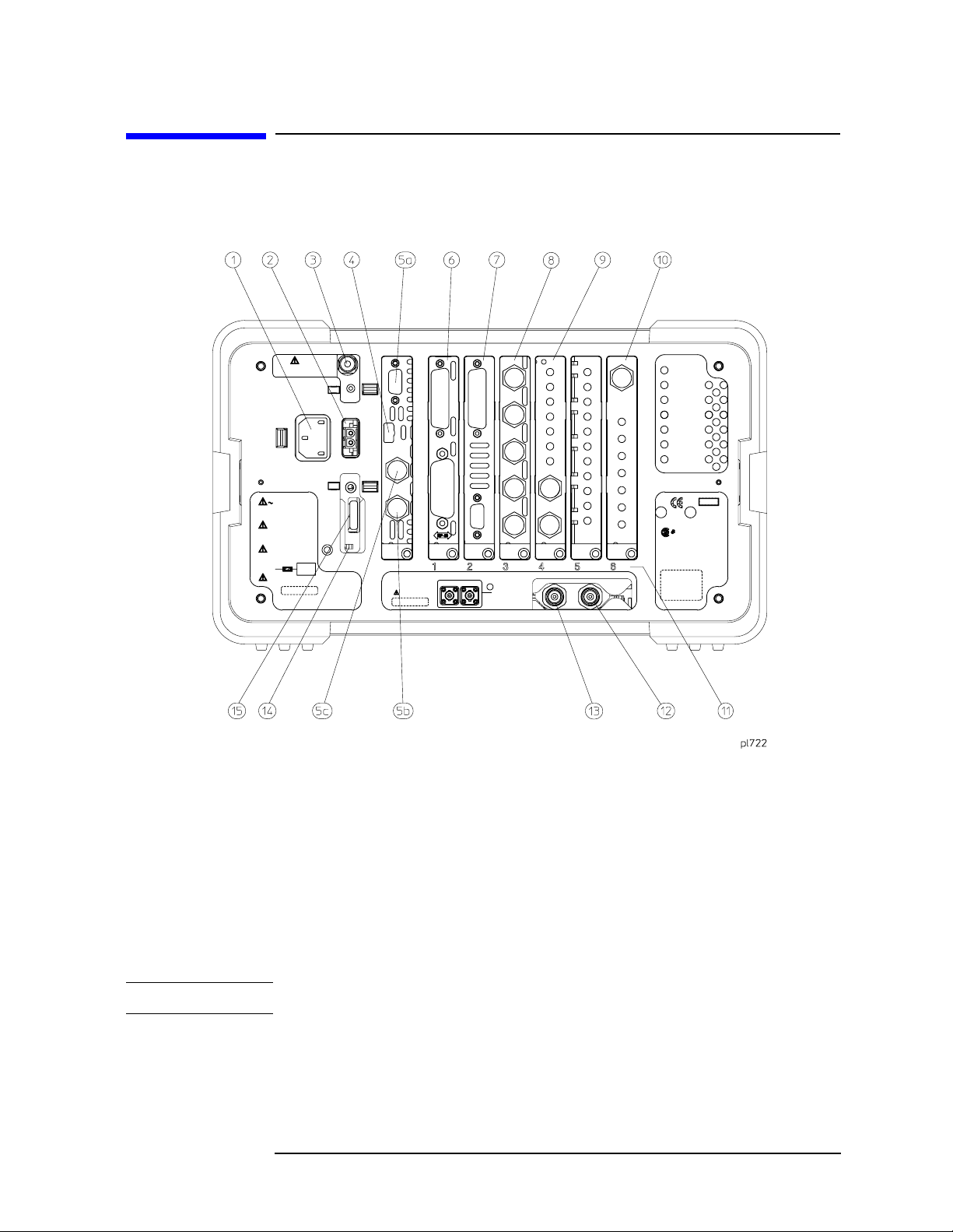
Rear-Panel Features
Figure 1-2 Rear-Panel Feature Overview
Instrument Overview
Rear-Panel Features
1 Power input is the input for the AC line power source.
Make sure that the line-power source outlet has a
protective ground contact.
2 DC Power is the input for the DC power source. Refer to
“Power Requirements” in the Specifications Chapter of
the HP ESA Spectrum Analyzer Calibration
Guide.
CAUTION AC line power and DC power should not be plugged in simultaneously.
3 Line Fuse. The fuse is removed by twisting
counterclockwise 1/4 turn. Replace only with a fuse of
the same rating. See the label on the rear panel.
Chapter 1 1-7

Instrument Overview
Rear-Panel Features
4 Service Connector. The service connector is for service use
only.
5 Inputs/Outputs
5a VGA OUTPUT drives an external VGA
compatible monitor with a signal that
has 31.5 kHz horizontal, 60 Hz vertical
synchronizing rate, non-interlaced.
5b GATE/HI SWP OUT (TTL) indicates when
the analyzer is sweeping.
5c GATETRIG/EXT TRIG IN (TTL) accepts the
positive edge of an external voltage
input that triggers the analyzer
internal sweep source or the gate
function (Time Gate, Option 1D6).
Table2-1 and Table 2-2 show the appropriate rear-panel slots to be used for the
optional cards available with the HP ESA spectrum analyzers. Refer to Table
2-1 if you have an HP ESA-L Series spectrum analyzer. Refer to Table 2-2 if
you have an HP ESA-E Series spectrum analyzer.
(P) = Preferred Card Slot
(A) = Acceptable Card Slot
(–) = Unacceptable Card Slot
Table 1-1 HP ESA-L Series (E4403B, E4408B, E4411B)
Slot # HP-IB
(Opt A4H)
1 PP – – – –
2 AA – – – –
3 –– – – – –
4 –– – – – –
5 –– – P – –
6 –– – – – P
Serial
(Opt 1AX)
FADC
(Opt AYX)
IF and
Sweep
Ports
(Opt A4J)
FM Demod
(Opt BAA)
a. The Frequency Extension Assembly comes standard with the HP E4408B.
Frequency
Extension
a
1-8 Chapter1

Instrument Overview
Rear-Panel Features
Table 1-2 HP ESA-E Series (E4401B, E4402B, E4404B, E4405B, E4407B)
Slot # HP-IB
(Opt A4H)
b
1
2 AA A A A –
3 AA P A A –
4 AA A A P –
5 –– – P A –
6 –– – A A P
PP – A – –
Serial
(Opt 1AX)
FADC
(Opt AYX)
IF and
Sweep
Ports
(Opt A4J)
FM Demod
(Opt BAA)
Frequency
Extension
a
a. The Frequency Extension Assembly comes standard with the HP E4404B,
E4405B and E4407B.
b. The CPU heatsink invades the space allocated to Slot 1. Cards installed in this
space must be “L” shaped to avoid interference.
6 HP-IB and parallel (Option A4H) are optional
interfaces. HP-IB supports remote instrument
operation. The parallel port is for printing only.
7 RS-232 and parallel (Option 1AX) are optional
interfaces. RS-232 supports remote instrument
operation. The parallel port is for printing only.
NOTE Printing is only supported from the parallel port.
NOTE Only one optional interface (Option A4H or Option 1AX) can be
installed at a time.
8 IF and Sweep Ports (Option A4J):
SWP OUT provides a voltage ramp corresponding to the
sweep of the analyzer (0 V to 10 V).
HI SWP IN (TTL) can be grounded to stop sweeping.
HI SWP OUT (TTL) indicates when the analyzer is
sweeping.
AUX VIDEO OUT provides detected video output (before
the analog-to-digital conversion) proportional to
vertical deflection of the trace. Output is from 0 V to
1 V.Amplitude-correction factors are not applied to this
signal. The output signal will be blanked occasionally
during retrace by the automatic alignment routine.
Select a very long sweep time to minimize this, or turn
off the
Auto Align, All function (and use Align Now, All
Chapter 1 1-9

Instrument Overview
Rear-Panel Features
manually to maintain calibration.) Refer to the
Alignments key description in the user’s guide for more
information on alignment key functions.
AUX IF OUT is a 50 Ω, 21.4 MHz IF output that is the
down-converted signal of the RF input of the analyzer.
Amplitude-correction factors are not applied to this
signal. This output is taken after the resolution
bandwidth filters and step gains and before the log
amplifier. The output signal will be blanked
occasionally during retrace by the automatic alignment
routine. Select a very long sweep time to minimize this,
or turn off the
Now, All manually to maintain calibration.) Refer to the
Alignments key description in the user’s guide for more
Auto Align, All function (and use Align
information on alignment key functions.
9 FM Demod (Option BAA) allows you to demodulate,
display, and measure deviation on FM signals. You can
listen to audio signals on a built-in speaker or with an
earphone.
10 Frequency Extension Assembly controls the
microwave front-end components in the HP E4404B,
E4405B, E4407B and E4408B.
11 Card Slot Identification Numbers. Refer to
Table 1-1 and Table 1-2 for card slot versus option card
compatibility information.
12 10 MHz REF IN accepts an external frequency source to
provide the 10 MHz, −15 to +10 dBm frequency
reference used by the analyzer.
13 10 MHz REF OUT provides a 10 MHz, 0 dBm minimum,
timebase reference signal.
14 Power On Selection selects an instrument power
preference. This preference applies after power has
been absent for > 20 seconds. The
PWR NORM position
causes the instrument to remain off when power is
applied. The
on. The
PWR ALWAYS ON position causes it to turn
PWR ALWAYS ON mode is useful if an external
power switch is used to control a rack of several
instruments.
15 DC Fuse protects the analyzer from drawing too much
DC power. Replace only with a fuse of the same rating.
See the label on the rear panel.
1-10 Chapter1

Display Annotation
Here is an example of the annotation that may appear on an analyzer
display. The display annotation is referenced by numbers which are
listed in the following table. The Function Key column indicates which
key activates the function related to the annotation. Refer to the user’s
guide for more information on a specific function key.
Figure 1-3 Screen Annotation
Instrument Overview
Display Annotation
27
26
25
24
23
22
21
20
19
3 4 5 6 987
2
1
10
1211
13
18 17 141516
Table 1-3 Screen Annotation
Item Description Function Key
1 Detector mode Detector
2 Reference level Ref Level
3 Active function block Refer to the description of the
4 Screen title Change Title
5 Time and date display Time/Date On Off
Chapter 1 1-11
pl727
activated function.

Instrument Overview
Display Annotation
Table 1-3 Screen Annotation
Item Description Function Key
6 RF attenuation Attenuation Auto Man
7 Marker frequency Marker Count On Off
8 Marker amplitude Marker
9 HP-IB annunciators RLTS
10 Data invalid indicator Sweep (Single)
See below for more information
11 Pop-up Informational
See the user’s guide.
messages
12 Key menu title Dependent on key selection.
13 Key menu See key label descriptions in the
user’s guide.
14 Frequency span or stop
Span or Stop Freq
frequency
15 Sweep time Sweep Time Auto Man
16 Video bandwidth Video BW Auto Man
17 Frequency offset Freq Offset
18 Display status line Displays instrument status and
error messages.
See the user’s guide.
19 Resolution bandwidth Resolution BW Auto Man
20 Center frequency or start
Center Freq or Start Freq
frequency
21 Auto alignment routine
is on
Auto Align
See below for more information
22 Trigger/Sweep Trig, Sweep
See below for more information
23 Trace mode Trace
24 Video average Video Average On Off
25 Display line Display Line On Off
26 Amplitude offset Ref Lvl Offst
27 Amplitude scale Scale Type Log Lin
1-12 Chapter1

Instrument Overview
Display Annotation
Item 21 refers to the auto alignment mode. AA indicates that auto
alignment of all analyzer parameters, except the tracking generator
and FM demodulation options, will occur. AB indicates that auto
alignment of all analyzer functions except the RF section (and tracking
generator and FM demodulation options) will occur. No indicator will
appear if auto alignment is off.
Item 22 refers to the trigger and sweep modes of the analyzer. The first
letter F indicates the spectrum analyzer is in free-run trigger mode.
The second letter C indicates the spectrum analyzer is in
continuous-sweep mode.
Item 23 refers to the trace modes of the analyzer. The first letter W
indicates that the analyzer is in clear-write mode. The second letter is
1, representing trace 1. The trace 2 trace mode is S2, indicating trace 2
(2) is in the store-blank mode (S). The trace mode annotation for trace 3
is displayed under the trace mode annotation of trace 1. The trace 3
trace mode is S3, indicating trace 3 (3) is in the store blank mode (S).
A # in front of display annotation indicates that the function is
uncoupled.
Refer to the following table for the screen annotation codes for trace,
trigger, and sweep modes.
Table 1-4 Screen Annotation for Trace Mode
Screen Annotation Description
W Clear Write
M Maximum Hold
V View
S Store Blank
m Minimum Hold
Table 1-5 Screen Annotation for Trigger Mode
Screen Annotation Description
F Free Run
L Line
V Video
E External
Chapter 1 1-13

Instrument Overview
Display Annotation
Table 1-6 Screen Annotation for Sweep Mode
Screen Annotation Description
C Continuous
S Single Sweep
Table 1-7 Screen Annotation for HP-IB Annunciators
Screen Annotation Description
R Remote Operation
L HP-IB Listen
T HP-IB Talk
S HP-IB SRQ
1-14 Chapter1

2 Making Basic Measurements
2-1

Making Basic Measurements
What is in This Chapter
What is in This Chapter
This chapter demonstrates basic analyzer measurements with
examples of typical measurements; each measurement focuses on
different functions. The measurement procedures covered in this
chapter are listed below.
• “Comparing Signals” on page 2-3
• “Resolving Signals of Equal Amplitude” on page 2-7
• “Resolving Small Signals Hidden by Large Signals” on page 2-10
• “Making Better Frequency Measurements” on page 2-13
• “Decreasing the Frequency Span Around the Signal” on page 2-15
• “Tracking Drifting Signals” on page 2-17
• “Measuring Low Level Signals” on page 2-21
• “Identifying Distortion Products” on page 2-29
• “Measuring Signal-to-Noise” on page 2-35
• “Making Noise Measurements” on page 2-37
• “Demodulating AM Signals (Using the Analyzer As a Fixed Tuned
Receiver)” on page 2-44
• “Demodulating FM Signals (Without Option BAA)” on page 2-47
To find descriptions of specific analyzer functions, refer to the user’s
guide.
2-2 Chapter2

Making Basic Measurements
Comparing Signals
Comparing Signals
Using the analyzer, you can easily compare frequency and amplitude
differences between signals, such as radio or television signal spectra.
The analyzer delta marker function lets you compare two signals when
both appear on the screen at one time or when only one appears on the
screen.
Example 1:
Measure the differences between two signals on the same display
screen.
1. Connect the 10 MHz REF OUT from the rear panel to the
front-panel INPUT.
2. Set the center frequency to 30 MHz and the span to 50 MHz by
pressing
FREQUENCY, 30 MHz, SPAN, 50 MHz.
3. Set the reference level to 10 dBm by pressing
The 10 MHz reference signal and its harmonics appear on the
display.
4. Press
(The
Search to place a marker at the highest peak on the display.
Next Pk Right and Next Pk Left softkeys are available to move the
marker from peak to peak.) The marker should be on the 10 MHz
reference signal. See Figure 2-1.
Figure 2-1 Placing a Marker on the 10 MHz Signal
AMPLITUDE, 10 dBm.
Chapter 2 2-3

Making Basic Measurements
Comparing Signals
5. Press Marker, Delta, to activate a second marker at the position of the
first marker. Move the second marker to another signal peak using
the knob, or by pressing
Search and Next Pk Right or Next Pk Left.
6. The amplitude and frequency difference between the markers is
displayed in the active function block and in the upper right corner
of the screen. See Figure 2-2. The resolution of the marker readings
can be increased by turning on the frequency count function. Press
Freq Count. Both signals are counted.
Press
Marker, Off to turn the markers off.
Figure 2-2 Using the Marker Delta Function
2-4 Chapter2

Making Basic Measurements
Comparing Signals
Example 2:
Measure the frequency and amplitude difference between two signals
that do not appear on the screen at one time. (This technique is useful
for harmonic distortion tests when narrow span and narrow bandwidth
are necessary to measure the low level harmonics.)
1. Connect the 10 MHz REF OUT from the rear panel to the
front-panel INPUT.
2. Set the center frequency to 30 MHz and the span to 50 MHz by
pressing
The 10 MHz reference signal and its harmonics appear on the
display.
FREQUENCY, 30 MHz, SPAN, 50 MHz.
3. Set the reference level to 10 dBm by pressing
4. Press
5. Press
Search to place a marker on the peak.
Marker, Delta to anchor the position of the first marker and
AMPLITUDE, 10 dBm.
activate a second marker.
6. Press FREQUENCY, CF Step Auto Man (Man) to activate the center
frequency step size function, and enter 50 MHz. Press
Center Freq
and the (↑) key to increase the center frequency by 50 MHz. The first
marker remains on the screen at the amplitude of the first signal
peak.
NOTE Changing the reference level changes the marker delta amplitude
readout.
The annotation in the upper right corner of the screen indicates the
amplitude and frequency difference between the two markers. See
Figure 2-3.
7. To turn the markers off, press
Marker, Off.
Chapter 2 2-5

Making Basic Measurements
Comparing Signals
Figure 2-3 Frequency and Amplitude Difference Between Signals
2-6 Chapter2

Making Basic Measurements
Resolving Signals of Equal Amplitude
Resolving Signals of Equal Amplitude
Two equal-amplitude input signals that are close in frequency can
appear as one on the analyzer display. Responding to a single-frequency
signal, a swept-tuned analyzer traces out the shape of the selected
internal IF (intermediate frequency) filter. As you change the filter
bandwidth, you change the width of the displayed response. If a wide
filter is used and two equal-amplitude input signals are close enough in
frequency, then the two signals appear as one. Thus, signal resolution is
determined by the IF filters inside the analyzer.
The bandwidth of the IF filter tells us how close together equal
amplitude signals can be and still be distinguished from each other. The
resolution bandwidth function selects an IF filter setting for a
measurement. Resolution bandwidth is defined as the 3 dB bandwidth
of the filter.
Generally, to resolve two signals of equal amplitude, the resolution
bandwidth must be less than or equal to the frequency separation of the
two signals. If the bandwidth is equal to the separation and the video
bandwidth is less than the resolution bandwidth, a dip of
approximately 3 dB is seen between the peaks of the two equal signals,
and it is clear that more than one signal is present. See Figure 2-5.
In order to keep the analyzer measurement calibrated, sweep time is
automatically set to a value that is inversely proportional to the square
of the resolution bandwidth (for resolution bandwidths ≥ 1kHz). So, if
the resolution bandwidth is reduced by a factor of 10, the sweep time is
increased by a factor of 100 when sweep time and bandwidth settings
are coupled. (Sweep time is proportional to
2
1/BW
.) For shortest
measurement times, use the widest resolution bandwidth that still
permits discrimination of all desired signals.The analyzer allows you to
select from 1 kHz to 3 MHz resolution bandwidths in a 1, 3, 10 sequence
for maximum measurement flexibility.
Option 1DR adds narrower resolution bandwidths, from 10 Hz to
300 Hz, in a 1-3-10 sequence. These bandwidths are digitally
implemented and have a much narrower shape factor than the wider,
analog resolution bandwidths. Also, the autocoupled sweeptimes when
using the digital resolution bandwidths are much faster than analog
bandwidths.
Chapter 2 2-7
Making Basic Measurements
Resolving Signals of Equal Amplitude
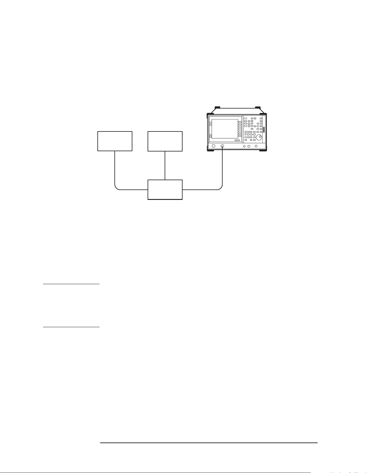
Example:
Resolve two signals of equal amplitude with a frequency separation of
100 kHz.
1. Connect two sources to the analyzer input as shown in Figure 2-4.
Figure 2-4 Setup for Obtaining Two Signals
SOURCE
SOURCE
Input
COUPLER
bn71a
2. Set one source to 300 MHz. Set the frequency of the other source to
300.1 MHz. The amplitude of both signals should be approximately
−20 dBm.
3. On the analyzer, press
Preset. Set the center frequency to 300 MHz,
the span to 2 MHz, and the resolution bandwidth to 300 kHz by
pressing
Resolution BW, 300 kHz. A single signal peak is visible.
NOTE If the signal peak cannot be found, increase the span to 20 MHz by
pressing
FREQUENCY, Signal Track On Off (On), then SPAN, 2 MHz to bring the
signal to center screen. Then press
FREQUENCY, 300 MHz, SPAN, 2 MHz, then BW/Avg,
SPAN, 20 MHz. The signal should be visible. Press Search,
Signal Track On Off so that Off is
underlined to turn the signal track function off.
4. Since the resolution bandwidth must be less than or equal to the
frequency separation of the two signals, a resolution bandwidth of
100 kHz must be used. Change the resolution bandwidth to 100 kHz
by pressing
BW/Avg, 100 kHz. Two signals are now visible as shown in
Figure 2-5. Use the knob or step keys to further reduce the
resolution bandwidth and better resolve the signals.
5. Decrease the video bandwidth to 10 kHz, by pressing
Man (Man) 10 kHz.
2-8 Chapter2
Video BW Auto

Figure 2-5 Resolving Signals of Equal Amplitude
Making Basic Measurements
Resolving Signals of Equal Amplitude
As the resolution bandwidth is decreased, resolution of the individual
signals is improved and the sweep time is increased. For fastest
measurement times, use the widest possible resolution bandwidth.
Under preset conditions, the resolution bandwidth is “coupled” (or
linked) to the span.
Since the resolution bandwidth has been changed from the coupled
value, a # mark appears next to Res BW in the lower-left corner of the
screen, indicating that the resolution bandwidth is uncoupled. (Also see
the
Auto Couple key description in the user’s guide.)
NOTE To resolve two signals of equal amplitude with a frequency separation
of 200 kHz, the resolution bandwidth must be less than the signal
separation, and resolution of 100 kHz must be used. The next larger
filter, 300 kHz, would exceed the 200 kHz separation and would not
resolve the signals.
Chapter 2 2-9
 Loading...