Keysight MXR, EXR User Manual

Download

Keysight Infiniium MXR/EXR-Series Real-Time Oscilloscopes

User's Guide

Notices

CAUTION

WARNING

No part of this manual may be reproduced in any form or by any means (including electronic storage and retrieval or translation into a foreign language) without prior agreement and written consent from Keysight Technologies, Inc. as governed by United States and international copyright laws.

Manual Part Number

54925-97013

Edition

Sixth edition, November 2020

Available in electronic format only

Published by: Keysight Technologies, Inc. 1900 Garden of the Gods Road Colorado Springs, CO 80907 USA

Print History

54925-97000, May 2020

54925-97005, June 2020

54925-97006, November 2020

54925-97010, September 2020

54925-97011, November 2020

54925-97013, November 2020

Warranty

The material contained in this document is provided "as is," and is subject to being changed, without notice, in future editions. Further, to the maximum extent permitted by applicable law, Keysight disclaims all warranties, either express or implied, with regard to this manual and any information contained herein, including but not limited to the implied warranties of merchantability and fitness for a particular purpose. Keysight shall not be liable for errors or for incidental or consequential damages in connection with the furnishing, use, or performance of this document or of any information contained herein. Should Keysight and the user have a separate written agreement with warranty terms covering the material in this document that

conflict with these terms, the warranty terms in the separate agreement shall control.

Technology License

The hardware and/or software described in this document are furnished under a license and may be used or copied only in accordance with the terms of such license.

U.S. Government Rights

The Software is "commercial computer software," as defined by Federal Acquisition Regulation ("FAR") 2.101. Pursuant to FAR

12.212 and 27.405-3 and Department of Defense FAR Supplement ("DFARS")

227.7202, the U.S. government acquires commercial computer software under the same terms by which the software is customarily provided to the public. Accordingly, Keysight provides the Software to U.S. government customers under its standard commercial license, which is embodied in its End User License Agreement (EULA), a copy of which can be found at

www.keysight.com/find/sweula. The

license set forth in the EULA represents the exclusive authority by which the U.S. government may use, modify, distribute, or disclose the Software. The EULA and the license set forth therein, does not require or permit, among other things, that Keysight: (1) Furnish technical information related to commercial computer software or commercial computer software documentation that is not customarily provided to the public; or (2) Relinquish to, or otherwise provide, the government rights in excess of these rights customarily provided to the public to use, modify, reproduce, release, perform, display, or disclose commercial computer software or commercial computer software documentation. No additional government requirements beyond those set forth in the EULA shall apply, except to the extent that those terms, rights, or licenses are explicitly required from all providers of commercial computer software pursuant to the FAR and the DFARS and are set forth specifically in writing elsewhere in the EULA. Keysight shall be under no obligation to update, revise or otherwise modify the Software. With respect to any technical data as defined by FAR 2.101, pursuant to FAR

12.211 and 27.404.2 and DFARS 227.7102, the U.S. government acquires no greater than Limited Rights as defined in FAR 27.401 or DFAR 227.7103-5 (c), as applicable in any technical data.

Safety Notices

This product has been designed and tested in accordance with accepted industry standards, and has been supplied in a safe condition. The documentation contains information and warnings that must be followed by the user to ensure safe operation and to maintain the product in a safe condition.

A CAUTION notice denotes a hazard. It calls attention to an operating procedure, practice, or the like that, if not correctly performed or adhered to, could result in damage to the product or loss of important data. Do not proceed beyond a CAUTION notice until the indicated conditions are fully understood and met.

A WARNING notice denotes a hazard. It calls attention to an operating procedure, practice, or the like that, if not correctly performed or adhered to, could result in personal injury or death. Do not proceed beyond a WARNING notice until the indicated conditions are fully understood and met.

2 Keysight Infiniium MXR/EXR-Series Real-Time Oscilloscopes User's Guide

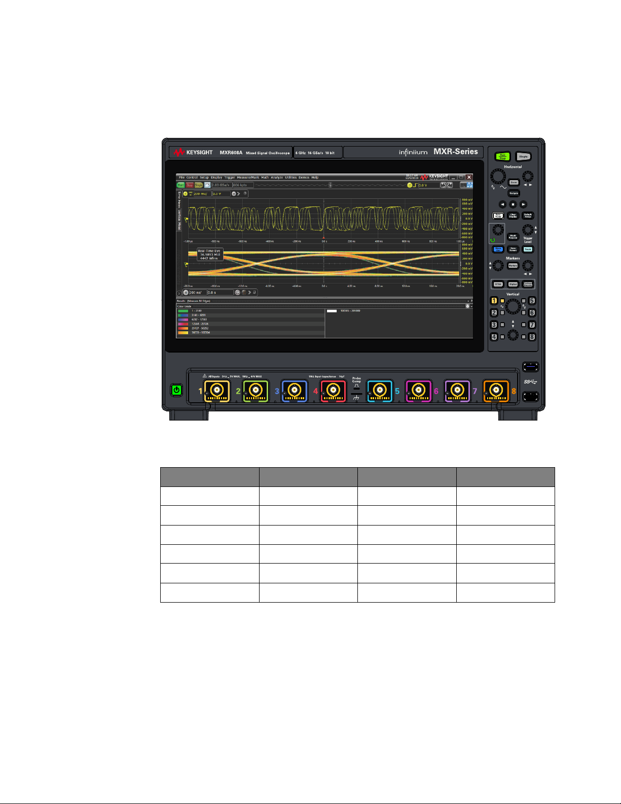
Infiniium MXR/EXR-Series Real-Time Oscilloscopes—At a Glance

+ +

Table 1 Infiniium MXR-Series real-time oscilloscopes

8-Channel Model 4-Channel Model Bandwidth Sampling rate

MXR608A MXR604A 6 GHz 16 GSa/s

MXR408A MXR404A 4 GHz 16 GSa/s

MXR258A MXR254A 2.5 GHz 16 GSa/s

MXR208A MXR204A 2 GHz 16 GSa/s

MXR108A MXR104A 1 GHz 16 GSa/s

MXR058A MXR054A 500 MHz 16 GSa/s

Keysight Infiniium MXR/EXR-Series Real-Time Oscilloscopes User's Guide 3

Table 2 Infiniium EXR-Series real-time oscilloscopes

8-Channel Model 4-Channel Model Bandwidth Sampling rate

EXR258A EXR254A 2.5 GHz 16 GSa/s

EXR208A EXR204A 2 GHz 16 GSa/s

EXR108A EXR104A 1 GHz 16 GSa/s

EXR058A EXR054A 500 MHz 16 GSa/s

In addition to the number of input channels, bandwidths, and sampling rates described in the previous table, the Keysight Infiniium MXR/EXR-Series real-time oscilloscopes deliver these features:

• 10-bit analog-to-digital converter (ADC) with low noise and high effective number of bits (ENOB), with additional high-resolution settings that increase the effective number of bits at lower bandwidths.

• Hardware acceleration and high waveform update rates that make it more likely to capture waveform anomalies.

• 16 digital input channels (1-bit vertical resolution) enabled with the MSO license.

A mixed-signal oscilloscope (MSO) lets you debug your mixed-signal designs using analog signals and tightly correlated digital signals simultaneously. The 16 digital channels have a 8 GSa/s sample rate, with a 400 MHz toggle rate. Thresholds levels can be set per nibble.

• Many trigger modes including: edge, glitch, pulse width, pattern/state, runt, setup and hold, edge transition, edge then edge, timeout, window, OR'd edges, Nth edge, and burst. Also available are sequential triggering and InfiniiScan (Zone triggering and finders for measurements, serial bit streams, runts, and non-monotonic edges).

• Protocol triggering and decode options for many types of protocols including: ARINC-429, BroadR-Reach/100BaseT1, CAN, CAN-FD, eSPI, eUSB2, Ethernet 10BT, Ethernet 100BT, I2C, I2S (LJ, RJ, TDM), LIN, Manchester, MIL-STD 1553, MIPI-I3C, Quad-SPI, RS-232/UART, SENT, Spacewire, SPI, SPMI, SVID, USB

2.0, USB-PD, and more.

• Protocol decode and search options for even more protocols.

• Built-in counter and digital voltmeter (DVM) hardware for the analog input channels.

• Built-in, license-enabled waveform generator with: sine, square, ramp, pulse, DC, noise, sine cardinal, exponential rise, exponential fall, cardiac, Gaussian pulse, PRBS, and demo waveforms output to the GEN OUT side-panel BNC connector. Generated signals can be used to provide stimulus to a device under test (DUT) or for demos.

• Front-panel knobs and keys for: default and autoscale setups, acquisition run control (run, stop, and single), horizontal settings (time/division, trigger

4 Keysight Infiniium MXR/EXR-Series Real-Time Oscilloscopes User's Guide

position, zoom window, and time navigation), vertical settings (scaling down to 1 mV/div in hardware and offset), multiple markers (to check voltage or at any point on a waveform), trigger level, digital channels, protocol decode, clearing acquisitions from the display, and more.

Knobs are pushable for making quick selections.

• 15.6 inch color 1920x1080 (FHD) capacitive touch screen display with multi-touch (gestures), handles, and resizing allows oscilloscope operation without an external pointing device.

• High-capacity removable solid state hard drive for fast boot-up, storing setups, and saving measurement results.

• USB 3.0 and LAN ports make printing, saving, and sharing data easy.

• VGA and DisplayPort ports on the motherboard I/O panel for displaying the screen on a different monitor.

• 64-bit Windows operating system and graphical user interface with familiar menus, toolbars, etc. Ability to install other Windows applications like vector signal analysis (VSA) software.

• Eight analog channel waveform memories and one digital channels waveform memory for comparing with other channels or math waveforms.

• More than 50 automated measurements and measurement statistics.

• Up to 16 math function waveforms selectable from these operations: add, subtract, multiply, divide, d/dt, integrate, invert, FFT magnitude, FFT phase, magnify/duplicate, square, square root, absolute value, low pass filter, high pass filter, averaged value, smoothing, envelope, magnify, maximum, minimum, peak-peak, measurement trend, bus chart, and user-defined functions with MATLAB analysis.

Δ-time

• New analysis tools including: Fault Hunter and Power Analysis.

• Legacy Infiniium analysis tools including: histograms, mask testing (now with multiple masks for separate waveforms), jitter, real-time eye, equalization, crosstalk, and phase noise.

• Supports many compliance testing applications for technologies like: 100BASE-T1, 1000BASE-T1, 10/100/1G Ethernet, 10GBASE-T, 10GBASE-CX4, Broad-R Reach, CPRI, DDR2/LPDDR2, DDR3/LPDDR3, Energy Efficient Ethernet, HDMI, MGBASE-T (2.5G/5G), MIPI C-PHY, MIPI D-PHY, MIPI M-PHY, MOST, NBASE-T (2.5G/5G), OBSAI, ONFI, PCI Express Gen 1-4, Serial RapidIO, TC8 (OPEN), USB 2.0, and XAUI.

Keysight Infiniium MXR/EXR-Series Real-Time Oscilloscopes User's Guide 5

In This Guide

This guide provides the information you need to begin using the Infiniium MXR/EXR-Series real-time oscilloscopes.

Chapter 1, “Setting Up,” starting on page 11, includes unpacking steps, power

and air flow requirements, and other setup information.

Chapter 2, “Getting Started,” starting on page 21, familiarizes you with the inputs

and outputs, front-panel knobs and keys, the graphical user interface, and describes how to perform basic operations with the oscilloscope.

Chapter 3, “Demos and Online Help,” starting on page 49, describes the Infiniium

oscilloscope application's online demos and online help contents. The online help describes in detail how to use the Infiniium oscilloscope.

Chapter 4, “Other Oscilloscope Tasks,” starting on page 53, describes the Infiniium

oscilloscope application's online help contents and online demos. The online help describes how to use the Infiniium oscilloscope application in detail.

Chapter 5, “Calibrating the Oscilloscope,” starting on page 59, describes how to

perform a user calibration.

Chapter 6, “Testing Performance,” starting on page 65, describes the procedures

used to verify that the oscilloscope is operating within specification.

Chapter 7, “Troubleshooting,” starting on page 107, describes what to do if you

encounter any problems with your MXR/EXR-Series oscilloscope.

For More Information

• For detailed information on how to use the oscilloscope, see the Infiniium oscilloscope application's online help. See "Accessing the Online Help" on page 51.

• For information on controlling the oscilloscope from a remote computer, see the Oscilloscopes Programmer's Guide found in the Infiniium oscilloscope application's online help.

For technical assistance, contact your local Keysight Technologies representative at http://www.keysight.com/find/contactus.

6 Keysight Infiniium MXR/EXR-Series Real-Time Oscilloscopes User's Guide

1 Setting Up

Infiniium MXR/EXR-Series Real-Time Oscilloscopes—At a Glance / 3

In This Guide / 6

Inspecting Package Contents / 12

Environmental Characteristics / 13

Positioning for Proper Airflow / 14

Tilting the Oscilloscope for Easier Viewing / 15

Connecting Accessories and a LAN Cable to the Oscilloscope / 16

Connecting Power to the Oscilloscope / 17

Turning On the Oscilloscope / 18

Changing the Administrator Password / 19

2 Getting Started

Front Panel Connectors / 22

Side Panel Connectors / 23

Knobs and Keys on the Front Panel / 26

Channel inputs / 22 Probe compensation terminal / 22

Motherboard I/O / 23 Digital channels connector / 24 GEN OUT / 24 AUX OUT / 24 10 MHz REF IN (50Ω)/24

Maximum input voltage at 10 MHz REF IN input / 24 10 MHz REF OUT (50Ω)/24 AUX TRIG IN (50Ω)/25

Maximum voltage at AUX TRIG IN input / 25 TRIG OUT / 25

Graphical User Interface (GUI) / 28

Keysight Infiniium MXR/EXR-Series Real-Time Oscilloscopes User's Guide 7

Connecting Oscilloscope Probes / 30

Maximum input voltage at analog inputs / 30

Verifying Basic Oscilloscope Operation / 31

Default Setup and Autoscale / 32

Using Default Setup / 32 Using Autoscale / 32

Starting and Stopping Waveform Acquisitions / 33

Clearing the Waveform Display / 33

Adjusting the Horizontal Settings / 35

Adjusting the Horizontal Scale / 35 Adjusting the horizontal trigger position (delay) / 36 Magnifying a part of the waveform using Zoom / 36 Using the Navigate Controls / 37 Setting the scale, position, and timebase reference point / 37

Adjusting the Vertical Settings / 39

Turning an analog channel on or off / 40 Adjusting an analog channel's vertical scale and offset / 40

Trigger Level and Other Controls / 41

Entry Knob / 41 [Multi Purpose] Key / 41 Setting Up Triggers / 42 Waveform Generator / 43 Saving and Printing / 44 Using the Touch Screen / 44

Using Markers / 45

Making Measurements / 46

Using Quick Measurements / 47

Using Digital Channels and Protocol Decode / 48

Controlling Digital Channels / 48 Decoding Serial Protocol Data / 48

3 Demos and Online Help

Using the Demo Wizard / 50

Accessing the Online Help / 51

8 Keysight Infiniium MXR/EXR-Series Real-Time Oscilloscopes User's Guide

4 Other Oscilloscope Tasks

Changing Windows Operating System Settings / 54

Installing Application Programs on Infiniium / 55

Forcing a Default Setup / 56

Hard Drive Recovery / 57

Cleaning the Oscilloscope / 58

5 Calibrating the Oscilloscope

When to Perform a User Calibration / 60

Equipment Required / 61

Calibration Time / 62

Calibration Procedure / 63

6 Testing Performance

Performance Verification General Information / 66

Performance Test Interval / 66 Performance Test Record / 66 Test Order / 66 Test Equipment / 66

Input Impedance Test / 67

Offset Accuracy Test / 69

DC Gain Accuracy Test / 76

Analog Bandwidth—Maximum Frequency Test / 79

Time Scale Accuracy (TSA) Test / 86

Performance Test Record / 89

7 Troubleshooting

Verifying Basic Operation / 108

Before You Contact Keysight / 113

Returning the Oscilloscope to Keysight for Service / 114

Power Up the oscilloscope / 108 Run the oscilloscope self tests / 109 Run the keyboard, LED, and touch screen self tests / 109 Run a user calibration / 112 Verify system performance / 112

Keysight Infiniium MXR/EXR-Series Real-Time Oscilloscopes User's Guide 9

Index

10 Keysight Infiniium MXR/EXR-Series Real-Time Oscilloscopes User's Guide

Keysight Infiniium MXR/EXR-Series Real-Time Oscilloscopes

User's Guide

1 Setting Up

Inspecting Package Contents / 12 Environmental Characteristics / 13 Positioning for Proper Airflow / 14 Tilting the Oscilloscope for Easier Viewing / 15 Connecting Accessories and a LAN Cable to the Oscilloscope / 16 Connecting Power to the Oscilloscope / 17 Turning On the Oscilloscope / 18 Changing the Administrator Password / 19

This chapter shows how to set up and prepare your Infiniium oscilloscope for first-time use.

1 Setting Up

Inspecting Package Contents

✔ Inspect the shipping container for damage.

• Keep the shipping container or cushioning material until you have inspected

the contents of the shipment for completeness and have checked the oscilloscope mechanically and electrically.

• If the shipping container is damaged, or the cushioning materials show signs

of stress, notify the carrier and your Keysight Technologies Sales Office. Keep the shipping materials for the carrier's inspection. The Keysight Technologies Sales Office will arrange for repair or replacement at Keysight's option without waiting for claim settlement.

✔ Inspect the oscilloscope.

If there is mechanical damage or a defect, or if the oscilloscope does not operate properly or does not pass performance tests, notify your Keysight Technologies Sales Office.

✔ Verify that you received the following items in the Infiniium oscilloscope

packaging.

• Infiniium oscilloscope

• Power cord

• Keyboard

• Mouse (USB optical)

• Accessory pouch (mounts on rear of oscilloscope)

• Front panel cover

• Calibration cable

• Quick Start poster

• 500 MHz passive probes (one for each of the analog channel inputs)

• Digital channels cable, BNC probe tip adapter, and 17-channel flying lead

kit (with the MSO option)

If anything is missing, contact your nearest Keysight Technologies Sales Office.

✔ Verify that you received the options and accessories you ordered and that none

were damaged.

For a complete list of options and accessories available for the MXR/EXR-Series real-time oscilloscopes, see:

• Infiniium MXR-Series Real-Time Oscilloscopes Data Sheet

• Infiniium EXR-Series Real-Time Oscilloscopes Data Sheet

12 Keysight Infiniium MXR/EXR-Series Real-Time Oscilloscopes User's Guide

Environmental Characteristics

Environment Indoor use only

Ambient Temperature Operating: +5 °C to +40 °C

Non-operating: –40 °C to +70 °C

CAUTION: If storing the oscilloscope above +40 °C, make sure the flip-out front feet are retracted.

Humidity Operating: maximum relative humidity 80 percent for temperatures up to

31 °C, decreasing linearly to 50 percent relative humidity at 40 °C

Non-operating: up to 95 percent relative humidity, non-condensing, at 40 °C; decreasing linearly to 50 percent relative humidity at 70 °C

Altitude Operating: up to 3,000 meters (9,842 feet)

Non-operating: up to 15,300 meters (50,000 feet)

Weight 32 lbs (14.5 kg)

Setting Up 1

Dimensions Height = 328 mm (12.91 in, with flip-out front feet and handle retracted)

Width = 445 mm (17.52 in)

Depth = 224 mm (8.82 in, including knobs and rear feet)

Safety UL 61010-1:2010/CAN/CSA C22.2 No. 61010-1-12

IEC 61010-1:2017

IEC 61010-2-030:2017

UL 61010-2-030:2018

CAN/CSA-22.2 No. 61010-2-030-17

Installation Category II

Voltage Fluctuations Note that the mains supply voltage fluctuations are not to exceed ±10% of

the nominal supply voltage. Temporary overvoltages may not exceed the allowed voltage fluctuations of +10% nominal.

Pollution Degree The Infiniium MXR/EXR-Series real-time oscilloscopes may be operated in

environments of Pollution Degree 2.

Pollution Degree Definitions

Pollution Degree 1: No pollution or only dry, non-conductive pollution occurs. The pollution has no influence. Example: A clean room or climate-controlled office environment.

Pollution Degree 2. Normally only dry non-conductive pollution occurs. Occasionally a temporary conductivity caused by condensation may occur. Example: General indoor environment.

Pollution Degree 3: Conductive pollution occurs, or dry, non-conductive pollution occurs which becomes conductive due to condensation which is expected. Example: Sheltered outdoor environment.

Keysight Infiniium MXR/EXR-Series Real-Time Oscilloscopes User's Guide 13

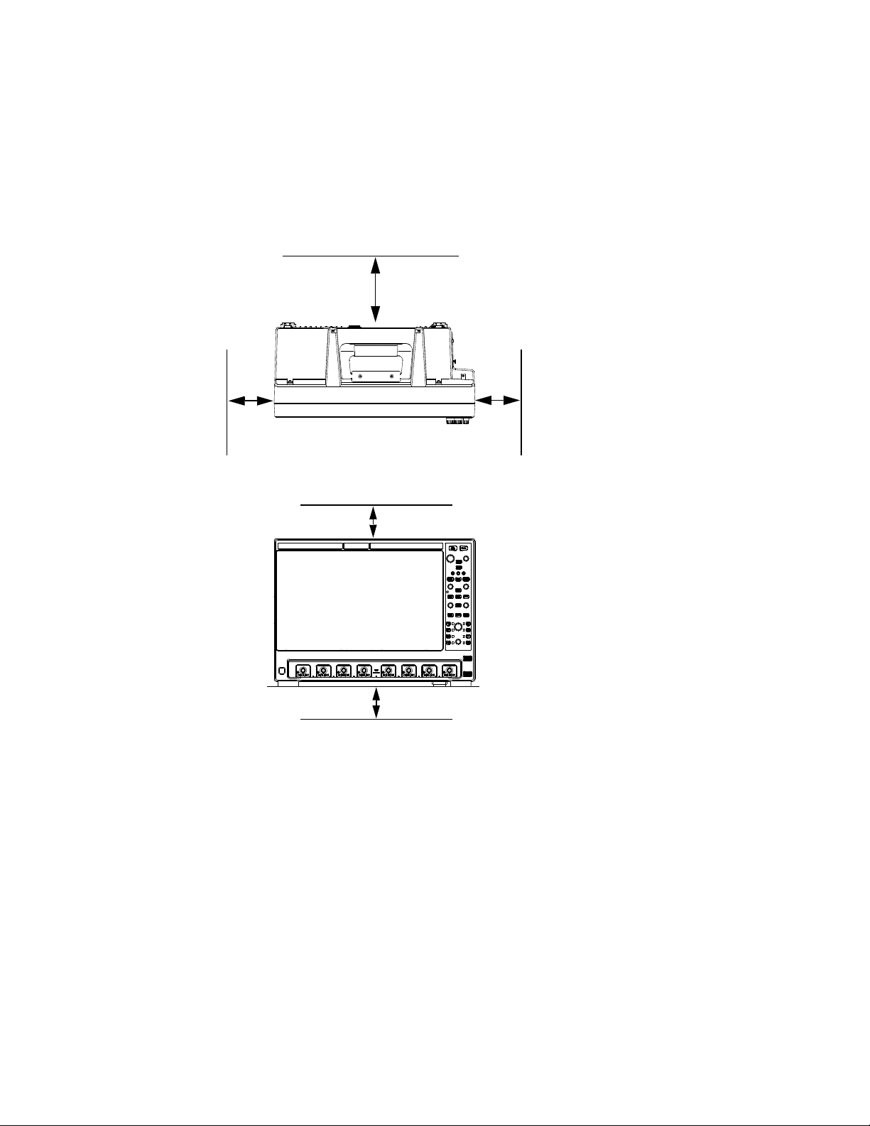
1 Setting Up

Front view

Minimum 0 mm

Minimum 25.4 mm

Minimum bottom clearance: No intrusion into the space under the oscilloscope as defined by the feet. Feet must rest on hard surface.

Top view

Minimum 0 mm

Minimum 25.4 mm

Rear panel

Minimum 75 mm

Positioning for Proper Airflow

Position the oscilloscope where it will have sufficient clearance for airflow around the back and sides.

Figure 1 Positioning the MXR/EXR-Series oscilloscope with sufficient clearance

14 Keysight Infiniium MXR/EXR-Series Real-Time Oscilloscopes User's Guide

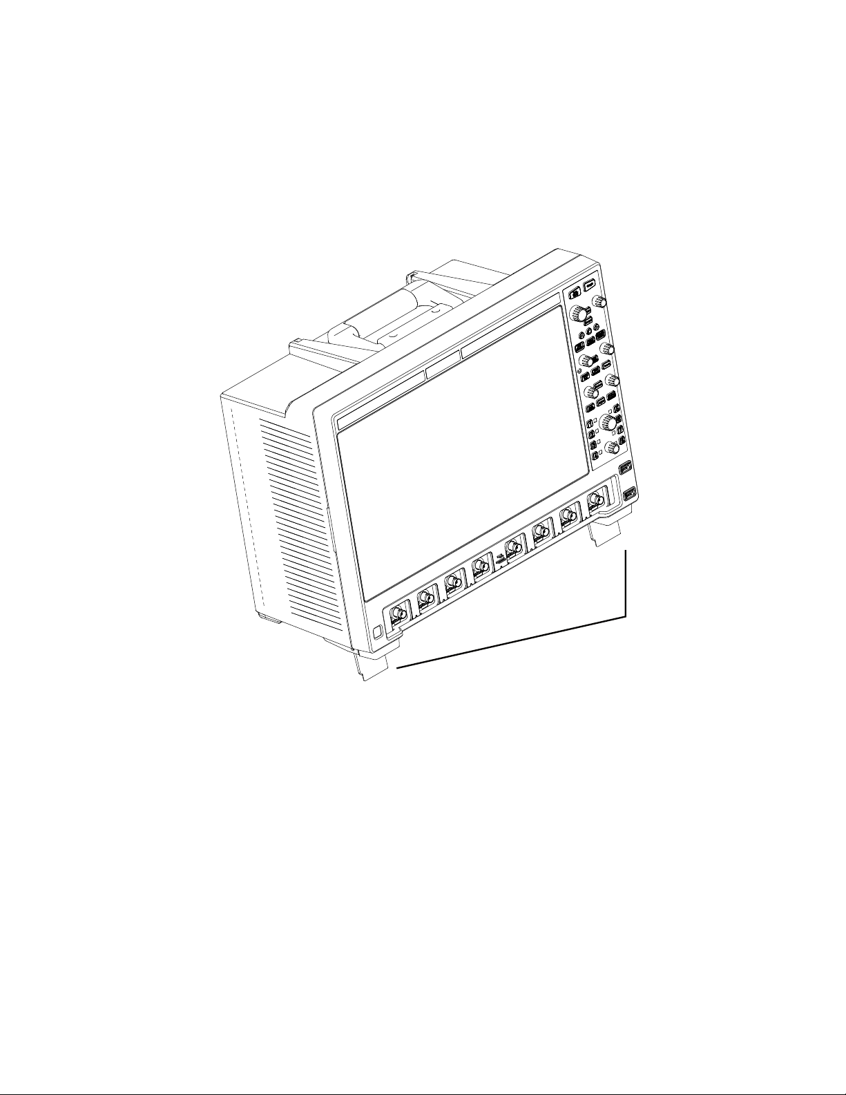
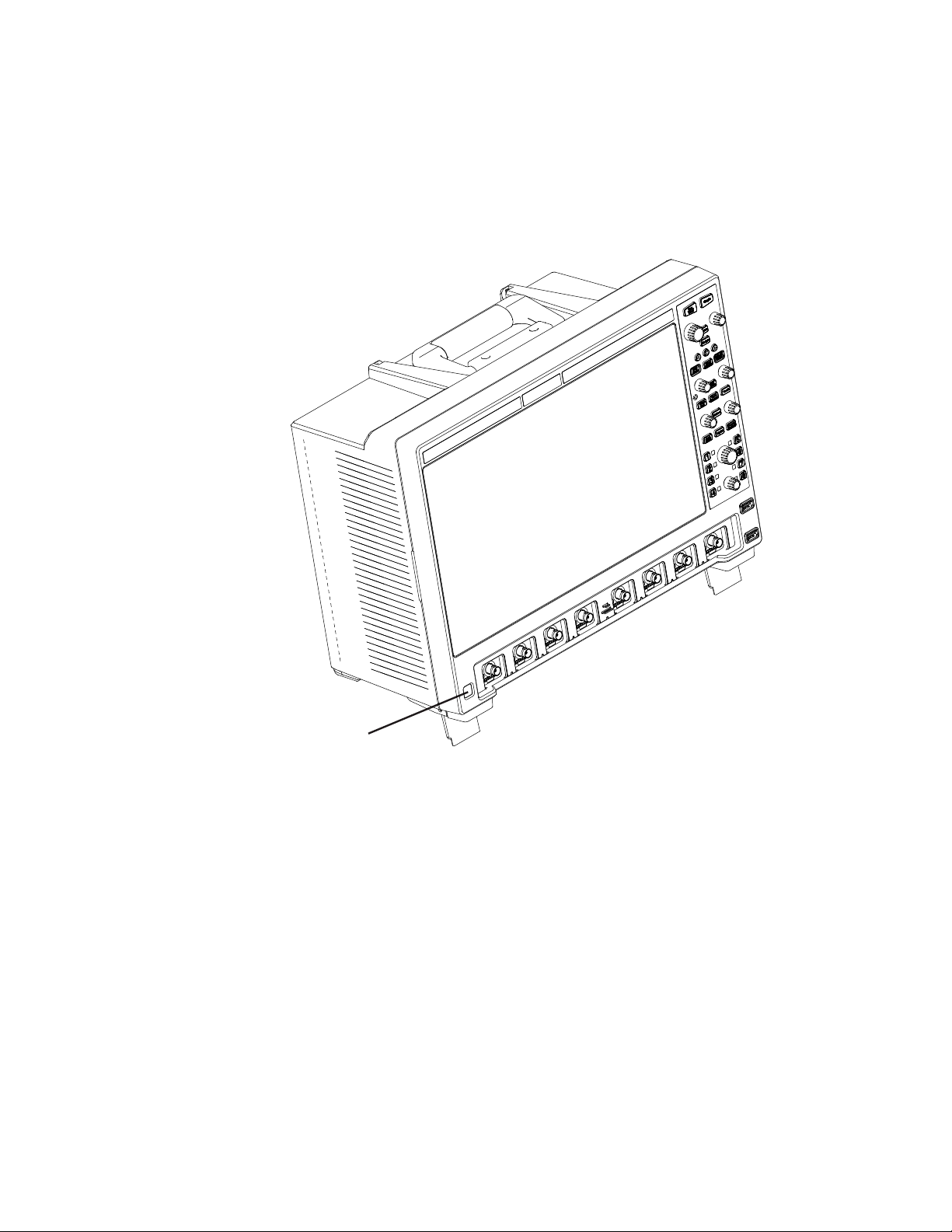
Tilting the Oscilloscope for Easier Viewing

Flip-out tabs

Tabs under the front feet of the oscilloscope can be flipped out to tilt the oscilloscope for easier viewing.

Setting Up 1

Figure 2 Latching the front feet

Keysight Infiniium MXR/EXR-Series Real-Time Oscilloscopes User's Guide 15

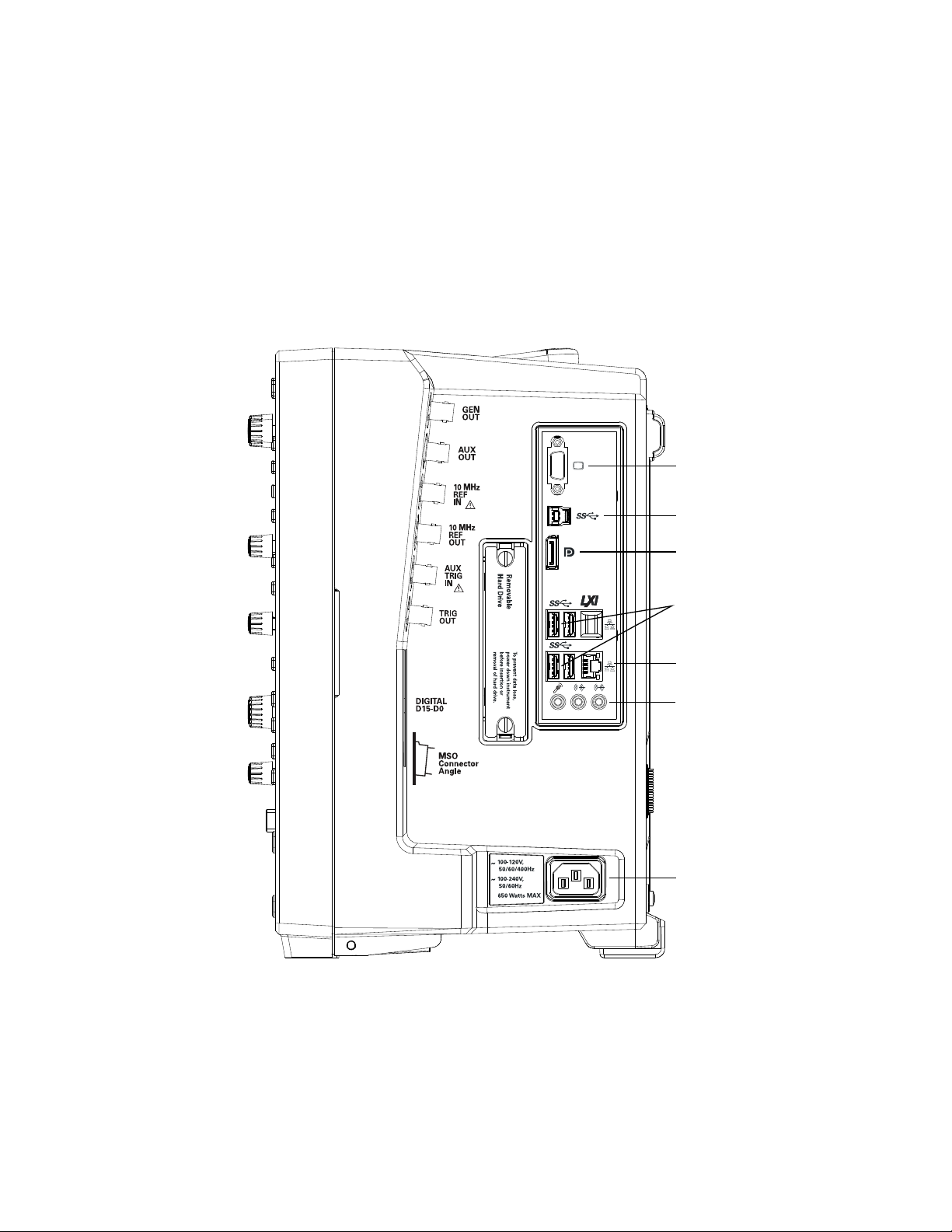
1 Setting Up

Removable

Hard Drive

To prevent data loss,

power down instrument

before insertion or

removal of hard drive.

650 Watts MAX

100-240V,

50/60Hz

100-120V,

50/60/400Hz

10 MH z REF OUT

AUX OUT

IG>< DJI

AUX TRIG IN

GEN OUT

10 MH z REF IN

DIGITAL D15-D0

MSO Connector Angle

External monitor connector

Audio connectors

AC power input

Mouse and keyboard connectors (USB 3 host ports)

LAN connector

DisplayPort

USB 3 Device port

Connecting Accessories and a LAN Cable to the Oscilloscope

1 Plug the mouse and keyboard into the USB host ports. Four host ports are on

the side panel, with two more on the front panel.

2 If you want to connect to a Local Area Network, connect your LAN cable to the

RJ-45 connector on the side panel. Connect the other end to an open LAN port.

Figure 3 Side panel

16 Keysight Infiniium MXR/EXR-Series Real-Time Oscilloscopes User's Guide

Connecting Power to the Oscilloscope

CAUTION

WARNING

Table 3 Power requirements

Power 100-120 V, 50/60/400 Hz

100-240 V, 50/60 Hz

650 W MAX on 8-channel models

450 W MAX on 4-channel models

Connect the power cord to the side of the oscilloscope, then to a suitable AC voltage source. Route the power cord so the oscilloscope's feet do not pinch the cord.

The power cord is the disconnecting device for Mains. Position the equipment so the power cord is easily reached by the operator.

Use only the power cord that came with the oscilloscope

Setting Up 1

The power cord provided is matched to the country of origin of the order.

To avoid electric shock, be sure the oscilloscope is properly grounded.

Keysight Infiniium MXR/EXR-Series Real-Time Oscilloscopes User's Guide 17

1 Setting Up

Turning On the Oscilloscope

Press the power switch in the lower left corner of the oscilloscope front panel.

Figure 4 Turning On the oscilloscope

After a short initialization period, the oscilloscope display appears. The oscilloscope is ready to use.

You can connect and disconnect probes and cables while the oscilloscope is turned on.

Turning Off the

Oscilloscope

To turn the oscilloscope off, press the power switch at the lower left corner of the oscilloscope front panel. The oscilloscope will go through a normal Windows operating system shutdown process.

18 Keysight Infiniium MXR/EXR-Series Real-Time Oscilloscopes User's Guide

Changing the Administrator Password

On Keysight Infiniium MXR/EXR-Series real-time oscilloscopes with the Windows 10 operating system, depending on when the oscilloscope was manufactured, the default Administator user account password is either "keysight4u" or "Keysight4u!". Change the Administrator password to something more secure (and less well-known).

See Also • "Changing Windows Operating System Settings" on page 54

• "Installing Application Programs on Infiniium" on page 55

Setting Up 1

Keysight Infiniium MXR/EXR-Series Real-Time Oscilloscopes User's Guide 19

1 Setting Up

20 Keysight Infiniium MXR/EXR-Series Real-Time Oscilloscopes User's Guide

Keysight Infiniium MXR/EXR-Series Real-Time Oscilloscopes

User's Guide

2 Getting Started

Front Panel Connectors / 22 Side Panel Connectors / 23 Knobs and Keys on the Front Panel / 26 Graphical User Interface (GUI) / 28 Connecting Oscilloscope Probes / 30 Verifying Basic Oscilloscope Operation / 31 Default Setup and Autoscale / 32 Starting and Stopping Waveform Acquisitions / 33 Adjusting the Horizontal Settings / 35 Adjusting the Vertical Settings / 39 Trigger Level and Other Controls / 41 Using Markers / 45 Making Measurements / 46 Using Digital Channels and Protocol Decode / 48

This chapter describes how to use the Infiniium MXR/EXR-Series oscilloscope's inputs and outputs, front panel controls, and user interface.

• The familiar front-panel oscilloscope interface with knobs and keys is optimized for common tasks and basic measurements.

• With the graphical user interface for the Infiniium MXR/EXR-Series oscilloscope you can access all of the oscilloscope's configuration and measurement features through an easy-to-use system of windows, menus, toolbars, dialog boxes, and buttons.

• You have the option of using either the front panel controls or the user interface for many common tasks.

2 Getting Started

~ ~

+ +

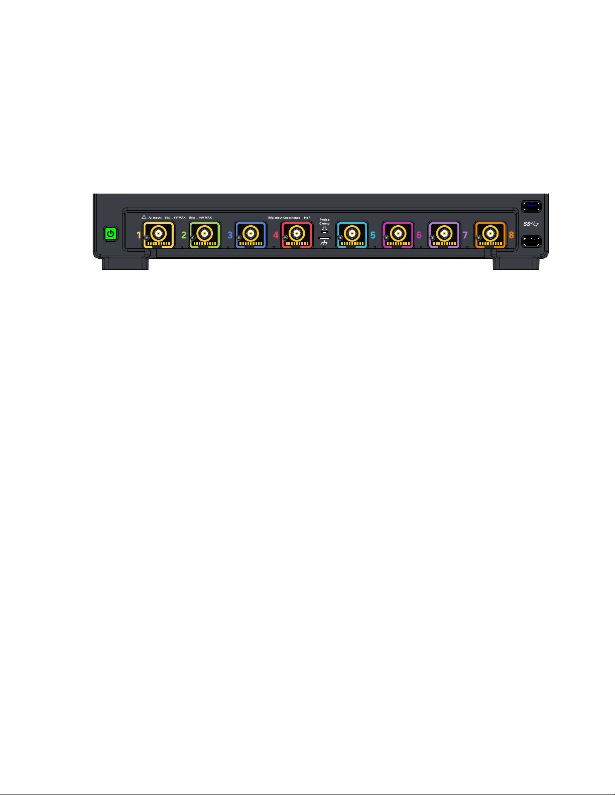
Front Panel Connectors

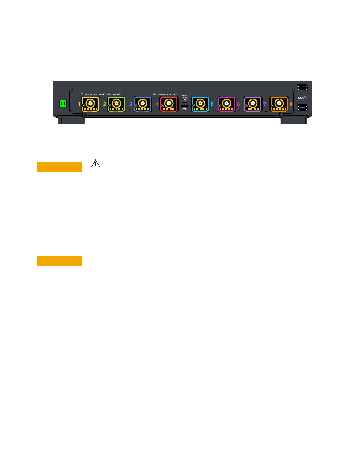
On the Infiniium MXR/EXR-Series oscilloscopes, the channel inputs, probe compensation terminal, and ground lug appear on the lower part of the front panel. Two USB 3.0 host ports are also located here.

Figure 5 Front panel connectors

Channel inputs

Your Infiniium oscilloscope comes with 10:1 500 MHz passive probes for each analog input channel.

The AutoProbe interface also works with the InfiniiMax probing system.

See "Connecting Oscilloscope Probes" on page 30.

Probe compensation terminal

This terminal has a square wave signal that is used to adjust compensated passive probes.

You can also output a DC level on this terminal using the Infiniium oscilloscope application's Calibration Output dialog box (Utilities > Calibration Output...).

22 Keysight Infiniium MXR/EXR-Series Real-Time Oscilloscopes User's Guide

Side Panel Connectors

Removable

Hard Drive

To prevent data loss,

power down instrument

before insertion or

removal of hard drive.

650 Watts MAX

100-240V,

50/60Hz

100-120V,

50/60/400Hz

10 MH z REF OUT

AUX OUT

IG>< DJI

AUX TRIG IN

GEN OUT

10 MH z REF IN

DIGITAL D15-D0

MSO Connector Angle

External monitor connector

Audio connectors

AC power input

Mouse and keyboard connectors (USB 3 host ports)

LAN connector

DisplayPort

USB 3 Device port

The Infiniium MXR/EXR-Series oscilloscope's right side panel has the motherboard I/O connectors, reference clock synchronization connectors, and BNC connectors.

Getting Started 2

Motherboard I/O

Figure 6 Infiniium MXR/EXR-Series oscilloscope side panel I/O

The motherboard provides these inputs/outputs/ports in the oscilloscope: four USB ports for peripherals, an external monitor connector, a USB III device port (for remote control of the oscilloscope from a PC), a LAN port, and speaker and microphone connectors.

Keysight Infiniium MXR/EXR-Series Real-Time Oscilloscopes User's Guide 23

2 Getting Started

CAUTION

Digital channels connector

GEN OUT

AUX OUT

10 MHz REF IN (50Ω)

The MSO option includes a 17-channel flying lead set logic probe, an MSO cable, and a calibration fixture.

Waveform generator signals are output to this BNC connnector. See "Waveform

Generator" on page 43.

This output signal is selected by the Infiniium oscilloscope application's Calibration Output dialog box. It can be a DC level, the probe compensation signal (a square wave used to adjust compensated passive probes), the trigger out signal, or a demo signal.

The 10 MHz REF IN (50Ω) BNC connector is used to synchronize the oscilloscope's horizontal timebase system to a reference clock that you provide.

Maximum input voltage at 10 MHz REF IN input

The clock you provide must meet the following specifications:

• Input frequency lock range: 10 MHz ±20 ppm

• Amplitude, sine wave input: 356 mVpp (-5 dBm) min to 5 Vpp (+18 dBm) max

• Amplitude, square wave input: 285mVpp min to 4Vpp max

• Input impedance: 50Ω (typical)

To use an external reference clock, connect the external clock to the 10 MHz REF IN (50Ω) BNC connector; then, in the Infiniium oscilloscope application's Horizontal dialog box (Setup > Horizontal...), enable the External 10 MHz Reference Clock.

10 MHz REF OUT (50Ω)

You can use the 10 MHz REF OUT (50Ω) BNC connector to send the oscilloscope's 10 MHz reference clock output signal to another instrument's reference clock input.

The output has these characteristics:

• Amplitude into 50Ω (internal or external timebase reference selected): 1.65 ±0.05 Vpp (8.3 ±0.3 dBm) sine wave

24 Keysight Infiniium MXR/EXR-Series Real-Time Oscilloscopes User's Guide

• Frequency accuracy, internal timebase reference selected: 10 MHz ±(8 ppb initial +

CAUTION

75 ppb/year aging)

• Frequency accuracy, external timebase reference selected: external reference frequency (input to 10 MHz REF IN 50Ω)

AUX TRIG IN (50Ω)

You can set up the oscilloscope to trigger on the auxiliary trigger signal connected to this BNC input.

Maximum voltage at AUX TRIG IN input

The input impedance is 50Ω, and the signal you provide must be 5 Vpp maximum between -5 V and +5 V.

TRIG OUT

Getting Started 2

Pulses corresponding to oscilloscope triggers can be sent to this BNC output. TTL levels into a high impedance load are output.

Keysight Infiniium MXR/EXR-Series Real-Time Oscilloscopes User's Guide 25

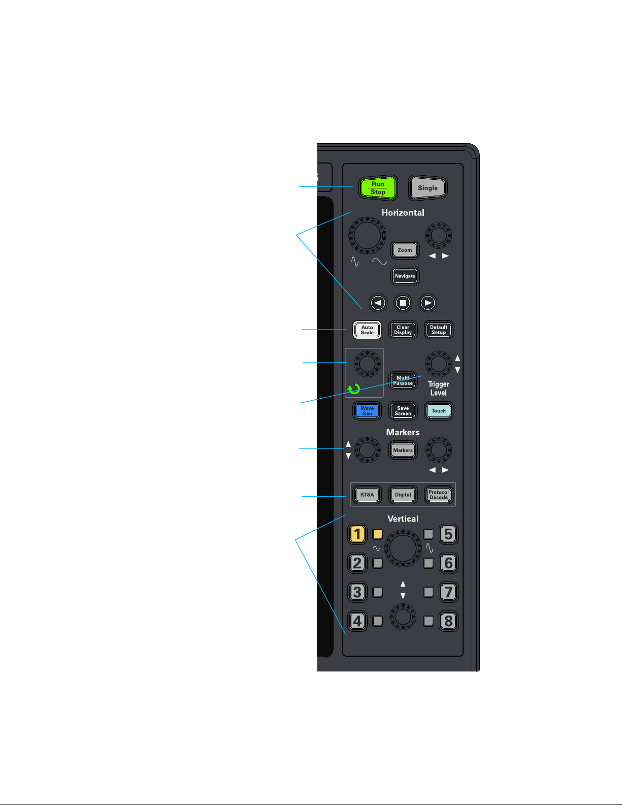
2 Getting Started

Horizontal controls

Entry knob

Vertical controls

Markers controls

Trigger controls

Setup and Display controls

Acquisition run controls

Analysis controls

Knobs and Keys on the Front Panel

Figure 7 Front panel controls

26 Keysight Infiniium MXR/EXR-Series Real-Time Oscilloscopes User's Guide

Getting Started 2

The Infiniium MXR/EXR-Series oscilloscope front panel controls provide direct access to the functions needed to perform the most common measurements. Knobs and keys let you directly set vertical and horizontal parameters. You can see the oscilloscope's configuration at a glance.

The oscilloscope uses color consistently throughout the front panel and user interface. For example, the color of the knob for channel 1 is the same color as the waveform for channel 1. All configuration items and values related to channel 1 are displayed in the same color.

The MXR-Series oscilloscopes have the [RTSA] front panel key for the RTSA (Real-Time Spectrum Analysis) mode. At the same location in the EXR-Series oscilloscopes is the [Fault Hunter] key for the Fault Hunter analysis feature.

Keysight Infiniium MXR/EXR-Series Real-Time Oscilloscopes User's Guide 27

2 Getting Started

Set horizontal scale & position

Open Channel dialog box

Drag/drop measurements

Acquisition run controls

Add waveforms

Customize Results display

Ground indicator

Open Horizontal dialog box

Zoom on/off

Open Add Markers dialog box

Menu bar

Set vertical scale & offset

Clear display Open Acquisition

dialog box

Pin/unpin controls

Memory bar

Open Trigger dialog box

Trigger slope

Set trigger level

Undo/Redo

Grid selection modes:

draw rectangle

drag waveform

Graphical User Interface (GUI)

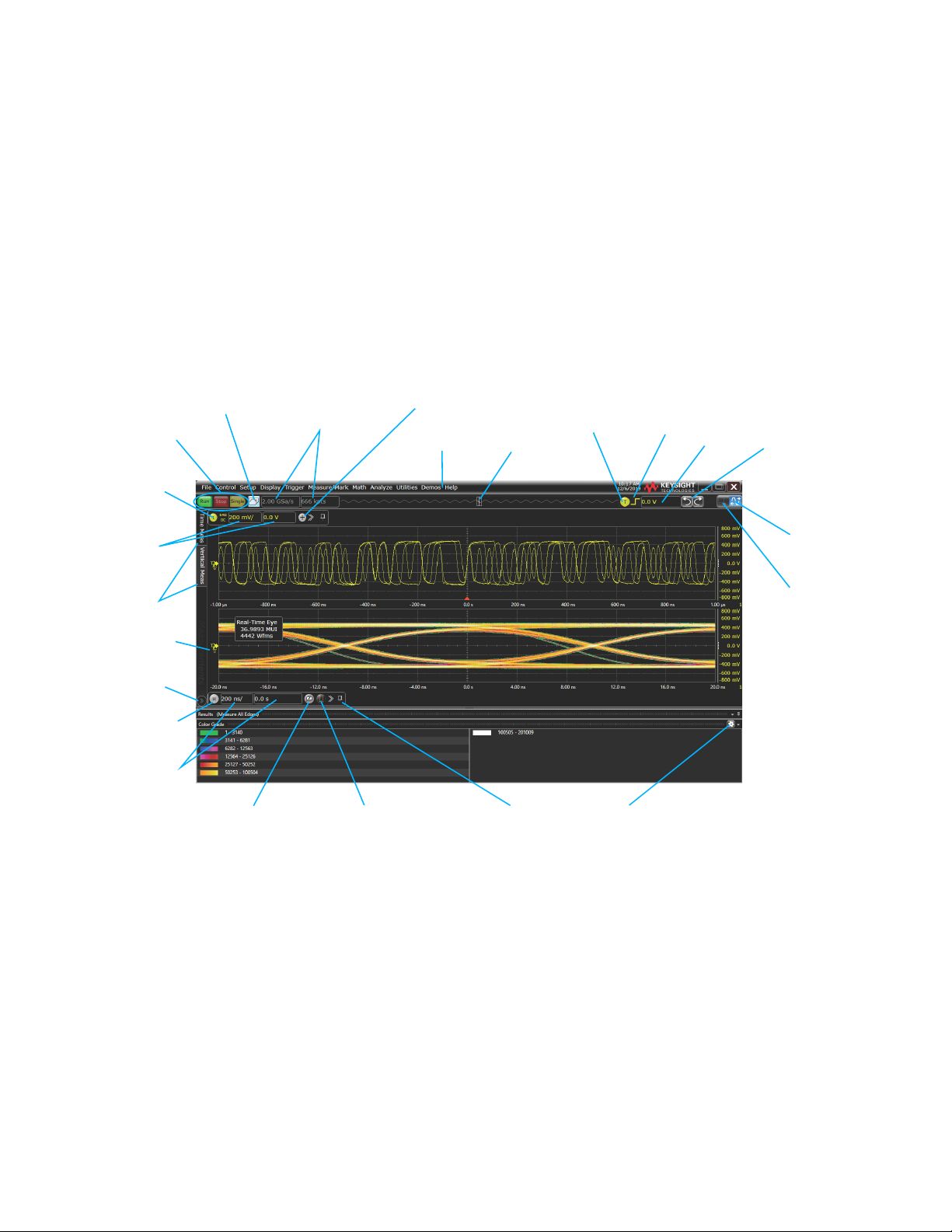
The user interface is arranged so the most common functions affecting the waveform display are located around the edge of the waveform display area.

Context-sensitive menus are available by right-clicking something in the waveform display area, such as a grid, a signal, a bookmark, or a measurement. You can mouse over or touch other areas, such as the drag-and-drop measurements area and horizontal and acquisition control regions, to find more information about those areas or to enter data.

Figure 8 Infiniium oscilloscope display

28 Keysight Infiniium MXR/EXR-Series Real-Time Oscilloscopes User's Guide

Getting Started 2

Table 4 Infiniium oscilloscope display descriptions

Menu bar Use menu selections to perform defined operations and access every

function the oscilloscope provides.

Grid selection modes The selected grid mode determines whether you draw a selection box or

manipulate waveforms when you touch the screen.

Waveform display area The waveform display area shows up to eight waveform windows. Several

display options are available, such as grids or horizontal and vertical scales.

Results pane A Results pane is visible at the bottom of the display when you do

something that produces results, such as taking a measurement or using bookmarks. When it is not needed, the Results pane is not visible.

Keysight Infiniium MXR/EXR-Series Real-Time Oscilloscopes User's Guide 29

2 Getting Started

~ ~

+ +

8 or 4 analog input channels where probes are connected

CAUTION

Connecting Oscilloscope Probes

Figure 9 MXR/EXR-Series oscilloscope probe connectors

Maximum input voltage at analog inputs

Do not exceed the maximum input voltage rating.

The maximum input voltage for the 50 Ω input impedance setting is ±5 V.

The maximum input voltage for the 1 MΩ input impedance setting is 30 Vrms or ±40 Vmax (DC+Vpeak).

Probing technology allows for testing of higher voltages; the included N2873A 10:1 probe supports 300 Vrms or ±400 Vmax (DC+Vpeak). No transient overvoltage allowed. Mains isolated circuits only.

When measuring voltages over 30 V, use a 10:1 probe.

The Keysight Infiniium MXR/EXR-Series oscilloscopes are not rated for Measurement Category II, III, or IV.

For complete documentation on Keysight oscilloscope probes for your Infiniium oscilloscope, see the Probe Resource Center at: keysight.com/find/prc

To connect oscilloscope probes:

1 Attach the probe connector to the desired oscilloscope channel or trigger input

using the probe instructions.

2 Connect the probe to the circuit of interest using the browser or other probing

accessories.

30 Keysight Infiniium MXR/EXR-Series Real-Time Oscilloscopes User's Guide

Verifying Basic Oscilloscope Operation

~ ~

+ +

Front panel connector with square wave label

Channel 1 input

1 Connect one end of the passive probe cable to oscilloscope input channel 1.

2 Connect the other end of the passive probe cable to the front panel Probe

Comp terminal with the square wave label.

Figure 10 Verifying basic oscilloscope operation

Getting Started 2

3 Press [Default Setup] on the front panel.

The display will pause momentarily while the oscilloscope is configured to its default settings. The oscilloscope is now in a known operating condition.

4 Press [Auto Scale] on the front panel.

The display will pause momentarily while the oscilloscope adjusts the time/div setting and vertical scale so the oscilloscope can best display the input signals. You should then see a square wave with about four cycles on screen and a peak-to-peak amplitude of approximately five divisions.

If you do not see the waveform, make sure your power source is adequate, the oscilloscope is properly powered on, and the cable is connected securely to the front panel connector output.

5 Move the mouse around the mouse surface and verify that the on-screen

pointer follows the mouse movement.

6 Press the [Touch] key on the front panel to turn on the touch screen. Press and

hold your finger to the screen. A right-click menu appears, which verifies that the touch screen is working properly.

Keysight Infiniium MXR/EXR-Series Real-Time Oscilloscopes User's Guide 31

2 Getting Started

NOTE

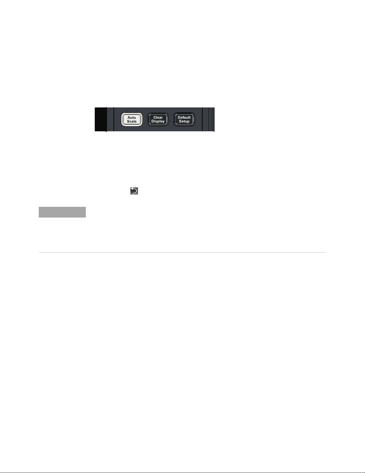
Default Setup and Autoscale

With the setup and display controls you can quickly get a stable waveform display, clear the display, and set the oscilloscope to a known starting condition.

Figure 11 [Auto Scale] and [Default Setup] keys

Using Default Setup

To reset the oscilloscope to its default setup, press [Default Setup]. You can use the

Undo button to undo a default setup.

Save the Current Oscilloscope Configuration

Before using the default setup, you may want to save the current oscilloscope configuration for later use. See the online help for instructions on saving setups, and for information on the exact configuration that is set when you use the default setup. See "Accessing the Online

Help" on page 51.

Using Autoscale

To automatically configure the oscilloscope to best display the current input signal(s), press [Auto Scale] or choose Control > Autoscale.

32 Keysight Infiniium MXR/EXR-Series Real-Time Oscilloscopes User's Guide

Starting and Stopping Waveform Acquisitions

Use the acquisition run controls to run and stop acquisitions or make a single acquisition. The boxed area of the memory bar above the waveform display area shows which portion of the channel's acquisition memory you are viewing.

Figure 12 Acquisition run control keys and buttons

•To start waveform acquisition, press [Run/Stop] or click Run.

Getting Started 2

The oscilloscope begins acquiring data. When the event that triggers the oscilloscope is found (or, in the Auto sweep mode when a good amout of time has elaped without the trigger event — see "Setting Up Triggers" on page 42), the oscilloscope finishes acquiring data, updates the display, and then starts another acquisition cycle.

•To stop waveform acquisition, press [Run/Stop] or click Stop. Data that was last acquired remains on the screen.

• To make a single acquisition, press [Single] or click Single.

• You can also choose the Run, Stop, and Single commands from the Control menu.

• To set up how you want the signals to be sampled, such as sampling rate and

mode, choose Setup > Acquisition....

Clearing the Waveform Display

Figure 13 [Clear Display] key

Keysight Infiniium MXR/EXR-Series Real-Time Oscilloscopes User's Guide 33

2 Getting Started

When you press [Clear Display] or click , the oscilloscope clears acquired waveform data from the display in preparation for another acquisition. If the oscilloscope is in Run mode and is receiving triggers, it will update the display as it collects new waveform data.

Clearing the waveform display also resets averaging, infinite persistence, color grade persistence, histograms, and the mask testing database.

34 Keysight Infiniium MXR/EXR-Series Real-Time Oscilloscopes User's Guide

Adjusting the Horizontal Settings

Horizontal position knob

Horizontal scale knob

Magnify part of the waveform in a new window

Turn Zoom mode on/off

Set horizontal scale (time per division)

Set horizontal position (delay)

Use the horizontal controls to configure the horizontal scale and horizontal position of the waveform. You can view a magnified section of the waveform using the zoom window.

To adjust the horizontal scale and position, use gestures on the touch screen or use the horizontal knobs, horizontal controls, or Horizontal dialog box.

Adjusting the Horizontal Scale

Getting Started 2

Figure 14 Front panel horizontal knobs and controls

Figure 15 Graphical user interface horizontal controls

• The horizontal scale knob is the larger of the two horizontal control knobs. To stretch the waveform horizontally (displaying fewer seconds per division), turn the knob clockwise. To shrink it horizontally, turn the knob counter-clockwise.

• Push and turn the horizontal scale knob to change the scaling in finer (Vernier) increments.

• You can also use multi-touch gestures to stretch or shrink the waveform.

Keysight Infiniium MXR/EXR-Series Real-Time Oscilloscopes User's Guide 35

2 Getting Started

NOTE

Adjusting the horizontal trigger position (delay)

• To adjust the horizontal scale using the controls in the horizontal toolbar, mouse over or touch the horizontal scale field and use the resulting controls to set a particular horizontal scale. Click the scale field to enter an exact value, or click the "narrower" or "wider" buttons.

• The horizontal position knob is the smaller of the two horizontal control knobs. Turn the knob to move the waveform to the right or left.

• Moving the waveform to the right shows more of the pre-trigger data (data acquired before the trigger event). Moving it to the left shows more post-trigger data.

• When you drag a waveform, the horizontal position will change for all channels and functions on the display. Waveform memories will also move if you select the Tie to Timebase box in the Waveform Memories dialog box.

• To adjust the horizontal position using the controls in the horizontal toolbar, mouse over or touch the horizontal position field and use the resulting controls to set a particular horizontal position (time relative to the trigger at the highlighted horizontal reference point).

Magnifying a part of the waveform using Zoom

• To turn on zoom, press the key or click the Zoom button .

The waveform display area splits into two regions. The top one is the main timebase. The bottom is the zoomed timebase, which represents an expansion of the acquired waveform data. A section of the waveform in the main timebase window is highlighted to indicate the part shown in the zoomed timebase window.

The horizontal scale and position controls now change how the waveform is shown in the zoomed timebase window. The horizontal scale will change the amount of magnification, while the position will change the part of the waveform in the main window that is shown in the zoomed window.

• To turn off zoom, press or click again.

Avoid Overdriving Vertical Input Amplifiers

When zooming on a waveform with the oscilloscope running, be careful to keep the signal within the screen vertically to avoid overdriving the vertical input amplifiers. Overdriving causes waveform distortion and erroneous measurement results.

"ADC clipping" indicators appear when a signal exceeds the input voltage range of the ADC. These indicators can sometimes appear when a signal appears to be within the vertical range of the screen due to DSP filtering, but it really is not.

36 Keysight Infiniium MXR/EXR-Series Real-Time Oscilloscopes User's Guide

Using the Navigate Controls

Navigation can be performed for acquisition history (which is available when running acquisitions are stopped), time, segmented memory acquisitions, protocol search, measurement limit test, and mask test.

The [Navigate] key opens the Navigate dialog box where you can choose what to navigate.

Press the navigation keys to step or play backward, stop (when navigation is being played), or step or play forward. When playing, you can press

Getting Started 2

the or keys multiple times to speed up the playback. There are three speed levels.

Additionally, the graphical user interface provides first and last buttons for

navigating to the first or last item in the collection, and somtimes there is a play button for playing items.

The navigation controls also appear in the horizontal controls bar and can be displayed or hidden by clicking the clock button.

Setting the scale, position, and timebase reference point

To set scale, position, and timebase reference, use the Horizontal dialog box or set up the zoomed timebase window.

To access the Horizontal dialog box, click the in the horizontal toolbar, or choose Setup > Horizontal... from the main menu.

Keysight Infiniium MXR/EXR-Series Real-Time Oscilloscopes User's Guide 37

2 Getting Started

The Timebase Reference range is from 0 to 100% of the screen. The center of the screen is at 50%. The slider correlates to the hollow orange triangle at the bottom of the display area, showing where the horizontal offset is on the screen.

38 Keysight Infiniium MXR/EXR-Series Real-Time Oscilloscopes User's Guide

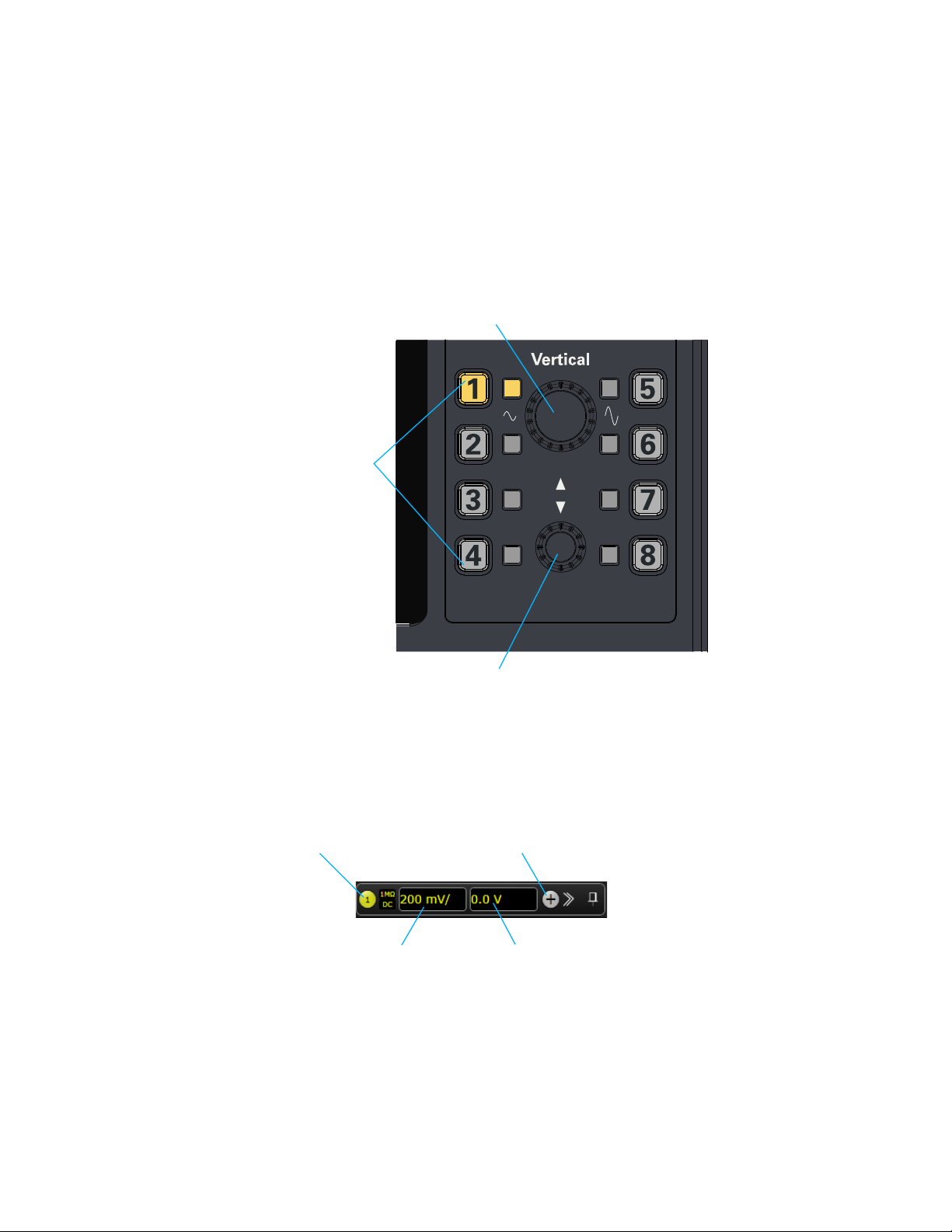
Adjusting the Vertical Settings

Vertical offset knob: adjusts vertical offset (position) of selected channel

Vertical scale knob: adjusts vertical scale of selected channel

Turn waveforms on/off

Set vertical scale Set vertical offset

Use the vertical controls to set the vertical scaling and vertical offset for each analog channel, and to turn the display on or off for a specific channel.

Getting Started 2

Figure 16 Front panel vertical controls

Figure 17 Graphical user interface vertical controls

Keysight Infiniium MXR/EXR-Series Real-Time Oscilloscopes User's Guide 39

2 Getting Started

NOTE

Turning an analog channel on or off

Adjusting an analog channel's vertical scale and offset

To turn an analog channel on or off, press the channel number key on the front

panel or click the Add Waveforms button . When you turn off a channel, the current vertical scale and offset fields for that channel disappear.

If you are not using a particular analog channel, you can turn it off to simplify the waveform display and increase the display update rate. Functions continue to run on a channel source that is turned off. Data acquisition continues for a channel if a function requires it.

Using an Analog Channel as Trigger

Any analog channel can be used as a trigger source. If you need a trigger but do not need all analog channels, you can use an analog channel as a trigger without displaying it by turning the analog channel display off.

To adjust the vertical scale and offset, use the vertical scale and offset knobs, vertical user interface controls, or Channel dialog box.

The vertical scale knob is the larger of the two knobs for a channel. Turn the knob to make the waveform bigger (fewer volts per division) or smaller. You can also mouse over or touch the vertical scale field and use the resulting controls to set an exact value for the scaling.

The vertical offset knob is the smaller knob for a channel. Turn it to move the waveform up or down.

You can drag the waveform or its ground reference indicator to the desired vertical

offset if the grid is in drag mode .

Choose Setup > Channel N... or click a channel number to open the Channel dialog box, in which you can set the vertical scale, offset, skew, and labels. You can also specify the characteristics of a probe, or perform a probe calibration.

For Keysight Technologies probes that are compatible with the AutoProbe interface, the oscilloscope will automatically set these characteristics (except for skew) after identifying the probe when it is connected to the channel input.

40 Keysight Infiniium MXR/EXR-Series Real-Time Oscilloscopes User's Guide

Trigger Level and Other Controls

Set trigger level

Entry knob

Press to perform configured action (like Quick Meas)

Enable/disable touch screen

Enable/disable waveform generator output

Capture screen, save to hard drive

Around the Trigger Level knob, centrally located on the front panel, are controls for performing various tasks.

Getting Started 2

Figure 18 Front panel trigger level (and other) controls

Entry Knob

The Entry knob is a multiplexed knob that can used to adjust values in selected dialog box fields.

The curved arrow LED on the front panel illuminates whenever the Entry knob can be used to adjust a value. The value being adjusted is displayed in a popup message box.

Also, when the symbol appears in a field, you can use the Entry knob to adjust values.

The Entry knob can sometimed be pushed to make a selection or default value setting.

[Multi Purpose] Key

The [Multi Purpose] key can be configured to perform one of many quick actions, such as loading a setup file, saving composite data or a measurement report to a file, saving the screen image to a bitmap file, or performing automatic measurements.

Keysight Infiniium MXR/EXR-Series Real-Time Oscilloscopes User's Guide 41

2 Getting Started

Setting Up Triggers

The action taken when [Multi Purpose] is pressed (or when Utilities > Multipurpose is chosen) depends on the feature selected in the Customize Multipurpose dialog box (Utilities > Customize Multipurpose...).

Use the graphical user interface trigger controls to set the conditions on which the oscilloscope will trigger and acquire an input signal. You can set up a variety of trigger conditions.

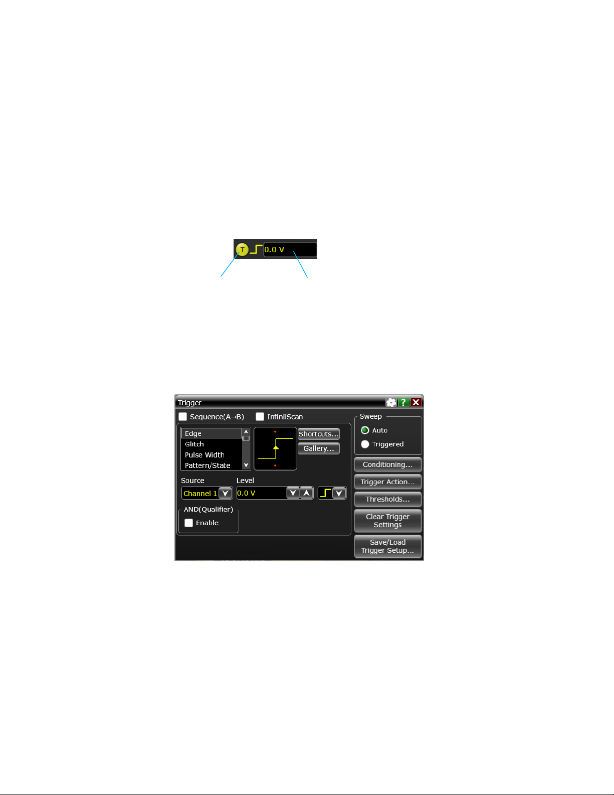
Figure 19 Graphical user interface trigger controls

For example, to set up an Edge trigger:

1 Click the T button in the graphical user interface to open the Trigger dialog box.

2 In the Trigger dialog box, select the Edge trigger type. 3 Select the Source .

You can choose any channel or the Aux (AUX TRIG IN) or Line (the 50% level of the oscilloscope's AC power source signal) input as the source for an edge trigger.

4 Enter the voltage level at which the oscilloscope will trigger either by using the

Level field or by turning the Trigger Level knob.

5 Select a rising edge, falling edge, or both edges slope to trigger on. 6 Select the desired Sweep:

42 Keysight Infiniium MXR/EXR-Series Real-Time Oscilloscopes User's Guide

• When Triggered is selected, the oscilloscope must find the trigger before

saving and displaying captured data.

• When Auto is selected, if a trigger does not occur within a certain amount of

time, an acquisition is automatically saved and displayed. In Auto trigger mode, you are able to see your signals while setting up the desired trigger.

Use the Trigger dialog box to select any of the modes of triggering, the parameters and conditions for each trigger mode, and advanced configuration items.

You can also mouse over the Trigger Level field and use the resulting controls to set a particular trigger level when the oscilloscope is set for edge trigger on a particular channel. You can drag the trigger reference indicator at the left side of the display, or drag the trigger line itself, which appears when you click or touch the grid.

Waveform Generator

The built-in license-enabled waveform generator can output sine, square, ramp, pulse, DC, noise, sine cardinal, exponential rise, exponential fall, cardiac, Gaussian pulse, PRBS, and demo waveforms on the GEN OUT output.

Getting Started 2

Noise can be added to all waveform types except: noise and demo.

AM, FM, or FSK modulation can be performed on all waveform types except: square, pulse, DC, noise, Gaussian pulse, and demo.

The [Wave Gen] key enables or disables the waveform output on GEN OUT.

To select the waveform type and its parameters in the graphical user interface, choose Setup > Waveform Generator... to open the Waveform Generator dialog box.

Keysight Infiniium MXR/EXR-Series Real-Time Oscilloscopes User's Guide 43

2 Getting Started

Saving and Printing

Using the Touch Screen

You can press the [Save Screen] key to capture and save a screen image to the oscilloscope's hard drive in the C:\Users\Public\Documents\Infiniium\Screen Images\ folder.

In the graphical user interface, you can:

•Choose File > Save > and use the menu selections to save composite files (setups and waveforms), setup files, waveform data, screen images, or measurement data. You can also save waveforms to waveform memoriies.

•Choose File > Copy Screen Image to easily copy and paste a screen image into a document.

•Choose File > Print... to send screen images and setup data to a specified printer.

Note that you can customize the [Multi Purpose] key to perform a QuickPrint.

1 To enable the touch screen so it responds to multi-touch gestures, similar to

those used on tablets and smart phones, press [Touch] or choose Utilities > User Preferences... and select the Enable Touch Screen check box.

2 Touch the drag waveform icon to highlight it.

Now you can use gestures to flick items horizontally, drag a waveform vertically, drag horizontally to change the horizontal delay, pinch horizontally to adjust time/div and delay settings, pinch vertically to adjust a waveform's V/div and offset settings, or tap to select waveforms and other selections on the display.

44 Keysight Infiniium MXR/EXR-Series Real-Time Oscilloscopes User's Guide

Using Markers

Open Markers dialog box

Turn to move a marker; push to change the marker

Getting Started 2

Use the Markers controls to display and adjust markers.

Markers make it easier to make precise measurements because the marker measurement readouts show exact voltage and time positions for the markers. The measurements are based on actual waveform data from the acquisition system, not on approximations based on the display position, so you can be sure the values are highly accurate.

Using the markers controls, you can control multiple sets of markers within the oscilloscope grid.

Figure 20 Front panel markers controls

Both time and voltage differences between the markers are updated continuously on the screen. By default, the markers track the source waveform. Voltage measurements from the markers are the value of the waveform at the time set with the marker arrow keys.

• To add a marker, press the [Markers] key or choose Measure/Mark > Add Markers...

or click the Markers button ; then, select the sources and mode.

Notice the drawing in the Mode area of the Marker dialog box.

• To select one of the markers, push one of the marker Position knobs. Turn the knob to move the marker. Push the knob again to select the next marker.

• Marker 1 has a solid line pattern on the waveform display. It is associated with the first available source on the display.

• You can drag a marker to quickly move to the position you want on the waveform.

• You can use the front panel Position knob for fine adjustment, or use the Add Marker dialog box to set the marker position precisely.

Keysight Infiniium MXR/EXR-Series Real-Time Oscilloscopes User's Guide 45

2 Getting Started

Expand and collapse the measurement icons

Drag and drop measurement icons showing most commonly used measurements

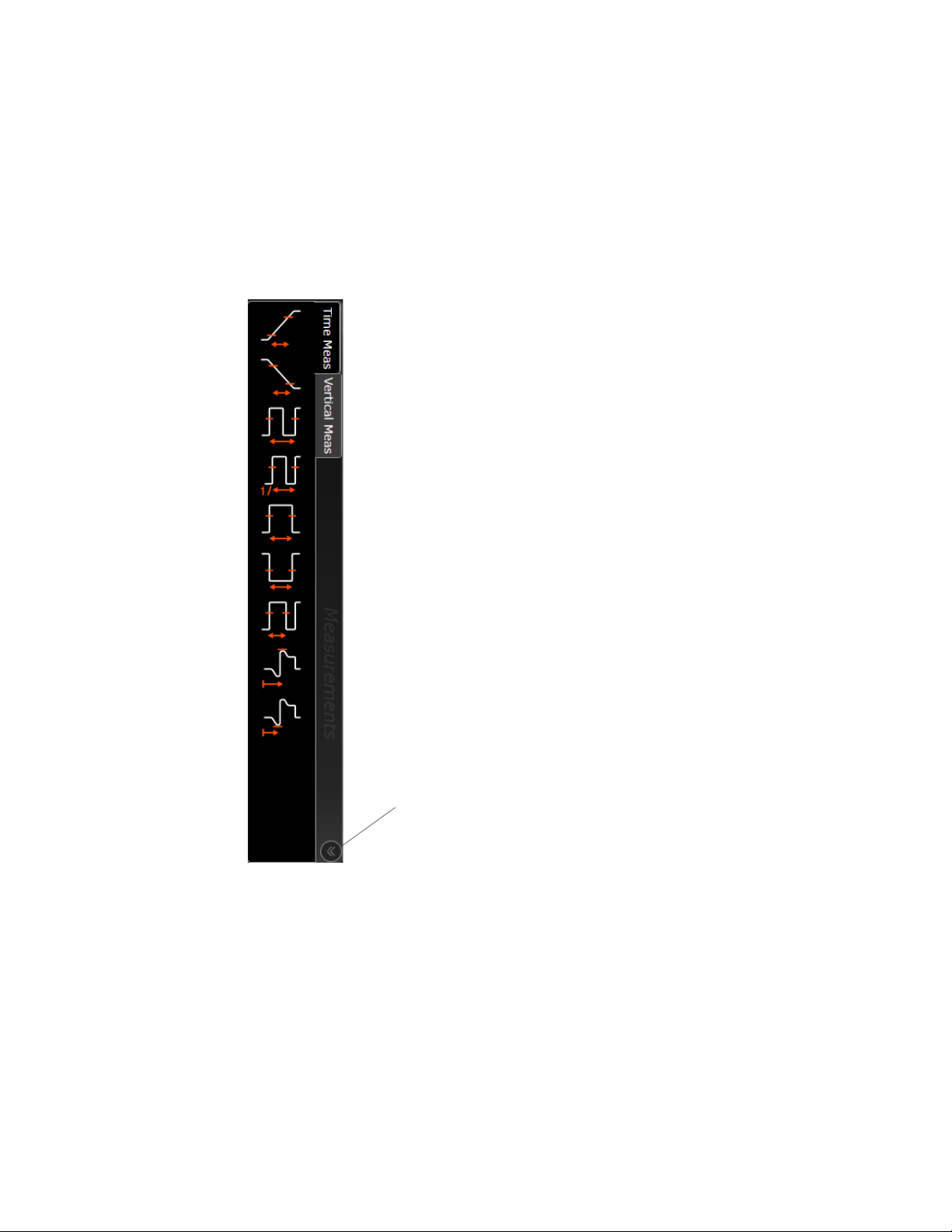
Making Measurements

To make a measurement, either drag a measurement icon to the waveform event you want to measure, or click a measurement icon and use the resulting dialog box to specify which source you want to measure.

Figure 21 Drag-and-drop measurements

For measurements on waveform features, such as those that involve waveform edges, if you click the measurement icon and specify a source, the measurement defaults to using the feature closest to the horizontal reference point. If you make the measurement using drag and drop, the measurement uses the waveform feature closest to the point where you drop the icon.

The most commonly used measurements are available in the drag-and-drop area. Others are available from the Add Measurement dialog box (Measure/Mark > Add Measurement...).

46 Keysight Infiniium MXR/EXR-Series Real-Time Oscilloscopes User's Guide

When you drag and drop a measurement icon on a waveform, the icon outline changes color to match the color of each waveform it touches so you can easily see which waveform will be measured.

For edge-sensitive measurements, a circled number appears in the waveform marker color when you drop the measurement icon on a waveform. This number shows exactly where the measurement is being made. It appears next to the measurement readout in the Results pane. This feature helps you distinguish measurement results from each other when you make multiple measurements on the same waveform but at different waveform features.

Using Quick Measurements

The default [Multi Purpose] key action is QuickMeas (see "[Multi Purpose] Key" on page 41). With this configuration:

• To turn on the quick measurement display, press [Multi Purpose]. The 10 preset measurements defined in the Quick Measurement configuration are enabled and results appear on the screen for the first waveform source.

Getting Started 2

• To measure parameters for another waveform, press [Multi Purpose] until that waveform is the one shown in the measurements window in the Results pane. Continuing to press [Multi Purpose] cycles through each of the waveforms available.

• To turn off the quick measurement display, cycle through all channels until the measurements are turned off.

See the Infiniium oscilloscope application's online help for information on how to configure the quick measurement capability. See "Accessing the Online Help" on page 51.

Keysight Infiniium MXR/EXR-Series Real-Time Oscilloscopes User's Guide 47

2 Getting Started

Enable or disable protocol decode

(currently not available)

Turn digital channels on or off

Using Digital Channels and Protocol Decode

On the front panel, just above the Vertical controls, are keys for digital channels and protocol decode.

Figure 22 Front panel [Digital] and [Protocol Decode] keys

Controlling Digital Channels

If your oscilloscope's MSO option is enabled, choose Setup > Digital Channels... to open the Digital dialog box so you can set up controls for the digital channels.

To turn the digital channels on, click the Add Waveforms button and select the

check box next to the , or press [Digital].

Decoding Serial Protocol Data

• To open the Protocol Decode dialog box so you can define parameters for selected decodes, choose Setup > Protocol Decode... or press [Protocol Decode].

You can perform up to four decodes at the same time using p1-p4.

• After selecting the protocol decode parameters, click Auto Setup to automatically configure the oscilloscope for the selected decode type.

• Decoded acquisition data appears in the Protocol Listing window.

48 Keysight Infiniium MXR/EXR-Series Real-Time Oscilloscopes User's Guide

Keysight Infiniium MXR/EXR-Series Real-Time Oscilloscopes

User's Guide

3 Demos and Online Help

Using the Demo Wizard / 50 Accessing the Online Help / 51

The graphical user interface has a Demo Wizard that illustrates many oscilloscope features and capabilities. There is also online help that describes oscilloscope features and capabilities in more detail.

3 Demos and Online Help

Using the Demo Wizard

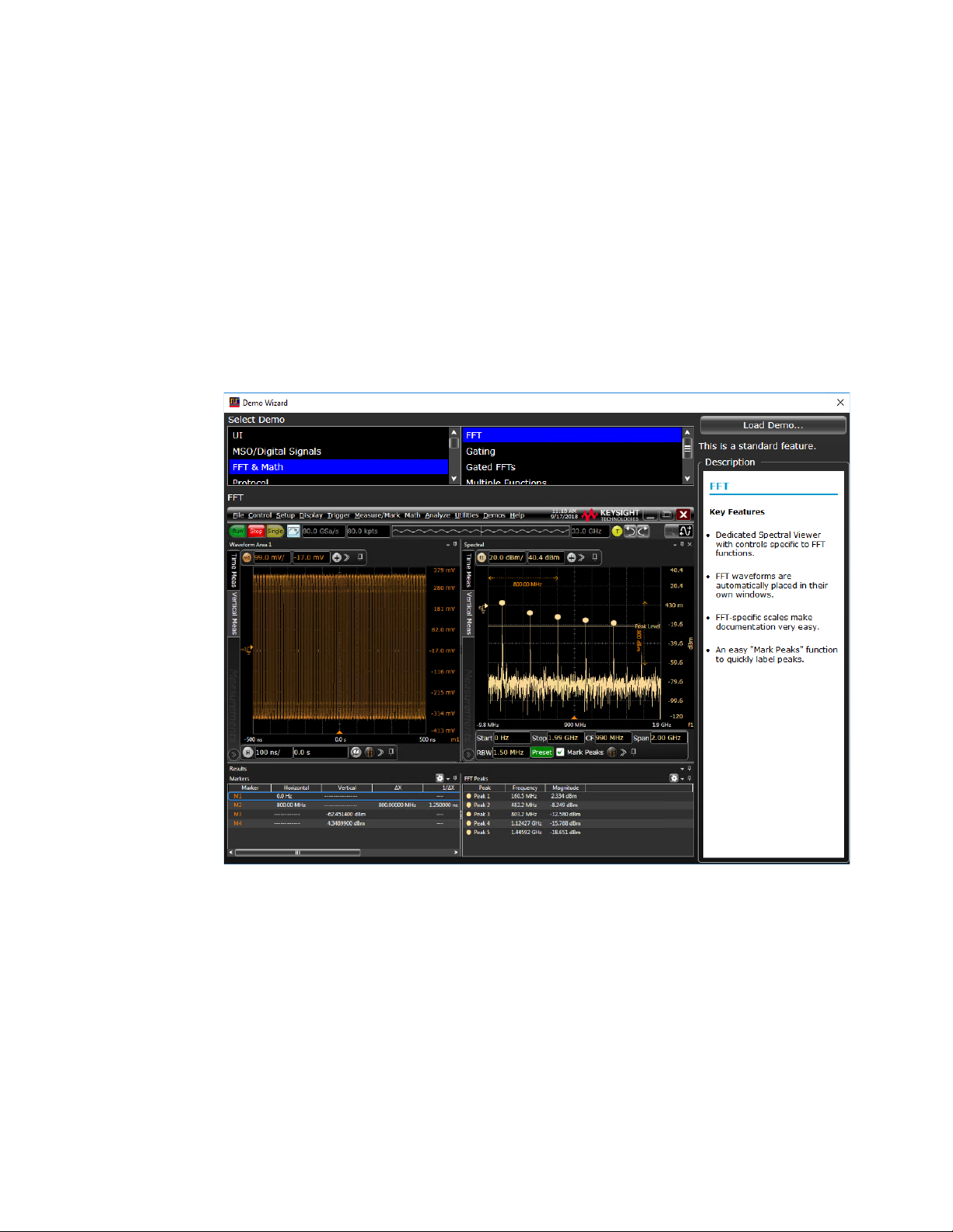
Your MXR/EXR-Series oscilloscope comes with a built-in demo wizard that showcases many Infiniium oscilloscope features. To see the demos, choose Demos > Tutorials & Demos... (or Help > Tutorials & Demos...). You can then select a specific demo, such as one for a particular protocol or one for a user interface showing bookmarks.

For example, the following screen display shows the initial demo page for the FFT

function. To experiment with the demo, click Load Demo....

Figure 23 FFT Demo

50 Keysight Infiniium MXR/EXR-Series Real-Time Oscilloscopes User's Guide

Accessing the Online Help

Displays the Help topic for this dialog box

There are two ways to access the online help:

• Click the question mark near the top right corner of a dialog box to open the help topic for that dialog box (Figure 24).

•Choose Help > Contents... from the main menu to open the online help home page (Figure 25).

Demos and Online Help 3

Figure 24 Help button for dialog box Help

Keysight Infiniium MXR/EXR-Series Real-Time Oscilloscopes User's Guide 51

3 Demos and Online Help

Figure 25 Online Help home page

There are several ways to find the information you need:

•Use the Search tab to search for a word or phrase. Use quotation marks to search for an exact phrase, such as "add waveform".

•Use the Contents tab to browse topics by double-clicking topics in the left pane.

•Use the Index tab to type in a keyword and search the index for that keyword, or scroll through the alphabetical list to find a topic.

•Use the Favorites tab to add preferred help topics to a list for easy reference.

For more details on using online help, click How to Use This Help under the Help and More Information topic in the Contents tab.

52 Keysight Infiniium MXR/EXR-Series Real-Time Oscilloscopes User's Guide

Keysight Infiniium MXR/EXR-Series Real-Time Oscilloscopes

User's Guide

4 Other Oscilloscope Tasks

Changing Windows Operating System Settings / 54 Installing Application Programs on Infiniium / 55 Forcing a Default Setup / 56 Hard Drive Recovery / 57 Cleaning the Oscilloscope / 58

This chapter describes tasks you may need to perform during ongoing use of the oscilloscope.

4 Other Oscilloscope Tasks

NOTE

Changing Windows Operating System Settings

Exit the oscilloscope application before changing any Windows operating system settings outside of the oscilloscope application.

Many Windows operating system settings can be changed to suit your own personal preferences. However, some operating system settings should not be changed because doing so would interfere with the proper operation of the oscilloscope.

• Do not change the Power Options.

• Do not change the Language settings.

• Do not remove Fonts.

• Do not change the screen resolution from 1920 by 1080 pixels.

• Do not use the Administrative Tools to enable or disable Internet Information Services (IIS) Manager. Use the Infiniium Remote Setup dialog box (Utilities > Remote...) to enable or disable the Web Server.

• Do not delete or modify the Infiniium Administrator user account.

54 Keysight Infiniium MXR/EXR-Series Real-Time Oscilloscopes User's Guide

Installing Application Programs on Infiniium

NOTE

CAUTION

The Infiniium oscilloscope has an open Windows operating system, which lets you install your own application software. Any application that runs on Microsoft Windows 10 and uses 16 GB of RAM or less may be installed on your Infiniium oscilloscope.

Exit the oscilloscope application before installing any software.

Installing an application that does not meet these requirements may break the oscilloscope application and require a hard drive recovery.

Other Oscilloscope Tasks 4

Keysight Infiniium MXR/EXR-Series Real-Time Oscilloscopes User's Guide 55

4 Other Oscilloscope Tasks

Forcing a Default Setup

If your Infiniium oscilloscope is not working properly when you start it up, follow these steps to perform a default setup and return the Infiniium to normal operation.

1 Choose Control > Default Setup or press [Default Setup]. 2 If the oscilloscope is still not working properly, choose Control > Factory Default

to return the oscilloscope to the default settings it had when it left the factory.

3 If the oscilloscope is still not working properly, turn it off.

4 Turn the oscilloscope back on. If it does not successfully restart, try recycling

the power again.

5 As soon as the Windows load screen disappears, press [Default Setup]. If the

oscilloscope still does not successfully restart, follow the instructions for recovering the hard drive. See "Hard Drive Recovery" on page 57.

56 Keysight Infiniium MXR/EXR-Series Real-Time Oscilloscopes User's Guide

Hard Drive Recovery

If you need to recover your Infiniium oscilloscope hard drive, follow these steps:

1 Back up your calibration and license files if they are still accessible:

a If the Infiniium application is available, launch the Keysight License Manager

(Utilities > Launch License Manager...) and capture a screen shot of the page. It lists the transportable and fixed perpetual licenses that Keysight will need to reissue.

b Copy the calibration folder (C:\ProgramData\Infiniium\cal) to an external

device, such as a flash drive.

c Copy the license file (C:\ProgramData\Infiniium\license.dat), which contains

legacy licenses, to an external device.

2 Turn off the oscilloscope.

3 Make sure a keyboard and mouse are connected to the USB host ports.

4 Turn on the oscilloscope and watch closely for the system prompts. As soon as

you see the prompt to choose Microsoft Windows or Instrument Image Recovery System, select Instrument Image Recovery System and follow the on-screen instructions.

Other Oscilloscope Tasks 4

5 Once the recovery process is finished and the oscilloscope is running, check in

the About Infiniium dialog box under installed options to see if all of the options you ordered are installed. If the options are not installed, install them using the license keys provided on the oscilloscope option license certificates you received, or refer to the back of the oscilloscope.

6 Restore the calibration folder and license files back to their original locations.

7 Restart the oscilloscope application to ensure the license.dat file reflects any

factory bandwidth licenses.

8 Send an email message to csg.support@keysight.com. Provide the License

Manager screen shot page you captured earlier, the oscilloscope's model and serial number from the rear panel of the scope, and the zip file you created earlier.

9 From the oscilloscope desktop, launch the Infiniium application. When the

application is active, perform an oscilloscope self-test (Utilities > Self Test...).

Keysight Infiniium MXR/EXR-Series Real-Time Oscilloscopes User's Guide 57

4 Other Oscilloscope Tasks

WARNING

CAUTION

WARNING

Cleaning the Oscilloscope

To prevent electrical shock, disconnect the Infiniium oscilloscope from mains before cleaning.

Clean the Infiniium oscilloscope with a soft dry cloth or one slightly dampened with a mild soap and water solution to clean the external case parts. Do not attempt to clean internally.

Do not use too much liquid in cleaning the oscilloscope. Water can enter the Infiniium oscilloscope panels, damaging sensitive electronic components.

To avoid electrostatic discharge (ESD), wear a grounded wrist strap when cleaning connectors.

Use alcohol to clean connectors. The power cord must be removed, and the oscilloscope must be in a well-ventilated area. Allow all residual alcohol moisture to evaporate, and the fumes to dissipate prior to powering up the oscilloscope. Dispose of the cleaning materials in a responsible manner.

58 Keysight Infiniium MXR/EXR-Series Real-Time Oscilloscopes User's Guide

Keysight Infiniium MXR/EXR-Series Real-Time Oscilloscopes

User's Guide

5 Calibrating the Oscilloscope

When to Perform a User Calibration / 60 Equipment Required / 61 Calibration Time / 62 Calibration Procedure / 63

A calibration is simply an oscilloscope self-adjustment. The purpose of a calibration is performance optimization.

There are two ways to calibrate an Infiniium MXR/EXR-Series oscilloscope:

•A user calibration, also known as a self calibration, includes the minimum set of calibrations and is intended to be run by oscilloscope users. It can include a time scale calibration.

•A service calibration is performed only by Keysight Service Center technicians.

This chapter describes how to run a user (self) calibration.

5 Calibrating the Oscilloscope

When to Perform a User Calibration

When to perform a user calibration:

• Standard calibration only—When the oscilloscope's operating temperature (after the 30-minute warm-up period) is more than ±5 °C different from that of the last calibration. Be sure to perform a standard user calibration (do not perform the time scale cal)—even if one was recently performed—when environmental temperature conditions cause the oscilloscope's operating temperature to change, such as when the oscilloscope is moved to a test rack or chamber.

• Standard and time scale cal—When it has been more than 1 year since the last time scale calibration, or when you replace the acquisition board.

60 Keysight Infiniium MXR/EXR-Series Real-Time Oscilloscopes User's Guide

Equipment Required

Equipment Critical specifications Recommended part number

Calibrating the Oscilloscope 5

50 Ω BNC Cable 50 Ω characteristic impedance

BNC cable

10 MHz Signal Source (required for time scale calibration)

Frequency accuracy better than ±41 ppb

54609-61609

53220A with Opt. 010

Keysight Infiniium MXR/EXR-Series Real-Time Oscilloscopes User's Guide 61

5 Calibrating the Oscilloscope

Calibration Time

It takes approximately 70 minutes to run the user calibration on the oscilloscope, including the time required to change cables from channel to channel.

62 Keysight Infiniium MXR/EXR-Series Real-Time Oscilloscopes User's Guide

Calibration Procedure

NOTE

CAUTION

Clear this

Performing a user calibration will invalidate the oscilloscope's Certificate of Calibration. If NIST (National Institute of Standards and Technology) traceability is required, perform the procedures in Chapter 6, “Testing Performance,” starting on page 65 using traceable sources.

1 Let the oscilloscope warm up before running the calibration.

The oscilloscope must be warmed up (with the oscilloscope application running) for at least 30 minutes at ambient temperature before starting the calibration procedure. Failure to allow warm up may result in inaccurate calibration.

2 Click Utilities > Calibration....

3 Clear the Cal Memory Protect check box.

Calibrating the Oscilloscope 5

You cannot run a user calibration if this check box is selected. See the following figure.

4 Click Start Frame Cal; then, follow the instructions on the screen.

The routine will prompt you to follow these steps:

a Disconnect everything from all inputs and Aux Out.

b Select the level of calibration you want to perform.

Keysight Infiniium MXR/EXR-Series Real-Time Oscilloscopes User's Guide 63

5 Calibrating the Oscilloscope

NOTE

When performing the time scale calibration using the 53220A-010 universal frequency counter/timer, the precision 10 MHz reference is available from the Int Ref Out connector on the rear panel of the 53220A counter/timer.

• Standard Calibration — Time scale calibration will not be performed. Time

scale calibration factors from the previous time scale calibration will be used and the 10 MHz reference signal will not be required. The remaining calibration procedure will continue.

• Standard Calibration and Time Scale Calibration—Time scale calibration

will be performed. This option requires you to connect a 10 MHz reference signal to channel 1 that meets the following specifications. Failure to use a reference signal that meets these specifications will result in an inaccurate calibration.

• Frequency: 10 MHz, max ±41 ppb = 10 MHz, max ±0.41 Hz

• Amplitude: 0.2 V peak-to-peak to 5.0 V peak-to-peak

• Wave shape: Sine or Square

c Connect the 50 Ω BNC cable from Aux Out to each of the channel inputs as

requested.

d Connect the 50 Ω BNC cable to Aux Trig In as requested.

e Follow the directions for calibrating the digital channels (models with MSO

option).

f A Passed/Failed indication is displayed for each calibration section.

If any section has failed, wait until the calibration is complete and then select the Enable Details check box for information on the failures. Also check the cable connections.

5 When the calibration procedure is complete, click Close.

64 Keysight Infiniium MXR/EXR-Series Real-Time Oscilloscopes User's Guide

Keysight Infiniium MXR/EXR-Series Real-Time Oscilloscopes

User's Guide

6 Testing Performance

Performance Verification General Information / 66 Input Impedance Test / 67 Offset Accuracy Test / 69 DC Gain Accuracy Test / 76 Analog Bandwidth—Maximum Frequency Test / 79 Time Scale Accuracy (TSA) Test / 86 Performance Test Record / 89

Full performance verification for the MXR/EXR-Series oscilloscopes consists of three main procedures:

1 Performing the internal oscilloscope self-tests to ensure that the measurement

system is functioning properly. To perform the self-tests, click Utilities > Self

Test.... Then select Scope SelfTest from the Available Self Test drop-down list

box, click Start, and follow the on-screen instructions. If any of the self tests fail, ensure that the failure is diagnosed and repaired before calibrating and testing performance.

2 Calibrating the oscilloscope, as described in Chapter 5, “Calibrating the

Oscilloscope,” starting on page 59.

3 Testing the oscilloscope to ensure that it is performing to specification. This

chapter describes these performance test procedures.

6 Testing Performance

Performance Verification General Information

Performance Test Interval

The procedures in this section may be performed for incoming inspection and should be performed periodically to verify that the oscilloscope is operating within specification. The recommended test interval is once per year or after 2000 hours of operation. Performance should also be tested after repairs or major upgrades.

Performance Test Record

A test record form is provided at the end of this section. This record lists performance tests and test limits, and provides space to record test results.

Test Order

The tests in this section may be performed in any order. However, we recommend conducting the tests in the order presented, as the order represents an incremental approach to performance verification. This approach may be useful when you are troubleshooting a suspected problem.

Test Equipment

Lists of equipment needed to conduct each test are provided for each test procedure. The procedures are written to minimize the number and types of test equipment and accessories required. The test equipment in these lists are currently available for sale by Keysight at the time this document was written. In some cases, the test procedures use features specific to the test equipment in the recommended equipment list. However, other equipment, cables, and accessories that satisfy the critical specifications in these lists may be substituted for the recommended models with some modification to the test procedures.

Contact Keysight Technologies for more information about the Keysight products in these lists.

66 Keysight Infiniium MXR/EXR-Series Real-Time Oscilloscopes User's Guide

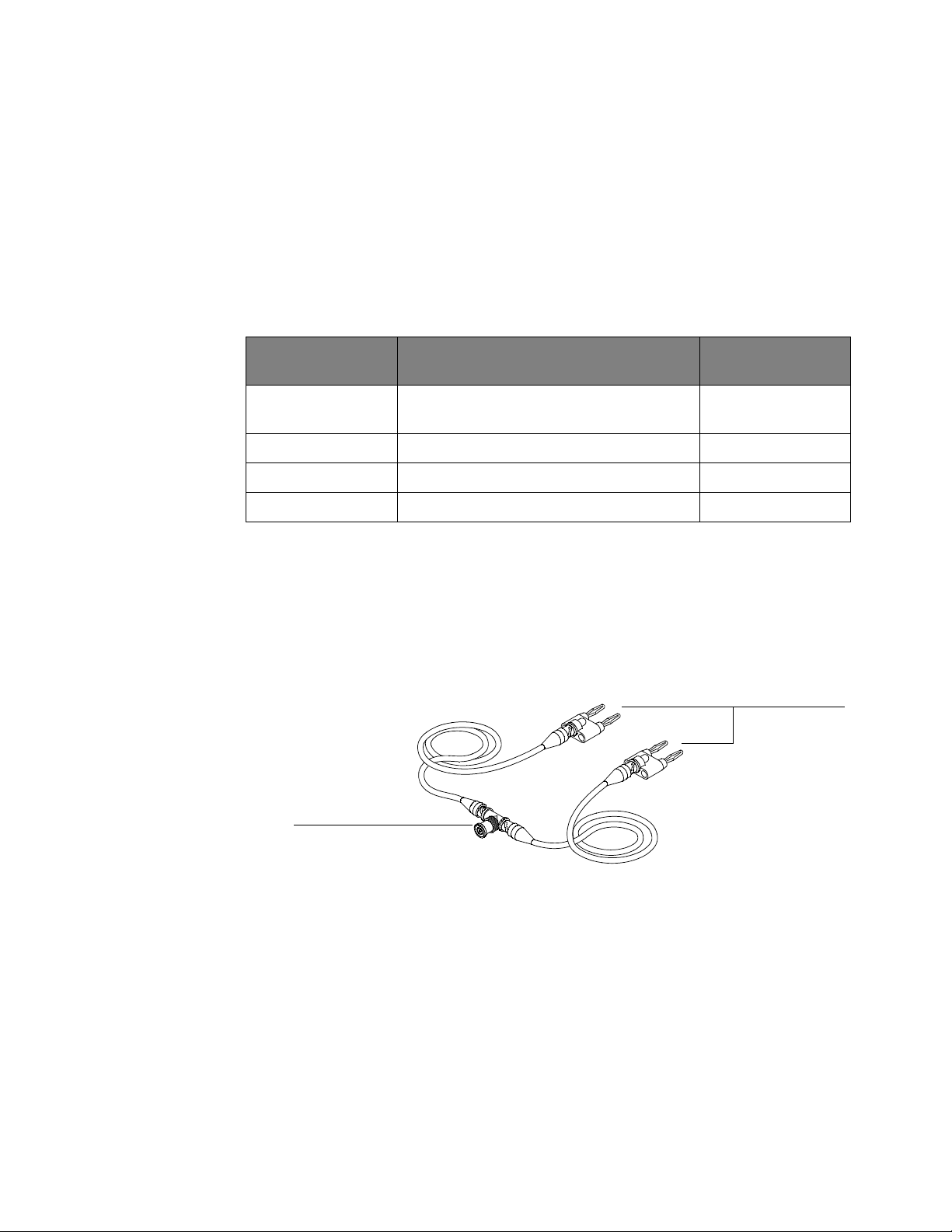
Input Impedance Test

To DMM 4-wire inputs

To oscilloscope channel input

This test checks the input impedance of the vertical inputs. A four-wire measurement is used to accurately measure the 50 Ω and 1 MΩ inputs.

Specifications •1MΩ ±1%

•50Ω ±3.5%

Equipment

Required

Description Critical specifications Recommended model

Testing Performance 6

or part number

Procedure

Digital Multimeter Measure resistance (4-wire) at better than

±0.1% accuracy

Cables (2) BNC 10503A

Adapter BNC Tee (m)(f)(f) 1250-0781

Adapters (2) BNC (f) to dual banana (m) 1251-2277

1 Set up the multimeter to make a four-wire resistance measurement.

2 Assemble the test cables:

a Use the two BNC-to-banana adapters to connect one end of each BNC

34411A, 3458A, or 34465A

cable to the four-wire resistance connections on the multimeter.

b Connect the free ends of the cables to the BNC tee as shown here.

3 Connect the male end of the BNC tee to the channel 1 input of the

oscilloscope.

4 Click Control > Factory Default to set the oscilloscope to default conditions. 5 Open the Channel dialog box for channel 1 (Setup > Channel 1...). Set the scale to

5 mV/div and set the channel input impedance to 50 Ω. Verify a resistance reading of 50 Ω ±1.75 Ω.

6 Record the readings in the "Input Impedance Test" table of the "Performance

Test Re cord" on page 89.

7 Repeat step 5 and step 6 for the remaining 50 Ω vertical scale settings in

Table 6.

Keysight Infiniium MXR/EXR-Series Real-Time Oscilloscopes User's Guide 67

6 Testing Performance

NOTE

8 Repeat step 3 through step 7 on the remaining channels of the oscilloscope.

9 Repeat step 3 through step 8 using an input resistance of 1 MΩ instead of 50 Ω

and verify resistance readings of 1 MΩ ±10 kΩ.

Due to the current source limitations of the 34411A/3458A/34465A DMM, be sure to set it to 10 MΩ range instead of Auto Range when testing the 1 MΩ resistance.

68 Keysight Infiniium MXR/EXR-Series Real-Time Oscilloscopes User's Guide

Offset Accuracy Test

CAUTION

NOTE

Ensure that the input voltage to the oscilloscope never exceeds ±5 V.

The oscilloscope must be warmed up (with the oscilloscope application running) for at least 30 minutes at ambient temperature prior to the start of any performance test.

Specifications

Offset Accuracy ±0.1 div ±2 mV ±1.0% of offset setting for offsets < 2V

50 Ω Input Impedance: Full scale is defined as 8 vertical divisions. Magnification is used below 2 mV/div. Below 2 mV full scale is defined as 16 mV. The major scale settings are 5 mV, 10 mV, 20 mV, 50 mV, 100 mV, 200 mV, 500 mV and 1 V.

1MΩ Input Impedance: Full scale is defined as 8 vertical divisions. The major scale settings are 5 mV, 10 mV, 20 mV, 50 mV, 100 mV, 200 mV, 500 mV, 1 V, 2 V, and 5 V.

Testing Performance 6

±0.1 div ±2 mV ±1.5% of offset setting for offsets ≥ 2V

Equipment

Required

Procedure

Description Critical specifications Recommended model

or part number

Digital Multimeter DC voltage measurement accuracy better than

±0.1% of reading

Cable Assembly (2 required)

DC Power Supply 40 V 6614C

Adapter BNC Tee (m)(f)(f) 1250-0781

Adapters (2) BNC (f) to dual banana (m) 1251-2277

1 Disconnect all cables from the oscilloscope channel inputs. 2 Click Control > Factory Default. The input impedance for channel 1 should be

50 Ω characteristic impedance, BNC (m) connectors

34411A, 3458A, or 34465A

8120-1840

50 Ω.

3 Click Setup > Acquisition.... In the Acquisition dialog box, enable averaging and

set # of Averages to 256.

Keysight Infiniium MXR/EXR-Series Real-Time Oscilloscopes User's Guide 69

6 Testing Performance

4 Configure the oscilloscope to measure the average voltage (V avg) on channel

1 as follows:

a Change the vertical scale of channel 1 to 5 mV/div.

b Click the Vertical Meas tab on the left side of the screen, then drag and drop

the Average measurement icon onto the channel 1 waveform.

70 Keysight Infiniium MXR/EXR-Series Real-Time Oscilloscopes User's Guide

Testing Performance 6

NOTE

5 Press [Clear Display] on the oscilloscope and wait for the number of averages

display (top right area of screen) to return to 256. Record the oscilloscope's mean V avg reading in the Vzero-error column of Table 8 of the Performance Test Record. Use the Channel dialog box to select 1 MΩ impedance and then repeat step 3 to step 5. Record the reading in Table 9 for channel 1.

• For all oscilloscope readings in this procedure, use the mean value in the Measurement Results

pane at the bottom of the screen.

• If a question mark appears in front of any values in the Results pane, press [Clear Display] on the

oscilloscope, wait for the number of averages to return to 256, and then record the oscilloscope reading. The question mark indicates that the oscilloscope could not make a reliable measurement.

Keysight Infiniium MXR/EXR-Series Real-Time Oscilloscopes User's Guide 71

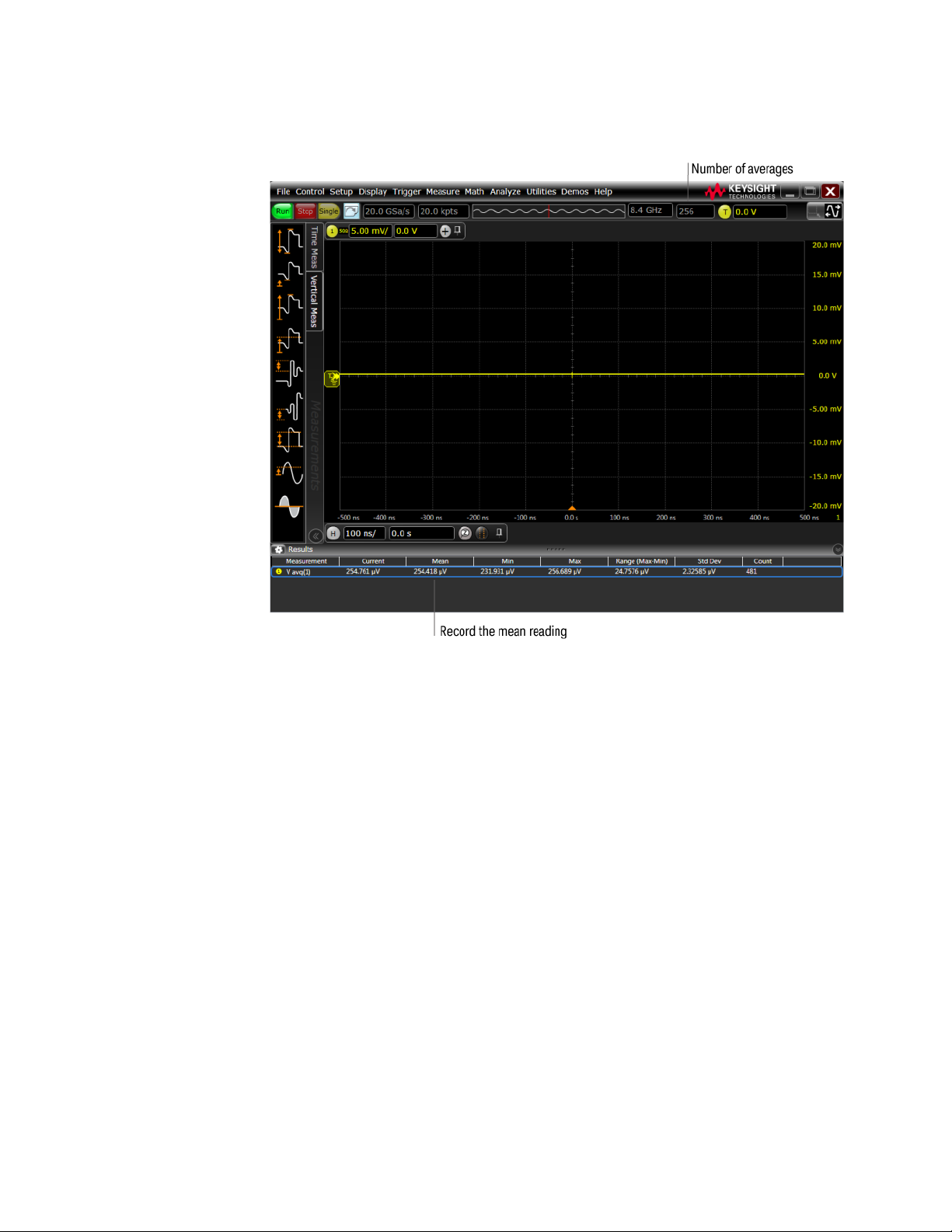
6 Testing Performance

6 Change the vertical scale of channel 1 to 10 mV/div, press [Clear Display], wait

for the number of averages to return to 256, and then record the oscilloscope's mean V avg reading in the Vzero-error column of Table 8. Use the Channel dialog box to select 1 MΩ impedance and repeat for 1 MΩ. Record the results in

Table 9.

7 Repeat step 6 for the remaining vertical scale settings for channel 1 in Table 8

and in Table 9 of the Performance Test Record.

8 Click Control > Factory Default, turn off channel 1, and turn the channel 2 display

on.

9 Configure the oscilloscope to measure V avg on channel 2 as follows:

a In the Acquisition dialog box, enable averaging and set # of Averages to 256.

b Change the vertical scale of channel 2 to 5 mV/div.

c Drag and drop the Average voltage measurement icon onto the channel 2

waveform.

10 Press [Clear Display] on the oscilloscope, wait for the number of averages to

return to 256, and then record the oscilloscope's mean V avg reading in the Vzero-error column of Table 8. Use the Channel dialog box to select 1 MΩ impedance and repeat for 1 MΩ. Record the results in Table 9.

72 Keysight Infiniium MXR/EXR-Series Real-Time Oscilloscopes User's Guide

Testing Performance 6

Channel Input on MXR-Series Oscilloscope

BNC (f) to dual banana

(1251-2277)

6614C DC Supply

NOTE

11 Repeat step 9b and step 10 for the remaining vertical scale settings for channel

12 Repeat step 8 through step 11 for the remaining channels.

13 Ensure that each Vzero-error is less than the corresponding Vzero-error Limit

entry in the Offset Accuracy Test table.

14 Make the connections to oscilloscope channel 1 as shown below.

• Where the BNC Tee adapter is used, it is important to connect it directly to the oscilloscope

channel input to minimize ground potential differences and to ensure that the DMM measures the input voltage to the oscilloscope channel as accurately as possible. Differences in ground potential can be a significant source of measurement error, particularly at high scope sensitivities.

• It also helps to reduce ground potential differences if the oscilloscope and DMM are connected to

the same AC supply circuit.

• 256 averages are used in the oscilloscope measurements of this section to reduce measurement

noise and to reduce the measurement error due to resolution.

15 Set up the DMM to perform DC voltage measurements. 16 Click Control > Factory Default to default to channel 1.

17 Configure the oscilloscope to measure the average voltage on channel 1 as

follows:

a Click Setup > Acquisition.... In the Acquisition dialog box, enable averaging

and set # of Averages to 256.

b Change the vertical scale of the channel under test to 5 mV/div.

c Drag and drop the Average voltage measurement icon onto the channel 1

waveform.

Keysight Infiniium MXR/EXR-Series Real-Time Oscilloscopes User's Guide 73

6 Testing Performance

18 Using the Channel dialog box, set the channel's offset value to 60.0 mV and the

impedance to 50 Ω (or to an offset of 2 V and the impedance to 1 MΩ if this is your second pass through this test and you are using the 1 MΩ input impedance version).

19 Set the DC supply voltage (External Supply Setting) to +60.0 mV (or +2 V for

the 1 MΩ version of this test).

20 Press [Clear Display] on the oscilloscope, wait for the number of averages to

return to 256, and then record the DMM voltage reading as VDMM+ and the scope V avg reading as VScope+ in either Table 8 or Table 9 (depending on which version of the test you are on). Fill in the Verror+ column by using the following equation:

Verror+ = VDMM+ - Vscope+

Verror+ must be within the limits specified by the corresponding Offset Accuracy Limit listed in the table.

21 Change the channel 1 offset value to -60.0 mV (or -2 V for the 1 MΩ version of

this test).

22 Set the DC supply voltage to -60.0 mV (or -2 V for the 1 MΩ version of this

test).

23 Press [Clear Display] on the oscilloscope, wait for the number of averages to

return to 256, and then record the DMM voltage reading as VDMM- and the scope V avg reading as VScope- in either Table 8 or Table 9 (depending on

74 Keysight Infiniium MXR/EXR-Series Real-Time Oscilloscopes User's Guide

Testing Performance 6

which version of the test you are on). Fill in the Verror- column by using the following equation:

Verror- = VDMM- - Vscope-

Verror- must be within the limits specified by the corresponding Offset Accuracy Limit listed in the table.

24 Repeat step 17b and step 18 to step 23 for the remaining channel 1 vertical

scale settings in Table 8 or Table 9 (depending on which version of the test you are performing). For each measurement, set both the DC supply voltage (External Supply Setting) and the Channel offset voltage to the positive External Supply Setting value and then to the negative External Supply Setting value in the External Supply Setting column of the Offset Accuracy Test table for each of the vertical scale settings.

25 Move the Tee connector to the next channel input and repeat step 17 to step 24

for the remaining channels.

26 Repeat step 16 through step 25 for the 1 MΩ channel input impedance setting.

This means you should follow the directions exactly as stated except in step 18 you will select the 1 MΩ button instead of the 50 Ω one and all values will be entered in Table 9 of the Performance Test Record rather than Table 8. Also be sure to use the external supply settings and offset values from the 1 MΩ version of the Offset Accuracy Test table as they are different than the 50 Ω version.

Keysight Infiniium MXR/EXR-Series Real-Time Oscilloscopes User's Guide 75

6 Testing Performance

CAUTION

NOTE

DC Gain Accuracy Test

Ensure that the input voltage to the oscilloscope never exceeds ±5 V.

The oscilloscope must be warmed up (with the oscilloscope application running) for at least 30 minutes at ambient temperature prior to the start of any performance test.

Specifications

DC Gain Accuracy

1MΩ Input Impedance: Full scale is defined as 8 vertical divisions. The major scale settings are 5 mV, 10 mV, 20 mV, 50 mV, 100 mV, 200 mV, 500 mV, 1 V, 2 V, and 5 V.

±2% of full scale at full resolution channel scale (±5 °C from calibration temperature)

Equipment

Required

Description Critical specifications Recommended model

or part number

Digital Multimeter DC voltage measurement accuracy better than

±0.1% of reading

Cable Assembly (2 required)

DC Power Supply 40 V 6614C

Adapter BNC Tee (m)(f)(f) 1250-0781

Adapters (2) BNC (f) to dual banana (m) 1251-2277

50 Ω characteristic impedance, BNC (m) connectors

34411A, 3458A, or 34465A

8120-1840

76 Keysight Infiniium MXR/EXR-Series Real-Time Oscilloscopes User's Guide

Testing Performance 6

Channel Input on MXR-Series Oscilloscope

BNC (f) to dual banana

(1251-2277)

6614C DC Supply

NOTE

Procedure 1 Make the connections to oscilloscope channel 1 as shown below.

• Where the BNC Tee adapter is used, it is important to connect it directly to the oscilloscope

• It also helps to reduce ground potential differences if the oscilloscope and DMM are connected to

the same AC supply circuit.

• 256 averages are used in the oscilloscope measurements of this section to reduce measurement

noise and to reduce the measurement error due to resolution.

2 Click Control > Factory Default, then configure the oscilloscope as follows:

a Click Setup > Acquisition....

b In the Acquisition dialog box, enable averaging and set # of Averages to 256.

3 Set the DC Supply voltage (External Supply Setting) to +15 mV.

4 Use the Channel dialog box to set the channel 1 vertical scale to 5 mV/div, and

make sure the input impedance is set to 50 Ω.

5 Drag and drop the Average voltage measurement icon onto the channel 1

waveform.

6 Press [Clear Display] on the oscilloscope, wait for the number of averages to

return to 256, and then record the DMM voltage reading as VDMM+ and the scope mean V avg reading as VScope+ in Table 10 of the Performance Test Record.

7 Change the DC Supply voltage to -15 mV. 8 Press [Clear Display] on the oscilloscope, wait for the number of averages to

return to 256, and then record the DMM voltage reading (VDMM- column) and

Keysight Infiniium MXR/EXR-Series Real-Time Oscilloscopes User's Guide 77

6 Testing Performance

the scope V avg reading (Vscope- column) in Table 10 of the Performance Test Record.

9 Repeat step 8 for the remaining vertical scale settings for channel 1 shown in

Table 10 of the Performance Test Record.

10 Click Control > Factory Default, turn off channel 1 and turn the channel 2 display

on.

11 Set the DC Supply voltage (External Supply Setting) to +15 mV.

12 Configure the oscilloscope to measure the average voltage on channel 2:

a Click Setup > Acquisition.... In the Acquisition dialog box, enable averaging

and set # of Averages to 256.

b Change the vertical scale of channel 2 to 5 mV/div.

c Drag and drop the Average voltage measurement icon onto the channel 2

waveform.

13 Press [Clear Display] on the oscilloscope, wait for the number of averages to

return to 256, and then record the DMM voltage reading (VDMM+) and the scope V avg reading (VScope+) in Table 10 of the Performance Test Record.

14 Repeat step 13 for the remaining vertical scale settings for channel 2 in

Table 10 of the Performance Test Record.

15 Repeat step 10 through step 14 for the remaining channels.

16 Repeat step 2 through step 15 using 1 MΩ for the scope input impedance

rather than 50 Ω. The steps should be followed exactly except in step 4, you should select the 1 MΩ button from the Impedance section of the Channel dialog box rather than 50 Ω and all values should be entered in Table 11 rather than Table 10.

17 Calculate the offset gains for the 50 Ω test and the 1 MΩ test using the

following expression and record these values in Table 10 and Table 11 of the Performance Test Record.

78 Keysight Infiniium MXR/EXR-Series Real-Time Oscilloscopes User's Guide

Analog Bandwidth—Maximum Frequency Test

CAUTION

NOTE

Ensure that the input voltage to the oscilloscope never exceeds ±5 V.

The oscilloscope must be warmed up (with the oscilloscope application running) for at least 30 minutes at ambient temperature prior to the start of any performance test.

Specifications

Analog Bandwidth (-3 dB)

MXR608A, MXR604A 6 GHz

MXR408A, MXR404A 4 GHz

Testing Performance 6

MXR258A, MXR254A, EXR258A, EXR254A 2.5 GHz

MXR208A, MXR204A, EXR208A, EXR204A 2 GHz

MXR108A, MXR104A, EXR108A, EXR104A 1 GHz

MXR058A, MXR054A, EXR058A, EXR054A 500 MHz

Keysight Infiniium MXR/EXR-Series Real-Time Oscilloscopes User's Guide 79

6 Testing Performance

Power meter N1912A

Power sensor cable

Power splitter 11667B

Power sensor E4413A

SMA to BNC adapter

N-type to 3.5 mm SMA adapter (part not shown)

Coaxi al cable

Microwave CW Generator E8257D

MXR-Series oscilloscope channel input

Equipment

Required

Description Critical specifications Recommended model

or part number

Microwave CW Generator

Power Sensor Cable N1912-61020

Power Splitter 2 Resistor Power Splitter (f)

Power Meter Keysight P-series with power sensor

Power Sensor Maximum Frequency ≥ 14 GHz

Coaxial Cable 50 Ω Characteristic Impedance

N-Type to SMA Adapter

SMA to BNC Adapter SMA (m) to Precision BNC (No Substitute) 1250-1200

Maximum Frequency ≥ 14 GHz

Power range: -20 dBm to +16 dBm into 50 Ω

Output resistance = 50 Ω

Max Frequency ≥18 GHz

compatibility

Power range: -24 dBm to +16 dBm

3.5 mm (m) to 3.5 mm (m) SMA connectors Max Frequency ≥ 8 GHz

N-type to 3.5 mm (m) SMA 1250-1750

E8257D with Opt 520

11667B

N1912A

E4413A

8120-4948

Connections

80 Keysight Infiniium MXR/EXR-Series Real-Time Oscilloscopes User's Guide

NOTE

• Connect output 1 of the 11667B splitter to the oscilloscope Channel n input directly using the

1250-1200 adapter, without any additional cabling or adapters.

• Connect output 2 of the 11667B power splitter to the power sensor using the 1250-1750 N-type to

3.5 mm adapter, without any additional cabling or adapters.

• Minimize the use of other adapters.

• Ensure that SMA and 3.5 mm connectors are tightened properly:

8 in-lbs (90 N-cm) for 3.5 mm

5 in-lbs (56 N-cm) for SMA

Procedure 1 Preset the power meter.

2 Ensure that the power sensor is disconnected from any source and zero the

meter.

3 Connect the power sensor to the power meter's Power Ref connector and

calibrate the meter.

4 Make the connections to oscilloscope channel 1 as shown in the preceding

connection diagram.

Testing Performance 6

5 Set up the power meter to display measurements in units of Watts. 6 Click Control > Factory Default, then configure the oscilloscope as follows:

a Ensure the channel under test is displayed and all other channels are turned

off.

b In the Channel dialog box, set the vertical scale of the channel under test to

5 mV/div and the input impedance to 50 Ohms.

c Set the horizontal scale to 16 ns/div (to display 8 cycles of a 50 MHz

waveform).

d Click Setup > Acquisition... and ensure the acquisition parameters are set up

as follows:

• Sin(x)/x Interpolation = Auto

• Analog Averaging = Enabled with # of Averages set to 16

• Analog Memory Depth = Automatic

• Analog Sampling rate = Maximum (select the Manual button and click

the up-arrow as high as it goes)

e Click Measure > Add Measurement....

f In the Add Measurement dialog box, click Vertical and RMS, and configure

the measurement as follows:

• Source = Channel 1

• Measurement Area = Entire Display

• RMS Type = AC

Keysight Infiniium MXR/EXR-Series Real-Time Oscilloscopes User's Guide 81

6 Testing Performance

NOTE

7 Set the generator to apply a 50 MHz sine wave with a peak-to-peak amplitude

of about four divisions.

Use the following table to determine the approximate required signal amplitude.

The amplitude values in the table are not absolutely required. If your generator is unable to produce the recommended amplitude, then set the generator to the highest value that does not produce a vertically clipped signal on the oscilloscope.

Table 5 Nominal Generator Amplitude Settings

Oscilloscope Vertical Scale Generator Signal Amplitude

(Vp-p)

5 mV/div 0.02 -30

10 mV/div 0.04 -24

20 mV/div 0.08 -18

50 mV/div 0.20 -10

100 mV/div 0.40 -4

200 mV/div 0.80 +2

500 mV/div 2.0 +10

1V/div 4.0 +16

8 Measure the input power to the oscilloscope channel and convert this

Generator Signal Amplitude (dBm)

measurement to Volts RMS using the expression:

For example, if the power meter reading is 4.0 μW, then Vin = (4.0*10-6 * 50 Ω)1/2 = 14.1 mVrms.

Record the RMS voltage in Table 12 of the Performance Test Record (in the Vin @ 50 MHz column).

9 Press [Clear Display] on the oscilloscope and record the scope V rms reading in

Table 12 of the Performance Test Record (Vout @ 50 MHz column).

• For all oscilloscope readings in this procedure, use the mean value in the Measurement Results

area at the bottom of the screen.

• If a question mark appears in front of any value at the bottom of the screen, press [Clear Display]

on the oscilloscope, wait for the number of averages to return to 16, and then record the oscilloscope reading.

82 Keysight Infiniium MXR/EXR-Series Real-Time Oscilloscopes User's Guide

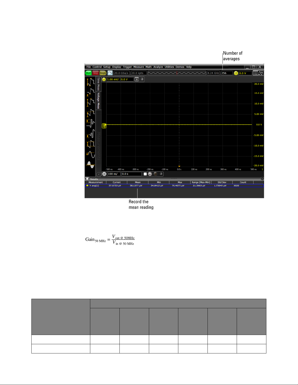
Testing Performance 6

10 Calculate the reference gain as follows:

Record this value in the Calculated Gain @50 MHz column in Table 12 of the Performance Test Record.

11 Change the generator frequency to the maximum value for the model being

tested as shown in the table below. It is not necessary to adjust the signal amplitude at this point in the procedure.

Setting Model

MXR608A, MXR604A

Maximum Frequency 6 GHz 4 GHz 2.5 GHz 2 GHz 1 GHz 500 MHz

MXR408A, MXR404A

MXR258A, MXR254A, EXR258A, EXR254A

MXR208A, MXR204A, EXR208A, EXR204A

MXR108A, MXR104A, EXR108A, EXR104A

MXR058A, MXR054A, EXR058A, EXR054A

Scope Horizontal Scale 150 ps/div 200 ps/div 320 ps/div 400 ps/div 800 ps/div 1.6 ns/div

Keysight Infiniium MXR/EXR-Series Real-Time Oscilloscopes User's Guide 83

6 Testing Performance

12 Change the oscilloscope horizontal scale to the value for the model under test

in the preceding table.

13 Measure the input power to the oscilloscope channel at the maximum

frequency and convert this measurement to Volts RMS using the expression:

For example, if the power meter reading is 4.0 μW, then Vin = (4.0*10-6 * 50 Ω)1/2 = 14.1 mVrms.

Record the RMS voltage in Table 12 of the Performance Test Record (Vin @ Max Freq column).

14 Press [Clear Display] on the oscilloscope and record the scope V rms reading in

Table 12 of the Performance Test Record (Vout @ Max Freq column).

15 Calculate the gain at the maximum frequency using the expression:

For example, if (Vout @ Max Frequency) = 13.825 mV, (Vin @ Max Frequency) =

13.461 mV and Gain @ 50MHz = 1.0023, then:

Record this value in the Calculated Gain @Max Freq column in Table 12 of the Performance Test Record. To pass this test, this value must be greater than

-3.0 dB.

16 Change the scope setup as follows:

a Change the channel vertical scale to 10 mV/div.

b Reset the horizontal scale to 16 ns/div (to display 8 cycles of a 50 MHz

waveform).

17 Change the generator output as follows:

a Reset the generator frequency to 50 MHz.

b Change the amplitude to the value suggested for this scale setting in the

Nominal Generator Amplitude Settings table.

18 Repeat step 8, step 9, and step 10 to measure the reference gain at 50 MHz for

this scale.

19 Repeat step 11 through step 15 to measure the gain at maximum frequency for

this scale setting.

84 Keysight Infiniium MXR/EXR-Series Real-Time Oscilloscopes User's Guide

Testing Performance 6

20 Repeat step 15 through step 19 to complete measuring gains for remaining

scale settings for channel 1 in Table 12 of the Performance Test Record.

21 For each of the remaining channels, move the splitter to the channel under test

and change the oscilloscope configuration as follows:

a Click Control > Factory Default.

b Ensure the channel under test is displayed and all other channels are turned

off.

c Set the vertical scale of the channel to 5 mV/div.

d Set the horizontal scale to 16 ns/div (to display 8 cycles of a 50 MHz

waveform).

e Click Trigger> Setup Trigger... and change the source to the channel.

f Click Measure > Add Measurement.... Select the Vertical RMS voltage

measurement, the channel under test as the source, Entire Display as the Measurement Area, and AC for the RMS Type.

g Repeat step 6d and step 7 to step 20 to complete measuring gains for the

channel.

Keysight Infiniium MXR/EXR-Series Real-Time Oscilloscopes User's Guide 85

6 Testing Performance

NOTE

Time Scale Accuracy (TSA) Test

This procedure verifies the maximum TSA specification for the oscilloscope.

Description TSA refers to the absolute accuracy of an oscilloscope's time scale. Because TSA

depends directly on frequency of a crystal oscillator, it is comprised of two components: an initial setting accuracy component and an aging component.

The initial setting accuracy component applies to the oscilloscope's 10 MHz OCXO frequency accuracy immediately after a calibration, whether performed at the factory, by a customer, or by a Keysight service center. The aging component scales linearly from the time since the last time scale calibration and adds to the initial setting accuracy component.

Specifications TSA is published as a warranted specification, expressed by the following formula.

The aging component is specified by the 10 MHz OCXO manufacturer while the initial setting accuracy component is derived from absolute frequency measurements of the 10 MHz OCXO in a large sample of production units after a time scale calibration prior to shipment.

These measurements require the 10 MHz OCXO to be powered on for a minimum of 2 hours.

Longer is better to further reduce the uncertainty and allow the OCXO frequency to settle onto the aging trajectory of the crystal inside the oscillator.

TSA = ±(8 ppb initial + 75 ppb/year aging)

To see the number of years since the last time scale calibration, open the

oscilloscope application and click Utilities > Calibration.... The TimeScale entry in the

Calibration dialog box shows the date of the last time scale calibration.

86 Keysight Infiniium MXR/EXR-Series Real-Time Oscilloscopes User's Guide

Equipment

10 MHz from GPS or equivalent reference connected to the 10 MHz IN port on rear panel. Must be 0-10 dBm.

8120-1840 or equivalent

Front

Rear

E8257D Sine Wave Source

RF Out

RF Input to channel 1

MXR-Series channel 1 input

RF Adapter

54609-61609

Required

Testing Performance 6

Description Critical specifications Recommended model

or part number

Connections

Synthesized sine wave source

10 MHz frequency reference

High-frequency cable (provided)

RF cable 50 ohm characteristic impedance

RF adapter APC 3.5 (f) to BNC (f) or equivalent

Output Frequency: ≥ 10 MHz

Output Amplitude: 0 dBm

Frequency Resolution: 0.1 Hz

Output Frequency: 10 MHz

Output Amplitude: 0 dBm to 10 dBm

Absolute Freq. accuracy: < ±1 ppb

50 ohm characteristic impedance 54609-61609

BNC (m) connectors

For example: APC 3.5 (f) to (f) plus SMA (m) to BNC (f)

E8257D PSG w/opt. 520

GPS or equivalent 10 MHz reference

8120-1840

Keysight Infiniium MXR/EXR-Series Real-Time Oscilloscopes User's Guide 87

6 Testing Performance

Procedure 1 Make sure the 10 MHz OCXO has been powered on for at least 2 hours,

preferably longer if possible.

2 Configure the E8257D sine wave source to output a 0 dBm (633 mVpp) sine

wave into 50 ohms with a frequency of 10.00002000 MHz. Note: Make sure the E8257D is locked to the GPS or equivalent reference. The EXT REF indicator on the

E8257D will be on when locked.

3 Click Control > Factory Default on the oscilloscope.

4 Set the vertical scale of channel 1 to 100 mV/div. 5 Set the oscilloscope sampling rate to 100 kSa/s (Setup > Acquisition...). (The

resulting measurement will be aliased.)

6 Set the horizontal scale of the oscilloscope to 20 ms/div.

7 Set the measurement thresholds for all waveforms to a fixed voltage level of 0 V

and ±20 mV hysteresis:

a Click Measure > Thresholds....

b Select Custom: level +/- hysteresis from the Thresholds drop-down list box.

c Enter 20 mV in the Hysteresis field and 0 V in the Threshold Level field.

8 Enable a frequency measurement on channel 1. 9 On the oscilloscope, press [Stop]. 10 Press [Clear Display]. 11 Press [Run], wait until 10 acquisitions have accumulated, and then press [Stop].

12 Convert the average frequency value to time scale error by subtracting 20 Hz

and dividing by 0.01 Hz/ppb. Record the result in the Measured Time Scale Error (ppb) column of Table 13 of the Performance Test Record.

13 Record the time since the previous calibration (in years) in the table. Click

Utilities > Calibration... to find the most recent Time Scale calibration.

14 Calculate the specification for Time Scale Accuracy based on the oscilloscope's

last time scale calibration using the following formula:

TSA = ±(8 ppb + 75 ppb(years since last time scale calibration))

15 Compare the measured time scale error to the TSA specification.

16 Record the results in Table 13.

88 Keysight Infiniium MXR/EXR-Series Real-Time Oscilloscopes User's Guide

Performance Test Record

Model Number: Tested by:

Serial Number: Work Order No.:

Recommended Test Interval—1 Year/2000 hours Date:

Recommended next test date: Ambient temperature:

Table 6 Input Impedance Test, Channels 1 through 4

Testing Performance 6

Input Resistance

50 Ω 5mV/div 48.25Ω to 51.75 Ω

50 Ω 10 mV/div 48.25 Ω to 51.75 Ω

50 Ω 20 mV/div 48.25 Ω to 51.75 Ω

50 Ω 50 mV/div 48.25 Ω to 51.75 Ω

50 Ω 100 mV/div 48.25 Ω to 51.75 Ω

50 Ω 200 mV/div 48.25 Ω to 51.75 Ω

50 Ω 500 mV/div 48.25 Ω to 51.75 Ω

50 Ω 1 V/div 48.25 Ω to 51.75 Ω

1MΩ 5mV/div 990kΩ to 1.010 MΩ

1MΩ 10 mV/div 990 kΩ to 1.010 MΩ

1MΩ 20 mV/div 990 kΩ to 1.010 MΩ

1MΩ 50 mV/div 990 kΩ to 1.010 MΩ

1MΩ 100 mV/div 990 kΩ to 1.010 MΩ

1MΩ 200 mV/div 990 kΩ to 1.010 MΩ

Vertical Scale

Channel 1 Channel 2 Channel 3 Channel 4 Limits

1MΩ 500 mV/div 990 kΩ to 1.010 MΩ

1MΩ 1V/div 990kΩ to 1.010 MΩ

1MΩ 2V/div 990kΩ

1MΩ 5V/div 990kΩ to 1.010 MΩ

Keysight Infiniium MXR/EXR-Series Real-Time Oscilloscopes User's Guide 89

to 1.010 MΩ

6 Testing Performance

Table 7 Input Impedance Test, Channels 5 through 8

Input Resistance

Vertical Scale

Channel 5 Channel 6 Channel 7 Channel 8 Limits

50 Ω 5mV/div 48.25Ω to 51.75 Ω

50 Ω 10 mV/div 48.25 Ω to 51.75 Ω

50 Ω 20 mV/div 48.25 Ω to 51.75 Ω

50 Ω 50 mV/div 48.25 Ω to 51.75 Ω

50 Ω 100 mV/div 48.25 Ω to 51.75 Ω

50 Ω 200 mV/div 48.25 Ω to 51.75 Ω

50 Ω 500 mV/div 48.25 Ω to 51.75 Ω

50 Ω 1 V/div 48.25 Ω to 51.75 Ω

1MΩ 5mV/div 990kΩ to 1.010 MΩ

1MΩ 10 mV/div 990 kΩ to 1.010 MΩ

1MΩ 20 mV/div 990 kΩ to 1.010 MΩ

1MΩ 50 mV/div 990 kΩ to 1.010 MΩ

1MΩ 100 mV/div 990 kΩ to 1.010 MΩ

1MΩ 200 mV/div 990 kΩ to 1.010 MΩ

1MΩ 500 mV/div 990 kΩ to 1.010 MΩ

1MΩ 1V/div 990kΩ to 1.010 MΩ

1MΩ 2V/div 990kΩ

to 1.010 MΩ

1MΩ 5V/div 990kΩ to 1.010 MΩ

Table 8 Offset Accuracy Test (50 Ω)

Vertical Scale Ext.

Supply Setting

Channel 1

5 mV/div ±60 mV 3.1 mV 2.5 mV

10 mV/div ±120 mV 4.2 mV 3.0 mV

20 mV/div ±240 mV 6.4 mV 4.0 mV

50 mV/div ±600 mV 13.0 mV 7.0 mV

100 mV/div ±1.2 V 24.0 mV 12.0 mV

200 mV/div ±2.4 V 58.0 mV 22.0 mV

DMM

Scop

error

DMM

Scop

error-

Offset Accuracy Limit (±)

zero-error

Limit (±)

90 Keysight Infiniium MXR/EXR-Series Real-Time Oscilloscopes User's Guide

Table 8 Offset Accuracy Test (50 Ω) (continued)

Testing Performance 6

Vertical Scale Ext.

Supply Setting

DMM

Scop

error

DMM

Scop

error-

Offset Accuracy Limit (±)

zero-error

Limit (±)

500 mV/div ±4.0 V 112.0 mV 52.0 mV

1 V/div ±4.0 V 162.0 mV 102.0 mV

Channel 2

5 mV/div ±60 mV 3.1 mV 2.5 mV

10 mV/div ±120 mV 4.2 mV 3.0 mV

20 mV/div ±240 mV 6.4 mV 4.0 mV

50 mV/div ±600 mV 13.0 mV 7.0 mV

100 mV/div ±1.2 V 24.0 mV 12.0 mV

200 mV/div ±2.4 V 58.0 mV 22.0 mV

500 mV/div ±4.0 V 112.0 mV 52.0 mV

1 V/div ±4.0 V 162.0 mV 102.0 mV

Channel 3

5 mV/div ±60 mV 3.1 mV 2.5 mV

10 mV/div ±120 mV 4.2 mV 3.0 mV

20 mV/div ±240 mV 6.4 mV 4.0 mV

50 mV/div ±600 mV 13.0 mV 7.0 mV

100 mV/div ±1.2 V 24.0 mV 12.0 mV

200 mV/div ±2.4 V 58.0 mV 22.0 mV

500 mV/div ±4.0 V 112.0 mV 52.0 mV

1 V/div ±4.0 V 162.0 mV 102.0 mV

Channel 4

5 mV/div ±60 mV 3.1 mV 2.5 mV

10 mV/div ±120 mV 4.2 mV 3.0 mV

20 mV/div ±240 mV 6.4 mV 4.0 mV

50 mV/div ±600 mV 13.0 mV 7.0 mV

100 mV/div ±1.2 V 24.0 mV 12.0 mV

200 mV/div ±2.4 V 58.0 mV 22.0 mV

500 mV/div ±4.0 V 112.0 mV 52.0 mV

1 V/div ±4.0 V 162.0 mV 102.0 mV

Keysight Infiniium MXR/EXR-Series Real-Time Oscilloscopes User's Guide 91

6 Testing Performance

Table 8 Offset Accuracy Test (50 Ω) (continued)

Vertical Scale Ext.

Supply Setting

DMM

Scop

error

DMM

Scop

error-

Offset Accuracy Limit (±)

zero-error

Channel 5

5 mV/div ±60 mV 3.1 mV 2.5 mV

10 mV/div ±120 mV 4.2 mV 3.0 mV

20 mV/div ±240 mV 6.4 mV 4.0 mV

50 mV/div ±600 mV 13.0 mV 7.0 mV

100 mV/div ±1.2 V 24.0 mV 12.0 mV

200 mV/div ±2.4 V 58.0 mV 22.0 mV

500 mV/div ±4.0 V 112.0 mV 52.0 mV

1 V/div ±4.0 V 162.0 mV 102.0 mV

Channel 6

5 mV/div ±60 mV 3.1 mV 2.5 mV

10 mV/div ±120 mV 4.2 mV 3.0 mV

20 mV/div ±240 mV 6.4 mV 4.0 mV

50 mV/div ±600 mV 13.0 mV 7.0 mV

100 mV/div ±1.2 V 24.0 mV 12.0 mV

zero-error

Limit (±)

200 mV/div ±2.4 V 58.0 mV 22.0 mV

500 mV/div ±4.0 V 112.0 mV 52.0 mV

1 V/div ±4.0 V 162.0 mV 102.0 mV

Channel 7

5 mV/div ±60 mV 3.1 mV 2.5 mV

10 mV/div ±120 mV 4.2 mV 3.0 mV

20 mV/div ±240 mV 6.4 mV 4.0 mV

50 mV/div ±600 mV 13.0 mV 7.0 mV

100 mV/div ±1.2 V 24.0 mV 12.0 mV

200 mV/div ±2.4 V 58.0 mV 22.0 mV

500 mV/div ±4.0 V 112.0 mV 52.0 mV

1 V/div ±4.0 V 162.0 mV 102.0 mV

Channel 8

5 mV/div ±60 mV 3.1 mV 2.5 mV

92 Keysight Infiniium MXR/EXR-Series Real-Time Oscilloscopes User's Guide

Table 8 Offset Accuracy Test (50 Ω) (continued)

Testing Performance 6

Vertical Scale Ext.

Supply Setting

DMM

Scop

error

DMM

Scop

error-

Offset Accuracy Limit (±)

zero-error

Limit (±)

10 mV/div ±120 mV 4.2 mV 3.0 mV

20 mV/div ±240 mV 6.4 mV 4.0 mV

50 mV/div ±600 mV 13.0 mV 7.0 mV

100 mV/div ±1.2 V 24.0 mV 12.0 mV

200 mV/div ±2.4 V 58.0 mV 22.0 mV

500 mV/div ±4.0 V 112.0 mV 52.0 mV

1 V/div ±4.0 V 162.0 mV 102.0 mV

Table 9 Offset Accuracy Test (1 MΩ)

Vertical Scale Ext.

Supply Setting

Channel 1

5 mV/div ±2 V 32.5 mV 2.5 mV

DMM

Scop

error

DMM

Scop

error-

Offset Accuracy Limit (±)

zero-error

Limit (±)

10 mV/div ±5 V 78.0 mV 3.0 mV

20 mV/div ±10 V 154.0 mV 4.0 mV

50 mV/div ±10 V 157.0 mV 7.0 mV

100 mV/div ±20 V 312.0 mV 12.0 mV

200 mV/div ±20 V 322.0 mV 22.0 mV

500 mV/div ±20 V 352.0 mV 52.0 mV

1V/div ±40V 702.0mV 102.0 mV

2V/div ±40V 802.0mV 202mV

5V/div ±40V 1.102V 502mV

Channel 2

5 mV/div ±2 V 32.5 mV 2.5 mV

10 mV/div ±5 V 78.0 mV 3.0 mV

20 mV/div ±10 V 154.0 mV 4.0 mV

50 mV/div ±10 V 157.0 mV 7.0 mV

100 mV/div ±20 V 312.0 mV 12.0 mV

200 mV/div ±20 V 322.0 mV 22.0 mV

Keysight Infiniium MXR/EXR-Series Real-Time Oscilloscopes User's Guide 93

6 Testing Performance

Table 9 Offset Accuracy Test (1 MΩ) (continued)

Vertical Scale Ext.

Supply Setting

DMM

Scop

error

DMM

Scop

error-

Offset Accuracy Limit (±)

zero-error

500 mV/div ±20 V 352.0 mV 52.0 mV

1V/div ±40V 702.0mV 102.0 mV

2V/div ±40V 802.0mV 202mV

5V/div ±40V 1.102V 502mV

Channel 3

5 mV/div ±2 V 32.5 mV 2.5 mV

10 mV/div ±5 V 78.0 mV 3.0 mV

20 mV/div ±10 V 154.0 mV 4.0 mV

50 mV/div ±10 V 157.0 mV 7.0 mV

100 mV/div ±20 V 312.0 mV 12.0 mV

200 mV/div ±20 V 322.0 mV 22.0 mV

500 mV/div ±20 V 352.0 mV 52.0 mV

1V/div ±40V 702.0mV 102.0 mV

2V/div ±40V 802.0mV 202mV

5V/div ±40V 1.102V 502mV

zero-error

Limit (±)

Channel 4

5 mV/div ±2 V 32.5 mV 2.5 mV

10 mV/div ±5 V 78.0 mV 3.0 mV

20 mV/div ±10 V 154.0 mV 4.0 mV

50 mV/div ±10 V 157.0 mV 7.0 mV

100 mV/div ±20 V 312.0 mV 12.0 mV

200 mV/div ±20 V 322.0 mV 22.0 mV

500 mV/div ±20 V 352.0 mV 52.0 mV

1V/div ±40V 702.0mV 102.0 mV

2V/div ±40V 802.0mV 202mV

5V/div ±40V 1.102V 502mV

Channel 5

5 mV/div ±2 V 32.5 mV 2.5 mV

10 mV/div ±5 V 78.0 mV 3.0 mV

94 Keysight Infiniium MXR/EXR-Series Real-Time Oscilloscopes User's Guide

Table 9 Offset Accuracy Test (1 MΩ) (continued)

Testing Performance 6

Vertical Scale Ext.

Supply Setting

DMM

Scop

error

DMM

Scop

error-

Offset Accuracy Limit (±)

zero-error

Limit (±)

20 mV/div ±10 V 154.0 mV 4.0 mV

50 mV/div ±10 V 157.0 mV 7.0 mV

100 mV/div ±20 V 312.0 mV 12.0 mV

200 mV/div ±20 V 322.0 mV 22.0 mV

500 mV/div ±20 V 352.0 mV 52.0 mV

1V/div ±40V 702.0mV 102.0 mV

2V/div ±40V 802.0mV 202mV

5V/div ±40V 1.102V 502mV

Channel 6

5 mV/div ±2 V 32.5 mV 2.5 mV

10 mV/div ±5 V 78.0 mV 3.0 mV

20 mV/div ±10 V 154.0 mV 4.0 mV

50 mV/div ±10 V 157.0 mV 7.0 mV

100 mV/div ±20 V 312.0 mV 12.0 mV

200 mV/div ±20 V 322.0 mV 22.0 mV

500 mV/div ±20 V 352.0 mV 52.0 mV

1V/div ±40V 702.0mV 102.0 mV

2V/div ±40V 802.0mV 202mV

5V/div ±40V 1.102V 502mV

Channel 7

5 mV/div ±2 V 32.5 mV 2.5 mV

10 mV/div ±5 V 78.0 mV 3.0 mV

20 mV/div ±10 V 154.0 mV 4.0 mV

50 mV/div ±10 V 157.0 mV 7.0 mV

100 mV/div ±20 V 312.0 mV 12.0 mV

200 mV/div ±20 V 322.0 mV 22.0 mV

500 mV/div ±20 V 352.0 mV 52.0 mV

1V/div ±40V 702.0mV 102.0 mV

2V/div ±40V 802.0mV 202mV

Keysight Infiniium MXR/EXR-Series Real-Time Oscilloscopes User's Guide 95

6 Testing Performance

Table 9 Offset Accuracy Test (1 MΩ) (continued)

Vertical Scale Ext.

Supply Setting

DMM

Scop

error

DMM

Scop

error-

Offset Accuracy Limit (±)

zero-error

5V/div ±40V 1.102V 502mV

Channel 8

5 mV/div ±2 V 32.5 mV 2.5 mV

10 mV/div ±5 V 78.0 mV 3.0 mV

20 mV/div ±10 V 154.0 mV 4.0 mV

50 mV/div ±10 V 157.0 mV 7.0 mV

100 mV/div ±20 V 312.0 mV 12.0 mV

200 mV/div ±20 V 322.0 mV 22.0 mV

500 mV/div ±20 V 352.0 mV 52.0 mV

1V/div ±40V 702.0mV 102.0 mV

2V/div ±40V 802.0mV 202mV

5V/div ±40V 1.102V 502mV

Table 10 DC Gain Accuracy Test (50 Ω)

Vertical Scale

Ext. Supply Setting

DMM+

Scope+

DMM-

Scope-

Calculated DC Gain Error

DC Gain Error Test Limits

zero-error

Limit (±)

Channel 1

5 mV/div ±15 mV ±2 %

10 mV/div ±30 mV ±2 %

20 mV/div ±60 mV ±2 %

50 mV/div ±150 mV ±2 %

100 mV/div ±300 mV ±2 %

200 mV/div ±600 mV ±2 %

500 mV/div ±1.5 V ±2 %

1V/div ±3.0V ±2 %

Channel 2

5 mV/div ±15 mV ±2 %

10 mV/div ±30 mV ±2 %

20 mV/div ±60 mV ±2 %

96 Keysight Infiniium MXR/EXR-Series Real-Time Oscilloscopes User's Guide

Table 10 DC Gain Accuracy Test (50 Ω) (continued)

Testing Performance 6

Vertical Scale

50 mV/div ±150 mV ±2 %

100 mV/div ±300 mV ±2 %

200 mV/div ±600 mV ±2 %

500 mV/div ±1.5 V ±2 %

1V/div ±3.0V ±2 %

Channel 3

5 mV/div ±15 mV ±2 %

10 mV/div ±30 mV ±2 %

20 mV/div ±60 mV ±2 %

50 mV/div ±150 mV ±2 %

100 mV/div ±300 mV ±2 %

200 mV/div ±600 mV ±2 %

500 mV/div ±1.5 V ±2 %

1V/div ±3.0V ±2 %

Channel 4

Ext. Supply Setting

DMM+

Scope+

DMM-

Scope-

Calculated DC Gain Error

DC Gain Error Test Limits

5 mV/div ±15 mV ±2 %

10 mV/div ±30 mV ±2 %

20 mV/div ±60 mV ±2 %

50 mV/div ±150 mV ±2 %

100 mV/div ±300 mV ±2 %

200 mV/div ±600 mV ±2 %

500 mV/div ±1.5 V ±2 %

1V/div ±3.0V ±2 %

Channel 5

5 mV/div ±15 mV ±2 %

10 mV/div ±30 mV ±2 %

20 mV/div ±60 mV ±2 %

50 mV/div ±150 mV ±2 %

100 mV/div ±300 mV ±2 %

Keysight Infiniium MXR/EXR-Series Real-Time Oscilloscopes User's Guide 97

6 Testing Performance

Table 10 DC Gain Accuracy Test (50 Ω) (continued)

Vertical Scale

200 mV/div ±600 mV ±2 %

500 mV/div ±1.5 V ±2 %

1V/div ±3.0V ±2 %

Channel 6

5 mV/div ±15 mV ±2 %

10 mV/div ±30 mV ±2 %

20 mV/div ±60 mV ±2 %

50 mV/div ±150 mV ±2 %

100 mV/div ±300 mV ±2 %

200 mV/div ±600 mV ±2 %

500 mV/div ±1.5 V ±2 %

1V/div ±3.0V ±2 %

Channel 7

5 mV/div ±15 mV ±2 %

10 mV/div ±30 mV ±2 %

Ext. Supply Setting

DMM+

Scope+

DMM-

Scope-

Calculated DC Gain Error

DC Gain Error Test Limits

20 mV/div ±60 mV ±2 %

50 mV/div ±150 mV ±2 %

100 mV/div ±300 mV ±2 %

200 mV/div ±600 mV ±2 %

500 mV/div ±1.5 V ±2 %

1V/div ±3.0V ±2 %

Channel 8

5 mV/div ±15 mV ±2 %

10 mV/div ±30 mV ±2 %

20 mV/div ±60 mV ±2 %

50 mV/div ±150 mV ±2 %

100 mV/div ±300 mV ±2 %

200 mV/div ±600 mV ±2 %

98 Keysight Infiniium MXR/EXR-Series Real-Time Oscilloscopes User's Guide

Table 10 DC Gain Accuracy Test (50 Ω) (continued)

Testing Performance 6

Vertical Scale

500 mV/div ±1.5 V ±2 %

1V/div ±3.0V ±2 %

Ext. Supply Setting

DMM+

Scope+

DMM-

Scope-

Calculated DC Gain Error

DC Gain Error Test Limits

Table 11 DC Gain Accuracy Test (1 MΩ)

Vertical Scale

Channel 1

5 mV/div ±15 mV ±2 %

10 mV/div ±30 mV ±2 %

20 mV/div ±60 mV ±2 %

50 mV/div ±150 mV ±2 %

100 mV/div ±300 mV ±2 %

200 mV/div ±600 mV ±2 %

Ext. Supply Setting

DMM+

Scope+

DMM-

Scope-

Calculated DC Gain Error

DC Gain Error Test Limits

500 mV/div ±1.5 V ±2 %

1V/div ±3.0V ±2 %

2V/div ±6.0V ±2 %

5 V/div ±15.0 V ±2 %

Channel 2

5 mV/div ±15 mV ±2 %

10 mV/div ±30 mV ±2 %

20 mV/div ±60 mV ±2 %

50 mV/div ±150 mV ±2 %

100 mV/div ±300 mV ±2 %

200 mV/div ±600 mV ±2 %

500 mV/div ±1.5 V ±2 %

1V/div ±3.0V ±2 %

2V/div ±6.0V ±2 %

5 V/div ±15.0 V ±2 %

Channel 3

Keysight Infiniium MXR/EXR-Series Real-Time Oscilloscopes User's Guide 99

6 Testing Performance

Table 11 DC Gain Accuracy Test (1 MΩ) (continued)

Vertical Scale

5 mV/div ±15 mV ±2 %

10 mV/div ±30 mV ±2 %

20 mV/div ±60 mV ±2 %

50 mV/div ±150 mV ±2 %

100 mV/div ±300 mV ±2 %

200 mV/div ±600 mV ±2 %

500 mV/div ±1.5 V ±2 %

1V/div ±3.0V ±2 %

2V/div ±6.0V ±2 %

5 V/div ±15.0 V ±2 %

Channel 4

5 mV/div ±15 mV ±2 %

10 mV/div ±30 mV ±2 %

20 mV/div ±60 mV ±2 %

50 mV/div ±150 mV ±2 %

Ext. Supply Setting

DMM+

Scope+

DMM-

Scope-

Calculated DC Gain Error

DC Gain Error Test Limits

100 mV/div ±300 mV ±2 %

200 mV/div ±600 mV ±2 %

500 mV/div ±1.5 V ±2 %

1V/div ±3.0V ±2 %

2V/div ±6.0V ±2 %

5 V/div ±15.0 V ±2 %

Channel 5

5 mV/div ±15 mV ±2 %

10 mV/div ±30 mV ±2 %

20 mV/div ±60 mV ±2 %

50 mV/div ±150 mV ±2 %

100 mV/div ±300 mV ±2 %

200 mV/div ±600 mV ±2 %

500 mV/div ±1.5 V ±2 %

100 Keysight Infiniium MXR/EXR-Series Real-Time Oscilloscopes User's Guide

Keysight MXR, EXR User Manual

Specifications and Main Features

Frequently Asked Questions

User Manual

Infiniium MXR/EXR-Series Real-Time Oscilloscopes—At a Glance

In This Guide

Contents

1 Setting Up

Inspecting Package Contents

Environmental Characteristics

Positioning for Proper Airflow

Figure 1 Positioning the MXR/EXR-Series oscilloscope with sufficient clearance

Tilting the Oscilloscope for Easier Viewing

Figure 2 Latching the front feet

Connecting Accessories and a LAN Cable to the Oscilloscope

Figure 3 Side panel

Connecting Power to the Oscilloscope

Turning On the Oscilloscope

Figure 4 Turning On the oscilloscope

Changing the Administrator Password

2 Getting Started

Front Panel Connectors

Figure 5 Front panel connectors

Channel inputs

Probe compensation terminal

Side Panel Connectors

Motherboard I/O

Figure 6 Infiniium MXR/EXR-Series oscilloscope side panel I/O

Digital channels connector

GEN OUT

AUX OUT

10 MHz REF IN (50Ω)

10 MHz REF OUT (50Ω)

AUX TRIG IN (50Ω)

TRIG OUT

Knobs and Keys on the Front Panel

Figure 7 Front panel controls

Graphical User Interface (GUI)

Figure 8 Infiniium oscilloscope display

Connecting Oscilloscope Probes

Figure 9 MXR/EXR-Series oscilloscope probe connectors

Verifying Basic Oscilloscope Operation

Figure 10 Verifying basic oscilloscope operation

Default Setup and Autoscale

Figure 11 [Auto Scale] and [Default Setup] keys

Using Default Setup

Using Autoscale

Starting and Stopping Waveform Acquisitions

Figure 12 Acquisition run control keys and buttons

Clearing the Waveform Display

Figure 13 [Clear Display] key

Adjusting the Horizontal Settings

Adjusting the Horizontal Scale

Figure 14 Front panel horizontal knobs and controls

Figure 15 Graphical user interface horizontal controls

Adjusting the horizontal trigger position (delay)

Magnifying a part of the waveform using Zoom

Using the Navigate Controls

Setting the scale, position, and timebase reference point

Adjusting the Vertical Settings

Figure 16 Front panel vertical controls

Figure 17 Graphical user interface vertical controls

Turning an analog channel on or off

Adjusting an analog channel's vertical scale and offset

Trigger Level and Other Controls

Entry knob

Figure 18 Front panel trigger level (and other) controls

[Multi Purpose] Key

Setting Up Triggers

Figure 19 Graphical user interface trigger controls

Waveform Generator

Saving and Printing

Using the Touch Screen

Using Markers

Figure 20 Front panel markers controls

Making Measurements

Figure 21 Drag-and-drop measurements

Using Quick Measurements

Using Digital Channels and Protocol Decode

Figure 22 Front panel [Digital] and [Protocol Decode] keys