Keithley Series 2600 Application Manual

Series 2600

System SourceMeter®

Instruments

Semiconductor Device Test

Applications Guide

Contains Programming Examples

A GREATER MEASURE OF CONFIDENCE

Table of Contents

Section 1 General Information

1.1 Introduction. . . . . . . . . . . . . . . . . . . . . .1-1

1.2 Hardware Conﬁguration . . . . . . . . . . . . . . .1-1

1.2.1 System Conﬁguration . . . . . . . . . . . . .1-1

1.2.2 Remote/Local Sensing Considerations. . . . .1-2

1.3 Graphing. . . . . . . . . . . . . . . . . . . . . . . .1-2

Section 2 Two-terminal Device Tests

2.1 Introduction. . . . . . . . . . . . . . . . . . . . . .2-1

2.2 Instrument Connections . . . . . . . . . . . . . . .2-1

2.3 Voltage Coefﬁcient Tests of Resistors . . . . . . . .2-1

2.3.1 Test Conﬁguration . . . . . . . . . . . . . . .2-1

2.3.2 Voltage Coefﬁcient Calculations . . . . . . . .2-1

2.3.3 Measurement Considerations . . . . . . . . .2-2

2.3.4 Example Program 1:

Voltage Coefﬁcient Test . . . . . . . . . . . .2-2

2.3.5 Typical Program 1 Results . . . . . . . . . . .2-3

2.3.6 Program 1 Description . . . . . . . . . . . . .2-3

2.4 Capacitor Leakage Test . . . . . . . . . . . . . . . .2-3

2.4.1 Test Conﬁguration . . . . . . . . . . . . . . .2-3

2.4.2 Leakage Resistance Calculations . . . . . . . .2-3

2.4.3 Measurement Considerations . . . . . . . . .2-4

2.4.4 Example Program 2:

Capacitor Leakage Test . . . . . . . . . . . . .2-4

2.4.5 Typical Program 2 Results . . . . . . . . . . .2-4

2.4.6 Program 2 Description . . . . . . . . . . . . .2-5

2.5 Diode Characterization. . . . . . . . . . . . . . . .2-5

2.5.1 Test Conﬁguration . . . . . . . . . . . . . . .2-5

2.5.2 Measurement Considerations . . . . . . . . .2-5

2.5.3 Example Program 3:

Diode Characterization . . . . . . . . . . . .2-5

2.5.4 Typical Program 3 Results . . . . . . . . . . .2-6

2.5.5 Program 3 Description . . . . . . . . . . . . .2-6

2.5.6 Using Log Sweeps . . . . . . . . . . . . . . .2-7

2.5.7 Using Pulsed Sweeps . . . . . . . . . . . . . .2-7

Section 3 Bipolar Transistor Tests

3.1 Introduction. . . . . . . . . . . . . . . . . . . . . 3-1

3.2 Instrument Connections . . . . . . . . . . . . . . 3-1

3.3 Common-Emitter Characteristics . . . . . . . . . 3-1

3.3.1 Test Conﬁguration . . . . . . . . . . . . . . 3-2

3.3.2 Measurement Considerations . . . . . . . . 3-2

3.3.3 Example Program 4:

Common-Emitter Characteristics . . . . . . 3-2

3.3.4 Typical Program 4 Results . . . . . . . . . . 3-3

3.3.5 Program 4 Description . . . . . . . . . . . . 3-3

3.4 Gummel Plot . . . . . . . . . . . . . . . . . . . . 3-3

3.4.1 Test Conﬁguration . . . . . . . . . . . . . . 3-3

3.4.2 Measurement Considerations . . . . . . . . 3-4

3.4.3 Example Program 5: Gummel Plot. . . . . . 3-4

3.4.4 Typical Program 5 Results . . . . . . . . . . 3-5

3.4.5 Program 5 Description . . . . . . . . . . . . 3-5

3.5 Current Gain . . . . . . . . . . . . . . . . . . . . 3-6

3.5.1 Gain Calculations . . . . . . . . . . . . . . 3-6

3.5.2 Test Conﬁguration for Search Method . . . . 3-6

3.5.3 Measurement Considerations . . . . . . . . 3-6

3.5.4 Example Program 6A: DC Current Gain

Using Search Method. . . . . . . . . . . . . 3-6

3.5.5 Typical Program 6A Results . . . . . . . . . 3-7

3.5.6 Program 6A Description . . . . . . . . . . . 3-7

3.5.7 Modifying Program 6A . . . . . . . . . . . . 3-7

3.5.8 Conﬁguration for Fast Current Gain Tests. . 3-8

3.5.9 Example Program 6B: DC Current Gain

Using Fast Method . . . . . . . . . . . . . . 3-8

3.5.10 Program 6B Description . . . . . . . . . . . 3-9

3.5.11 Example Program 7: AC Current Gain . . . . 3-9

3.5.13 Typical Program 7 Results . . . . . . . . . . 3-10

3.5.14 Program 7 Description . . . . . . . . . . . . 3 -10

3.5.15 Modifying Program 7. . . . . . . . . . . . . 3-10

3.6 Transistor Leakage Current . . . . . . . . . . . . 3 -10

3.6.1 Test Conﬁguration . . . . . . . . . . . . . . 3-10

3.6.2 Example Program 8: I

CEO

Test . . . . . . . . 3 -11

3.6.3 Typical Program 8 Results . . . . . . . . . . 3-11

3.6.4 Program 8 Description . . . . . . . . . . . . 3-11

3.6.5 Modifying Program 8. . . . . . . . . . . . . 3-12

Section 4 FET Tests

4.1 Introduction. . . . . . . . . . . . . . . . . . . . . 4-1

4.2 Instrument Connections . . . . . . . . . . . . . . 4-1

4.3 Common-Source Characteristics . . . . . . . . . 4-1

4.3.1 Test Conﬁguration . . . . . . . . . . . . . . 4-1

4.3.2 Example Program 9: Common-Source

Characteristics . . . . . . . . . . . . . . . . 4-1

4.3.3 Typical Program 9 Results . . . . . . . . . . 4-2

4.3.4 Program 9 Description . . . . . . . . . . . . 4-2

4.3.5 Modifying Program 9. . . . . . . . . . . . . 4-3

4.4 Transconductance Tests . . . . . . . . . . . . . . 4-3

4.4.1 Test Conﬁguration . . . . . . . . . . . . . . 4-3

4.4.2 Example Program 10: Transconductance

vs. Gate Voltage Test . . . . . . . . . . . . . 4-4

4.4.3 Typical Program 10 Results . . . . . . . . . 4-5

4.4.4 Program 10 Description . . . . . . . . . . . 4-5

4.5 Threshold Tests . . . . . . . . . . . . . . . . . . . 4-6

4.5.1 Search Method Test Conﬁguration. . . . . . 4-6

4.5.2 Example Program 11A: Threshold Voltage

Tests Using Search Method. . . . . . . . . . 4-6

4.5.3 Program 11A Description . . . . . . . . . . 4-7

4.5.4 Modifying Program 11A . . . . . . . . . . . 4-7

4.5.5 Self-bias Threshold Test Conﬁguration . . . 4-7

4.5.6 Example Program 11B: Self-bias

Threshold Voltage Tests . . . . . . . . . . . 4-8

4.5.7 Program 11B Description . . . . . . . . . . 4-9

4.5.8 Modifying Program 11B . . . . . . . . . . . 4-9

Section 5 Using Substrate Bias

5.1 Introduction. . . . . . . . . . . . . . . . . . . . . 5-1

5.2 Substrate Bias Instrument Connections . . . . . 5-1

5.2.1 Source-Measure Unit Substrate Bias

Connections and Setup . . . . . . . . . . . 5-1

5.2.2 Voltage Source Substrate Bias Connections . 5-2

5.3 Source-Measure Unit Substrate Biasing . . . . . 5-2

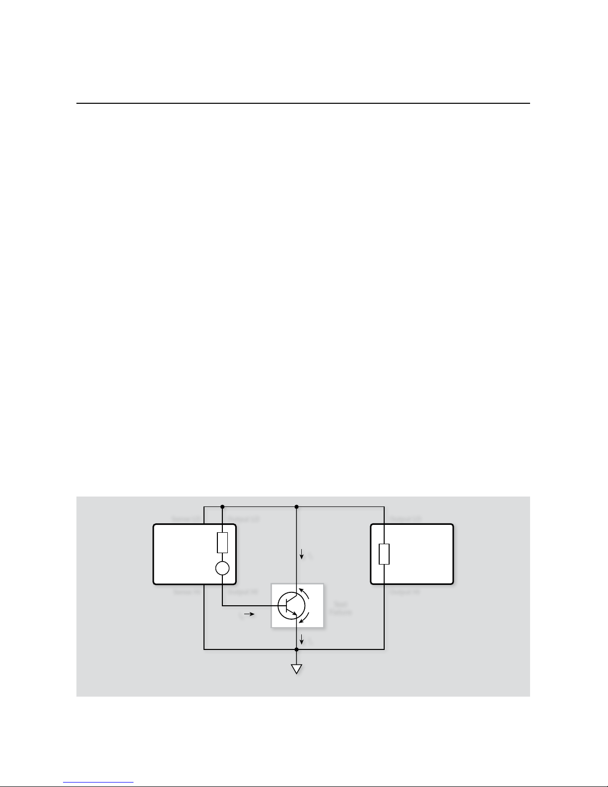
5.3.1 Program 12 Test Conﬁguration . . . . . . . 5-2

5.3.2 Example Program 12: Substrate Current

vs. Gate-Source Voltage . . . . . . . . . . . 5-2

5.3.3 Typical Program 12 Results . . . . . . . . . 5-4

5.3.4 Program 12 Description . . . . . . . . . . . 5-4

5.3.5 Modifying Program 12 . . . . . . . . . . . . 5-5

5.3.6 Program 13 Test Conﬁguration . . . . . . . 5-5

5.3.7 Example Program 13: Common-Source Characteristics with Source-Measure Unit

Substrate Bias . . . . . . . . . . . . . . . . 5-5

5.3.8 Typical Program 13 Results . . . . . . . . . 5-7

5.3.9 Program 13 Description . . . . . . . . . . . 5-7

5.3.10 Modifying Program 13 . . . . . . . . . . . . 5-7

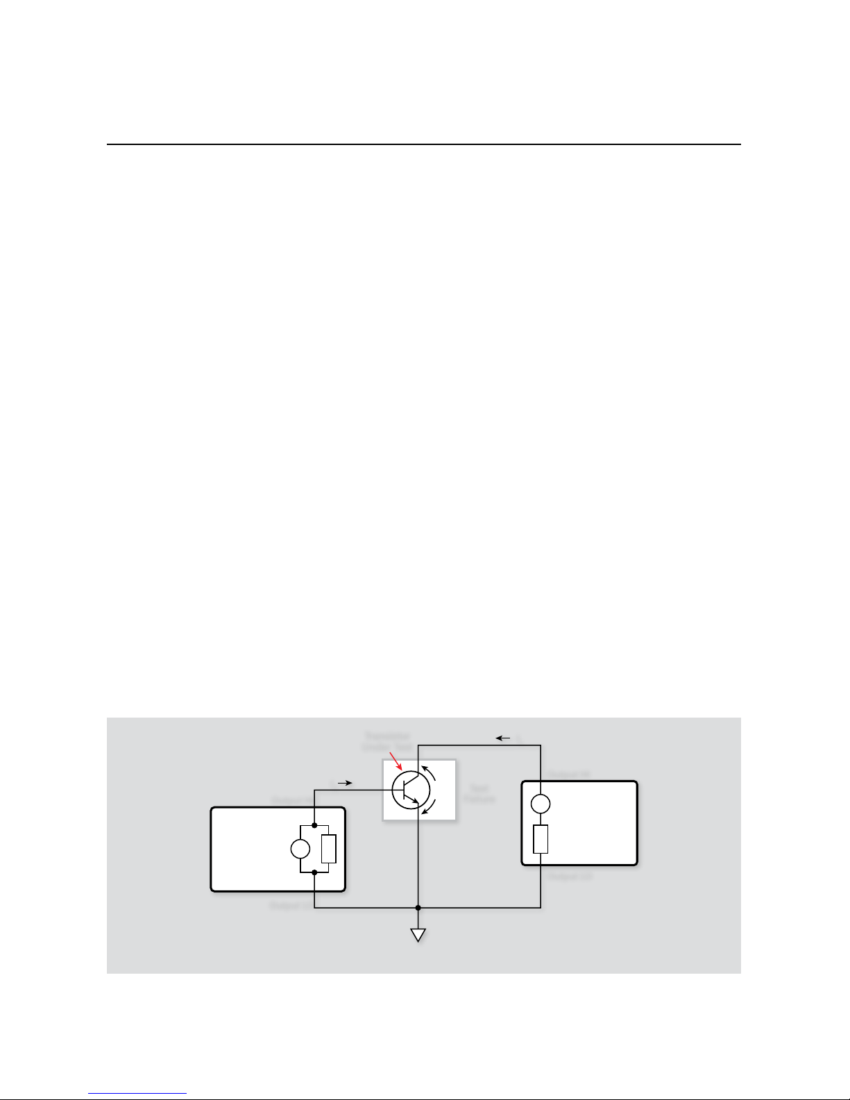
5.4 BJT Substrate Biasing. . . . . . . . . . . . . . . . 5-7

5.4.1 Program 14 Test Conﬁguration . . . . . . . 5-7

5.4.2 Example Program 14: Common-Emitter

Characteristics with a Substrate Bias . . . . 5-7

5.4.3 Typical Program 14 Results. . . . . . . . . . 5-9

5.4.4 Program 14 Description . . . . . . . . . . . 5-9

5.4.5 Modifying Program 14 . . . . . . . . . . . . 5-10

Section 6 High Power Tests

6.1 Introduction. . . . . . . . . . . . . . . . . . . . . 6-1

6.1.1 Program 15 Test Conﬁguration . . . . . . . 6-1

6.1.2 Example Program 15: High Current

Source and Voltage Measure . . . . . . . . . 6-1

6.1.3 Program 15 Description . . . . . . . . . . . 6-2

6.2 Instrument Connections . . . . . . . . . . . . . . 6-2

6.2.1 Program 16 Test Conﬁguration . . . . . . . 6-2

6.2.2 Example Program 16: High Voltage

Source and Current Measure . . . . . . . . 6-2

6.2.3 Program 16 Description . . . . . . . . . . . 6-3

Appendix A Scripts

Section 2. Two-Terminal Devices . . . . . . . . . . . . . A-1

Program 1. Voltage Coefﬁcient of Resistors . . . . . A-1

Program 2. Capacitor Leakage Test . . . . . . . . . A-5

Program 3. Diode Characterization . . . . . . . . . A-8

Program 3A. Diode Characterization Linear Sweep . A-8 Program 3B. Diode Characterization Log Sweep . . A -11 Program 3C. Diode Characterization Pulsed Sweep . A-14

Section 3. Bipolar Transistor Tests . . . . . . . . . . . . A-19

Program 4. Common-Emitter Characteristics . . . . A -19

Program 5. Gummel Plot . . . . . . . . . . . . . . . A-24

Section 6. High Power Tests. . . . . . . . . . . . . . . . A-28

Program 6. Current Gain . . . . . . . . . . . . . . . A-28

Program 6A. Current Gain (Search Method). . . . . A-28

Program 6B. Current Gain (Fast Method) . . . . . . A-32

Program 7. AC Current Gain . . . . . . . . . . . . . A-36

Program 8. Transistor Leakage (ICEO). . . . . . . . A-39

Section 4. FET Tests . . . . . . . . . . . . . . . . . . . . A-43

Program 9. Common-Source Characteristics . . . . A-43

Program 10. Transconductance . . . . . . . . . . . A-48

Program 11. Threshold . . . . . . . . . . . . . . . . A-52

Program 11A. Threshold (Search) . . . . . . . . . . A-52

Program 11B. Threshold (Fast). . . . . . . . . . . . A-56

Section 5. Using Substrate Bias . . . . . . . . . . . . . . A-60

Program 12. Substrate Current vs. Gate-Source

Voltage (FET ISB vs. VGS) . . . . . . . . . . . A-60

Program 13. Common-Source Characteristics

with Substrate Bias . . . . . . . . . . . . . A-64

Program 14. Common-Emitter Characteristics

with Substrate Bias . . . . . . . . . . . . . . A -71

Section 6. High Power Tests. . . . . . . . . . . . . . . . A-7 8

Program 15. High Current with

Voltage Measurement . . . . . . . . . . . . A-78

Program 16. High Voltage with

Current Measurement . . . . . . . . . . . . A-80

List of Illustrations

Section 1 General Information

Figure 1-1. Typical system conﬁguration for applications. . .1-1

Section 2 Two-terminal Device Tests

Figure 2-1. Series 2600 two-wire connections

(local sensing) . . . . . . . . . . . . . . . . . . . . . . .2-1

Figure 2-2. Voltage coefﬁcient test conﬁguration . . . . . . .2-1

Figure 2-3. Test conﬁguration for capacitor leakage test . . .2-3

Figure 2-4. Staircase sweep . . . . . . . . . . . . . . . . . .2-5

Figure 2-5. Test conﬁguration for diode characterization. . .2-5

Figure 2-6. Program 3 results: Diode forward

characteristics . . . . . . . . . . . . . . . . . . . . . . .2-6

Section 3 Bipolar Transistor Tests

Figure 3-1. Test conﬁguration for common-emitter tests . . 3-1

Figure 3-2. Program 4 results: Common-emitter

characteristics . . . . . . . . . . . . . . . . . . . . . . 3-3

Figure 3-3. Gummel plot test conﬁguration. . . . . . . . . 3-4

Figure 3-4. Program 5 results: Gummel plot . . . . . . . . 3-5

Figure 3-5. Test conﬁguration for current gain tests

using search method . . . . . . . . . . . . . . . . . . . 3-6

Figure 3-6. Test conﬁguration for fast current gain tests . . 3-8

Figure 3-7. Conﬁguration for I

CEO

tests . . . . . . . . . . . 3-11

Figure 3-8. Program 8 results: I

CEO

vs. V

CEO

. . . . . . . . . 3-12

Section 4 FET Tests

Figure 4-1. Test conﬁguration for common-source tests . . 4-2

Figure 4-2. Program 9 results: Common-source

characteristics . . . . . . . . . . . . . . . . . . . . . . 4-3

Figure 4-3. Conﬁguration for transductance tests . . . . . 4-4

Figure 4-4. Program 10 results: Transconductance vs. VGS . 4-5

Figure 4-5. Program 10 results: Transconductance vs. ID . . 4-5

Figure 4-6. Conﬁguration for search method

threshold tests . . . . . . . . . . . . . . . . . . . . . . 4-6

Figure 4-7. Conﬁguration for self-bias threshold tests . . . 4-8

Section 5 Using Substrate Bias

Figure 5-1. TSP-Link connections for two instruments . . . 5-1

Figure 5-2. TSP-Link instrument connections . . . . . . . . 5-2

Figure 5-3. Program 12 test conﬁguration . . . . . . . . . 5-3

Figure 5-4. Program 12 typical results: ISB vs. VGS . . . . . 5-4

Figure 5-5. Program 13 test conﬁguration. . . . . . . . . . 5-5

Figure 5-6. Program 13 typical results: Common-source

characteristics with substrate bias . . . . . . . . . . . . 5-6

Figure 5-7. Program 14 test conﬁguration . . . . . . . . . . 5-8

Figure 5-8. Program 14 typical results: Common-emitter

characteristics with substrate bias . . . . . . . . . . . . 5-9

Section 6 High Power Tests

Figure 6-1. High current (SMUs in parallel). . . . . . . . . 6-1

Figure 6-2. High voltage (SMUs in series) . . . . . . . . . . 6-2

Appendix A Scripts

1-1

Section 1

General Information

1.1 Introduction

The following paragraphs discuss the overall hardware and software conﬁgurations of the system necessary to run the example application programs in this guide.

1.2 Hardware Conﬁguration

1.2.1 System Conﬁguration

Figure 1-1 shows the overall hardware conﬁguration of a typical test system. The various components in the system perform a number of functions:

Series 2600 System SourceMeter Instruments: System Source Meter instruments are specialized test instruments capable of sourcing current and simultaneously measuring voltage, or sourcing current and simultaneously measuring voltage. A single Source-Measure Unit (SMU) channel is required when testing twoterminal devices such as resistors or capacitors. Three- and fourterminal devices, such as BJTs and FETs, may require two or more SMU channels. Dual-channel System SourceMeter instruments, such as the Models 2602, 2612, and 2636, provide two SMUs in a half-rack instrument. Their ease of programming, ﬂexible expansion, and wide coverage of source/measure signal levels make them ideal for testing a wide array of discrete components. Before starting, make sure the instrument you are using has the source and measurement ranges that will ﬁt your testing speciﬁcations.

Test ﬁxture: A test ﬁxture can be used for an external test circuit. The test ﬁxture can be a metal or nonmetallic enclosure, and is typically equipped with a lid. The test circuit is mounted inside the test ﬁxture. When hazardous voltages (>30Vrms, 42Vpeak) will be present, the test ﬁxture must have the following safety requirements:

WAR NING To provide protection from shock hazards, an enclosure should be provided that surrounds all live parts. Nonmetallic enclosures must be constructed of materials suitably rated for ﬂammability and the voltage and temperature requirements of the test circuit. For metallic enclosures, the test ﬁxture chassis must be properly connected to safety earth ground. A grounding wire (#18 AWG or larger) must be attached securely to the test ﬁxture at a screw terminal designed for safety grounding. The other end of the ground wire must be attached to a known safety earth ground.

Construction Material: A metal test ﬁxture must be connected to a known safety earth ground as described in the WARNING above.

WAR NING A nonmetallic test ﬁxture must be constructed of materials that are suitable for ﬂammability, voltage, and temperature conditions that may exist in the test circuit. The construction requirements for a nonmetallic enclosure are also described in the WARNING above.

Test Circuit Isolation: With the lid closed, the test ﬁxture must completely surround the test circuit. A metal test ﬁxture must be electrically isolated from the test circuit. Input/output connectors mounted on a metal test ﬁxture must also be isolated from the test ﬁxture. Internally, Teﬂon® standoffs are typically used to insulate the internal pc-board or guard plate for the test circuit from a metal test ﬁxture.

Interlock Switch: The test ﬁxture must have a normally open interlock switch. The interlock switch must be installed so that, when the lid of the test ﬁxture is opened, the switch will open, and when the lid is closed, the switch will close.

WAR NING

When an interlock is required for safety, a separate circuit should be provided that meets the requirements of the application to protect the operator reliably from exposed voltages. The output enable pin

Series 2600

System

SourceMeter

CPU

w/GPIB

GPIB

Cable

Output HI

Output LO

DUT

Figure 1-1. Typical system conﬁguration for applications

1-2

SECTION 1

General Information

on the digital I/O port on the Models 2601 and 2602 System SourceMeter instruments is not suitable for control of safety circuits and should not be used to control a safety interlock. The Interlock pin on the digital I/O port for the Models 2611, 2612, 2635, and 2636 can be used to control a safety interlock.

Computer: The test programs in this document require a PC with

IEEE-488 (GPIB) communications and cabling.

Software: Series 2600 System SourceMeter instruments each use a powerful on-board test sequencer known as the Test Script Processor (TSP™). The TSP is accessed through the instrument communications port, most often, the GPIB. The test program, or script, is simply a text ﬁle that contains commands that instruct the instrument to perform certain actions. Scripts can be written in many different styles as well as utilizing different programming environments. This guide discusses script creation and management using Keithley Test Script Builder (TSB), an easy-to-use program that allows you to create, edit, and manage test scripts. For more information on TSB and scripting, see Section 2: Using Test Script Builder of the Series 2600 Reference Manual.

Connections and Cabling: High quality cabling, such as the Keithley Model 2600-BAN or Model 7078-TRX-3 triaxial cables, should be used whenever possible.

1.2.2 Remote/Local Sensing Considerations

In order to simplify the test connections, most applications in this guide use local sensing for the SMUs. Local sensing requires

connecting only two cables between the SMUs and the test ﬁxture (OUTPUT HI and OUTPUT LO).

When sourcing and/or measuring voltage in a low impedance test circuit, there can be errors associated with IR drops in the test leads. Using four-wire remote sense connections optimizes voltage source and measure accuracy. When sourcing voltage, four-wire remote sensing ensures that the programmed voltage is delivered to the DUT. When measuring voltage, only the voltage drop across the DUT is measured. Use four-wire remote sensing for the following source-measure conditions:

Sourcing and/or measuring voltage in low impedance (<1k• W) test circuits.

Enforcing voltage compliance limit directly at the DUT.•

1.3 Graphing

All of the programs in this guide print the data to the TSB Instrument Console. In some cases, graphing the data can help you visualize the characteristics of the DUT. One method of graphing is to copy and paste the data from the TSB Instrument Console and place it in a spreadsheet program such as Microsoft Excel.

After the script has run, and the data has been returned to the Instrument Console, you can highlight it by using the PC’s mouse: depress the Control and c (commonly written as Ctrl+c) keys on the keyboard simultaneously, switch to an open Excel worksheet, and depress Control and v simultaneously (Ctrl+v). The data should now be placed in the open worksheet columns so you can use the normal graphing tools available in your spreadsheet program to graph the data as needed.

This Applications Guide is designed for Series 2600 instrument users who want to create their own scripts using the Test Script Builder software. Other options include LabTracer® 2 software, the Automated Characterization Suite (ACS), and a LabVIEW driver.

2-1

Section 2

Two-terminal Device Tests

2.1 Introduction

Two-terminal device tests discussed in this section include voltage coefﬁcient tests on resistors, leakage tests on capacitors, and diode characterization.

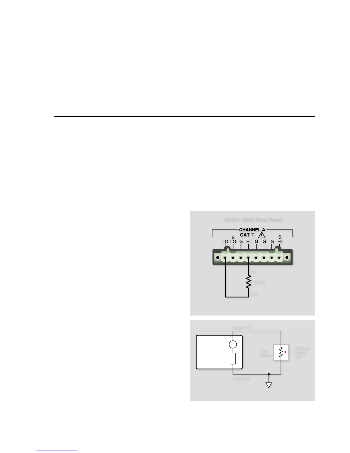
2.2 Instrument Connections

Figure 2-1 shows the instrument connections for two-terminal device tests. Note that only one channel of a Source-Measure Unit (SMU) is required for these applications. Be aware that multichannel models, such as the Model 2602, can be used, but are not required to run the test program.

WAR NING

Lethal voltages may be present. To avoid a possible shock hazard, the test system should be equipped with protective shielding and a safety interlock circuit. For more information on interlock techniques, see Section 10 of the Series 2600 Reference manual.

Turn off all power before connecting or disconnecting wires or cables.

NOTES

Remote sensing connections are recommended for optimum 1. accuracy. See paragraph 1.2.2 for details.

If measurement noise is a problem, or for critical, low level 2. applications, use shielded cable for all signal connections.

2.3 Voltage Coefﬁcient Tests of Resistors

Resistors often show a change in resistance with applied voltage with high megohm resistors (>109W) showing the most pronounced effects. This change in resistance can be characterized as the voltage coefﬁcient. The following paragraphs discuss voltage coefﬁcient tests using a single-channel Model 2601 System SourceMeter instrument. The testing can be performed using any of the Series 2600 System SourceMeter instruments.

2.3.1 Test Conﬁguration

The test conﬁguration for voltage coefﬁcient measurements is shown in Figure 2-2. One SMU sources the voltage across the resistor under test and measures the resulting current through the resistor.

2.3.2 Voltage Coefﬁcient Calculations

Two different current readings at two different voltage values are required to calculate the voltage coefﬁcient. Two resistance read-

DUT

Series 2600 Rear Panel

Figure 2-1. Series 2600 two-wire connections (local sensing)

Series 2600

System

SourceMeter

Channel A

Source V, Measure I

R = V/I

Test

Fixture

Resistor Under Test

Output HI

Output LO

Figure 2-2. Voltage coefﬁcient test conﬁguration

2-2

SECTION 2

Two-terminal Device Tests

ings, R1 and R2, are then obtained, and the voltage coefﬁcient in %/V can then be calculated as follows:

100 (R2 – R1) Voltage Coefﬁcient (%/V) =

__________

(V2 – V1)

where: R1 = resistance calculated with ﬁrst applied voltage (V1).

= resistance calculated with second applied voltage

(V2).

For example, assume that the following values are obtained:

= 1.01 × 1010W

= 1 × 1010W

(V2 – V1) = 10V

The voltage coefﬁcient is:

100 (1×103) Voltage Coefﬁcient (%/V) =

__________

= 0.1%/V

1×1 010 (10)

2.3.3 Measurement Considerations

A couple of points should be noted when using this procedure to determine the voltage coefﬁcient of high megohm resistors. Keep in mind that any leakage resistance in the test system will degrade the accuracy of your measurements. To avoid such problems, use only high quality test ﬁxtures that have insulation resistances greater than the resistances being measured. Using isolation resistances 10× greater than the measured resistance is a good rule of thumb. Also, make certain that the test ﬁxture sockets are kept clean and free of contamination as oils and dirt can lower the resistance of the ﬁxture and cause error in the measurement.

There is an upper limit on the resistance value that can be measured using this test conﬁguration. For one thing, even a well- designed test ﬁxture has a ﬁnite (although very high) path isolation value. Secondly, the maximum resistance is determined by the test voltage and current-measurement resolution of the test instrument. Finally, the instrument has a typical output impedance of 1015W. To maximize measurement accuracy with a given resistor, use the highest test voltages possible.

2.3.4 Example Program 1: Voltage Coefﬁcient Test

Program 1 demonstrates programming techniques for voltage coefﬁcient tests. Follow the steps that follow to use the test program. To reiterate, this test requires a single Source-Measure channel. For this example, we will refer to the single-channel Model 2601 System SourceMeter instrument. The test program

can be used with the multi-channel members of the Series 2600 family with no modiﬁcation.

With the power off, connect the Model 2601 System Source-1. Meter instrument to the computer’s IEEE-488 interface.

Connect the test ﬁxture to the instrument using appropriate 2. cables (see Figure 2-1).

Turn on the instrument, and allow the unit to warm up for 3. two hours for rated accuracy.

Turn on the computer and start Test Script Builder (TSB). Once 4. the program has started, open a session by connecting to the instrument. For details on how to use TSB, see the Series 2600 Reference Manual.

You can simply copy and paste the code from Appendix A 5. in this guide into the TSB script editing window (Program

1: Voltage Coefﬁcient), manually enter the code from the

appendix, or import the TSP ﬁle ‘Volt_Co.tsp’ after downloading it to your PC.

If your computer is currently connected to the Internet, you can click on this link to begin downloading: http://www.

keithley.com/data?asset=50914.

Install the resistor being tested in the test ﬁxture. The ﬁrst 6. step in the operation requires us ﬁrst to send the code to the instrument. The simplest method is to right-click in the open script window of TSB, and select ‘Run as TSP ﬁle’. This will compile the code and place it in the volatile run-time memory of the instrument. To store the program in non-volatile memory, see the “TSP Programming Fundamentals” section of the Series 2600 Reference Manual.

Once the code has been placed in the instrument run-time 7. memory, we can run it simply by calling the function ‘

Volt _

Co()

’. This can be done by typing the text ‘

Volt _ Co()

’ after

the active prompt in the Instrument Console line of TSB.

In the program 8. ‘Volt_ Co.tsp’, the function

Volt _

Co(v1src, v2src)

is created. The variables

v1src

and

v2src

represent the two test voltage values applied to the device-under-test (DUT). If they are left blank, the function will use the default values given to these variables, but you can specify what voltages are applied by simply sending voltages that are in-range in the function call. As an example, if you wanted to source 2V followed by 10V, simply send

Volt _

Co(2, 10)

to the instrument.

The instrument will then source the programmed voltages 9. and measure the respective currents through the resistor. The calculated voltage coefﬁcient and two resistance values will then be displayed in the Instrument Console window of TSB.

2-3

SECTION 2

Two-terminal Device Tests

2.3.5 Typical Program 1 Results

The actual voltage coefﬁcient you obtain using the program will, of course, depend on the resistor being tested. The typical voltage coefﬁcient obtained for a 10GW resistor (Keithley part number R-319-10G) was about 8ppm/V (0.008%/V).

2.3.6 Program 1 Description

At the start of the program, the instrument is reset to default conditions, and the error queue and data storage buffers are cleared. The following conﬁguration is then applied before the data collection begins:

Source V, DC mode•

Local sense•

100mA compliance, autorange measure•

1NPLC line cycle integration•

v1src:

• 100V

v2src:

• 200V

The instrument then sources

v1src

, checks the source for com-

pliance in the function named

Check _ Comp()

, and performs a measurement of the current if compliance is false. The source then applies

v2src

and performs a second current measurement.

The function

Calc _ Val()

then performs the calculation of the voltage coefﬁcient based on the programmed source values and the measured current values as described in Section 2.3.2, Voltage

Coefﬁcient Calculations.

The instrument output is then turned off and the function

Pri nt _ Data()

is run to print the data to the TSB window.

Note: If the compliance is true, the instrument will abort the program and print a warning to the TSB window. Check the DUT and cabling to make sure everything is connected correctly and re-run the test.

2.4 Capacitor Leakage Test

One important parameter associated with capacitors is leakage current. Once the leakage current is known, the insulation resistance can be easily calculated. The amount of leakage current in a capacitor depends both on the type of dielectric as well as the applied voltage. With a test voltage of 100V, for example, ceramic dielectric capacitors have typical leakage currents in the nanoamp to picoamp range, while polystyrene and polyester dielectric capacitors exhibit a much lower leakage current—typically in the femtoamp (10

–15

A) range

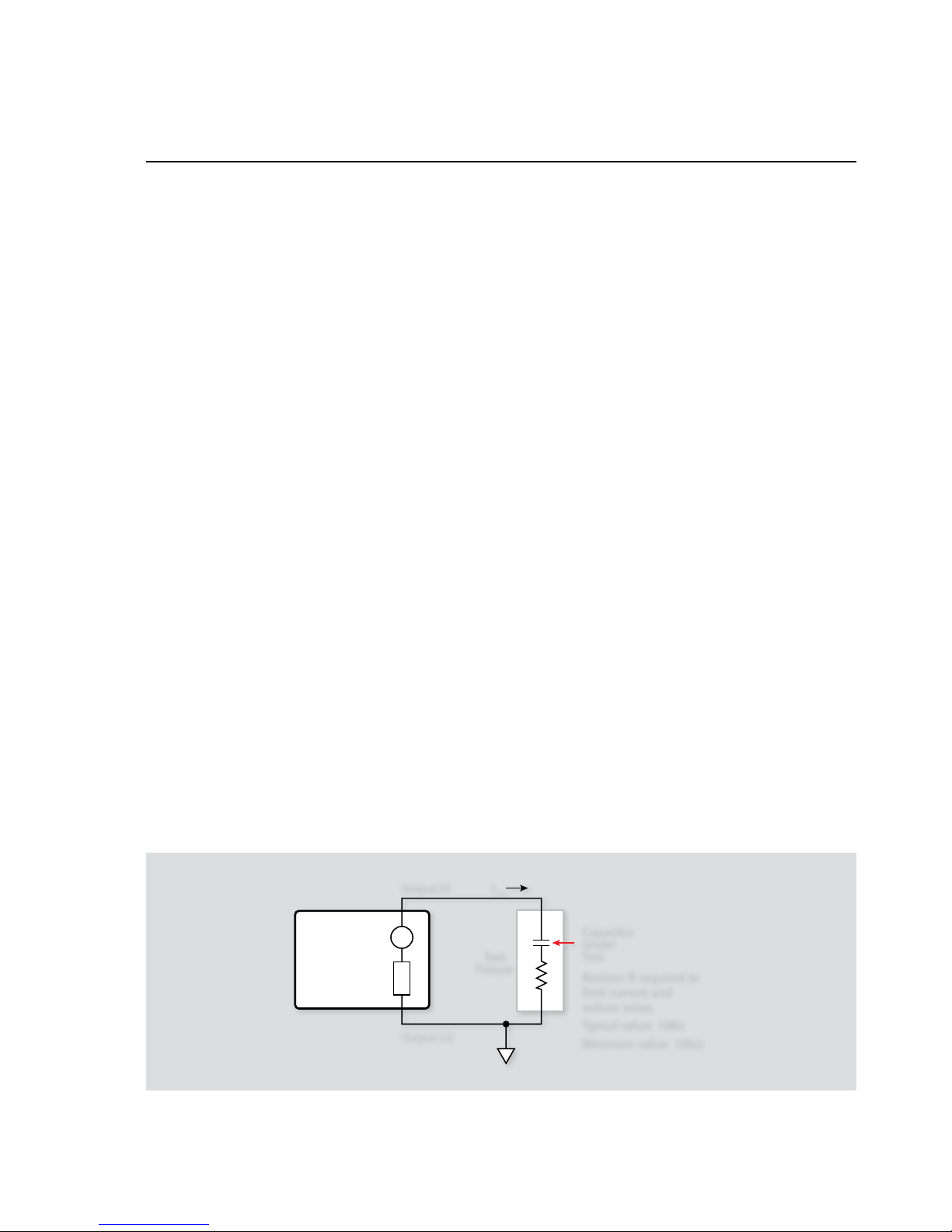
2.4.1 Test Conﬁguration

Figure 2-3 shows the test conﬁguration for the capacitor leakage test. The instrument sources the test voltage across the capacitor, and it measures the resulting leakage current through the device. The resistor, R, is included for current limiting, and it also helps to reduce noise. A typical value for R is 1MW, although that value can be decreased for larger capacitor values. Note, however, that values less than 10kW are not recommended.

2.4.2 Leakage Resistance Calculations

Once the leakage current is known, the leakage resistance can easily be calculated from the applied voltage and leakage current value as follows:

R = V/I

Resistor R required to limit current and reduce noise.

Typical value: 1MΩ Minimum value: 10kΩ

Series 2600

System

SourceMeter

Channel A

Source V,

Measure I

Test

Fixture

Capacitor Under Test

Output HI I

LKG

Output LO

Figure 2-3. Test conﬁguration for capacitor leakage test

2-4

SECTION 2

Two-terminal Device Tests

For example, assume that you measured a leakage current of 25nA with a test voltage of 100V. The leakage resistance is simply:

R =100/25nA = 4GW (4 × 109W)

2.4.3 Measurement Considerations

After the voltage is applied to the capacitor, the device must be allowed to charge fully before the current measurement can be made. Otherwise, an erroneous current, with a much higher value, will be measured. The time period during which the capacitor charges is often termed the “soak” time. A typical soak time is seven time constants, or 7RC, which would allow settling to less than 0.1% of ﬁnal value. For example, if R is 1MW, and C is 1µF, the recommended soak time is seven seconds. With small leakage currents (<1nA), it may be necessary to use a ﬁxed measurement range instead of auto ranging.

2.4.4 Example Program 2: Capacitor Leakage Test

Program 2 performs the capacitor leakage test described above. Follow the steps that follow to run the test using this program.

WAR NING

Hazardous voltage may be present on the capacitor leads after running this test. Discharge the capacitor before removing it from the test ﬁxture.

With the power off, connect the instrument to the computer’s 1. IEEE-488 interface.

Connect the test ﬁxture to the instrument using appropriate 2. cables.

Turn on the instrument, and allow the unit to warm up for 3. two hours for rated accuracy.

You can simply copy and paste the code from Appendix A in 5. this guide into the TSB script editing window (Program 2), manually enter the code from the appendix, or import the TSP ﬁle ‘Cap_Leak.tsp’ after downloading it to your PC.

If your computer is currently connected to the Internet, you can click on this link to begin downloading: http://www.

keithley.com/data?asset=50927.

Discharge and install the capacitor being tested, along with 6. the series resistor, in the appropriate axial component sockets of the test ﬁxture.

WAR NING Care should be taken when discharging the capacitor, as the voltage present may represent a shock hazard!

Now, we must send the code to the instrument. The simplest 7. method is to right-click in the open script window of TSB, and select ‘Run as TSP ﬁle’. This will compile the code and place it in the volatile run-time memory of the instrument. To store the program in non-volatile memory, see the “TSP Programming Fundamentals” section of the Series 2600 Reference Manual.

Once the code has been placed in the instrument run-time 8. memory, we can run it at any time simply by calling the function ‘

Cap _ Le a k()

’. This can be done by typing the text

‘

Cap _ Le a k()

’ after the active prompt in the Instrument

Console line of TSB.

In the program ‘9. Cap_Leak.tsp’, the function

Cap _

Lea k(v sr c)

is created. The variable

vsrc

represents the test voltage value applied to the device-under-test (DUT). If it is left blank, the function will use the default value given to the variable, but you can specify what voltage is applied by simply sending a voltage that is in-range in the function call. As an example, if you wanted to source 100V, simply send

Cap _ Le a k(100)

to the instrument.

The instrument will then source the programmed voltage and 10. measure the respective current through the capacitor. The measured current leakage and calculated resistance value will then be displayed in the Instrument Console window of TSB.

NOTE

The capacitor should be fully discharged before running the test. This can be accomplished by sourcing 0V on the device for the soak time or by shorting the leads together. Care should be taken because some capacitors can hold a charge for a signiﬁcant period of time and could pose an electrocution risk.

The soak time, denoted in the code as the variable

l _ soak

, has a default value of 10s. When entering the soak time, choose a value of at least 7RC to allow settling to within 0.1% of ﬁnal value. At very low currents (<500fA), a longer settling time may be required to compensate for dielectric absorption, especially at high voltages.

2.4.5 Typical Program 2 Results

As pointed out earlier, the exact value of leakage current will depend on the capacitor value as well as the dielectric. A typical value obtained for 1µF aluminum electrolytic capacitor was about 80nA at 25V.

2-5

SECTION 2

Two-terminal Device Tests

2.4.6 Program 2 Description

At the start of the program, the instrument is reset to default conditions, the error queue, and data storage buffers are cleared. The following conﬁguration is then applied before the data collection begins:

Source V, DC mode•

Local sense•

10mA compliance, autorange measure•

1 NPLC Line cycle integration•

vsrc:

• 40V

The instrument then sources

vsrc

, checks the source for compli-

ance in the function named

Check _ Comp()

, and performs a

measurement of the current if compliance is false.

The function

Calc _ Val()

then performs the calculation of the leakage resistance based on the programmed source value and the measured current value as described in paragraph 2.4.2,

Leakage Resistance Calculations.

The instrument output is then turned off and the function

Pri nt _ Data()

is run to print the data to the TSB window.

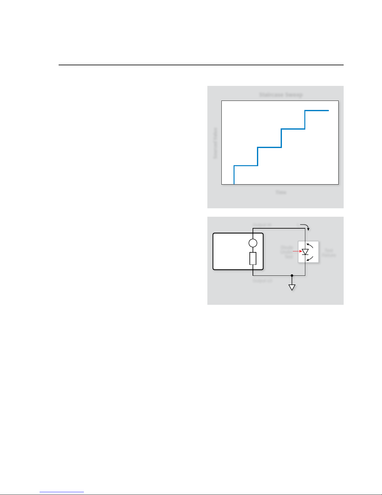
2.5 Diode Characterization

The System SourceMeter instrument is ideal for characterizing diodes because it can source a current through the device, and measure the resulting forward voltage drop (VF) across the device. A standard technique for diode characterization is to perform a staircase sweep (Figure 2-4) of the source current from a starting value to an end value while measuring the voltage at each current step. The following paragraphs discuss the test conﬁguration and give a sample test program for such tests.

2.5.1 Test Conﬁguration

Figure 2-5 shows the test conﬁguration for the diode characterization test. The System SourceMeter instrument is used to source the forward current (IF) through the diode under test, and it also measures the forward voltage (VF) across the device. IF is swept across the desired range of values, and VF is measured at each current. Note that the same general conﬁguration could be used to

measure leakage current by reversing the diode, sourcing voltage, and measuring the leakage current.

2.5.2 Measurement Considerations

Because the voltages being measured will be fairly small (≈0.6V), remote sensing can be used to minimize the effects of voltage drops across the test connections and in the test ﬁxture. Remote sensing requires the use of the Sense connections on the System SourceMeter channel being used, as well as changing the code to reﬂect remote sensing. For more information on remote sensing, see the Series 2600 Reference Manual.

2.5.3 Example Program 3: Diode Characterization

Program 3 demonstrates the basic programming techniques for running the diode characterization test. Follow these steps to use this program:

Staircase Sweep

Time

Sourced Value

Figure 2-4. Staircase sweep

Test

Fixture

Diode

Under

Test

Output HI

Output LO

Series 2600

System

SourceMeter

Channel A

Sweep I

Measure V

Figure 2-5. Test conﬁguration for diode characterization

2-6

SECTION 2

Two-terminal Device Tests

With the power off, connect the instrument to the computer’s 1. IEEE-488 interface.

Connect the test ﬁxture to the instrument using appropriate 2. cables.

Turn on the instrument, and allow the unit to warm up for 3. two hours for rated accuracy.

You can simply copy and paste the code from Appendix A in 5. this guide into the TSB script editing window (Program 3A,

Diode Forward Characterization), manually enter the code

from the appendix, or import the TSP ﬁle ‘Diode_Fwd_Char. tsp’ after downloading it to your PC.

If your computer is currently connected to the Internet, you can click on this link to begin downloading: http://www.

keithley.com/data?asset=50924.

Install a small-signal silicon diode such as a 1N914 or 1N4148 6. in the appropriate axial socket of the test ﬁxture.

Now, we must send the code to the instrument. One method 7. is simply to right-click in the open script window of TSB, and select ‘Run as TSP ﬁle’. This will compile the code and place it in the volatile run-time memory of the instrument. To store the program in non-volatile memory, see the “TSP Programming Fundamentals” section of the Series 2600 Reference Manual.

Once the code has been placed in the instrument run-time 8. memory, we can run it at any time simply by calling the function ‘Diode_Fwd_Char()’. This can be done by typing the text ‘

Dio de _ F w d _ Ch ar()

’ after the active prompt in the

Instrument Console line of TSB.

In the program ‘Diode_Fwd_Char.tsp’, the function 9.

Diode _

Fwd _ Char(ilevel, start, stop, steps)

created. The variable

ilevel

represents the current value applied to the device-under-test (DUT) both before and after the staircase sweep has been applied. The

start

variable represents the starting current value for the sweep, stop represents the end current value, and steps represents the number of steps in the sweep. If any values are left blank, the function will use the default value given to that variable, but you can specify what voltage is applied by simply sending a voltage that is in-range in the function call.

As an example, if you wanted to conﬁgure a test that would 10. source 0mA before and after the sweep, with a sweep start value of 1mA, stop value of 10mA, and 10 steps, you would

simply send

Diode _ Fwd _ Char(0, 0.001, 0.01,

10)

to the instrument.

The instrument will then source the programmed current 11. staircase sweep and measure the respective voltage at each step. The measured and sourced values are then printed to the screen (if using TSB). To graph the results, simply copy and paste the data into a spreadsheet such as Microsoft Excel and chart.

2.5.4 Typical Program 3 Results

Figure 2-6 shows typical results obtained using Example Program

3. These results are for a 1N914 silicon diode.

2.5.5 Program 3 Description

Source I•

Local sense•

10V compliance, autorange measure•

Ile v el:

• 0A

star t:

• 0.001 A

stop:

• 0.01A

steps:

• 10

The instrument then sources

ilevel

, dwells

l _ delay

sec-

onds, and begins the staircase sweep from

start

stop

in steps. At each current step, both the current and voltage are measured.

Diode Forward Characteristics

Current (Amps)

Voltage Data (V)

Voltage (Volts)

9.00E–01

8.00E–01

7.00E–01

6.00E–01

5.00E–01

4.00E–01

3.00E–01

2.00E–01

1.00E–01

0.00E–00

0.00E+00 2.00E–03 4.00E–03 6.00E–03 8.00E–03 1. 00E–02

Figure 2-6. Program 3 results: Diode forward characteristics

2-7

SECTION 2

Two-terminal Device Tests

The instrument output is then turned off and the function

Pri nt _ Data()

is run to print the data to the TSB window. To graph the results, simply copy and paste the data into a spreadsheet such as Microsoft Excel and chart.

2.5.6 Using Log Sweeps

With some devices, it may be desirable to use a log sweep because of the wide range of currents necessary to perform the test. Pro-

gram 3B performs a log sweep of the diode current.

If your computer is currently connected to the Internet, you can click on this link to begin downloading ‘Diode_Fwd_Char_Log. tsp’: http://www.keithley.com/data?asset=50923.

Note that the start and stop currents are programmed just as before, although with a much wider range than would be practical with a linear sweep. With log sweep, however, the

points

pa rameter, which deﬁnes the number of points per decade, replaces the steps parameter that is used with the linear sweep.

To run the Log sweep, we must send the code to the instrument. One method is simply to right-click in the open script window of TSB, and select ‘Run as TSP ﬁle’. This will compile the code

and place it in the volatile run-time memory of the instrument. To store the program in non-volatile memory, see the “TSP Programming Fundamentals” section of the Series 2600 Reference Manual.

Once the code has been placed in the instrument run-time memory, we can run it at any time simply by calling the function ‘Diode_Fwd_Char_Log()’. This can be done by typing the text ‘

Diode _ Fwd _ Char _ Log()

’ after the active prompt in the

Instrument Console line of TSB.

2.5.7 Using Pulsed Sweeps

In some cases, it may be desirable to use a pulsed sweep to avoid device self-heating that could affect the test results. Program 3C performs a staircase pulse sweep. In this program, there are two additional variables ton and toff, where ton is the source on duration and toff is the source off time for the pulse. During the toff portions of the sweep, the source value is returned to the ilevel bias value.

If your computer is currently connected to the Internet, you can click on this link to begin downloading ‘Diode_Fwd_Char_Pulse. tsp’: http://www.keithley.com/data?asset=50922.

2-8

SECTION 2

Two-terminal Device Tests

3-1

Section 3

Bipolar Transistor Tests

3.1 Introduction

Bipolar transistor tests discussed in this section include: tests to generate common-emitter characteristic curves, Gummel plot, current gain, and transistor leakage tests.

3.2 Instrument Connections

Figure 3-1 shows the instrument connections for the bipolar transistor tests outlined in this section. Two Source-Measure channels are required for the tests (except for the leakage current test, which requires only one Source-Measure channel).

Keithley Model 2600-BAN cables or Model 7078-TRX-3 low noise triaxial cables are recommended to make instrument-to-test ﬁxture connections. In addition, the safety interlock connecting cables must be connected to the instrument and ﬁxture if using instrumentation capable of producing greater than 42V.

WAR NING

Lethal voltages may be exposed when working with test ﬁxtures. To avoid a possible shock hazard, the ﬁxture must be equipped with a working safety interlock circuit. For more information on the

interlock of the Series 2600, please see the Series 2600 Reference Manual.

NOTES

Remote sensing connections are recommended for optimum accuracy. See paragraph 1.2.2 for details.

If measurement noise is a problem, or for critical, low level applications, use shielded cable for all signal connections.

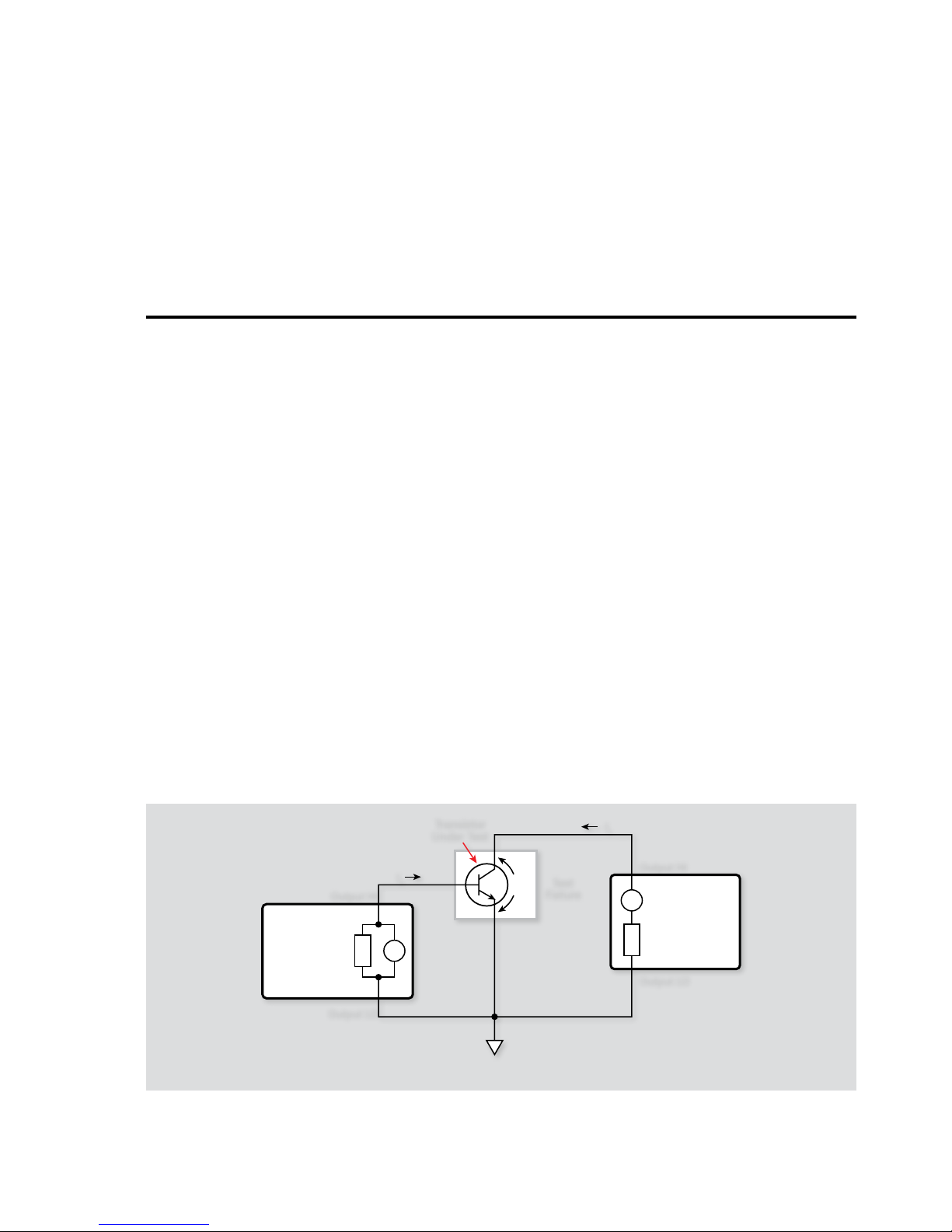
3.3 Common-Emitter Characteristics

Common-emitter characteristics are probably the most familiar type of curves generated for bipolar transistors. Test data used to generate these curves is obtained by sweeping the base current (IB) across the desired range of values at speciﬁc increments. At each be current value, the collector-emitter voltage (VCE) is swept across the desired range, again at speciﬁc increments. At each VCE value, the collector current (IC) is measured.

Once the data is collected, it is conveniently printed (if using TSB). You can then use the copy-and-paste method to place the data into a spreadsheet program such as Microsoft Excel. Common

Series 2600

System

SourceMeter

Channel A

Sweep V

Measure I

Series 2600

System

SourceMeter

Channel B

Sweep I

Test

Fixture

Transistor

Under Test

Output HI

Output LO

Figure 3-1. Test conﬁguration for common-emitter tests

3-2

SECTION 3

Bipolar Transistor Tests

plotting styles include graphing IC vs. VCE for each value of IB. The result is a family of curves that shows how IC varies with VCE at speciﬁc IB values.

3.3.1 Test Conﬁguration

Figure 3-1 shows the test conﬁguration for the common-emitter characteristic tests. Many of the transistor tests performed require two Source-Measure Units (SMUs). The Series 2600 System SourceMeter instruments have dual-channel members such as the Model 2602, 2612, and 2636. This offers a convenient transistor test system all in one box. The tests can be run using two singlechannel instruments, but the code will have to be modiﬁed to do so.

In this test, SMUB sweeps IB across the desired range, and SMUA sweeps VCE and measures IC. Note that an NPN transistor is shown as part of the test conﬁguration. A small-signal NPN transistor with an approximate current gain of 500 (such as a 2N5089) is recommended for use with the test program below. Other similar transistors such as a 2N3904 may also be used, but the program may require modiﬁcation.

3.3.2 Measurement Considerations

A ﬁxed delay period of 100ms, which is included in the program, may not be sufﬁcient for testing some devices. Also, it maybe necessary to change the programmed current values to optimize the tests for a particular device.

3.3.3 Example Program 4: Common-Emitter Characteristics

Program 4 can be used to run common-emitter characteristic tests on small-signal NPN transistors. In order to run the program, follow these steps:

With the power off, connect a dual-channel System Source-1. Meter instrument to the computer’s IEEE-488 interface.

Connect the test ﬁxture to both units using appropriate cables 2. (see Figure 3-1).

Turn on the instrument and allow the unit to warm up for two 3. hours for rated accuracy.

You can simply copy and paste the code from Appendix A in 5. this guide into the TSB script editing window (Program 4), manually enter the code from the appendix, or import the TSP ﬁle ‘BJT_Comm_Emit.tsp’ after downloading it to your PC.

If your computer is currently connected to the Internet, you can click on this link to begin downloading: http://www.

keithley.com/data?asset=50930.

Install an NPN transistor such as a 2N5089 in the appropriate 6. transistor socket of the test ﬁxture.

Once the code has been placed in the instrument run-time 8. memory, we can run it at any time simply by calling the function ‘

BJT _ Comm _ Emit()

’. This can be done by typing

the text ‘

BJT _ Comm _ Emit()

’ after the active prompt in

the Instrument Console line of TSB.

In the program ‘9. BJT_Comm_Emit.tsp’, the function

BJT _ Comm _ Emit(istart, istop, isteps, vstart, vstop, vsteps)

is created.

istart

• represents the sweep start current value on the base of the transistor

istop

• represents the sweep stop value

isteps

• is the number of steps in the base current sweep

vstart

• represents the sweep start voltage value on the collector-emitter of the transistor

vstop

• represents the sweep stop voltage value

vsteps

• is the number of steps in the base current sweep

If these values are left blank, the function will use the default values given to the variables, but you can specify each variable value by simply sending a number that is in-range in the function call. As an example, if you wanted to have the base current swept from 1µA to 100µA in 10 steps, and the collector-emitter voltage (V

CEO

) to be swept from 0 to 10V in 1V steps, you would

send

BJT _ Comm _ Emit(1E-6, 100E-6, 10, 0, 10,

10)

to the instrument.

The instrument will then source the programmed start current 10. on the base, sweep the voltage on the collector-emitter, and measure the respective current through the collector-emitter. The base current will be incremented and the collector-emitter sweep will take place again. After the ﬁnal base source value and associated collector-emitter sweep, the collector-emitter voltage (VCE), measured collector-emitter current (ICE), and base current (IB) values will then be displayed in the Instrument Console window of TSB.

3-3

SECTION 3

Bipolar Transistor Tests

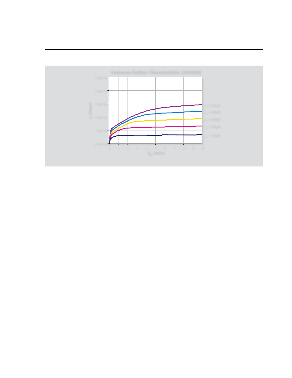
3.3.4 Typical Program 4 Results

Figure 3-2 shows typical results generated by Example Program 4. A 2N5089 NPN transistor was used to generate these test results.

3.3.5 Program 4 Description

For the following program description, refer to the program listing below.

Source I•

IV compliance, 1.1V range•

Local sense•

istart

• current: 10M

istop

• current: 50µA

isteps

• : 5

Following SMUB setup, SMUA, which sweeps VCE and measures IC, is programmed as follows:

Source V•

Local sensing•

100mA compliance, autorange measure•

1 NPLC Line cycle integration (to reduce noise)•

vstart

• : 0V

vstop

• : 10V

vsteps

• : 100

Once the two units are conﬁgured, the SMUB sources

istart

SMUA sources

vstart

, and the voltage (VCE) and current (ICE)

for SMUA are measured. The source value for SMUA is then incremented by

l _ vstep

, and the sweep is continued until

the source value reaches

vstop

. Then, SMUB is incremented by

l_istep

and SMUA begins another sweep from

vstart

vstop

vsteps

. This nested sweeping process continues until

SMUB reaches

istop

The instrument output is then turned off and the function

Pri nt _ Data()

is run to print the data to the TSB window. To graph the results, simply copy and paste the data into a spreadsheet such as Microsoft Excel and chart.

3.4 Gummel Plot

A Gummel plot is often used to determine current gain variations of a transistor. Data for a Gummel plot is obtained by sweeping the base-emitter voltage (VBE) across the desired range of values at speciﬁc increments. At each VBE value, both the base current (IB) and collector current (IC) are measured.

Once the data are taken, the data for IB, IC, and VBE is returned to the screen. If using TSB, a plot can be generated using the “copyand-paste” method in a spreadsheet program such as Microsoft Excel. Because of the large differences in magnitude between IB and IC, the Y axis is usually plotted logarithmically.

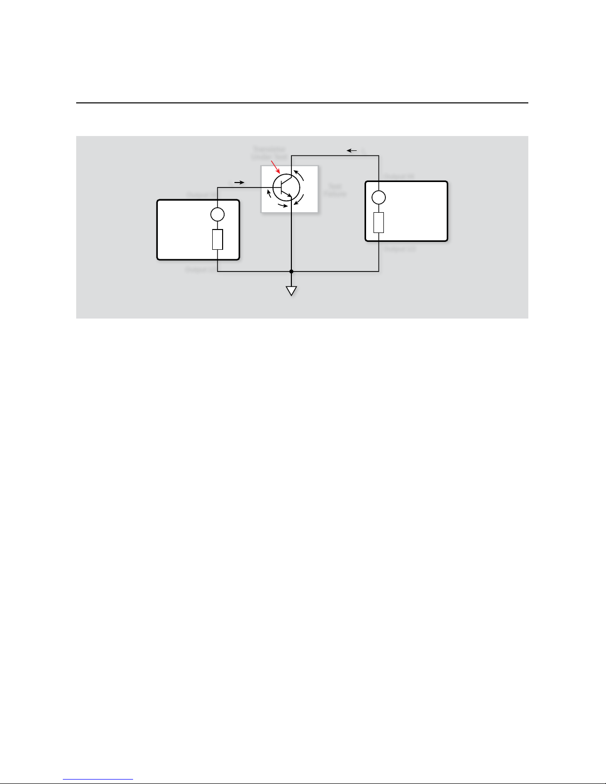
3.4.1 Test Conﬁguration

Figure 3-3 shows the test conﬁguration for Gummel plot tests. SMUB is used to sweep VBE across the desired range, and it also

Common-Emitter Characteristics (2N5089)

VBE (Volts)

IB = 10µA

= 20µA

= 30µA

= 40µA

IB = 50µA

(Amps)

5.00E–02

4.00E–02

3.00E–02

2.00E–02

1.00E–02

0.00E+00 0 1 2 3 4 5 6 7 8 9 10

Figure 3-2. Program 4 results: Common-emitter characteristics

3-4

SECTION 3

Bipolar Transistor Tests

measures IB. SMUA sets VCE to the desired ﬁxed value, and it also measures IC.

Due to the low current measurements associated with this type of testing, the Keithley Model 2636 System SourceMeter instrument is recommended. Its low level current measurement capabilities and dual-channel conﬁguration are ideal for producing high quality Gummel plots of transistors.

3.4.2 Measurement Considerations

As written, the range of VBE test values is from 0V to 0.7V in 0.01V increments. It may be necessary, however, to change these limits for best results with your particular device. Low currents will be measured so take the usual low current precautions.

3.4.3 Example Program 5: Gummel Plot

Program 5 demonstrates the basic programming techniques for generating a Gummel plot. Follow these steps to run this program:

With the power off, connect a dual-channel System Source-1. Meter instrument to the computer’s IEEE-488 interface.

Connect the test ﬁxture to both units using appropriate 2. c a b l e s .

Turn on the instrument and allow the unit to warm up for two 3. hours for rated accuracy.

You can simply copy and paste the code from Appendix A in 5. this guide into the TSB script editing window (Program 5), manually enter the code from the appendix, or import the TSP ﬁle ‘Gummel.tsp’ after downloading it to your PC.

If your computer is currently connected to the Internet, you can click on this link to begin downloading: http://www.

keithley.com/data?asset=50918

Install an NPN transistor such as a 2N5089 in the appropriate 6. transistor socket of the test ﬁxture.

Once the code has been placed in the instrument run-time 8. memory, we can run it at any time simply by calling the function ‘Gummel()’. This can be done by typing the text ‘

G u m m e l()

’ after the active prompt in the Instrument Con-

sole line of TSB.

In the program ‘Gummel.tsp’, the function 9.

Gummel

(vbestart, vbestop, vbesteps, vcebias)

created.

vbestart

• represents the sweep start voltage value on the base of the transistor

vbestop

• represents the sweep stop value

vbesteps

• is the number of steps in the base voltage sweep

Series 2600

System

SourceMeter

Channel A

Source V

Measure I

Series 2600

System

SourceMeter

Channel B

Sweep V

Measure I

Test

Fixture

Transistor

Under Test

Output HI

Output LO

Figure 3-3. Gummel plot test conﬁguration

3-5

SECTION 3

Bipolar Transistor Tests

vcebias

• represents the voltage bias value on the collector-emitter of the transistor

If these values are left blank, the function will use the default values given to the variables, but you can specify each variable value by simply sending a number that is in-range in the function call. As an example, if you wanted to have the base voltage swept from 0.1V to 1V in 10 steps, and the collector-emitter voltage (VCE) to be biased 5V, you would send

G u m m e l(0.1,

1, 10, 5)

to the instrument.

The base-emitter voltage will be swept between 0V and 0.7V in 10.

0.01V increments, and both IB and IC will be measured at each VBE value. Note that a ﬁxed collector-emitter voltage of 10V is used for the tests.

Once the sweep has been completed, the data (I11.

, IC, and VBE)

will be presented in the Instrument Console window of TSB.

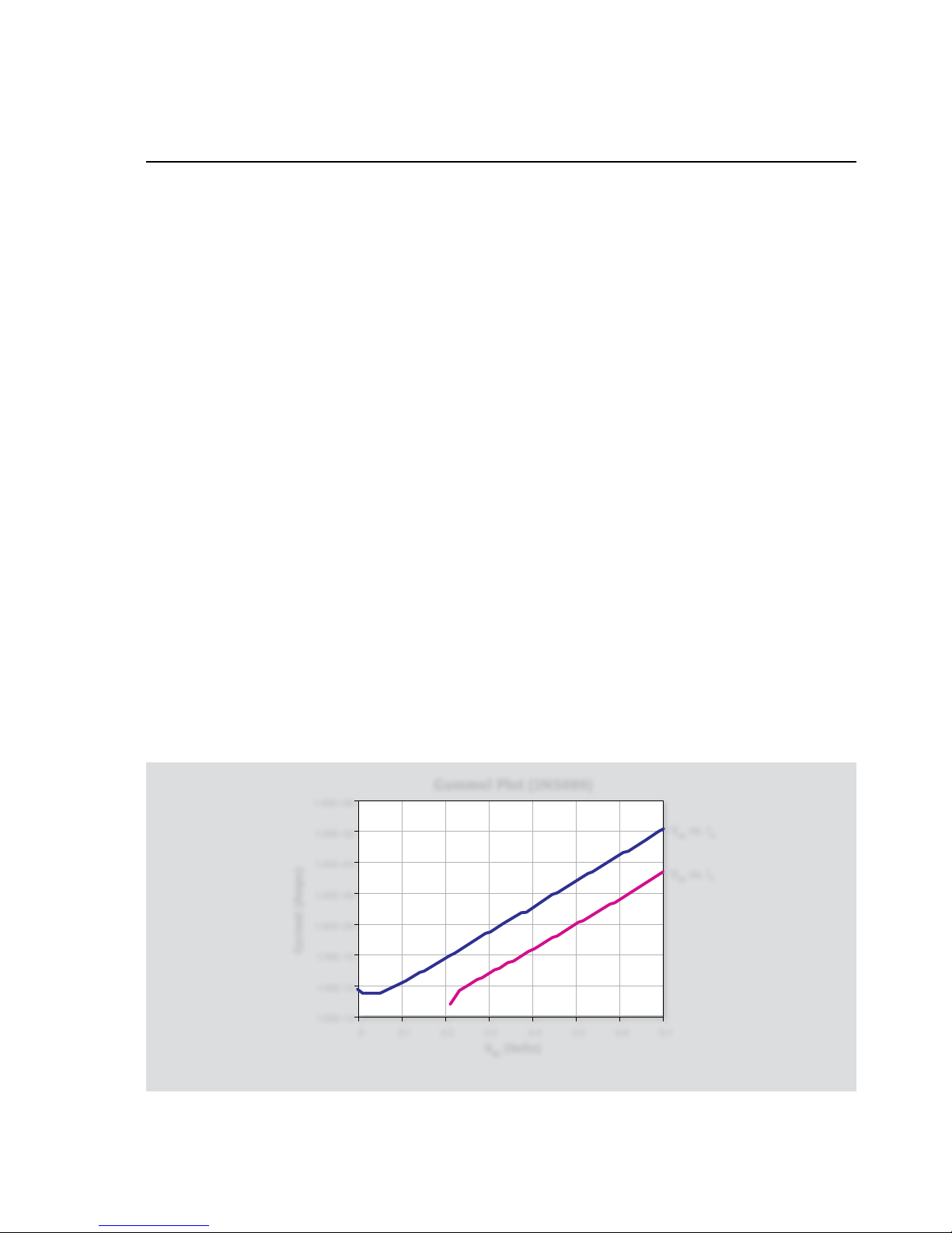
3.4.4 Typical Program 5 Results

Figure 3-4 displays a typical Gummel plot as generated by Example Program 5. Again, the transistor used for this example was a 2N5089 NPN silicon transistor.

3.4.5 Program 5 Description

SMUB, which sweeps VBE and measures IB, is set up as follows:

Source V•

1mA compliance, autorange measure•

Local sensing•

1 NPLC Line cycle integration•

vbestart

• : 0V

vbestop

• : 0.7V

vbesteps

• : 70

SMUA, which sources VCE and measures IC, is programmed in the following manner:

Source V•

Local sensing•

100mA compliance, autorange measure•

1 NPLC Line cycle integration•

Constant sweep (number of points programmed to 71), • VCE = 10V

vcebias

• : 10V

Following unit setup, both unit triggers are armed, and the instruments are placed into the operate mode (lines 320 and 330).

Once triggered, SMUB sets VBE to the required value, and SMUA then sets VCE and measures IC at IB. At the end of its measurement, SMUB increments VBE and the cycle repeats until VBE reaches the value set for

vbestop

During the test, VBE, IB, and IC are measured. Once the test has completed, the data is written to the Instrument Console of TSB and can be graphed in a spreadsheet program using the “copyand-paste” method of data transfer.

Gummel Plot (2N5089)

VBE (Volts)

vs. I

VBE vs. I

Current (Amps)

1.00E+00

1.00E–02

1.00E–04

1.00E–06

1.00E–08

1.00E–10

1.00E–12

1.00E–14

0 0.1 0.2 0.3 0.4 0.5 0.6 0.7

Figure 3-4. Program 5 results: Gummel plot

3-6

SECTION 3

Bipolar Transistor Tests

3.5 Current Gain

The following paragraphs discuss two methods for determining DC current gain, as well as ways to measure AC current gain.

3.5.1 Gain Calculations

The common-emitter DC current gain of a bipolar transistor is simply the ratio of the DC collector current to the DC base current of the device. The DC current gain is calculated as follows:

IC ß = __ I

where: ß = current gain

IC = DC collector current

IB = DC base current

Often, the differential or AC current gain is used instead of the DC value because it more closely approximates the performance of the transistor under small-signal AC conditions. In order to determine the differential current gain, two values of collector current (IC1 and IC2) at two different base currents (IB1 and IB2) are measured. The current gain is then calculated as follows:

∆IC ßac =

___

∆I

where: ßa = AC current gain

∆IC = IC2 – I

∆IB = IB2 – I

Tests for both DC and AC current gain are generally done at one speciﬁc value of VCE. AC current gain tests should be performed with as small a ∆IB as possible so that the device remains in the linear region of the curve.

3.5.2 Test Conﬁguration for Search Method

Figure 3-5 shows the test conﬁguration for the search method of DC current gain tests and AC gain tests. A dual-channel System SourceMeter instrument is required for the test. SMUB is used to supply IB1 and IB2. SMUA sources VCE, and it also measures the collector currents IC1 and IC2.

3.5.3 Measurement Considerations

When entering the test base currents, take care not to enter values that will saturate the device. The approximate base current value can be determined by dividing the desired collector current value by the typical current gain for the transistor being tested.

3.5.4 Example Program 6A: DC Current Gain Using Search Method

Use Program 6A to perform DC current gain tests on bipolar transistors. Proceed as follows:

With the power off, connect a dual-channel System Source-1. Meter instrument to the computer’s IEEE-488 interface.

Connect the test ﬁxture to both units using appropriate 2. c a b l e s .

Turn on the System SourceMeter instrument and allow the 3. unit to warm up for two hours for rated accuracy.

Series 2600

System

SourceMeter

Channel A

Source V

Measure I

Series 2600

System

SourceMeter

Channel B

Set I

for

desired I

Test

Fixture

Transistor

Under Test

Output HI

Output LO

Figure 3-5. Test conﬁguration for current gain tests using search method

3 -7

SECTION 3

Bipolar Transistor Tests

You can simply copy and paste the code from Appendix A in 5. this guide into the TSB script editing window (Program 6A), manually enter the code from the appendix, or import the TSP ﬁle ‘DC_Gain_Search.tsp’ after downloading it to your PC.

If your computer is currently connected to the Internet, you can click on this link to begin downloading: http://www.

keithley.com/data?asset=50925

Install an NPN transistor such as a 2N5089 in the appropriate 6. transistor socket of the test ﬁxture.

Once the code has been placed in the instrument run-time 8. memory, we can run it at any time simply by calling the function ‘DC_Gain_Search()’. This can be done by typing the text ‘

DC _ Gain _ Se a r c h()

’ after the active prompt in the

Instrument Console line of TSB.

In the program ‘9. DC_Gain_Search.tsp’, the function

DC _ Gain _ Search(vcesource, lowib, highib, targetic)

is created.

vcesource

• represents the voltage value on the collector-emitter of the transistor

lowib

• represents the base current low limit for the search algorithm

highib

• represents the base current high limit for the search algorithm

targetic

• represents the target collector current for the search algorithm

If these values are left blank, the function will use the default 10. values given to the variables, but you can specify each variable value by simply sending a number that is in-range in the function call. As an example, if you wanted the collectoremitter voltage (VCE) to be 2.5V, the base current low value at 10nA, the base current high value at 100nA, and the target collector current to be 10µA, you would send

DC _

Gain _ Search(2.5,10E-9, 100E-9, 10E–6)

to the

instrument.

The sources will be enabled, and the collector current of 11. the device will be measured. The program will perform an

iterative search to determine the closest match to the target IC (within ±5%). The DC current gain of the device at speciﬁc IB and IC values will then be displayed on the computer CRT. If the search is unsuccessful, the program will print “Iteration Level Reached”. This is an error indicating that the search reached its limit. Recheck the connections, DUT, and variable values to make sure they are appropriate for the device.

Once the sweep has been completed, the data (I12.

, IC, and ß)

will be presented in the Instrument Console window of TSB.

3.5.5 Typical Program 6A Results

A typical current gain for a 2N5089 would be about 500. Note, however, that the current gain of the device could be as low as 300 or as high as 800.

3.5.6 Program 6A Description

Initially, the iteration variables are deﬁned and the instrument is returned to default conditions. SMUB, which sources IB, is set up as follows:

Source I•

IV compliance, 1.1V range•

Local sense•

SMUA, which sources VCE and measures IC, is conﬁgured as follows:

Source V•

Local sense•

100mA compliance, autorange measure•

Once the SMU channels have been conﬁgured, the sources values are programmed to 0 and the outputs are enabled. The base current (IB) is sourced and the program enters into the binary search algorithm for the target IC by varying the VCE value, measuring the IC, comparing it to the target IC, and adjusting the V

value, if necessary. The iteration counter is incremented each cycle through the algorithm. If the number of iterations has been exceeded, a message to that effect is displayed, and the program halts.

Assuming that the number of iterations has not been exceeded, the DC current gain is calculated and displayed in the Instrument Console window of the TSB.

3.5.7 Modifying Program 6A

For demonstration purposes, the IC target match tolerance is set to ±5%. You can, of course, change this tolerance as required. Similarly, the iteration limit is set to 20. Again, this value can be adjusted for greater or fewer iterations as necessary. Note that it

3-8

SECTION 3

Bipolar Transistor Tests

may be necessary to increase the number of iterations if the target range is reduced.

3.5.8 Conﬁguration for Fast Current Gain Tests

Figure 3-6 shows the test conﬁguration for an alternate method of current gain tests—one that is much faster than the search method discussed previously. SMUB is used to supply VCE, and it also measures IB. SMUA sources the emitter current (IE) rather than the collector current (IC). Because we are sourcing emitter current instead of collector current, the current gain calculations must be modiﬁed as follows:

IE – IB ß =

_____

WAR NING

When a System SourceMeter instrument is programmed for remote sensing, hazardous voltage may be present on the SENSE and OUTPUT terminals when the unit is in operation regardless of the programmed voltage or current. To avoid a possible shock hazard, always turn off all power before connecting or disconnecting cables to the SourceMeasure Unit or the associated test ﬁxture.

NOTE

Because of the connection convention used, IE and VCE must be programmed for opposite polarity than normal. With an NPN transistor, for example, both VCE and IE must be negative.

3.5.9 Example Program 6B: DC Current Gain Using Fast Method

Use Program 6B in Appendix A to demonstrate the fast method of measuring current gain of bipolar transistors. Proceed as follows:

With the power off, connect a dual-channel System Source-1. Meter instrument to the computer’s IEEE-488 interface.

Connect the test ﬁxture to both units using appropriate cables. 2. Note that OUTPUT HI of SMUB is connected to the base of the DUT, and SENSE HI of SMUB is connected to the emitter.

Turn on the System SourceMeter instrument and allow the 3. unit to warm up for two hours for rated accuracy.

You can simply copy and paste the code from Appendix A in 5. this guide into the TSB script editing window (Program 6B), manually enter the code from the appendix, or import the TSP ﬁle ‘DC_Gain_Fast.tsp’ after downloading it to your PC.

If your computer is currently connected to the Internet, you can click on this link to begin downloading: http://www.

keithley.com/data?asset=50926

Install an NPN transistor such as a 2N5089 in the appropriate 6. transistor socket of the test ﬁxture.

Series 2600

System

SourceMeter

Channel A

Source I

Series 2600

System

SourceMeter

Channel B

Source V

Measure I

Test

Fixture

Output LO Output LO

Output HI

Sense LO

Sense HI Output HI

Figure 3-6. Test conﬁguration for fast current gain tests

3-9

SECTION 3

Bipolar Transistor Tests

To store the program in non-volatile memory, see the “TSP Programming Fundamentals” section of the Series 2600 Reference Manual.

Once the code has been placed in the instrument run-time 8. memory, we can run it at any time simply by calling the function ‘DC_Gain_Search_Fast()’. This can be done by typing the text ‘

DC _ Gain _ Search _ Fast()

’ after the active

prompt in the Instrument Console line of TSB.

In the program ‘9. DC_Gain_Search_Fast.tsp’, the function

DC _ Gain _ Search _ Fast(vcesource, istart, istop, isteps)

is created.

vcesource

• represents the voltage value on the collector-emitter of the transistor

istart

• represents the start value for the base current sweep

istop

• represents the stop value for the base current sweep

isteps

• represents the number of steps in the base current sweep

If these values are left blank, the function will use the default values given to the variables, but you can specify each variable value by simply sending a number that is in-range in the function call. As an example, if you wanted to have the collector-emitter voltage (VCE) be 2.5V, the base current sweep start value at 10nA, the base current sweep stop value at 100nA, and the number of steps to be 10, you would send

DC _ Gain _ Search _ Fast(2.5,10E-9, 100E-9,

10)

to the instrument.

The sources will be enabled, and the collector current of the 10. device will be measured.

Once the sweep has been completed, the data (I11.

, IC, and ß) will be presented in the Instrument Console window of TSB. Note that the program reverses the polarity of the emitter currents in order to display true polarity.

3.5.10 Program 6B Description

Initially, both units are returned to default conditions. SMUB, which sources VCE and measures IB, is set up as follows:

Source V•

1mA compliance, autorange measure•

Remote sense•

vcesource

• : –10V

SMUA, which sources IE, is conﬁgured as follows:

Source I•

Local sense•

11V compliance, autorange•

istart

• : –1mA

istop

• : –10mA

isteps

• : 10

10ms delay•

Staircase sweep mode•

Both SMU outputs are then zeroed and enabled. Next, SMUB sources VCE and SMUA begins the current sweep on the emitter current (IE) from istart to istop in isteps. At each point in the sweep, SMUB measures the base current (IB). Upon completion of the sweep, the current gain (ß) is calculated and the data (IB, IC, and ß ) is printed to the Instrument Console of the TSB.

3.5.11 Example Program 7: AC Current Gain

NOTE

For the sake of simplicity, this program does not include the iterative search algorithm included in Program 6A. To test at a speciﬁc IC value, ﬁrst use Program 6A to determine the base current at that target value, and enter IB values slightly higher and lower when prompted to do so in Program 7.

With the power off, connect a dual-channel System Source-1. Meter instrument to the computer’s IEEE-488 interface.

Connect the test ﬁxture to both units using appropriate 2. cables.

Turn on the instrument and allow the unit to warm up for two 3. hours for rated accuracy.

You can simply copy and paste the code from Appendix A in 5. this guide into the TSB script editing window (Program 7), manually enter the code from the appendix, or import the TSP ﬁle ‘AC_Gain_.tsp’ after downloading it to your PC.

If your computer is currently connected to the Internet, you can click on this link to begin downloading: http://www.

keithley.com/data?asset=50931.

Install a small-signal NPN silicon transistor such as a 2N5089 6. in the appropriate transistor socket of the test ﬁxture.

3-10

SECTION 3

Bipolar Transistor Tests

To store the program in non-volatile memory, see the “TSP Programming Fundamentals” section of the Series 2600 Reference Manual.

Once the code has been placed in the instrument run-time 8. memory, we can run it at any time simply by calling the function ‘

AC _ Gain()

’. This can be done by typing the text

‘

AC _ Gain()

’ after the active prompt in the Instrument

Console line of TSB.

In the program ‘9. AC_Gain.tsp’, the function

AC _ Gain

(vcesource, ib1, ib2)

is created.

vcesource

• represents the voltage value on the collector-emitter of the transistor

ib1

• represents the ﬁrst value for the base current

ib2

• represents the second value for the base current

If these values are left blank, the function will use the default values given to the variables, but you can specify each variable value by simply sending a number that is in-range in the function call. As an example, if you wanted to have the collector-emitter voltage (VCE) be 2.5V, the base current initial value at 100nA, and the base current second value at 200nA you would send

AC _ Gain(2.5,100E-9, 200E-9)

to the

instrument.

Keep the two values as close together as possible so that the device remains in its linear operating region. A change in IB of about 20% from one value to another would be a good starting point.

The sources will be zeroed and then enabled. The program 10. will execute a two-point source and measure process.

Once the measurements have completed, the data (I11.

, IC1, IB2, IC2, and ß) will be presented in the Instrument Console window of TSB.

3.5.13 Typical Program 7 Results

The differential current gain obtained for a given sample of a 2N5089 NPN transistor would typically be about the same as the DC current gain—about 500. Again, values could range from a low of 300 to a high of 800 or so.

3.5.14 Program 7 Description

After both units are returned to default conditions, SMUB is set up as follows:

Source I•

IV compliance, 1.1V range•

Local sense•

SMUA is conﬁgured as follows:

Source V•

Local sense•

100mA compliance•

The collector-emitter voltage (VCE) will then be set. Then, the base current will be set to the IB1 value and the collector current (IC1) will be measured. Next, the base current will be set to the I

value and IC2 will be measured. The AC current gain of the device will then be calculated and printed to the Instrument Console window of TSB.

3.5.15 Modifying Program 7

As with the DC current gain, AC current gain is often tested at speciﬁc values of IC. Again, a search algorithm similar to the one in Program 6A could be added to the program. Such an algorithm would allow you to enter the desired collector current values, and it would then perform an iterative search to determine automatically the two correct base current values that would result in the desired collector currents.

3.6 Transistor Leakage Current

Leakage currents, such as I

CEO

(collector-base, emitter open) and

CEO

(collector-emitter, base open) can be tested using a singlechannel System SourceMeter instrument. The following paragraphs discuss I

CEO

tests and also include an example program for

making such tests.

3.6.1 Test Conﬁguration

Figure 3-7 shows the basic test conﬁguration for performing I

CEO

tests. The SMU sources the collector-emitter voltage (V

CEO

) and

the instrument also measures I

CEO

. Often, V

CEO

is swept across

the desired range of values, and the resulting I

CEO

values can be

plotted against V

CEO

, as is the case with the example program

included in this section.

The base of the transistor should be left open. The same general circuit conﬁguration can be used to measure I

CEO

; connect the SMU between the collector and base, and leave the emitter open instead.

Breakdown tests can also be performed using the same I

CEO

circuit setup. In this case, the SMU is used to source I and measured the breakdown voltage (V) in order to control device power at breakdown better.

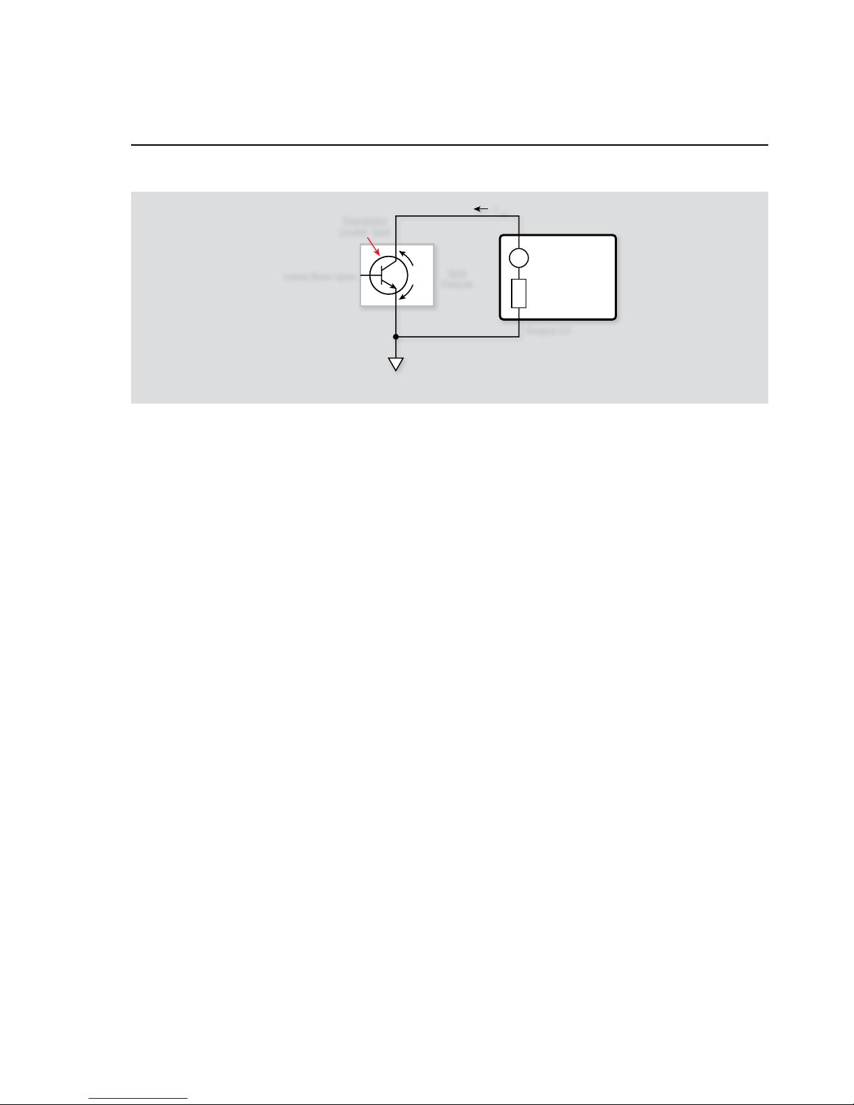
3-11

SECTION 3

Bipolar Transistor Tests

3.6.2 Example Program 8: I

CEO

Test

Use Program 8 to run I

CEO

tests on bipolar transistors. Follow

these steps to run the program:

With the power off, connect a dual-channel System Source-1. Meter instrument to the computer’s IEEE-488 interface.

Connect the test ﬁxture to both units using appropriate 2. c a b l e s .

Turn on the instrument and allow the unit to warm up for two 3. hours for rated accuracy.

You can simply copy and paste the code from Appendix A in 5. this guide into the TSB script editing window (Program 8), manually enter the code from the appendix, or import the TSP ﬁle ‘Iceo.tsp’ after downloading it to your PC.

If your computer is currently connected to the Internet, you can click on this link to begin downloading: http://www.

keithley.com/data?asset=50917.

Install a small-signal NPN silicon transistor such as a 2N3904 6. in the appropriate transistor socket of the test ﬁxture.

Once the code has been placed in the instrument run-time 8. memory, we can run it at any time simply by calling the function ‘

Iceo()

’. This can be done by typing the text ‘

Iceo()

’

after the active prompt in the Instrument Console line of TSB.

In the program ‘9. Iceo.tsp’, the function

Iceo(vstart,

vstop, vsteps)

is created.

vstart represents the initial voltage value in the V•

sweep

vstop represents the ﬁnal voltage value in the V•

sweep

vsteps represents the number of steps in the sweep•

If these values are left blank, the function will use the default values given to the variables, but you can specify each variable value by simply sending a number that is in-range in the function call. As an example, if you wanted to have the start voltage be 1V, the stop value be 11V, and the number of steps be 20, you would send

Iceo(1, 11, 20

) to the instrument.

The sources will be zeroed and then enabled. The program 10. will execute a voltage sweep on the collector-emitter and measure the collector-emitter current (I

CEO

) at each point.

Once the measurements have completed, the data (V11.

and ICE)

will be presented in the Instrument Console window of TSB.

3.6.3 Typical Program 8 Results

Figure 3-8 shows an example I

CEO

vs. V

CEO

plot generated by Program 8. The device used for this example was a 2N3904 NPN tr ansistor.

3.6.4 Program 8 Description

The instrument is returned to default conditions. SMUA, which sweeps V

CEO

and measures I

CEO

, is set up as follows:

Source V•

Local sense•

10mA compliance, autorange measure•

1 NPLC Line cycle integration•

Series 2600

System

SourceMeter

Channel A

Source V

CEO

Measure I

CEO

Test

Fixture

Transistor

Under Test

Leave Base open

Output LO

CEO

Figure 3-7. Conﬁguration for I

CEO

tests

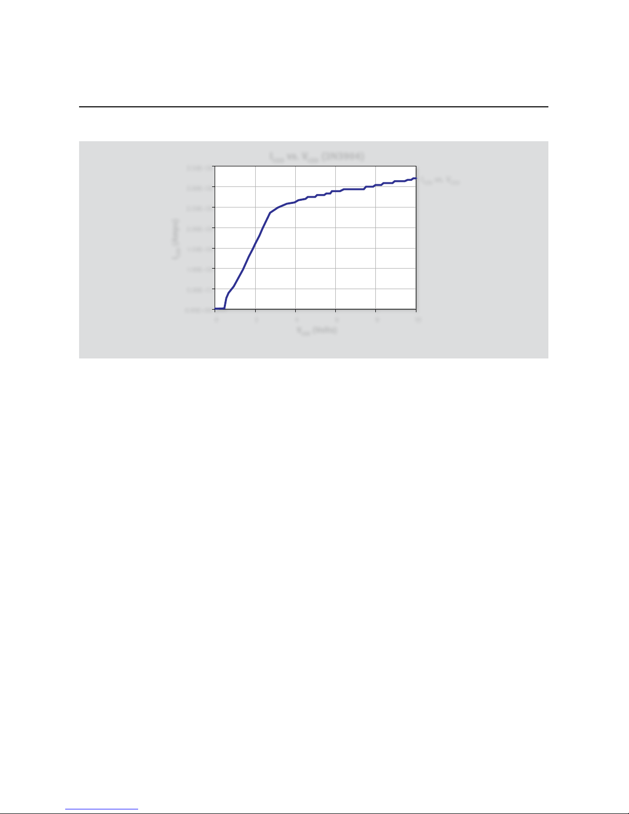
3-12

SECTION 3

Bipolar Transistor Tests

vstart

• : 0V

vstop

• : 10V

vsteps

• : 100

After setup, the output is zeroed and enabled. A linear voltage sweep from the start to the stop value is performed. At each step, the collector-emitter current (I

CEO

) is measured.

Upon sweep completion, the output is disabled and the data is written to the Instrument Console window of TSB.

3.6.5 Modifying Program 8

For different sweep values, simply modify the

vstart, vstop

and

vstep

values and source range parameter as appropriate.

In order to speed up the test procedure, you may wish to use a faster integration period. Simply change the

l _ nplc

value. Note, however, that changing this parameter may result in unacceptable reading noise.

CEO

vs. V

CEO

(2N3904)

CEO

(Volts)

CEO

vs. V

CEO

(Amps)

3.50E–10

3.00E–10

2.50E–10

2.00E–10

1.50E–10

1.00E–10

5.00E–11

0.00E+00

0 2 4 6 8 10

Figure 3-8. Program 8 results: I

CEO

vs. V

CEO

4-1

Section 4

FET Tests

4.1 Introduction

FET tests discussed in this section include tests to generate common-source characteristic curves, and transconductance tests. Example programs for each of these applications are also included.

4.2 Instrument Connections

Two SMU channels are required for the tests and a dual-channel instrument from the Series 2600 System SourceMeter line is recommended. A test ﬁxture with safety interlock is recommended for connections to the FET under test.

For general-purpose measurements with most of the Series 2600 instruments, Model 2600-BAN cables are recommended. For low current tests (<1mA) or when using a low current instrument like the Model 2636, Model 7078-TRX-3 triax cables are recommended to make instrument-to-test ﬁxture connections.

WAR NING Lethal voltages may be exposed when the test ﬁxture lid is open. To avoid a possible shock hazard, a safety interlock circuit must be connected before use. Connect the ﬁxture screw to safety earth ground using #18 AWG minimum wire before use. Turn off all power before connecting or disconnecting wires or cables

NOTES

Remote sensing connections are recommended for optimum accuracy. See paragraph 1.2.2 for details.

If measurement noise is a problem, or for critical, low level applications, use shielded cable for all signal connections.

4.3 Common-Source Characteristics

One of the more common FET tests involving family of curves is common-source characteristics. Such tests are very similar to the common-emitter characteristic tests outlined earlier except,

of course, for the fact that an FET rather than a bipolar transistor is involved.

Test data for common-source characteristics are obtained by sweeping the gate-source voltage (VGS) across the desired range of values at speciﬁc increments. At each VGS value, the drain-source voltage (VDS) is swept through the required range, once again at the desired increments. At each VDS value, the drain current (ID) is measured. Plots can then be made from this data to show ID vs. VDS with one curve for each value of VGS.

4.3.1 Test Conﬁguration

Figure 4-1 shows the test conﬁguration for the common-source tests. SMUB sweeps VGS, while SMUA sweeps VDS, and the instrument also measures ID. For this programming example, a smallsignal, N-channel FET such as a SD210 is recommended.

4.3.2 Example Program 9: Common-Source Characteristics

Program 9 outlines general programming techniques for measuring common-source characteristics. Follow these steps to use this program:

With the power off, connect a dual-channel System Source-1. Meter instrument to the computer’s IEEE-488 interface.

Connect the test ﬁxture to both units using appropriate 2. cables.

Turn on the instrument and allow the unit to warm up for two 3. hours for rated accuracy.

You can simply copy and paste the code from Appendix A in 5. this guide into the TSB script editing window (Program 9), manually enter the code from the appendix, or import the TSP ﬁle ‘FET_Comm_Source.tsp’ after downloading it to your PC.

If your computer is currently connected to the Internet, you can click on this link to begin downloading: http://www.

keithley.com/data?asset=50921.

+ 106 hidden pages

Keithley Series 2600 Application Manual

Specifications and Main Features

Frequently Asked Questions

User Manual