

Page 1

KD-5100
Instruction Manual
Differential Measuring Systems
DO NOT MAKE ANY MODIFICATIONS TO CABLE LENGTH, SENSOR OR
CALIBRATED TARGET MATERIALS WITHOUT PRIOR CONSULTATION WITH
A KAMAN APPLICATION ENGINEER
********
********
Copyright © 2000
PART NO: 860029-001
Rev. C
Page 2

KD-5100 SERIES
DIFFERENTIAL
MEASURING SYSTEM
INSTRUCTION MANUAL
P/N 860029-001 REVISION B
2
Page 3

CONTENTS
1. INTRODUCTION............................................................................................. 5
1-1. Calibration...............................................................................................................5
1-2. Maintainability........................................................................................................ 5
1-3. Environments ..........................................................................................................5
2. THEORY OF OPERATION..................................................................... 6
3. OPTIMUM PERFORMANCE.................................................................7
4. APPLICATION INFORMATION.......................................................... 8
5. TARGETS............................................................................................................ 9
5-1. Material ................................................................................................................... 9
5-2. Thickness ..............................................................................................................10
5-3. Size........................................................................................................................ 10
6. SPECIAL HANDLING CAUTIONS................................................. 10
6-1. The Sensors........................................................................................................... 10
6-2. The Mounting Surface ..........................................................................................11
7. FIXTURING....................................................................................................... 12
8. CROSS-AXIS SENSITIVITY................................................................ 15
9. PIN OUT and CONNECTOR ASSIGNEMENTS................... 17
10. USER’S ABBREVIATED FUNCTIONAL TEST.................. 18
11. SENSOR INSTALLATION GUIDELINES AND
PROCEDURES
..................................................................................................... 19
12. CALIBRATION............................................................................................ 20
12-1. Pitfalls: ................................................................................................................ 20
12-1a. Dimensional Standard: .................................................................................. 20
12-1b. Recalibration ................................................................................................. 20
12-1c. Thermal Equilibrium..................................................................................... 20
12-2. Equipment Needed to Calibrate:......................................................................... 22
12-3. Calibration Procedure Overview: ....................................................................... 22
12-4. Calibration Steps:................................................................................................ 22
13. TROUBLESHOOTING.......................................................................... 24
14. TERMINOLOGY......................................................................................... 26
TOTAL SYSTEM SPECIFICATIONS*................................................. 28
PERFORMANCE ......................................................................................................... 28
ELECTRICAL ..............................................................................................................28
TEMPERATURE.......................................................................................................... 28
MICRO-CONVERSION SC ALE................................................................ 29
DIGITAL DYNAMIC RANGE........................................................................................ 29
CUSTOMER SERVICE INFORMATION ……………………………30
TECH NOTES…………………………………………………………………….31
3
Page 4

ILLUSTRATIONS
Figure 1 Block Diagram: Differential Measuring System .................................................6
Figure 2 Sensor and Target Geometry ................................................................................7
Figure 3 Differential Target Configurations .......................................................................8
Figure 4 x-y Mirror Alignment Configuration.................................................................... 9
Figure 5 Aluminum Targets on Invar.................................................................................. 9
Figure 6 Mounting/Cover Plate Dimensions..................................................................... 11
Figure 7 15N Sensor Dimensions ..................................................................................... 13
Figure 8 20N Sensor Dimensions ..................................................................................... 14
Figure 9 Sensor Coil Dimensions ..................................................................................... 15
Figure 10 Sensor Cable Connections ................................................................................ 17
Figure 11 Power & Output Connections ........................................................................... 17
Figure 12 Sensor Field ......................................................................................................19
Figure 13 Calibration Cover Dimensions ......................................................................... 21
Figure 14 Zero & Gain Control Location Case Dimensions............................................ 23
Figure 15 Null Gap, Offset, Measuring Range .................................................................26
4
Page 5

KD-5100 SERIES
DIFFERENTIAL MEASURING SYSTEMS
INSTRUCTION MANUAL
YOUR SYSTEM’S SPECIFICATIONS:
Sensor Type __________ Null Gap __________
Offset __________ Measuring Range __________
Full Scale Output __________ Scale Factor __________
Target Material __________
1. INTRODUCTION
This manual describes installation and use of the KD-5100, theory of operation, ways to optimize
performance, special handling cautions, functional tests, and guidelines for fixturing and targets,
and calibration procedures.
1-1. Calibration
Though there is a section on calibration, these systems are shipped from the factory calibrated for
a user specified target, sensitivity, and measuring range. We calibrate these systems in a
controlled environment using a precision laser as a primary dimensional standard. Since it is
difficult for users to duplicate our calibration conditions, call us before attempting any
adjustments of your KD-5100. On the other hand, it is equally difficult for Kaman to duplicate
your actual application conditions, so special circumstances may dictate come calibration.
Again, coordinate with a Kaman engineer first.
1-2. Maintainability
The KD-5100 is designed so scheduled maintenance and adjustments are not required. The unit
can be removed and replaced without special tools.
1-3. Environments
The KD-5100 provides specified performance after exposure to all natural and/or induced
environments encountered during manufacture, test, transportation, handling, storage,
installation, and removal operations.
5
Page 6
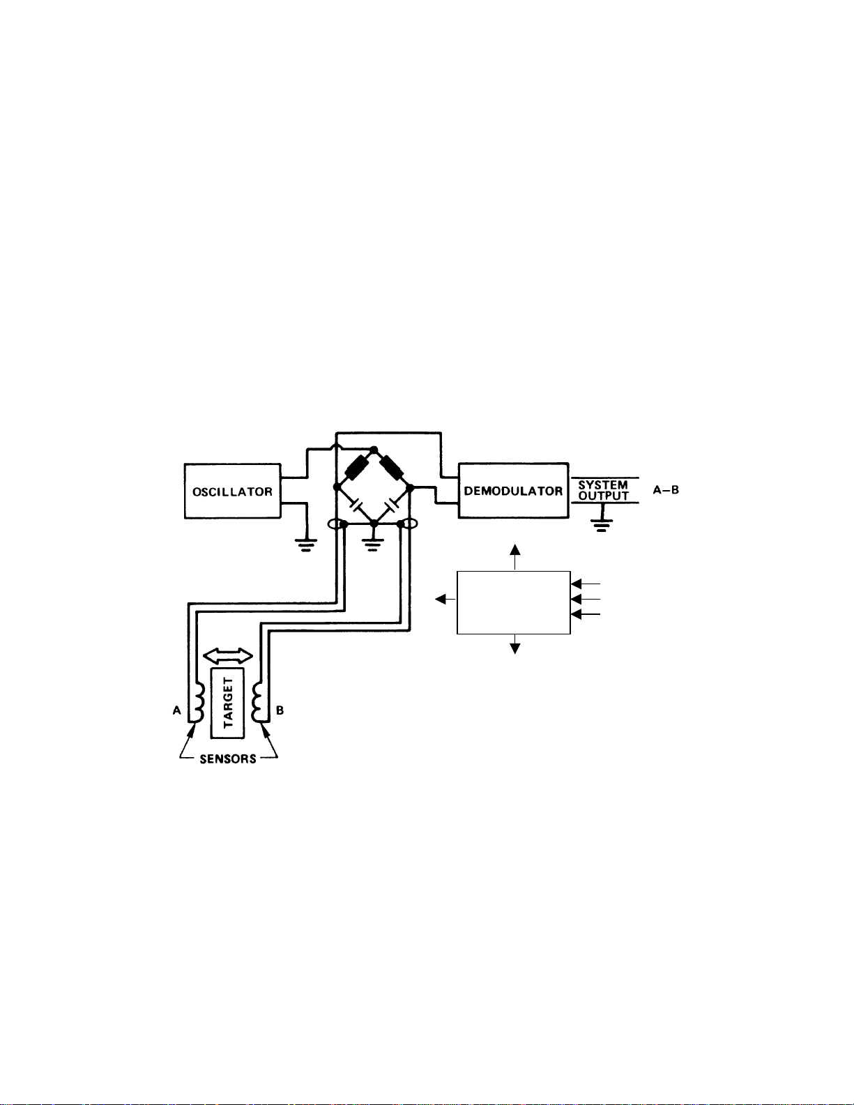
2. THEORY OF OPERATION
2-1. The KD-5100 Differential Measuring System uses advanced inductive measurement
technology to detect the aligned or centered position of a conductive target. Two matched
sensors are positioned relative to the target so that as it moves away from one sensor it moves
toward the other an equal amount.
2-2. The transducer operates on the principle of impedance variation caused by eddy currents
induced in a conductive target located within range of each sensor. The coil in the sensor is
energized with an AC current, causing a magnetic coupling between the sensor coil and the
target. The strength of this coupling depends upon the gap between them and changes in gap
cause an impedance variation in the coil.
2-3. In the KD-5100, the coils of a pair of sensors form the opposite legs of a balanced bridge
circuit (Figure 1).
VOLTAGE
REGULATOR
+15 Vdc
COMMON
-15 Vdc
Figure 1 Block Diagram: Differential Measuring System
2-4. When the target is electrically centered between the two sensors at the nominal null gap for
each, the system output is zero. As the target moves away from one sensor and toward another,
the coupling between each sensor and target is no longer equal causing an impedance imbalance
between the sensors. The bridge detects this imbalance and its output is amplified, demodulated,
and presented as a linear analog signal directly proportional to the targets position. This is a
bipolar signal that provides both magnitude and direction of misalignment. Only the differential
output is available.
6
Page 7
2-5. This differential configuration achieves its high resolution by eliminating the noise and drift
any intervening summation and Log amplifiers normally add to the system.
2-6. Maximum performance depends upon advanced sensor technology. Factors critical to the
high resolution of the KD-5100 are tighter manufacturing control, using significantly larger coils
for a given range of operation, and electrically matching the sensors.
2-7. By using electrically matched sensors on opposing legs of the same bridge, temperature
effects common to the sensors and cabling of a differential sensor pair tend to be cancelled. This
is true for the mechanical aspects of the sensor/target system also. Assuming the thermal
characteristics of each sensor track together, slight changes in sensor length due to temperature
tend to be cancelled.
3. OPTIMUM PERFORMANCE
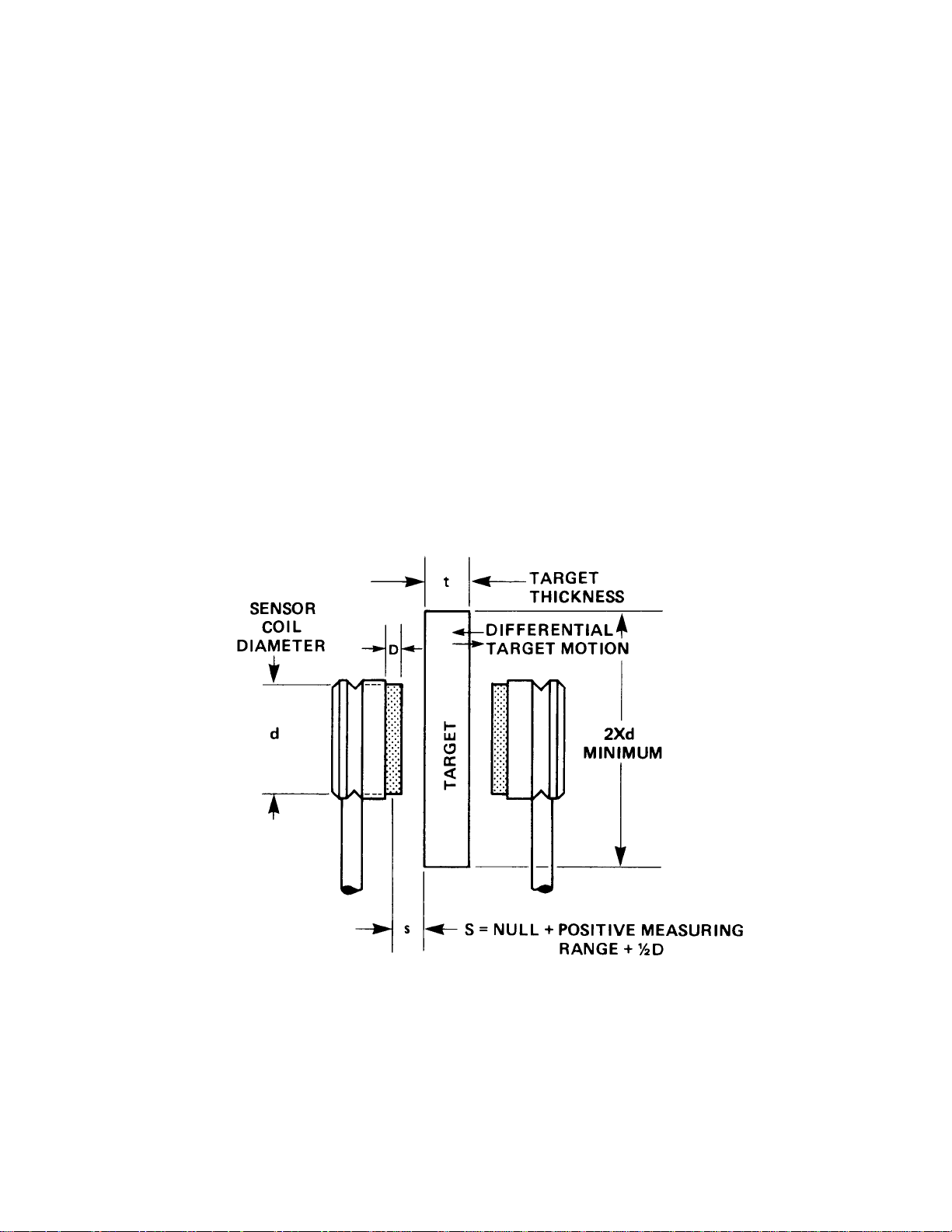
3-1. To optimize the performance of a KD-5100 system, a high (d) to (s) ration is desired: (d) is
the sensor coil diameter and (s) includes: the null gap, the positive measuring range, and ½ of
the coil depth (Figure 2).
Figure 2 Sensor and Target Geometry
3-2. The 15N sensor used over the specified ±0.009” measuring range provides a d/s ration of
3.08. The ration for the 20N is 10.68. Therefore, if mounting space and target size permit, the
20N offers better performance over the specified measuring range.
7
Page 8
3-3. For either sensor model, performance can be improved by decreasing the one variable, the
measuring range. Significant reduction can provide a d/s ration up to 35. This effectively lowers
the noise floor and improves resolution, linearity, and thermal stability.
3-4. The temperature of the mounting surface and the environment for the electronics should not
exceed the specified –20
o
C to 60oC (-4oF to +140
o
F). For optimum performance, stabilize the
temperature for the mounting surface/electronics at a constant temperature within this range,
preferably 25
o
C.
4. APPLICATION INFORMATION
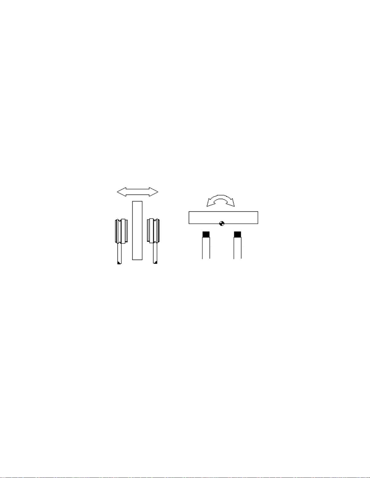
4-1. For differential measurement applications, the two electronically matched sensors are
positioned on opposite sides or ends of the target (Figure 3). The sensor to target relationship is
such that as the target moves away from one sensor, it moves toward the other an equal amount.
Figure 3 Differential Target Configurations
4-2. A standard system comes with two measurement axes (four sensors – two per axis) and can
therefore be fixtured a number of ways to provide precise x-y alignment. Figure 4 illustrates
target configuration for x-y alignment of an image stabilization mirror for an electro-optical
application.
8
Page 9
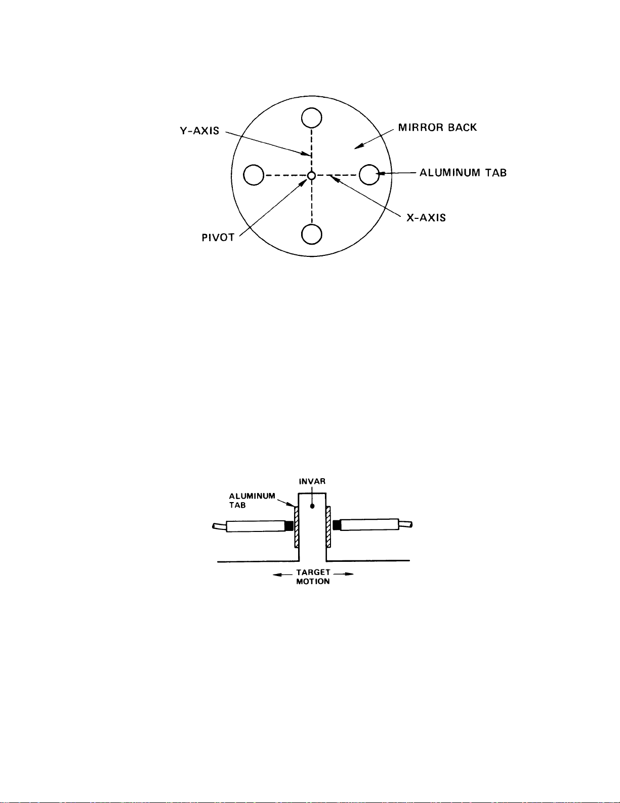
Figure 4 x-y Mirror Alignment Configuration
5. TARGETS
5-1. Material
5-1a. Iron, nickel, and many of their alloys (magnetic targets) are not acceptable for use with the
KD-5100.
5-1b. Aluminum is preferred as the most practical target material. You can mount aluminum
targets on materials with more stable temperature characteristics such as Invar or other substrates
as long as target thickness guidelines are observed (Figure 5).
Figure 5 Aluminum Targets on Invar
5-1c. These systems are set up to work with other nonmagnetic conductive targets on a special
order basis. If you purchased a system for use with a target material other than aluminum, it has
been calibrated (with selected component values) at the factory using that target material. An
arbitrary change in target material may, at a minimum, require calibration or, not work at all.
9
Page 10

5-2. Thickness
5-2a. The RF field developed by the sensor is at a maximum on the target surface. There is
penetration below the surface and the extent of penetration is a function of target resistivity and
permeability. The RF field will penetrate aluminum to a depth of 0.022”, a little more than three
“skin depths” (at one skin depth the field density is only 36% of surface density and at two skin
depths it is 13%). To avoid variations caused by temperature changes of the target, the minimum
thickness should be at least three skin depths.
5-2.b The depth of penetration depends on the actual target material used (Table 1). In cases
where the sensors are opposing each other, aluminum target thickness must be at least 0.050” to
prevent sensor interaction.
Table 1 Recommended minimum target thickness in mils.
Material Thickness in mils
Silver and Copper 11-13
Gold and Aluminum 13-18
Beryllium 17
Magnesium, Brass, Bronze, Lead 26-39
300 Series Stainless 75
Inconel 95
5-3. Size
The minimum target cross section must be 1½ to 2 times sensor diameter.
6. SPECIAL HANDLING CAUTIONS
6-1. The Sensors
Due to design requirements, the sensor’s most critical component, the coil, is exposed. We ship
the sensors with protective caps. Keep them in place until installation of the sensors.
CAUTION: If any sharp object comes in contact with the coil face or edge and
damages it in any way, this could short a number of turns in the coil, alter its
impedance, and render it useless.
10
Page 11
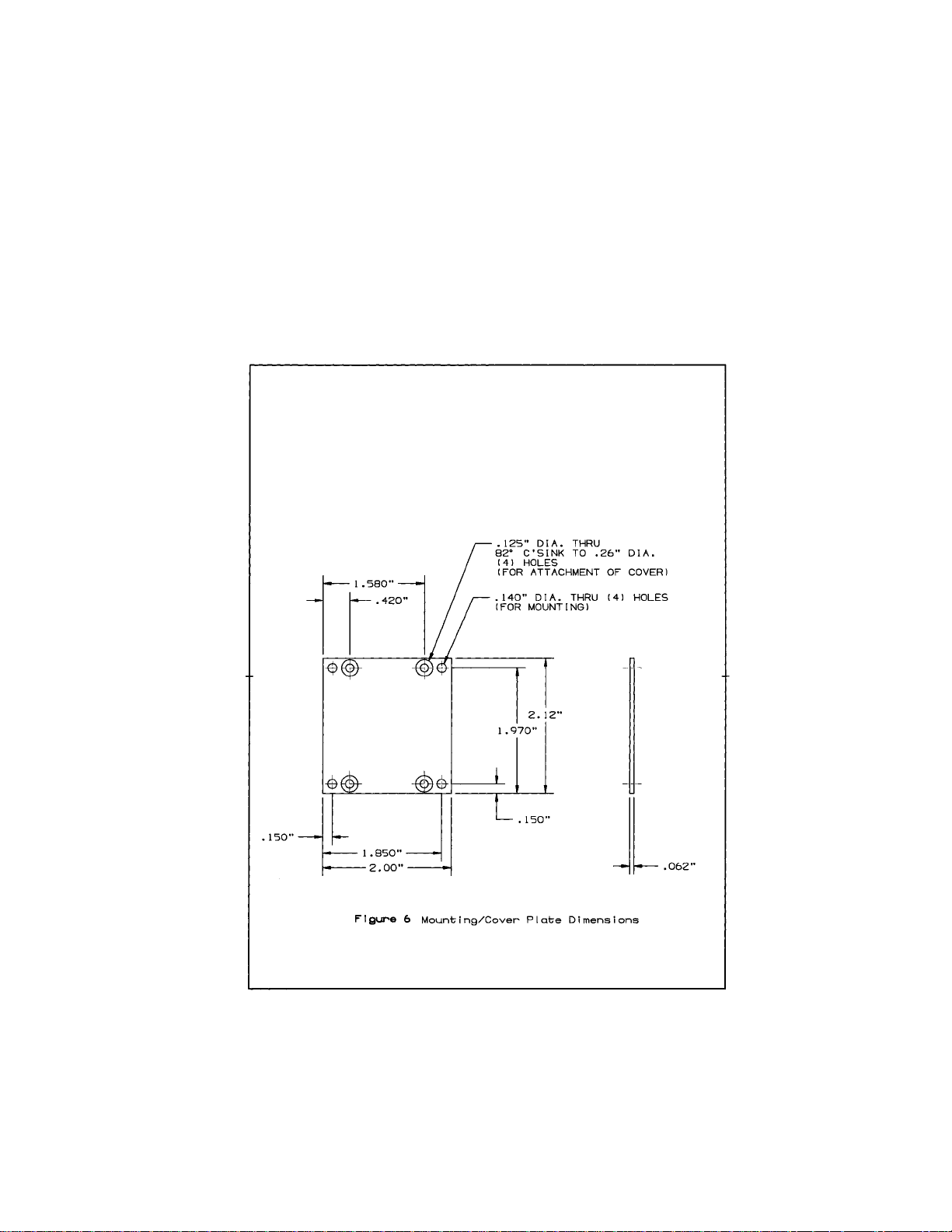
6-2. The Mounting Surface
The base plate of the electronics module has a smooth surface to enhance thermal conduction
away from the electronics. Mounting the base plate flush with another surface will enhance
thermal dissipation (assuming a mount surface with a temperature below 60
dimensions and mounting hole spacing are shown in Figure 6.
o
C). Base plate
Figure 6 Mounting/Cover Plate Dimensions
11
Page 12

7. FIXTURING
7-1. The user provides fixturing for the KD-5100 electronics and sensors. The following
information establishes fixturing requirements for optimum system performance. The quality of
the measurement is both a function of Kaman’s system and your Fixturing.
7-2. Both the sensor and target fixturing must be structurally sound and repeatable.
7-3. Factors that degrade performance are:
7-3a. Unequal Loading
This refers to an unequal amount of conductive material within the field of one sensor of
a pair as opposed to another (the sensor’s field is approximately three times its diameter).
Unequal loading causes asymmetrical output from the sensor, which induces nonlinearity in the system output. Ideally, no conductive material other than the target
should be in the sensor’s field. Some loading may be acceptable if it is equal and the
sensors are calibrated in place. Even then, sensor loading may cause non-linearity. If
unable to calibrate – loading is too great.
7-3b. Unequal Displacement
For targets using a pivot point mount (examples, Figures 3 & 4) the system should “see”
equal displacement: i.e., the pivot point of the target is perfectly centered between the
sensors. If the pivot point is a fraction of a mil off it can introduce non-linearity into the
system.
7-4. Other pivot point requirements:
7-4a. The pivot point must be a common line between the centerline of a pair of sensors.
7-4b. The axis of tilt must be a perpendicular bisector of a line between the centerlines of
a sensor pair.
7-4c. The pivot point must be positioned on the target so as not to introduce a translation
error. This error, a function of angle, is caused by slight changes in the effective null gap
as the target moves about the pivot. This results in non-linearity.
7-4d. The pivot point must not change or move with time.
7-5. Sensor mounting considerations:
7-5a. The sensors must be securely clamped. Sensor dimensions are shown in Figures 7
and 8.
12
Page 13
Figure 7 15N Sensor Dimensions
13
Page 14

Figure 8 20N Sensor Dimensions
7-5b. The target must not strike the sensor face. This system has a null gap of 15 mils
(0.015”/0.381mm) for the 15N sensor and 20 mils (0.020”/0.508mm) for the 20N sensor.
The specified full measuring range for both sensors is ±0.009” (±0.228mm). The
difference between the null gap and measuring range (6 mils for the 15N and 11 mils for
the 20N) is the offset distance for the sensors. This offset is necessary both to optimize
performance and to keep the target from contacting and possibly damaging the coils in
the sensor face.
7-5c. The sensor coil is mounted at the face of both sensors. For purposes of mechanical
nulling, measure distance from the sensor face. (For electrical nulling, the most accurate
method, the null gap is referenced to the electrical centerline, which is one half of the coil
depth – ½D, Figure 9.)
14
Page 15

15N 20N
Figure 9 Sensor Coil Dimensions
7.5d. If the face of the sensor and the target surface are not parallel (if the sensor
centerline is not perpendicular to the target) more than 2
o
to 3o, it will introduce error to
the measurement.
8. CROSS-AXIS SENSITIVITY
8-1. Assuming you have stable and repeatable fixturing, and have followed all of the rules for
target mounting, pivot points, etc., under certain conditions the system may exhibit signs of error
we classify as cross-axis sensitivity.
8-2. Cross-axis sensitivity may occur under the following conditions:
8-2a. The target must be one with x and y axes of tilt moving about a central pivot point
(see Figure 4). When the target tilts full range in its x axis, it should be able to tilt full
range in its y axis without any change in the indicated output of the x axis (or vice versa).
This may not be the case. Cross-axis tilt can increase the coupling between the sensor
and target, which causes a slight change in output, though there is no change in the actual
distance between the sensor and target. This is a definition of error.
8-2b. This error manifests itself as increased non-linearity of the output at the extreme
end points of target travel only. (This non-linearity can change overall linearity from the
specified 0.1% to about 0.3%.)
8-3. Additional points of emphasis about cross-axis sensitivity:
8-3a. Again, the error manifests itself only at the end points of target travel (the last
20%) when the target tilts fully in both x and y axes.
15
Page 16

8-3b. The degree of error is related to the angle between the sensor and target face. As a
general rule, for angles ± 1o or less, there is virtually no problem with cross-axis
sensitivity.
Sensor/target angle is a function of the distance between the sensor and target pivot,
and the measuring range. A sensor with a range of ± 10 mils mounted 10 mils from
the pivot will experience 45o of tilt at the end points. This is an extreme example but
suffices to illustrate the point. A sensor with a ± 10 mil range must be mounted
approximately 550 mils (13.9mm – a little over ½ inch) from the pivot to achieve a 1
o
angle between sensor and target.
8-3c. This phenomenon is related to basic physics and is stable, repeatable, small in
magnitude, and can therefore be characterized. If necessary, users can provide a
computer correction scheme.
8-4. Cross-axis sensitivity is not a problem for the majority of applications. If you anticipate or
experience the problem, contact Kaman Instrumentation for test data, which specifies under
which conditions and to what degree cross-axis sensitivity exists.
16
Page 17

9. PIN OUT and CONNECTOR ASSIGNEMENTS
9-1. Sensor cable connections (Figure 10):
AXIS CONNECTORS SENSORS
1 J3 J1 S3 S1
2 J4 J2 S4 S2
Figure 10 Sensor Cable Connections
9-2. Pin assignments for the Power/Signal line connector J5 (Figure 11):
PIN FUNCTION
1 + 15Vdc*
2 - 15 Vdc*
3 Power Supply Common
4 Signal Output: Axis 1
5 Return Signal for Pin 4
6 Signal Output: Axis 2
7 Return Signal for Pin 6
8 Not Used
9 Not Used
*Power Requirements Tolerance
+ 15Vdc +1.0, -0.5Vdc
- 15 Vdc +0.5, -1.0Vdc
Figure 11 Power & Output Connections
17
Page 18

10. USER’S ABBREVIATED FUNCTIONAL TEST
NOTE: This is not a calibration or installation procedure. This unit is factory calibrated,
and installation guidelines are in the next section. This is simply a check to make sure
your system is functioning upon receipt.
10-1. Procedures
Perform this abbreviated functional test prior to installation of the electronics and sensors in the
application fixture.
10-1a. Attach the power supply cable to connector J5 and apply power to the system.
10-1b. While monitoring the system output, place an aluminum target within 0.015”
(15N sensor) or 0.020” (20N sensor) of sensor S3. It is preferable this step be
accomplished using a fixture to hold the sensor and to control target movement.
However, carefully hand holding and moving the sensor or the target will be sufficient
for this check. (See Figure 11 for power and output connections at J5. The output for
sensor S3 and S1 [axis 1] is at pin 4.)
10-1c. Slowly move the target through the sensor’s measuring range to check for a full
range of output for S3: 0Vdc to +9Vdc.
10-1d. Next: Check S1 for 0Vdc to –9Vdc.
Note: This will not be a linear output and you may get an output with the sensor
as much as 15 or 20 mils away from its target. That is OK since this check is only
to confirm that the system is working.
10-1e. Repeat the above test for sensor S4 @ +9Vdc and S2 @ -9Vdc. Axis 2 output is
pin 6.
10-2. If the output does not change during this test:
10-2a. Make sure you have power applied at the correct voltage: +14.5 to 16Vdc and
–14.5 to –16Vdc.
10-2b. Make sure the wiring to connector J5 is correct (see Figure 11).
10-2c. Make sure you are monitoring the correct channel for the sensor you are
checking: S3 & S1 = axis 1 (pin 4), S4 & S2 = axis 2 (pin 6).
Still no change: return the unit to Kaman Instrumentation for servicing.
18
Page 19
11. SENSOR INSTALLATION GUIDELINES AND PROCEDURES
11-1. The electrical nulling procedure.
Note: This installation procedure is the preferred method. Though both sensors may be
positioned mechanically, this can cause a cumulative error. By electrically positioning
the second sensor of a pair using system output, any existing error is self-canceling.
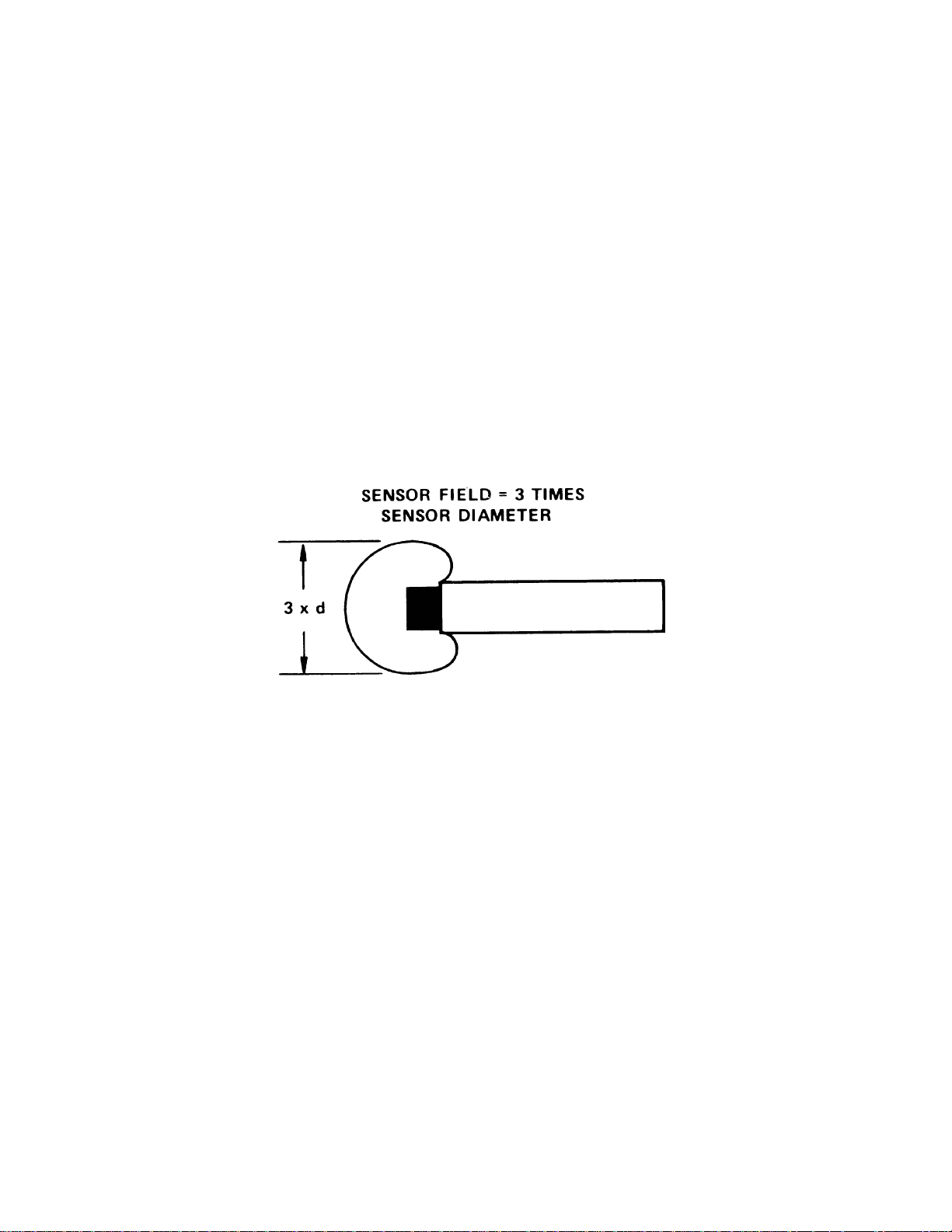
11-2. Install the sensors so that only the target interacts with the sensor’s field. This means no
conductive material other than the target within a circle around the sensor that is three times the
sensor’s diameter. The sensor field radiates in all directions. (Figure 12) and excessive back
loading can also be a problem.
CAUTION: Be sure not to damage the sensor coil during this procedure
Figure 12 Sensor Field
11-2a. This procedure assumes the electronics are installed in the application fixture.
11-2b. The sensor coil is mounted at the face of both sensors. For purposes of
mechanical nulling, measure distance from the sensor face. For electrical nulling the null
gap is referenced to the electrical centerline, which is one half of the coil depth (½D,
Figure 9).
11-3. Sensor position relative to the target is critical. Make sure the target is in the null position.
Install the first sensor of a pair (start with S3) in the application fixture. Using a dimensional
standard, precisely locate the sensor 15 mils (±0.2 mils) for the 15N sensor, or 20 mils (±0.2
mils) for the 20N sensor from the target. Secure the sensor and recheck its position.
11-4. Now install the second sensor of the pair (S1) in the fixture and position it to within a few
mils of the required null gap. Connect the Power/Signal line to J5 and apply power to the
system. Use the output from the system as a guide in the final positioning of this sensor
(electrical nulling). Slowly move the second sensor toward or away from the target as necessary
19
Page 20

until the system output reads 0Vdc (ideally, 0.000 volts). This output means the sensor is
positioned correctly.
11-5. Repeat steps 11-3 and 11-4 for sensor S4 and S2.
11-6. The system is now ready to use.
12. CALIBRATION
12-a. These systems are shipped from the factory pre-calibrated for a user specified
measuring range, sensitivity, and target material. They do not normally require
calibration or re-calibration. Yet some applications dictate the availability of this option.
12-b. The calibration procedure is very simple. The problems arise in finding an
accurate enough dimensional standard and a stable environment.
Therefore, there are some pitfalls…
12-1. Pitfalls:
12-1a. Dimensional Standard:
To calibrate, you need some dimensional standard (a micrometer, laser interferometer, a
weight to provide a known deflection, etc.). This should be a standard that you believe in
and know to be accurate and repeatable. Whether you are measuring in mils, microns,
micro-radians, or whatever, you must have a means of accurately positioning the target,
using the dimensional standard, to the desired measurement units.
Kaman Instrumentation uses a laser interferometer as a primary dimensional standard for
calibration.
12-1b. Recalibration
Recalibration to a sensitivity and/or measuring range significantly different from the
factory calibration may not be possible. For example, if you purchased a standard system
calibrated 0 to 9 volts over a 9 mil measuring range (1V/mil) and attempted to recalibrate
for 9 volts over a 3 mil measuring range (3V/mil) there may not be sufficient gain
adjustment to do this. These units are built with component values selected for each
application. Therefore, changes in measuring range, sensitivity, or target material may
not be possible and will require reconfiguration by Kaman Instrumentation.
12-1c. Thermal Equilibrium
The mounting/cover plate helps maintain thermal equilibrium inside the module and acts
as a heat sink for the hybrid circuit. The hybrid has two watts of power to it and needs
20
Page 21

the cover plate for heat sinking. The calibration controls are located inside the unit and
the cover plate must be removed to access them. Removing the cover plate removes its
heat sinking function. Calibrating with the cover off and then reinstalling it will cause
enough of a thermal gradient to throw the calibration off.
12-1c1. Kaman’s solution is to use a cover plate with holes drilled in it for access to
the calibration controls. This plate is available as an accessory from Kaman. The
factory installed cover plate has a mica insulator epoxied to the inside with silicon
heat sink compound between the mica and the hybrid housing.
12-1c2. You may either obtain a calibration cover plate from Kaman or fabricate one
from 0.062” thick aluminum. Dimensions and location of the holes are shown in
Figure 12. Use a double thick layer of Sil-pad as an insulator. Although the heat sink
properties of the Sil-pad are not as good as the mica/heat sink compound, it is
adequate for calibration purposes. The hybrid is recessed in the case, this is why we
recommend two layers of Sil-pad, to ensure contact and thermal conductivity.
Figure 13 Calibration Cover Dimensions
(see page 11 for additional cover plate dimensions)
21
Page 22

12-2. Equipment Needed to Calibrate:
1. A dimensional standard
2. A regulated ± 15 Vdc power supply
3. A voltmeter accurate to one millivolt
4. An insulated adjusting tool (“tweaker”) Kaman P/N 823977-T007
5. A calibration cover plate
NOTE: When you do a system calibration, if at all possible, do it with the system
installed in the application fixture at normal operating temperatures. This eliminates
any sift in system output caused by moving the system from a calibration fixture to
the application fixture (translation error).
12-3. Calibration Procedure Overview:
12.3a. Calibration involves five steps:
1. Null the Target
2. Monitor the output of axis 1 - Adjust for 0.000 volts output
3. Move the target to full displacement – Adjust for full output voltage
4. Return the target to the null position and check for an output of 0V±10mV
5. Repeat for axis 2
The following information details these five steps.
12-4. Calibration Steps:
12-4a. Install the sensors in the application fixture (or calibration fixture) and accurately
establish the null position for the target (see paragraph 11-3).
WARNING: Avoid contacting the eyes with silicone heat sink compound. It will
cause temporary irritation. It also stains clothing.
12-4b. Withdraw the four screws securing the cover plate and remove it. Silicone heat
sink compound has been liberally spread between the mica pad and the hybrid case.
12-4c. Install the calibration cover plate, power up the system and allow a 20 minute
warm-up period. Monitor system output.
22
Page 23
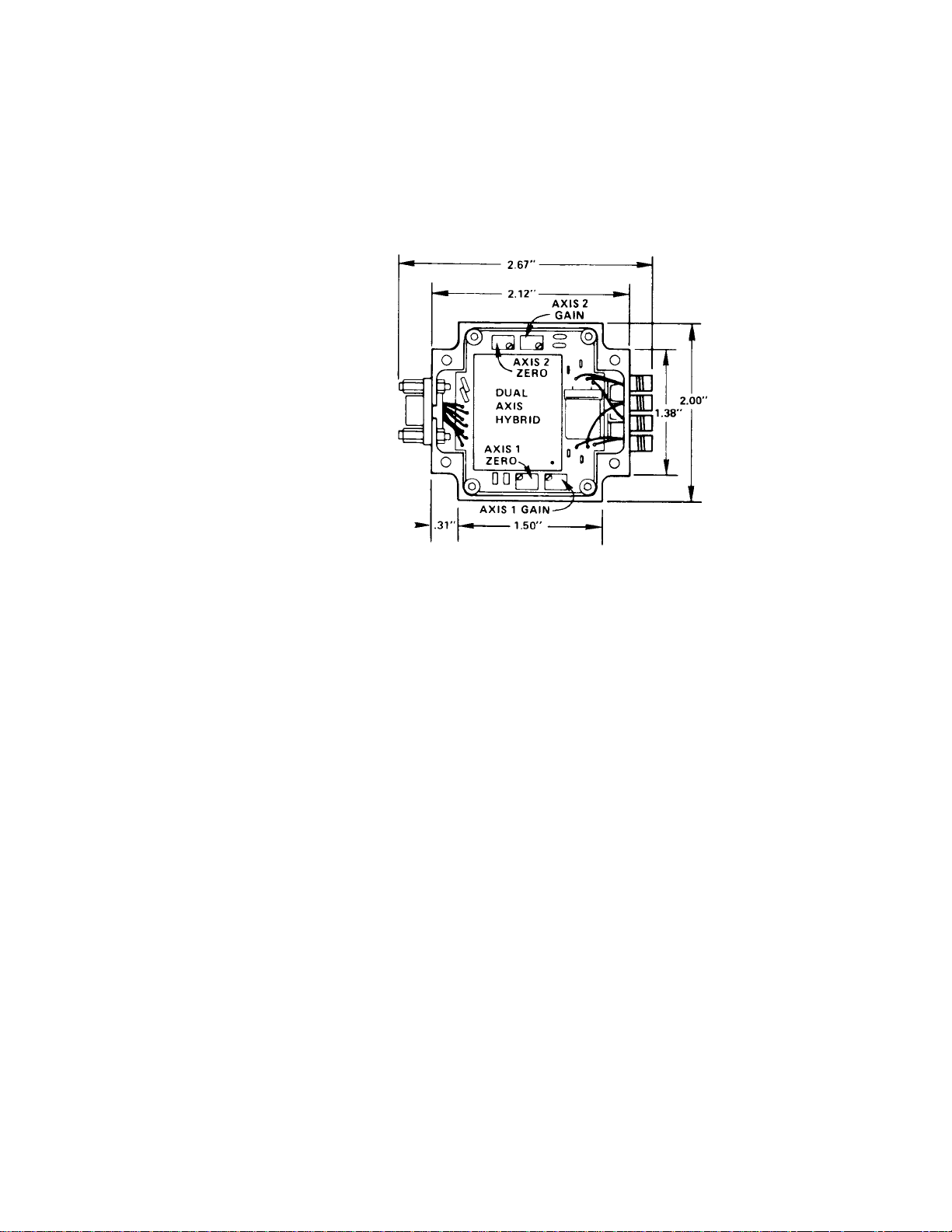
12-4d. To adjust for 0.000 volts:
1) Monitor the output of axis 1.
2) Using the adjusting tool, adjust the zero control for axis 1 (Figure 13) for 0.000
volts output.
Figure 14 Zero & Gain Control Location Case Dimensions
12-4e. Move the target through a known displacement to its maximum range (9 mils
standard) and adjust the axis 1 gain control (Figure 14) for the desired output (9 volts
standard).
12-4f. Return the target to the null position and check the output. You most likely will
not see 0.000 volts output unless you have a very good dimensional standard and very
stable fixturing located in a controlled environment. When measuring at sub micro inch
levels, the world becomes rubber, and your fixturing may have expanded or contracted
and you won’t see 0.000V again.
12-4f1. All things considered, after returning the target to the null position, output should
be 0V (±10mV or less). If the output at null exceeds this, repeat the process. Calibration
should not take more than two iterations.
12-4g. Repeat the process for axis 2, monitoring the output at pin 6.
12-4h. The system is ready to use.
23
Page 24

13. TROUBLESHOOTING
13-a. What if the above calibration process doesn’t work, if there is not enough gain for
the desired output, or if you cannot get a consistent 0V±10mV?
13-1. Insufficient Gain
13-1a. To repeat, if attempting to recalibrate for a sensitivity, measuring range, or target
different from factory calibration specifications, there may be insufficient gain control.
Another cause for insufficient gain could be excessive loading of the sensors by
conductive material (other than the target) within the field of the sensors. The sensor’s
field is approximately three times its diameter.
13-2. Can’t Zero
13-2a. The KD-5100 is an extremely stable measuring system- long term drift is less
than 2 micro inches per month. If the unit does not work, this would most likely be
discovered during the Abbreviated Function Test, Section J. Our experience in hundreds
of applications over years of use is that these systems either work or don’t, and are not
subject to “quirky” or “drifty” behavior. If you are unable to calibrate your system in no
more than two iterations, the problem is most likely poor mechanical repeatability in the
fixturing or actuating mechanisms.
13-3. There is a way to check it out:
Step 1. Do not make any adjustments to the calibration controls. Record how much time
the next step takes.
Step 2. Do at least 12 to 15 iterations of moving the target from null to full range and
back to null. Record the output at null each time. If successive readings of the output at
null constantly very with no clear trend (drift) in one direction or the other, the problem is
mechanical repeatability.
Step 3. Now, stabilize the target at null and record the output. Leave the target at null for
the same length of time it took to accomplish step two and monitor the output.
a. If the output remains constant, this confirms the problem was mechanical
repeatability.
b. If the output drifts, the problem could be:
(1) drift in the fixturing
(2) drift in the target positioning servos
(3) drift in the KD-5100
13-3a. If you can positively eliminate all other variables as the source of the problem,
return the KD-5100 to Kaman. Remember, if you are unable to calibrate the KD-5100
24
Page 25

and it passed the Abbreviated Function Test, it is the least likely candidate as the source
of the problem.
25
Page 26
14. TERMINOLOGY
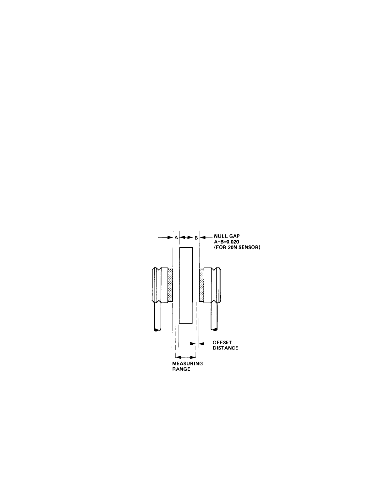
NULL GAP
The null gap is the point at which a target is equidistant from each sensor of a differential
pair. The system output at null = 0Vdc. The actual gap is measured from the sensor face
to the corresponding target face and includes a required offset (null gap = offset plus
maximum measuring range).
OFFSET
The offset is the minimum distance between the sensor face and the target. Offset is
necessary to prevent the target from striking the sensor face and to optimize performance
(offset = null gap minus max range).
MEASURING RANGE
The measuring range is the full range of target motion over which the various
specifications such as resolution, linearity, and sensitivity can be met. The differential
sensor arrangement yields a bipolar output and measuring range is expressed as a + and –
value either side of the null position (measuring range = null gap minus the offset).
SENSITIVITY
Sensitivity is the output voltage per unit of displacement. Usually expressed as millivolts
per mil (0.001”) or per millimeter.
Figure 15 Null Gap, Offset, Measuring Range
26
Page 27

LINEARITY
Linearity is the maximum deviation of any point of a calibrated system’s output from a
best-fit straight line. Express in actual units, e.g., microinches.
EQUIVALENT RMS INPUT NOISE
Equivalent RMS Input Noise is a figure of merit used to quantify the noise contributed by
a system component. It incorporates into a single value, several factors that influence a
noise specification such as signal-to-noise ration, noise floor, and system bandwidth.
Given a measuring systems sensitivity/scale factor and the level of “white” noise in the
system, Equivalent RMS Input Noise can be expressed using actual measurement units.
EFFECTIVE RESOLUTION
Effective Resolution is an application dependant value determined by multiplying the
Equivalent RMS Input Noise specification by the square root of the measurement
bandwidth.
Example: An application with a 100Hz bandwidth using a KD-5100 with an Equivalent
RMS Input Noise level of 0.2nm/ √Hz results in a system with an effective resolution of
0.2nm/ √Hz x √100Hz or 2 nanometers.
27
Page 28

TOTAL SYSTEM SPECIFICATIONS*
(sensor, cable, and electronics)
PERFORMANCE (typical for stated measurement conditions)
English (inches) Metric (mm)
Null Gap
KD-5100-15N 0.015±0.0001 0.381±0.003
KD-5100-20N 0.020±0.0001 0.508±0.003
Measuring Range
KD-5100-15N ±0.009 ±0.2286
KD-5100-20N ±0.009 ±0.2286
Sensitivity or scale factor 1V/0.001±2% 40mV/0.001±2%
Non-Linearity
KD-5100-15N ±2 x 10
KD-5100-20N ±1 x 20-5 ±2.5 x 10
Long Term Stability
Stabilized at 70
o
F (21oC) 5 x 10⁻⁶/month 1.27 x 10⁻⁴/month
Thermal Sensitivity at Null
(-20
o
F to 165oF)
KD-5100-15N <5 x 10
KD-5100-20N <5 x 10
Frequency Response ** DC to 5KHz
Equivalent RMS Input
Noise (DC to 5KHz) 4 x 10
Effective Resolution Equivalent RMS
Input noise x √bandwidth (Hz)
-5
±0.5 x 10
-6/o
F <2.3 x 10⁻⁴/oC
-6/o
F <2.3 x 10⁻⁴/oC
-9
/ √Hz max. 1 x 10⁻⁷/ √Hz max.
-3
-4
ELECTRICAL
Input Voltage ±15 Vdc @ 70mA Typical
Power Consumption (system) <2 Watts
Power Dissipation (15N sensors) <10 microwatts per Sensor
(20N sensors) <50 microwatts per Sensor
Output Characteristics <5 ohms @ 5mA
TEMPERATURE
Electronics: -4oF to 140oF (-20oC to 60oC)
Sensors: 15N: -62
20N: -62
20N (cryogenic): 4
WEIGHT (Electronics): 4 oz./113gr.
*Typical for an aluminum target
** Bandwidth limited to 22KHz ±5%
o
F to 220oF (-55oC to 105oC)
o
F to 220ooF (-55oC to 105oC)
o
Kelvin
28
Page 29

MICRO-CONVERSION SCALE
ENGLISH TO METRIC CONVERSIONS (0.001” = 1 mil = 25.4 mm)
inch mil micro-inch nano-inch meter mm micro-meter nanometer Angstrom
1.0000E+00 1.0000E+03 1.0000E+06 1.000E+09 2.5400E-02 2.5400E+01 2.5400E+04 2.5400E+07 2.5400E+08
1.0000E-03 1.0000E+00 1.0000E+03 1.000E+06 2.5400E-05 2.5400E-02 2.5400E+01 2.5400E+04 2.5400E+05
1.0000E-06 1.0000E-03 1.0000E+00 1.000E+03 2.5400E-08 2.5400E-05 2.5400E-02 2.5400E+01 2.5400E+02
1.0000E-09 1.0000E-06 1.0000E-03 1.000E+00 2.5400E-11 2.5400E-08 2.5400E-05 2.5400E-02 2.5400E-01
METRIC TO ENGLISH CONVERSIONS (1 mm = 39.37 mils = 0.03937”)
meter mm micro-meter nano-meter Angstrom inch mil micro-inch nano-inch
1.0000E-03 1.0000+00 1.0000E+03 1.0000E+06 1.0000E+07 3.9370E-02 3.9370E+01 3.9370E+04 3.9370E+07
1.0000E-06 1.0000-03 1.0000E+00 1.0000E+03 1.0000E+04 3.9370E-05 3.9370E-02 3.9370E+01 3.9370E+04
1.0000E-09 1.0000-06 1.0000E-03 1.0000E+00 1.0000E+01 3.9370E-08 3.9370E-05 3.9370E-02 3.9370E+01
1.0000E-10 1.0000-07 1.0000E-04 1.0000E-01 1.0000E+00 3.9370E-09 3.9370E-06 3.9370E-03 3.9370E+00
ANGULAR MEASUREMENTS * (1 degree = 60 minutes = 3600 seconds = 0.01745 radians)
degrees minutes seconds radians micro-radians nano-radians *chord length (inches) = C = sin θ x 1”
1.0000E+00 6.0000E+01 3.6000E+03 1.7453E-02 1.7453E+04 1.7453E+07 1.7453E-02
1.0000E-02 6.0000E+00 3.6000E+01 1.7453E-04 1.7453E+02 1.7453E+05 1.7453E-04
1.0000E-04 6.0000E-02 3.6000E+00 1.7453E-06 1.7453E+00 1.7453E+03 1.7453E-06
radians micro-radians nano-radians degrees minutes seconds *chord length (inches) = C = sin θ x 1”
1.0000E+00 1.0000E+06 1.0000E+09 5.7296E+01 3.4377E+03 2.0626E+05 8.41471E-1
1.0000E-06 1.0000E+00 1.0000E+03 5.7296E-05 3.4377E-03 2.0626E-01 1.0000E-06
1.0000E-09 1.0000E-03 1.0000E+00 5.7296E-08 3.4377E-06 2.0626E-04 1.0000E-09
*A 1 INCH RADIUS IS ASSUMED FOR CHORD LENGTH CALCULATIONS. RADIUS IS THE DISTANCE FROM SENSOR FACE CENTER TO
TARGET PIVOT
NOTE: FOR SMALL ANGLES (THETA-RAD<< 1 RAD) CHORD LENGTH IS APPROXIMATELY EQUAL TO RADIUS TIMES THETA-RAD.
DIGITAL DYNAMIC RANGE
NO. OF BITS RESOLUTION DECIBELS
8 256 48.1648
10 1,024 60.2060
12 4,096 72.2472
14 16,384 84.2884
16 65,536 96.3296
20 1,048,576 120.4120
29
Page 30

Customer Service Information
Should you have any questions regarding this product, please contact an
applications engineer at Kaman Instrumentation Operations 719-635-6979 or
fax 719-634-8093. You may also contact us through our web site at
www.kamaninstrumentation.com
Service Information
In the event of a malfunction, please call for return authorization:
Customer Service/Repair Kaman Instrumentation Operations:
860-632-4442
.
30
Page 31

NONCONTACT POSITION MEASURING SYSTEMS
KD5100
KD5100 Measuring Range and Performance Tradeoffs
The question is often asked what the limitations on the range of the KD5100 are. This question
is typically answered with the question “What performance is required in the application”? This
tech note will present the performance tradeoffs associated with range on the KD5100
differential measurement system. In particular, the performance parameters that matter are non-
linearity, temperature coefficient, and relative sensitivity (which affects resolution and
electronics temperature coefficient).
This tech note gives generalized results based on coil diameter and then applies the results to the
two most popular sensors used with the KD5100 – the 15N and 20N.
Note: This tech note is intended to be used as a guide illustrating typical performance and is not
in itself a specification of performance. The actual specifications vary depending on a number of
application variables and optimizations based on customer input that are not accounted for in
the estimates. Actual performance may vary from these estimates. Please refer to the Kaman
Specification sheet on the KD5100 for specific details on actual performance.
Definitions
There are some definitions that are important when discussing the performance.
Offset: The closest distance from the sensor face to the target that is still within the measuring
range.
Null Gap: The distance from the sensor face to the target when the target is equidistant between
the sensors.
Full Range (FR): The full range (sometimes referred to as Full Scale) of the system is defined
as the total measurement distance. For example, a system with a ±10 mil (±0.25mm) range
would have a full range of 20 mils (0.5mm). All percentage measurements are percent of the full
range.
Coil Diameter: This is referring to the diameter of the sensing coil itself. Eddy current systems
performance at different ranges can most often be estimated generally (i.e. normalized) when
considered as a percentage of the coil diameter. This allows the results to be applied broadly.
The graphs following are based on this normalization. ‘Full Range as a % of Coil Diameter’ in
the graphs means that for a coil diameter of 0.140” (~3.55mm) the number of ‘50%’ the full
range would be about 0.070” (±35 mils) or ~1.77mm (±0.885mm) which is equivalent to ½ of
the coil diameter.
31
Page 32

Non-Linearity
Non-linearity is computed as the maximum error from a best fit (least squares) line and divided
by the full range. A system with a non-linearity of ±0.2%FR and a ±10 mil (±0.25mm) range (20
mil (0.5mm) Full Range) would have a maximum deviation of 0.2%x20mil=0.04mils
(0.2%x0.5mm=0.001mm).
Estimated Non-Linearity of KD5100
6.00%
5.00%
4.00%
3.00%
2.00%
1.00%
0.00%
Best Fit Non-Linea rity as % of Full Range
Below is the same graph on an expanded scale:
0% 10% 20% 30% 40% 50% 60% 70% 80% 90% 100
%
Full Range as % of Coil Diameter
Estimated Non-Linearity of KD5100
0.90%
0.80%
0.70%
0.60%
0.50%
0.40%
0.30%
0.20%
0.10%
0.00%
Best Fit Non- Linearity as % of Full Range
0% 10% 20% 30% 40% 50%
Full Range a s % of Coil Diam e t er
32
Page 33
Temperature Coefficient
Temperature coefficient is calculated as the worst case shift over temperature. Temperature
coefficient is also presented as a percentage of Full Range. A system with a full range of 20 mils
(0.5mm) would have system with a temperature coefficient of ±0.02%FR/
0.004mils/
o
C (0.1µm/
o
C). Typically the temperature coefficient of a KD5100 is the worst when
o
C or about
at the extremes of the range and is excellent at the null position because the sensors are balanced.
This tech note is referring only to the temperature coefficient of the sensors and does not include
the electronics temperature coefficient, which will be affected by the relative sensitivity.
Estimated Temperature Coefficient of KD5100
0.06%
0.05%
0.04%
0.03%
0.02%
0.01%
Temper at ur e Coef f i cient %FR/degC
0.00%
0% 10% 20% 30% 40% 50% 60% 70% 80% 90% 100
%
Full Range as % of Coil Diameter
33
Page 34

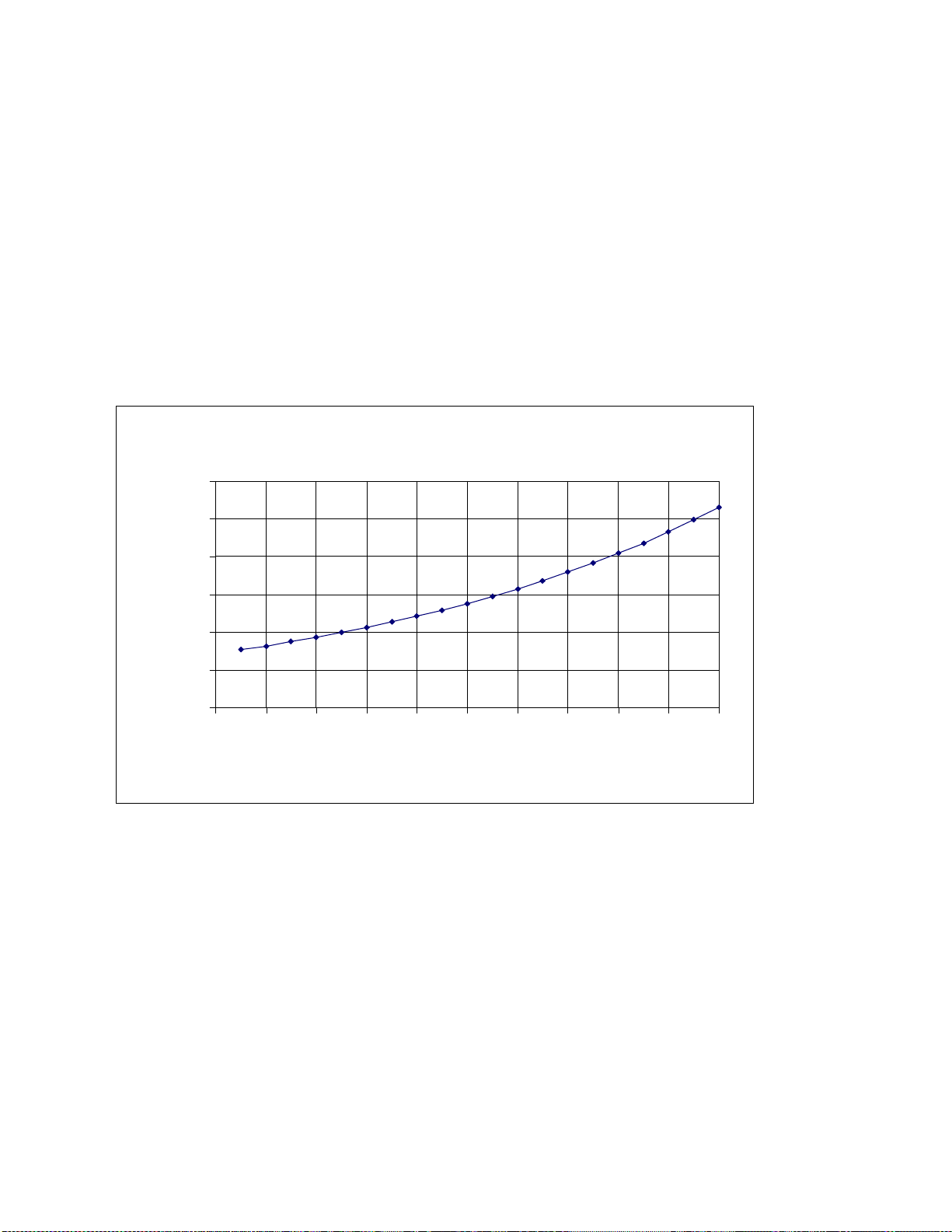
Relative Sensitivity
The relative sensitivity is a way of comparing the expected resolution of the system. The relative
sensitivity is computed such that a system with a relative sensitivity of 1 would have resolution
of 0.005%FR peak-to-peak when measured at a 1kHz bandwidth with the sensors positioned at
the extreme end of the measuring range. The resolution at null is generally better by a factor of
3. A relative sensitivity of 0.5 would effectively double the noise in the system and the
temperature coefficient in the electronics as a percent of the measuring range (i.e. 1 is good, 0.5
is not as good).
This also affects the temperature coefficient of the electronics in the same relative manner. At a
relative sensitivity of 1 the electronics would have a temperature coefficient of approximately
±0.01 to 0.02%FR/
o
C (typically).
Estimated Relative Sensitivity of KD5100
1.20
1.00
0.80
0.60
0.40
Relative Sensitivity
0.20
0.00
0% 10% 20% 30% 40% 50% 60% 70% 80% 90% 100%
Full Range a s % of Coil Diam e ter
The reason that this has an optimum around 35% of the measuring range is because of the
following:
• At large ranges the output change remains constant while the range is increasing. This
sensitivity number would obviously have a limit at ‘0’ as the range increased to infinity.
• At small ranges the output change is diminishing faster than the range is decreasing resulting
in a net loss of sensitivity as a percentage of the measuring range.
34
Page 35

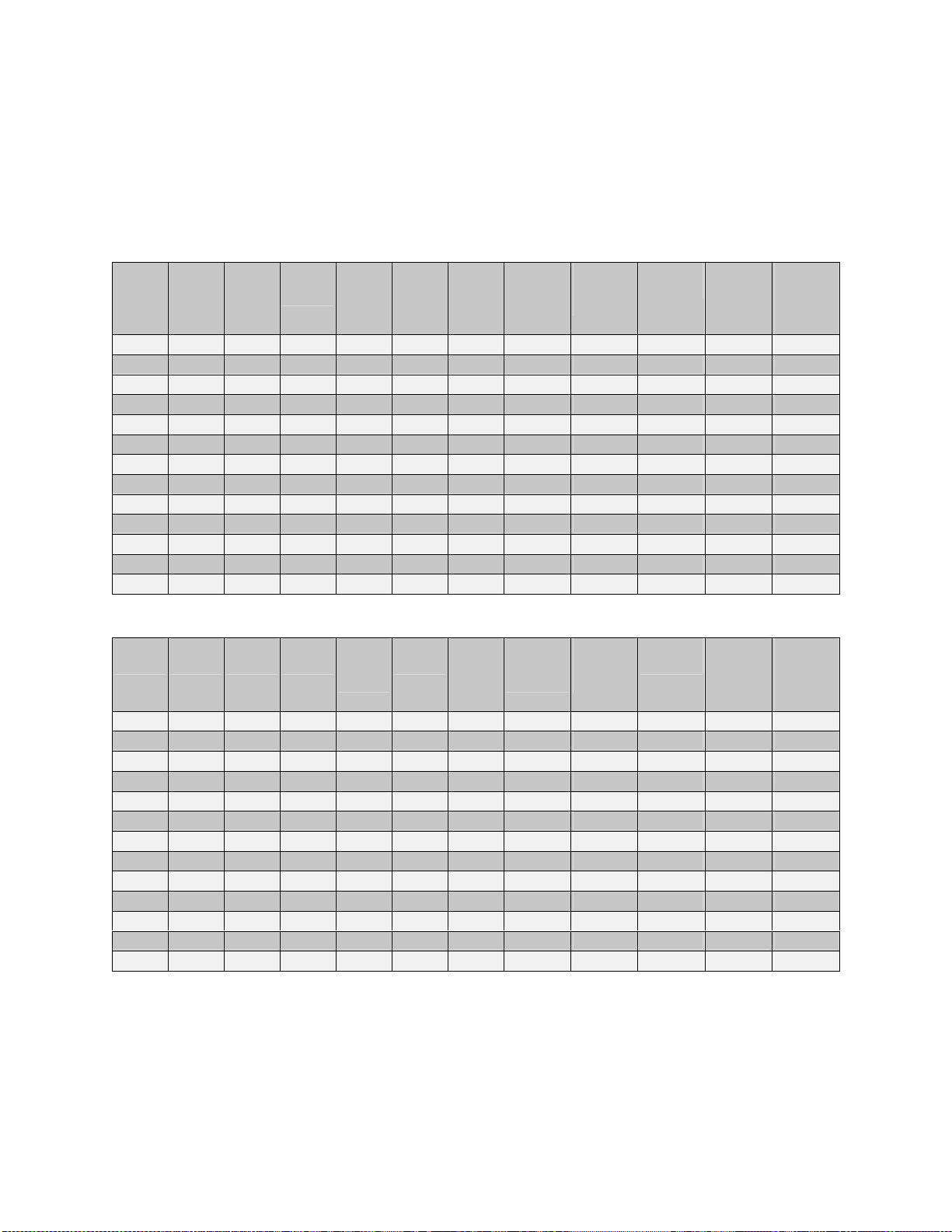
Specific Example: 15N Sensors
The estimates below are for a 15N sensor. The estimates are based on the coil diameter of 143
mils (3.63mm). The two tables contain the same data, just in different units. Note there is an
entry for a 2 mil range (+/-1mil) (~50 micron -- +/-25micron). This entry is based on a
considerable amount of experience with this system and was not calculated.
KD5100-15N Sensor -- English Units
%Coil
14% 5 20 15 10 0.15% 0.030 0.02% 0.004 0.40 0.003 0.0008
21% 5 30 20 15 0.17% 0.052 0.02% 0.006 0.60 0.003 0.0008
28% 10 40 30 20 0.25% 0.100 0.03% 0.010 0.80 0.003 0.0008
35% 10 50 35 25 0.35% 0.175 0.03% 0.013 1.00 0.003 0.0008
49% 10 70 45 35 0.50% 0.350 0.03% 0.021 0.60 0.006 0.0019
56% 10 80 50 40 1.00% 0.800 0.03% 0.024 0.50 0.008 0.0027
63% 10 90 55 45 1.20% 1.080 0.04% 0.032 0.30 0.015 0.0050
70% 10 100 60 50 1.60% 1.600 0.04% 0.040 0.30 0.017 0.0056
77% 10 110 65 55 2.20% 2.420 0.04% 0.044 0.20 0.028 0.0092
84% 10 120 70 60 3.00% 3.600 0.05% 0.060 0.20 0.030 0.0100
91% 10 130 75 65 4.20% 5.460 0.05% 0.065 0.20 0.033 0.0108
KD5100-15N Sensor -- Metric Units
%Coil
Dia.
14% 0.127 0.508 0.381 0.254 0.15% 0.76 0.02% 0.10 0.40 0.064 0.0212
21% 0.127 0.762 0.508 0.381 0.17% 1.33 0.02% 0.15 0.60 0.064 0.0212
28% 0.254 1.016 0.762 0.508 0.25% 2.54 0.03% 0.25 0.80 0.064 0.0212
35% 0.254 1.270 0.889 0.635 0.35% 4.45 0.03% 0.32 1.00 0.064 0.0212
49% 0.254 1.778 1.143 0.889 0.50% 8.89 0.03% 0.53 0.60 0.148 0.0494
56% 0.254 2.032 1.270 1.016 1.00% 20.32 0.03% 0.61 0.50 0.203 0.0677
63% 0.254 2.286 1.397 1.143 1.20% 27.43 0.04% 0.80 0.30 0.381 0.1270
70% 0.254 2.540 1.524 1.270 1.60% 40.64 0.04% 1.02 0.30 0.423 0.1411
77% 0.254 2.794 1.651 1.397 2.20% 61.47 0.04% 1.12 0.20 0.699 0.2328
84% 0.254 3.048 1.778 1.524 3.00% 91.44 0.05% 1.52 0.20 0.762 0.2540
91% 0.254 3.302 1.905 1.651 4.20% 138.68 0.05% 1.65 0.20 0.826 0.2752
Offset,
Dia.
1% 6 2 7 1 0.10% 0.002 0.05% 0.001 0.10 0.001 0.0003
7% 5 10 10 5 0.10% 0.010 0.02% 0.002 0.20 0.003 0.0008
Offset,
mm
1% 0.152 0.051 0.178 0.025 0.10% 0.05 0.05% 0.03 0.10 0.025 0.0085
7% 0.127 0.254 0.254 0.127 0.10% 0.25 0.02% 0.05 0.20 0.064 0.0212
mil
Range
,mil
Range,
mm
Null,
mil
Null,
mm
Range
(+/-)
mil
Range
(+/-)
mm
NL,
%FR
NL,
%FR
NL,mil Sensor
TC,
%FR/oC
NL,µµµµm
Sensor
TC,
%FR/oC
Sensor
TC,
mil/oC
Sensor
TC,
µµµµm/oC
Relative
Sens.
Relative
Sens.
FR Res,
mil p-p
@1kHz
FR Res ,
µµµµm p-p
@1kHz
Null
Res,
mil p-p
@1kHz
Null
Res,
µµµµm p-p
@1kHz
35
Page 36
Specific Example: 20N Sensors
The estimates below are for a 20N sensor. The estimates are based on the coil diameter of 363
mils (9.22mm). The two tables contain the same data, just in different units.
KD5100-20N Sensor -- English Units
%Coil
11% 20 40 40 20 0.15% 0.060 0.02% 0.008 0.35 0.006 0.0019
14% 20 50 45 25 0.15% 0.075 0.02% 0.010 0.40 0.006 0.0021
19% 30 70 65 35 0.20% 0.140 0.02% 0.014 0.45 0.008 0.0026
22% 30 80 70 40 0.20% 0.160 0.02% 0.016 0.60 0.007 0.0022
28% 30 100 80 50 0.25% 0.250 0.03% 0.025 0.65 0.008 0.0026
41% 35 150 110 75 0.50% 0.750 0.03% 0.045 1.00 0.008 0.0025
55% 35 200 135 100 1.00% 2.000 0.03% 0.060 0.60 0.017 0.0056
69% 35 250 160 125 1.50% 3.750 0.04% 0.088 0.30 0.042 0.0139
83% 35 300 185 150 3.00% 9.000 0.05% 0.150 0.20 0.075 0.0250
96% 35 350 210 175 5.50% 19.250 0.06% 0.210 0.15 0.117 0.0389
Offset,
Dia.
3% 10 10 15 5 0.10% 0.010 0.02% 0.002 0.10 0.005 0.0017
6% 10 20 20 10 0.10% 0.020 0.02% 0.004 0.20 0.005 0.0017
8% 10 30 25 15 0.10% 0.030 0.02% 0.006 0.30 0.005 0.0017
mil
Range
,mil
Null,
mil
Range
(+/-)
mil
NL,
%FR
NL,mil Sensor
TC,
%FR/oC
Sensor
TC,
mil/oC
Relative
Sens.
FR Res,
mil p-p
@1kHz
Null
Res,
mil p-p
@1kHz
KD5100-20N Sensor -- Metric Units
%Coil
Offset,
Dia.
3% 0.254 0.254 0.381 0.127 0.10% 0.25 0.02% 0.05 0.10 0.127 0.0423
6% 0.254 0.508 0.508 0.254 0.10% 0.51 0.02% 0.10 0.20 0.127 0.0423
8% 0.254 0.762 0.635 0.381 0.10% 0.76 0.02% 0.15 0.30 0.127 0.0423
11% 0.508 1.016 1.016 0.508 0.15% 1.52 0.02% 0.20 0.35 0.145 0.0484
14% 0.508 1.270 1.143 0.635 0.15% 1.91 0.02% 0.25 0.40 0.159 0.0529
19% 0.762 1.778 1.651 0.889 0.20% 3.56 0.02% 0.36 0.45 0.198 0.0659
22% 0.762 2.032 1.778 1.016 0.20% 4.06 0.02% 0.41 0.60 0.169 0.0564
28% 0.762 2.540 2.032 1.270 0.25% 6.35 0.03% 0.64 0.65 0.195 0.0651
41% 0.889 3.810 2.794 1.905 0.50% 19.05 0.03% 1.14 1.00 0.191 0.0635
55% 0.889 5.080 3.429 2.540 1.00% 50.80 0.03% 1.52 0.60 0.423 0.1411
69% 0.889 6.350 4.064 3.175 1.50% 95.25 0.04% 2.22 0.30 1.058 0.3528
83% 0.889 7.620 4.699 3.810 3.00% 228.60 0.05% 3.81 0.20 1.905 0.6350
96% 0.889 8.890 5.334 4.445 5.50% 488.95 0.06% 5.33 0.15 2.963 0.9878
mm
Range,
mm
Null,
mm
Range
(+/-)
mm
NL,
%FR
NL,µµµµm
Sensor
TC,
%FR/oC
Sensor
TC,
µµµµm/oC
Relative
Sens.
FR Res ,
µµµµm p-p
@1kHz
Null
Res,
µµµµm p-p
@1kHz
36
Page 37

Application Variables and Caveats
There are some application variables that will also affect performance. The effects listed are not
considered in the results of this tech note. These effects must be considered separately.
Sensor Loading: Sensor loading by conductive materials that are incidentally in “view” of the
sensors can affect the results significantly and must be considered on a case-by-case basis. The
discussions in this tech note assume that incidental materials do not load the sensor.
Cosine Error: This is error that occurs when the target movement is from tilting as in a fast
steering mirror assembly and can become significant at larger measuring ranges.
Cross Axis Sensitivity Errors: This error occurs in 2 axis measurements of tip and tilt (common
in fast steering mirrors) and can become significant at larger measuring ranges.
Setup Error: The system can become very sensitive to the null gap position when setup for very
small ranges. Changes in the null gap will affect both the sensitivity and temperature coefficient.
Usually only significant problem on ranges of <±10mils (<±0.25mm).
Target Effects: Eddy current sensors are significantly affected by the target material resistivity
and permeability. Aluminum targets are considered in this tech note. In general the KD5100 is
best used with non-magnetic (relative permeability -- µ
this has on the sensor is dependent on the operating frequency and coil diameter.
Cable Length: The sensors used by Kaman are passive. This means that the cable is an integral
part of the sensor and affects the measurement performance. The data presented assumes a 2
meter cable length. Actual results may vary with different cable lengths. Long cables are
especially bad for performance because they degrade the effective Q of the sensor and increase
the inherent temperature coefficient of the sensor coil. Long cables will also cause problems
with thermal drift and variations in the output caused by cable movement.
Optimization: In the data presented the circuit was optimized for each range. This means that
the component values in the circuit may be different for each specific measuring range. The
system will not get the performance shown simply by changing the range and recalibrating – it
would require factory optimization. Also you could optimize on a specific parameter (say
temperature) and achieve better performance in that category – allowing the other performance
parameters to be worse. The data shown for a specific range is a compromise of all the
performance parameters. At each measurement range listed the linearity, temperature
coefficient, and sensitivity listed are achievable simultaneously.
=1), low resistivity targets. The effect
r
37
Page 38

Method of Computing Performance
These results are based mainly on simulations. First the sensor inductance and resistance was
computed using a modeling program. Then the effect of 2 meters of cable was factored in taking
in consideration the transmission line effects of the cable. After that the resultant inductance and
resistance was put in a model to simulate the circuit bridge network. The performance in each
case was optimized to provide temperature coefficient as close to .02%FR as possible while
adjusting the parameters for optimal linearity and reasonably good output. The resulting data
was then fit to exponential curves to provide a continuous function of non-linearity and
temperature coefficient vs. coil diameter (and the fit was very good). Finally, the results were
then adjusted slightly based on data from actual systems and engineering judgement.
This does mean that you can adjust for better temperature coefficient if you are not concerned
with linearity and resolution. You can also get better resolution if you are willing to have a bad
temperature coefficient. The tradeoffs were made to provide the best overall accuracy. What
good is excellent resolution if the temperature coefficient causes the output to drift out of range?
In general the results will be reasonably accurate from about 10-50% of the coil diameter.
Ranges of less than 10% will have additional errors not accounted for such as thermal expansion
of the sensor body. Ranges less than 10% and greater than 50% will also have errors due to
mismatch in the sensors and electronics.
A Note about Small Ranges
There is a point of diminishing returns when the range gets small relative to the coil diameter.
At a range of about 20% of the coil diameter, the amount of change in the measured variable
starts to get small rapidly. This causes the inherent output of the system to be reduced such that
as you add more gain in the electronics to compensate your effective resolution does not increase
(and in fact your noise as a % of the range starts to increase). Also you start to get significant
errors from sensor body thermal expansion and component matching in the electronics. The
‘break even’ point is at a range of about 5% of the coil diameter. This means that reducing the
range will not help your effective performance and your dynamic range will be reduced. A range
that is too small also makes it more difficult to set up the sensor within its measurement range.
Other Observations
1) Performance degrades rapidly when the range is past 50% of the coil diameter.
2) There is a limit (floor) to the resolution and accuracy when operating over very small ranges
(<5% of the coil diameter).
3) The optimum performance will be when operating with a measuring range of approximately
35% of the coil diameter. This is where the best tradeoff between resolution, non-linearity,
and temperature coefficient will be achieved.
38
Page 39

NONCONTACT POSITION MEASURING SYSTEMS
KD5100
Output Filter Characteristics of the KD5100
Applications utilizing the KD5100 as the displacement feedback in closed loop systems
generally require information about the gain and phase delay vs. frequency. The output filter
largely controls these KD5100 characteristics in most applications.
Output Filter Schematic
The output filter is a standard 2 pole butterworth configuration. It is set for a cutoff frequency (3dB) of approximately 23 kHz.
Figure 1 – Output Filter Schematic
39
Page 40

Analysis Results
The filter was analyzed using Micro-Cap V. The plot and table below show the magnitude (dB)
and phase (degrees) output for the standard configuration in the KD5100. The –3dB point is at
about 23kHz. There is a small gain of 1.59 (about +4dB) in the circuit.
) of approximately 23 kHz.
Figure 1 – Output Filter Schematic
Analysis Results
The filter was analyzed using Micro-Cap V. The plot and table below show the magnitude (dB)
and phase (degrees) output for the standard configuration in the KD5100. The –3dB point is at
about 23kHz. There is a small gain of 1.59 (about +4dB) in the circuit.
40
Page 41

Figure 2 – Analysis Results of Magnitude and Phase Vs. Frequency
Frequency, Hz Magnitude, dB Relative
Magnitude, dB
10 +4.03 dB 0.00 0.00
100 +4.03 dB 0.00 -0.36
1000 +4.03 dB 0.00 -3.50
2000 +4.03 dB 0.00 -7.01
5000 +4.02 dB -0.01 -18.72
10000 +3.74 dB -0.29 -38.8
20000 +2.17 dB -1.86 -78.50
23600 +0.94 dB -3.09 -91.71
Table 1 – Summary of Gain and Phase Characteristics on Output Filter of KD5100
Phase Shift,
degrees
41
 Loading...