Juniper JUNOSE 11.1.X - QUALITY OF SERVICE CONFIGURATION GUIDE 3-21-2010, JUNOSe 11.1.X Configuration Manual

JUNOSe™ Software
for E Series™ Broadband Services Routers

Quality of Service Configuration Guide

Release 11.1.x

Juniper Networks, Inc.

1194 North Mathilda Avenue

Sunnyvale, California 94089

USA

408-745-2000

www.juniper.net

Published: 2010-03-21

Juniper Networks, the Juniper Networks logo, JUNOS, NetScreen, ScreenOS, and Steel-Belted Radius are registered trademarks of Juniper Networks, Inc. in
the United States and other countries. JUNOSe is a trademark of Juniper Networks, Inc. All other trademarks, service marks, registered trademarks, or
registered service marks are the property of their respective owners.

Juniper Networks assumes no responsibility for any inaccuracies in this document. Juniper Networks reserves the right to change, modify, transfer, or
otherwise revise this publication without notice.

Products made or sold by Juniper Networks or components thereof might be covered by one or more of the following patents that are owned by or licensed
to Juniper Networks: U.S. Patent Nos. 5,473,599, 5,905,725, 5,909,440, 6,192,051, 6,333,650, 6,359,479, 6,406,312, 6,429,706, 6,459,579, 6,493,347,
6,538,518, 6,538,899, 6,552,918, 6,567,902, 6,578,186, and 6,590,785.

JUNOSe™ Software for E Series™ Broadband Services Routers Quality of Service Configuration Guide

Release 11.1.x
Copyright © 2010, Juniper Networks, Inc.
All rights reserved. Printed in USA.

Writing: Krupa Chandrashekar, Bruce Gillham, Sarah Lesway-Ball, Brian Wesley Simmons, Poornima Goswami, Chander Aima
Editing: Benjamin Mann
Illustration: Nathaniel Woodward
Cover Design: Edmonds Design

Revision History
April 2010—FRS JUNOSe 11.1.x

The information in this document is current as of the date listed in the revision history.

YEAR 2000 NOTICE

Juniper Networks hardware and software products are Year 2000 compliant. The JUNOS Software has no known time-related limitations through the year

2038. However, the NTP application is known to have some difficulty in the year 2036.

ii ■

END USER LICENSE AGREEMENT

READ THIS END USER LICENSE AGREEMENT (“AGREEMENT”) BEFORE DOWNLOADING, INSTALLING, OR USING THE SOFTWARE. BY DOWNLOADING,
INSTALLING, OR USING THE SOFTWARE OR OTHERWISE EXPRESSING YOUR AGREEMENT TO THE TERMS CONTAINED HEREIN, YOU (AS CUSTOMER
OR IF YOU ARE NOT THE CUSTOMER, AS A REPRESENTATIVE/AGENT AUTHORIZED TO BIND THE CUSTOMER) CONSENT TO BE BOUND BY THIS
AGREEMENT. IF YOU DO NOT OR CANNOT AGREE TO THE TERMS CONTAINED HEREIN, THEN (A) DO NOT DOWNLOAD, INSTALL, OR USE THE SOFTWARE,
AND (B) YOU MAY CONTACT JUNIPER NETWORKS REGARDING LICENSE TERMS.

1. The Parties. The parties to this Agreement are (i) Juniper Networks, Inc. (if the Customer’s principal office is located in the Americas) or Juniper Networks
(Cayman) Limited (if the Customer’s principal office is located outside the Americas) (such applicable entity being referred to herein as “Juniper”), and (ii)
the person or organization that originally purchased from Juniper or an authorized Juniper reseller the applicable license(s) for use of the Software (“Customer”)
(collectively, the “Parties”).

2. The Software. In this Agreement, “Software” means the program modules and features of the Juniper or Juniper-supplied software, for which Customer
has paid the applicable license or support fees to Juniper or an authorized Juniper reseller, or which was embedded by Juniper in equipment which Customer
purchased from Juniper or an authorized Juniper reseller. “Software” also includes updates, upgrades and new releases of such software. “Embedded
Software” means Software which Juniper has embedded in or loaded onto the Juniper equipment and any updates, upgrades, additions or replacements
which are subsequently embedded in or loaded onto the equipment.

3. License Grant. Subject to payment of the applicable fees and the limitations and restrictions set forth herein, Juniper grants to Customer a non-exclusive
and non-transferable license, without right to sublicense, to use the Software, in executable form only, subject to the following use restrictions:

a. Customer shall use Embedded Software solely as embedded in, and for execution on, Juniper equipment originally purchased by Customer from Juniper
or an authorized Juniper reseller.

b. Customer shall use the Software on a single hardware chassis having a single processing unit, or as many chassis or processing units for which Customer
has paid the applicable license fees; provided, however, with respect to the Steel-Belted Radius or Odyssey Access Client software only, Customer shall use
such Software on a single computer containing a single physical random access memory space and containing any number of processors. Use of the
Steel-Belted Radius or IMS AAA software on multiple computers or virtual machines (e.g., Solaris zones) requires multiple licenses, regardless of whether
such computers or virtualizations are physically contained on a single chassis.

c. Product purchase documents, paper or electronic user documentation, and/or the particular licenses purchased by Customer may specify limits to
Customer’s use of the Software. Such limits may restrict use to a maximum number of seats, registered endpoints, concurrent users, sessions, calls,
connections, subscribers, clusters, nodes, realms, devices, links, ports or transactions, or require the purchase of separate licenses to use particular features,
functionalities, services, applications, operations, or capabilities, or provide throughput, performance, configuration, bandwidth, interface, processing,
temporal, or geographical limits. In addition, such limits may restrict the use of the Software to managing certain kinds of networks or require the Software
to be used only in conjunction with other specific Software. Customer’s use of the Software shall be subject to all such limitations and purchase of all applicable
licenses.

d. For any trial copy of the Software, Customer’s right to use the Software expires 30 days after download, installation or use of the Software. Customer
may operate the Software after the 30-day trial period only if Customer pays for a license to do so. Customer may not extend or create an additional trial
period by re-installing the Software after the 30-day trial period.

e. The Global Enterprise Edition of the Steel-Belted Radius software may be used by Customer only to manage access to Customer’s enterprise network.
Specifically, service provider customers are expressly prohibited from using the Global Enterprise Edition of the Steel-Belted Radius software to support any
commercial network access services.

The foregoing license is not transferable or assignable by Customer. No license is granted herein to any user who did not originally purchase the applicable
license(s) for the Software from Juniper or an authorized Juniper reseller.

4. Use Prohibitions. Notwithstanding the foregoing, the license provided herein does not permit the Customer to, and Customer agrees not to and shall
not: (a) modify, unbundle, reverse engineer, or create derivative works based on the Software; (b) make unauthorized copies of the Software (except as
necessary for backup purposes); (c) rent, sell, transfer, or grant any rights in and to any copy of the Software, in any form, to any third party; (d) remove
any proprietary notices, labels, or marks on or in any copy of the Software or any product in which the Software is embedded; (e) distribute any copy of
the Software to any third party, including as may be embedded in Juniper equipment sold in the secondhand market; (f) use any ‘locked’ or key-restricted
feature, function, service, application, operation, or capability without first purchasing the applicable license(s) and obtaining a valid key from Juniper, even
if such feature, function, service, application, operation, or capability is enabled without a key; (g) distribute any key for the Software provided by Juniper
to any third party; (h) use the Software in any manner that extends or is broader than the uses purchased by Customer from Juniper or an authorized Juniper
reseller; (i) use Embedded Software on non-Juniper equipment; (j) use Embedded Software (or make it available for use) on Juniper equipment that the
Customer did not originally purchase from Juniper or an authorized Juniper reseller; (k) disclose the results of testing or benchmarking of the Software to
any third party without the prior written consent of Juniper; or (l) use the Software in any manner other than as expressly provided herein.

5. Audit. Customer shall maintain accurate records as necessary to verify compliance with this Agreement. Upon request by Juniper, Customer shall furnish
such records to Juniper and certify its compliance with this Agreement.

■ iii

6. Confidentiality. The Parties agree that aspects of the Software and associated documentation are the confidential property of Juniper. As such, Customer
shall exercise all reasonable commercial efforts to maintain the Software and associated documentation in confidence, which at a minimum includes
restricting access to the Software to Customer employees and contractors having a need to use the Software for Customer’s internal business purposes.

7. Ownership. Juniper and Juniper’s licensors, respectively, retain ownership of all right, title, and interest (including copyright) in and to the Software,
associated documentation, and all copies of the Software. Nothing in this Agreement constitutes a transfer or conveyance of any right, title, or interest in
the Software or associated documentation, or a sale of the Software, associated documentation, or copies of the Software.

8. Warranty, Limitation of Liability, Disclaimer of Warranty. The warranty applicable to the Software shall be as set forth in the warranty statement that
accompanies the Software (the “Warranty Statement”). Nothing in this Agreement shall give rise to any obligation to support the Software. Support services
may be purchased separately. Any such support shall be governed by a separate, written support services agreement. TO THE MAXIMUM EXTENT PERMITTED
BY LAW, JUNIPER SHALL NOT BE LIABLE FOR ANY LOST PROFITS, LOSS OF DATA, OR COSTS OR PROCUREMENT OF SUBSTITUTE GOODS OR SERVICES,
OR FOR ANY SPECIAL, INDIRECT, OR CONSEQUENTIAL DAMAGES ARISING OUT OF THIS AGREEMENT, THE SOFTWARE, OR ANY JUNIPER OR
JUNIPER-SUPPLIED SOFTWARE. IN NO EVENT SHALL JUNIPER BE LIABLE FOR DAMAGES ARISING FROM UNAUTHORIZED OR IMPROPER USE OF ANY
JUNIPER OR JUNIPER-SUPPLIED SOFTWARE. EXCEPT AS EXPRESSLY PROVIDED IN THE WARRANTY STATEMENT TO THE EXTENT PERMITTED BY LAW,
JUNIPER DISCLAIMS ANY AND ALL WARRANTIES IN AND TO THE SOFTWARE (WHETHER EXPRESS, IMPLIED, STATUTORY, OR OTHERWISE), INCLUDING
ANY IMPLIED WARRANTY OF MERCHANTABILITY, FITNESS FOR A PARTICULAR PURPOSE, OR NONINFRINGEMENT. IN NO EVENT DOES JUNIPER
WARRANT THAT THE SOFTWARE, OR ANY EQUIPMENT OR NETWORK RUNNING THE SOFTWARE, WILL OPERATE WITHOUT ERROR OR INTERRUPTION,
OR WILL BE FREE OF VULNERABILITY TO INTRUSION OR ATTACK. In no event shall Juniper’s or its suppliers’ or licensors’ liability to Customer, whether
in contract, tort (including negligence), breach of warranty, or otherwise, exceed the price paid by Customer for the Software that gave rise to the claim, or
if the Software is embedded in another Juniper product, the price paid by Customer for such other product. Customer acknowledges and agrees that Juniper
has set its prices and entered into this Agreement in reliance upon the disclaimers of warranty and the limitations of liability set forth herein, that the same
reflect an allocation of risk between the Parties (including the risk that a contract remedy may fail of its essential purpose and cause consequential loss),
and that the same form an essential basis of the bargain between the Parties.

9. Termination. Any breach of this Agreement or failure by Customer to pay any applicable fees due shall result in automatic termination of the license
granted herein. Upon such termination, Customer shall destroy or return to Juniper all copies of the Software and related documentation in Customer’s
possession or control.

10. Taxes. All license fees payable under this agreement are exclusive of tax. Customer shall be responsible for paying Taxes arising from the purchase of
the license, or importation or use of the Software. If applicable, valid exemption documentation for each taxing jurisdiction shall be provided to Juniper prior
to invoicing, and Customer shall promptly notify Juniper if their exemption is revoked or modified. All payments made by Customer shall be net of any
applicable withholding tax. Customer will provide reasonable assistance to Juniper in connection with such withholding taxes by promptly: providing Juniper
with valid tax receipts and other required documentation showing Customer’s payment of any withholding taxes; completing appropriate applications that
would reduce the amount of withholding tax to be paid; and notifying and assisting Juniper in any audit or tax proceeding related to transactions hereunder.
Customer shall comply with all applicable tax laws and regulations, and Customer will promptly pay or reimburse Juniper for all costs and damages related
to any liability incurred by Juniper as a result of Customer’s non-compliance or delay with its responsibilities herein. Customer’s obligations under this
Section shall survive termination or expiration of this Agreement.

11. Export. Customer agrees to comply with all applicable export laws and restrictions and regulations of any United States and any applicable foreign
agency or authority, and not to export or re-export the Software or any direct product thereof in violation of any such restrictions, laws or regulations, or
without all necessary approvals. Customer shall be liable for any such violations. The version of the Software supplied to Customer may contain encryption
or other capabilities restricting Customer’s ability to export the Software without an export license.

12. Commercial Computer Software. The Software is “commercial computer software” and is provided with restricted rights. Use, duplication, or disclosure
by the United States government is subject to restrictions set forth in this Agreement and as provided in DFARS 227.7201 through 227.7202-4, FAR 12.212,
FAR 27.405(b)(2), FAR 52.227-19, or FAR 52.227-14(ALT III) as applicable.

13. Interface Information. To the extent required by applicable law, and at Customer's written request, Juniper shall provide Customer with the interface
information needed to achieve interoperability between the Software and another independently created program, on payment of applicable fee, if any.
Customer shall observe strict obligations of confidentiality with respect to such information and shall use such information in compliance with any applicable
terms and conditions upon which Juniper makes such information available.

14. Third Party Software. Any licensor of Juniper whose software is embedded in the Software and any supplier of Juniper whose products or technology
are embedded in (or services are accessed by) the Software shall be a third party beneficiary with respect to this Agreement, and such licensor or vendor
shall have the right to enforce this Agreement in its own name as if it were Juniper. In addition, certain third party software may be provided with the
Software and is subject to the accompanying license(s), if any, of its respective owner(s). To the extent portions of the Software are distributed under and
subject to open source licenses obligating Juniper to make the source code for such portions publicly available (such as the GNU General Public License
(“GPL”) or the GNU Library General Public License (“LGPL”)), Juniper will make such source code portions (including Juniper modifications, as appropriate)
available upon request for a period of up to three years from the date of distribution. Such request can be made in writing to Juniper Networks, Inc., 1194

N. Mathilda Ave., Sunnyvale, CA 94089, ATTN: General Counsel. You may obtain a copy of the GPL at http://www.gnu.org/licenses/gpl.html, and
a copy of the LGPL at http://www.gnu.org/licenses/lgpl.html.

15. Miscellaneous. This Agreement shall be governed by the laws of the State of California without reference to its conflicts of laws principles. The provisions
of the U.N. Convention for the International Sale of Goods shall not apply to this Agreement. For any disputes arising under this Agreement, the Parties
hereby consent to the personal and exclusive jurisdiction of, and venue in, the state and federal courts within Santa Clara County, California. This Agreement
constitutes the entire and sole agreement between Juniper and the Customer with respect to the Software, and supersedes all prior and contemporaneous

iv ■

agreements relating to the Software, whether oral or written (including any inconsistent terms contained in a purchase order), except that the terms of a
separate written agreement executed by an authorized Juniper representative and Customer shall govern to the extent such terms are inconsistent or conflict
with terms contained herein. No modification to this Agreement nor any waiver of any rights hereunder shall be effective unless expressly assented to in
writing by the party to be charged. If any portion of this Agreement is held invalid, the Parties agree that such invalidity shall not affect the validity of the
remainder of this Agreement. This Agreement and associated documentation has been written in the English language, and the Parties agree that the English
version will govern. (For Canada: Les parties aux présentés confirment leur volonté que cette convention de même que tous les documents y compris tout
avis qui s'y rattaché, soient redigés en langue anglaise. (Translation: The parties confirm that this Agreement and all related documentation is and will be
in the English language)).

■ v

vi ■

Abbreviated Table of Contents

About the Documentation xxix

Part 1 QoS on the E Series Router

Chapter 1 Quality of Service Overview 3

Part 2 Classifying, Queuing, and Dropping Traffic

Chapter 2 Defining Service Levels with Traffic Classes and Traffic-Class Groups 13

Chapter 3 Configuring Queue Profiles for Buffer Management 17

Chapter 4 Configuring Dropping Behavior with RED and WRED 25

Chapter 5 Gathering Statistics for Rates and Events in the Queue 37

Part 3 Scheduling and Shaping Traffic

Chapter 6 QoS Scheduler Hierarchy Overview 45

Chapter 7 Configuring Rates and Weights in the Scheduler Hierarchy 51

Chapter 8 Configuring Strict-Priority Scheduling 59

Chapter 9 Shared Shaping Overview 71

Chapter 10 Configuring Simple Shared Shaping of Traffic 79

Chapter 11 Configuring Variables in the Simple Shared Shaping Algorithm 89

Chapter 12 Configuring Compound Shared Shaping of Traffic 99

Chapter 13 Configuring Implicit and Explicit Constituent Selection for Shaping 107

Chapter 14 Monitoring a QoS Scheduler Hierarchy 123

Part 4 Creating a QoS Scheduler Hierarchy on an Interface with

QoS Profiles

Chapter 15 QoS Profile Overview 127

Chapter 16 Configuring and Attaching QoS Profiles to an Interface 131

Chapter 17 Configuring Shadow Nodes for Queue Management 149

Chapter 18 Monitoring a Scheduler Hierarchy on an Interface with QoS Profiles 155

Part 5 Interface Solutions for QoS

Chapter 19 Configuring an Integrated Scheduler to Provide QoS for ATM 159

Chapter 20 Configuring QoS for Gigabit Ethernet Interfaces and VLAN Subinterfaces 177

Chapter 21 Configuring QoS for 802.3ad Link Aggregation Groups 183

Abbreviated Table of Contents ■ vii

JUNOSe 11.1.x Quality of Service Configuration Guide

Chapter 22 Configuring QoS for L2TP Sessions 197

Chapter 23 Configuring Interface Sets for QoS 207

Part 6 Managing Queuing and Scheduling with QoS Parameters

Chapter 24 QoS Parameter Overview 225

Chapter 25 Configuring a QoS Parameter 229

Chapter 26 Configuring Hierarchical QoS Parameters 261

Chapter 27 Configuring IP Multicast Bandwidth Adjustment with QoS Parameters 269

Chapter 28 Configuring the Shaping Mode for Ethernet with QoS Parameters 281

Chapter 29 Configuring Byte Adjustment for Shaping Rates with QoS Parameters 293

Chapter 30 Configuring the Downstream Rate Using QoS Parameters 301

Part 7 Monitoring and Troubleshooting QoS

Chapter 31 Monitoring QoS on E Series Routers 313

Chapter 32 Troubleshooting QoS 357

Part 8 Index

Index 361

viii ■

Table of Contents

About the Documentation xxix

E Series and JUNOSe Documentation and Release Notes ............................xxix

Audience ....................................................................................................xxix

E Series and JUNOSe Text and Syntax Conventions ....................................xxix

Obtaining Documentation ..........................................................................xxxi

Documentation Feedback ...........................................................................xxxi

Requesting Technical Support .....................................................................xxxi

Self-Help Online Tools and Resources .................................................xxxii

Opening a Case with JTAC ...................................................................xxxii

Part 1 QoS on the E Series Router

Chapter 1 Quality of Service Overview 3

QoS on the E Series Router Overview ..............................................................3

QoS Audience ..................................................................................................4

QoS Platform Considerations ..........................................................................4

Interface Specifiers ...................................................................................5

QoS Terms ......................................................................................................5

QoS Features ...................................................................................................7

Configuring QoS on the E Series Router ..........................................................8

QoS References ...............................................................................................9

Part 2 Classifying, Queuing, and Dropping Traffic

Chapter 2 Defining Service Levels with Traffic Classes and Traffic-Class

Groups 13

Traffic Class and Traffic-Class Groups Overview ............................................13

Configuring Traffic Classes That Define Service Levels ..................................14

Configuring Traffic-Class Groups That Define Service Levels ..........................15

Monitoring Traffic Classes and Traffic-Class Groups for Defined Levels of

Best-Effort Forwarding ............................................................................13

Traffic-Class Groups Overview ................................................................14

Service ....................................................................................................16

Table of Contents ■ ix

JUNOSe 11.1.x Quality of Service Configuration Guide

Chapter 3 Configuring Queue Profiles for Buffer Management 17

Queuing and Buffer Management Overview ..................................................17

Static Oversubscription ...........................................................................18

Dynamic Oversubscription .....................................................................18

Color-Based Thresholding .......................................................................18

Memory Requirements for Queue and Buffers ..............................................19

Guidelines for Managing Queue Thresholds ...................................................19

Guidelines for Configuring a Maximum Threshold ..................................19

Guidelines for Configuring a Minimum Threshold ...................................20

Guidelines for Managing Buffers ....................................................................20

Guidelines for Managing Buffer Starvation ..............................................21

Configuring Queue Profiles to Manage Buffers and Thresholds ......................22

Monitoring Queues and Buffers .....................................................................24

Chapter 4 Configuring Dropping Behavior with RED and WRED 25

Dropping Behavior Overview ........................................................................25

RED and WRED Overview .............................................................................26

Configuring RED ............................................................................................27

Example: Configuring Average Queue Length for RED ..................................28

Example: Configuring Dropping Thresholds for RED .....................................29

Example: Configuring Color-Blind RED ..........................................................29

Configuring WRED ........................................................................................31

Example: Configuring Different Treatment of Colored Packets for WRED .....33

Example: Defining Different Drop Behavior for Each Traffic Class for

WRED .....................................................................................................33

Example: Configuring WRED and Dynamic Queue Thresholds .....................34

Monitoring RED and WRED ..........................................................................36

Chapter 5 Gathering Statistics for Rates and Events in the Queue 37

QoS Statistics Overview .................................................................................37

Rate Statistics .........................................................................................38

Event Statistics ........................................................................................38

Bulk Statistics Support for QoS Statistics .................................................38

Configuring Statistic Profiles for QoS .............................................................39

Configuring Rate Statistics .............................................................................39

Configuring Event Statistics ...........................................................................40

Clearing QoS Statistics on the Egress Queue ..................................................41

Clearing QoS Statistics on the Fabric Queue ..................................................42

Monitoring QoS Statistics for Rates and Events .............................................42

x ■ Table of Contents

Table of Contents

Part 3 Scheduling and Shaping Traffic

Chapter 6 QoS Scheduler Hierarchy Overview 45

Scheduler Hierarchy Overview ......................................................................45

Shaping Rates, Assured Rates, and Relative Weights in a Scheduler

Hierarchy .........................................................................................46

Configuring a Scheduler Hierarchy ................................................................47

Configuring a Scheduler Profile for a Scheduler Node or Queue ....................48

Using Expressions for Bandwidth and Burst Values in a Scheduler Profile .....48

Chapter 7 Configuring Rates and Weights in the Scheduler Hierarchy 51

Rate Shaping and Port Shaping Overview .....................................................51

Configuring Rate Shaping for a Scheduler Node or Queue .............................52

Configuring Port Shaping ..............................................................................53

Static and Hierarchical Assured Rate Overview .............................................54

Configuring an Assured Rate for a Scheduler Node or Queue ........................55

Configuring a Static Assured Rate ...........................................................55

Configuring a Hierarchical Assured Rate .................................................56

Changing the Assured Rate to an HRR Weight ........................................56

Configuring the HRR Weight for a Scheduler Node or Queue ........................57

Chapter 8 Configuring Strict-Priority Scheduling 59

Strict-Priority and Relative Strict-Priority Scheduling Overview .....................59

Relative Strict-Priority Scheduling Overview ...........................................60

Comparison of True Strict Priority with Relative Strict Priority

Scheduling ..............................................................................................61

Schedulers and True Strict Priority ..........................................................61

Schedulers and Relative Strict Priority ....................................................62

Relative Strict Priority on ATM Modules ..................................................63

Oversubscribing ATM Ports ..............................................................64

Minimizing Latency on the SAR Scheduler .......................................64

HRR Scheduler Behavior and Strict-Priority Scheduling ...........................64

Zero-Weight Queues .........................................................................64

Setting the Burst Size in a Shaping Rate ...........................................65

Special Shaping Rate for Nonstrict Queues .......................................65

Configuring Strict-Priority Scheduling ............................................................66

Configuring Relative Strict-Priority Scheduling for Aggregate Shaping

Rates .......................................................................................................68

Chapter 9 Shared Shaping Overview 71

Shared Shaping Overview .............................................................................71

Shared Shaper Terms ....................................................................................72

How Shared Shaping Works ..........................................................................72

Active Constituents for Shared Shaping ..................................................73

Table of Contents ■ xi

JUNOSe 11.1.x Quality of Service Configuration Guide

Guidelines for Configuring Simple and Compound Shared Shaping ...............74

Shared Shaping and Individual Shaping ..................................................74

Shared Shaping and Best-Effort Queues and Nodes ................................74

ATM and Shared Shaping ........................................................................75

Sharing Bandwidth with the SAR ......................................................75

Shared Shaping and Low-CDV Mode ................................................75

Logical Interface Traffic Carried in Other Queues ....................................76

Traffic Starvation and Shared Shaping ....................................................76

Oversubscription and Shared Shaping ....................................................77

Burst Size and Shared Shaping ................................................................77

Chapter 10 Configuring Simple Shared Shaping of Traffic 79

Simple Shared Shaping Overview ..................................................................79

Bandwidth Allocation for Simple Shared Shaping ...................................79

Simple Shared Shaping on the Best-Effort Scheduler Node .....................79

Simple Shared Shaping for Triple-Play Networks ....................................80

Configuring Simple Shared Shaping ..............................................................81

Example: Simple Shared Shaping for ATM VCs .............................................83

Example: Simple Shared Shaping for ATM VPs ..............................................85

Example: Simple Shared Shaping for Ethernet ..............................................86

Chapter 11 Configuring Variables in the Simple Shared Shaping Algorithm 89

Simple Shared Shaping Algorithm Overview .................................................89

Simple Shared Shaper Algorithm Calculations .........................................90

Variables of the Simple Shared Shaper Algorithm ..........................................91

Guidelines for Controlling the Simple Shared Shaper Algorithm ....................93

Configuring Simple Shared Shaper Algorithm Variables ................................93

Sample Process for Controlling the Simple Shared Shaper Algorithm ............95

Chapter 12 Configuring Compound Shared Shaping of Traffic 99

Compound Shared Shaping Overview ...........................................................99

Supported Hardware for Compound Shared Shaping ..............................99

Bandwidth Allocation for Compound Shared Shaping ...........................100

Configuring Compound Shared Shaping ......................................................100

Example: Compound Shared Shaping for ATM VCs .....................................102

Example: Compound Shared Shaping for ATM VPs .....................................104

xii ■ Table of Contents

Chapter 13 Configuring Implicit and Explicit Constituent Selection for

Shaping 107

Constituent Selection for Shared Shaping Overview ....................................107

Types of Shared Shaper Constituents ....................................................108

Implicit Constituent Selection Overview ......................................................109

Implicit Bandwidth Allocation for Compound Shared Shaping ..............111

Weighted Compound Shared Shaping Example ..............................113

Configuring Implicit Constituents for Simple or Compound Shared

Shaping .................................................................................................114

Explicit Constituent Selection Overview ......................................................115

Explicit Shared Shaping Example ..........................................................116

Explicit Weighted Compound Shared Shaping Example .......................117

Configuring Explicit Constituents for Simple or Compound Shared

Shaping .................................................................................................120

Table of Contents

Chapter 14 Monitoring a QoS Scheduler Hierarchy 123

Monitoring QoS Scheduling and Shaping .....................................................123

Part 4 Creating a QoS Scheduler Hierarchy on an Interface with

QoS Profiles

Chapter 15 QoS Profile Overview 127

QoS Profile Overview ..................................................................................127

Managing System Resources for Nodes and Queues ....................................127

Scaling Subscribers on the TFA ASIC with QoS ............................................128

Chapter 16 Configuring and Attaching QoS Profiles to an Interface 131

Supported Interface Types for QoS Profiles .................................................131

Configuring a QoS Profile ............................................................................132

Attaching a QoS Profile to an Interface ........................................................134

Attaching a QoS Profile to a Base Interface ...........................................134

Attaching a QoS Profile to an ATM VP ...................................................134

Attaching a QoS Profile to an S-VLAN ...................................................135

Attaching a QoS Profile to a Port Type ..................................................135

Munged QoS Profile Overview .....................................................................136

Sample Munged QoS Profile Process .....................................................137

Example: Port-Type QoS Profile Attachment ...............................................139

Example: QoS Profile Attachment to Port ....................................................141

Example: Diffserv Configuration with Multiple Traffic-Class Groups ............143

Table of Contents ■ xiii

JUNOSe 11.1.x Quality of Service Configuration Guide

Chapter 17 Configuring Shadow Nodes for Queue Management 149

Shadow Node Overview ..............................................................................149

Shadow Nodes and Scheduler Behavior .......................................................150

Managing System Resources for Shadow Nodes ..........................................151

Configuring Shadow Nodes .........................................................................152

Example: Shadow Nodes over VLAN and IP Queues ....................................153

Example: Shadow Nodes on the Same Traffic-Class Group ..........................154

Example: Shadow Nodes on Different Traffic-Class Groups .........................154

Chapter 18 Monitoring a Scheduler Hierarchy on an Interface with QoS

Profiles 155

Monitoring a Scheduler Hierarchy on an Interface with QoS Profiles ...........155

Part 5 Interface Solutions for QoS

Chapter 19 Configuring an Integrated Scheduler to Provide QoS for ATM 159

ATM Integrated Scheduler Overview ...........................................................159

Backpressure and the Integrated Scheduler ..........................................160

VP Shaping ...........................................................................................161

Integrating the HRR Scheduler and SAR Scheduler ......................................161

Per-Packet Queuing on the SAR Scheduler Overview ..................................163

Operational QoS Shaping Mode for ATM Interfaces Overview ..............164

ERX7xx Models, ERX14xx Models, and the ERX310 Router ...........164

E120 Router and E320 Router ........................................................165

Guidelines for Configuring QoS over ATM ...................................................166

Configuring Default Integrated Mode for ATM Interface ..............................168

Configuring Low-Latency Mode for Per-Port Queuing on ATM Interfaces ....169

Configuring Low-CDV Mode for Per-Port Queuing on ATM Interfaces ..........171

Configuring the QoS Shaping Mode for ATM Interfaces ...............................174

Disabling Per-Port Queuing on ATM Interfaces ............................................175

Monitoring QoS Configurations for ATM ......................................................175

Chapter 20 Configuring QoS for Gigabit Ethernet Interfaces and VLAN

Subinterfaces 177

Providing QoS for Ethernet Overview ..........................................................177

QoS Shaping Mode for Ethernet Interfaces Overview ..................................178

Configuring the QoS Shaping Mode for Ethernet Interfaces .........................179

Creating a QoS Interface Hierarchy for Bulk-Configured VLAN Subinterfaces

Monitoring QoS Configurations for Ethernet ................................................182

xiv ■ Table of Contents

with RADIUS .........................................................................................180

Table of Contents

Chapter 21 Configuring QoS for 802.3ad Link Aggregation Groups 183

QoS for 802.3ad Link Aggregation Interfaces Overview ..............................183

Types of Load Balancing .......................................................................183

Munged QoS Profiles and Load Balancing .............................................184

802.3ad Link Aggregation and QoS Parameters ....................................184

QoS and Ethernet Link Redundancy .....................................................185

Active Link Failure and QoS ...........................................................185

Administratively Disabling a Link and QoS .....................................185

Adding a New Link to the LAG and QoS .........................................185

Hashed Load Balancing for 802.3ad Link Aggregation Groups Overview .....186

Sample Scheduler Hierarchy for Hashed Load Balancing ......................186

Subscriber Load Balancing for 802.3ad Link Aggregation Groups

Overview ..............................................................................................186

S-VLANs and Subscriber Load Balancing ...............................................187

PPPoE over VLANs and Subscriber Load Balancing ...............................187

PPPoE over Ethernet (No VLANs) and Subscriber Load Balancing .........187

MPLS over LAG and Subscriber Load Balancing ....................................187

Sample Scheduler Hierarchy for Subscriber Load Balancing ..................188

Subscriber Allocation in 802.3ad Link Aggregation Groups ...................189

Guidelines for Configuring QoS over 802.3ad Link Aggregation Groups ......190

Configuring the Scheduler Hierarchy for Hashed Load Balancing in 802.3ad

Link Aggregation Groups .......................................................................191

Enabling Default Subscriber Load Balancing for 802.3ad Link Aggregation

Groups ..................................................................................................191

Configuring the Scheduler Hierarchy for Subscriber Load Balancing in 802.3ad

Link Aggregation Groups .......................................................................192

Configuring Load Rebalancing for 802.3ad Link Aggregation Groups ..........193

Configuring Load–Rebalancing Parameters ...........................................193

Configuring the System to Dynamically Rebalance the LAG ..................195

Monitoring QoS Configurations for 802.3ad Link Aggregation Groups .........195

Chapter 22 Configuring QoS for L2TP Sessions 197

Providing QoS for L2TP Overview ...............................................................197

Sample Scheduler Hierarchies for L2TP .......................................................197

Configuring QoS for an L2TP Session ..........................................................199

Configuring QoS for Tunnel-Server Ports for L2TP LNS Sessions .................202

QoS and L2TP TX Speed AVP 24 Overview .................................................203

Monitoring QoS Configurations for L2TP .....................................................204

Configuring QoS for an L2TP LNS Session .............................................200

Configuring QoS for an L2TP LAC Session ............................................201

Logical Interfaces and Shared-Shaping Rates ........................................203

Shaping Mode .......................................................................................204

Table of Contents ■ xv

JUNOSe 11.1.x Quality of Service Configuration Guide

Chapter 23 Configuring Interface Sets for QoS 207

Interface Sets for QoS Overview ..................................................................207

Interface Set Terms ...............................................................................207

Architecture of Interface Sets for QoS .........................................................208

Interface Set Parents and Types ............................................................209

Sample Interface Columns and Scheduler Hierarchies ..........................209

Scheduling and Shaping Interface Sets ..................................................210

Configuring Interface Sets for Scheduling and Queuing ...............................211

Configuring Interface Supersets for QoS ......................................................212

Configuring an Interface Superset .........................................................212

Restricting an Interface Superset to an S-VLAN ID or an ATM VP ..........212

Configuring Interface Sets for QoS ..............................................................213

Configuring an Interface Set .................................................................213

Deleting an Interface Set from an Interface Superset ............................213

Adding Member Interfaces to an Interface Set .............................................214

Adding Interfaces to an Interface Set with the CLI ................................214

Adding Interfaces to an Interface Set with RADIUS ...............................215

Changing and Deleting Interface Members in an Interface Set ..............215

Changing Interface Members with Upper-Layer Protocols in an Interface

Set ..................................................................................................215

Creating a QoS Parameter on an Interface Superset or Interface Set ...........216

Configuring a QoS Parameter Definition for an Interface Superset or an

Interface Set ...................................................................................216

Creating a QoS Parameter Instance for an Interface Superset ...............217

Creating a QoS Parameter Instance for an Interface Set ........................217

Attaching a QoS Profile to an Interface Superset or an Interface Set ............218

Configuring a QoS Profile for an Interface Superset or an Interface

Set ..................................................................................................218

Attaching a QoS Profile to an Interface Superset ...................................218

Attaching a QoS Profile to an Interface Set ...........................................219

Deleting an Interface Superset or an Interface Set .......................................219

Deleting an Interface Superset ..............................................................219

Deleting an Interface Set .......................................................................220

Example: Configuring Interface Sets for 802.3ad Link Aggregation

Groups ..................................................................................................220

Part 6 Managing Queuing and Scheduling with QoS Parameters

Chapter 24 QoS Parameter Overview 225

QoS Parameter Overview ............................................................................225

QoS Parameter Audience ............................................................................225

QoS Parameter Terms .................................................................................226

xvi ■ Table of Contents

Table of Contents

Relationship Among QoS Parameters, Scheduler Profiles, and QoS

Profiles .................................................................................................227

QoS Administrator Tasks ......................................................................227

QoS Client Tasks ...................................................................................228

Chapter 25 Configuring a QoS Parameter 229

Parameter Definition Attributes for QoS Administrators Overview ..............229

Naming Guidelines for QoS Parameters ................................................230

Interface Types and QoS Parameters ....................................................231

Controlled-Interface Types .............................................................231

Instance-Interface Types ................................................................232

Subscriber-Interface Types .............................................................233

Range of QoS Parameters .....................................................................234

Applications and QoS Parameters .........................................................235

Scheduler Profiles and Parameter Expressions for QoS Administrators .......235

Referencing a Parameter Definition in a Scheduler Profile ....................235

Removing or Modifying a Scheduler Profile ....................................236

Using Expressions for QoS Parameters .................................................236

Operators and Precedence .............................................................236

Specifying a Range in Expressions .................................................237

Configuring a Basic Parameter Definition for QoS Administrators ...............238

Parameter Instances for QoS Clients Overview ...........................................240

Global QoS Parameter Instance Overview .............................................240

QoS Parameters for Interfaces Overview ..............................................241

Creating Parameter Instances ......................................................................242

Creating a Global Parameter Instance ...................................................242

Creating a Parameter Instance for an Interface .....................................242

Creating a Parameter Instance for an ATM VP ......................................242

Creating a Parameter Instance for an S-VLAN .......................................243

Example: QoS Parameter Configuration for Controlling Subscriber

Bandwidth ............................................................................................243

Procedure for QoS Administrators ........................................................245

Procedure for QoS Clients .....................................................................250

Monitoring the Subscriber Configuration ..............................................252

Complete Configuration Example .........................................................256

QoS Administrator Configuration ...................................................256

QoS Client Configuration ................................................................258

Chapter 26 Configuring Hierarchical QoS Parameters 261

Hierarchical QoS Parameters Overview .......................................................261

Guidelines for Configuring Hierarchical Parameters ....................................261

Configuring a Parameter Definition to Calculate Hierarchical Instances ......262

Example: QoS Parameter Configuration for Hierarchical Parameters ..........263

Procedure for QoS Administrators ........................................................264

Procedure for QoS Clients .....................................................................265

Monitoring Hierarchical QoS Parameters ..............................................266

Table of Contents ■ xvii

JUNOSe 11.1.x Quality of Service Configuration Guide

Complete Configuration Example .........................................................267

QoS Administrator Configuration ...................................................267

QoS Client Configuration ................................................................267

Chapter 27 Configuring IP Multicast Bandwidth Adjustment with QoS

Parameters 269

IP Multicast Bandwidth Adjustment for QoS Overview ................................269

Guidelines for Configuring IP Multicast Adjustment for QoS ........................271

Configuring a Parameter Definition for IP Multicast Bandwidth

Adjustment ...........................................................................................271

Example: QoS Parameter Configuration for IP Multicast Bandwidth

Adjustment ...........................................................................................273

Monitoring the Configuration ................................................................276

Complete Configuration Example .........................................................279

Chapter 28 Configuring the Shaping Mode for Ethernet with QoS Parameters 281

Cell Shaping Mode Using QoS Parameters Overview ...................................281

Overriding the QoS Shaping Mode ........................................................281

Module Types and Capabilities for QoS Cell Mode Application ..............282

Cell Tax Adjustment Using QoS Cell Mode ............................................282

Relationship with QoS Downstream Rate Application ...........................283

Guidelines for Configuring the Cell Shaping Mode with QoS Parameters .....283

Configuring a Parameter Definition to Shape Ethernet Traffic Using Cell

Mode ....................................................................................................284

Example: QoS Parameter Configuration for QoS Cell Mode and Byte

Adjustment for Cell Shaping ..................................................................286

Complete Configuration Example .........................................................290

Chapter 29 Configuring Byte Adjustment for Shaping Rates with QoS

Parameters 293

Byte Adjustment for ADSL and VDSL Traffic Overview ................................293

Byte Adjustment for Cell Shaping of ADSL Traffic Overview .................293

Calculation and Example of Byte Adjustment for Cell Shaping .......294

Byte Adjustment for Frame Shaping of VDSL Traffic Overview .............295

System Calculation for Byte Adjustment of ADSL and VDSL Traffic ......295

Guidelines for Configuring Byte Adjustment of Cell and Frame Shaping Rates

Using QoS Parameters ..........................................................................296

Configuring a Parameter Definition to Adjust Cell Shaping Rates for ADSL

Traffic ...................................................................................................297

Configuring a Parameter Definition to Adjust Frame Shaping Rates for VDSL

Traffic ...................................................................................................299

xviii ■ Table of Contents

Table of Contents

Chapter 30 Configuring the Downstream Rate Using QoS Parameters 301

QoS Downstream Rate Application Overview ..............................................301

Downstream Rate and the Shaping Mode .............................................301

QoS Adaptive Mode and Downstream Rate ..........................................302

Obtaining Downstream Rates from a DSL Forum VSA ..........................302

Guidelines for Configuring QoS Downstream Rate ......................................303

Configuring a Parameter Definition for QoS Downstream Rate ...................303

Example: QoS Parameter Configuration for QoS Downstream Rate ............305

Complete Configuration Example .........................................................309

Part 7 Monitoring and Troubleshooting QoS

Chapter 31 Monitoring QoS on E Series Routers 313

Monitoring Service Levels with Traffic Classes .............................................314

Monitoring Service Levels with Traffic-Class Groups ....................................315

Monitoring Queue Thresholds .....................................................................316

Monitoring Queue Profiles ...........................................................................319

Monitoring Drop Profiles for RED and WRED ..............................................320

Monitoring the QoS Scheduler Hierarchy .....................................................322

Monitoring the Configuration of Scheduler Profiles .....................................327

Monitoring Shared Shapers .........................................................................329

Monitoring Shared Shaper Algorithm Variables ...........................................330

Monitoring Forwarding and Drop Events on the Egress Queue ...................331

Monitoring Forwarding and Drop Rates on the Egress Queue .....................333

Monitoring Queue Statistics for the Fabric ...................................................337

Monitoring the Configuration of Statistics Profiles .......................................338

Monitoring the QoS Profiles Attached to an Interface ..................................339

Monitoring the Configuration of QoS Port-Type Profiles ..............................340

Monitoring the Configuration of QoS Profiles ..............................................341

Monitoring the QoS Configuration of ATM Interfaces ..................................343

Monitoring the QoS Configuration of IP Interfaces ......................................345

Monitoring the QoS Configuration of Fast Ethernet, Gigabit Ethernet, and

10-Gigabit Ethernet Interfaces ...............................................................347

Monitoring the QoS Configuration of IEEE 802.3ad Link Aggregation Group

Bundles .................................................................................................349

Monitoring the Configuration of QoS Interface Sets .....................................350

Monitoring the Configuration of QoS Interface Supersets ............................351

Monitoring the AAA Downstream Rate for QoS ...........................................352

Monitoring QoS Parameter Instances ..........................................................352

Monitoring QoS Parameter Definitions ........................................................355

Table of Contents ■ xix

JUNOSe 11.1.x Quality of Service Configuration Guide

Chapter 32 Troubleshooting QoS 357

Troubleshooting Memory and Processor Use for Egress Queue Rate Statistics

and Events ............................................................................................357

Part 8 Index

Index ...........................................................................................................361

xx ■ Table of Contents

List of Figures

Part 1 QoS on the E Series Router

Chapter 1 Quality of Service Overview 3

Figure 1: Traffic Flow Through an E Series Router ...........................................4

Part 2 Classifying, Queuing, and Dropping Traffic

Chapter 4 Configuring Dropping Behavior with RED and WRED 25

Figure 2: Packets Dropped as Queue Length Increases ..................................27

Figure 3: Color-Blind RED Drop Profile with Colorless Queue Profile .............30

Figure 4: Color-Blind RED Drop Profile with Color-Sensitive Queue

Profile .....................................................................................................30

Figure 5: Different Treatment of Colored Packets ..........................................33

Figure 6: Defining Different Drop Behavior for Each Queue ..........................34

Figure 7: WRED and Dynamic Queue Thresholding ......................................36

Part 3 Scheduling and Shaping Traffic

Chapter 6 QoS Scheduler Hierarchy Overview 45

Figure 8: QoS Scheduler Hierarchy ................................................................46

Chapter 7 Configuring Rates and Weights in the Scheduler Hierarchy 51

Figure 9: Port Shaping on an Ethernet Module ..............................................52

Figure 10: Hierarchical Assured Rate .............................................................55

Chapter 8 Configuring Strict-Priority Scheduling 59

Figure 11: Sample Strict-Priority Scheduling Hierarchy ..................................60

Figure 12: True Strict-Priority Configuration ..................................................62

Figure 13: Relative Strict-Priority Configuration .............................................63

Figure 14: Tuning Latency on Strict-Priority Queues ......................................66

Figure 15: Sample Strict-Priority Scheduling Hierarchy ..................................67

Figure 16: Sample Relative Strict-Priority Scheduler Hierarchy ......................69

Chapter 9 Shared Shaping Overview 71

Figure 17: Implicit Constituent Selection for Compound Shared Shaper: Mixed

Interface Types .......................................................................................76

Chapter 10 Configuring Simple Shared Shaping of Traffic 79

Figure 18: Simple Shared Shaping over ATM .................................................80

Figure 19: Simple Shared Shaping over Ethernet ...........................................81

Figure 20: VP Shared Shaping .......................................................................85

Figure 21: Hierarchical Simple Shared Shaping over Ethernet .......................86

Chapter 11 Configuring Variables in the Simple Shared Shaping Algorithm 89

Figure 22: Simple Shared Shaper Behavior Without Algorithm Controls ........89

List of Figures ■ xxi

JUNOSe 11.1.x Quality of Service Configuration Guide

Figure 23: Less Conservative Simple Shared Shaper Behavior .......................90

Figure 24: More Liberal Simple Shared Shaper Behavior ...............................90

Figure 25: Dynamic Rate When Video Flow Starts ........................................96

Figure 26: Dynamic Rate When Video Flow Stops .........................................97

Chapter 12 Configuring Compound Shared Shaping of Traffic 99

Figure 27: VC Compound Shared Shaping Example ....................................102

Figure 28: VP Compound Shared Shaping Example ....................................105

Chapter 13 Configuring Implicit and Explicit Constituent Selection for Shaping 107

Figure 29: Implicit Constituent Selection for Compound Shared Shaper at

Best-Effort Node ....................................................................................110

Figure 30: Implicit Constituent Selection for Compound Shared Shaper at

Best-Effort Queue ..................................................................................111

Figure 31: Weighted Shared Shaping ...........................................................113

Figure 32: Implicit Constituent Selection for Compound Shared Shaper: Mixed

Interface Types .....................................................................................114

Figure 33: Explicit Constituent Selection .....................................................117

Figure 34: Case 1: Explicit Constituent Selection with Weighted

Constituents ..........................................................................................118

Figure 35: Case 2: Explicit Constituent Selection with Weighted

Constituents ..........................................................................................119

Part 4 Creating a QoS Scheduler Hierarchy on an Interface with

QoS Profiles

Chapter 16 Configuring and Attaching QoS Profiles to an Interface 131

Figure 36: Munged Profile Example .............................................................138

Figure 37: Attaching QoS Profiles to ATM Subinterfaces ..............................139

Figure 38: Attaching QoS Profile to ATM Interface and Subinterface ...........142

Figure 39: Diffserv Configuration with Multiple Traffic-Class Groups ...........146

Figure 40: Diffserv Configuration Without Traffic-Class Groups ...................147

Chapter 17 Configuring Shadow Nodes for Queue Management 149

Figure 41: Phantom Nodes ..........................................................................150

Figure 42: Shadow Nodes ............................................................................151

Part 5 Interface Solutions for QoS

Chapter 19 Configuring an Integrated Scheduler to Provide QoS for ATM 159

Figure 43: Integrated ATM Scheduler ..........................................................161

Figure 44: Default Integrated Mode .............................................................168

Figure 45: Low-Latency Mode ......................................................................170

Figure 46: Low-CDV Mode (per-VP CDVT) ...................................................172

Figure 47: Low-CDV Mode (per-VC CDVT) ...................................................172

Chapter 21 Configuring QoS for 802.3ad Link Aggregation Groups 183

Figure 48: 802.3ad Link Aggregation Scheduler Hierarchy ..........................186

Figure 49: Subscriber LoadBalanced Scheduler Hierarchy for Port 0 ...........188

Figure 50: Subscriber LoadBalanced Scheduler Hierarchy for Port 1 ...........189

Figure 51: Subscriber Allocation and Load Balancing ..................................189

Chapter 22 Configuring QoS for L2TP Sessions 197

xxii ■ List of Figures

List of Figures

Figure 52: LNS (Non-MLPPP) Scheduler Hierarchy .......................................198

Figure 53: LNS (MLPPP) QoS Scheduler Hierarchy .......................................198

Figure 54: LAC over Ethernet (Without VLANs) Scheduler Hierarchy ...........198

Figure 55: LAC over Ethernet (With LANs) Scheduler Hierarchy ..................199

Figure 56: LAC over ATM ............................................................................199

Chapter 23 Configuring Interface Sets for QoS 207

Figure 57: VLAN Interface Column with Interface Sets ................................210

Figure 58: Scheduler Hierarchy with Nodes at Interface Set and Superset ....210

Part 6 Managing Queuing and Scheduling with QoS Parameters

Chapter 24 QoS Parameter Overview 225

Figure 59: Relationship of Parameter Definitions, Scheduler Profiles, and

QoS Profiles ..........................................................................................227

Chapter 25 Configuring a QoS Parameter 229

Figure 60: Physical Network Topology ........................................................244

Figure 61: QoS Scheduler Hierarchy ............................................................244

Chapter 26 Configuring Hierarchical QoS Parameters 261

Figure 62: Hierarchical Parameters Scheduler Hierarchy .............................264

Chapter 27 Configuring IP Multicast Bandwidth Adjustment with QoS Parameters 269

Figure 63: Scheduler Hierarchy with QoS Adjustment for IP Multicast .........274

Chapter 28 Configuring the Shaping Mode for Ethernet with QoS Parameters 281

Figure 64: Byte Adjustment for VC1 and VC2 ..............................................286

Chapter 29 Configuring Byte Adjustment for Shaping Rates with QoS Parameters 293

Figure 65: Byte Adjustment Calculation for Ethernet and ATM

Encapsulations ......................................................................................294

List of Figures ■ xxiii

JUNOSe 11.1.x Quality of Service Configuration Guide

xxiv ■ List of Figures

List of Tables

About the Documentation xxix

Table 1: Notice Icons ...................................................................................xxx

Table 2: Text and Syntax Conventions ........................................................xxx

Part 1 QoS on the E Series Router

Chapter 1 Quality of Service Overview 3

Table 3: QoS Terminology ...............................................................................5

Table 4: QoS Features .....................................................................................7

Part 2 Classifying, Queuing, and Dropping Traffic

Chapter 3 Configuring Queue Profiles for Buffer Management 17

Table 5: Egress Memory and Region Size on ASIC Line Modules ...................19

Part 3 Scheduling and Shaping Traffic

Chapter 9 Shared Shaping Overview 71

Table 6: Shared Shaper Terminology Used in This Chapter ...........................72

Table 7: Comparison of Simple and Compound Shared Shaping ...................73

Chapter 11 Configuring Variables in the Simple Shared Shaping Algorithm 89

Table 8: Guidelines for Configuring Simple Shared Shaper Algorithm

Variables .................................................................................................93

Table 9: Rising Edge Sample When Video Flow Starts ...................................95

Table 10: Data When Video Flow Stops .........................................................96

Chapter 13 Configuring Implicit and Explicit Constituent Selection for Shaping 107

Table 11: Comparison of Implicit and Explicit Shared Shaping ....................108

Table 12: Bandwidth Allocation for Case 1 Explicit Constituents .................118

Table 13: Bandwidth Allocation for Case 2 Explicit Constituents .................119

Part 4 Creating a QoS Scheduler Hierarchy on an Interface with

QoS Profiles

Chapter 16 Configuring and Attaching QoS Profiles to an Interface 131

Table 14: Interface Types and Supported Commands .................................131

Chapter 17 Configuring Shadow Nodes for Queue Management 149

Table 15: Shadow Node Consumption of Node and Queue Resources .........152

List of Tables ■ xxv

JUNOSe 11.1.x Quality of Service Configuration Guide

Part 5 Interface Solutions for QoS

Chapter 19 Configuring an Integrated Scheduler to Provide QoS for ATM 159

Table 16: qos-mode-port Commands ..........................................................162

Table 17: Operational Shaping Modes for ERX7xx Models, ERX14xx Models,

and the ERX310 Router ........................................................................165

Table 18: Operational Shaping Modes for the E120 Router and E320

Router ...................................................................................................166

Chapter 20 Configuring QoS for Gigabit Ethernet Interfaces and VLAN Subinterfaces 177

Table 19: Operational Shaping Modes .........................................................178

Chapter 21 Configuring QoS for 802.3ad Link Aggregation Groups 183

Table 20: Load Balancing Algorithm Parameters .........................................193

Chapter 23 Configuring Interface Sets for QoS 207

Table 21: Interface Set Terms ......................................................................208

Part 6 Managing Queuing and Scheduling with QoS Parameters

Chapter 24 QoS Parameter Overview 225

Table 22: QoS Parameter Terminology Used in This Chapter ......................226

Chapter 25 Configuring a QoS Parameter 229

Table 23: Attributes in Parameter Definitions ..............................................229

Table 24: Sample Parameter Names ...........................................................230

Table 25: Valid and Invalid Parameter Names .............................................231

Table 26: Operators for Parameter Expressions ..........................................237

Chapter 28 Configuring the Shaping Mode for Ethernet with QoS Parameters 281

Table 27: Supported Interfaces for qos-shaping-mode and qos-cell-mode

Commands ...........................................................................................282

Table 28: Byte Adjustment for Subscribers VC1 and VC2 ............................286

Chapter 29 Configuring Byte Adjustment for Shaping Rates with QoS Parameters 293

Table 29: Header Lengths for Ethernet Encapsulation .................................294

Table 30: Header Lengths for ATM Encapsulation .......................................295

Table 31: Byte Adjustment Values for Frame and Cell Shaping Modes ........296

Chapter 30 Configuring the Downstream Rate Using QoS Parameters 301

Table 32: Access Loop Types and Resultant Shaping Mode .........................302

Table 33: Shaping Rate and Shaping Mode ..................................................306

Part 7 Monitoring and Troubleshooting QoS

Chapter 31 Monitoring QoS on E Series Routers 313

Table 34: show traffic-class Output Fields ...................................................314

Table 35: show traffic-class-group Output Fields .........................................315

Table 36: show qos queue-thresholds Output Fields ....................................319

Table 37: show queue-profile Output Fields .................................................320

Table 38: show drop-profile Output Fields ...................................................321

Table 39: show qos scheduler-hierarchy Output Fields ................................327

Table 40: show scheduler-profile Output Fields ...........................................328

Table 41: show qos shared-shaper Output Fields .........................................330

Table 42: show qos shared-shaper-control Output Fields .............................331

xxvi ■ List of Tables

List of Tables

Table 43: show egress-queue events Output Fields ......................................332

Table 44: show egress-queue rates Output Fields ........................................335

Table 45: show fabric-queue Output Fields ..................................................337

Table 46: show statistics-profile Output Fields .............................................338

Table 47: show qos interface-hierarchy Output Fields .................................339

Table 48: show qos-profile Output Fields .....................................................342

Table 49: show interfaces atm Output Fields ...............................................344

Table 50: show ip interface Output Fields ...................................................346

Table 51: show interfaces Output Fields ......................................................348

Table 52: show interfaces lag members Output Fields .................................349

Table 53: show qos-interface-set Output Fields ...........................................350

Table 54: show qos-interface-superset Output Fields ...................................351

Table 55: show aaa qos downstream-rate Output Fields ..............................352

Table 56: show qos-parameter Output Fields ..............................................354

Table 57: show qos-parameter-define Output Fields ....................................355

List of Tables ■ xxvii

JUNOSe 11.1.x Quality of Service Configuration Guide

xxviii ■ List of Tables

About the Documentation

■ E Series and JUNOSe Documentation and Release Notes on page xxix

■ Audience on page xxix

■ E Series and JUNOSe Text and Syntax Conventions on page xxix

■ Obtaining Documentation on page xxxi

■ Documentation Feedback on page xxxi

■ Requesting Technical Support on page xxxi

E Series and JUNOSe Documentation and Release Notes

For a list of related JUNOSe documentation, see

http://www.juniper.net/techpubs/software/index.html .

If the information in the latest release notes differs from the information in the
documentation, follow the JUNOSe Release Notes.

To obtain the most current version of all Juniper Networks® technical documentation,
see the product documentation page on the Juniper Networks website at

http://www.juniper.net/techpubs/.

Audience

This guide is intended for experienced system and network specialists working with
Juniper Networks E Series Broadband Services Routers in an Internet access
environment.

E Series and JUNOSe Text and Syntax Conventions

Table 1 on page xxx defines notice icons used in this documentation.

E Series and JUNOSe Documentation and Release Notes ■ xxix

JUNOSe 11.1.x Quality of Service Configuration Guide

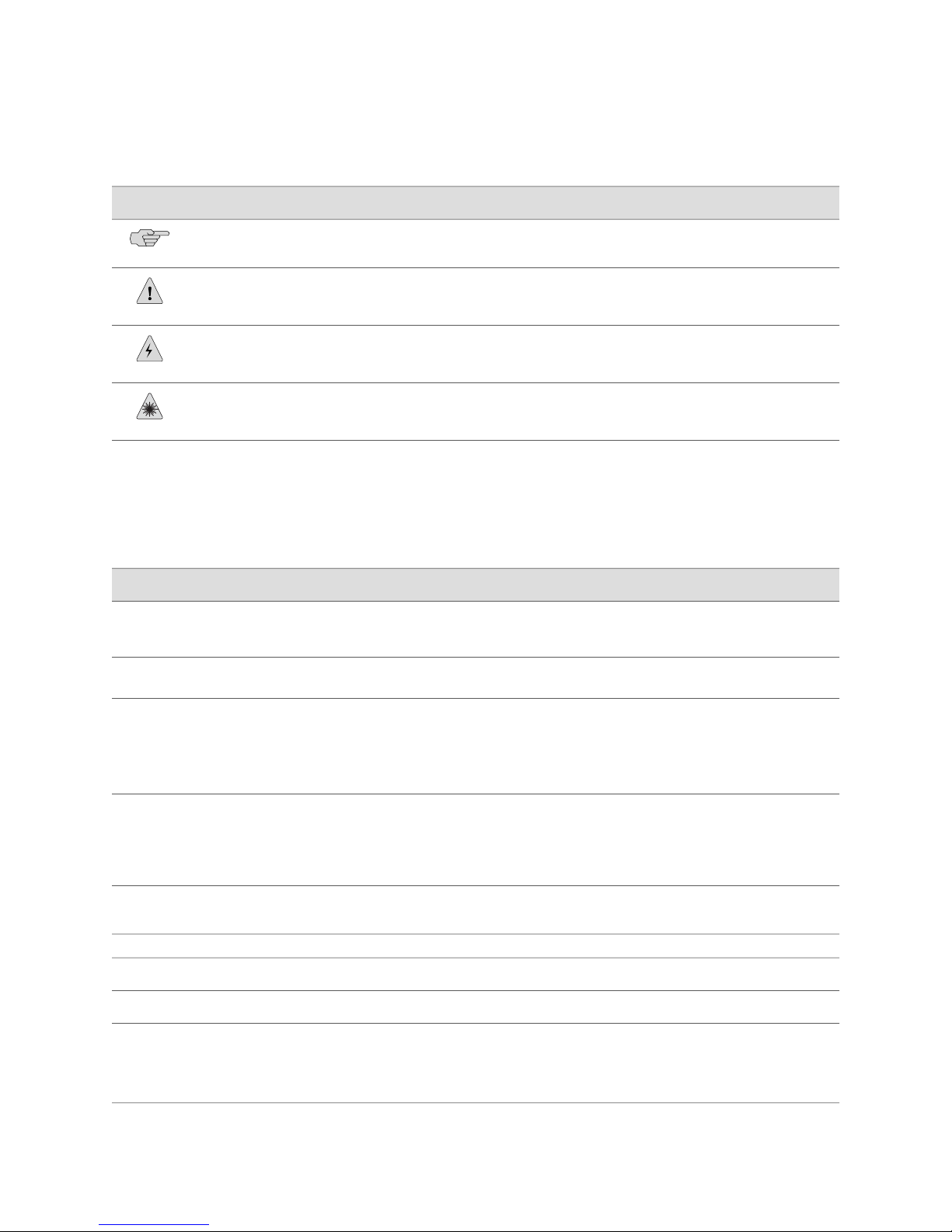
Table 1: Notice Icons

Table 2 on page xxx defines text and syntax conventions that we use throughout the
E Series and JUNOSe documentation.

DescriptionMeaningIcon

Indicates important features or instructions.Informational note

Indicates a situation that might result in loss of data or hardware damage.Caution

Alerts you to the risk of personal injury or death.Warning

Alerts you to the risk of personal injury from a laser.Laser warning

Table 2: Text and Syntax Conventions

Represents commands and keywords in text.Bold text like this

Bold text like this

Fixed-width text like this

Represents text that the user must type.

Represents information as displayed on your
terminal’s screen.

Italic text like this

Emphasizes words.

■

Identifies variables.

■

Identifies chapter, appendix, and book

■

names.

Plus sign (+) linking key names

keys simultaneously.

Syntax Conventions in the Command Reference Guide

ExamplesDescriptionConvention

Issue the clock source command.

■

Specify the keyword exp-msg.

■

host1(config)#traffic class low-loss1

host1#show ip ospf 2

Routing Process OSPF 2 with Router
ID 5.5.0.250
Router is an Area Border Router
(ABR)

There are two levels of access: user and

■

privileged.

clusterId, ipAddress.

■

Appendix A, System Specifications

■

Press Ctrl + b.Indicates that you must press two or more

terminal lengthRepresents keywords.Plain text like this

| (pipe symbol)

xxx ■ E Series and JUNOSe Text and Syntax Conventions

mask, accessListNameRepresents variables.Italic text like this

diagnostic | lineRepresents a choice to select one keyword
or variable to the left or to the right of this
symbol. (The keyword or variable can be
either optional or required.)

Table 2: Text and Syntax Conventions (continued)

About the Documentation

ExamplesDescriptionConvention

[ internal | external ]Represent optional keywords or variables.[ ] (brackets)

[ ]* (brackets and asterisk)

that can be entered more than once.

Represent required keywords or variables.{ } (braces)

Obtaining Documentation

To obtain the most current version of all Juniper Networks technical documentation,
see the Technical Documentation page on the Juniper Networks Web site at

http://www.juniper.net/.

To download complete sets of technical documentation to create your own
documentation CD-ROMs or DVD-ROMs, see the Offline Documentation page at

http://www.juniper.net/techpubs/resources/cdrom.html

Copies of the Management Information Bases (MIBs) for a particular software release
are available for download in the software image bundle from the Juniper Networks
Web site athttp://www.juniper.net/.

Documentation Feedback

[ level1 | level2 | l1 ]*Represent optional keywords or variables

{ permit | deny } { in | out }

{ clusterId | ipAddress }

We encourage you to provide feedback, comments, and suggestions so that we can
improve the documentation to better meet your needs. Send your comments to

[e-mail], or fill out the documentation feedback form at

https://www.juniper.net/cgi-bin/docbugreport/. If you are using e-mail, be sure to include

the following information with your comments:

■ Document or topic name

■ URL or page number

■ Software release version

Requesting Technical Support

Technical product support is available through the Juniper Networks Technical
Assistance Center (JTAC). If you are a customer with an active J-Care or JNASC support
contract, or are covered under warranty, and need post-sales technical support, you
can access our tools and resources online or open a case with JTAC.

■ JTAC policies—For a complete understanding of our JTAC procedures and policies,

review the JTAC User Guide located at

http://www.juniper.net/customers/support/downloads/7100059-EN.pdf .

Obtaining Documentation ■ xxxi

JUNOSe 11.1.x Quality of Service Configuration Guide

■ Product warranties—For product warranty information, visit

http://www.juniper.net/support/warranty/ .

■ JTAC hours of operation—The JTAC centers have resources available 24 hours a

day, 7 days a week, 365 days a year.

Self-Help Online Tools and Resources

For quick and easy problem resolution, Juniper Networks has designed an online
self-service portal called the Customer Support Center (CSC) that provides you with
the following features:

■

Find CSC offerings: http://www.juniper.net/customers/support/

■

Search for known bugs: http://www2.juniper.net/kb/

■

Find product documentation: http://www.juniper.net/techpubs/

■ Find solutions and answer questions using our Knowledge Base:

http://kb.juniper.net/

■ Download the latest versions of software and review release notes:

http://www.juniper.net/customers/csc/software/

■ Search technical bulletins for relevant hardware and software notifications:

https://www.juniper.net/alerts/

■ Join and participate in the Juniper Networks Community Forum:

http://www.juniper.net/company/communities/

■

Open a case online in the CSC Case Management tool: http://www.juniper.net/cm/

To verify service entitlement by product serial number, use our Serial Number
Entitlement (SNE) Tool: https://tools.juniper.net/SerialNumberEntitlementSearch/

Opening a Case with JTAC

You can open a case with JTAC on the Web or by telephone.

■

Use the Case Management tool in the CSC at http://www.juniper.net/cm/ .

■ Call 1-888-314-JTAC (1-888-314-5822 toll-free in the USA, Canada, and Mexico).

For international or direct-dial options in countries without toll-free numbers, see

http://www.juniper.net/support/requesting support.html .

xxxii ■ Requesting Technical Support

Part 1

QoS on the E Series Router

■ Quality of Service Overview on page 3

QoS on the E Series Router ■ 1

JUNOSe 11.1.x Quality of Service Configuration Guide

2 ■ QoS on the E Series Router

Chapter 1

Quality of Service Overview

The quality of service (QoS) feature enables your E Series router to distinguish traffic
with strict timing requirements from traffic that can tolerate delay, jitter, and loss.

QoS topics are discussed in the following sections:

■ QoS on the E Series Router Overview on page 3

■ QoS Audience on page 4

■ QoS Platform Considerations on page 4

■ QoS Terms on page 5

■ QoS Features on page 7

■ Configuring QoS on the E Series Router on page 8

■ QoS References on page 9

QoS on the E Series Router Overview

QoS is a suite of features that configure queuing and scheduling on the forwarding
path of the Juniper Networks E Series Broadband Services Routers. QoS provides a
level of predictability and control beyond the best-effort delivery that the router
provides by default. Best-effort service provides packet transmission with no assurance
of reliability, delay, jitter, or throughput.

QoS as developed for E Series routers conforms to the IETF Differentiated Services
(DiffServ) model (RFCs 2597 and 2598). DiffServ networks classify packets into one
of a small number of aggregated flows or traffic classes for which you can configure
different QoS characteristics. The Juniper Networks QoS architecture extends DiffServ
to support edge features such as high-density queuing.

The E Series router supports:

■ IETF architecture for differentiated services

■ Assured forwarding per-hop-behavior (PHB) groups

■ Expedited forwarding PHB groups

The router supports configurable queuing and scheduling. It has an application-specific
integrated circuit (ASIC) scheduler that supports thousands of queues in a hierarchical
round-robin (HRR) scheduler. The scheduler allows the router to allocate separate

QoS on the E Series Router Overview ■ 3

E Series router

JUNOSe 11.1.x Quality of Service Configuration Guide

queues for each forwarding interface. Separate queues enable fair access to buffers
and bandwidth for each subscriber connected to the router.

Allocating queues per interface allows an Internet service provider (ISP) to shape an
individual subscriber’s traffic flows to specified rates independent of the underlying
Layer 2 network type.

Related Topics ■ For a list of related RFCs, see Configuring QoS on the E Series Router on page 8

QoS Audience

This topic collection contains configuration information for two types of QoS users:
QoS administrators and QoS clients.

QoS administrators are responsible for implementing a QoS queuing architecture by
defining drop profiles, queue profiles, scheduler profiles, QoS profiles, and QoS
parameter definitions.

QoS clients are responsible for configuring services for individual subscribers by
creating parameter instances. The parameter instances that QoS clients can create
depend on the settings defined in parameter definitions by the QoS administrator.

Related Topics ■ For information about QoS users and QoS parameters, see QoS Parameter

Audience on page 225

QoS Platform Considerations

QoS is supported on all E Series line modules except for the ES2 10G Uplink LM.

Figure 1 on page 4 shows the traffic flow through the router.

Figure 1: Traffic Flow Through an E Series Router

For information about the modules supported on E Series routers:

■ See the ERX Module Guide for modules supported on ERX7xx models, ERX14xx

models, and the Juniper Networks ERX310 Broadband Services Router.

■ See the E120 and E320 Module Guide for modules supported on the Juniper

Networks E120 and E320 Broadband Services Routers.

4 ■ QoS Audience

Interface Specifiers

Chapter 1: Quality of Service Overview

The majority of the configuration task examples in this topic collection use the slot/port
format to specify an interface. However, the interface specifier format that you use
depends on the router that you are using.

For ERX7xx models, ERX14xx models, and ERX310 routers, use the slot/port format.
For example, the following command specifies an ATM interface on slot 0, port 1 of
an ERX7xx model, ERX14xx model, or ERX310 router.

host1(config)#interface gigabitEthernet 0/1

For E120 and E320 routers, use the slot/adapter/port format, which includes an
identifier for the bay in which the I/O adapter (IOA) resides. In the software, adapter
0 identifies the right IOA bay (E120 router) and the upper IOA bay (E320 router);
adapter 1 identifies the left IOA bay (E120 router) and the lower IOA bay (E320
router). For example, the following command specifies a10-Gigabit Ethernet interface
on slot 5, adapter 0, port 0 of an E320 router.

Related Topics ■ For more information about supported interface types and specifiers on E Series

QoS Terms

host1(config)#interface tenGigabitEthernet 5/0/0

routers, see Interface Types and Specifiers.

Table 3 on page 5 defines terms used in this discussion of QoS.

Table 3: QoS Terminology

DescriptionTerm

Assured rate

Best effort

Best-effort queue

Best-effort scheduler node

Bandwidth guaranteed until the node below in the scheduler
hierarchy is oversubscribed.

Network forwards as many packets as possible in as reasonable a
time as possible. This is the default per-hop behavior (PHB) for packet
transmission.

For a logical interface, the queue associated with the best-effort
traffic class for that logical interface,

The scheduler node associated with a logical interface and traffic
class group pair, and where the traffic class group contains the
best-effort traffic class. Also known as best-effort node.

CDV

CDVT

Cell delay variation. Measures the difference between a cell’s
expected and actual transfer delay. Determines the amount of jitter.

Cell delay variation tolerance. Specifies the acceptable tolerance of
CDV (jitter).

QoS Terms ■ 5

JUNOSe 11.1.x Quality of Service Configuration Guide

Table 3: QoS Terminology (continued)

DescriptionTerm

Effective weight

Group node

HAR

HRR

Latency

Management Information
Base (MIB)

Queue

QoS port-type profile

The result of a weight or an assured rate. Users configure the
scheduler node by specifying either an assured rate or a weight
within a scheduler profile. An assured rate, in bits per second, is
translated into a weight. The resultant weight is referred to as an
effective weight.

A scheduler node associated with a {port interface, traffic-class
group} pair. Because the logical interface is the port, only one such
scheduler node can exist for each traffic-class group above the port.
This node aggregates all traffic for traffic classes in the group.

Hierarchical assured rate. Dynamically adjusts bandwidth for
scheduler nodes.

Hierarchical round-robin. Allocates bandwidth to queues in
proportion to their weights.

Delay in the transmission of a packet through a network from
beginning to end.

Supported on the E Series router.Proprietary QoS

First-in-first-out (FIFO) set of buffers that control packets on the data
path.

Supplies the QoS information for forwarding interfaces stacked above
ports of the associated interface type.

Scheduler hierarchy

Scheduler node

Shared shaper constituent

Applies the rules in the QoS profile to a specific interface.QoS profile attachment

Allows you to throttle a queue to a specified rate.Rate shaping

Random early detection congestion avoidance technique.RED

A hierarchical, tree-like arrangement of scheduler nodes and queues.
The router supports up to three levels of scheduler nodes stacked
above a port. The port scheduler is at level 0, with two levels of
scheduler nodes at levels 1 and 2. A final level of queues is stacked
above the nodes.

An element within the hierarchical scheduler that implements
bandwidth controls for a group of queues. Queues are stacked above
scheduler nodes in a hierarchy. The root node is associated with a
channel or physical port.

Bandwidth in a queue or node can be throttled to a specified rate.Shaping rate

All nodes and queues that are associated with a logical interface that
is being shared shaped are considered potential constituents of the
shared shaper.

Specifies the relative weight for queues in the traffic class.Weight

6 ■ QoS Terms

QoS Features

Chapter 1: Quality of Service Overview

Table 3: QoS Terminology (continued)

DescriptionTerm

Weighted random early detection congestion avoidance technique.WRED

Table 4 on page 7 describes the major QoS features supported on the E Series
router.

Table 4: QoS Features

DescriptionFeature

Best effort

Differentiated services

Drop profile

Port shaping

QoS parameters

QoS port-type profile

QoS profile

Queue profile

Default traffic class for packets being forwarded across the device.
Packets that are not assigned to a specific traffic class are assigned
to the best-effort traffic class.

Assured forwarding—See RFC 2597.

■

Expedited forwarding—See RFC 2598.

■

Template that specifies active queue management in the form of
WRED behavior of an egress queue.

Shapes the aggregate traffic through a port or channel to a rate that
is less than the line or port rate.

Creates a queuing architecture without the numeric subscriber rates
and weights in scheduler profiles. You then use the same QoS and
scheduler profiles across all subscribers who use the same services
but at different bandwidths, reducing the total number of QoS
profiles and scheduler profiles required.

QoS profile that is automatically attached to ports of the
corresponding type if you do not explicitly attach a QoS profile.

Collection of QoS commands that specify queue profiles, drop
profiles, scheduler profiles, and statistics profiles in combination
with interface types.

Template that specifies the buffering and tail-dropping behavior of
an egress queue.

Rate shaping

Mechanism that throttles the rate at which an interface can transmit
packets.

Note: Rate shaping as presented in policy management in releases
before JUNOSe Release 4.0 is deprecated and converted to QoS
profiles and scheduler profiles.

QoS Features ■ 7

JUNOSe 11.1.x Quality of Service Configuration Guide

Table 4: QoS Features (continued)

DescriptionFeature

Relative strict-priority
scheduling

Scheduler profile

Shared rate shaping

Statistics profile

Strict-priority scheduling

Traffic class

Provides strict-priority scheduling within a shaped aggregate rate.
For example, it lets you provide 1 Mbps of aggregate bandwidth to
a subscriber, with up to 500 Kbps of the bandwidth for low-latency
traffic. If there is no strict-priority traffic, the low-latency traffic can
use up to the full aggregate rate of 1 Mbps.

Configures the bandwidth at which queues drain as a function of
relative weight, assured rate, and shaping rate.

Mechanism for shaping a logical interface's aggregate traffic to a
rate when the traffic for that logical interface is queued through
more than one scheduler hierarchy.

Template that specifies rate statistics and event-gathering
characteristics.

Designates the traffic class (queue) that receives top priority for
transmission of its packets through a port. It is implemented with
a special strict-priority scheduler node that is stacked directly above
the port.

A chassis-wide grouping of queues and buffers that support
transmission of a designated set of traffic across the chassis, from
ingress line module, through the switch fabric, and onto the egress
line module.

The router supports up to eight traffic classes, and therefore up to
eight queues per logical interface.

Traffic-class group

WRED

Separate hierarchy of scheduler nodes and queues over a port. A
traffic-class group uses one level of the scheduler hierarchy, level

1.

Traffic classes belong to the default group unless they are specifically
assigned to a named group. All queues are stacked in a single
scheduler hierarchy above the physical port. When you configure
a traffic class inside a group, its queues are stacked separately. The
most common reason for creating separate scheduler hierarchies
is to implement strict priority scheduling for all queues in the group.

The router supports up to four traffic-class groups. A traffic class
cannot belong to more than one group.

Signals end-to-end protocols such as TCP that the router is becoming
congested along a particular egress path. The intent is to trigger
TCP congestion avoidance in a random set of TCP flows before
congestion becomes severe and causes tail dropping on a large
number of flows.

Configuring QoS on the E Series Router

Several of the tasks for configuring QoS on your E Series router are optional.

8 ■ Configuring QoS on the E Series Router

Chapter 1: Quality of Service Overview

To configure QoS on your E Series router:

1. Create and configure a traffic class.

See “Traffic Class and Traffic-Class Groups Overview” on page 13.

2. (Optional) Create one or more traffic-class groups.

See “Traffic Class and Traffic-Class Groups Overview” on page 13.

3. (Optional) To configure nondefault buffer management, create a queue profile.

See “Queuing and Buffer Management Overview” on page 17.

4. (Optional) To configure RED or WRED, create a drop profile.

See “Dropping Behavior Overview” on page 25.

5. (Optional) To gather rate statistics, create a statistics profile.

See “QoS Statistics Overview” on page 37.

6. Configure a scheduler hierarchy with a scheduler profile.

QoS References

See “Scheduler Hierarchy Overview” on page 45.

7. (Optional) Configure shaping:

■ Configure shaping and shared shaping using the scheduler profile.

See “Rate Shaping and Port Shaping Overview” on page 51, “Simple Shared
Shaping Overview” on page 79, and “Compound Shared Shaping Overview”
on page 99.

■ Configure shaping rates independent of the QoS profile and scheduler profile

using QoS parameters.

See “Parameter Definition Attributes for QoS Administrators Overview” on
page 229.

8. Create a QoS profile. QoS profiles reference queue, drop, statistics, and scheduler

profiles.

See “Queuing and Buffer Management Overview” on page 17.

9. Attach the QoS profile to one or more interfaces, or specify the profile as a QoS

port-type profile for a given interface type.

See “Queuing and Buffer Management Overview” on page 17.

For more information about QoS, see the following resources:

■ RFC 2474—Definition of the Differentiated Services Field (DS Field) in the IPv4

and IPv6 Headers (December 1998)

■ RFC 2475—An Architecture for Differentiated Services (December 1998)

■ RFC 2597—Assured Forwarding PHB Group (June 1999)

■ RFC 2598—An Expedited Forwarding PHB (June 1999)

■ RFC 2698—A Two Rate Three Color Marker (September 1999)

QoS References ■ 9

JUNOSe 11.1.x Quality of Service Configuration Guide

■ RFC 2990—Next Steps for the IP QoS Architecture (November 2000)

■ RFC 2998—A Framework for Integrated Services Operation over Diffserv

Networks (November 2000)

■ RFC 3246—An Expedited Forwarding PHB (Per-Hop Behavior) (March 2002)

■ RFC 3260—New Terminology and Clarifications for Diffserv (April 2002)

■ DSL Forum Technical Report (TR)-059—DSL Evolution - Architecture

Requirements for the Support of QoS-Enabled IP Services

■ Floyd, S., and Jacobson, V. Random Early Detection for Congestion Avoidance.

IEEE/ACM Transactions on Networking 1(4), August 1993

10 ■ QoS References

Part 2

Classifying, Queuing, and Dropping Traffic

■ Defining Service Levels with Traffic Classes and Traffic-Class Groups on page 13

■ Configuring Queue Profiles for Buffer Management on page 17

■ Configuring Dropping Behavior with RED and WRED on page 25

■ Gathering Statistics for Rates and Events in the Queue on page 37

Classifying, Queuing, and Dropping Traffic ■ 11

JUNOSe 11.1.x Quality of Service Configuration Guide

12 ■ Classifying, Queuing, and Dropping Traffic

Chapter 2

Defining Service Levels with Traffic
Classes and Traffic-Class Groups

This chapter provides information for configuring traffic classes and traffic-class
groups on the E Series router.

QoS topics are discussed in the following sections:

■ Traffic Class and Traffic-Class Groups Overview on page 13

■ Configuring Traffic Classes That Define Service Levels on page 14

■ Configuring Traffic-Class Groups That Define Service Levels on page 15

■ Monitoring Traffic Classes and Traffic-Class Groups for Defined Levels of

Service on page 16

Traffic Class and Traffic-Class Groups Overview

A traffic class is a systemwide collection of buffers, queues, and bandwidth that you
can allocate to provide a defined level of service to packets in the traffic class.

A traffic class corresponds to what the IETF DiffServ working group calls a traffic
class in RFC 2597—Assured Forwarding PHB Group (June 1999).

Traffic classes are global to the router. Packets are:

■ Classified into a traffic class on ingress or egress by input policies

■ Queued on fabric queues that are specific to the traffic class

■ Queued on the egress line module on queues that are specific to the traffic class

■ Scheduled for transmission by the scheduler

Best-Effort Forwarding

The router has a default traffic class called best-effort. You cannot delete this class.
You can add the best-effort class to a traffic-class group. The router assigns packets
to the best-effort class in each of the following cases:

■ You do not create any other traffic classes.

■ Packets are not classified into a traffic class.

Traffic Class and Traffic-Class Groups Overview ■ 13

JUNOSe 11.1.x Quality of Service Configuration Guide

■ Packets arrive at an egress line module that has no queues allocated for their

traffic class.

Traffic-Class Groups Overview

You can put traffic classes into a group to create a hierarchy of scheduler nodes and
queues. Organizing traffic into multiple traffic-class groups enables you to manage
and shape traffic—by service class, for example—when the traffic classes are
distributed across different VCs. A traffic-class group contains one or more traffic
classes, but a particular traffic class can belong only to a single group—either the
default group or one named group.

You can configure an auto-strict group and up to three extended traffic-class groups.
You must put traffic classes that require strict-priority scheduling in the auto-strict
group. You can optionally put traffic classes that need a separate round robin (for
example, video) in an extended group.

A traffic class that is not contained in any named group is considered to belong to
the default group. Traffic classes are placed in the default traffic-class group when
the classes are configured—you can then move a class to another traffic-class group.
When you delete a traffic-class from a named group, the class is automatically moved
to the default traffic-class group. ATM VC nodes that are configured in the default
group (which is the factory default configuration) receive backpressure from the
segmentation and reassembly (SAR) feature in the default qos-mode-port node.

Traffic-class groups are global in scope by default. However, you might want to
manage certain traffic classes through particular line modules. If you have already
created a traffic-class group, you can subsequently specify a slot number to create
a local instance of the group that is restricted to the module occupying that slot.
Characteristics configured for the local group on the line module override those of
the global group, for only that line module. Traffic classes in a globally scoped
traffic-class group cannot belong to any other group. Traffic classes in a local
traffic-class group cannot belong to any other group.

Related Topics Configuring Traffic Classes That Define Service Levels on page 14■

■ Configuring Traffic-Class Groups That Define Service Levels on page 15

Configuring Traffic Classes That Define Service Levels

The router supports up to eight global traffic classes. Each traffic class can appear in
only one traffic-class group. If not explicitly added to a traffic-class group, the traffic
class is considered to be ungrouped.

To configure a traffic class:

1. Create a traffic class by assigning a name that represents the type of service and

enter Traffic Class Configuration mode.

14 ■ Configuring Traffic Classes That Define Service Levels

host1(config)#traffic-class low-loss1
host1(config-traffic-class)#

Chapter 2: Defining Service Levels with Traffic Classes and Traffic-Class Groups

The traffic class name can be up to 31 characters. It cannot include spaces.

2. (Optional) Specify strict-priority scheduling across the fabric for queues in the

traffic class.

host1(config-traffic-class)#fabric-strict-priority

3. (Optional) For Juniper Networks ERX1440, E120 , and E320 Broadband Services

Routers, specify the relative weight for queues in the traffic class in the fabric.

host1(config-traffic-class)#fabric-weight 12

Fabric weight controls the bandwidth of fabric queues associated with the traffic
class. It does not control the weight of egress queues associated with the traffic
class. If multiple traffic classes are strict priority, the fabric weight determines
which class gets more bandwidth.

The weight value is in the range 1–63. The default is 8. Zero is not a valid weight.

Related Topics ■ Monitoring Traffic Classes and Traffic-Class Groups for Defined Levels of Service

on page 16

■ fabric-strict-priority

■ fabric-weight

■ traffic-class

Configuring Traffic-Class Groups That Define Service Levels

You can configure a traffic-class group and enter Traffic Class Group Configuration
mode, from which you can add classes to or delete classes from the group.

Each traffic class can appear in only one traffic-class group. If not explicitly added
to a traffic-class group, the traffic class is considered to be ungrouped.

To configure a traffic-class group:

1. Create a traffic-class group by assigning a name that represents the type of service

and enter Traffic Class Group Configuration mode.

host1(config)#traffic-class-group assured slot 9 extended
host1(config-traffic-class-group)#

The traffic class name can be up to 31 characters. It cannot include spaces.

If you do not specify a keyword, the group is strict-priority by default.

You can use the auto-strict-priority keyword to explicitly configure a single
traffic-class group with strict-priority scheduling, regardless of the scheduler
profile associated with the group node.

You can use the extended keyword to configure up to three extended traffic-class
groups. Scheduling for these groups is determined by the scheduler profile
associated with the group node. If an explicitly configured strict-priority group

Configuring Traffic-Class Groups That Define Service Levels ■ 15

JUNOSe 11.1.x Quality of Service Configuration Guide

exists, the scheduler for the extended groups may not specify strict-priority
scheduling.

Use the slot slotNumber option to associate a pre-existing global traffic-class
group with the module occupying that slot. Characteristics configured for the
local group on the line module override those of the global group.

2. Add traffic classes to the traffic-class group.

host1(config-traffic-class-group)#traffic-class low-latency-traffic-class

Related Topics ■ Configuring Traffic Classes That Define Service Levels on page 14

■ Monitoring Traffic Classes and Traffic-Class Groups for Defined Levels of Service

on page 16

■ traffic-class

■ traffic-class-group

Monitoring Traffic Classes and Traffic-Class Groups for Defined Levels of Service

To monitor traffic classes and traffic-class groups:

■ Monitoring Service Levels with Traffic Classes on page 314

■ Monitoring Service Levels with Traffic-Class Groups on page 315

16 ■ Monitoring Traffic Classes and Traffic-Class Groups for Defined Levels of Service

Chapter 3

Configuring Queue Profiles for Buffer
Management

This chapter provides information for configuring queue profiles for buffer
management on the E Series router.

QoS topics are discussed in the following sections:

■ Queuing and Buffer Management Overview on page 17

■ Memory Requirements for Queue and Buffers on page 19

■ Guidelines for Managing Queue Thresholds on page 19

■ Guidelines for Managing Buffers on page 20

■ Configuring Queue Profiles to Manage Buffers and Thresholds on page 22

■ Monitoring Queues and Buffers on page 24

Queuing and Buffer Management Overview

A queue is a set of first-in, first-out (FIFO) buffers that buffer packets on the data
path. QoS associates queues with a traffic class/interface pair. For example, if you
create 4000 IP interfaces and configure each interface with four traffic classes, then
16,000 queues are created. For specific information about the maximum number
of QoS queues supported, see JUNOSe Release Notes, Appendix A, System Maximums.

The E Series router dynamically manages the shared memory on egress line modules
to provide a good balance between sharing the memory among queues and protecting
an individual queue’s claim on its fair share of the egress memory.

When egress packet memory is in high demand and aggregate utilization of the
packet memory is high, queue lengths are set to lengths that strictly partition egress
memory into per-queue memory sections. This conservative buffer-management
strategy reserves a fair share of buffers for each queue, so that high bandwidth
consumers cannot starve out moderate traffic consumers by allocating all the shared
memory resource for themselves.

When egress packet memory is in low demand, a more liberal buffer management
strategy is used to provide active queues with more access to the shared memory
resource.

Queuing and Buffer Management Overview ■ 17

JUNOSe 11.1.x Quality of Service Configuration Guide

The router dynamically varies queue lengths for all queues as the real-time demand
on the egress packet memory changes. You can configure limits to prevent the router
from setting queue lengths too low or too high.

Static Oversubscription

The router uses static oversubscription to vary queue thresholds based on the number
of queues currently configured, which is relatively static. Static oversubscription is
based on the assumption that, when a few queues are configured, many of the queues
are likely to be active at the same time. When a large number of queues are
configured, fewer queues are likely to be active at the same time.

When few queues are configured, buffer memory is strictly partitioned between
queues to ensure that buffers are available for all queues. As the number of configured
queues increases, buffer memory is increasingly oversubscribed to allow more buffer
sharing. Reserving buffer space for all queues when many are expected to be idle is
unnecessary and wasteful.

Dynamic Oversubscription

The router uses dynamic oversubscription to vary queue thresholds based on the
amount of egress buffer memory in use. The router divides egress buffer memory
into eight regions.

The size of the region depends on the ASIC type. For more information, see “Memory
Requirements for Queue and Buffers” on page 19.

When buffer memory is in low demand, queues are given large amounts of buffer
memory. As the demand for buffer memory increases, queues are given progressively
smaller amounts of buffer memory.

Color-Based Thresholding

Packets within the router are tagged with a drop precedence:

■ Committed—Green

■ Conformed—Yellow

■ Exceeded—Red

When the queue fills above the exceeded threshold, the router drops red packets,
but still queues yellow and green packets. When the queue fills above the conformed
drop threshold, the router queues only green packets.

NOTE: All color-based thresholds vary in proportion to the dynamic queue length.

Related Topics ■ Configuring Queue Profiles to Manage Buffers and Thresholds on page 22

■ Guidelines for Managing Queue Thresholds on page 19

18 ■ Queuing and Buffer Management Overview

Chapter 3: Configuring Queue Profiles for Buffer Management

■ Guidelines for Managing Buffers on page 20

■ RED and WRED Overview on page 26

Memory Requirements for Queue and Buffers

JUNOSe software uses 128-byte buffers.

The egress memory available for queues available depends on the ASIC and the line
module. Table 5 on page 19 lists the egress memory.

Table 5: Egress Memory and Region Size on ASIC Line Modules

Egress Memory
(MB)Line ModuleASIC

Region Size (MB)

Related Topics To identify the type of ASIC used by a line module, see the ERX Module Guide

■

and the E120 and E320 Module Guide

■ Guidelines for Managing Queue Thresholds on page 19

■ Guidelines for Managing Buffers on page 20

Guidelines for Managing Queue Thresholds

To prevent the router from setting queue thresholds too low or too high, you can
specify minimum and maximum queue thresholds. You can also specify the
conformed length and exceeded length as percentages of the committed length.

Guidelines for Configuring a Maximum Threshold

432All EFA line modulesEFA

864GE-2 and GE-HDEFFA

16128OC48

16128ES2 4G LM

1296ES2 10G LMTFA

We recommend that you constrain queue thresholds using committed or conformed
threshold settings; any unused memory is redistributed to queues whose thresholds
are not constrained. This use of thresholds is analogous to the way that shaping rates
constrain bandwidth and cause bandwidth redistribution to unconstrained queues.

For example, voice queues are scheduled at strict priority; therefore, they require
very little buffering. Configuring a maximum queue threshold enables the system to
allocate more buffers to other queues in the system. Video queues are similar but

Memory Requirements for Queue and Buffers ■ 19

JUNOSe 11.1.x Quality of Service Configuration Guide

because they are higher bandwidth, they might require higher maximum committed
thresholds.

You might want to limit latency of your multicast traffic by bounding the queue length
using a maximum committed threshold. The following example configures the
multicast queues so that the committed threshold never exceeds 20 KB, even when
the egress memory is lightly loaded. The forfeited buffers are allocated to other
queues.

host1(config)#queue-profile multicast
host1(config-queue)#committed-length 0 20000
host1(config-queue)#exit

Be sure to include 0 in the syntax, or you will configure a minimum threshold.

Guidelines for Configuring a Minimum Threshold

Configuring a minimum threshold does not guarantee that a queue always obtains
the minimum buffer allocation. You can configure 1000 queues with a minimum of
1 MB each, but the buffer memory is 32 MB or 128 MB, not 1 GB. In this case, the
system moves into higher operating regions (global utilization) if all these queues
buffer traffic, until it reaches 90 percent utilization. At that point, the thresholds must
reduce to the reserved percentages, and the queue thresholds drop from a high
threshold to a very low one. Queues are not guaranteed to obtain any buffering, and
are buffered in the order in which they are received.

You can configure a minimum committed threshold by specifying a value such as
1000 with the committed-length command:

host1(config)#queue-profile multicast
host1(config-queue)#committed-length 1000 20000
host1(config-queue)#exit

Related Topics Memory Requirements for Queue and Buffers on page 19■

■ Configuring Queue Profiles to Manage Buffers and Thresholds on page 22

Guidelines for Managing Buffers

Queue profiles enable you to manage queue thresholds and buffers to manage the
following common problems:

■ Queues that back up and consume too many buffers

■ Queues that cannot obtain buffers when they need them (called buffer starvation)

You can set the buffer weight to ensure that some sets of queues get higher thresholds
than others. Buffer weight is analogous to weight in a scheduler profile. It directs the
router to set the queue thresholds proportionately.

20 ■ Guidelines for Managing Buffers

Chapter 3: Configuring Queue Profiles for Buffer Management

This feature provides graceful buffer allocation as the global utilization goes higher;
queues with more buffer weight always obtain more buffers, but they do not undergo
a dramatic drop in threshold when the system moves from region to region.

JUNOSe software uses 128-byte buffers. When setting very small queue thresholds,
keep the following guidelines in mind:

■ Specifying a maximum queue length of 0 bytes disables queuing of packets on

the queue.

■ Specifying a maximum queue length of 1–128 bytes creates a single 128-byte

buffer for the queue.

■ Specifying a maximum queue length of 129–256 bytes creates two 128-byte

buffers for the queue.

■ Packets and cells consume at least one buffer.

For example, a 64-byte packet consumes a single 128-byte buffer. If you specify
a maximum queue length of 256 bytes, then either two packets of 64–128 bytes
in length or a single packet of 129–256 bytes can be queued.

For example, suppose a line module with 4000 IP interfaces is configured with four
queues per IP interface, corresponding to four traffic classes. Suppose that queues
in two of the traffic classes are configured with a buffer weight of 24 to increase burst
tolerance. The following example configures the video queue:

host1(config)#queue-profile video
host1(config-queue)#buffer-weight 24
host1(config-queue)#exit
host1(config)#

When the egress memory is fully loaded, dynamic oversubscription is 0 percent, and
the 8000 queues with the default buffer weight strictly partition 25 percent of the
32-MB memory, leaving 75 percent of the memory for the queues weighted 24
(corresponding to the ratio 75 percent:25 percent, or 24:8). Therefore, these queues
have committed thresholds of 1 KB each, and queues with the buffer weight of 24
have committed thresholds of 3 KB each. As the egress memory becomes
progressively less loaded, all the queue thresholds increase proportionally, based on
dynamic oversubscription, but the queues with buffer weight 24 are always set with
thresholds three times larger than the default thresholds.

Guidelines for Managing Buffer Starvation

Buffer starvation most commonly occurs when queues or nodes exist in a large round
robin, usually in the default traffic-class group. When the round robin congests, the
queues back up and require more buffers. The traffic in the round robin starts to
burst based on a single node or queue. After a packet is dequeued, the node or queue
can wait for thousands of other queues to dequeue a packet before it can dequeue
again. During this time, the queue backs up.

If you configure different scheduler profile weights or assured rates for nodes in a
large and congested round robin, the buffer starvation becomes apparent. The
problem occurs when the heavy weighted nodes wait their turn in the round robin
and thousands of other nodes dequeue. While the heavily weighted nodes wait, the

Guidelines for Managing Buffers ■ 21

JUNOSe 11.1.x Quality of Service Configuration Guide

system needs to buffer them. However, all queues receive the same buffer allocation
by default. If the system goes to higher buffer regions, it starts dropping packets for
all queues. When the heavy weight node finally transmits, it dequeues all buffers,
but it cannot dequeue the packets that were dropped. You do not achieve the expected
bandwidth based on scheduler profile weights.

To manage buffer starvation, configure buffer weights on queues so they are in the
same ratio as the expected bandwidth for the queues. For example, if two queues
have scheduler weight (or assured-rate) in the ratio of 2:1, then set the buffer weights
to the same ratio.

To manage buffer starvation, set the maximum-committed-threshold on queues
that do not need buffering, and increase the buffer-weight for the heavily weighted
queues in the round robin.

The system calculates the correct ratio for you. Issue the show egress queue rates
command to see the ratio:

host1# show egress-queue rates brief interface fastEthernet 9/0.2
traffic forwarded aggregate minimum maximum
interface class rate drop rate rate rate

---------------------- ----------------------- --------- --------- ------- ------­ip FastEthernet9/0.2 best-effort 0 0 25000 1000000
videoTrafficClass 0 0 375000 1000000
multicastTrafficClass 0 0 925000 1000000
internetTrafficClass 0 0 50000 1000000
Total: 0 0

Queues reported: 4
Queues filtered (under threshold): 0
Queues disabled (no rate period): 0
Queues disabled (no resources): 0
Total queues: 4

The minimum rate for each queue is the approximate rate the queue achieves if all
configured queues in the line module run infinite traffic. Configure the buffer weights
in proportion to the minimum rate displayed by the system.

Related Topics Memory Requirements for Queue and Buffers on page 19■

■ Configuring Queue Profiles to Manage Buffers and Thresholds on page 22

■ Monitoring Forwarding and Drop Rates on the Egress Queue on page 333

Configuring Queue Profiles to Manage Buffers and Thresholds

A queue profile controls the buffering and dropping behavior of a set of egress queues
by enabling you to set the buffer weight of the queue, the drop thresholds, and the
constraints on queue lengths.

Set the queue lengths as follows:

■ To oversubscribe buffer memory, set a minimum queue length.

22 ■ Configuring Queue Profiles to Manage Buffers and Thresholds

Chapter 3: Configuring Queue Profiles for Buffer Management

NOTE: If the sum of the queue minimum lengths is greater than the amount of
egress buffer memory, then the egress buffer memory is oversubscribed.

■ To configure a minimal level of buffering or to limit the buffering in queues, set

a maximum queue length. For example, if you want to control latency by
configuring very small queues, set the maximum queue length to 256 bytes. The
system queues no more than 256 bytes.

If you do not set the queue lengths, the router varies the queue length dynamically
in the range 1 KB–7 MB.

1. Create a queue profile and enter Queue Configuration mode.

host1(config)#queue-profile video
host1(config-queue)#
You can configure 16 queue profiles on an E Series router.

2. (Optional) Set the buffer weight of the queue.

host1(config-queue)#buffer-weight 16
Queues with a buffer weight of 16 are twice as long as queues with a buffer weight

of 8. The range is 1–63; the default is 8.

3. (Optional) Set a minimum or maximum queue length for committed packets.

host1(config-queue)#committed-length 11000 15000
The range of minimum and maximum lengths is 0–1 GB. By default, there is no

minimum or maximum length. The color for committed packets is green.

4. (Optional) Set a minimum or maximum queue length for conformed packets.

host1(config-queue)#conformed-length 10000 14000
The range of minimum and maximum lengths is 0–1 GB. By default, there is no

minimum or maximum length. The color for conformed packets is yellow.

5. (Optional) Set a minimum or maximum queue length for exceeded packets.

host1(config-queue)#exceeded-length 9000 10000
The range of minimum and maximum lengths is 0–1 GB. By default, there is no

minimum or maximum length. The color for exceeded packets is red.

6. (Optional) Set the conformed drop threshold as a percentage of the committed

threshold.

The range is 0–100 percent; the default is 50.

7. (Optional) Set the exceeded drop threshold as a percentage of the committed

threshold.

The range is 0–100 percent; the default is 25.

host1(config-queue)#conformed-fraction 60

host1(config-queue)#exceeded-fraction 40

Configuring Queue Profiles to Manage Buffers and Thresholds ■ 23

JUNOSe 11.1.x Quality of Service Configuration Guide

Related Topics ■ Queuing and Buffer Management Overview on page 17

■ Guidelines for Managing Queue Thresholds on page 19

■ Guidelines for Managing Buffers on page 20

■ Memory Requirements for Queue and Buffers on page 19

■ buffer-weight

■ committed-length

■ conformed-fraction

■ conformed-length

■ exceeded-fraction

■ exceeded-length

■ queue-profile

Monitoring Queues and Buffers

To monitor queues and buffers, see:

■ Monitoring Queue Thresholds on page 316

■ Monitoring Queue Profiles on page 319

24 ■ Monitoring Queues and Buffers

Chapter 4

Configuring Dropping Behavior with RED
and WRED

This chapter provides information for configuring dropping behavior using RED and
WRED on the E Series router.

QoS topics are discussed in the following sections:

■ Dropping Behavior Overview on page 25

■ RED and WRED Overview on page 26

■ Configuring RED on page 27

■ Example: Configuring Average Queue Length for RED on page 28

■ Example: Configuring Dropping Thresholds for RED on page 29

■ Example: Configuring Color-Blind RED on page 29

■ Configuring WRED on page 31

■ Example: Configuring Different Treatment of Colored Packets for

WRED on page 33

■ Example: Defining Different Drop Behavior for Each Traffic Class for

WRED on page 33

■ Example: Configuring WRED and Dynamic Queue Thresholds on page 34

■ Monitoring RED and WRED on page 36

Dropping Behavior Overview

Drop profiles control the dropping behavior of a set of egress queues. They define
the range within the queue where random early detection (RED) operates, the
maximum percentage of packets to drop, and sensitivity to bursts of packets.
Weighted random early detection (WRED) is an extension to RED that enables you
to assign different RED drop profiles to each color of traffic.

The purpose of RED and WRED is to signal end-to-end protocols, such as TCP, that
the router is becoming congested along a particular egress path. The intent is to
trigger TCP congestion avoidance in a random set of TCP flows before congestion
becomes severe and causes tail dropping on a large number of flows. Tail dropping
can lead to TCP slow-starts, and tail dropping on a large number of flows results in
global synchronization.

Dropping Behavior Overview ■ 25

JUNOSe 11.1.x Quality of Service Configuration Guide

By default, tail dropping occurs when the length of a queue exceeds a threshold.
Drop profiles allow you to employ active queue management by specifying RED and
WRED parameters to be applied to an egress queue.

Congestion of an egress queue occurs when the rate of traffic destined for the queue
exceeds the rate of traffic draining from the queue; the queue fills to its limit, and
any further traffic destined to it must be discarded until there is room in the queue.
RED and WRED monitor average queue length over time to detect incipient
congestion.

You can combine drop profiles and queue profiles within a queue rule of a QoS profile
to specify up to 256 unique queuing behaviors within the router. You can then
associate these queuing behaviors in any combination with any of the egress queues.

Related Topics ■ Queuing and Buffer Management Overview on page 17

RED and WRED Overview

The scheduler maintains an average queue length for each queue configured for RED.
When a packet is enqueued, the current queue length is weighted into the average
queue length based on the average-length exponent in the drop profile.

■ Small exponent values weight the current queue length heavily, so the average

queue length is more responsive to transient bursts.

■ Large exponent values weight the current queue length lightly, so the average

queue length is less responsive to bursts.

When the average queue length exceeds the minimum threshold, RED begins
randomly dropping packets. While the average queue length increases toward the
maximum threshold, RED drops packets with increasing frequency, up to the
maximum drop probability. When the average queue length exceeds the maximum
drop threshold, all packets are dropped. Figure 2 on page 27 shows this behavior.

26 ■ RED and WRED Overview

Chapter 4: Configuring Dropping Behavior with RED and WRED

Figure 2: Packets Dropped as Queue Length Increases

Related Topics Configuring RED on page 27■

Configuring RED

WRED is an extension of RED that allows you to assign different RED drop thresholds
to each color of traffic. The router assigns a color to each packet. Committed means
green, conformed means yellow, and exceeded means red. When the queue fills
above the exceeded threshold, the router drops red packets, but still queues yellow
and green packets. When the queue fills above the conformed drop threshold, the
router queues only green packets.

■ Configuring WRED on page 31

Each line module supports a default drop profile and 15 configurable drop profiles.
You can configure the default drop profile on all E Series line modules except for the
ES2 10G LM.

To configure RED:

1. Create a drop profile and enter Drop Profile Configuration mode.

host1(config)#drop-profile internetDropProfile
host1(config-drop-profile)#

You can configure up to 16 drop profiles.

2. Set the average-length exponent, which specifies the exponent used to weight

the average queue length over time, controlling WRED responsiveness.

■ Specifying an average-length exponent enables the RED average queue length

host1(config-drop-profile)#average-length-exponent 9

computation.

Configuring RED ■ 27

JUNOSe 11.1.x Quality of Service Configuration Guide

■ A higher value smooths out the average and slows WRED reaction to

congestion and decongestion, accommodating short bursts without dropping.
Too large a value can smooth the average to the point that WRED does not
react at all.

■ A lower value speeds up WRED reaction. Too low a value can cause

overreaction to short bursts, dropping packets unnecessarily.

3. (Optional) Set the minimum and maximum threshold for committed traffic.

host1(config-drop-profile)#committed-threshold percent 30 90 4

4. (Optional) Set the minimum and maximum threshold for conformed traffic.

host1(config-drop-profile)#conformed-threshold percent 25 90 5

5. (Optional) Set the minimum and maximum threshold for exceeded traffic.

host1(config-drop-profile)#exceeded-threshold percent 20 90 6

The thresholds specify a linear relationship between average queue length and
drop probability.

You can express thresholds as either percentages of maximum queue size by
including the keyword percent, or as absolute byte values by omitting the
keyword.

Related Topics ■ Configuring WRED on page 31

■ Monitoring RED and WRED on page 36

■ average-length-exponent

■ committed-threshold

■ conformed-threshold

■ drop-profile

■ exceeded-threshold

Example: Configuring Average Queue Length for RED

To enable calculation of average queue length, create a drop profile with a nonzero
average-length exponent, reference the drop profile within a QoS profile, and attach
the QoS profile to an interface.

The following drop profile enables the average queue length calculation, but does
not initiate RED dropping behavior:

host1(config)#drop-profile averageOnly
host1(config-drop-profile)#average-length-exponent 10

Related Topics Configuring RED on page 27■

28 ■ Example: Configuring Average Queue Length for RED

Chapter 4: Configuring Dropping Behavior with RED and WRED

■ Dropping Behavior Overview on page 25

■ RED and WRED Overview on page 26

Example: Configuring Dropping Thresholds for RED

You can specify different dropping behavior for committed (green), conformed
(yellow), and exceeded (red) packets by specifying a minimum queue threshold,
maximum queue threshold, and maximum drop probability for each color of traffic.

By default, conformed threshold and exceeded threshold take the same values as
the committed threshold. Therefore, if you specify only a committed threshold,
conformed and exceeded traffic is treated like committed traffic. Similarly, if you
specify a conformed threshold without an exceeded threshold, exceeded traffic is
treated like committed traffic.

The following drop profiles result in identical behavior:

host1(config)#drop-profile colorblind1
host1(config-drop-profile)#committed-threshold percent 30 90 5
host1(config-drop-profile)#exit
host1(config)#drop-profile colorblind2
host1(config-drop-profile)#committed-threshold percent 30 90 5
host1(config-drop-profile)#conformed-threshold percent 30 90 5
host1(config-drop-profile)#exit
host1(config)#drop-profile colorblind3
host1(config-drop-profile)#committed-threshold percent 30 90 5
host1(config-drop-profile)#conformed-threshold percent 30 90 5
host1(config-drop-profile)#exceeded-threshold percent 30 90 5

Related Topics Configuring RED on page 27■

■ Dropping Behavior Overview on page 25

■ RED and WRED Overview on page 26

Example: Configuring Color-Blind RED

You can configure RED so that packets are dropped without regard to color. To do
so, you combine a drop profile that has a committed threshold configured with a
queue profile that specifies the same queue length for committed, conformed, and
exceeded packets, as shown in Figure 3 on page 30.

Example: Configuring Dropping Thresholds for RED ■ 29

JUNOSe 11.1.x Quality of Service Configuration Guide

Figure 3: Color-Blind RED Drop Profile with Colorless Queue Profile

In the following example, the drop profile and queue profile combine to specify the
following:

■ When the average queue length is between 30 percent full (30 KB) and 90 percent

full (90 KB), up to 5 percent of the packets are randomly dropped regardless of
their color.

■ When the average queue length is greater than 90 percent, all packets are dropped

regardless of color.

host1(config)#drop-profile nocolor
host1(config-drop-profile)#c ommitted-threshold percent 30 90 5
host1(config-drop-profile)#exit
host1(config)#queue-profile colorless
host1(config-queue)#committed-length 100000 100000
host1(config-queue)#conformed-fraction 100
host1(config-queue)#exceeded-fraction 100

To achieve the same drop treatment for each color, you can specify color-blind RED
in combination with a color-sensitive queue profile, as shown in Figure 4 on page 30.

Figure 4: Color-Blind RED Drop Profile with Color-Sensitive Queue Profile

In the following example, the drop profile and queue profile combine to specify the
following:

■ When the average queue length is between 30 percent full (30 KB) and 90 percent

full (90 KB), up to 5 percent of the packets are dropped randomly. In this case,
the maximum queue length is 100 KB for green packets, 50 KB for yellow packets,
and 25 KB for red packets. Therefore, the router randomly drops:

■ Red packets when the average queue length is between 7.5 KB and 22.5 KB

■ Yellow packets when the average queue length is between 15 KB and 45 KB

■ Green packets when the average queue length is between 30 KB and 90 KB

■ When the average queue length is greater than 90 percent of the maximum

queue length, all packets are dropped. Therefore, the router drops:

■ Red packets when the average queue length is greater than 22.5 KB

30 ■ Example: Configuring Color-Blind RED

Related Topics Configuring RED on page 27■

Chapter 4: Configuring Dropping Behavior with RED and WRED

■ Yellow packets when the average queue length is greater than 45 KB

■ Green packets when the average queue length is greater than 90 KB

host1(config)#drop-profile colorblindRed
host1(config-drop-profile)#committed-threshold percent 30 90 5
host1(config-drop-profile)#exit
host1(config)#queue-profile colorSensitive
host1(config-queue)#committed-length 100000 100000

■ Dropping Behavior Overview on page 25

■ RED and WRED Overview on page 26

Configuring WRED

The main difference between RED and WRED is that WRED deals with different
colored packets. The router assigns a color to each packet. Committed means green,
conformed means yellow, and exceeded means red.

Each line module supports a default drop profile and 15 configurable drop profiles.

WRED is not supported on the ES2 10G Uplink LM. On the ES2 10G LM, you must
configure WRED in one of the 15 configurable drop profiles; you cannot configure
its default drop profile.

To enable support for 32,000 subscribers with 128,000 QoS queues on ES2 10G ADV
LMs, scheduler memory enhancements have reduced the number of QoS rate counters
that are supported per egress queue rom 7 to 5:

■ 1 is used for forwarding events

■ 3 are used for tail dropping behavior

■ 1 is used for WRED functionality (an aggregate of all colors)

Each line module supports a default drop profile and 15 configurable drop profiles.
On the ES2 10G ADV LM, you must configure WRED in one of the 15 configurable
drop profiles; you cannot configure its default drop profile. Queue rate statistics
measure the forwarding and drop rates of each queue in bits per second. Queue
event statistics configure the E Series router to count the number of times that
forwarding or drop rates exceed a specific threshold. To display information about
the number of committed packets and bytes dropped by WRED for ES2 10G ADV
LMs, see the number displayed in the Dropped by WRED committed field in the
output of the show ip interface command. The Dropped by WRED confirmed and
Dropped by WRED exceeded fields always display a value of zero because of the
single counter being used for WRED functionality being calculated and displayed in
the Dropped by WRED committed field of the output.

To configure WRED:

Configuring WRED ■ 31

JUNOSe 11.1.x Quality of Service Configuration Guide

1. Create a drop profile and enter Drop Profile Configuration mode.

host1(config)#drop-profile internetDropProfile
host1(config-drop-profile)#

You can configure up to 16 drop profiles.

2. Set the average-length exponent, which specifies the exponent used to weight

the average queue length over time, controlling WRED responsiveness.

host1(config-drop-profile)#average-length-exponent 9

■ Specifying an average-length exponent enables the RED average queue length

computation.

■ A higher value smooths out the average and slows WRED reaction to

congestion and decongestion, accommodating short bursts without dropping.
Too large a value can smooth the average to the point that WRED does not
react at all.

■ A lower value speeds up WRED reaction. Too low a value can cause

overreaction to short bursts, dropping packets unnecessarily.

3. (Optional) Set the minimum and maximum threshold for committed traffic.

host1(config-drop-profile)#committed-threshold percent 30 90 4

4. (Optional) Set the minimum and maximum threshold for conformed traffic.

host1(config-drop-profile)#conformed-threshold percent 25 90 5

5. (Optional) Set the minimum and maximum threshold for exceeded traffic.

host1(config-drop-profile)#exceeded-threshold percent 20 90 6

The thresholds specify a linear relationship between average queue length and
drop probability.

You can express thresholds as either percentages of maximum queue size by
including the keyword percent, or as absolute byte values by omitting the
keyword.

Related Topics ■ Configuring RED on page 27

■ Monitoring RED and WRED on page 36

■ average-length-exponent

■ committed-threshold

■ conformed-threshold

■ drop-profile

■ exceeded-threshold

32 ■ Configuring WRED

Chapter 4: Configuring Dropping Behavior with RED and WRED

Example: Configuring Different Treatment of Colored Packets for WRED

Figure 5 on page 33 shows a WRED drop profile that yields progressively more
aggressive drop treatment for each color. Exceeded traffic is dropped over a wider
range and with greater maximum drop probability than conformed or committed
traffic. Conformed traffic is dropped over a wider range and with greater maximum
drop probability than committed traffic.

The commands to configure this example are:

host1(config)#drop-profile wredColored
host1(config-drop-profile)#committed-threshold percent 30 90 3
host1(config-drop-profile)#conformed-threshold percent 25 90 5
host1(config-drop-profile)#exceeded-threshold percent 20 90 10

Figure 5: Different Treatment of Colored Packets

Related Topics Configuring WRED on page 31■

■ Dropping Behavior Overview on page 25

■ RED and WRED Overview on page 26

Example: Defining Different Drop Behavior for Each Traffic Class for WRED

You can define different dropping behaviors for each traffic class in the router. By
doing so, you can assign less aggressive drop profiles to higher-priority queues and
more aggressive drop profiles to lower-priority queues. Figure 6 on page 34 shows
an example that classifies packets into one of four traffic classes. Each traffic class
has a different queueing behavior, drop treatment, and scheduler treatment.

Example: Configuring Different Treatment of Colored Packets for WRED ■ 33

JUNOSe 11.1.x Quality of Service Configuration Guide

Figure 6: Defining Different Drop Behavior for Each Queue

Related Topics Configuring WRED on page 31■

■ Dropping Behavior Overview on page 25

■ RED and WRED Overview on page 26

Example: Configuring WRED and Dynamic Queue Thresholds

RED typically operates on fixed-size queues, and you can configure the router to use
fixed-size queues. However, by default, the router employs dynamic queue thresholds
to provide a good balance between sharing the egress buffer memory between queues
and protecting an individual queue’s claim on its fair share of the egress memory.
Fixed-size queues become problematic as the number of configured queues scales
into the thousands, because allocating disjointed partitions of buffer memory to each
queue means the allocations become quite small, and most likely not all queues are
simultaneously active.

In general, you use queues as follows:

■ Fixed-size queues on core routers and core-facing interfaces where the number

of queues is relatively small (tens or hundreds, but not thousands).

■ Dynamic queues on edge-facing interfaces where the number of queues is

relatively large (thousands).

34 ■ Example: Configuring WRED and Dynamic Queue Thresholds

Chapter 4: Configuring Dropping Behavior with RED and WRED

As shown in Figure 7 on page 36, queue lengths extend to oversubscribe memory
when aggregate memory utilization is low, and contract to strictly partition memory
when memory utilization is high. Dynamic thresholding enforces fairness when free
buffers are scarce and promotes sharing when buffers are plentiful. Dynamic queue
thresholds are discussed in “Queuing and Buffer Management Overview” on page 17.
Figure 7 on page 36 illustrates WRED behavior with dynamic queue thresholding.

To configure WRED to run on queues whose limits dynamically expand and contract,
use the percent keyword when you configure thresholds in a drop profile. For
example:

host1(config)#drop-profile internetDropProfile
host1(config-drop-profile)#average-length-exponent 9
host1(config-drop-profile)#committed-threshold percent 30 90 4
host1(config-drop-profile)#conformed-threshold percent 25 90 5
host1(config-drop-profile)#exceeded-threshold percent 20 90 6

Example: Configuring WRED and Dynamic Queue Thresholds ■ 35

JUNOSe 11.1.x Quality of Service Configuration Guide

Figure 7: WRED and Dynamic Queue Thresholding

Related Topics Configuring WRED on page 31■

■ Dropping Behavior Overview on page 25

■ RED and WRED Overview on page 26

Monitoring RED and WRED

To monitor drop profiles, see:

■ Monitoring Drop Profiles for RED and WRED on page 320

36 ■ Monitoring RED and WRED

Chapter 5

Gathering Statistics for Rates and Events
in the Queue

This chapter provides information for configuring statistics profiles on the E Series
router.

QoS topics are discussed in the following sections:

■ QoS Statistics Overview on page 37

■ Configuring Statistic Profiles for QoS on page 39

■ Configuring Rate Statistics on page 39

■ Configuring Event Statistics on page 40

■ Clearing QoS Statistics on the Egress Queue on page 41

■ Clearing QoS Statistics on the Fabric Queue on page 42

■ Monitoring QoS Statistics for Rates and Events on page 42

QoS Statistics Overview

Statistics profiles enable you to gather statistics for the rate at which packets are
forwarded out of a queue and for the rate at which committed, conformed, or
exceeded packets are dropped. Statistics profiles also enable you to use events to
monitor the rate statistics. You can then use show commands to view the results of
the statistics gathering.

You can create up to 250 statistics profiles on the E Series Broadband Services Routers.
The profiles are referenced by a queue rule within a QoS profile.

Statistics cannot be collected on failover queues.

When you create a statistics profile, you specify the time period over which statistics
are gathered. To gather event statistics, you configure the thresholds for triggering
rate-event reporting.

■ Rate period—Time period, in seconds, over which statistics are gathered. For

example, a 30-second rate period results in rate statistics being gathered over
30-second time segments.

■ Forwarding rate threshold—Threshold for forwarding rate events. A

forwarding-rate event is counted whenever the forwarding rate exceeds the
specified threshold.

QoS Statistics Overview ■ 37

JUNOSe 11.1.x Quality of Service Configuration Guide

■ Committed drop threshold—Threshold above which committed drop rate events

are counted.

■ Conformed drop threshold—Threshold above which conformed drop rate events

are counted.

■ Exceeded drop threshold—Threshold above which exceeded drop rate events

are counted.

Rate Statistics

You can configure the E Series router to gather statistics for the rate at which queues
forward and drop packets.

Queue rate statistics measure the forwarding and drop rates of each queue in bits
per second. All bytes in the Layer 2 encapsulation are included in the rate calculation.
For example, rates for a queue on Ethernet include the Ethernet and VLAN
encapsulations.

Event Statistics

For ATM modules, you can optionally configure queue statistics and queue rates to
include the cell encapsulation and padding. Cell encapsulation and padding are
referred to as the cell tax. The QoS shaping mode that you set on ATM line modules
determines whether queue rate statistics include cell tax.

■ If the interface is configured with frame-based QoS shaping mode, the egress

queue measures frame rate statistics; an ATM cell tax is not included.

■ If the interface is configured with cell-based QoS shaping mode, the egress queue

measures cell rate statistics; cell rates include ATM Adaptation Layer 5 (AAL5)
encapsulation and cell padding.

■ If the interface is configured with byte adjustment, the egress queue measures

rate statistics that are adjusted to the byte adjustment value.

NOTE: If you change the QoS shaping mode value in the middle of a rate period, the
gathered rates are a mixture of cell- and frame-based rates for that one rate period.
The next rate period uses a rate based on the new QoS shaping mode setting.

You can configure the E Series router to count the number of times that forwarding
or drop rates exceed a specific threshold. Events can be useful when you are
monitoring service level agreements. For example, you might count the number of
times that the drop rate of a queue is nonzero.

Bulk Statistics Support for QoS Statistics

You can obtain queue-level QoS statistics for each logical interface by querying the
SNMP MIB. However, using SNMP to obtain queue-level statistics consumes significant
network bandwidth because SNMP polls large volumes of data frequently. As an
alternative to using the SNMP MIB, you can use the bulkstats statistics application.

38 ■ QoS Statistics Overview

The bulk statistics application provides components to configure and organize network
accounting data in a flexible manner. The application reduces the consumption of
network bandwidth by collecting queue-level statistics and periodically transferring
the data to a remote server. You can configure the bulk statistics schemas to export
network accounting data. In particular, the QoS schema supports the export of
queue-level QoS statistics on egress queues for various interface types.

Configuring QoS schemas helps service providers monitor their network and report
congestion and oversubscription by obtaining queue-level statistics and configuration
information for each logical interface.

For information about schemas and configuring a bulk statistics schema to export
queue-level QoS statistics for egress queues on the router, see JUNOSe System Basics
Configuration Guide, Chapter 4, Configuring SNMP.

Configuring Statistic Profiles for QoS

To begin to configure a statistics profile, enter Statistics Profile Configuration mode.

Chapter 5: Gathering Statistics for Rates and Events in the Queue

■ Issue the statistics-profile command from Global Configuration mode:

host1(config)#statistics-profile statpro-1
host1(config-statistics-profile)#

The router supports up to 250 statistics profiles.

Related Topics ■ Configuring Rate Statistics on page 39

■ Configuring Event Statistics on page 40

■ Monitoring QoS Statistics for Rates and Events on page 42

■ statistics-profile

Configuring Rate Statistics

To gather rate statistics:

1. Create the statistics profile.

host1(config)#statistics-profile statpro-5

2. Set the length of time during which statistics are counted.

3. Reference the statistics profile by a QoS profile.

host1(config-statistics-profile)#rate-period 45
Rate period range is 1–43200 seconds.

host1(config)#qos-profile qospro-3
host1(config-qos-profile)#ip queue traffic-class tc1 scheduler-profile sp1

statistics-profile statpro-5

Configuring Statistic Profiles for QoS ■ 39

JUNOSe 11.1.x Quality of Service Configuration Guide

4. Attach the QoS profile to the appropriate interface.

host1(config)#interface gigabitEthernet 1/0
host1(config-subif)#qos-profile qospro-3
host1(config-subif)#exit

5. (Optional) Display the rate statistics.

host1#show egress-queue rates interface gigabitEthernet 1/0

Related Topics ■ Configuring Statistic Profiles for QoS on page 39

■ Configuring a QoS Profile on page 132

■ Monitoring QoS Statistics for Rates and Events on page 42

■ interface

■ qos-profile

■ queue

■ rate-period

■ statistics-profile

Configuring Event Statistics

To configure the router to count events on a queue, you configure the threshold
above which forwarding or drop events are counted.

A forwarding rate event occurs each time the forwarding rate exceeds the threshold
during the specified rate period.

A drop event occurs each time the number of packets dropped exceeds the threshold
during the specified rate period.

To gather event statistics:

1. Create the statistics profile.

host1(config)#statistics-profile statpro-1

2. Set the length of time during which statistics are counted.

host1(config-statistics-profile)#rate-period 30
Rate period range is 1–43200 seconds.

3. (Optional) Set the threshold above which forwarding rate events are counted.

4. (Optional) Set a threshold for committed (green) packets.

40 ■ Configuring Event Statistics

host1(config-statistics-profile)#forwarding-rate-threshold 10000000
Forwarding rate threshold range is 0–1073741824 bps; default is no threshold.

Chapter 5: Gathering Statistics for Rates and Events in the Queue

host1(config-statistics-profile)#committed-drop-threshold 2000000
Drop rate threshold range is 0–1073741824 bps; default is no threshold.

5. (Optional) Set a threshold for conformed (yellow) packets.

host1(config-statistics-profile)#conformed-drop-threshold 4000000
Drop rate threshold range is 0–1073741824 bps; default is no threshold.

6. (Optional) Set a threshold for exceeded (red) packets.

host1(config-statistics-profile)#exceeded-drop-threshold 6000000
Drop rate threshold range is 0–1073741824 bps; default is no threshold.

7. Reference the statistics profile in a QoS profile.

host1(config)#qos-profile qospro-1
host1(config-qos-profile)#ip queue traffic-class tc1 scheduler-profile sp1

statistics-profile statpro-1

8. Attach the QoS profile to the appropriate interface.

host1(config)#interface gigabitEthernet 1/0
host1(config-subif)#qos-profile qospro-1
host1(config-subif)#exit

9. (Optional) Display the event statistics.

host1#show egress-queue events interface gigabitEthernet 1/0

Related Topics ■ Configuring Statistic Profiles for QoS on page 39

■ Configuring a QoS Profile on page 132

■ Monitoring QoS Statistics for Rates and Events on page 42

■ committed-drop-threshold

■ conformed-drop-threshold

■ exceeded-drop-threshold

■ forwarding-rate-threshold

■ qos-profile

■ queue

■ rate-period

■ statistics-profile

Clearing QoS Statistics on the Egress Queue

To clear statistics from the egress queue for the specified interface and traffic class:

■ Issue the clear egress-queue command.

Clearing QoS Statistics on the Egress Queue ■ 41

JUNOSe 11.1.x Quality of Service Configuration Guide

host1#clear egress-queue atm 3/0 explicit traffic-class class15

Use the explicit keyword to clear queues only on the specified interface and not
queues stacked above the interface.

Related Topics Monitoring QoS Statistics for Rates and Events on page 42■

■ clear egress-queue

Clearing QoS Statistics on the Fabric Queue

To clear statistics from the fabric queue for the specified traffic class and egress slot:

■ Issue the clear fabric-queue command.

host1#clear fabric-queue traffic-class class15 egress-slot 3

By default, statistics for all traffic classes and all slots are cleared.

Related Topics Monitoring QoS Statistics for Rates and Events on page 42■

■ clear fabric-queue

Monitoring QoS Statistics for Rates and Events

To monitor statistics for rates and events in the queue:

■ Monitoring Forwarding and Drop Events on the Egress Queue on page 331

■ Monitoring Forwarding and Drop Rates on the Egress Queue on page 333

■ Monitoring Queue Statistics for the Fabric on page 337

■ Monitoring the Configuration of Statistics Profiles on page 338

42 ■ Clearing QoS Statistics on the Fabric Queue

Part 3

Scheduling and Shaping Traffic

■ QoS Scheduler Hierarchy Overview on page 45

■ Configuring Rates and Weights in the Scheduler Hierarchy on page 51

■ Configuring Strict-Priority Scheduling on page 59

■ Shared Shaping Overview on page 71

■ Configuring Simple Shared Shaping of Traffic on page 79

■ Configuring Variables in the Simple Shared Shaping Algorithm on page 89

■ Configuring Compound Shared Shaping of Traffic on page 99

■ Configuring Implicit and Explicit Constituent Selection for Shaping on page 107

■ Monitoring a QoS Scheduler Hierarchy on page 123

Scheduling and Shaping Traffic ■ 43

JUNOSe 11.1.x Quality of Service Configuration Guide

44 ■ Scheduling and Shaping Traffic

Chapter 6

QoS Scheduler Hierarchy Overview

This chapter provides information for configuring the QoS scheduler hierarchy using
scheduler profiles on the E Series router.

QoS topics are discussed in the following sections:

■ Scheduler Hierarchy Overview on page 45

■ Configuring a Scheduler Hierarchy on page 47

■ Configuring a Scheduler Profile for a Scheduler Node or Queue on page 48

■ Using Expressions for Bandwidth and Burst Values in a Scheduler

Profile on page 48

Scheduler Hierarchy Overview

The egress line module scheduler is an HRR scheduler. Figure 8 on page 46 is an
example of a QoS scheduler’s hierarchy.

As shown in Figure 8 on page 46, the queues feeding a physical port are organized
in a hierarchy. At each level in the hierarchy, the scheduler uses shaping rates,
hierarchical or assured rates, and relative weights to determine the allocated
bandwidth:

■ The scheduler selects a first-level node based on the allocated bandwidth.

■ The scheduler then selects a second-level node from the group of nodes that are

stacked above the selected first-level node. This selection is also based on the
allocated bandwidth.

■ Finally, the scheduler selects a queue from the group of queues stacked above

the second-level node.

Scheduler Hierarchy Overview ■ 45

JUNOSe 11.1.x Quality of Service Configuration Guide

Figure 8: QoS Scheduler Hierarchy

Shaping Rates, Assured Rates, and Relative Weights in a Scheduler Hierarchy

The scheduler supports hierarchical and static assured rates, relative weights, and
shaping rates on all three levels of the hierarchy: first-level node, second-level node,
and queue. The bandwidth delivered from a given node or queue is a function of the
shaping rate and either the assured rate or relative weight:

■ When the scheduler is not congested, the shaping rates determine which node

or queue can claim the bandwidth. The shaping rate specifies the maximum
bandwidth to the node or queue.

■ When the scheduler is congested, either the hierarchical or static assured rate

or the weight specifies the minimum bandwidth.

■ If the scheduler is configured to use a static assured rate and the assured

rate is other than none (the default), it is used to determine the allocated
bandwidth, and the weight setting is ignored. If the assured rate is zero, the
weight setting is used to determine the bandwidth.

The static assured rate specifies the desired bandwidth. This rate is
guaranteed until the bandwidth becomes oversubscribed.

■ If the scheduler is configured to use hierarchical assured rate, the scheduler

dynamically adjusts the amount of allocated bandwidth for service delivery
based on the sum of the assured rates of all child nodes and queues.

■ The assured rate also specifies that if bandwidth is over- or undersubscribed,

all adjustments are made in proportion to the original assured-rate
specification.

46 ■ Scheduler Hierarchy Overview

For example, if Node A is configured to receive 40 Mbps and Node B receives
20 Mbps, any available bandwidth above the subscribed total of 60 Mbps
would be allocated to the two nodes at the same 2-to-1 ratio. Similarly, if
the bandwidth were oversubscribed and only 30 Mbps were available, this
amount would also be allocated to the two nodes at the 2-to-1 ratio, with
Node A getting 20 Mbps and Node B getting 10 Mbps.

Chapter 6: QoS Scheduler Hierarchy Overview

NOTE: For E Series ASIC modules, strict priority is supported only for a single first-level
scheduler node.

When determining the shaping rate, the system includes all bytes in Layer 2
encapsulations. The packets that are included in the rate depend on the Layer 2 node
that is specified in the QoS profile. For example, the shaping rate for an Ethernet
node includes bytes from the Ethernet and VLAN encapsulations.

Related Topics ■ Static and Hierarchical Assured Rate Overview on page 54

■ Rate Shaping and Port Shaping Overview on page 51

■ Shared Shaping Overview on page 71

■ Configuring a Scheduler Hierarchy on page 47

Configuring a Scheduler Hierarchy

When you configure a scheduler hierarchy, you configure the scheduler profile and
assign attributes.

To configure a scheduler hierarchy:

1. Configure a scheduler profile.

See “Configuring a Scheduler Profile for a Scheduler Node or Queue” on page 48.

2. (Optional) Configure attributes in the scheduler profile.

■ Configure a shaping rate for rate shaping or port shaping.

See “Configuring Rate Shaping for a Scheduler Node or Queue” on page 52
or “Configuring Port Shaping” on page 53.

■ Configure an assured rate.

See “Configuring an Assured Rate for a Scheduler Node or Queue” on
page 55.

■ Configure the HRR weight.

See “Configuring the HRR Weight for a Scheduler Node or Queue” on
page 57.

■ Configure shared shaping.

■ Configure implicit and explicit constituent selection.

See “Configuring Simple Shared Shaping” on page 81 and “Configuring
Compound Shared Shaping” on page 100.

See “Configuring Implicit Constituents for Simple or Compound Shared
Shaping” on page 114 and “Configuring Explicit Constituents for Simple or
Compound Shared Shaping” on page 120.

Configuring a Scheduler Hierarchy ■ 47

JUNOSe 11.1.x Quality of Service Configuration Guide

3. Reference the scheduler profile in a QoS profile and apply to an interface.

See “Configuring a QoS Profile” on page 132 and “Attaching a QoS Profile to an
Interface” on page 134.

Related Topics Scheduler Hierarchy Overview on page 45■

■ For information about configuring a scheduling hierarchy with QoS parameters,

see Parameter Definition Attributes for QoS Administrators Overview on page 229

Configuring a Scheduler Profile for a Scheduler Node or Queue

To create a scheduler profile for a scheduler hierarchy:

■ Create a scheduler profile by assigning a name that represents the type of service

and enter Scheduler Profile Configuration mode.

host1(config)#scheduler-profile sp-1mbs
host1(config-scheduler-profile)#

The router supports up to 1000 scheduler profiles.

Related Topics ■ Configuring Rate Shaping for a Scheduler Node or Queue on page 52

■ Configuring Port Shaping on page 53

■ Configuring an Assured Rate for a Scheduler Node or Queue on page 55

■ Configuring the HRR Weight for a Scheduler Node or Queue on page 57

■ Configuring Simple Shared Shaping on page 81

■ Configuring Compound Shared Shaping on page 100

Using Expressions for Bandwidth and Burst Values in a Scheduler Profile

Expressions are combinations of constants and operators. You can specify some
scheduler profile attributes using an expression, such as the shaping rate. All
operations within expressions are performed using 64 bit unsigned math, resulting
is a 32 bit, signed integer value.

Expressions consist of both operators and operand values. Operators are mathematical
functions, and operand values are the inputs for the mathematical function. Operand
values can be an integer. You specify an expression consisting of an operand, followed
by zero or more [ operator, operand ] pairs.

You can specify bandwidth as a percentage and burst in milliseconds or bytes by
using expressions with the shaping-rate, shared-shaping-rate, assured-rate, and
weight commands.

48 ■ Configuring a Scheduler Profile for a Scheduler Node or Queue

Chapter 6: QoS Scheduler Hierarchy Overview

When calculating constant shaping rates, use the following formula to translate burst
values from bytes to milliseconds (ms):

Using this formula, a 2 Mbps service with a 500 KB burst yields:

The shaping rate is calculated when the QoS profile is attached based on the
parameter instance. For example:

host1(config)# scheduler-profile sp-1mbs
(config-scheduler-profile)# shaping-rate video-bandwidth % 100 burst 500 milliseconds

When the shaping rate for video-bandwidth is 2 Mbps, the burst value is calculated
using the following formula:

The burst value in bits is calculated as:

The burst value in bytes is calculated as:

Using Expressions for Bandwidth and Burst Values in a Scheduler Profile ■ 49

JUNOSe 11.1.x Quality of Service Configuration Guide

Related Topics ■ For more information about using expressions within scheduler profiles that are

used for QoS parameters, see Scheduler Profiles and Parameter Expressions for
QoS Administrators on page 235

■ Configuring Rate Shaping for a Scheduler Node or Queue on page 52

■ Configuring Port Shaping on page 53

■ Configuring an Assured Rate for a Scheduler Node or Queue on page 55

■ Configuring the HRR Weight for a Scheduler Node or Queue on page 57

■ Configuring Simple Shared Shaping on page 81

■ Configuring Compound Shared Shaping on page 100

50 ■ Using Expressions for Bandwidth and Burst Values in a Scheduler Profile

Chapter 7

Configuring Rates and Weights in the
Scheduler Hierarchy

This chapter provides information for configuring shaping rates, assured rates, and
weights in the QoS scheduler hierarchy using scheduler profiles.

QoS topics are discussed in the following sections:

■ Rate Shaping and Port Shaping Overview on page 51

■ Configuring Rate Shaping for a Scheduler Node or Queue on page 52

■ Configuring Port Shaping on page 53

■ Static and Hierarchical Assured Rate Overview on page 54

■ Configuring an Assured Rate for a Scheduler Node or Queue on page 55

■ Configuring the HRR Weight for a Scheduler Node or Queue on page 57

Rate Shaping and Port Shaping Overview

Rate shaping throttles the rate at which queues transmit packets. Rate shaping is
TCP friendly; that is, it buffers packets that are above the rate, rather than dropping
them.

Port shaping enables you to shape the aggregate traffic through a port or channel to
a rate that is less than the line or port rate. With port shaping, you can configure
scheduler nodes at the port level, as shown in Figure 9 on page 52.

Rate Shaping and Port Shaping Overview ■ 51

JUNOSe 11.1.x Quality of Service Configuration Guide

Figure 9: Port Shaping on an Ethernet Module

The per-port shaping feature provides the ability to shape the output of a port.

Related Topics Configuring Rate Shaping for a Scheduler Node or Queue on page 52■

■ Configuring Port Shaping on page 53

Configuring Rate Shaping for a Scheduler Node or Queue

The router supports 64,000 rate shapers per line module. Shaping rates are multiples
of 1 Kbps.

To configure a shaping rate for a scheduler node or queue:

1. Create a scheduler profile.

host1(config)#scheduler-profile video
host1(config-scheduler-profile)#

2. Specify a shaping rate in the scheduler profile.

host1(config-scheduler-profile)#shaping-rate 128000 burst 32767 milliseconds
host1(config-scheduler-profile)#shaping-rate 5000 x 90

The range for the shared-shaping rate is 1000–1000000000 bps
(1 Kbps–1000 Kbps); the default is the minimum shaping rate (1 Kbps). The
router rounds the rate to the next higher 8 Kbps.

Use the operator and operandValue variables to configure a shaping rate with
an expression.

You can use the bps or kbps keywords to specify the unit of the shaping rate.
By default, the shaping rate is configured in bps.

Use the burst keyword to specify the catch-up number associated with the shaper;
the range is 0–522240. Specifying 0 enables the router to select an applicable
default value.

Use the milliseconds or bytes keywords to specify the unit of the burst size.

52 ■ Configuring Rate Shaping for a Scheduler Node or Queue

Related Topics ■ Rate Shaping and Port Shaping Overview on page 51

■ Configuring a Scheduler Profile for a Scheduler Node or Queue on page 48

■ scheduler-profile

■ shaping-rate

Configuring Port Shaping

To configure port-shaping:

1. Configure the scheduler profile and the shaping rate.

host1(config)#scheduler-profile 80mbps
host1(config-scheduler-profile)#shaping-rate 80000000
host1(config-scheduler-profile)#exit

Chapter 7: Configuring Rates and Weights in the Scheduler Hierarchy

2. Configure a QoS profile, specify the node command, and reference the

scheduler-profile.

host1(config)#qos-profile 80mbps
host1(config-qos-profile)#ethernet node scheduler-profile 80mbps
host1(config-qos-profile)#exit

3. Attach the QoS profile to the port.

host1(config)#interface fastethernet 2/0
host1(config-if)#qos-profile 80mbps

The sample configuration shapes Fast Ethernet port 2/0 to a rate no higher than
80 Mbps.

Using the following configuration, you can shape the corresponding HDLC channel
down to 20 Mbps:

host1(config)#scheduler-profile 20mbps
host1(config-scheduler-profile)#shaping-rate 20000000
host1(config-scheduler-profile)#exit
host1(config)#qos-profile 20mbps
host1(config-qos-profile)#serial node scheduler-profile 20mbps
host1(config-qos-profile)#exit
host1(config)#interface serial 2/0:1/1
host1(config-if)#qos-profile 20mbps

Related Topics ■ Rate Shaping and Port Shaping Overview on page 51

■ Configuring a Scheduler Profile for a Scheduler Node or Queue on page 48

■ For more information about specifying an expression that you can reference

within a scheduler profile, see Using Expressions for Bandwidth and Burst Values
in a Scheduler Profile on page 48

■ node

Configuring Port Shaping ■ 53

JUNOSe 11.1.x Quality of Service Configuration Guide

■ qos-profile

■ scheduler-profile

■ shaping-rate

Static and Hierarchical Assured Rate Overview

You can configure the effective weight of the scheduler node or queue by configuring
a static assured rate or a hierarchical assured rate (HAR). The JUNOSe hierarchical
assured rate (HAR) feature provides a more powerful and efficient method of
configuring assured rates than static assured rates.

When you use static assured rates, a queue is guaranteed to receive its assured rate
only when its parent node is configured with an assured rate that equals the sum of
all its child assured rates. Therefore, to ensure that a queue receives its specified
assured rate, you must frequently recalculate the assured rates on all parent nodes
in the queue’s hierarchy. This recalculation is necessary because of the number of
scheduler nodes and queues that may be dynamically created or deleted through
applications such as bandwidth-on-demand. Eventually, this complicated manual
recalculation process becomes unreasonable and virtually impossible.

HAR replaces the manual recalculation process by directing the router to dynamically
calculate the assured rate for a scheduler node based on the sum of the assured rates
of all its child nodes and queues. For example, you might use HAR to increase the
effective weight of an ATM-VC scheduler node when a video queue is created, and
to later restore the effective rate of the node when the video queue is deleted.

HAR is applicable only to level 1 and level 2 scheduler nodes, and is not applicable
to queues or ports. When you configure HAR, the changes take place immediately.
When you disable HAR, the scheduler node’s previous weight is restored.

Figure 10 on page 55 shows an application of HAR for VC nodes. In the example,
VCs, which are configured for HAR, are stacked over virtual path (VP) nodes. The VP
nodes are in turn stacked over an OC-3 ATM port. Each VC has a best-effort data
queue, which currently has an assured rate of 20 Kbps. The VCs share equal portions
of their parent VP's bandwidth. However, when the video queue is added to VC2,
HAR enables VC2's share of the VP bandwidth to increase in proportion to the 1-Mbps
video queue that was created. The bandwidth of sibling VC nodes, which have only
a data queue, is decreased in equal proportions.

54 ■ Static and Hierarchical Assured Rate Overview

Chapter 7: Configuring Rates and Weights in the Scheduler Hierarchy

Figure 10: Hierarchical Assured Rate

Related Topics Configuring an Assured Rate for a Scheduler Node or Queue on page 55■

■ Configuring the HRR Weight for a Scheduler Node or Queue on page 57

Configuring an Assured Rate for a Scheduler Node or Queue

You can configure the effective weight of the scheduler node or queue by configuring
a static assured rate or a hierarchical assured rate (HAR). HAR dynamically adjusts
the available bandwidth for a scheduler node based on the creation and deletion of
other scheduler nodes.

By default, the HRR weight is configured for the scheduler profile. If the assured rate
setting is other than none (the default), then the assured rate is used instead of the
HRR weight setting for the scheduler node or queue.

Tasks to configure an assured rate are:

■ Configuring a Static Assured Rate on page 55

■ Configuring a Hierarchical Assured Rate on page 56

■ Changing the Assured Rate to an HRR Weight on page 56

Configuring a Static Assured Rate

To configure a static assured rate:

1. Create a scheduler profile.

2. Specify a numeric rate with the assured-rate command in the scheduler profile.

host1(config)#scheduler-profile static
host1(config-scheduler-profile)#

host1(config-scheduler-profile)#assured-rate 56000

Configuring an Assured Rate for a Scheduler Node or Queue ■ 55

JUNOSe 11.1.x Quality of Service Configuration Guide

host1(config-scheduler-profile)#assured-rate 50000 - 31000

For a static assured rate, specify the bits per second value in the range
25000–1000000000 bps (25 Kbps to 1 Gbps); the default is none (no assured
rate).

Use the operator and operandValue variables to configure an assured rate with
an expression.

Configuring a Hierarchical Assured Rate

To specify that the HAR is used for scheduler nodes (HAR is not used for queues or
ports):

1. Create a scheduler profile.

host1(config)#scheduler-profile har
host1(config-scheduler-profile)#

2. Specify the hierarchical keyword with the assured-rate command in the

scheduler profile.

host1(config-scheduler-profile)#assured-rate hierarchical

Changing the Assured Rate to an HRR Weight

To change an assured rate to an HRR weight:

1. Create a scheduler profile.

host1(config)#scheduler-profile static
host1(config-scheduler-profile)#

2. Delete the configured assured rate.

host1(config-scheduler-profile)#no assured-rate

The assured rate in the scheduler profile reverts to using the HRR weight
specification.

Related Topics ■ Static and Hierarchical Assured Rate Overview on page 54

■ Configuring a Scheduler Profile for a Scheduler Node or Queue on page 48

■ Configuring the HRR Weight for a Scheduler Node or Queue on page 57

■ For more information about specifying an expression that you can reference

within a scheduler profile, see Using Expressions for Bandwidth and Burst Values
in a Scheduler Profile on page 48

■ assured-rate

■ scheduler-profile

56 ■ Configuring a Hierarchical Assured Rate

Chapter 7: Configuring Rates and Weights in the Scheduler Hierarchy

Configuring the HRR Weight for a Scheduler Node or Queue

By default, the HRR weight is configured for the scheduler profile. You can set a
specific HRR weight of the scheduler node or queue. The weight value is used when
no assured rate is set.

To configure a static weight:

1. Create a scheduler profile.

host1(config)#scheduler-profile relative
host1(config-scheduler-profile)#

2. Specify the weight value.

host1(config-scheduler-profile)#weight 10
host1(config-scheduler-profile)#weight 800 - 200

The weight value is in the range 0–4080. The default weight is 8. Weight 0 (zero)
is a special weight that is used for relative strict-priority scheduling.

Use the operator and operandValue variables to configure a weight with an
expression.

Related Topics ■ Static and Hierarchical Assured Rate Overview on page 54

■ For more information about specifying an expression that you can reference

within a scheduler profile, see Using Expressions for Bandwidth and Burst Values
in a Scheduler Profile on page 48

■ Relative Strict-Priority Scheduling Overview on page 60

■ scheduler-profile

■ weight

Configuring the HRR Weight for a Scheduler Node or Queue ■ 57

JUNOSe 11.1.x Quality of Service Configuration Guide

58 ■ Configuring the HRR Weight for a Scheduler Node or Queue

Chapter 8

Configuring Strict-Priority Scheduling

This chapter provides information for configuring strict-priority scheduling.

QoS topics are discussed in the following sections:

■ Strict-Priority and Relative Strict-Priority Scheduling Overview on page 59

■ Comparison of True Strict Priority with Relative Strict Priority

Scheduling on page 61

■ Configuring Strict-Priority Scheduling on page 66

■ Configuring Relative Strict-Priority Scheduling for Aggregate Shaping

Rates on page 68

Strict-Priority and Relative Strict-Priority Scheduling Overview

You can configure one or more strict-priority queues per interface. Strict-priority
scheduling is implemented with a special strict-priority scheduler node that is stacked
directly above the port. Queues stacked on top of the strict-priority scheduler node
always get bandwidth before other queues.

You can configure only one node at the first scheduler level as strict priority. If any
node or queue above the strict-priority node has packets, it is scheduled next. If
multiple queues above the strict-priority node have packets, the HRR algorithm selects
which strict-priority queue is scheduled next.

Figure 11 on page 60 illustrates an example of a QoS scheduler’s hierarchy.

Strict-Priority and Relative Strict-Priority Scheduling Overview ■ 59

JUNOSe 11.1.x Quality of Service Configuration Guide

Figure 11: Sample Strict-Priority Scheduling Hierarchy

One strict priority traffic-class group is called the auto-strict-priority group. The
scheduler nodes and queues in the auto-strict-priority group receive strict-priority
scheduling. If multiple queues above the strict-priority node have packets, the HRR
algorithm selects which strict-priority queue is scheduled next.

NOTE: If you configured traffic shaping through traffic shape profiles in JUNOSe
releases before Release 4.0, traffic shaping is replaced with the rate-shaping feature,
which is configured when you configure a scheduler profile.

Relative Strict-Priority Scheduling Overview

Relative strict-priority scheduling provides strict-priority scheduling within a shaped
aggregate rate. For example, it allows you to provide 1 Mbps of aggregate bandwidth
to a subscriber, with up to 500 Kbps of the bandwidth for low-latency traffic. If there
is no strict-priority traffic, the low-latency traffic can use up to the full aggregate rate
of 1 Mbps.

Relative strict priority differs from true strict priority in that it can implement the
aggregate shaping rate for both strict and nonstrict traffic. With true strict priority,
you can shape the nonstrict or the strict traffic separately, but you cannot shape the
aggregate to a single rate.

The best application of relative strict priority is on Ethernet, where you can shape
the aggregate for each VLAN to a specified rate, and provision a strict and nonstrict
queue for each VLAN above the shaped VLAN node.

To use relative strict priority, you configure strict-priority queues above the VC or
VLAN scheduler node, thereby providing for strict-priority scheduling of the queues
within the VC or VLAN. You configure relative strict priority without using QoS
traffic-class groups, which causes strict-priority queues to appear in the same scheduler
hierarchy as the nonstrict queues.

Relative strict priority provides low latency only if you undersubscribe the port by
shaping all VCs on the port so that the sum of the shaping rates is less than the port

60 ■ Strict-Priority and Relative Strict-Priority Scheduling Overview

Chapter 8: Configuring Strict-Priority Scheduling

rate. The port will not become congested, and the latency caused by the round-robin
behavior of both the HRR and cell schedulers is nominal. In these undersubscribed
conditions, the latency of a strict-priority queue within each VC is calculated as if the
VC were draining onto a wire with bandwidth equal to the shaped rate.

Relative strict priority is carried out in the HRR scheduler on E Series ASIC line
modules.

Related Topics Comparison of True Strict Priority with Relative Strict Priority Scheduling on

■

page 61

■ Configuring Strict-Priority Scheduling on page 66

■ Configuring Relative Strict-Priority Scheduling for Aggregate Shaping Rates on

page 68

Comparison of True Strict Priority with Relative Strict Priority Scheduling

This section explains how the HRR and SAR schedulers handle true strict-priority
and relative strict-priority configurations.

Schedulers and True Strict Priority

In the strict-priority configuration in Figure 12 on page 62, the queues stacked above
the single strict priority scheduler node make up a round-robin separate from the
nonstrict queues. All strict queues are drained to completion first, and any residual
bandwidth is allocated to the nonstrict round-robin.

Comparison of True Strict Priority with Relative Strict Priority Scheduling ■ 61

JUNOSe 11.1.x Quality of Service Configuration Guide

Figure 12: True Strict-Priority Configuration

This configuration provides low latency for the strict-priority queues, irrespective of
the state of the nonstrict queues. The worst-case latency for a strict packet caused
by a nonstrict packet is the propagation delay of a single large packet at the port
rate. For a 1500 byte frame at OC3 rate, that latency is less than 100 microseconds.

Because the strict and nonstrict packets for a VC are scheduled in separate round
robins, the scheduler cannot enforce an aggregate rate for both of them.

Schedulers and Relative Strict Priority

In the relative strict-priority configuration in Figure 13 on page 63, the scheduler
provides relative strict-priority scheduling relative to the VC. If the port is not
oversubscribed, the VC round robin does not cause significant latency.

62 ■ Comparison of True Strict Priority with Relative Strict Priority Scheduling

Figure 13: Relative Strict-Priority Configuration

Chapter 8: Configuring Strict-Priority Scheduling

This configuration provides a latency bound for the relative strict-priority queues.
The worst-case latency caused by a nonstrict packet is the propagation delay of a
single large packet at the VC rate. For a 1500 byte frame at a 2 Mbps rate, that delay
is about 6 milliseconds.

This configuration provides for shaping the aggregate of nonstrict and relative strict
packets to a single rate, and it is consistent with the traditional ATM model. It does
not scale as well as true strict priority, because the nonstrict and relative strict traffic
together must not oversubscribe the port rate.

Relative Strict Priority on ATM Modules

You can use relative strict priority on any type of E Series line module; however, on
ATM line modules you have an alternative. On ATM line modules you can configure
true strict-priority queues in the HRR scheduler and shape the aggregate for the VC
in the SAR scheduler. VC backpressure affects only the nonstrict traffic for the VC.
For this type of configuration, you should shape the relative strict traffic for each VC
in the HRR scheduler to a rate that is less than the aggregate VC rate. This shaping
prevents the VC queue in the SAR scheduler from being congested with strict-priority
traffic.

The major difference between relative and true strict priority on ATM line modules
is that relative strict priority shapes the aggregate for the VC to a pre–cell tax rate,
whereas true strict priority shapes the aggregate for the VC to a post–cell tax rate.
For example, shaping the VC to 1 Mbps in the HRR scheduler allows 1 Mbps of frame
data, but cell tax adds anywhere from 100 Kbps to 1 Mbps additional bandwidth,
depending on packet size. Shaping the VC to 1 Mbps in the SAR scheduler allows
just 1 Mbps of cell bytes regardless of packet size.

Comparison of True Strict Priority with Relative Strict Priority Scheduling ■ 63

JUNOSe 11.1.x Quality of Service Configuration Guide

Oversubscribing ATM Ports

You cannot oversubscribe ATM ports and still achieve low latency with relative
strict-priority scheduling. There are several ways to ensure that ports are not
oversubscribed. The most common is to use a per-VC scheduler by configuring the
HRR scheduler with either ATM VP or VC node shaping (using the atm-vp node or
atm-vc node commands), and setting the sum of the shaping rates less than the port
rate. In these scenarios, the cell residency in the SAR scheduler is minimal, and cell
scheduling does not interfere with relative strict priority.

Minimizing Latency on the SAR Scheduler

There are two methods you can use to control latency on the SAR scheduler. In the
first method, you set the ATM QoS port mode to low-latency mode. In low-latency
mode, the HRR scheduler controls scheduling, buffering in the SAR scheduler is
limited, and latency caused by the SAR scheduler is minimized.

You can also use the default no qos-mode-port mode of SAR operation to minimize
the latency induced by the SAR. In this method, you set qos shaping-mode cell and
shape an OC-3 ATM port to 149 Mbps, or an OC-12 ATM port to 600 Mbps. By
throttling the rate at which the HRR scheduler delivers packets to the SAR, you bound
SAR buffering and latency. This approach retains the flexibility to configure different
ATM QoS in the SAR, including shaped VP tunnels, UBR+PCR, nrtVBR, and CBR
services.

To set the SAR mode, use the qos-mode-port command. For more information about
operational modes on ATM interfaces, see “ATM Integrated Scheduler Overview” on
page 159.

NOTE: Controlling latency is not normally required. If you undersubscribe the port
rate in the HRR scheduler, you can obtain latency bounds without modifying the
SAR mode of operation.

HRR Scheduler Behavior and Strict-Priority Scheduling

The HRR scheduler does not offer native strict-priority scheduling above the first
scheduler level in the hardware; however, you can configure very large weights in
the round robin in the HRR scheduler to obtain approximate strict-priority scheduling.
Note that under conditions of low VC bandwidth and large packet sizes, latency and
jitter increase because of the inherent propagation delay of large packets over a small
shaping rate. The following sections describe additional configuration steps that will
ensure that no more than a single nonstrict packet can precede a strict-priority packet
on the VC.

Zero-Weight Queues

To reduce latency and jitter, you can configure the relative strict-priority queue with
a weight of 0 (zero), which gives the queue a weight of 4080. When a packet arrives
at a zero-weighted queue, the queue remains in the active WRR until it is exhausted,

64 ■ Comparison of True Strict Priority with Relative Strict Priority Scheduling

Chapter 8: Configuring Strict-Priority Scheduling

whereas competing queues must leave the active WRR because their weight credits
are exhausted. To completely drain the queue, configure the maximum burst size.
The zero-weighted queue is eventually alone in the active round robin and is effectively
drained at strict priority.

To configure more than one relative strict queue or node, simply configure a
maximum weight, and the two relative strict queues or nodes will share bandwidth
fairly. You can shape the nonstrict queue, as described in the next section, to keep
latency bounded.

Also, configure only a few nonstrict nodes or queues to prevent additional latency
and jitter of the relative strict-priority traffic when the nodes or queues are in the
round robin and a packet arrives in the zero-weighted queue. The number of nonstrict
frames that precede a relative strict frame equals the number of nonzero weighted
queues among the sibling scheduler nodes.

Nonstrict queues must still exhaust their weight credits before they leave the active
round robin. The result is that occasionally more than one nonstrict frame may
precede a relative strict frame, causing more jitter than may be acceptable. You can
eliminate this source of latency by shaping the nonstrict queue to the aggregate rate
with a burst size of 1.

Setting the Burst Size in a Shaping Rate

The burst value in a shaping rate determines the number of rate credits that can
accrue when the queue or scheduler node is held in the inactive round robin. When
the queue is back on the active list, the accrued credits allow the queue or node to
catch up to the configured rate, up to the burst value.

Normally, the burst size is several packet lengths to allow a queue deprived of
bandwidth because of congestion to catch up to its rate. Larger burst sizes allow
more bursting to allow the queue to attain its shaped rate under bursty congestion
scenarios.

Special Shaping Rate for Nonstrict Queues

To remove additional jitter, you can configure the nonstrict queue with a special
shaping rate that causes the hardware to temporarily eject the queue from the active
round robin whenever it sends a frame. The result is that at most one nonstrict frame
can precede a relative strict-priority frame. The special shaping rate is the same rate
as the aggregate rate, but with a configured burst size of 1.

You can still configure a shaping rate for the zero-weighted queue or node. This is
useful for limiting starvation of the nonstrict traffic in the aggregate.

In Figure 14 on page 66, the VC node is shaped in the HRR scheduler to 1 Mbps to
limit the aggregate traffic for the subscriber. The relative strict traffic is shaped to
500 Kbps. This shaping limits relative strict traffic to 500 Kbps, and prevents the
relative strict-priority traffic from starving out the nonstrict traffic.

The third shaper, on the nonstrict queue, is subtle. The rate is 1 Mbps, which allows
the nonstrict traffic to consume up to the full aggregate rate of the VC. But the burst
size is 1, which causes the nonstrict queue to always yield to the relative strict-priority

Comparison of True Strict Priority with Relative Strict Priority Scheduling ■ 65

JUNOSe 11.1.x Quality of Service Configuration Guide

queue after sending a packet. This burst size limits the number of nonstrict packets
that can precede a relative strict-priority packet to the minimum, one packet.

Figure 14: Tuning Latency on Strict-Priority Queues

Related Topics Strict-Priority and Relative Strict-Priority Scheduling Overview on page 59■

■ Configuring Strict-Priority Scheduling on page 66

■ Relative Strict-Priority Scheduling Overview on page 60

Configuring Strict-Priority Scheduling

To configure strict-priority scheduling:

1. Configure the traffic classes.

host1(config)#traffic-class Low-loss-1
host1(config-traffic-class)#exit
host1(config)#traffic-class Low-latency-1
host1(config-traffic-class)#exit
host1(config)#traffic-class Low-latency-2
host1(config-traffic-class)#exit

2. Configure the auto-strict-priority traffic-class group, and add the traffic classes

that must receive strict-priority scheduling to the group.

host1(config)#traffic-class-group Strict-priority auto-strict-priority
host1(config-traffic-class-group)#traffic-class Low-latency-1
host1(config-traffic-class-group)#traffic-class Low-latency-2
host1(config-traffic-class-group)#exit

3. Create a scheduler profile for strict-priority traffic and configure the shaping rate.

4. Configure a QoS profile.

66 ■ Configuring Strict-Priority Scheduling

host1(config)#scheduler-profile strictPriorityBandwidth
host1(config-scheduler-profile)#shaping-rate 20000000
host1(config-scheduler-profile)#exit

host1(config)#qos-profile Example-qos-profile

Chapter 8: Configuring Strict-Priority Scheduling

host1(config-qos-profile)#atm group default
host1(config-qos-profile)#atm group Strict-priority scheduler-profile

strictPriorityBandwidth

host1(config-qos-profile)#atm-vc node group default
host1(config-qos-profile)#atm-vc node group Strict-priority
host1(config-qos-profile)#atm-vc queue traffic-class best-effort
host1(config-qos-profile)#atm-vc queue traffic-class Low-loss-1
host1(config-qos-profile)#atm-vc queue traffic-class Low-latency-1
host1(config-qos-profile)#atm-vc queue traffic-class Low-latency-2
host1(config-qos-profile)#exit

5. Attach the QoS profile to an interface.

host1(config)#interface atm 2/0
host1(config-if)#qos-profile Example-qos-profile
host1(config-if)#exit
host1(config)#

This configuration creates the hierarchy shown in Figure 15 on page 67.

Figure 15: Sample Strict-Priority Scheduling Hierarchy

Related Topics ■ Strict-Priority and Relative Strict-Priority Scheduling Overview on page 59

■ For more information about specifying an expression that you can reference

within a scheduler profile, see Using Expressions for Bandwidth and Burst Values
in a Scheduler Profile on page 48

■ group

■ node

■ qos-profile

■ queue

■ scheduler-profile

■ shaping-rate

Configuring Strict-Priority Scheduling ■ 67

JUNOSe 11.1.x Quality of Service Configuration Guide

■ strict-priority

■ traffic-class

■ traffic-class-group

Configuring Relative Strict-Priority Scheduling for Aggregate Shaping Rates

To configure relative strict priority scheduling for aggregate shaping rates:

1. Create a scheduler profile for the strict-priority queue.

host1(config)# scheduler-profile relativeStrict
host1(config-scheduler-profile)# shaping-rate 500000
host1(config-scheduler-profile)# weight 0
host1(config-scheduler-profile)# exit

Configuring the weight of 0 reduces latency and jitter.

2. Create a scheduler profile for the nonstrict best-effort queue.

host1(config)# scheduler-profile be
host1(config-scheduler-profile)# shaping-rate 1000000 burst 1
host1(config-scheduler-profile)# weight 8
host1(config-scheduler-profile)# exit

TIP: If you need to impose a shaping rate on the nonstrict queues to meet a functional
requirement, you can specify a rate less than the aggregate rate. The key is that the
burst size must be one, or small. The burst size determines the maximum-sized
packet that can squeeze in front of a relative strict-priority packet in the round robin.

3. Create a scheduler profile for the aggregate bandwidth.

host1(config)#scheduler-profile vcAggregate
host1(config-scheduler-profile)#shaping-rate 1000000
host1(config-scheduler-profile)#exit

4. Create a QoS profile, configure node shaping for each queue, and add each of

the queues to the QoS profile.

host1(config)# qos-profile relative-strict-aggregate
host1(config-qos-profile)# atm-vc node scheduler-profile vcAggregate
host1(config-qos-profile)# atm-vc queue traffic-class best-effort

scheduler-profile be

host1(config-qos-profile)# atm-vc queue traffic-class voice scheduler-profile

relativeStrict

host1(config-qos-profile)# exit
host1(config)#

This configuration creates the hierarchy shown in Figure 16 on page 69.

68 ■ Configuring Relative Strict-Priority Scheduling for Aggregate Shaping Rates