Johnson Controls EM-4000 Series Operation Manual

Code No. LIT-12011946

Issued July 29, 2014

EM-4000 Series Meters
Installation and Operation Manual

This page intentionally left blank.

EM-4000 Series Meters Installation and Operation Manual

Published by:

Johnson Controls, Inc.

Building Efficiency

507 E. Michigan Street, Milwaukee, WI 53202

All rights reserved. No part of this publication may be reproduced or transmitted in
any form or by any means, electronic or mechanical, including photocopying, record­ing, or information storage or retrieval systems or any future forms of duplication, for
any purpose other than the purchaser's use, without the expressed written permission
of Johnson Controls, Inc.

Metasys® and Johnson Controls® are registered trademarks of Johnson Controls,
Inc. All other marks herein are the marks of their respective owners.
© 2014 Johnson Controls, Inc.

Modbus® is a registered trademark of Schneider Electric, licensed to the Modbus
Organization, Inc.

EM-4000 Series Meters Installation and Operation Manual i

This page intentionally left blank.

EM-4000 Series Meters Installation and Operation Manual ii

Use of Product for Protection

Our products are not to be used for primary over-current protection. Any protection
feature in our products is to be used for alarm or secondary protection only.

Statement of Calibration

Our instruments are inspected and tested in accordance with specifications published
by Johnson Controls, Inc. The accuracy and a calibration of our instruments are trace­able to the National Institute of Standards and Technology through equipment that is
calibrated at planned intervals by comparison to certified standards. For optimal
performance, Johnson Controls, Inc. recommends that any meter be verified for
accuracy on a yearly interval using NIST traceable accuracy standards.

Disclaimer

The information presented in this publication has been carefully checked for
reliability; however, no responsibility is assumed for inaccuracies. The information
contained in this document is subject to change without notice.

This symbol indicates that the operator must refer to an explanation in
the operating instructions. Please see Chapter 4 for important safety
information regarding installation and hookup of the EM-4000 meter.

Dans ce manuel, ce symbole indique que l’opérateur doit se référer à un important
AVERTISSEMENT ou une MISE EN GARDE dans les instructions opérationnelles. Veuil­lez consulter le chapitre 4 pour des informations importantes relatives à l’installation
et branchement du compteur.
The following safety symbols may be used on the meter itself:
Les symboles de sécurité suivante peuvent être utilisés sur le compteur même:

This symbol alerts you to the presence of high voltage, which can
cause dangerous electrical shock.
Ce symbole vous indique la présence d’une haute tension qui peut
provoquer une décharge électrique dangereuse.

This symbol indicates the field wiring terminal that must be connected
to earth ground before operating the meter, which protects against
electrical shock in case of a fault condition.

Ce symbole indique que la borne de pose des canalisations in-situ qui doit être

EM-4000 Series Meters Installation and Operation Manual iii

branchée dans la mise à terre avant de faire fonctionner le compteur qui est protégé
contre une décharge électrique ou un état défectueux.

This symbol indicates that the user must refer to this manual for
specific WARNING or CAUTION information to avoid personal injury or

damage to the product.
Ce symbole indique que l'utilisateur doit se référer à ce manuel pour AVERTISSEMENT
ou MISE EN GARDE l'information pour éviter toute blessure ou tout endommagement
du produit.

EM-4000 Series Meters Installation and Operation Manual iv

Table of Contents

Use of Product for Protection iii

Statement of Calibration iii

Disclaimer iii

1: Three-Phase Power Measurement 1-1

1.1: Three-Phase System Configurations 1-1

1.1.1: Wye Connection 1-1

1.1.2: Delta Connection 1-4

1.1.3: Blondel’s Theorem and Three Phase Measurement 1-6

Table of Contents

1.2: Power, Energy and Demand 1-8

1.3: Reactive Energy and Power Factor 1-12

1.4: Harmonic Distortion 1-14

1.5: Power Quality 1-17

2: Meter Overview and Specifications 2-1

2.1: EM-4000 Meter Overview 2-1

2.1.1: Voltage and Current Inputs 2-2

2.1.2: Ordering Information 2-3

2.1.4: Measured Values 2-5

2.1.5: Utility Peak Demand 2-6

2.2: Specifications 2-7

2.3: Compliance 2-12

2.4: Accuracy 2-13

3: Mechanical Installation 3-1

EM-4000 Series Meters Installation and Operation Manual TOC - 1

Table of Contents

3.1: Introduction 3-1

3.2: ANSI Installation Steps 3-3

3.3: DIN Installation Steps 3-4

4: Electrical Installation 4-1

4.1: Considerations When Installing Meters 4-1

4.2: CT Leads Terminated to Meter 4-4

4.3: CT Leads Pass Through (No Meter Termination) 4-6

4.4: Quick Connect Crimp-on Terminations 4-7

4.5: Voltage and Power Supply Connections 4-8

4.6: Ground Connections 4-8

4.7: Voltage Fuses 4-9

4.8: Electrical Connection Diagrams 4-10

5: Communication Installation 5-1

5.1: EM-4000 Series Meter Communication 5-1

5.1.1: IrDA Port (Com 1) 5-1

5.1.2: RS485 / KYZ Output (Com 2) 5-1

6: Using the EM-4000 Meter 6-1

6.1: Introduction 6-1

6.1.1: Understanding Meter Face Elements 6-1

6.1.2: Understanding Meter Face Buttons 6-2

6.2: Using the Front Panel 6-3

6.2.1: Understanding Startup and Default Displays 6-3

6.2.2: Using the Main Menu 6-4

EM-4000 Series Meters Installation and Operation Manual TOC - 2

Table of Contents

6.2.3: Using Reset Mode 6-5

6.2.4: Entering a Password 6-6

6.2.5: Using Configuration Mode 6-7

6.2.5.1: Configuring the Scroll Feature 6-9

6.2.5.2: Configuring CT Setting 6-10

6.2.5.3: Configuring PT Setting 6-11

6.2.5.4: Configuring Connection Setting 6-13

6.2.5.5: Configuring Communication Port Setting 6-13

6.2.6: Using Operating Mode 6-15

6.3: Understanding the % of Load Bar 6-16

6.4: Performing Watt-Hour Accuracy Testing (Verification) 6-17

7: Data Logging 7-1

7.1: Overview 7-1

7.2: Available Logs 7-1

A: EM-4000 Meter Navigation Maps A-1

A.1: Introduction A-1

A.2: Navigation Maps (Sheets 1 to 4) A-1

B: Modbus® Map and Retrieving Logs B-1

B.1: Introduction B-1

B.2: Modbus® Register Map Sections B-1

B.3: Data Formats B-1

B.4: Floating Point Values B-2

B.5: Important Note Concerning the EM-4000 Meter's
Modbus® Map B-3

EM-4000 Series Meters Installation and Operation Manual TOC - 3

Table of Contents

B.5.1: Hex Representation B-3

B.6: Modbus® Register Map (MM-1 to MM-37) B-3

C: Using the USB to IrDA Adapter (CAB6490) C-1

C.1: Introduction C-1

C.2: Installation Procedures C-1

EM-4000 Series Meters Installation and Operation Manual TOC - 4

1: Three-Phase Power Measurement

1: Three-Phase Power Measurement

This introduction to three-phase power and power measurement is intended to
provide only a brief overview of the subject. The professional meter engineer or meter
technician should refer to more advanced documents such as the EEI Handbook for
Electricity Metering and the application standards for more in-depth and technical
coverage of the subject.

1.1: Three-Phase System Configurations

Three-phase power is most commonly used in situations where large amounts of
power will be used because it is a more effective way to transmit the power and
because it provides a smoother delivery of power to the end load. There are two
commonly used connections for three-phase power, a wye connection or a delta
connection. Each connection has several different manifestations in actual use.

When attempting to determine the type of connection in use, it is a good practice to
follow the circuit back to the transformer that is serving the circuit. It is often not
possible to conclusively determine the correct circuit connection simply by counting
the wires in the service or checking voltages. Checking the transformer connection
will provide conclusive evidence of the circuit connection and the relationships
between the phase voltages and ground.

1.1.1: Wye Connection

The wye connection is so called because when you look at the phase relationships and
the winding relationships between the phases it looks like a Y. Figure 1.1 depicts the
winding relationships for a wye-connected service. In a wye service the neutral (or
center point of the wye) is typically grounded. This leads to common voltages of 208/
120 and 480/277 (where the first number represents the phase-to-phase voltage and
the second number represents the phase-to-ground voltage).

EM-4000 Series Meters Installation and Operation Manual 1-1

1: Three-Phase Power Measurement



V

A

Phase 3

Phase 2

V

B

Figure 1.1: Three-phase Wye Winding

The three voltages are separated by 120o electrically. Under balanced load conditions

the currents are also separated by 120

conditions can cause the currents to depart from the ideal 120

V

C

N

Phase 1

o

. However, unbalanced loads and other

V

A

o

separation. Three­phase voltages and currents are usually represented with a phasor diagram. A phasor
diagram for the typical connected voltages and currents is shown in Figure 1.2.

V

C

I

C

N

I

A

I

V

B

Figure 1.2: Phasor Diagram Showing Three-phase Voltages and Currents

B

EM-4000 Series Meters Installation and Operation Manual 1-2

1: Three-Phase Power Measurement

The phasor diagram shows the 120o angular separation between the phase voltages.
The phase-to-phase voltage in a balanced three-phase wye system is 1.732 times the
phase-to-neutral voltage. The center point of the wye is tied together and is typically
grounded. Table 1.1 shows the common voltages used in the United States for wye­connected systems.

Phase to Ground Voltage Phase to Phase Voltage

120 volts 208 volts

277 volts 480 volts

2,400 volts 4,160 volts

7,200 volts 12,470 volts

7,620 volts 13,200 volts

Table 1: Common Phase Voltages on Wye Services

Usually a wye-connected service will have four wires: three wires for the phases and
one for the neutral. The three-phase wires connect to the three phases (as shown in
Figure 1.1). The neutral wire is typically tied to the ground or center point of the wye.

In many industrial applications the facility will be fed with a four-wire wye service but
only three wires will be run to individual loads. The load is then often referred to as a
delta-connected load but the service to the facility is still a wye service; it contains
four wires if you trace the circuit back to its source (usually a transformer). In this
type of connection the phase to ground voltage will be the phase-to-ground voltage
indicated in Table 1, even though a neutral or ground wire is not physically present at
the load. The transformer is the best place to determine the circuit connection type
because this is a location where the voltage reference to ground can be conclusively
identified.

EM-4000 Series Meters Installation and Operation Manual 1-3

1.1.2: Delta Connection

V

A

V

B

Delta-connected services may be fed with either three wires or four wires. In a three­phase delta service the load windings are connected from phase-to-phase rather than
from phase-to-ground. Figure 1.3 shows the physical load connections for a delta
service.

V

1: Three-Phase Power Measurement

C

Phase 2

Phase 1

Figure 1.3: Three-phase Delta Winding Relationship

In this example of a delta service, three wires will transmit the power to the load. In a
true delta service, the phase-to-ground voltage will usually not be balanced because
the ground is not at the center of the delta.

Figure 1.4 shows the phasor relationships between voltage and current on a three­phase delta circuit.

In many delta services, one corner of the delta is grounded. This means the phase to
ground voltage will be zero for one phase and will be full phase-to-phase voltage for

Phase 3

the other two phases. This is done for protective purposes.

EM-4000 Series Meters Installation and Operation Manual 1-4

1: Three-Phase Power Measurement



V

A

V

BC

Figure 1.4: Phasor Diagram, Three-Phase Voltages and Currents, Delta-Connected

Another common delta connection is the four-wire, grounded delta used for lighting
loads. In this connection the center point of one winding is grounded. On a 120/240
volt, four-wire, grounded delta service the phase-to-ground voltage would be 120
volts on two phases and 208 volts on the third phase. Figure 1.5 shows the phasor
diagram for the voltages in a three-phase, four-wire delta system.

V

I

C

I

B

V

AB

C

V

CA

I

A

V

CA

V

BC

Figure 1.5: Phasor Diagram Showing Three-phase Four-Wire Delta-Connected System

N

V

AB

V

B

EM-4000 Series Meters Installation and Operation Manual 1-5

1: Three-Phase Power Measurement

1.1.3: Blondel’s Theorem and Three Phase Measurement

In 1893 an engineer and mathematician named Andre E. Blondel set forth the first
scientific basis for polyphase metering. His theorem states:

If energy is supplied to any system of conductors through N wires, the total power in
the system is given by the algebraic sum of the readings of N wattmeters so arranged
that each of the N wires contains one current coil, the corresponding potential coil
being connected between that wire and some common point. If this common point is
on one of the N wires, the measurement may be made by the use of N-1 Wattmeters.

The theorem may be stated more simply, in modern language:

In a system of N conductors, N-1 meter elements will measure the power or energy
taken provided that all the potential coils have a common tie to the conductor in
which there is no current coil.

Three-phase power measurement is accomplished by measuring the three individual
phases and adding them together to obtain the total three phase value. In older ana­log meters, this measurement was accomplished using up to three separate elements.
Each element combined the single-phase voltage and current to produce a torque on
the meter disk. All three elements were arranged around the disk so that the disk was
subjected to the combined torque of the three elements. As a result the disk would
turn at a higher speed and register power supplied by each of the three wires.

According to Blondel's Theorem, it was possible to reduce the number of elements
under certain conditions. For example, a three-phase, three-wire delta system could
be correctly measured with two elements (two potential coils and two current coils) if
the potential coils were connected between the three phases with one phase in com­mon.

In a three-phase, four-wire wye system it is necessary to use three elements. Three
voltage coils are connected between the three phases and the common neutral con­ductor. A current coil is required in each of the three phases.

In modern digital meters, Blondel's Theorem is still applied to obtain proper metering.
The difference in modern meters is that the digital meter measures each phase volt­age and current and calculates the single-phase power for each phase. The meter
then sums the three phase powers to a single three-phase reading.

EM-4000 Series Meters Installation and Operation Manual 1-6

1: Three-Phase Power Measurement

Phase B

Phase C

Phase A

A

B

C

N

Node "n"

Some digital meters measure the individual phase power values one phase at a time.
This means the meter samples the voltage and current on one phase and calculates a
power value. Then it samples the second phase and calculates the power for the sec­ond phase. Finally, it samples the third phase and calculates that phase power. After
sampling all three phases, the meter adds the three readings to create the equivalent
three-phase power value. Using mathematical averaging techniques, this method can
derive a quite accurate measurement of three-phase power.

More advanced meters actually sample all three phases of voltage and current
simultaneously and calculate the individual phase and three-phase power values. The
advantage of simultaneous sampling is the reduction of error introduced due to the
difference in time when the samples were taken.

Figure 1.6: Three-Phase Wye Load Illustrating Kirchhoff’s Law and Blondel’s Theorem

Blondel's Theorem is a derivation that results from Kirchhoff's Law. Kirchhoff's Law
states that the sum of the currents into a node is zero. Another way of stating the
same thing is that the current into a node (connection point) must equal the current
out of the node. The law can be applied to measuring three-phase loads. Figure 1.6
shows a typical connection of a three-phase load applied to a three-phase, four-wire
service. Kirchhoff's Law holds that the sum of currents A, B, C and N must equal zero
or that the sum of currents into Node "n" must equal zero.

If we measure the currents in wires A, B and C, we then know the current in wire N by
Kirchhoff's Law and it is not necessary to measure it. This fact leads us to the
conclusion of Blondel's Theorem- that we only need to measure the power in three of

EM-4000 Series Meters Installation and Operation Manual 1-7

the four wires if they are connected by a common node. In the circuit of Figure 1.6 we
must measure the power flow in three wires. This will require three voltage coils and
three current coils (a three-element meter). Similar figures and conclusions could be
reached for other circuit configurations involving Delta-connected loads.

1.2: Power, Energy and Demand

It is quite common to exchange power, energy and demand without differentiating
between the three. Because this practice can lead to confusion, the differences
between these three measurements will be discussed.

Power is an instantaneous reading. The power reading provided by a meter is the
present flow of watts. Power is measured immediately just like current. In many
digital meters, the power value is actually measured and calculated over a one second
interval because it takes some amount of time to calculate the RMS values of voltage

1: Three-Phase Power Measurement

and current. But this time interval is kept small to preserve the instantaneous nature
of power.

Energy is always based on some time increment; it is the integration of power over a
defined time increment. Energy is an important value because almost all electric bills
are based, in part, on the amount of energy used.

Typically, electrical energy is measured in units of kilowatt-hours (kWh). A kilowatt­hour represents a constant load of one thousand watts (one kilowatt) for one hour.
Stated another way, if the power delivered (instantaneous watts) is measured as
1,000 watts and the load was served for a one hour time interval then the load would
have absorbed one kilowatt-hour of energy. A different load may have a constant
power requirement of 4,000 watts. If the load were served for one hour it would
absorb four kWh. If the load were served for 15 minutes it would absorb ¼ of that
total or one kWh.

Figure 1.7 shows a graph of power and the resulting energy that would be transmitted
as a result of the illustrated power values. For this illustration, it is assumed that the
power level is held constant for each minute when a measurement is taken. Each bar
in the graph will represent the power load for the one-minute increment of time. In
real life the power value moves almost constantly.

The data from Figure 1.7 is reproduced in Table 2 to illustrate the calculation of
energy. Since the time increment of the measurement is one minute and since we

EM-4000 Series Meters Installation and Operation Manual 1-8

1: Three-Phase Power Measurement

0

10

20

30

40

50

60

70

80

1 2 3 4 5 6 7 8 9 10 11 12 13 14 15

Time (minutes)

sttawolik

specified that the load is constant over that minute, we can convert the power reading
to an equivalent consumed energy reading by multiplying the power reading times 1/
60 (converting the time base from minutes to hours).

Figure 1.7: Power Use over Time

EM-4000 Series Meters Installation and Operation Manual 1-9

1: Three-Phase Power Measurement

Time

Interval

(minute)

Power

(kW)

Energy

(kWh)

Accumulated

1 30 0.50 0.50

2 50 0.83 1.33

3 40 0.67 2.00

4 55 0.92 2.92

5 60 1.00 3.92

6 60 1.00 4.92

7 70 1.17 6.09

8 70 1.17 7.26

9 60 1.00 8.26

10 70 1.17 9.43

11 80 1.33 10.76

12 50 0.83 12.42

13 50 0.83 12.42

Energy

(kWh)

14 70 1.17 13.59

15 80 1.33 14.92

Table 1.2: Power and Energy Relationship over Time

As in Table 1.2, the accumulated energy for the power load profile of Figure 1.7 is

14.92 kWh.

Demand is also a time-based value. The demand is the average rate of energy use
over time. The actual label for demand is kilowatt-hours/hour but this is normally
reduced to kilowatts. This makes it easy to confuse demand with power, but demand
is not an instantaneous value. To calculate demand it is necessary to accumulate the
energy readings (as illustrated in Figure 1.7) and adjust the energy reading to an
hourly value that constitutes the demand.

In the example, the accumulated energy is 14.92 kWh. But this measurement was
made over a 15-minute interval. To convert the reading to a demand value, it must be
normalized to a 60-minute interval. If the pattern were repeated for an additional
three 15-minute intervals the total energy would be four times the measured value or

EM-4000 Series Meters Installation and Operation Manual 1-10

1: Three-Phase Power Measurement

0

20

40

60

80

100

12345678

Intervals (15 mins.)

sruoh-ttawolik

59.68 kWh. The same process is applied to calculate the 15-minute demand value.
The demand value associated with the example load is 59.68 kWh/hr or 59.68 kWd.
Note that the peak instantaneous value of power is 80 kW, significantly more than the
demand value.

Figure 1.8 shows another example of energy and demand. In this case, each bar rep­resents the energy consumed in a 15-minute interval. The energy use in each interval
typically falls between 50 and 70 kWh. However, during two intervals the energy rises
sharply and peaks at 100 kWh in interval number 7. This peak of usage will result in
setting a high demand reading. For each interval shown the demand value would be
four times the indicated energy reading. So interval 1 would have an associated
demand of 240 kWh/hr. Interval 7 will have a demand value of 400 kWh/hr. In the
data shown, this is the peak demand value and would be the number that would set
the demand charge on the utility bill.

As can be seen from this example, it is important to recognize the relationships
between power, energy and demand in order to control loads effectively or to monitor
use correctly.

EM-4000 Series Meters Installation and Operation Manual 1-11

Figure 1.8: Energy Use and Demand

1.3: Reactive Energy and Power Factor

V

I

I

R

I

X

0

The real power and energy measurements discussed in the previous section relate to
the quantities that are most used in electrical systems. But it is often not sufficient to
only measure real power and energy. Reactive power is a critical component of the
total power picture because almost all real-life applications have an impact on reac­tive power. Reactive power and power factor concepts relate to both load and genera­tion applications. However, this discussion will be limited to analysis of reactive power
and power factor as they relate to loads. To simplify the discussion, generation will
not be considered.

Real power (and energy) is the component of power that is the combination of the
voltage and the value of corresponding current that is directly in phase with the volt­age. However, in actual practice the total current is almost never in phase with the
voltage. Since the current is not in phase with the voltage, it is necessary to consider

1: Three-Phase Power Measurement

both the inphase component and the component that is at quadrature (angularly

rotated 90

o

or perpendicular) to the voltage. Figure 1.9 shows a single-phase voltage

and current and breaks the current into its in-phase and quadrature components.

Figure 1.9: Voltage and Complex Current

The voltage (V) and the total current (I) can be combined to calculate the apparent
power or VA. The voltage and the in-phase current (I

real power or watts. The voltage and the quadrature current (I

) are combined to produce the

R

) are combined to cal-

X

culate the reactive power.

The quadrature current may be lagging the voltage (as shown in Figure 1.9) or it may
lead the voltage. When the quadrature current lags the voltage the load is requiring
both real power (watts) and reactive power (VARs). When the quadrature current

EM-4000 Series Meters Installation and Operation Manual 1-12

1: Three-Phase Power Measurement

Displacement PF cos=

leads the voltage the load is requiring real power (watts) but is delivering reactive
power (VARs) back into the system; that is VARs are flowing in the opposite direction
of the real power flow.

Reactive power (VARs) is required in all power systems. Any equipment that uses
magnetization to operate requires VARs. Usually the magnitude of VARs is relatively
low compared to the real power quantities. Utilities have an interest in maintaining
VAR requirements at the customer to a low value in order to maximize the return on
plant invested to deliver energy. When lines are carrying VARs, they cannot carry as
many watts. So keeping the VAR content low allows a line to carry its full capacity of
watts. In order to encourage customers to keep VAR requirements low, some utilities
impose a penalty if the VAR content of the load rises above a specified value.

A common method of measuring reactive power requirements is power factor. Power
factor can be defined in two different ways. The more common method of calculating
power factor is the ratio of the real power to the apparent power. This relationship is
expressed in the following formula:

Total PF = real power / apparent power = watts/VA

This formula calculates a power factor quantity known as Total Power Factor. It is
called Total PF because it is based on the ratios of the power delivered. The delivered
power quantities will include the impacts of any existing harmonic content. If the volt­age or current includes high levels of harmonic distortion the power values will be
affected. By calculating power factor from the power values, the power factor will
include the impact of harmonic distortion. In many cases this is the preferred method
of calculation because the entire impact of the actual voltage and current are
included.

A second type of power factor is Displacement Power Factor. Displacement PF is based
on the angular relationship between the voltage and current. Displacement power fac­tor does not consider the magnitudes of voltage, current or power. It is solely based
on the phase angle differences. As a result, it does not include the impact of harmonic
distortion. Displacement power factor is calculated using the following equation:

EM-4000 Series Meters Installation and Operation Manual 1-13

where  is the angle between the voltage and the current (see Fig. 1.9).

Time

Amps

– 1000

– 500

0

500

1000

In applications where the voltage and current are not distorted, the Total Power Factor
will equal the Displacement Power Factor. But if harmonic distortion is present, the
two power factors will not be equal.

1.4: Harmonic Distortion

Harmonic distortion is primarily the result of high concentrations of non-linear loads.
Devices such as computer power supplies, variable speed drives and fluorescent light
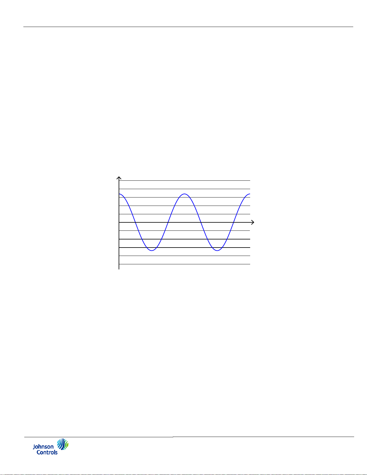
ballasts make current demands that do not match the sinusoidal waveform of AC
electricity. As a result, the current waveform feeding these loads is periodic but not
sinusoidal. Figure 1.10 shows a normal, sinusoidal current waveform. This example
has no distortion.

1: Three-Phase Power Measurement

Figure 1.10: Nondistorted Current Waveform

Figure 1.11 shows a current waveform with a slight amount of harmonic distortion.
The waveform is still periodic and is fluctuating at the normal 60 Hz frequency.
However, the waveform is not a smooth sinusoidal form as seen in Figure 1.10.

EM-4000 Series Meters Installation and Operation Manual 1-14

1: Three-Phase Power Measurement

–1000

–500

0

500

1000

t

)spma( tnerruC

a

2a

–1500

1500

Time

Amps

3rd harmonic

5th harmonic

7th harmonic

Total

fundamental

– 500

0

500

1000

Figure 1.11: Distorted Current Waveform

The distortion observed in Figure 1.11 can be modeled as the sum of several sinusoi­dal waveforms of frequencies that are multiples of the fundamental 60 Hz frequency.
This modeling is performed by mathematically disassembling the distorted waveform
into a collection of higher frequency waveforms.

These higher frequency waveforms are referred to as harmonics. Figure 1.12 shows
the content of the harmonic frequencies that make up the distortion portion of the
waveform in Figure 1.11.

Figure 1.12: Waveforms of the Harmonics

EM-4000 Series Meters Installation and Operation Manual 1-15

1: Three-Phase Power Measurement

The waveforms shown in Figure 1.12 are not smoothed but do provide an indication of
the impact of combining multiple harmonic frequencies together.

When harmonics are present it is important to remember that these quantities are
operating at higher frequencies. Therefore, they do not always respond in the same
manner as 60 Hz values.

Inductive and capacitive impedance are present in all power systems. We are accus­tomed to thinking about these impedances as they perform at 60 Hz. However, these
impedances are subject to frequency variation.

X

= jL and

L

= 1/jC

X

C

At 60 Hz,  = 377; but at 300 Hz (5th harmonic)  = 1,885. As frequency changes
impedance changes and system impedance characteristics that are normal at 60 Hz
may behave entirely differently in the presence of higher order harmonic waveforms.

Traditionally, the most common harmonics have been the low order, odd frequencies,
such as the 3rd, 5th, 7th, and 9th. However newer, non-linear loads are introducing
significant quantities of higher order harmonics.

Since much voltage monitoring and almost all current monitoring is performed using
instrument transformers, the higher order harmonics are often not visible. Instrument
transformers are designed to pass 60 Hz quantities with high accuracy. These devices,
when designed for accuracy at low frequency, do not pass high frequencies with high
accuracy; at frequencies above about 1200 Hz they pass almost no information. So
when instrument transformers are used, they effectively filter out higher frequency
harmonic distortion making it impossible to see.

However, when monitors can be connected directly to the measured circuit (such as
direct connection to a 480 volt bus) the user may often see higher order harmonic
distortion. An important rule in any harmonics study is to evaluate the type of equip­ment and connections before drawing a conclusion. Not being able to see harmonic
distortion is not the same as not having harmonic distortion.

It is common in advanced meters to perform a function commonly referred to as
waveform capture. Waveform capture is the ability of a meter to capture a present
picture of the voltage or current waveform for viewing and harmonic analysis.

EM-4000 Series Meters Installation and Operation Manual 1-16

Typically a waveform capture will be one or two cycles in duration and can be viewed
as the actual waveform, as a spectral view of the harmonic content, or a tabular view
showing the magnitude and phase shift of each harmonic value. Data collected with
waveform capture is typically not saved to memory. Waveform capture is a real-time
data collection event.

Waveform capture should not be confused with waveform recording that is used to
record multiple cycles of all voltage and current waveforms in response to a transient
condition.

1.5: Power Quality

Power quality can mean several different things. The terms "power quality" and
"power quality problem" have been applied to all types of conditions. A simple defini­tion of "power quality problem" is any voltage, current or frequency deviation that

1: Three-Phase Power Measurement

results in mis-operation or failure of customer equipment or systems. The causes of
power quality problems vary widely and may originate in the customer equipment, in
an adjacent customer facility or with the utility.

In his book Power Quality Primer, Barry Kennedy provided information on different
types of power quality problems. Some of that information is summarized in Table

1.3.

EM-4000 Series Meters Installation and Operation Manual 1-17

1: Three-Phase Power Measurement

Cause Disturbance Type Source

Impulse transient Transient voltage disturbance,

sub-cycle duration

Oscillatory
transient with decay

Transient voltage, sub-cycle
duration

Sag/swell RMS voltage, multiple cycle

duration

Interruptions RMS voltage, multiple

seconds or longer duration

Under voltage/over voltage RMS voltage, steady state,

multiple seconds or longer
duration

Voltage flicker RMS voltage, steady state,

repetitive condition

Harmonic distortion Steady state current or volt-

age, long-term duration

Lightning
Electrostatic discharge
Load switching
Capacitor switching

Line/cable switching
Capacitor switching
Load switching

Remote system faults

System protection
Circuit breakers
Fuses
Maintenance

Motor starting
Load variations
Load dropping

Intermittent loads
Motor starting
Arc furnaces

Non-linear loads
System resonance

Table 1.3: Typical Power Quality Problems and Sources

It is often assumed that power quality problems originate with the utility. While it is
true that many power quality problems can originate with the utility system, many
problems originate with customer equipment. Customer-caused problems may mani­fest themselves inside the customer location or they may be transported by the utility
system to another adjacent customer. Often, equipment that is sensitive to power
quality problems may in fact also be the cause of the problem.

If a power quality problem is suspected, it is generally wise to consult a power quality
professional for assistance in defining the cause and possible solutions to the
problem.

EM-4000 Series Meters Installation and Operation Manual 1-18

2: Meter Overview and Specifications

2: Meter Overview and Specifications

2.1: EM-4000 Meter Overview

The EM-4000 meter is a multifunction, data
logging, power and energy meter with wave­form recording capability, designed to be
used in electrical substations, panel boards,
as a power meter for OEM equipment, and as
a primary revenue meter, due to its high per­formance measurement capability. The unit
provides multifunction measurement of all
electrical parameters and makes the data
available in multiple formats via display and
communication systems. The unit also has
data logging and load profiling to provide
historical data analysis.

The EM-4000 meter offers 2 MegaBytes of Flash memory. (Because the memory is
flash-based rather than NVRAM (non-volatile random-access memory), some sectors
are reserved for overhead, erase procedures, and spare sectors for long-term wear
reduction.) The unit provides you with up to four logs: three historical logs and a
sequence of events log.

The purposes of these features include historical load profiling, voltage analysis, and
recording power factor distribution. The EM-4000 meter’s real-time clock allows all
events to be time stamped.

The EM-4000 meter is designed with advanced measurement capabilities, allowing it
to achieve high performance accuracy. It is specified as a 0.2% class energy meter for
billing applications as well as a highly accurate panel indication meter. It supplies

0.001 Hz Frequency measurement which meets generating stations’ requirements.

The EM-4000 meter provides additional capabilities, including standard RS485,

Figure 2.1: EM-4000 meter

Modbus® protocol support, and an IrDA port for remote interrogation.

Features of the EM-4000 meter include:

• 0.2% Class revenue certifiable energy and demand metering

• Meets ANSI C12.20 (0.2%) and IEC 62053-22 (0.2%) classes

EM-4000 Series Meters Installation and Operation Manual

2-1

2: Meter Overview and Specifications

• Multifunction measurement including voltage, current, power, frequency, energy,

etc.

• Optional secondary Voltage display (see the EM Series Communicator Software

User Manual for instructions on setting up this feature)

• Percentage of Load bar for analog meter reading

• 0.001% Frequency measurement for Generating stations

• Interval energy logging

• Line frequency time synchronization

• Easy to use faceplate programming

• IrDA port for laptop PC remote read

• RS485 communication

• Transformer/Line Loss compensation (see the EM Series Communicator Software

User Manual for instructions on using this feature)

• CT/PT compensation (see the EM Series Communicator Software

instructions on using this feature)

2.1.1: Voltage and Current Inputs

Universal Voltage Inputs

Voltage inputs allow measurement up to Nominal 576VAC (Phase to Reference) and
721VAC (Phase to Phase). This insures proper meter safety when wiring directly to
high Voltage systems. The unit will perform to specification on 69 Volt, 120 Volt, 230
Volt, 277 Volt, and 347 Volt power systems.

NOTE: Higher Voltages require the use of potential transformers (PTs).

User Manual for

Current Inputs

The unit supports a 5 Amp secondary for current measurements.

The current inputs are only to be connected to external current transformers.

EM-4000 Series Meters Installation and Operation Manual

2-2

2: Meter Overview and Specifications

The EM-4000 Series meter’s current inputs use a unique dual input method:

Method 1: CT Pass Through:

The CT wire passes directly through the meter without any physical termination on
the meter. This insures that the meter cannot be a point of failure on the CT circuit.
This is preferable for utility users when sharing relay class CTs. No Burden is added to
the secondary CT circuit.

Method 2: Current “Gills”:

This unit additionally provides ultra-rugged termination pass through bars that allow
CT leads to be terminated on the meter. This, too, eliminates any possible point of
failure at the meter. This is a preferred technique for insuring that relay class CT
integrity is not compromised (the CT will not open in a fault condition).

2.1.2: Ordering Information

EM-4000 Series Meter Ordering chart

Product-

Series

EM-4
EM-4000
Series
Meter

Example:

EM-4460-05-AI00
which translates to an EM-4000 Series meter with Modbus® communication, 60Hz
system, 90-265VAC/100-370VDC Power Supply, 5A Secondary Class, and ANSI

Network

Protocol Freq.

4
Modbus

50
50 H z
System

60
60 Hz
System

-Power
Supply

-0
90-265
VAC/
100-370
VDC

DI

Current

Class

5
5 Amp
S e c o n d a r y

Mounting 0 0

AI
ANSI
Mounting

DIN
Mounting

-

mounting. The last two options do not pertain to the EM-4000 Series meter, so the
ordering code contains 0s for them.

EM-4000 Series Meters Installation and Operation Manual

2-3

2: Meter Overview and Specifications

CodeNumber Description

UNICOM2500 RS485toRS232Converter
UNICOM2500ͲF RS485toRS232orFiberConverter
E145350 2wireto4wireRS485cable,6'longforusewithUnicom2500/2500F
EIͲ1SPͲ100Ͳ00 100/5AsplitcoreCTwith.84"x2.0"window
EIͲ1SPͲ200Ͳ00 200/5AsplitcoreCTwith.84"x2.0"window
EIͲWC4Ͳ400ͲRA05

400/5AsplitcoreCTwith1.3"x1.7"window
EIͲ615Ͳ401 400/5AsplitcoreCTwith1.3"x1.6"window
EIͲ3SPͲ600Ͳ00 600/5AsplitcoreCTwith2.19"x3.25"window
EIͲ3SPͲ800Ͳ00 800/5AsplitcoreCTwith2.19"x3.25"window
EIͲ5SPͲ1200Ͳ00 1200/5AsplitcoreCTwith2.88"x4.25"window
EIͲ7SPͲ1600Ͳ00

1600/5AsplitcoreCTwith2.88"x6.25"window
EIͲ91SPͲ2000Ͳ00 2000/5AsplitcoreCTwith4.00"x7.50"window
EIͲ91SPͲ3000Ͳ00 3000/5AsplitcoreCTwith4.00"x7.50"window
EIͲ91SPͲ4000Ͳ00 4000/5AsplitcoreCTwith4.00"x7.50"window
EIͲ2SFTͲ500

50/5AsolidcoreCTwith1.13'IDwithterminalsandfeet
EIͲ2SFTͲ101 100/5AsolidcoreCTwith1.13'IDwithterminalsandfeet
EIͲ2SFTͲ201 200/5AsolidcoreCTwith1.13'IDwithterminalsandfeet
EIͲ5SFTͲ401 400/5AsolidcoreCTwith1.56'IDwithterminalsandfeet
EIͲ2DARLͲ500

50/5AsolidcoreCTwith1.00'ID
EIͲ2DARLͲ101 100/5AsolidcoreCTwith1.00'ID
EIͲ2DARLͲ201 200/5AsolidcoreCTwith1.00'ID
EIͲ5ARLͲ401 400/5AsolidcoreCTwith1.56'IDwithterminalsandfeet
EIͲ7RLͲ601 600/5AsolidcoreCTwith2.50'ID
EIͲ7RLͲ801 800/5AsolidcoreCTwith2.50'ID
EIͲ76RLͲ122

1200/5AsolidcoreCTwith3.00'ID
EIͲ8RLͲ162 1600/5AsolidcoreCTwith3.00'ID
EIͲ2VTͲ460Ͳ480FF 3PhDeltaͲDelta480/120VPotentialTransformer,fusedP&S
EIͲ3VT472Ͳ480Ͳ208FF 3PhWyeͲWye277/480:208/120VPT,fusedP&S
EIͲ75481P 480/120,75VAcontrolpowertransforme

r

EIͲCP protectivefuse/fuseblockki

t

EIͲMSB10Ͳ400 surgeprotecto

r

EIͲSBͲ6TC EMSeriesMetersixpoleCTshortingblockwithprotectivecove

r

EIͲFPͲ8110SAͲ25 EMSeriesMeterfibercom10/100CoppertoFibermediaconverte

r

CAB6490 EMSeriesMeterUSBtoIrDAadapter
ANT18769 remotewirelessantennaki

t

The following chart lists components that can be ordered along with the EM-4000
meter.

EM-4000 Series Meters Installation and Operation Manual

2-4

2: Meter Overview and Specifications

2.1.4: Measured Values

The EM-4000 Series meter provides the following measured values all in real time
instantaneous. As the table below shows, some values are also available in average,
maximum and minimum.

Table 1:

Measured Values Instantaneous Avg Max Min

Voltage L-N X X X

Voltage L-L X X X

Current per Phase X X X X

Current Neutral X X X X

WATT(A,B,C,Tot.) X X X X

VAR (A,B,C,Tot.) X X X X

VA (A,B,C,Tot.) X X X X

PF (A,B,C,Tot.) X X X X

+Watt-Hour (A,B,C,Tot.) X

-Watt-Hour (A,B,C,Tot.) X

Watt-Hour Net X

+VAR-Hour (A,B,C,Tot.) X

-VAR-Hour (A,B,C,Tot.) X

VAR-Hour Net (A,B,C,Tot.) X

VA-Hour (A,B,C,Tot.) X

Frequency X X X

Voltage Angles X

Current Angles X

% of Load Bar X

Waveform Scope X

EM-4000 Series Meters Installation and Operation Manual

2-5

2.1.5: Utility Peak Demand

The EM-4000 Series meter provides user-configured Block (Fixed) window or Rolling
window Demand modes. This feature lets the user set up a customized Demand pro­file. Block window Demand mode records the average demand for time intervals the
user defines (usually 5, 15 or 30 minutes). Rolling window Demand mode functions
like multiple, overlapping Block windows. The user defines the subintervals at which
an average of Demand is calculated. An example of Rolling window Demand mode
would be a 15-minute Demand block using 5-minute subintervals, thus providing a
new Demand reading every 5 minutes, based on the last 15 minutes.

Utility Demand features can be used to calculate Watt, VAR, VA and PF readings.
Voltage provides an instantaneous Max and Min reading which displays the highest
surge and lowest sag seen by the meter. All other parameters offer Max and Min
capability over the user-selectable averaging period.

2: Meter Overview and Specifications

EM-4000 Series Meters Installation and Operation Manual

2-6

2.2: Specifications

Power Supply

Range: Universal, (90 to 265)

Power Consumption: (5 to 10)VA, (3.5 to 7)W -

Voltage Inputs

(For Accuracy specifications, see Section 2.4.)

2: Meter Overview and Specifications

VAC @50/60Hz or (100 to 370)VDC

depending on the meter’s hardware

configuration

Absolute Maximum Range: Universal, Auto-ranging:

Phase to Reference (Va, Vb, Vc to

Vref): (20 to 576)VAC

Phase to Phase (Va to Vb, Vb to Vc,

Vc to Va): (0 to 721)VAC

Supported hookups: 3 Element Wye, 2.5 Element Wye,

2 Element Delta, 4 Wire Delta

Input Impedance: 1M Ohm/Phase

Burden: 0.36VA/Phase Max at 600 Volts;

0.014VA at 120 Volts

Pickup Voltage: 20VAC

Connection: 7 Pin 0.400” Pluggable Terminal

Block

AWG#12 -26/ (0.129 -3.31) mm

EM-4000 Series Meters Installation and Operation Manual

2-7

2

2: Meter Overview and Specifications

Fault Withstand: Meets IEEE C37.90.1

Reading: Programmable Full Scale to any PT

ratio

Current Inputs

(For Accuracy specifications, see Section 2.4.)

Class 10: 5A Nominal, 10A Maximum

Burden: 0.005VA Per Phase Max at 11 Amps

Pickup Current: 0.1% of Nominal (0.2% of Nominal

if using Current Only mode, that is,

there is no connection to the

Voltage inputs)

Connections: O Lug or U Lug electrical connec-

tion (Figure 4.1)

Pass through wire, 0.177” / 4.5mm

maximum diameter (Figure 4.2)

Quick connect, 0.25” male tab

(Figure 4.3)

Fault Withstand (at 23

Reading: Programmable Full Scale to any CT

o

C): 100A/10sec., 300A/3sec.,

500A/1sec.

ratio

Continuous Current Withstand: 20 Amps for screw terminated or

pass through connections

EM-4000 Series Meters Installation and Operation Manual

2-8

2: Meter Overview and Specifications

KYZ/RS485 Port Specifications

RS485 Transceiver; meets or exceeds EIA/TIA-485 Standard

Type: Two-wire, half duplex

Min. input Impedance: 96kΩ

Max. output current: ±60mA

Wh Pulse

KYZ output contacts, and infrared LED light pulses through face plate (see Section 6.4
for Kh values):

Pulse Width: 90ms

Full Scale Frequency: ~3Hz

Contact type: Solid state – SPDT (NO – C – NC)

Relay type: Solid state

Peak switching voltage: DC ±350V

Continuous load current: 120mA

Peak load current: 350mA for 10ms

On resistance, max.: 35Ω

Leakage current: 1µA@350V

Isolation: AC 3750V

Reset state: (NC - C) Closed; (NO - C) Open

EM-4000 Series Meters Installation and Operation Manual

2-9

2: Meter Overview and Specifications

(De-energized state)

N

O

C

N

C

90ms 90ms

][

3600

][

WattP

pulse

Watthour

Kh

sT

»
¼

º

«
¬

ª



LED

ON

LED

ON

LED
OFF

LED
OFF

LED

OFF

IR LED Light Pulses

Through face plate

N

O

C

N

C

N

O

C

N

C

N

O

C

N

C

N

O

C

N

C

N

O

C

N

C

KYZ output

Contact States

Through Backplate

P

[Watt] - Not a scaled value

K

h  See Section 6-4 for values

Infrared LED:

Peak Spectral wavelength: 940nm

Reset state: Off

Internal schematic:

Output timing:

EM-4000 Series Meters Installation and Operation Manual

2-10

Isolation

Environmental Rating

2: Meter Overview and Specifications

All Inputs and Outputs are galvani­cally isolated to 2500 VAC

Storage: (-20 to +70)

Operating: (-20 to +70)

o

C

o

C

Humidity: to 95% RH Non-condensing

Faceplate Rating: NEMA12 (Water Resistant), mount-

ing gasket included

Measurement Methods

Voltage, current: True RMS

Power: Sampling at over 400 samples per

cycle on all channels

Update Rate

Watts, VAR and VA: Every 6 cycles (e.g., 100ms @ 60

Hz)

All other parameters: Every 60 cycles (e.g., 1 s @ 60 Hz)

1 second for Current Only measure­ment, if reference Voltage is not
available

Communication

Standard:

1. RS485 port through backplate

2. IrDA port through faceplate

3. Energy pulse output through backplate and Infrared LED through faceplate

EM-4000 Series Meters Installation and Operation Manual

2-11

2: Meter Overview and Specifications

Protocols: Modbus® RTU, Modbus® ASCII,
DNP 3.0

Com Port Baud Rate: RS485 Only: 1200, 2400, 4800;

All Com Ports: 9600 to 57600 bps

Com Port Address: 001-247

Data Format: 8 Bit, No Parity (RS485: also Even

or Odd Parity)

Mechanical Parameters

Dimensions: see Chapter 3.

Weight: 2 pounds/ 0.9kg (ships in a 6”

/15.24cm cube container)

2.3: Compliance

• UL/cUL Listed

• CE (EN61326-1, FCC Part 15, Subpart B, Class A)

• IEC 62053-22 (0.2% Class)

• ANSI C12.20 (0.2% Accuracy)

• ANSI (IEEE) C37.90.1 Surge Withstand

• ANSI C62.41 (Burst)

• EN61000-6-2 Immunity for Industrial Environments: 2005

• EN61000-6-4 Emission Standards for Industrial Environments: 2007

• EN61326 EMC Requirements: 2006

EM-4000 Series Meters Installation and Operation Manual

2-12

2.4: Accuracy

(For full Range specifications see Section 2.2.)

2: Meter Overview and Specifications

EM-4000 Clock Accuracy: Max. +/-2 seconds per day at 25

For 23

o

C, 3 Phase balanced Wye or Delta load, at 50 or 60 Hz (as per order), 5A

(Class 10) nominal unit, accuracy as follows:

Table 2:

Parameter Accuracy Accuracy Input Range1

Voltage L-N [V] 0.1% of reading (69 to 480)V

Voltage L-L [V]

Current Phase [A]

Current Neutral (calcu­lated) [A]

Active Power Total [W]

Active Energy Total [Wh]

0.2% of reading

0.1% of reading

2% of Full Scale

0.2% of reading

0.2% of reading

2

1, 3

1

1, 2

1, 2

(120 to 600)V

(0.15 to 5) A

(0.15 to 5) A @ (45 to 65)
Hz

(0.15 to 5) A @ (69 to

480) V @ +/- (0.5 to 1)
lag/lead PF

(0.15 to 5) A @ (69 to

480) V @ +/- (0.5 to 1)
lag/lead PF

o

C

Reactive Power Total
[VAR]

0.2% of reading

1, 2

(0.15 to 5) A @ (69 to

480) V @ +/- (0 to 0.8)
lag/lead PF

Reactive Energy Total
[VARh]

0.2% of reading

1, 2

(0.15 to 5) A @ (69 to

480) V @ +/- (0 to 0.8)
lag/lead PF

Apparent Power Total [VA]

0.2% of reading

1, 2

(0.15 to 5) A @ (69 to

480) V @ +/- (0.5 to 1)
lag/lead PF

Apparent Energy Total
[VAh]

0.2% of reading

1, 2

(0.15 to 5) A @ (69 to

480) V @ +/- (0.5 to 1)
lag/lead PF

Power Factor

0.2% of reading

1, 2

(0.15 to 5) A @ (69 to

480) V @ +/- (0.5 to 1)
lag/lead PF

Frequency [Hz] +/- 0.001 Hz (45 to 65) Hz

Load Bar

+/- 1 segment

1

(0.005 to 6) A

EM-4000 Series Meters Installation and Operation Manual

2-13

2: Meter Overview and Specifications

1

• For 2.5 element programmed units, degrade accuracy by an additional 0.5% of
reading.

• For 1A (Class 2) Nominal, degrade accuracy to 0.5% of reading for watts and

energy; all other values 2 times rated accuracy.

• For 1A (Class 2) Nominal, the input current range for accuracy specification is
20% of the values listed in the table.

2

For unbalanced Voltage inputs where at least one crosses the 150V auto-scale

threshold (for example, 120V/120V/208V system), degrade the accuracy to 0.4%
of reading.

3

With reference Voltage applied (VA, VB, or VC). Otherwise, degrade accuracy to

0.2%. See hookup diagrams 8, 9, and 10 in Chapter 4.

EM-4000 Series Meters Installation and Operation Manual

2-14

3: Mechanical Installation

0.06 [

0.15]

0.77 [1.95]

5.02 [12

.75]

Gasket

3.25 [8.26]

4.85 [12.32]

4.85 [12

.32]

0.95 [2.41]

3.1: Introduction

The EM-4000 meter can be installed using a standard ANSI C39.1 (4” round) or an
IEC 92mm DIN (square) form. In new installations, simply use existing DIN or ANSI
punches. For existing panels, pull out old analog meters and replace them with the
EM-4000 meter. See Chapter 4 for wiring diagrams.

NOTE: The drawings shown below and on the next page give you the meter dimen­sions in inches and centimeters [cm shown in brackets]. Tolerance is +/- 0.1” [.25
cm].

3: Mechanical Installation

Figure 3.1: Meter Front and Side Dimensions

EM-4000 Series Meters Installation and Operation Manual

3-1

3: Mechanical Installation

3.56 [9.04]

3.56 [9.04]

CM



CM

3Q

8v

v

Figure 3.2: Meter Back Dimensions

Figure 3.3: ANSI and DIN Cutout Dimensions

Recommended Tools for EM-4000 meter Installation:

• #2 Phillips screwdriver

• Small adjustable wrench

• Wire cutters

The EM-4000 meter is designed to withstand harsh environmental conditions; how­ever it is recommended you install it in a dry location, free from dirt and corrosive
substances (see Environmental specifications in Chapter 2).

EM-4000 Series Meters Installation and Operation Manual

3-2

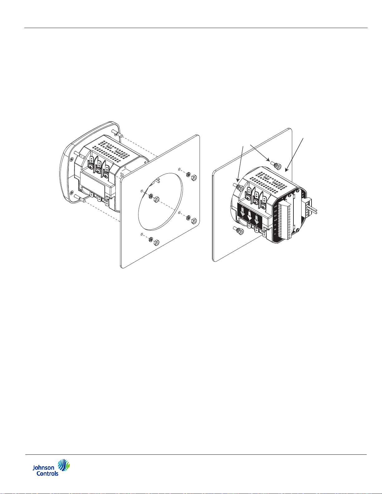
3.2: ANSI Installation Steps

ANSI Installation

ANSI Studs

4.0” Round form

1. Slide meter with Mounting Gasket into panel.

2. Secure from back of panel with flat washer, lock washer and nut on each threaded
rod. Use a small wrench to tighten. Do not overtighten. The maximum installation
torque is 0.4 Newton-Meter.

3: Mechanical Installation

Figure 3.4: ANSI Installation

EM-4000 Series Meters Installation and Operation Manual

3-3

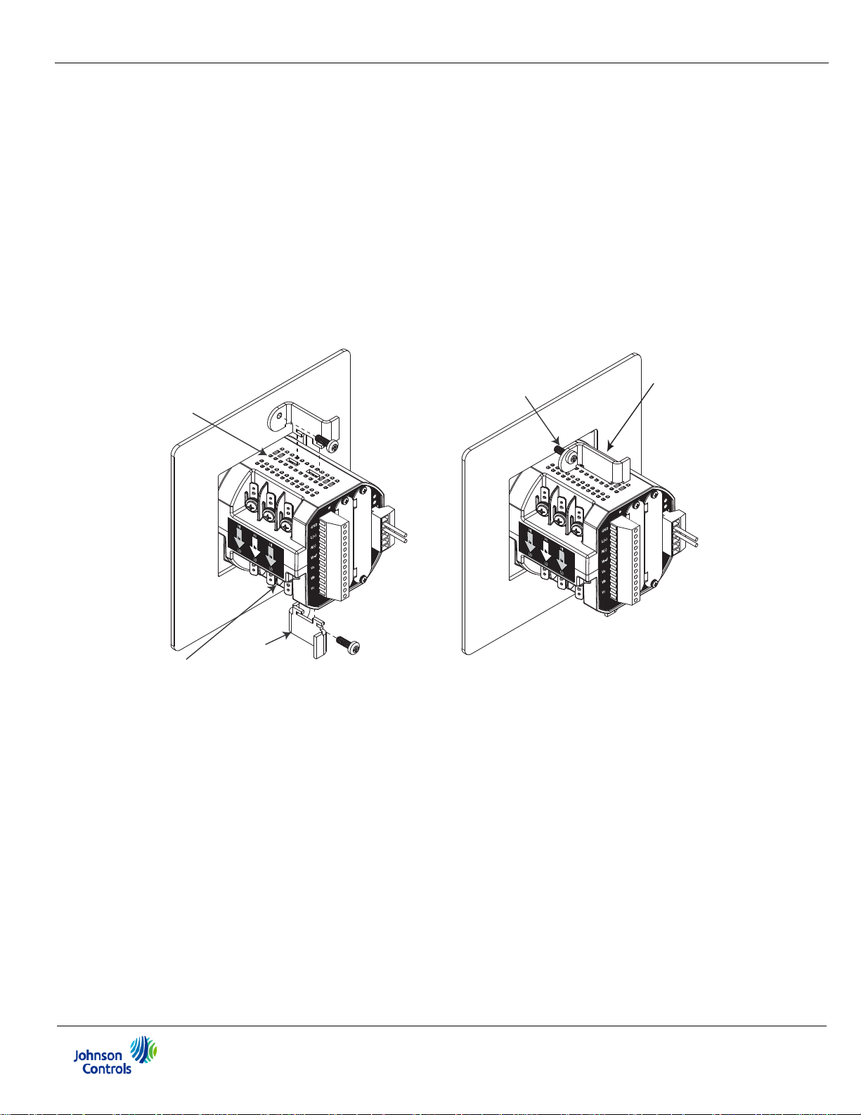
3.3: DIN Installation Steps

DIN mounting
bracket

Top mounting
bracket groove

Bottom
mounting
bracket groove

DIN Mounting brackets

Remove (unscrew) ANSI studs
for DIN installation

DIN Installation

92mm Square
form

1. Slide meter with NEMA 12 Mounting Gasket into panel (remove ANSI Studs, if in
place).

2. From back of panel, slide 2 DIN Mounting Brackets into grooves in top and bottom
of meter housing. Snap into place.

3. Secure meter to panel by using a #2 Phillips screwdriver to tighten the screw on
each of the two mounting brackets. Do not overtighten: the maximum installation
torque is 0.4 Newton-Meter.

3: Mechanical Installation

Figure 3.5: DIN Installation

EM-4000 Series Meters Installation and Operation Manual

3-4

4: Electrical Installation

4: Electrical Installation

4.1: Considerations When Installing Meters

Installation of the EM-4000 meter must be performed only by quali­fied personnel who follow standard safety precautions during all pro­cedures. Those personnel should have appropriate training and
experience with high Voltage devices. Appropriate safety gloves,
safety glasses and protective clothing are recommended.

During normal operation of the EM-4000 meter, dangerous Voltages flow through
many parts of the meter, including: Terminals and any connected CTs (Current Trans­formers) and PTs (Potential Transformers), all I/O Modules (Inputs and Outputs) and
their circuits.

All Primary and Secondary circuits can, at times, produce lethal Voltages and
currents. Avoid contact with any current-carrying surfaces.

Do not use the meter or any I/O Output device for primary protection or in
an energy-limiting capacity. The meter can only be used as secondary
protection.

Do not use the meter for applications where failure of the meter may cause harm or
death.

Do not use the meter for any application where there may be a risk of fire.

All meter terminals should be inaccessible after installation.

Do not apply more than the maximum Voltage the meter or any attached device can
withstand. Refer to meter and/or device labels and to the specifications for all devices
before applying voltages. Do not HIPOT/Dielectric test any Outputs, Inputs or Com­munications terminals.

Caution: Risk of Property Damage.

Do not apply power to the system before checking all wiring connec­tions. Short circuited or improperly connected wires may result in
permanent damage to the equipment.

EM-4000 Series Meters Installation and Operation Manual

4-1

4: Electrical Installation

Johnson Controls recommends the use of Fuses for Voltage leads and power supply
and shorting blocks to prevent hazardous Voltage conditions or damage to CTs, if the
meter needs to be removed from service. CT grounding is optional, but recom­mended.

NOTE: The current inputs are only to be connected to external current transformers
provided by the installer. The CTs shall be Approved or Certified and rated for the
current of the meter used.

Caution: Risk of Property Damage.

Ensure that the power source conforms to the requirements of the
equipment. Failure to use a correct power source may result in per­manent damage to the equipment.

L'installation des compteurs de EM-4000 Series doit être effectuée
seulement par un personnel qualifié qui suit les normes relatives aux
précautions de sécurité pendant toute la procédure. Le personnel
doit avoir la formation appropriée et l'expérience avec les appareils
de haute tension. Des gants de sécurité, des verres et des vête-

ments de protection appropriés sont recommandés.

AVERTISSEMENT! Pendant le fonctionnement normal du compteur EM-4000 Series
des tensions dangereuses suivant de nombreuses pièces, notamment, les bornes et
tous les transformateurs de courant branchés, les transformateurs de tension, toutes
les sorties, les entrées et leurs circuits. Tous les circuits secondaires et primaires

peuvent parfois produire des tensions de létal et des courants. Évitez le con­tact avec les surfaces sous tensions. Avant de faire un travail dans le compt­eur, assurez-vous d'éteindre l'alimentation et de mettre tous les circuits
branchés hors tension.

Ne pas utiliser les compteurs ou sorties d'appareil pour une protection pri­maire ou capacité de limite d'énergie. Le compteur peut seulement être
utilisé comme une protection secondaire.

Ne pas utiliser le compteur pour application dans laquelle une panne de compteur
peut causer la mort ou des blessures graves.

Ne pas utiliser le compteur ou pour toute application dans laquelle un risque
d'incendie est susceptible.

EM-4000 Series Meters Installation and Operation Manual

4-2

4: Electrical Installation

Toutes les bornes de compteur doivent être inaccessibles après l'installation.

Ne pas appliquer plus que la tension maximale que le compteur ou appareil relatif
peut résister. Référez-vous au compteur ou aux étiquettes de l'appareil et les spécifi­cations de tous les appareils avant d'appliquer les tensions. Ne pas faire de test
HIPOT/diélectrique, une sortie, une entrée ou un terminal de réseau.

Les entrées actuelles doivent seulement être branchées aux transformateurs externes
actuels.

Johnson Controls recommande d'utiliser les fusibles pour les fils de tension et alimen­tations électriques, ainsi que des coupe-circuits pour prévenir les tensions dangere­uses ou endommagements de transformateur de courant si l'unité EM-4000 Series
doit être enlevée du service. Un côté du transformateur de courant doit être mis à
terre.

NOTE: Les entrées actuelles doivent seulement être branchées dans le transforma­teur externe actuel par l'installateur. Le transformateur de courant doit être approuvé
ou certifié et déterminé pour le compteur actuel utilisé.

IMPORTANT!

IF THE EQUIPMENT IS USED IN A MANNER NOT SPECIFIED
BY THE MANUFACTURER, THE PROTECT I ON PROVIDED BY
THE EQUIPMENT MAY BE IMPAIRED.

• THERE IS NO REQUIRED PREVENTIVE MAINTENANCE OR INSPEC­ TION NECESSARY FOR SAFETY. HOWEVER, ANY REPAIR OR MAIN­ TENANCE SHOULD BE PERFORMED BY THE FACTORY.

DISCONNECT DEVICE: The following part is considered the equip­ment disconnect device. A SWITCH OR CIRCUIT-BREAKER SHALL BE
INCLUDED IN THE END-USE EQUIPMENT OR BUILDING INSTALLA­TION. THE SWITCH SHALL BE IN CLOSE PROXIMITY TO THE EQUIP­MENT AND WITHIN EASY REACH OF THE OPERATOR. THE SWITCH
SHALL BE MARKED AS THE DISCONNECTING DEVICE FOR THE
EQUIPMENT.

EM-4000 Series Meters Installation and Operation Manual

4-3

4: Electrical Installation

IMPORTANT! SI L'ÉQUIPEMENT EST UTILISÉ D'UNE FAÇON
NON SPÉCIFIÉE PAR LE FABRICANT, LA PROTECTION FOUR­NIE PAR L'ÉQUIPEMENT PEUT ÊTRE ENDOMMAGÉE.

NOTE: Il N'Y A AUCUNE MAINTENANCE REQUISE POUR LA PRÉVENTION OU INSPEC-

TION NÉCESSAIRE POUR LA SÉCURITÉ. CEPENDANT, TOUTE RÉPARATION OU MAIN­TENANCE DEVRAIT ÊTRE RÉALISÉE PAR LE FABRICANT.

DÉBRANCHEMENT DE L'APPAREIL : la partie suivante est con­sidérée l'appareil de débranchement de l'équipement.

UN INTERRUPTEUR OU UN DISJONCTEUR DEVRAIT ÊTRE INCLUS
DANS L'UTILISATION FINALE DE L'ÉQUIPEMENT OU L'INSTALLATION.

L'INTERRUPTEUR DOIT ÊTRE DANS UNE PROXIMITÉ PROCHE DE
L'ÉQUIPEMENT ET A LA PORTÉE DE L'OPÉRATEUR. L'INTERRUPTEUR DOIT AVOIR LA
MENTION DÉBRANCHEMENT DE L'APPAREIL POUR L'ÉQUIPEMENT.

4.2: CT Leads Terminated to Meter

The EM-4000 meter is designed to have current inputs wired in one of three ways.
Figure 4.1 shows the most typical connection where CT Leads are terminated to the
meter at the current gills. This connection uses nickel-plated brass studs (current
gills) with screws at each end. This connection allows the CT wires to be terminated
using either an “O” or a “U” lug. Tighten the screws with a #2 Phillips screwdriver. The
maximum installation torque is 0.7376 foot-pounds (1 Newton-Meter).

EM-4000 Series Meters Installation and Operation Manual

4-4

4: Electrical Installation

Current Gills
(nickel-plated
brass studs)

Other current connections are shown in figures 4.2 and 4.3. Voltage and RS485/KYZ
connections are shown in Figure 4.4.

Figure 4.1: CT Leads Terminated to Meter, #8 Screw for Lug Connection

Wiring Diagrams are shown in Section 4.8 of this chapter.

Communications connections are detailed in Chapter 5.

EM-4000 Series Meters Installation and Operation Manual

4-5

4: Electrical Installation

$5XJSFQBTTJOH
UISPVHINFUFS

$VSSFOUHJMMT
SFNPWFE

4.3: CT Leads Pass Through (No Meter Termination)

The second method allows the CT wires to pass through the CT inputs without termi­nating at the meter. In this case, remove the current gills and place the CT wire
directly through the CT opening. The opening accommodates up to 0.177” / 4.5mm
maximum diameter CT wire.

Figure 4.2: Pass Through Wire Electrical Connection

EM-4000 Series Meters Installation and Operation Manual

4-6

4.4: Quick Connect Crimp-on Terminations

Quick connect
crimp-on
terminations

For quick termination or for portable applications, 0.25” quick connect crimp-on
connectors can also be used

4: Electrical Installation

Figure 4.3: Quick Connect Electrical Connection

EM-4000 Series Meters Installation and Operation Manual

4-7

4: Electrical Installation

QPXFS

TVQQMZ
JOQVUT

7PMUBHF
JOQVUT

34PVUQVU
%0/05QVU
7PMUBHFPO
UIFTF
UFSNJOBMT

,:;

*

4.5: Voltage and Power Supply Connections

Voltage inputs are connected to the back of the unit via optional wire connectors. The

connectors accommodate AWG# 12 -26/ (0.129 - 3.31)mm

2

.

*The power supply voltage range is Universal, (90 to 265) VAC @50/60Hz or

(100 to 370)VDC.

4.6: Ground Connections

The meter’s Ground terminals should be connected directly to the installation’s

protective earth ground. Use AWG# 12/2.5 mm

WARNING: Risk of Electric Shock.
Ground the meter according to local, national, and regional regulations.
Failure to ground the meter may result in electric shock and severe
personal injury or death.

AVERTISSEMENT: Risque de décharge électrique.

Effectuer la mise à terre selon les règlements locaux, nationaux et régionaux. La non mise
à la terre du compteur peut provoquer une décharge électrique, des blessures graves ou
provoquer la mort.

Figure 4.4: Meter Connections

2

wire for this connection.

EM-4000 Series Meters Installation and Operation Manual

4-8

4.7: Voltage Fuses

Johnson Controls recommends the use of fuses on each of the sense voltages and on
the control power.

• Use a 0.1 Amp fuse on each voltage input.

• Use a 3 Amp Slow Blow fuse on the power supply.

4: Electrical Installation

EM-4000 Series Meters Installation and Operation Manual

4-9

4.8: Electrical Connection Diagrams

The following pages contain electrical connection diagrams for the EM-4000 meter.
Choose the diagram that best suits your application. Be sure to maintain the CT
polarity when wiring.

The diagrams are presented in the following order:

1. Three Phase, Four-Wire System Wye/Delta with Direct Voltage, 3 Element

a. Example of Dual-Phase Hookup

b. Example of Single Phase Hookup

2. Three Phase, Four-Wire System Wye with Direct Voltage, 2.5 Element

4: Electrical Installation

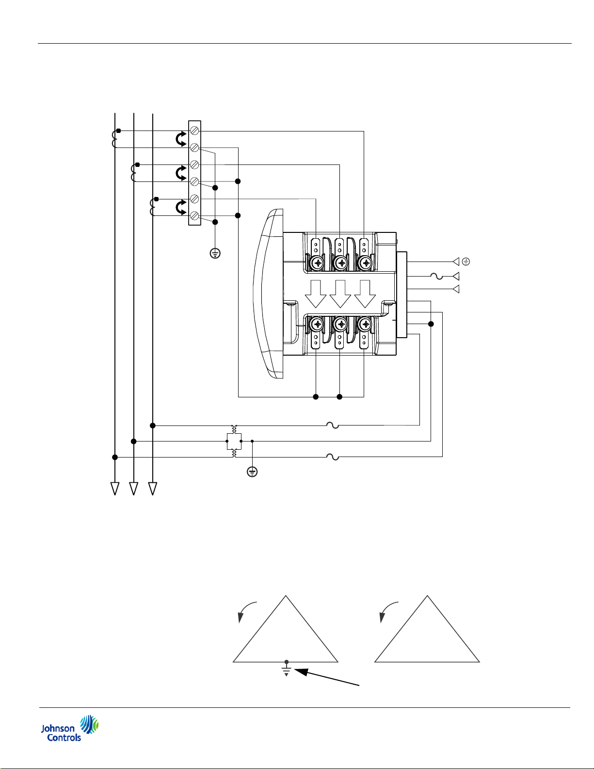
3. Three-Phase, Four-Wire Wye/Delta with PTs, 3 Element

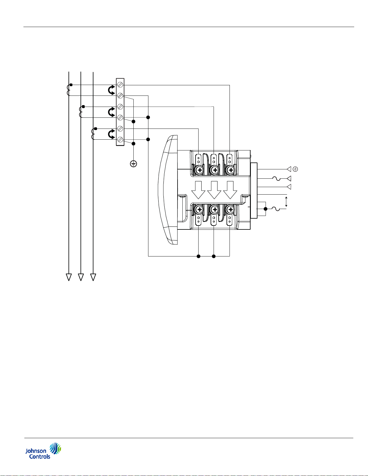
4. Three-Phase, Four-Wire Wye with PTs, 2.5 Element

5. Three-Phase, Three-Wire Delta with Direct Voltage

6. Three-Phase, Three-Wire Delta with 2 PTs, 2 CTs

7. Three-Phase, Three-Wire Delta with 2 PTs, 3 CTs

8. Current Only Measurement (Three Phase)

9. Current Only Measurement (Dual Phase)

10.Current Only Measurement (Single Phase)

WARNING: Risk of Electric Shock.
Disconnect the power supply before making electrical connections.
Contact with components carrying hazardous voltage can cause electric shock
and may result in severe personal injury or death.

AVERTISSEMENT: Risque de décharge électrique.

Débranchez l’alimentation électrique avant de faire un branchement électrique. Le contact
avec des composants ayant des tensons importantes peut provoquer une décharge
électrique, des blessures personnelles graves ou la mort.

EM-4000 Series Meters Installation and Operation Manual

4-10

4: Electrical Installation

C

B

A

C

BA

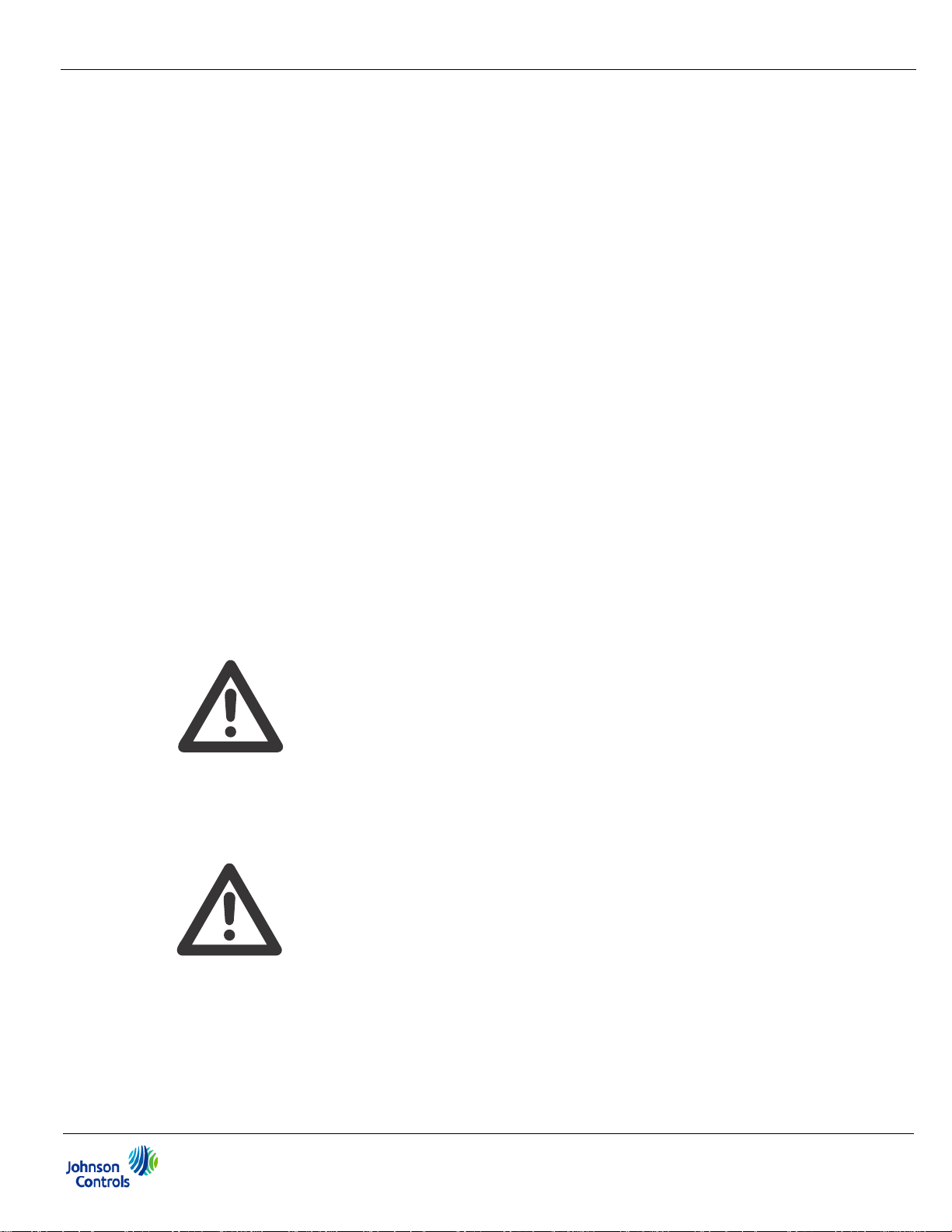
1. Service: WYE/Delta, 4-Wire with No PTs, 3 CTs

LINE

N

A

B

C

CT
Shorting
Block

Earth Ground

lc

LO

Power
Supply
Connection

GND

FUSE

HI

HI

HI

lb

la

LO

LO

L(+)

N(-)

Vref

Va

Vb

Vc

L(+)

3A

N(-)

FUSES
3 x 0.1A

N

A

LOAD

B

C

Select: “ 3 EL WYE ” (3 Element Wye) from the EM-4000 meter’s front panel display
(see Chapter 6).

EM-4000 Series Meters Installation and Operation Manual

4-11

1a. Example of Dual Phase Hookup

LINE

C

B

A

N

4: Electrical Installation

N

A

LOAD

CT
Shorting
Block

Earth Ground

HI

HI

HI

lb

lc

LO

FUSES
2 x 0.1A

C

B

la

LO

LO

GND

L(+)

N(-)

Vref

Va

Vb

Vc

x

Power
Supply
Connection

FUSE

3A

L(+)

N(-)

Select: “ 3 EL WYE ” (3 Element Wye) from the EM-4000 meter’s Front Panel Display.
(See Chapter 6.)

EM-4000 Series Meters Installation and Operation Manual

4-12

1b. Example of Single Phase Hookup

lc

HI

LO

lb

HI

LO

la

HI

LO

Earth Ground

x

L(+)

Power
Supply
Connection

N(-)

L(+)

GND

N(-)

Vref

Va

Vb

Vc

LINE

LOAD

CT
Shorting
Block

x

FUSE

0.1A

FUSE

3A

C

C

B

B

A

A

N

N

4: Electrical Installation

Select: “ 3 EL WYE ” (3 Element Wye) from the EM-4000 meter’s Front Panel Display.
(See Chapter 6.)

EM-4000 Series Meters Installation and Operation Manual

4-13

4: Electrical Installation

C

B

A

2. Service: 2.5 Element WYE, 4-Wire with No PTs, 3 CTs

LINE

N

A

B

C

CT
Shorting
Block

Earth Ground

lc

LO

Power
Supply
Connection

GND

FUSE

HI

HI

HI

lb

la

LO

LO

L(+)

N(-)

Vref

Va

Vb

Vc

L(+)

3A

N(-)

FUSES
2 x 0.1A

N

A

LOAD

B

C

Select: “2.5 EL WYE” (2.5 Element Wye) from the EM-4000 meter’s front panel
display (see Chapter 6).

EM-4000 Series Meters Installation and Operation Manual

4-14

4: Electrical Installation

lc

HI

LO

lb

HI

LO

la

HI

LO

Earth Ground

Earth Ground

L(+)

Power
Supply
Connection

N(-)

L(+)

GND

N(-)

Vref

Va

Vb

Vc

LINE

LOAD

CT
Shorting
Block

FUSES
3 x 0.1A

FUSE

3A

C

C

B

B

A

A

N

N

C

BA

C

B

A

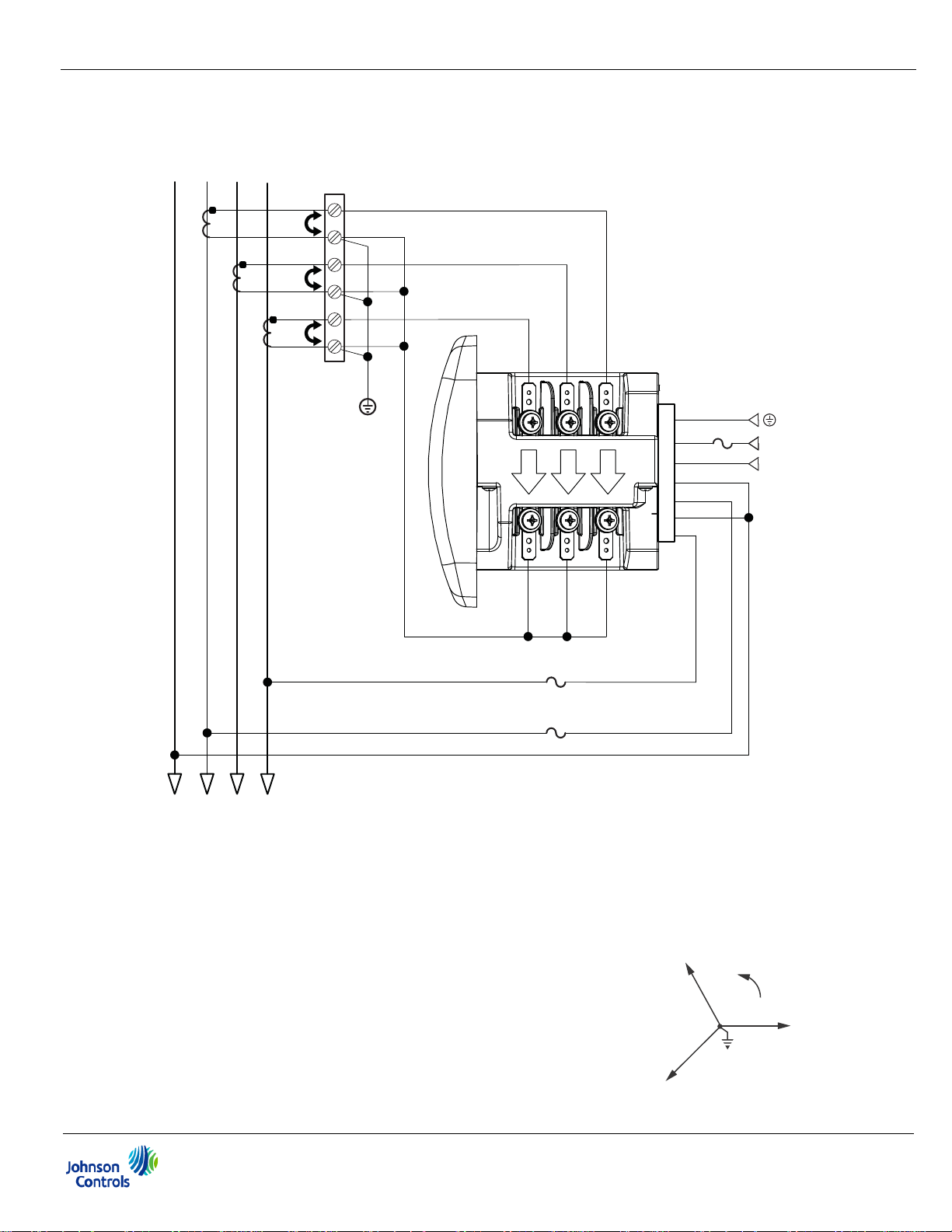
3. Service: WYE/Delta, 4-Wire with 3 PTs, 3 CTs

Select: “3 EL WYE” (3 Element Wye) from the EM-4000 meter’s front panel display
(see Chapter 6).

EM-4000 Series Meters Installation and Operation Manual

4-15

4: Electrical Installation

lc

HI

LO

lb

HI

LO

la

HI

LO

Earth Ground

Earth Ground

L(+)

Power
Supply
Connection

N(-)

L(+)

GND

N(-)

Vref

Va

Vb

Vc

LINE

LOAD

CT
Shorting
Block

FUSES
2 x 0.1A

FUSE

3A

C

C

B

B

A

A

N

N

C

B

A

4. Service: 2.5 Element WYE, 4-Wire with 2 PTs, 3 CTs

Select: “2.5 EL WYE” (2.5 Element Wye) from the EM-4000 meter’s front panel
display (see Chapter 6).

EM-4000 Series Meters Installation and Operation Manual

4-16

5. Service: Delta, 3-Wire with No PTs, 2 CTs

lc

HI

LO

lb

HI

LO

la

HI

LO

Earth Ground

L(+)

Power
Supply
Connection

N(-)

L(+)

GND

N(-)

Vref

Va

Vb

Vc

LINE

LOAD

CT
Shorting
Block

FUSES
3 x 0.1A

FUSE

3A

C

C

B

B

A

A

C

BA

C

BA

Not connected to meter

4: Electrical Installation

Select: “2 CT DEL” (2 CT Delta) from the EM-4000 meter’s front panel display (see
Chapter 6).

EM-4000 Series Meters Installation and Operation Manual

4-17

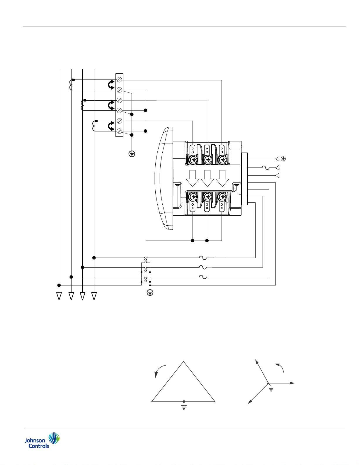
6. Service: Delta, 3-Wire with 2 PTs, 2 CTs

C

BA

C

BA

Not connected to meter

LINE

B

A

C

CT
Shorting
Block

4: Electrical Installation

A

LOAD

B

C

Earth Ground

Earth Ground

lc

HI

LO

FUSES
2 x 0.1A

lb

Power
Supply
Connection

GND

FUSE

HI

HI

la

LO

LO

L(+)

N(-)

Vref

Va

Vb

Vc

L(+)

3A

N(-)

Select: “2 CT DEL” (2 CT Delta) from the EM-4000 meter’s front panel display (see
Chapter 6).

EM-4000 Series Meters Installation and Operation Manual

4-18

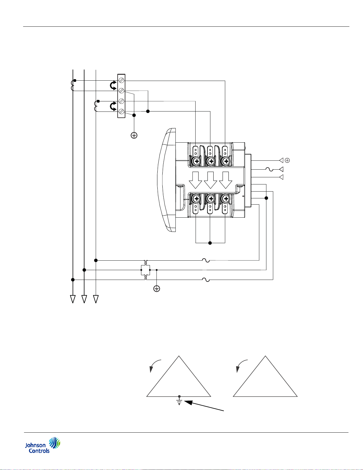
7. Service: Delta, 3-Wire with 2 PTs, 3 CTs

lc

HI

LO

lb

HI

LO

la

HI

LO

Earth Ground

Earth Ground

L(+)

Power
Supply
Connection

N(-)

L(+)

GND

N(-)

Vref

Va

Vb

Vc

LINE

LOAD

CT
Shorting
Block

FUSES
2 x 0.1A

FUSE

3A

C

C

B

B

A

A

C

BA

C

BA

Not connected to meter

4: Electrical Installation

Select: “2 CT DEL” (2 CT Delta) from the EM-4000 meter’s front panel display (see
Chapter 6).
NOTE: The third CT for hookup is optional, and is used only for Current
measurement.

EM-4000 Series Meters Installation and Operation Manual

4-19

4: Electrical Installation

lc

HI

LO

lb

HI

LO

la

HI

LO

Earth Ground

L(+)

Power
Supply
Connection

N(-)

L(+)

GND

N(-)

Vref

Va

Vb

Vc

LINE

LOAD

CT
Shorting
Block

FUSE

3A

FUSE

0.1A

20VAC
Minimum

C

C

B

B

A

A

8. Service: Current Only Measurement (Three Phase)

Select: “3 EL WYE” (3 Element Wye) from the EM-4000 meter’s front panel display
(see Chapter 6.)

* This connection is not required, but is recommended for improved accuracy.

EM-4000 Series Meters Installation and Operation Manual

4-20

4: Electrical Installation

lc

HI

LO

lb

HI

LO

la

HI

LO

Earth Ground

L(+)

Power
Supply
Connection

N(-)

L(+)

GND

N(-)

Vref

Va

Vb

Vc

LINE

LOAD

CT
Shorting
Block

FUSE

3A

FUSE

0.1A

20VAC
Minimum

B

B

A

A

9. Service: Current Only Measurement (Dual Phase)

Select: “3 EL WYE” (3 Element Wye) from the EM-4000 meter’s front panel display
(see Chapter 6).

* This connection is not required, but is recommended for improved accuracy.

EM-4000 Series Meters Installation and Operation Manual

4-21

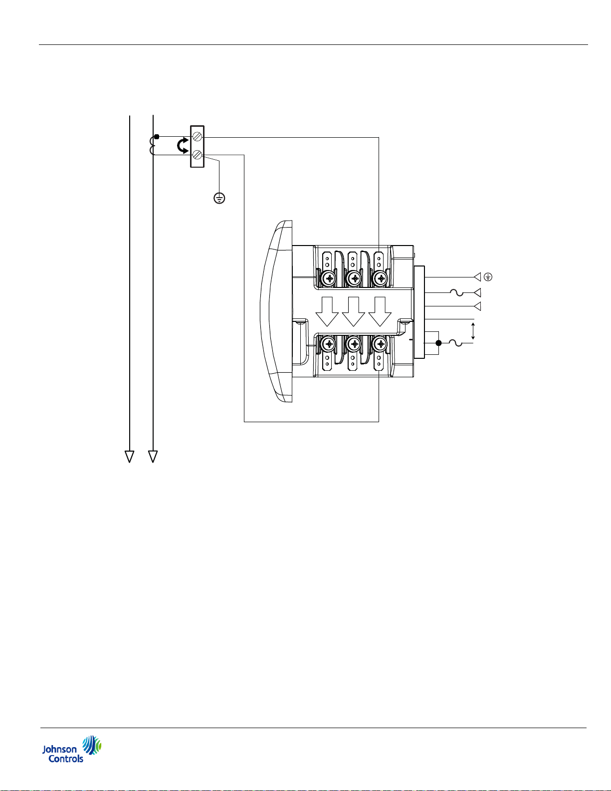
4: Electrical Installation

lc

HI

LO

lb

HI

LO

la

HI

LO

Earth Ground

L(+)

Power
Supply
Connection

N(-)

L(+)

GND

N(-)

Vref

Va

Vb

Vc

LINE

LOAD

CT
Shorting
Block

FUSE

3A

FUSE

0.1A

20VAC
Minimum

N

N

A

A

10. Service: Current Only Measurement (Single Phase)

Select: “3 EL WYE” (3 Element Wye) from the EM-4000 meter’s front panel display
(see Chapter 6).

* This connection is not required, but is recommended for improved accuracy.

NOTE: The diagram shows a connection to Phase A, but you can also connect to

Phase B or Phase C.

EM-4000 Series Meters Installation and Operation Manual

4-22

5: Communication Installation

5: Communication Installation

5.1: EM-4000 Series Meter Communication

The EM-4000 meter provides two independent Communication ports. The first port,
Com 1, is an optical IrDA port. The second port, Com 2, provides RS485
communication speaking Modbus® ASCII and Modbus® RTU protocols.

5.1.1: IrDA Port (Com 1)

The EM-4000 meter’s Com 1 IrDA port is on the face of the meter. The IrDA port
allows the unit to be read and programmed without the need of a communication
cable. Just point at the meter with an IrDA-equipped laptop PC to configure it.

NOTES:

• Settings for Com 1 (IrDA Port) are configured using the EM Series Communicator

Software.

• This port only communicates via Modbus® ASCII Protocol.

• Refer to Appendix D for instructions on using EIG’s USB to IrDA Adapter.

5.1.2: RS485 / KYZ Output (Com 2)

Com 2 provides a combination RS485 and an Energy Pulse Output (KYZ pulse).

See Chapter 2, Section 2.2 for the KYZ Output specifications; see Chapter 6, Section

6.4 for pulse constants.

EM-4000 Series Meters Installation and Operation Manual

5-1

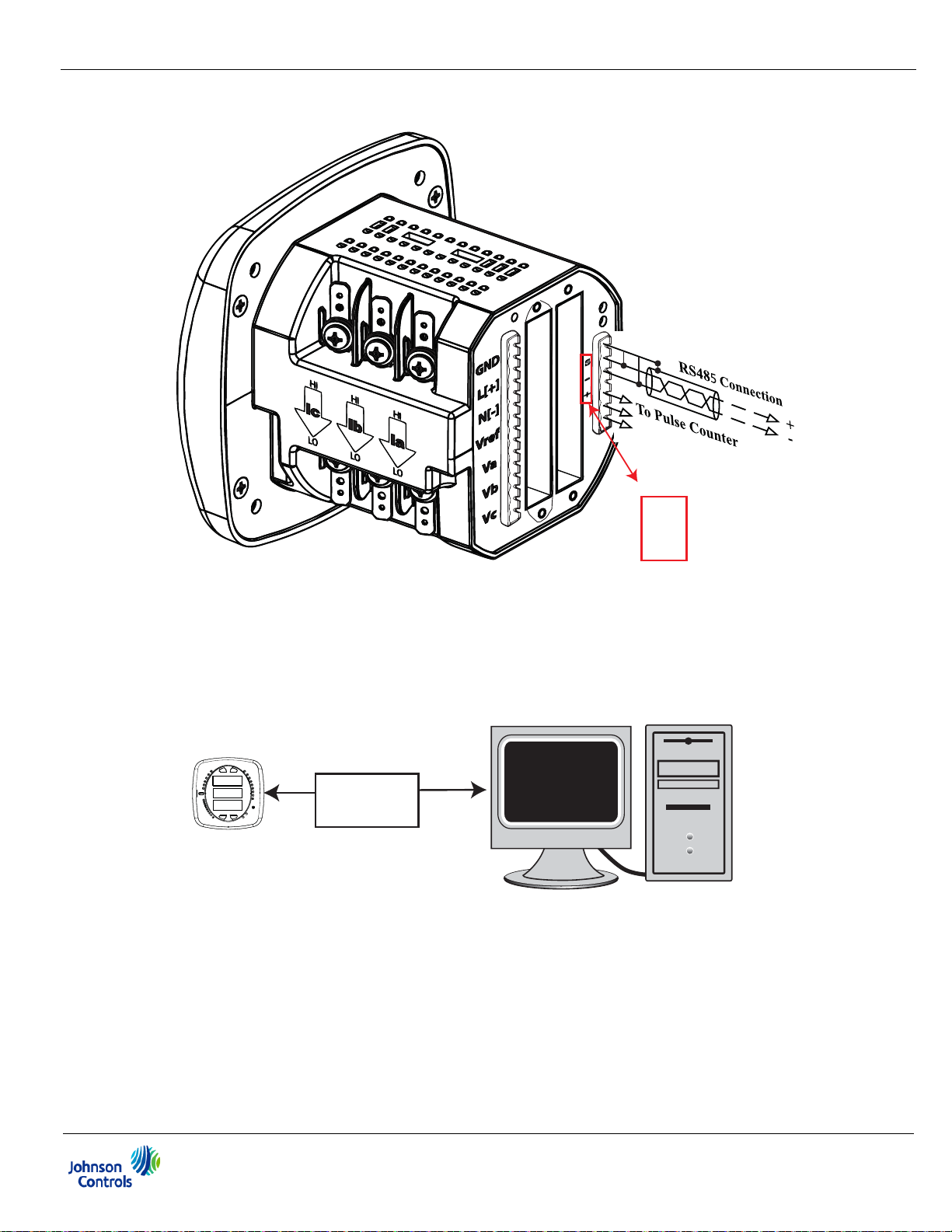
5: Communication Installation

Shield

-

+

Meter’s RS485 ConnectionsMeter’s RS485 Connections

Figure 5.1: EM-4000 Meter Back with RS485 Communication Installation

RS485 allows you to connect one or multiple EM-4000 meters to a PC or other device,
at either a local or remote site. All RS485 connections are viable for up to 4000 feet
(1219.20 meters).

120.00

120.00

120.00

EM-4000 meter

Figure 5.2: EM-4000 Meter Connected to a PC via RS485 bus

RS485

RS485/RS232
or RS485/USB
Converter

RS232
or USB

As shown in Figure 5.2, to connect an EM-4000 meter to a PC, you need to use either
an RS485 to RS232 or an RS485 to USB converter.

EM-4000 Series Meters Installation and Operation Manual

5-2

5: Communication Installation

MAX

MIN

VOLTS L-N

AMPS

%LOAD

120%-

PRG

%THD

LM2

LM1

90%-

60%-

30%-

VOLTS L-N

W/VAR/PF

VA/Hz

Wh

KILO

VARh

VAh

Wh Pulse

MEGA

A

B

C

MENU

ENTER

From other RS485 device

Connect :

•

(−) to (

−

)

•

(+) to (+)

•

Shield(SH) to Shield(SH)

EM-4000 meter RS485 connections

120

. 0

120 . 0

120 . 0

+

-

SH

+

-

SH

Figure 5.3 shows the detail of a 2-wire RS485 connection

Figure 5.3: 2-wire RS485 Connections to EM-4000 Meter

NOTES:

For All RS485 Connections:

• Use a shielded twisted pair cable and ground the shield, preferably at one location

only.

• Establish point-to-point configurations for each device on a RS485 bus: connect (+)

terminals to (+) terminals; connect (-) terminals to (-) terminals.

• You may connect up to 31 meters on a single bus using RS485. Before assembling

the bus, each meter must have a unique address: refer to the EM Series Communi-
cator Software User Manual for instructions.

• Protect cables from sources of electrical noise.

• Avoid both “Star” and “Tee” connections (see Figure 5.5).

• No more than two cables should be connected at any one point on an RS485 net-

work, whether the connections are for devices, converters, or terminal strips.

• Include all segments when calculating the total cable length of a network. If you are

not using an RS485 repeater, the maximum length for cable connecting all devices
is 4000 feet (1219.20 meters).

• Connect shield to RS485 Master and individual devices as shown in Figure 5.4. You

may also connect the shield to earth-ground at one point.

• Termination Resistors (RT) may be needed on both ends for longer length transmis-

sion lines. However, since the meter has some level of termination internally,

EM-4000 Series Meters Installation and Operation Manual

5-3

5: Communication Installation

Twisted pair, shielded (SH) cable

R

T

+ - SH

R

T

+ - SH

+ - SH

+ - SH

Slave device 1

Slave device 2

Last Slave device N Master device

Earth Connection, preferably at
single location

Twisted pair, shielded (SH) cable Twisted pair, shielded (SH) cable

g

p

p

Termination Resistors may not be needed. When they are used, the value of the
Termination Resistors is determined by the electrical parameters of the cable.

Figure 5.4 shows a representation of an RS485 Daisy Chain connection.

Figure 5.4: RS485 Daisy Chain Connection

R

+ - SH

Earth Connection, preferably at
sin

le location

Slave device 1

+ - SH

Long stub results “T” connection that can cause
interference

Twisted pair, shielded (SH) cable

Twisted pair, shielded (SH) cable Twisted pair, shielded (SH) cable

Slave device 1 Slave device 2

+ - SH

+ - SH + -SH

Slave device 3 Slave device 4

Twisted pair, shielded (SH) cable Twisted pair, shielded (SH) cable

Master device

roblem!

+ -SH

Slave device 2

+ - SH

+- SH

“STAR” connection can cause interference

roblem!

Last Slave device N Master device

R

+ - SH

Twisted pair, shielded (SH) cable

Twisted pair, shielded (SH) cable

Figure 5.5: Incorrect “T” and “Star” Topologies

EM-4000 Series Meters Installation and Operation Manual

5-4

6: Using the EM-4000 Meter

MAX

MIN

VOLTS L-N

AMPS

%LOAD

120%-

PRG

%THD

LM2

LM1

90%-

60%-

30%-

VOLTS L-N

W/VAR/PF

VA/Hz

Wh

KILO

VARh

VAh

Wh Pulse

MEGA

A

B

C

MENU

ENTER

IrDA

0000

0.659

IrDA Com

Port

Reading

Type

Indicator

Parameter

Designator

Watt-hour

Test P ul se

Scaling

Factor

% of Load

Bar

6.1: Introduction

You can use the Elements and Buttons on the EM-4000 meter’s face to view meter
readings, reset and/or configure the meter, and perform related functions. The follow­ing sections explain the Elements and Buttons and detail their use.

6.1.1: Understanding Meter Face Elements

6: Using the EM-4000 Meter

The meter face features the following elements:

• Reading type indicator: e.g., Max

• Parameter designator: e.g., Volts L-N

• Watt-hour test pulse: Energy pulse output to test accuracy

• Scaling factor: Kilo or Mega multiplier of displayed readings

• % of Load bar: Graphic Display of Amps as % of the load (see Section 6.3 for

additional information)

• IrDA Communication port: Com 1 port for wireless communication

Figure 6.1: Face Plate with Elements

EM-4000 Series Meters Installation and Operation Manual

6-1

6.1.2: Understanding Meter Face Buttons

MAX

MIN

VOLTS L-N

AMPS

%LOAD

120%-

PRG

%THD

LM2

LM1

90%-

60%-

30%-

VOLTS L-N

W/VAR/PF

VA/Hz

Wh

KILO

VARh

VAh

Wh Pulse

MEGA

A

B

C

MENU

ENTER

IrDA

0000

0.659

Menu Enter

Down Right

6: Using the EM-4000 Meter

Figure 6.2: Faceplate with Buttons

The meter face has Menu, Enter, Down and Right buttons, which let you perform
the following functions:

• View meter information

• Enter display modes

• Configure parameters (may be Password protected)

• Perform resets (may be Password protected)

• Perform LED Checks

• Change settings

• View parameter values

• Scroll parameter values

• View Limit states

EM-4000 Series Meters Installation and Operation Manual

6-2

6.2: Using the Front Panel

You can access four modes using the EM-4000 meter’s front panel buttons:

• Operating mode (Default)

• Reset mode

• Configuration mode

• Information mode - Information mode displays a sequence of screens that show

model information, such as Frequency, Amps, V-Switch, etc.

Use the Menu, Enter, Down and Right buttons to navigate through each mode and
its related screens.

NOTES:

6: Using the EM-4000 Meter

• See Appendix A for the display’s Navigation maps.

• The meter can also be configured using software; see the EM Series Communicator

Software User Manual for instructions.

6.2.1: Understanding Startup and Default Displays

Upon powering up, the meter displays a sequence of screens:

• Lamp Test screen where all LEDs are lit

• Lamp Test screen where all digits are lit

• Firmware screen showing the build number

• Error screen (if an error exists)

After startup, if auto-scrolling is enabled, the EM-4000 meter scrolls the parameter
readings on the right side of the front panel. The Kilo or Mega LED lights, showing the
scale for the Wh, VARh and VAh readings. Figure 6.3 shows an example of a Wh
reading.

EM-4000 Series Meters Installation and Operation Manual

6-3

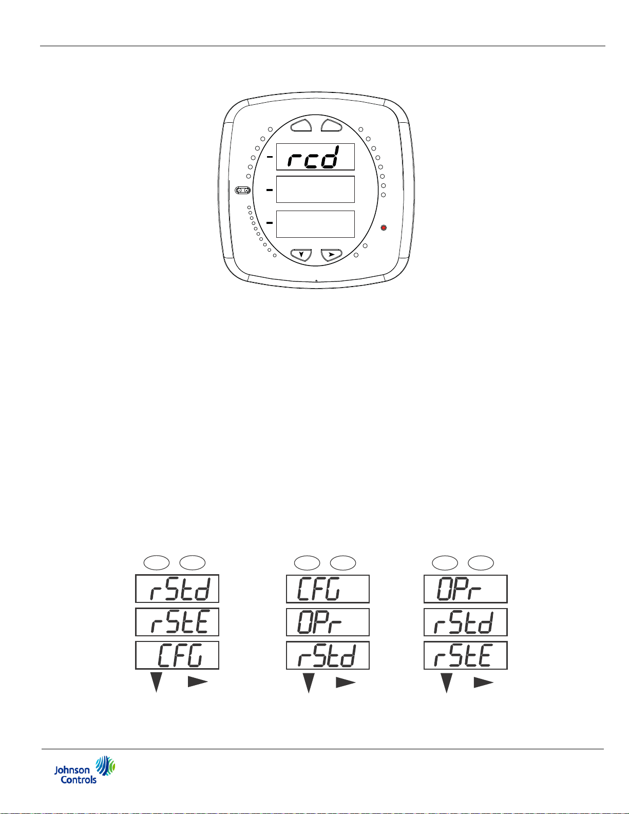
6: Using the EM-4000 Meter

MAX

MIN

VOLTS L-N

AMPS

%LOAD

120%-

PRG

%THD

LM2

LM1

90%-

60%-

30%-

VOLTS L-N

W/VAR/PF

VA/Hz

Wh

KILO

VARh

VAh

Wh Pulse

MEGA

A

B

C

MENU

ENTER

IrDA

0000

0.659

A

B

C

-

-

-

MENU ENTER

A

B

C

-

-

-

MENU ENTER

A

B

C

-

-

-

MENU ENTER

Figure 6.3: Display Showing Watt-hour Reading

The EM-4000 meter continues to provide scrolling readings until one of the buttons on
the front panel is pressed, causing the meter to enter one of the other Modes.

6.2.2: Using the Main Menu

1. Press the Menu button. The Main Menu screen appears.

• The Reset: Demand mode (rStd) appears in the A window. Use the Down button to

scroll, causing the Reset: Energy (rStE), Configuration (CFG), Operating (OPr), and
Information (InFo) modes to move to the A window.

• The mode that is currently flashing in the A window is the “Active” mode, which

means it is the mode that can be configured.

For example: Press Down Twice - CFG moves to A window. Press Down Twice - OPr moves to

A window.

EM-4000 Series Meters Installation and Operation Manual

6-4

2. Press the Enter button from the Main Menu to view the Parameters screen for the

A

B

C

-

-

-

MENU ENTER

A

B

C

-

MENU ENTER

A

B

C

-

-

-

MENU ENTER

A

B

C

-

-

-

MENU ENTER

mode that is currently active.

6.2.3: Using Reset Mode

Reset Mode has two options:

• Reset: Demand (rStd): resets the Max and Min values

• Reset: Energy (rStE): resets the energy accumulator fields

1. Press the Enter button while

either rStd or rStE is in the A win­dow. The Reset Demand No or
Reset Energy No screen appears.

• If you press the Enter button

6: Using the EM-4000 Meter

-

-

again, the Main Menu appears,
with the next mode in the A
window. (The Down button
does not affect this screen.)

• If you press the Right button,

the Reset Demand YES or
Reset Energy YES screen
appears. Press Enter to per­form a reset.

NOTE: If Password protection is enabled for reset, you must enter the four digit
password before you can reset the meter. (See the EM Series Communicator Software
User Manual for information on Password protection.) To enter a password, follow the
instructions in Section 6.2.4.

CAUTION! Reset Demand YES resets all Max and Min values.

2. Once you have performed a reset, the screen displays either “rSt dMd donE” or

“rSt EnEr donE”and then resumes auto-scrolling parameters.

EM-4000 Series Meters Installation and Operation Manual

6-5

6.2.4: Entering a Password

A

B

C

-

MENU ENTER

A

B

C

-

MENU ENTER

PASS
12__

A

B

C

-

MENU ENTER

If Password Protection has been enabled in the software for reset and/or configuration
(see the EM Series Communicator Software User Manual for more information), a
screen appears requesting a password when you try to reset the meter and/or config­ure settings through the front panel.

• PASS appears in the A window and 4 dashes appear in the B window; the left-most

dash is flashing.

1. Press the Down button to scroll numbers from 0 to 9 for the flashing dash. When

the correct number appears for that dash, use the Right button to move to the
next dash.

Example: The left screen, below, shows four dashes. The right screen shows the
display after the first two digits of the password have been entered.

6: Using the EM-4000 Meter

-

-

2. When all 4 digits of the password have been selected, press the Enter button.

• If you are in Reset mode and you enter the correct password, “rSt dMd donE” or
“rSt EnEr donE”appears and the screen resumes auto-scrolling parameters.

• If you are in Configuration mode and you enter the correct password, the display

returns to the screen that required a password.

• If you enter an incorrect Password, “PASS ----

FAIL” appears and:

• The previous screen is redisplayed, if you
are in Reset mode.

• The previous Operating mode screen is

-

-

-

-

redisplayed, if you are in Configuration
mode.

EM-4000 Series Meters Installation and Operation Manual

6-6

6.2.5: Using Configuration Mode

A

B

C

-

MENU ENTER

A

B

C

-

MENU ENTER

Configuration mode follows Reset: Energy on the Main Menu.

To access Configuration mode:

1. Press the Menu button while the meter is auto-scrolling parameters.

2. Press the Down button until the Configuration mode option (CFG) is in the A

window.

3. Press the Enter button. The configuration Parameters screen appears.

4. Press the Down button to scroll through the configuration parameters: Scroll

(SCrL), CT, PT, Connection (Cnct) and Port. The parameter currently ‘Active,” i.e.,
configurable, flashes in the A window.

6: Using the EM-4000 Meter

5. Press the Enter button to access the Setting screen for the currently active param-

eter.

NOTE: You can use the Enter button to scroll through all of the configuration
parameters and their Setting screens, in order.

-

-

Press Enter when CFG is in A window - Parameter screen appears ­ Press Down- Press Enter when

Parameter you want is in A window

-

-

6. The parameter screen appears, showing the current settings. To change the
settings:

• Use either the Down button or the Right button to select an option.

EM-4000 Series Meters Installation and Operation Manual

6-7

6: Using the EM-4000 Meter

A

B

C

-

MENU ENTER

A

B

C

-

MENU ENTER

A

B

C

-

MENU ENTER

• To enter a number value, use the Down button to select the number value for a

digit and the Right button to move to the next digit.

NOTE: When you try to change the current setting and Password protection is
enabled for the meter, the Password screen appears. See Section 6.2.4 for instruc­tions on entering a password.

7. Once you have entered the new setting, press the Menu button twice.

8. The Store ALL YES screen appears. You can either:

• Press the Enter button to save the new setting.

• Press the Right button to access the Store ALL no screen; then press the Enter

button to cancel the Save.

9. If you have saved the settings, the Store ALL done screen appears and the meter
resets.

-

-

Press the Enter button to save Press the Enter button to The settings have been
the settings. Press the Right Cancel the Save. saved.

button for Stor All no screen.

-

-

-

-

EM-4000 Series Meters Installation and Operation Manual

6-8

6.2.5.1: Configuring the Scroll Feature

A

B

C

-

MENU ENTER

A

B

C

-

-

-

MENU ENTER

When in auto-scrolling mode, the meter performs a scrolling display, showing each
parameter for 7 seconds, with a 1 second pause between parameters. The parameters
that the meter displays are determined by the following conditions:

• They have been selected through software (see the EM Series Communicator Soft-
ware User Manual for instructions).

6: Using the EM-4000 Meter

• They are enabled by the installed V-Switch

TM

on V-Switch

keys).

TM

key (see Section 2.1.3 for information

To enable or disable auto-scrolling:

1. Press the Enter button when SCrl is in the A window.
The Scroll YES screen appears.

2. Press either the Right or Down button if you want to
access the Scroll no screen. To return to the Scroll
YES screen, press either button.

3. Press the Enter button on either the Scroll YES
screen (to enable auto-scrolling) or the Scroll no
screen (to disable auto-scrolling).

4. The CT- n screen appears (this is the next Configura­tion mode parameter).

-

-

NOTES:

• To exit the screen without changing scrolling options, press the Menu button.

• To return to the Main Menu screen, press the Menu button twice.

• To return to the scrolling (or non-scrolling) parameters display, press the Menu
button three times.

EM-4000 Series Meters Installation and Operation Manual

6-9

6.2.5.2: Configuring CT Setting

The CT Setting has three parts: Ct-n (numerator), Ct-d (denominator), and Ct-S
(scaling).

1. Press the Enter button when Ct is in the A window. The Ct-n screen appears. You
can either:

• Change the value for the CT numerator.

• Access one of the other CT screens by pressing the Enter button: press Enter

once to access the Ct-d screen, twice to access the Ct-S screen.

NOTE: The Ct-d screen is preset to a 5 Amp value at the factory and cannot be

changed.

a. To change the value for the CT numerator:

6: Using the EM-4000 Meter

From the Ct-n screen:

• Use the Down button to select the number value for a digit.

• Use the Right button to move to the next digit.

b. To change the value for CT scaling:

From the Ct-S screen, use the Right button or the Down button to choose the
scaling you want. The Ct-S setting can be 1, 10, or 100.

NOTE: If you are prompted to enter a password, refer to Section 6.2.4 for instruc­tions on doing so.

2. When the new setting is entered, press the Menu button twice.

3. The Store ALL YES screen appears. Press Enter to save the new CT setting.

Example CT Settings:

200/5 Amps: Set the Ct-n value for 200 and the Ct-S value for 1.

800/5 Amps: Set the Ct-n value for 800 and the Ct-S value for 1.

2,000/5 Amps: Set the Ct-n value for 2000 and the Ct-S value for 1.

10,000/5 Amps: Set the Ct-n value for 1000 and the Ct-S value for 10.

EM-4000 Series Meters Installation and Operation Manual

6-10

6: Using the EM-4000 Meter

A

B

C

-

-

-

MENU ENTER

A

B

C

-

MENU ENTER

A

B

C

-

-

-

MENU ENTER

A

B

C

-

-

-

MENU ENTER

NOTES:

• The value for Amps is a product of the Ct-n value and the Ct-S value.

• Ct-n and Ct-S are dictated by primary current; Ct-d is secondary current.

-

-

Press Enter Use buttons to set Ct-n Ct-d cannot be changed Use buttons to select
scaling

6.2.5.3: Configuring PT Setting

The PT Setting has three parts: Pt-n (numerator), Pt-d (denominator), and Pt-S (scal­ing).

1. Press the Enter button when Pt is in the A window. The PT-n screen appears. You
can either:

• Change the value for the PT numerator.

• Access one of the other PT screens by pressing the Enter button: press Enter

once to access the Pt-d screen, twice to access the Pt-S screen.

a. To change the value for the PT numerator or denominator:

From the Pt-n or Pt-d screen:

• Use the Down button to select the number value for a digit.

• Use the Right button to move to the next digit.

b. To change the value for the PT scaling:

From the Pt-S screen, use the Right button or the Down button to choose the
scaling you want. The Pt-S setting can be 1, 10, 100, or 1000.

NOTE: If you are prompted to enter a password, refer to Section 6.2.4 for instruc­tions on doing so.

EM-4000 Series Meters Installation and Operation Manual

6-11

6: Using the EM-4000 Meter

A

B

C

-

MENU ENTER

A

B

C

-

-

-

MENU ENTER

A

B

C

-

MENU ENTER

2. When the new setting is entered, press the Menu button twice.

3. The STOR ALL YES screen appears. Press Enter to save the new PT setting.

Example PT Settings:

277/277 Volts: Pt-n value is 277, Pt-d value is 277, Pt-S value is 1.

14,400/120 Volts: Pt-n value is 1440, Pt-d value is 120, Pt-S value is 10.

138,000/69 Volts: Pt-n value is 1380, Pt-d value is 69, Pt-S value is 100.

345,000/115 Volts: Pt-n value is 3450, Pt-d value is 115, Pt-S value is 100.

345,000/69 Volts: Pt-n value is 345, Pt-d value is 69, Pt-S value is 1000.

NOTE: Pt-n and Pt-S are dictated by primary voltage; Pt-d is secondary voltage.

-

-

Use buttons to set Pt-n Use buttons to set Pt-d Use buttons to select scaling

-

-

EM-4000 Series Meters Installation and Operation Manual

6-12

6.2.5.4: Configuring Connection Setting

A

B

C

-

MENU ENTER

1. Press the Enter button when Cnct is in the A window. The Cnct screen appears.

2. Press the Right button or Down button to select a configuration. The choices are:

• 3 Element Wye (3 EL WYE)

• 2.5 Element Wye (2.5EL WYE)

• 2 CT Delta (2 Ct dEL)

NOTE: If you are prompted to enter a password, refer to Section 6.2.4 for instruc­tions on doing so.

3. When you have made your selection, press the Menu button twice.

6: Using the EM-4000 Meter

4. The STOR ALL YES screen appears. Press Enter to save the setting.

-

-

Use buttons to select configuration

6.2.5.5: Configuring Communication Port Setting

Port configuration consists of: Address (a three digit number), Baud Rate (9600;
19200; 38400; or 57600), and Protocol (Modbus® RTU or Modbus® ASCII).

1. Press the Enter button when POrt is in the A window. The Adr (address) screen
appears. You can either:

• Enter the address.

• Access one of the other Port screens by pressing the Enter button: press Enter

once to access the bAUd screen (Baud Rate), twice to access the Prot screen
(Protocol).

EM-4000 Series Meters Installation and Operation Manual

6-13

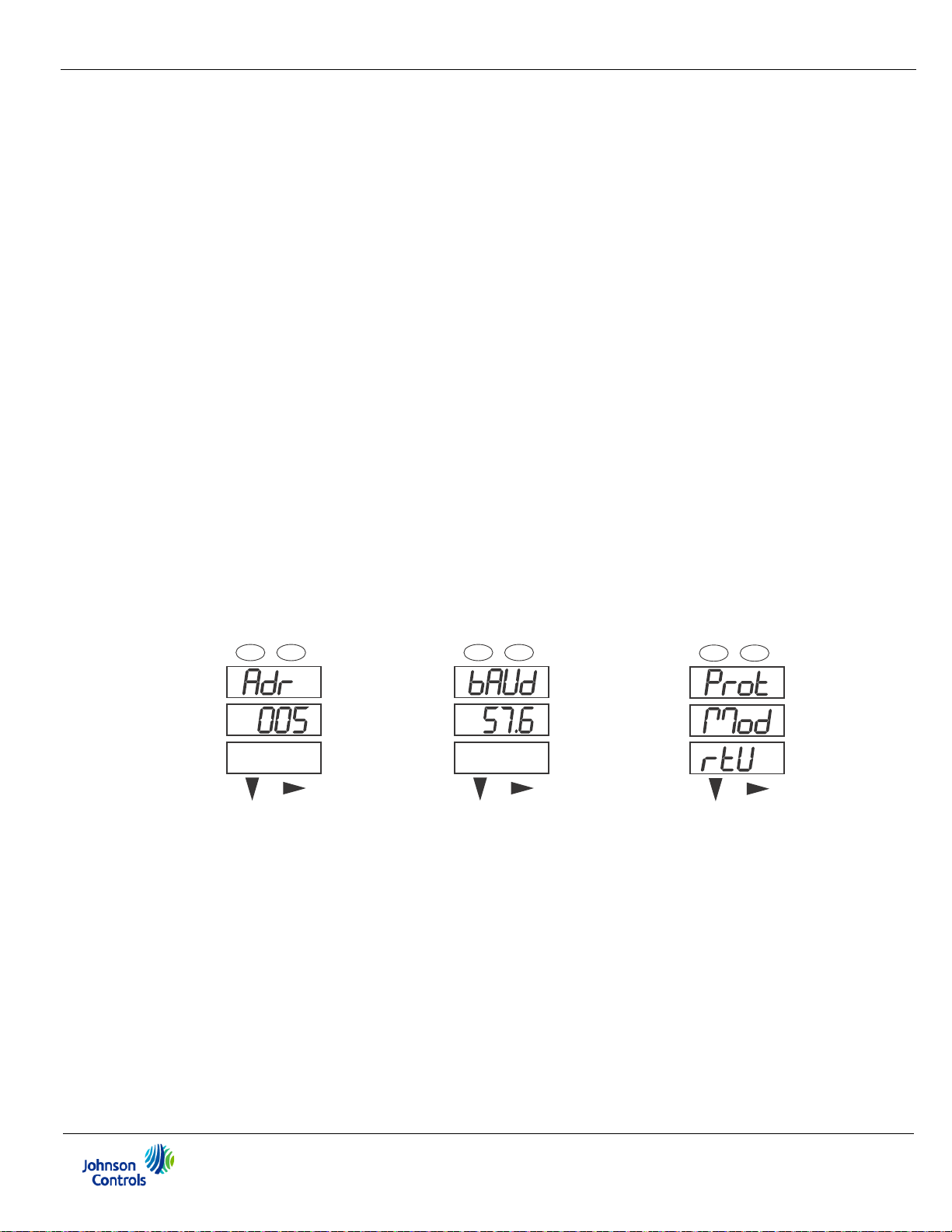
6: Using the EM-4000 Meter

A

B

C

-

-

-

MENU ENTER

A

B

C

-

MENU ENTER

A

B

C

-

-

-

MENU ENTER

a. To enter the Address:

From the Adr screen:

• Use the Down button to select the number value for a digit.

• Use the Right button to move to the next digit.

b. To select the Baud Rate:

From the bAUd screen, use the Right button or the Down button to select the
setting you want.

c. To select the Protocol:

From the Prot screen, press the Right button or the Down button to select the
setting you want.

NOTE: If you are prompted to enter a password, refer to Section 6.2.4 for instruc­tions on doing so.

2. When you have finished making your selections, press the Menu button twice.

3. The STOR ALL YES screen appears. Press Enter to save the settings.

-

-

Use buttons to enter Address Use buttons to select Baud Rate Use buttons to select Protocol

EM-4000 Series Meters Installation and Operation Manual

6-14

6.2.6: Using Operating Mode

Operating mode is the EM-4000 meter’s default mode, that is, the standard front
panel display. After starting up, the meter automatically scrolls through the parameter
screens, if scrolling is enabled. Each parameter is shown for 7 seconds, with a 1 sec­ond pause between parameters. Scrolling is suspended for 3 minutes after any button
is pressed.

1. Press the Down button to scroll all the parameters in Operating mode. The
currently “Active,” i.e., displayed, parameter has the Indicator light next to it, on
the right face of the meter.

2. Press the Right button to view additional readings for that parameter. The table
below shows possible readings for Operating Mode. Sheet 2 in Appendix A shows
the Operating mode Navigation map.

6: Using the EM-4000 Meter

NOTE: Readings or groups of readings are skipped if not applicable to the meter type
or hookup, or if they are disabled in the programmable settings.

OPERATING MODE PARAMETER READINGS

POSSIBLE READINGS

VOLTS L-N VOLTS_LN VOLTS_LN_

MAX

VOLTS L-L VOLTS_LL VOLTS_LL_MAX VOLTS_LL_MIN

AMPS AMPS AMPS_NEUTRAL AMPS_MAX AMPS_MIN AMPS_THD

W/VAR/PF W_VAR_PF W_VAR_PF_MA

X_POS

VA/Hz VA_FREQ VA_FREQ_MAX VA_FREQ_MIN

Wh KWH_REC KWH_DEL KWH_NET KWH_TOT

VARh KVARH_POS KVARH_NEG KVARH_NET KVARH_TOT

VAh KVAH

VOLTS_LN_
MIN

W_VAR_PF_MIN
_POS

VOLTS_LN_
THD

W_VAR_PF_
MIN_NEG

EM-4000 Series Meters Installation and Operation Manual

6-15

6.3: Understanding the % of Load Bar

0000

-

-

-

A

B

C

MENU ENTER

MAX

MIN

LM1

LM2

%THD

PRG

VOLTS L-N

VOLTS L-L

AMPS

WNARP

VA/Hz

lrDA

Wh

VARh

VAh

120%-

90%-

60%-

30%-

%LOAD

MEGA

KILO

Wh Pulse

10

The 10-segment LED bar graph at the bottom left of the EM-4000 meter’s front panel
provides a graphic representation of Amps. The segments light according to the load,
as shown in the table below.
When the load is over 120% of Full Load, all segments flash “On” (1.5 secs) and “Off”
(0.5 secs).

Segments Load >= % Full Load

none no load

11%

1-2 15%

1-3 30%

1-4 45%

6: Using the EM-4000 Meter

1-5 60%

1-6 72%

1-7 84%

1-8 96%

1-9 108%

1-10 120%

All Blink >120%

The % of Load bar can be programmed through EM Series Communicator Software ­see the EM Series Communicator Software User Manual for instructions.

1

EM-4000 Series Meters Installation and Operation Manual

6-16

6: Using the EM-4000 Meter

MAX

MIN

VOLTS L-N

AMPS

%LOAD

120%-

PRG

%THD

LM2

LM1

90%-

60%-

30%-

VOLTS L-N

W/VAR/PF

VA/Hz

Wh

KILO

VARh

VAh

Wh Pulse

MEGA

A

B

C

MENU

ENTER

IrDA

0000

0.659

Watt-hour
test pulse

6.4: Performing Watt-Hour Accuracy Testing (Verification)

To be certified for revenue metering, power providers and utility companies must
verify that the billing energy meter performs to the stated accuracy. To confirm the
meter’s performance and calibration, power providers use field test standards to
ensure that the unit’s energy measurements are correct. Since the EM-4000 meter is
a traceable revenue meter, it contains a utility grade test pulse that can be used to
gate an accuracy standard. This is an essential feature required of all billing grade
meters.

• Refer to Figure 6.5 for an example of how this process works.

• Refer to Table 6.1 for the Wh/Pulse constants for accuracy testing.

Figure 6.4: Watt-hour Test Pulse

EM-4000 Series Meters Installation and Operation Manual

6-17

6: Using the EM-4000 Meter

-

-

-

A

B

C

MENU ENTER

MAX

MIN

LM1

LM2

%THD

PRG

VOLTS L-N

VOLTS L-L

AMPS

WNARP

VA/Hz

lrDA

Wh

VARh

VAh

120%-

90%-

60%-

30%-

%LOAD

MEGA

KILO

Wh Pulse

Comparator

Energy

Standard

Error

Results

Test Pulses Energy Pulses

Figure 6.5: Using the Watt-hour Test Pulse

Input Voltage Level EM-4000 Meter

Below 150V 0.500017776

Above 150V 2.000071103

Table 6.1: Infrared & KYZ Pulse Constants for Accuracy Testing - Kh Watt-hour per pulse

NOTES:

• Minimum pulse width is 90 milliseconds.

• Refer to Chapter 2, Section 2.2, for Wh Pulse specifications.

EM-4000 Series Meters Installation and Operation Manual

6-18

7: Data Logging

7.1: Overview

The EM-4000 meter has 2 MB of flash memory for data logging. The meter can log
historical trends, and sequence of events. In addition, the meter has a real-time clock
that allows all events to be time-stamped when they occur.

7.2: Available Logs

The following logs are available for the EM-4000 meter.

• Historical logs: The EM-4000 meter has three Historical logs. Each log can be inde­pendently programmed with individual trending profiles, that is, each can be used
to measure different values. You can program up to 64 parameters per log. You
also have the ability to allocate available system resources between the three logs,

7: Data Logging

to increase or decrease the size of the individual historical logs. See the EM Series
Communicator Software User Manual for additional information and instructions.

• System Events log: In order to protect critical billing information, the EM-4000
meter records and logs the following information with a timestamp:

• Demand resets

• Password requests

• System startup

• Energy resets

• Log resets

• Log reads

• Programmable settings changes

All of the EM-4000 meter logs can be viewed through the Log Viewer. Refer to the EM
Series Communicator Software User Manual for additional information and instruc­tions regarding logs and the Log Viewer.

EM-4000 Series Meters Installation and Operation Manual

7-1

7: Data Logging

This page intentionally left blank.

EM-4000 Series Meters Installation and Operation Manual

7-2

A: EM-4000 Meter Navigation Maps

A: EM-4000 Meter Navigation Maps

A.1: Introduction

You can configure the EM-4000 meter and perform related tasks using the buttons on
the meter face. Chapter 6 contains a description of the buttons on the meter face and
instructions for programming the meter using them. The meter can also be pro­grammed using software (see the EM Series Communicator Software User Manual).

A.2: Navigation Maps (Sheets 1 to 4)

The EM-4000 meter’s Navigation maps begin on the next page. The maps show in
detail how to move from one screen to another and from one Display mode to another
using the buttons on the face of the meter. All Display modes automatically return to
Operating mode after 10 minutes with no user activity.

EM-4000 Meter Navigation Map Titles:

• Main Menu screens (Sheet 1)

• Operating mode screens (Sheets 2)

• Reset mode screens (Sheet 3)

• Configuration mode screens (Sheet 4)

EM-4000 Series Meters Installation and Operation Manual

A-1

MAIN MENU Screen

MAIN MENU:

RSTD (blinking)
RSTE
CFG

DOWN

DOWN

MAIN MENU screen scrolls through 5 choices,

showing 3 at a time. The top choice is always the

"active" one, which is indicated by blinking the legend.

MAIN MENU:

CFG (blinking)
INFO
OPR

MAIN MENU:

OPR (blinking)
RSTD
RSTE

CONFIGURATION MODE

grid of meter settings screens with

password-protected edit capability.

See sheet 5

OPERATING MODE

grid of meter data screens.

See sheets 2 & 3

ENTER

STARTUP

sequence run once at meter startup:

2 lamp test screens, hardware information

screen, firmware version screen,

(conditional) error screens

sequence completed

RESET DEMAND MODE

sequence of screens to get password, if

required, and reset max/min data.

See sheet 4

single screen

all screens

for a display

mode

button

group of

screens

MENU

ENTER

DOWN, RIGHT

Navigation:

Editing:

Returns to previous menu from any screen in any mode

Indicates acceptance of the current screen and advances to the
next one

Navigation and edit buttons
No digits or legends are blinking. On a menu, down advances
to the next menu selection, right does nothing. In a grid of
screens, down advances to the next row, right advances to the
next column. Rows, columns, and menus all navigate circularly.
A digit or legend is blinking to indicate that it is eligible for
change. When a digit is blinking, down increases the digit
value, right moves to the next digit. When a legend is blinking,
either button advances to the next choice legend.

action taken

10 minutes

with no

user activity

Configuration Mode is not
available during a
Programmable Settings
update via a COM port.

MAIN MENU:

RSTE (blinking)
CFG
INFO

DOWN

ENTER

ENTER

ENTER

DOWN

RESET ENERGY MODE

sequence of screens to get password, if

required, and reset energy accumulators.

See sheet 4

MENU

MENU

MENU

MENU

10 minutes with no user activity

SYMBOLS BUTTONS

MAIN MENU:

INFO (blinking)
OPR
RSTD

DOWN

INFORMATION

sequence of screens to show model

information, same as STARTUP except

lamp tests omitted.

MENU

ENTER

sequence

completed

Reset Energy Mode is not
available for SHVA120,
SHAA5, or SHWA300.

Main Menu Screens (Sheet 1)

A: EM-4000 Meter Navigation Maps

EM-4000 Series Meters Installation and Operation Manual

A-2

A: EM-4000 Meter Navigation Maps

EM-4000 Series Meters Installation and Operation Manual

A-3

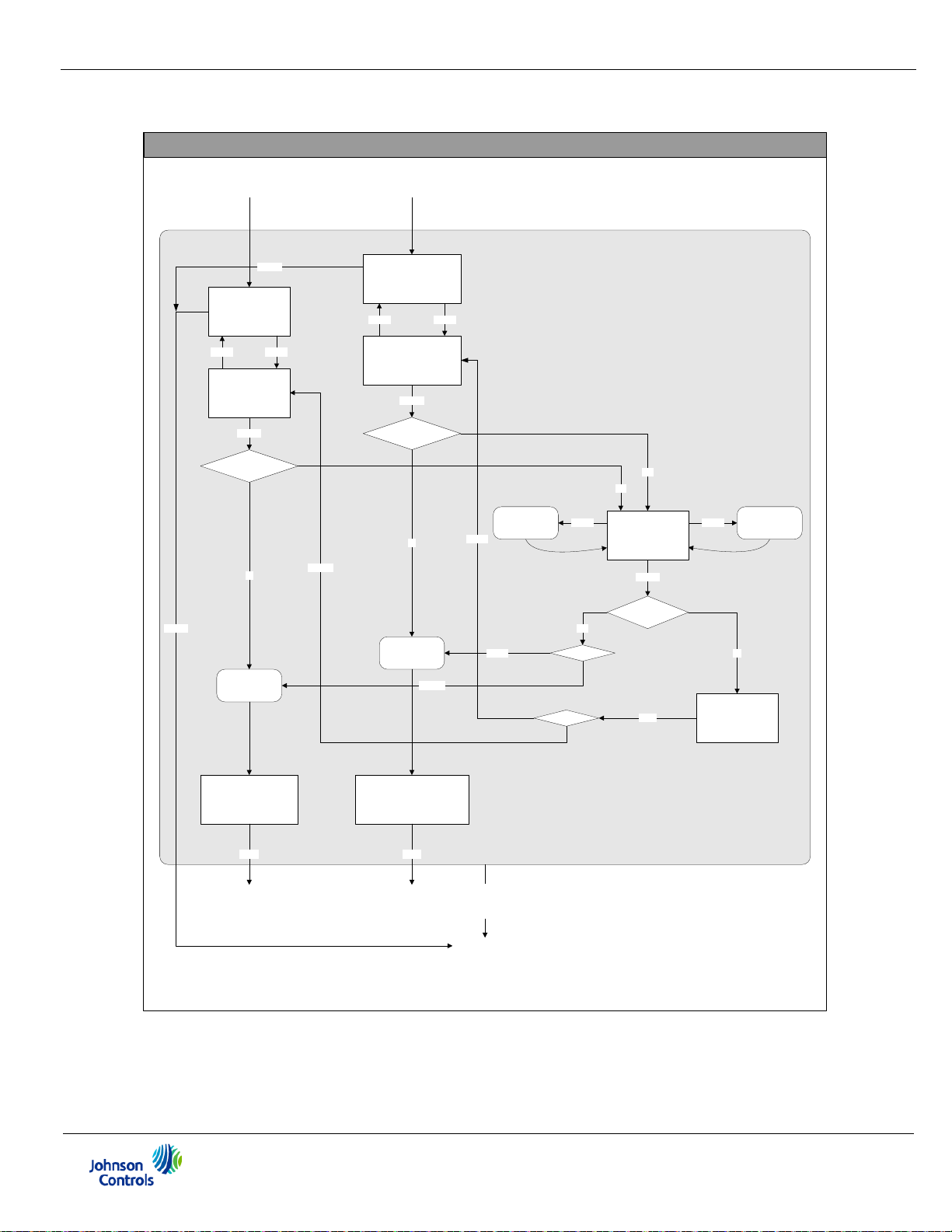
RESET_MM_NO:

RST
DMD
no (blinking)

is password required?

RIGHTRIGHT

ENTER

is password

correct?

ENTER

2 sec

RIGHTDOWN

RESET_MM_YES:

RST
DMD
yes (blinking)

reset all max &

min values

RESET_MM_CONFIRM:

RST
DMD
DONE

RESET_ENTER_PW:

PASS
#### (one # blinking)

make next digit

blink

increment

blinking digit

from MAIN MENU

(RSTD selected)

MENU

(from any

reset mode

screen)

RESET_PW_FAIL:

PASS
####
FAIL

no

ENTER

2 sec.

to previous operating

mode screen

to Main Menu

see sheet 1

see sheet 2

RESET_ENERGY_NO:

RST
ENER
no (blinking)

is password required?

RIGHTRIGHT

ENTER

RESET_ENERGY_YES:

RST
ENER
yes (blinking)

from MAIN MENU

(RSTE selected)

no

reset all max &

min values

RESET_ENERGY_CONFIRM:

RST
ENER
DONE

2 sec.

to previous operating

mode screen

see sheet 2 or 3

which reset?energy

which reset?

demand

energy

yes

yes

no

demand

ENTER

yes

This path not available for

SHVA120, SHAA5, SHWA300

Reset Mode Screens (Sheet 3)

A: EM-4000 Meter Navigation Maps

EM-4000 Series Meters Installation and Operation Manual

A-4

See Note 1

first DOWN or RIGHT in view
access (if password required)

CFG_ENTER_PW:

PASS
### (one # blinking)

is password

correct?

ENTER

CONFIG_MENU:

SCRL (blinking)
CT
PT

CONFIG_MENU:

CT (blinking)
PT
CNCT

DOWN

CONFIG_MENU:

PT (blinking)
CNCT
PORT

DOWN

CONFIG_MENU:

CNCT (blinking)
PORT
PASS

2

DOWN

CONFIG_MENU:

PORT (blinking)
PASS

2

SCRL

DOWN

CONFIG_MENU:

PASS

2

(blinking)
SCRL
CT

DOWN

2

DOWN

SCROLL_EDIT:

SCRL
yes or no
(choice blinking if edit)

CTD_SHOW:

CT-D
1 or 5

PTN_EDIT:

PT-N
####
(one # blinking if edit)

PTD_EDIT:

PT-D
####
(one # blinking if edit)

CONNECT_EDIT:

CNCT
1 of 3 choices
(choice blinking if edit)

ADDRESS_EDIT:

ADR
###
(one # blinking if edit)

BAUD_EDIT:

BAUD
##.#
(choice blinking if edit)

PROTOCOL_EDIT:

PROT
1 of 3 choices
(choice blinking if edit)

PASSWORD_EDIT:

PASS
#### (one # blinking)

MENU

CONFIG_MENU screen

scrolls through 6 choices,

showing 3 at a time. The

top choice is always the

"active" one, indicated by

blinking the legend.

PT_MULT_EDIT:

PT-S
1 or 10 or 100 or 1000
(choice blinking if edit)

to the originating

EDIT screen

any changes?

SAVE_NO:

STOR
ALL?
no (blinking)

RIGHTRIGHT

ENTER

SAVE_YES:

STOR
ALL?
yes (blinking)

no

yes

save new

configuration

MENU

SAVE_CONFIRM:

STOR
ALL
DONE

2 sec.

reboot

ENTER

ENTER

CT_MULT_EDIT:

CT-S
1 or 10 or 100
(choice blinking if edit)

CTN_EDIT:

CT-N
####
(one # blinking if edit)

ENTER

ENTER

ENTER

ENTER

ENTER

ENTER

ENTER

ENTER

ENTER

ENTER ENTER

DOWN

RIGHT

DOWN

RIGHT

DOWN or

RIGHT

DOWN or

RIGHT

RIGHT

DOWN or

RIGHT

3

ENTER

DOWN or

RIGHT

DOWN or

RIGHT

RIGHT

DOWN or

RIGHT

ENTER

2

ENTER

DOWN

RIGHT

ENTER

DOWN

RIGHT

blink
next
digit

increment

blinking

digit

yes

Notes:

1. Initial access is view-only. View access shows the existing settings. At the
first attempt to change a setting (DOWN or RIGHT pressed), password is
requested (if enabled) and access changes to edit. Edit ac cess blinks the digit
or list choice eligible for change and lights the PRG LED.

2. Skip over password edit screen and menu selection if access is view-only
or if password is disabled.

3. Scroll setting may be changed with view or edit access.

4. ENTER accepts an edit; MENU abandons it.

ENTER

CNCT choices:
3 EL WYE,
2 CT DEL,

2.5EL WYE

PROT choices:

MOD RTU,

MOD ASCI,

DNP

See Note 1

increment

blinking

digit

toggle

scroll

setting

increment

blinking

digit

show

next

choice

blink
next
digit

blink
next
digit

show

next

choice

blink

next
digit

show
next

choice

show

next

choice

blink
next
digit

show

next

choice

blink
next
digit

increment

blinking

digit

increment

blinking

digit

DOWN

DOWN

increment

blinking

digit

MENU

MENU

MENU

MENU

2

MENU

MENU

ENTER

MENU

MENU

(per row of the originating screen)

no

to Main Menu

see sheet 1

see sheet 2 or 3

to previous operating

mode screen

Configuration Mode Screens (Sheet 4)

EM-4000 Series Meters Installation and Operation Manual

A: EM-4000 Meter Navigation Maps

A-5

A: EM-4000 Meter Navigation Maps

This page intentionally left blank.

EM-4000 Series Meters Installation and Operation Manual

A-6

B: Modbus Map and Retrieving Logs

B: Modbus® Map and Retrieving Logs

B.1: Introduction

The Modbus® Map for the EM-4000 meter gives details and information about the
possible readings of the meter and its programming. The EM-4000 meter can be
programmed using the buttons on the face of the meter (Chapter 6), or by using
software. For a programming details see the EM Series Communicator Software User
Manual.

B.2: Modbus® Register Map Sections

The EM-4000 meter's Modbus® Register map includes the following sections:

Fixed Data Section, Registers 1- 47, details the meter's Fixed Information.

Meter Data Section, Registers 1000 - 12031, details the meter's Readings, including
Primary Readings, Energy Block, Demand Block, Phase Angle Block, Status Block,
THD Block, Minimum and Maximum in Regular and Time Stamp Blocks, Option Card
Blocks, and Accumulators. Operating mode readings are described in Section 6.2.6.

Commands Section, Registers 20000 - 26011, details the meter's Resets Block,
Programming Block, Other Commands Block and Encryption Block.

Programmable Settings Section, Registers 30000 - 33575, details all the setups you
can program to configure your meter.

Secondary Readings Section, Registers 40001 - 40100, details the meter's Secondary
Readings.

Log Retrieval Section, Registers 49997 - 51127, details log and retrieval.

B.3: Data Formats

ASCII: ASCII characters packed 2 per register in high,

low order and without any termination characters

SINT16/UINT16: 16-bit signed/unsigned integer

EM-4000 Series Meters Installation and Operation Manual

B-1

B: Modbus Map and Retrieving Logs

SINT32/UINT32: 32-bit signed/unsigned integer spanning 2

registers - the lower-addressed register is the

high order half

FLOAT: 32-bit IEEE floating point number spanning 2

registers - the lower-addressed register is the

high order half (i.e., contains the exponent)

B.4: Floating Point Values

Floating Point Values are represented in the following format:

Register 0 1

Byte 0 1 0 1

Bit 7 6543210765432107654321076543210

Meaning s eeeeeeeemmmmmmmmmmmmmmmmmmmmmmm

sign exponent mantissa

The formula to interpret a Floating Point Value is:

sign

-1

sign

-1

-1 x 2

exponent-127

x 2

137-127

x 2

10

x 1.75871956

x 1.mantissa = 0x0C4E11DB9

x 1· 1000010001110110111001

-1800.929

Register 0x0C4E1 0x01DB9

Byte 0x0C4 0x0E1 0x01D 0x0B9v

Bit 7 6543210765432107654321076543210

1 1000100111000010001110110111001

Meaning s eeeeeeeemmmmmmm

m mmmmmmmmmmmmmmm

sign exponent mantissa

1 0x089 + 137 0b011000010001110110111001

Formula Explanation:

C4E11DB9 (hex) 11000100 11100001 00011101 10111001

(binary)

EM-4000 Series Meters Installation and Operation Manual

B-2