JBL LSR Brochure

White Paper

JBL’s LSR Principle, RMC™ (Room Mode Correction)

and the Monitoring Environment

by John Eargle

Introduction and Background

Although a loudspeaker may measure
flat on-axis under anechoic conditions,
what you hear at the mix position may
be inaccurate. The room’s boundaries,
geometry, and surface treatment
contribute significantly to the response
you hear at the mix position, and as a
result the balances and spectral
content may be off-target. JBL’s
solution to this problem starts with an
accurate loudspeaker system and
incorporates the necessary equalization
to correct the response at the mixer’s
position.

In all likelihood, the room in which you
monitor your recording or mixing
activities is reflective enough so that
what you hear in the midrange at the
mix position consists just about equally
of direct sound and reflected sound
(Augspurger, 1990). You may be
unaware of the reflected sound
component as such, but it is an
essential element for comfortable and
extended listening. If both direct and
reflected sound fields are uniform and
free from excessive peaks and dips,
what you hear will convey an accurate

:

impression of your mix. On the other
hand, if your loudspeakers are flat on­axis – but the reflected sound field is
not flat – what you hear will be
aberrated.

Many loudspeakers are designed to
deliver fairly flat on-axis response – but
may at the same time have irregular
off-axis response. This disparity
between on- and off-axis response
shows up in
measurements of the system. Power
response presents a picture of the
relative output of the loudspeaker
summed over all directions as compared
with what the on-axis listener hears.

As far back as 1983, JBL first
addressed this problem in the design of
the 4400-series monitors which made
use of the Bi-Radial® horn. This design
philosophy is shown in Figure 1.

At A we show the on-axis and power
response of a well-designed monitor.
Both the room response (reflected
sound field) and on-axis response
(direct field) can be adjusted for

power response

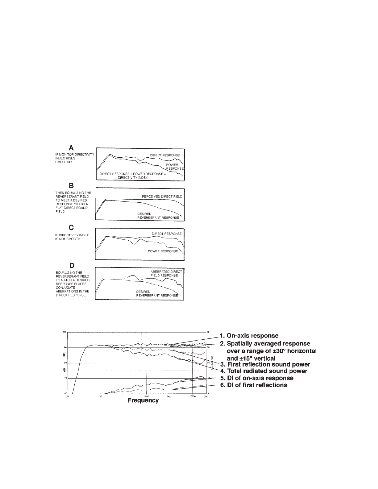
optimum response simultaneously, as
shown at B.

If the loudspeaker has smooth on-axis
response but irregular power response,
as shown at C, then any attempt to
make the reverberant response
uniform will result in irregular on-axis
response – or vice-versa. This is shown
at D (Smith, et al., 1983).

The LSR Principle:

More recently, the desire to extend the
on- off-axis response matching to its
highest degree has led to JBL’s LSR, or

Linear Spatial Reference

monitors. These systems make use of
proper choice of crossover
frequencies, dividing network
adjustments, and specific baffle
boundary details to ensure three very
important performance features:

1. Flat on-axis frequency response.

2. Flat forward listening angle response

(±30° horizontal; ±15° vertical).

3. Uniform, gradually diminishing power
response with rising frequency.

The degree to which the LSR goals
have been met can be summed up in
the single composite graph shown in
Figure 2. Here, we have plotted six
response curves on the LSR6328P
powered monitor:

, series of

Figure 1. The effect of uniform on-axis
response and uniform power response.

Figure 2. Response data for JBL LSR6328P monitor system.

1. Curves 1 and 2 show the forward
only response components. Note that
the averaged response over the
forward listening angle is virtually the
same as the on-axis response.

2

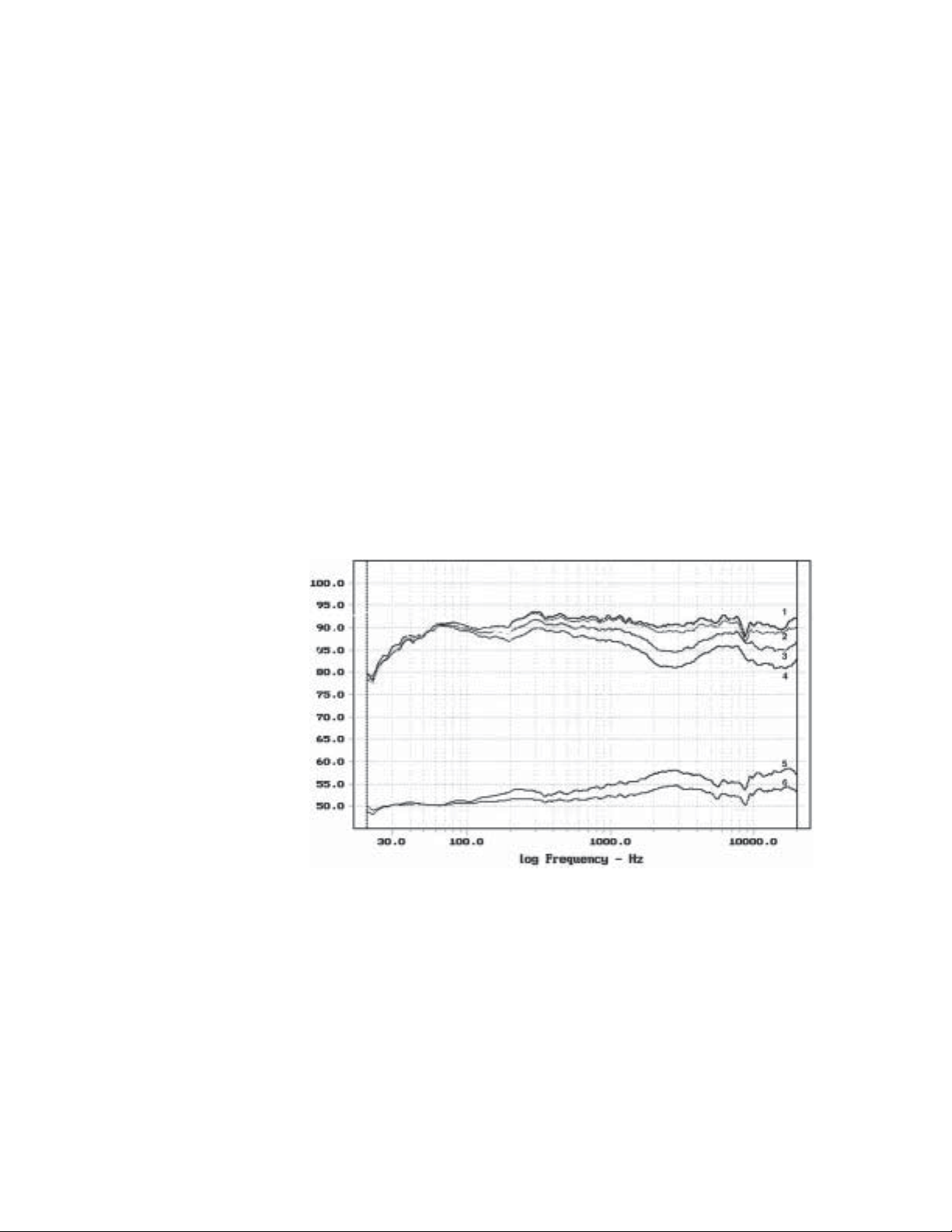
2. Curves 3 and 4 show the radiated
power (power response) of the
system, based on both first reflections
and on total radiated power.

3. Curves 5 and 6 are derived by
subtracting the radiated power curves
from the on-axis curve, giving an
overview of the system’s DI (directivity
index).

Figure 3 shows the same family of
response curves for a competitive
monitor which has not been designed
according to these principles.
Specifically, the power response
(Curves 3 and 4) show significant
peaks and dips in the upper midrange,
which indicate that there will be an
uneven reflected sound field in the
room.

paying for is symmetry of design, bass
traps, and a high degree of acoustical
isolation, all of which may require
extensive structural alterations. The
control room will also likely have large
flush mounted monitors. A room in
your home on the other hand will have
none of these improvements, and
there are two low frequency problems
that you will have to address by non­structural means. One of these has to
do with reflected images of
loudspeakers which are located close
to walls, and the other has to do with
standing waves in the room. We will
now discuss these problems in detail.

Figure 3. Response
data for a sub-optimal
system.

Low Frequency Problems:

Many audio operations are set up in
what we can call “ordinary” rooms. A
spare bedroom is often the choice for
a home workspace, and if it has
carpeting, drapery, bookshelves, and
a few other pieces of furniture, it may
actually be better than you think it is.
When you spend a fortune on a
control room, what you are largely

Boundary Compensation:

JBL’s new powered LSR-series products
incorporate a set of equalizers which
will enable you to make certain low
frequency (LF) adjustments to your
system. The first of these is

Compensation

JBL’s LSR full-range systems are
designed to have flat LF response when

.

Boundary

3

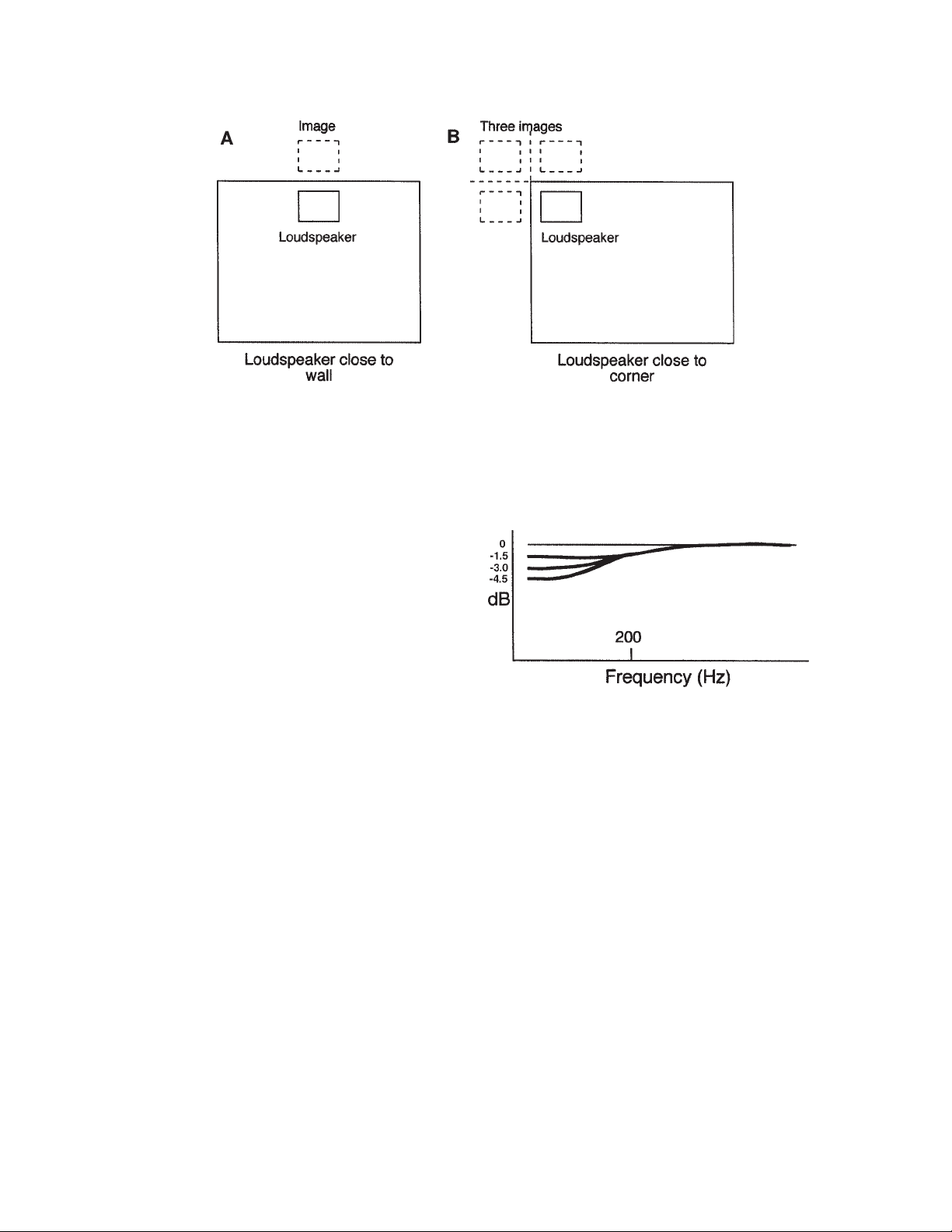
Figure 4. Loudspeaker boundary conditions. Against a wall (A); in a corner (B).

they are mounted on conventional
loudspeaker stands that are normally
placed 2 feet or more from the walls.
When the systems are placed within
about 10 inches of a wall, the
situation will be as shown in Figure 4.
At A, the system is fairly close to a
single wall, and the reflected image of
the loudspeaker will increase the
loudspeaker’s LF loading, resulting in
an increase in output below about 200
Hz. The degree of LF boost will be
approximately 1.5 to 3 dB, depending
on the actual distance from the wall.
Under these conditions, you would
want to
feed to the system by adjusting a set
of DIP switches on the rear panel of
the LSR6328P. The models LSR25P
and LSR6312SP also have boundary
compensating equalization tailored to
their normal mounting alternatives.

Figure 4B shows the effect of posi­tioning the loudspeaker in a corner.
Generally, we don’t recommend this,
but if you are working in a very small
space, such positioning may be
necessary. In this case the maximum
amount of LF cut (4.5 dB) may be
applied. In any event, you will be able
to observe the effects of these
degrees of LF cut as you get further
into the equalization process.

decrease

the amount of LF

Figure 5 shows the range of the
boundary compensation equalizer in
the LSR6328P. Each step is 1.5 dB,
providing a maximum reduction of 4.5
dB below about 200 Hz.

Figure 5. Boundary compensation curves.

Room Modes and RMC (Room
Mode Correction):

Room modes are resonances that
exist between two or more boundaries
of a room. In a rectangular room, the
most common of these are the so-

called axial modes

between opposite walls and between
the floor and ceiling. Figure 6 shows a
side section view of a typical
workspace, and the panel just below
that figure shows the sound pressure
distribution for the first-order axial
mode along the front-back dimension
of the room. The bottom panel shows
the modal pressured distribution for

, which take place

4

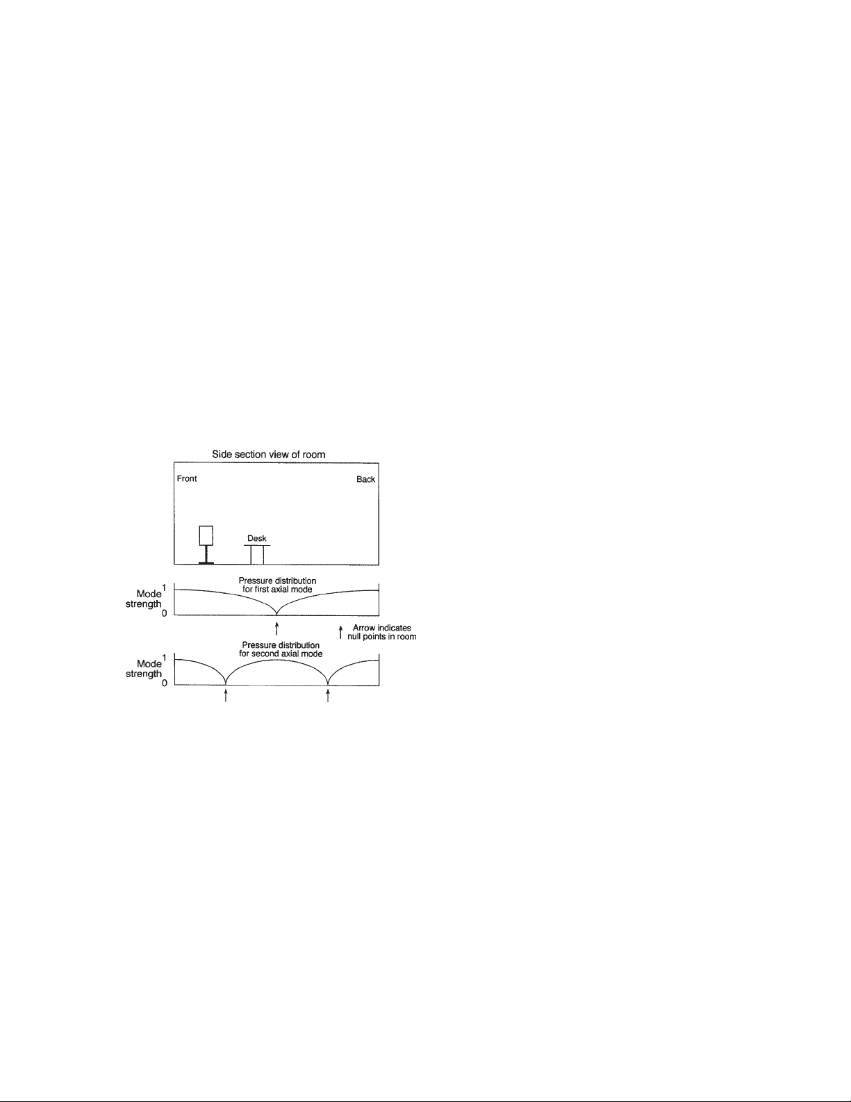
the second-order axial mode, which is
an octave higher than the first.

Let’s assume that the front-back
distance in this space is 20 feet. The
frequency of an axial mode is given by
the following equation:

f = (c/2)(n/l)

where f is the frequency (Hz), c is the
speed of sound (1130 feet/second),
is an integer value (1, 2, 3, etc.), and
is the length of the room in feet.
Solving this for the first-order mode (n
= 1) gives:

f = (1130/2)(1/20) = 28.3 Hz

forth, even slightly, in the null region,
you would hear the 28.3 Hz signal rise
and fall in level – not a good effect!
You will normally want to locate your
listening position clearly out of the null
region.

But let’s consider that you were
constrained, for whatever reason, to
sit directly in the null. As you
continued searching out room modes

n

you would soon run into the first-order

l

axial side-to-side mode and the
second-order front-back axial mode.

Modes are plentiful, and even more
complex modes exist between multiple
room surfaces. But in the normal
course of setting up a room the lowest
axial mode in the longest room
dimension will be the one you will want
to identify and equalize.

Figure 6. Axial modes in a rectangu­lar space.

If we apply a signal at this frequency to
the loudspeaker and walk the room
from front to back, we will hear the LF
signal very loudly at the two ends of
the room, and we will find that it
diminishes considerably in level as we
approach the null region in the middle
of the room.

Assume for a moment that you placed
your work desk right at the null point.
As you moved your head back and

How Does the RMC
Equalization Process Work?

We have gone to great lengths to
simplify the process of identifying
modes and equalizing them. All the
measurement gear that you’ll need is
contained in the RMC kit that
accompanies the model LSR6312SP.
The kit of course can be used to
calibrate and adjust all of your LSR
systems that have RMC capability. The
analysis kit consists of the following
items:

1. Test CD, with noise bands for level
reference and one-tenth octave
warble tones for making frequency
response measurements.

2. A hand-held sound level meter.

3. Chart paper for entering your
measurements.

5

4. A template for measuring the width
(Q) of the response peak.

5. A small tool for making equalizer
settings on the electronics.

6. A comparator switch for making
quick A-B comparisons with and
without RMC.

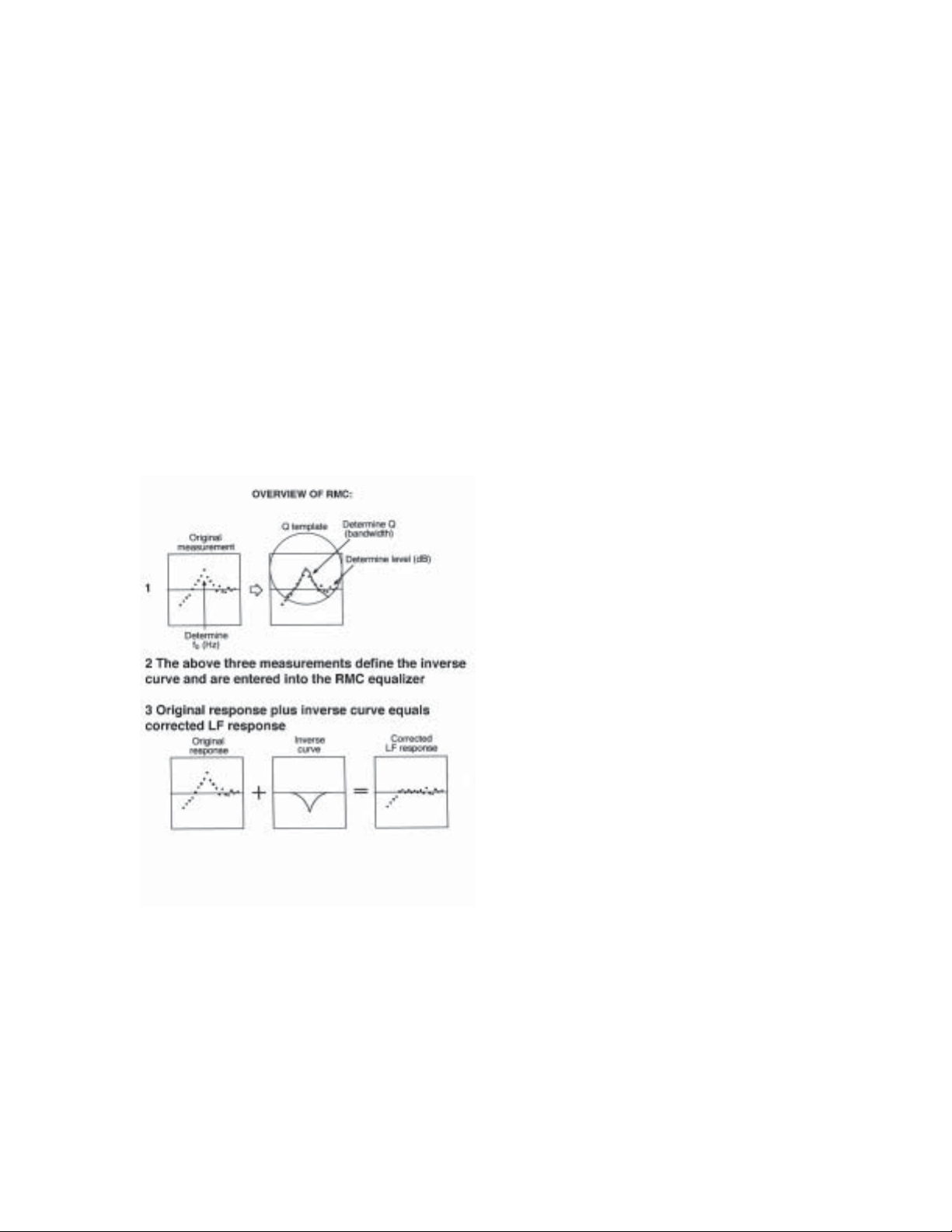
A quick overview of the measurement
process is shown in Figure 7. Using the
test CD, a nominal reference level is
chosen. You then play the sequence of
one-tenth octave warble tones and
manually enter the values on a piece of
chart paper.

You now have the three parametric
values:
These are each entered into the
equalizer on the back of the LSR
electronics via detented
potentiometers. The data you have
entered provides an inverse curve to
the one that you measured, and the
net acoustical response of the
system will be flat over the affected
portion of the frequency range.

At this point you can engage the
equalizer and listen. Or, you can use
the comparator switch box and make
before-after comparisons throughout
the listening space. You may even
wish to fine tune the system purely
by ear.

frequency, width,

and

level

.

Two Typical Examples Using
LSR6328P Systems:

Figure 7. Overview of the RMC process.

Once this has been done, the width
template is placed over the plotted
curve and adjusted so that you get a
good fit between the curve and the
markers on the template. You then
note the width value and the height of
the curve in dB.

Figure 8 shows before and after
measurements in a space where two
peaks were evident in the system’s
response (upper panel). The lower
peak was the one that was
compensated for. It is at 31 Hz and is
7 dB above the established baseline.
Using the width template we arrived
at a width value of 25%. Entering
these values into the parametric
equalizer we arrived at the adjusted
response shown in the lower panel.
You will note that the equalized LF
response between 28 and 105 Hz is

uniform within a range of ±2.5 dB.

The secondary peak at 47 Hz was due
to the first order side-to-side mode in
the listening room.

Figure 9 (upper panel) shows
response with a peak at 41 Hz and a
dip 57 Hz. The dip is caused by a

6

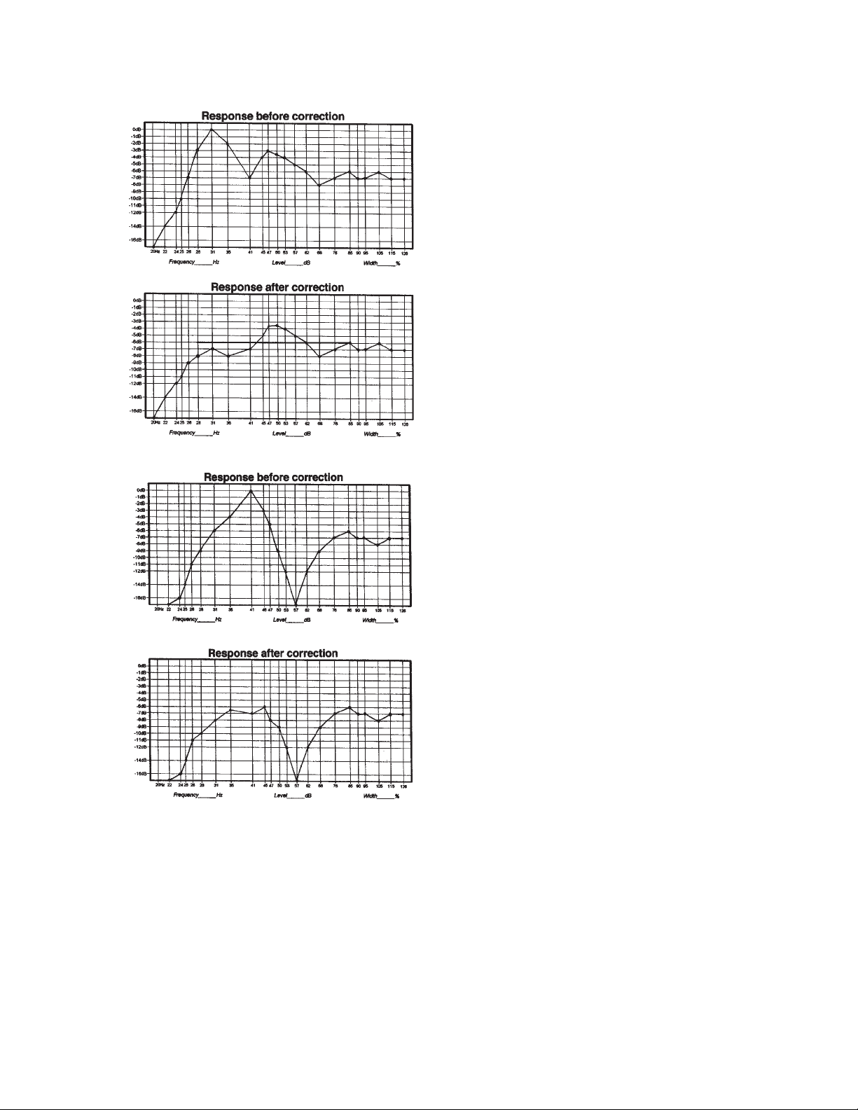
Figure 8. Before-after comparison#1.

little consequence because they are
almost always compensated for by the
response of the subwoofer. The lower
panel of Figure 9 shows the overall
response after the 41 Hz peak has
been reduced by about 7 dB.

A Comparison Between RMC
and One-third Octave
Equalization:

One-third octave EQ is felt by many
engineers to be a cure-all for
loudspeaker-room problems, but this is
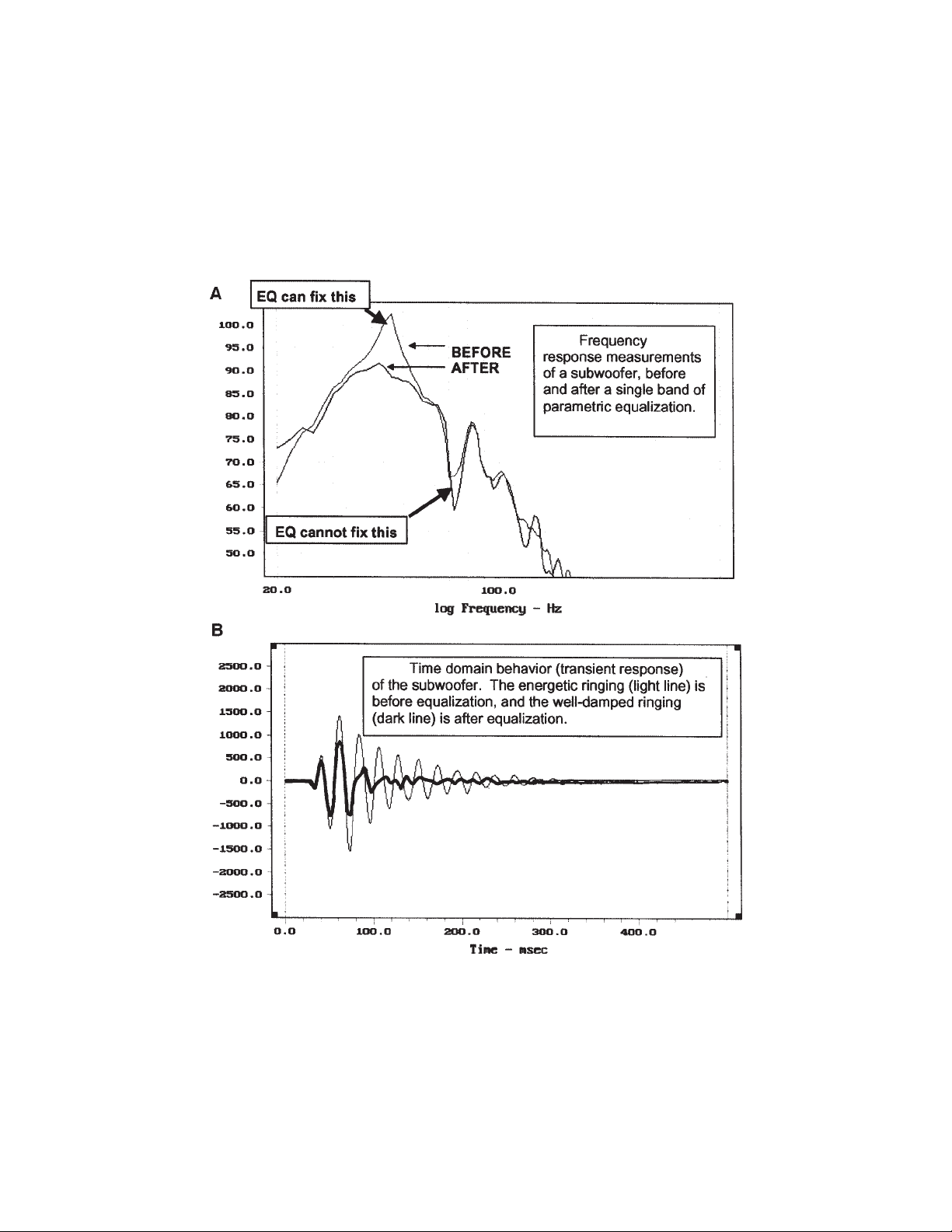
not generally the case. The composite
curve in Figure 10A shows the before
and after MLSSA high resolution
response of a subwoofer exhibiting a
sharp response peak at about 45 Hz.
Note that RMC has reduced the peak
about 14 dB. The effect this has on the
transient response of the system is
shown at B, where it is clear that the
ringing has been heavily damped
(Toole, 2000).

Figure 9. Before-after comparison #2.

floor reflection and cannot be
compensated for with any kind of
equalization. Such dips can usually be
alleviated somewhat by making slight
adjustments in the positions of the
loudspeakers and the listening
locations. Normally, these dips are of

If we had used one-third octave
analysis and equalization to solve this
problem, our analyzer would have
presented us with the data shown in
Figure 11A. There is no indication of
either the sharp 45 Hz peak or the dip
at 70 Hz. In fact, the curve as it exists
doesn’t look all that bad. Using one­third octave filtering, we now EQ the
system to flatten it by about 13 dB, as
shown at B, and it looks even better.

Now, let’s go back and remeasure the
system with MLSSA, as shown in Figure

12. The data at A shows that the sharp
peak is still present, and the ringing,
although somewhat lower in level, has
not been damped out at all.

7

It is obvious that one-third octave
equalization is of no use in damping out
sharp response peaks. It is also a fact
that experienced control room

designers do not normally use one-third
octave equalization for these purposes;
they rely instead on bass traps and
other acoustical damping to remove
such response peaks.

Figure 10. MLSSA measurements of a typical RMC equalization.
Frequency response (A); time domain response (B).

8

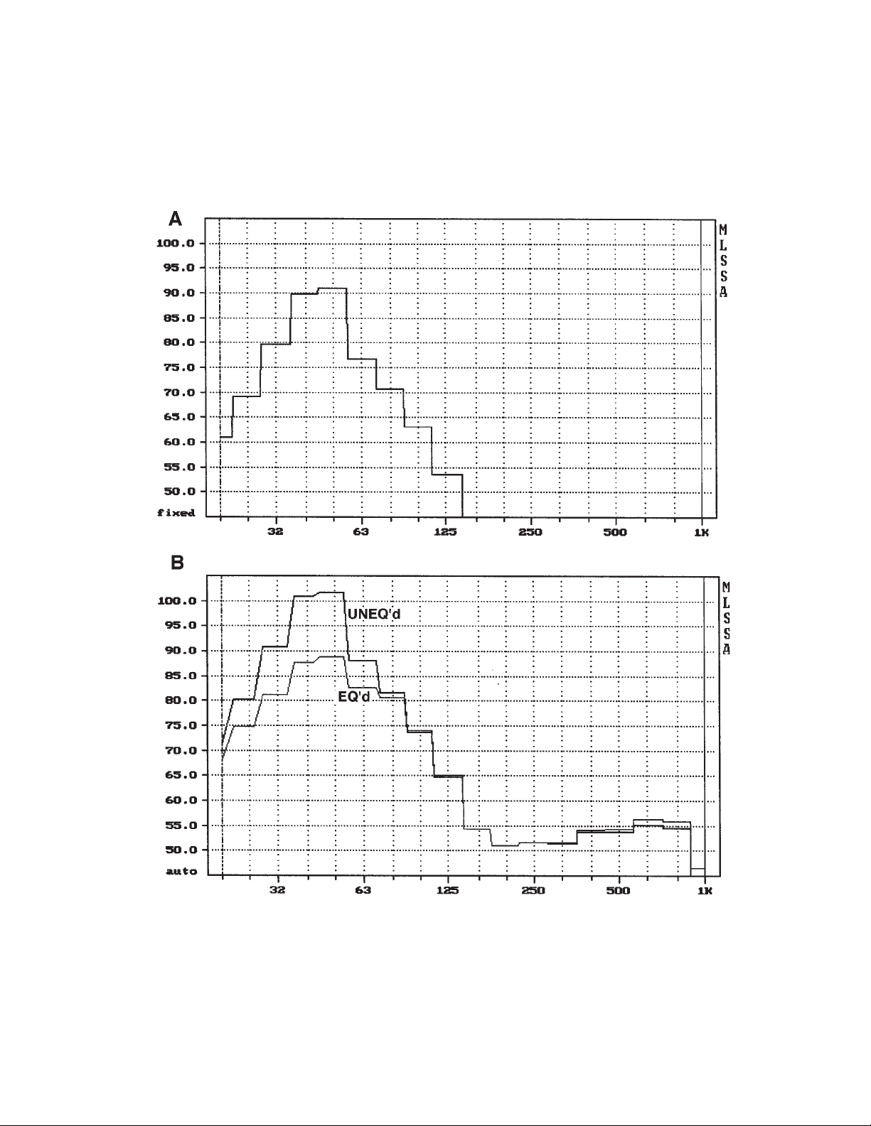
Figure 11. Same setup as before, but viewed with one-third octave analyzer (A);
equalized with one-third octave equalization (B).

9

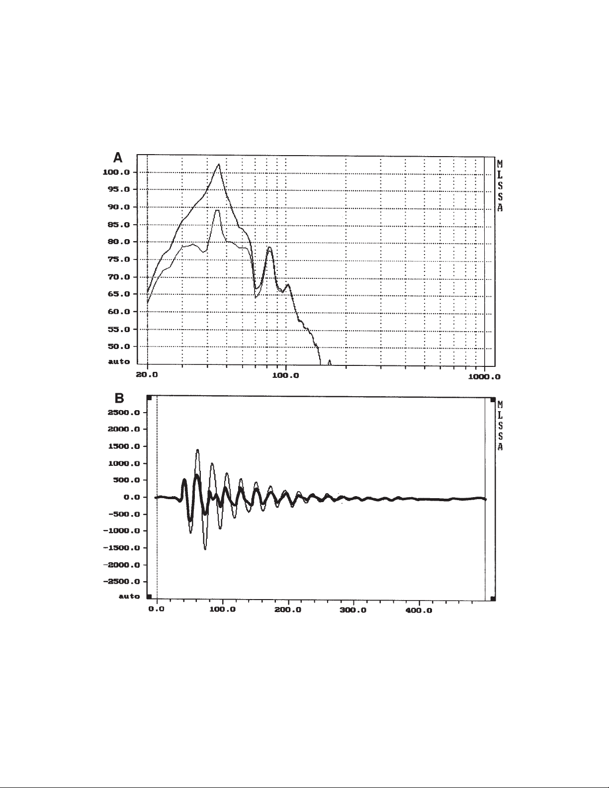
Figure 12. One-third octave equalization viewed with MLSSA (A);
time domain response (B).

10

Conclusions:

RMC is a simple and effective way to ensure smooth LF response in monitoring
spaces that do not have extensive LF acoustical treatment or bass traps. Its
application is intuitively simple and straightforward – and after you have
adjusted any upper bass peaks due to room modes you may be surprised how
low in frequency your recordings actually extend.

You can mix and match systems with and without RMC very easily, For
example, the LSR6312SP subwoofer can be used with the LSR25P, LSR6332,
or any other passive full-range system you choose.

Bibliography and References:

Augspurger, G., “Loudspeakers in Control Rooms and Living Rooms.”
Proceedings of the AES 8th International Conference, Washington, DC (3-6 May

1990).

Cooper, J.,
(1996).

Eargle, J. and Foreman, C.,
Professional, Northridge, CA (2002).

Smith, D., Keele, C. B., and Eargle, J., “Improvements in Monitor Loudspeakers,”
Journal AES, volume 31, number 6 (June 1983).

Toole, F., “Maximizing Loudspeaker Performance in Rooms,” Harman
International White Paper (2000).

“JBL’s New LSR Mid-Field Monitors,” JBL Professional Technical Note, volume 3,
number 2.

“JBL Professional Studio Monitors for Multichannel Sound Applications,” JBL
Professional Technical Note volume 3, number 3.

Building a Recording Studio

Audio Engineering for Sound Reinforcement

, Synergy Group, Inc., Los Angeles

, JBL

11

10/03