

Page 1
Tech Note
TN-0902 Date: 02/06/09
USING A 2CCD CAMERA TO CREATE HIGH-DYNAMIC RANGE IMAGES
Some imaging scenarios push dynamic range beyond the capabilities of the typical sensor. This is especially
true where incident light is present (e.g., imaging a light source and the surrounding area). This can also
occur in situations with bright reections or in high contrast indoor/outdoor scenes where one needs to capture details in both bright sunlight and dark shadows. One technique for dealing with these situations is to
combine or “fuse” two images with different exposures so that the dynamic range is signicantly increased.
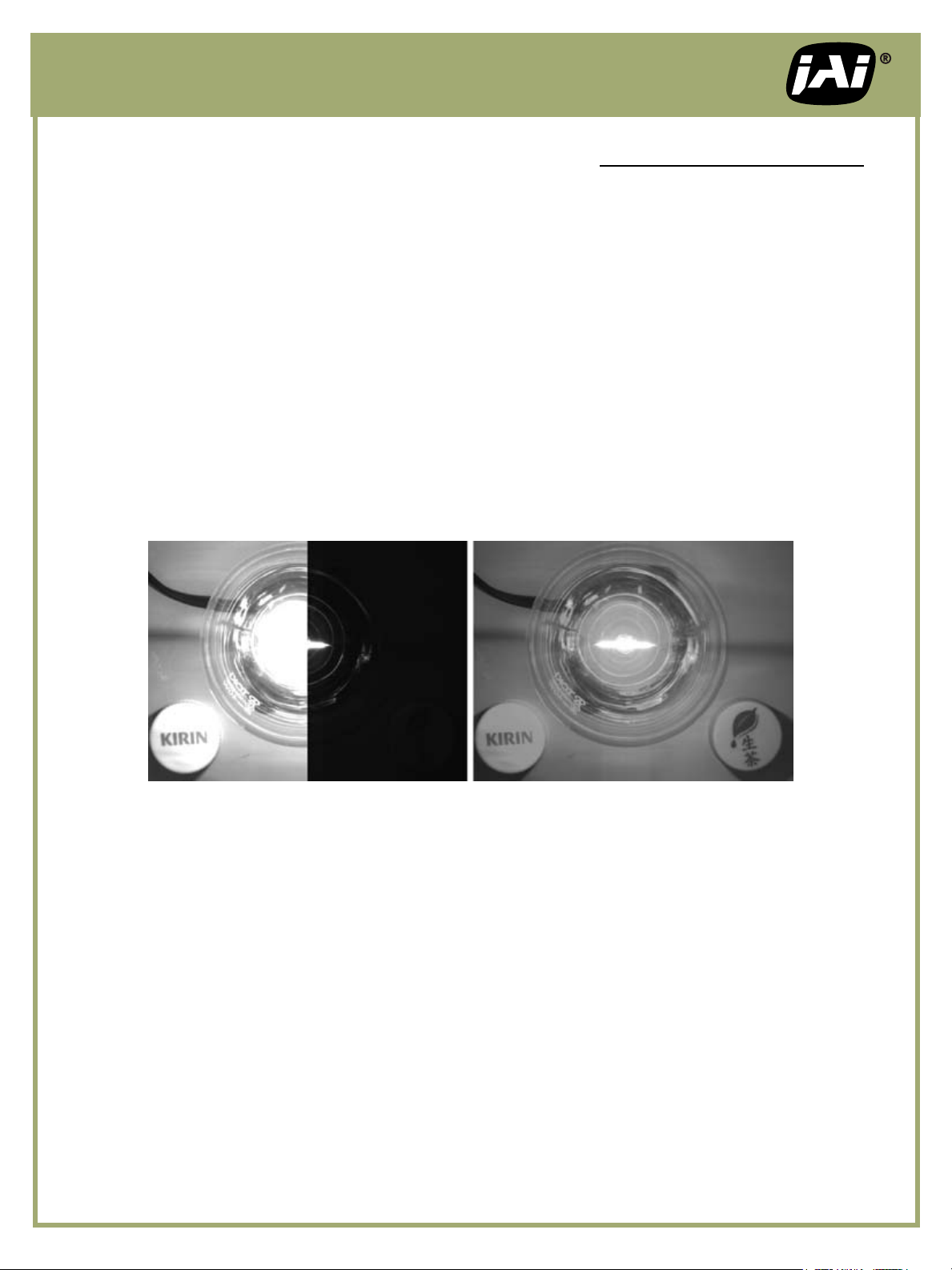
An illustration of this technique can be seen in the following images captured by JAI’s AD-081 camera. Here,
the incident light coming from the light bulb makes it impossible to examine both the bright and the dark
areas of this scene in a single exposure. Instead, two exposures are used as shown in Figure 1. The left half
of the image shows what the image looks like when captured with a slow shutter speed. This is able to
capture details in the surrounding areas while letting the brightest parts of the scene over saturate. The
right half of the image shows the result of a much faster shutter speed, enabling details to be seen in the
brightest portions of the image while rendering much of the surrounding area as nearly black. When “fused,”
as shown in Figure 2, the composite image is able to span the full dynamic range of the scene.
FIGURE 1 – Bracketing the exposure FIGURE 2 – Fused HDR image
In landscape or architectural photography, this effect be achieved with a single CCD camera taking two
consecutive images. However, in “live action” settings – such as industrial inspections, surveillance, vehicle
applications, and the like – the presence of motion requires simultaneous capture of the two images that are
to be fused. This can be done with two cameras, looking at the same scene. However, to avoid alignment issues, it is best if the CCDs are in a single camera with a prism-based 2CCD arrangement. The AD-081 camera
from JAI uses this 2CCD prism-based approach to increase dynamic range while ensuring precise registration
of the two image streams.
Note: in some industrial settings, it may be possible to use a one-camera scenario if the object being in-
spected stops briey and the camera being used has the ability to automatically take two closely-spaced images with dramatically different gain and/or shutter settings. JAI’s “sequence trigger” function supports this
approach, where feasible. It is available in many of the company’s C3 Camera Suite models with GigE Vision
interfaces.
Calibrating sensor response and output
In a 2CCD scenario such as the AD-081CL, establishing a high dynamic range image comes from fusing the
output of the two sensors to effectively increase the bit depth of the nal image. The mathematical equation for the display then becomes a function of the calibration of the 2 sensors. There are several strategies
that can be used.
Page 2
Tech Note
Example 1 - Maximum Dynamic Range (no overlap)
To create an image that spans the maximum range of light intensities, use shutter settings to calibrate the 2
sensors so that Sensor B = Sensor A * 1024. In other words, the light needed to generate 100 counts from Sensor B is 1024 times the light needed to create 100 counts from Sensor A.
For example, if Sensor A is operating with the shutter off (1/30 sec.), Sensor B would need to be set as close
as possible to 1/30720 sec. using the camera’s pre-set shutter or programmable exposure control. This would
result in 1 count of output from Sensor B being roughly equivalent to what would be 1024 counts from Sensor
A, had it not saturated at 1023 counts.
Now, create a fused image by applying a post processing routine that uses output from Sensor A when it is
below saturation and from Sensor B when Sensor A is saturated. A simplied representation of this routine
could be the Boolean expression:
if (pixel B < 1){
pixel_out = pixel A
}else{
pixel_out = pixel B * 1024
}
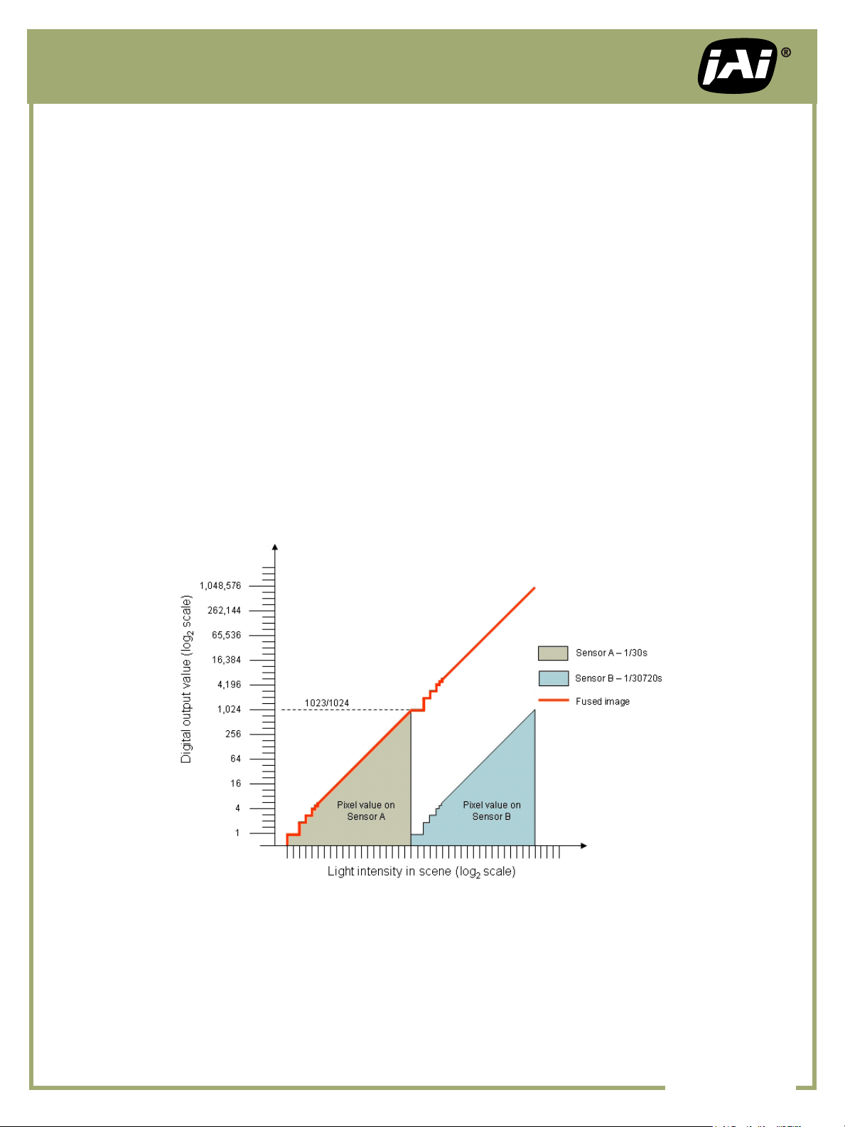
This approach uses Sensor B to add 10 more bits of dynamic range to the image, albeit at a lower precision
than the lower 10-bits due to the calibration factor (see Figure 3). Creating the actual algorithm for fusing
the two images will depend on the type of post processing software being used. It could involve writing programming code, or could be done in a more visual fashion using a graphical user interface.
FIGURE 3 – Maximum dynamic range calibration
One issue with any high dynamic range approach is that it is hard to display or print such an image. Besides
the challenge of handling the data in a Microsoft OS, most displays and/or printers do not have this much
dynamic range and will diminish your good work. Typical computer monitors today feature contrast ratios
on the order of 1,000 to 1, enabling them to approximate 10-bit dynamic range (~60 dB). A growing number
of monitors today offer contrast ratios in the 2,000:1 to 5,000:1 range enabling them to support 12 bits of
dynamic range (~72 dB).
NO. TN-0902 pg 2
2
Page 3

Tech Note
Displaying a high dynamic range image on a standard monitor will require mapping the output to t the
monitor’s dynamic range capability. For the image described above, start by creating a 20-bit image map
using the raw pixel data. Then create a 10-bit image map to display on the monitor by dividing the 20-bit image map by 1024. Or create a 12-bit image map by dividing the 20-bit image map by 512.
The preceding process describes using both output channels in 10-bit mode. Alternatively you can use the
8-bit output from both channels to create a 16-bit HDR image. To do this, use the same method as described
above, only calibrate the 2 sensors so that Sensor B = Sensor A * 256. This reduces the total dynamic range,
but increases the precision of output values in the upper half of the range.
Example 2 - Overlapping Dynamic Range
Example 1 provides the maximum dynamic range possible using 10-bit output. However, there may be issues
around the 1023/1024 count transition that cause problems in the fused image. This is because of the fast
shutter speed being used on Sensor B and the relatively low output precision (i.e., 1 count = 1024 while 2
counts = 2048). This means that the inherent noise in Sensor B has a much more noticeable effect, causing some pixels that are very close in actual light intensity to be output with dramatically different values.
While this type of impact is expected in the darkest portions of an image, its effect on luminance values
around the transition point can result in some very noticeable artifacts.
One approach for mitigating this phenomenon is to overlap the responses of the two sensors by 2-4 bits. This
reduces the total dynamic range, but also signicantly reduces the amplication of noise at the transition
point to provide a better overall image throughout the full range.
For example, to produce a cleaner transition in a 16-bit image, calibrate the sensors using the process described in Example 1 (using 10-bits per channel output), but make the transition point 64 counts, so Sensor B
= Sensor A * 64. Now the 4 MSB of Sensor A will overlap with the 4 LSB of Sensor B (see Figure 4).
FIGURE 4 – Overlapping sensor calibration
NO. TN-0902 pg 3
2
Page 4

Tech Note
Now, our post processing routine could be handled as follows:
if (pixel B < 16){
pixel_out = pixel A
}else{
pixel_out = pixel B * 64
}
By overlapping the two sensor responses, this approach utilizes the full precision of the lower 10-bits while
reducing the effect of noise at the transition point and greatly increasing the precision of the upper 6-bits.
Example 3 – Averaging the Overlap
Both of the preceding examples assume that a precise calibration can be made between the two sensors,
resulting in a linear output (when plotted on a logarithmic scale). In reality, even the AD-081’s programmable
exposure capability, which allows shutter speed to be adjusted in one-line increments (42.07 µs), will still
not provide the precision needed for perfect calibration.
As a result, if the methods described in Examples 1 or 2 are used, this will produce a sharp discontinuity in
the output response line at the transition point between the two sensors (see Figure 5).
FIGURE 5 – Sensor B calibration off by 1 count (64 counts in output)
This transition can be “smoothed” by averaging the values of Sensor A and Sensor B in the area of the graph
leading up to the transition point. For example, using the same calibration point as described in Example 2,
we could create a Boolean expression where the output value of the 16-bit image uses the average of the
two sensors’ response in the region of the last overlapped bit. For example:
if (pixel A < 512){
pixel_out = pixel A
}elseif (pixel B < 16){
pixel_out = (pixel A + (pixel B * 64))/2
}else{
pixel_out = pixel B * 64
}
NO. TN-0902 pg 4
2
Page 5

Tech Note
Now as Sensor A approaches its saturation point (512 – 1023 counts) the output uses the average of both sensors’ data to “smooth” the transition between the two sensor response graphs (see Figure 6). It still limits
the use of the lowest bits on Sensor B (those that are most susceptible to noise) and keeps the calibration
factor at 64 to increase the output precision of the upper bits.
FIGURE 6 – Averaging used to smooth calibration in overlapped region
Example 4 – Dual-Slope Dynamic Range
Lastly, you can use the approach described in Example 3 to smooth the transition between two sensor output
lines that have intentionally been given different slopes. This dual-slope arrangement can be used to compress or expand the dynamic range in a particular region of the luminance values -- similar to a look-up
table, but over an expanded dynamic range as shown in Figure 7.
To use this approach, overlap and calibrate the two sensor responses as in Example 2, as if a post-processing
factor of 64 was going to be applied to the value of Sensor B. However, during post processing, apply a
smaller multiplier for Sensor B, combined with a specic offset value, to create a “atter” output line that
intersects the output from Sensor A somewhere in the uppermost bit of its output graph.
FIGURE 7 – Dual-slope HDR calibration
NO. TN-0902 pg 5
2
Page 6

Tech Note
For example, in a 4-bit overlap scenario, we still set the shutter for Sensor B to be roughly 64 times faster
than Sensor A (i.e., a pixel on Sensor A with a value of 256 would have a value of 4 on Sensor B). But, depending on our objective, we apply a post processing factor of less than 64 and add an offset value to get
the two output graphs to intersect somewhere around 768 counts.
Finally, use a post processing algorithm that averages the values of Sensor A and B in the last bit as illustrated in Example 3. This will create a smooth transition region to merge the slopes of the two output graphs.
The sample algorithm below uses a multiplier of 4 and an offset of 720 to produce a dual-slope graph that
compresses the upper 6 bits of light intensity received (64,512 counts) into the 2 upper bits of the image
output (~3,000 counts) for a 12-bit image that spans 16-bits of dynamic range.
if (pixel A < 512){
pixel_out = pixel A
}elseif (pixel B < 16){
pixel_out = (pixel A + ((pixel B * 4)+720))/2
}else{
pixel_out = (pixel B * 4) + 720
}
By applying a variety of different equations to this dual-slope concept, users can utilize the two sensors to
accommodate many different lighting scenarios. This might include attening the slope of Sensor A while
increasing the slope of Sensor B, or using complex math to create an “S” curve in the nal output.
In all of the previous examples, the shutter speed was used to calibrate the two sensors. It is also possible to
use gain for calibration or a combination of shutter and gain to get as close as possible to precise calibration.
Be aware, however, that increasing gain will also impact the noise level of the sensor output, which may or
may not be acceptable for a particular application.
For more information about high dynamic range imaging or the AD-081 camera, please contact JAI.
NO. TN-0902 pg 6
2
 Loading...