

Page 1

D-0105222 - E - 2017/09
Additional Information
Eclipse
Valid from software version:
EPx5 4.5
ASSR 1.2.7
ABRIS 1.06.2
DPOAE 1.03.2
TEOAE 3.04.3
Page 2

Page 3

Table of contents
1 Launching the software.................................................................................................................... 1
1.1 Starting up from OtoAccessTM ............................................................................................... 1
1.1.1 Module Setup in OtoAccess ™ .................................................................................. 1
1.2 Starting up from NOAH (ASSR only)..................................................................................... 2
1.3 Change & view License ......................................................................................................... 3
Ensuring the Eclipse is working properly ......................................................................................... 5
2
2.1 Calibration of Eclipse ............................................................................................................. 5
2.1.1 peSPL to nHL correction values ............................................................................... 6
2.2 Limiting noise in the test environment ................................................................................... 7
2.2.1 Grounding ................................................................................................................. 7
2.2.2 The best Test Site & Setup for ABR recordings ....................................................... 7
2.2.3 Limiting noise - Equipment setup ............................................................................. 8
2.2.4 Limiting noise - During testing .................................................................................. 9
2.2.5 Changing protocol settings to limit electrical interference ........................................ 9
2.2.6 Determination of noise during a recording ............................................................... 9
2.3 Service check using the Loop back box (LBK15) ................................................................ 10
2.4 Testing noise level on the artificial patient LBK15 ............................................................... 12
2.4.1 Check the amplitudes of the EEG with LBK15 ....................................................... 13
EP15/25 ......................................................................................................................................... 15
3
3.1 About EP15/25 Module ....................................................................................................... 15
3.2 Brief Introduction to ABR ..................................................................................................... 16
3.3 The EP15/25 Menu Items .................................................................................................... 17
3.4 General Operation of EP 15/25 ........................................................................................... 18
3.4.1 Toolbar .................................................................................................................... 18
3.4.2 Record tab .............................................................................................................. 20
3.4.3 Rejection level ........................................................................................................ 21
3.4.3.1 Advanced Rejection ................................................................................ 22
3.4.4 Fmp and Residual Noise ........................................................................................ 23
3.4.5 Graph area .............................................................................................................. 25
3.4.5.1 Changing the Gain and Time scale ......................................................... 25
3.4.5.2 Right click in the graph area .................................................................... 25
3.4.5.3 Right click on the curve handle ............................................................... 26
3.5 Edit tab ................................................................................................................................ 29
3.5.1 Assigning Waveform Markers and Labels .............................................................. 29
3.5.1.1 Latency times .......................................................................................... 31
3.5.2 Double Cursor / measuring individual differences .................................................. 32
3.5.3 Filter settings .......................................................................................................... 32
3.5.4 Show Condition / show Fmp Graph ........................................................................ 33
3.5.5 Latency Template ................................................................................................... 33
3.6 Latency tab .......................................................................................................................... 34
3.7 System Setup ...................................................................................................................... 36
3.7.1 Auto Protocols ........................................................................................................ 36
3.7.1.1 Predefined protocol settings .................................................................... 36
3.7.1.2 Type of measurement ............................................................................. 37
3.7.1.3 Print Wizard ............................................................................................. 37
3.7.1.4 Stimulus properties ................................................................................. 37
3.7.1.5 Filter properties ....................................................................................... 41
3.7.1.6 Display properties ................................................................................... 45
3.7.1.7 Recording properties ............................................................................... 46
3.7.1.8 Recording begin and end ........................................................................ 47
3.7.1.9 Rejection ................................................................................................. 47
Page 4

3.7.1.10
3.7.1.11 Wave Reproducibility (Wave repro) ........................................................ 50
3.7.1.12 Research availability (only with research licence) .................................. 50
3.7.1.13 Special tests ............................................................................................ 50
3.7.2 General Setup ......................................................................................................... 51
3.7.2.1 External Trigger Output ........................................................................... 51
3.7.2.2 Auto Protocol Options (Separating ears) ................................................ 51
3.7.2.3 Language ................................................................................................ 52
3.7.2.4 ECochG Area Function ........................................................................... 52
3.7.2.5 Quick stimulus rate .................................................................................. 52
3.7.2.6 Special Waveform Markers ..................................................................... 53
3.7.2.7 Display Options ....................................................................................... 53
3.7.2.8 Level measure method ............................................................................ 55
3.7.2.9 Export Waveform .................................................................................... 55
3.7.3 Latency Template ................................................................................................... 56
3.7.4 Report Templates ................................................................................................... 58
3.8 Printing ................................................................................................................................ 59
3.8.1 Print options from file menu .................................................................................... 59
3.8.2 Printer Setup ........................................................................................................... 61
3.8.3 Print Wizard ............................................................................................................ 61
3.9 Preparation Prior to Testing ................................................................................................ 64
3.9.1 Instruction of the patient ......................................................................................... 64
3.9.2 Visual inspection of the ear canal ........................................................................... 64
3.9.3 Preparation of the Skin ........................................................................................... 64
3.9.4 Placement of Electrodes ......................................................................................... 65
3.10 Impedance Check................................................................................................................ 66
3.10.1 Insertion of eartips .................................................................................................. 66
3.10.2 Placement of bone conductor ................................................................................. 67
3.11 ABR Masking ....................................................................................................................... 67
3.12 ABR Threshold Determination ............................................................................................. 68
3.12.1 Protocol Settings for Threshold Determination ....................................................... 68
3.12.2 ABR Threshold Results .......................................................................................... 69
3.12.3 Protocol Settings for Bone Conduction ABR .......................................................... 70
3.13 Neuro Latency Examination ................................................................................................ 71
3.13.1 Protocol Settings for Neuro Latency Examination .................................................. 71
3.14 Neuro Rate Study Examination ........................................................................................... 72
3.14.1 Protocol Settings for Neuro Rate Study Examination............................................. 72
3.15 eABR – Trigger Enabled (if included in your license) .......................................................... 73
3.15.1 Protocol Settings for eABR ..................................................................................... 73
3.15.2 Using the Eclipse Trigger ....................................................................................... 74
3.16 ECochG (Electrochochleargraphy) (if included in your license) .......................................... 76
3.16.1 Protocol Settings for ECochG ................................................................................. 76
3.17 Cochlear Microphonic (CM) (if included in your license) ..................................................... 77
3.17.1 Protocol settings for CM ......................................................................................... 77
3.18 AMLR (if included in your license) ....................................................................................... 78
3.18.1 Protocol settings for AMLR ..................................................................................... 78
3.19 ALR (if included in your license) .......................................................................................... 79
3.19.1 Protocol settings for ALR ........................................................................................ 79
3.20 P300 (if included in your license) ........................................................................................ 80
3.20.1 Protocol settings for P300 (if included in your license)........................................... 80
3.21 MMN (if included in your license) ........................................................................................ 81
3.21.1 Protocol settings for MMN ...................................................................................... 81
3.22 Loop Back ............................................................................................................................ 82
3.23 EP 15/EP25 PC shortcuts ................................................................................................... 83
Research Module ........................................................................................................................... 85
4
4.1 Logging data (while recording) ............................................................................................ 85
4.2 Exporting the single curve ................................................................................................... 86
Optimized recording ................................................................................ 48
Page 5

Exporting the whole session ................................................................................................ 86
4.3
4.4 Exporting waveform when of f line ........................................................................................ 87
4.5 Exporting data from another laptop ..................................................................................... 87
4.6 Exporting other data ............................................................................................................ 87
4.7 Technical details of the research module ............................................................................ 88
4.8 Import of XML-file in external program ................................................................................ 89
4.8.1 Import in Excel ........................................................................................................ 89
4.8.2 Import in Notepad ++ (freeware), Microsoft notepad or Internet Explorer .............. 92
4.9 A practical demonstration of export: .................................................................................... 92
4.10 Has the insert tubing time delay been compensated? ........................................................ 95
4.11 How to import WAV files for stimuli ..................................................................................... 96
4.12 Da, Ba & Ga wavefile sounds .............................................................................................. 99
4.13 Extracting all sessions for selected patient. ........................................................................ 99
VEMP ........................................................................................................................................... 103
5
5.1 About the VEMP module ................................................................................................... 103
5.2 The VEMP Menu Items ..................................................................................................... 103
5.3 General Operation of VEMP .............................................................................................. 104
5.3.1 Edit Tab ................................................................................................................ 106
5.4 System setup ..................................................................................................................... 111
5.5 General Setup - VEMP ...................................................................................................... 114
5.6 Protocol settings cVEMP ................................................................................................... 115
5.7 Preparing for the cVEMP ................................................................................................... 116
5.7.1 Visual inspection of the ear canal ......................................................................... 116
5.7.2 Preparation of the skin .......................................................................................... 116
5.7.3 Electrode placement ............................................................................................. 116
5.7.4 Impedance check button ...................................................................................... 117
5.7.5 Test procedure and Instruction of Patient ............................................................ 117
5.7.6 Insertion of foam ear tips ...................................................................................... 117
5.8 Performing a cVEMP measurement .................................................................................. 118
5.9 cVEMP Results .................................................................................................................. 119
5.10 Protocol settings oVEMP ................................................................................................... 121
5.11 Preparing for the oVEMP .................................................................................................. 122
5.11.1 Visual inspection of the ear canal ......................................................................... 122
5.11.2 Preparation of the skin .......................................................................................... 122
5.11.3 Electrode placement ............................................................................................. 122
5.11.4 Impedance check button ...................................................................................... 123
5.11.5 Test procedure and Instruction of Patient ............................................................ 123
5.11.6 Insertion of eartips ................................................................................................ 123
5.12 Performing an oVEMP measurement ................................................................................ 124
5.13 oVEMP Results ................................................................................................................. 125
ASSR ........................................................................................................................................... 127
6
6.1 About the ASSR module ................................................................................................... 127
6.2 Brief Introduction to ASSR ................................................................................................ 127
6.2.1 Analysis ................................................................................................................ 127
6.2.2 NB CE-Chirp® for ASSR ...................................................................................... 128
6.2.3 SNR in ASSR ........................................................................................................ 129
6.3 The ASSR Menu Items ...................................................................................................... 130
6.4 General operation of ASSR ............................................................................................... 131
6.4.1 Toolbar .................................................................................................................. 131
6.4.2 The ASSR tab ....................................................................................................... 133
6.4.2.1 The left panel user interface .................................................................. 133
6.4.2.2 EEG ....................................................................................................... 134
6.4.2.3 Frequency Curves ................................................................................. 134
6.4.2.4 Right clicking on a handle ..................................................................... 135
6.4.2.5 The Table .............................................................................................. 136
6.4.3 The Audiogram tab ............................................................................................... 137
Page 6

6.4.3.1
6.5 System setup ..................................................................................................................... 139
6.5.1 Auto Tests Setup .................................................................................................. 139
6.5.2 General Setup ....................................................................................................... 141
6.5.3 Report Templates ................................................................................................. 142
6.5.4 Correction Factors ................................................................................................ 143
6.5.4.1 Correction factor values ........................................................................ 143
6.6 Preparing for an ASSR measurement ............................................................................... 145
6.6.1 Visual inspection of the ear canal ......................................................................... 145
6.6.2 Instruction of patient ............................................................................................. 145
6.6.3 Preparation of skin ................................................................................................ 145
6.6.4 Electrode placement ............................................................................................. 146
6.6.5 Insertion of the Eartips .......................................................................................... 146
6.6.6 Impedance check.................................................................................................. 146
6.7 Performing an ASSR ......................................................................................................... 148
Starting ASSR from OtoAccess™ or NOAH ..................................................................... 148
Performing an ASSR measurement .................................................................................. 148
6.8 ASSR Results .................................................................................................................... 149
6.9 BC ASSR ........................................................................................................................... 151
6.9.1 Incorrect detection by transducer induced ElectroMagnetic Interference (EMI) .. 151
6.9.2 Placement of bone conductor ............................................................................... 152
6.10 ASSR Masking .................................................................................................................. 153
6.11 NOAH Compatibility........................................................................................................... 155
6.12 ASSR PC shortcuts ........................................................................................................... 155
ABRIS .......................................................................................................................................... 157
7
7.1 About the ABRIS module .................................................................................................. 157
7.2 The ABRIS Menu Items ..................................................................................................... 157
7.3 General Operation of ABRIS ............................................................................................. 158
7.4 System setup ..................................................................................................................... 160
7.4.1 General Setup ....................................................................................................... 160
7.4.2 Report Setup ......................................................................................................... 161
7.4.3 Password .............................................................................................................. 162
7.5 Preparing for a ABRIS measurement ................................................................................ 163
7.5.1 Visual inspection of the ear canal ......................................................................... 163
7.5.2 Instruction of patient ............................................................................................. 163
7.5.3 Preparation of skin ................................................................................................ 163
7.5.4 Placement of Electrodes ....................................................................................... 163
7.5.5 Impedance Check ................................................................................................. 164
7.6 Performing a ABRIS measurement ................................................................................... 164
7.7 ABRIS Results ................................................................................................................... 165
7.8 ABRIS PC shortcuts .......................................................................................................... 166
DPOAE ........................................................................................................................................ 167
8
8.1 About the DPOAE module ................................................................................................. 167
8.1.1 Brief Introduction to DPOAE ................................................................................. 167
8.2 The DPOAE Menu Items ................................................................................................... 168
8.3 General Operation of DPOAE20 ....................................................................................... 169
8.4 DPOAE20 System Setup .................................................................................................. 173
8.4.1 Auto Test Setup .................................................................................................... 173
8.4.2 Template ............................................................................................................... 174
8.4.3 Norm Data ............................................................................................................ 175
8.5 Preparing for a DPOAE measurement .............................................................................. 176
8.5.1 Visual inspection of the ear canal ......................................................................... 176
8.5.2 Instruction of patient ............................................................................................. 176
8.5.3 Probe selection ..................................................................................................... 176
8.6 Performing a DPOAE measurement ................................................................................. 177
8.7 Results ............................................................................................................................... 178
Correction factors in Estimated Audiogram .......................................... 137
Page 7

DPOAE PC shortcuts ........................................................................................................ 182
8.8
TEOAE ......................................................................................................................................... 183
9
9.1 About the TEOAE25 module ............................................................................................. 183
9.2 Brief Introduction to TEOAE .............................................................................................. 183
9.3 The TEOAE25 Menu Items ............................................................................................... 184
9.4 General Operation of TEOAE25 ........................................................................................ 185
9.5 TEOAE25 System Setup ................................................................................................... 187
9.5.1 Auto Test .............................................................................................................. 187
9.5.2 General Setup ....................................................................................................... 189
9.5.3 Printer Layout ....................................................................................................... 190
9.5.4 Report Templates ................................................................................................. 191
9.5.5 Auto Screening ..................................................................................................... 192
9.6 Preparing for a TEAOE measurement .............................................................................. 193
9.6.1 Visual inspection of the ear canal ......................................................................... 193
9.6.2 Instruction of patient ............................................................................................. 193
9.6.3 Probe selection ..................................................................................................... 193
9.7 Performing a TEAOE measurement.................................................................................. 194
9.7.1 Probe Check ......................................................................................................... 194
9.7.2 Rejection level ...................................................................................................... 194
9.7.3 Start the test ......................................................................................................... 194
9.7.4 TEOAE Results..................................................................................................... 195
9.8 TEOAE PC shortcuts ......................................................................................................... 197
FAQ & Trouble Shooting.............................................................................................................. 199
10
10.1 General FAQ ..................................................................................................................... 199
10.2 FAQ – ABR ........................................................................................................................ 204
10.2.1 ABR preparation ................................................................................................... 204
10.2.2 ABR Recordings ................................................................................................... 204
10.2.3 ABR user interface................................................................................................ 207
10.2.4 ABR Latency data ................................................................................................. 208
10.2.5 ABR Disposables & Accessories .......................................................................... 209
10.2.6 ABR System ......................................................................................................... 210
10.3 FAQ – VEMP ..................................................................................................................... 211
10.4 FAQ – ASSR ..................................................................................................................... 212
10.5 FAQ – DPOAE ................................................................................................................... 215
Dictionary ..................................................................................................................................... 217
11
References & Relevant articles ................................................................................................... 223
12
Page 8

Page 9

Throughout this manual the following meaning of warnings, cautions and notices are used:
WARNING indicates a hazardous situation which, if not avoided, could result in death or serious injury.
CAUTION, used with the safety alert symbol, indicates a hazardous situation which, if not avoided, could result in minor or moderate injury.
NOTICE NOTICE is used to address practices not related to personal injury.
Page 10

Page 11

Eclipse Additional Information Page 1
1 Launching the software
1.1 Starting up from OtoAccessTM
Ensure that the Eclipse is on, before performing recordings and then open the software module. If the hardware is not detected the selected Eclipse module can still be opened in reader mode.
When the system is in reader station mode, it is not possible do any recordings. However, it is still possible to
examine, filter and label all recordings .
To start from OtoAcce ss™:
1. Open OtoAccess™
2. Select the patient you want to work with by highlighting it blue.
3. If the patient is not yet listed:
press the New client button
fill in at least the mandatory fields, marked with a red asterisk.
save the patient details by pressing the Save patient information button.
4. Select Instrument will show the modules you have for your Eclipse. EP15/25, ASSR, DPOAE, TEOAE,
and ABRIS are modules related to the Eclipse. Double click on the module to start the test.
1.1.1 Module Setup in OtoAccess™
If the software module icon does not appear in the Select Instrument box in OtoAccess™:
1. Go to File | Setup | Instruments tab
2. Create a new instrument, by:
a. Type in the Software module name in the New Instrument name field
b. Select the relevant module from the Software modules dropdown menu
c. Select Eclipse from the Hardware dropdown menu
d. Select USB connection
e. Press Create
f. Press Apply Settings
g. Press OK to exit
Page 12

Eclipse Additional Information Page 2
.
For further instructions about working with the database, please see the operation manual for OtoAccess™.
1.2 Starting up from NOAH (ASSR only)
1. Open NOAH
2. Select the patient you want to work with by highlighting it orange
3. If the patient is not yet listed:
press the Add a New Patient button
fill in the required fields
save the patient details by pressing the OK button.
4. Double click on the ASSR module.
For further instructions about working with the NOAH database, please see the operation manual for NOAH.
Page 13

Eclipse Additional Information Page 3
1.3 Change & view License
The License keys of the Eclipse ar e specif ic f or each s erial number and define which modules and tests
functionalities are available.
As a user you always have the opportunity to upgrade your software to a newer version. The License is
found under Help | About for all module on the Eclipse.
If for instance you want to upgrade from EP15 to EP25, this can be done by a change of the license key
number written in the dialog box About. Interacoustics A/S has to get the serial number from the customer in
order to create a new license key.
The Eclipse serial number is located on the backside of the Eclipse. Alternatively the DSP serial number
01.003.230 can be used.
This license key is stored in Eclipse, as well as in the Interacoustics manufacturing database, so that we can
find the license key already stored in the box, even if the customer gives us only the serial no of the DSP
board mentioned above.
When pressing the license button you open the License Manager. In this dialog box it is possible to enter the
new license key. When the dialog box comes up, the old license key is already marked, so that it is possible
to press Ctrl+C and then paste this string into an email, in order to send the old license key to us.
When you receive the ne w Licens e number from your manufactur e enter/copy it in the field New License
Key. When entered press OK.
Note In the License Manager, it is only possible to press OK, if a valid license key is entered. Therefore it is
not possible for you as a user to enter an invalid license key and this way make the system un-useable.
Page 14
Eclipse Additional Information Page 4
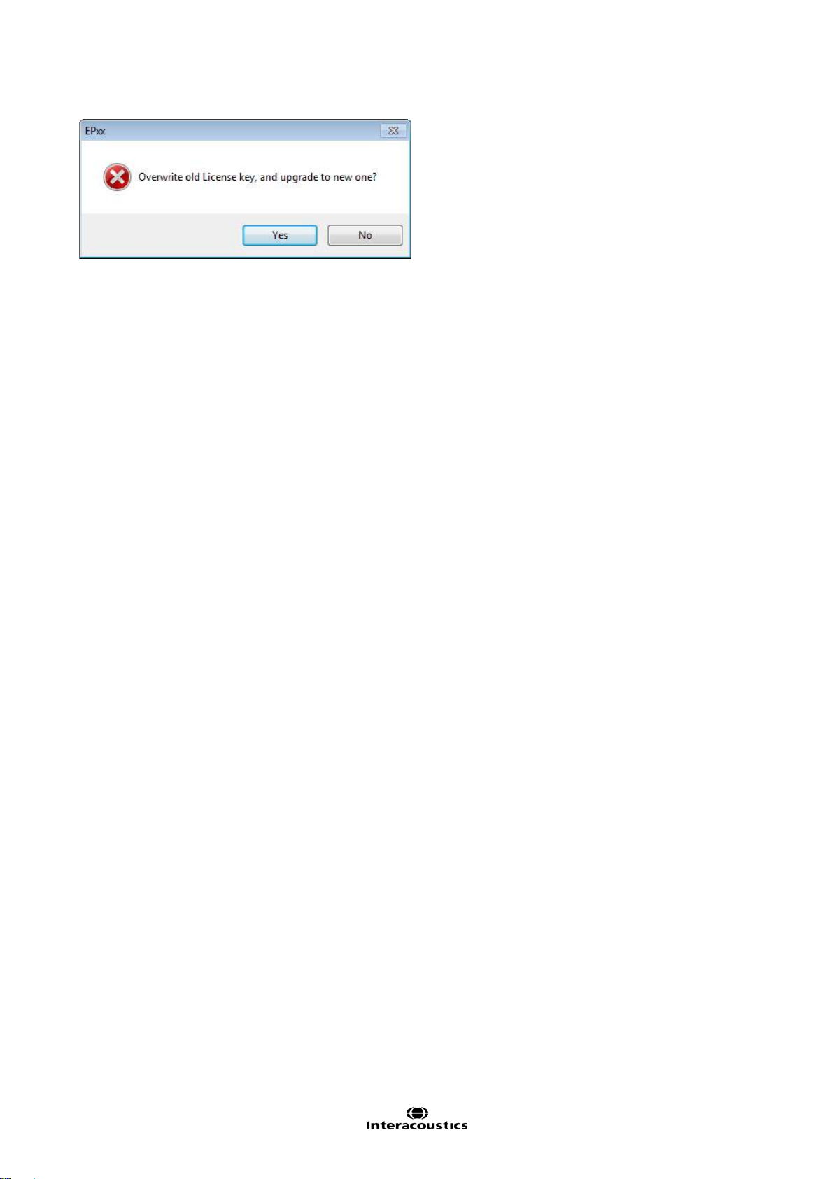
When pressing OK the program asks to store the new license key. Press Yes to overwrite the old License
key. The application has to be restarted in order to activate the new features.
Page 15

Eclipse Additional Information Page 5
2 Ensuring the Eclipse is working properly
2.1 Calibration of Eclipse
It is recommended that an Interacoustics distributor calibrate the instrument once a year.
Two types of calibration are used in the world of AEP – peSPL (peak equivalent Sound Pressure Level) and
nHL (normal Hearing Level).
peSPL is an objective measure of the sound stimulus pressure level. For a given peSPL dB value, the max
acoustical or vibration level is calibrated to match the level of continuous tones used to obtain the same
dBSPL reading on a sound level meter. As the duration of sound stimuli for AEP are extremely short, the energy delivered is not perceived with the same subjective loudness as the equivalent stimulus would provide,
if it were a continuous tone. Therefore the acoustical or vibration value given in dB peSPL does not correspond very well with normal HL figures. For Clicks there is a 35.5dB difference (70dBpeSPL sounds as
35dBHL), and for Tone Bursts the differences are in the 20-30dB range depending on frequency and number
of sine waves used in burst.
Stimulus intensity is limited to 135.5dBpeSPL by the transducers.
nHL is a correction, which c om pens ates for the difference in perceived loudness of the very brief stimuli like
Clicks and tone bursts. There is therefore a direct similarity between the indicated level in nHL and the HL
levels well known from normal audiometry. Brief tone burst correction values from peSPL to nHL are based
on a 2-1-2 manual burst as specified in ISO 389-6-2007. Longer duration tone bursts for AMLR and ALR are
employing peRETSPL values similar to continuous pure tones (as used in conventional audiometers) since
the temporal integration of tones lasting at least 50ms is considered sufficiently trivial to ignore.
Note Reference calibration values for the CE-Chirp® stimulus family are not specified in the current interna-
tional calibration standard (ISO 389-6), and the applied peRETSPL values have therefore been derived from
two studies: (1) by PTB in Germany (2008), and (2) by DTU in Denmark (Gøtsche-Rasmussen et al., 2012).
The mean of the values obtained in the two studies, rounded to the nearest 0.5 dB, are used by Interacoustics A/S to calibrate the broad-band CE Chirp® LS and the four frequency specific NB CE-Chirp® LSs delivered by the ER-3A earphone.
The following tables give the reference equivalent thresholds for various stimuli in dB peSPL and dB peVFL
Note The RETSPL figures given for ABR 3A inserts are for measurements made in an occluded ear simulator (IEC 60318-4 / 60711) not a 2cc / HA-2 coupler, for which different values apply. Unofficial figures for the
HA-2 coupler are available at: http://hearing.screening.nhs.uk/calibration
Remember to check Eclipse stimuli levels. An easy sound check with the transducer left on the table
is often a good manual weekly procedure.
.
Page 16

Eclipse Additional Information Page 6
Toneburst
Toneburst
Hz
Insert Phone
Headphone
Bone
Hz
Insert Phone
Headphone
Bone
250
28
32
74.5
250
17.5
27
67
500
23.5
23
69.5
500
9.5
13.5
58
750
21
19
61
750 6 9
48.5
1000
21.5
18.5
56
1000
5.5
7.5
42.5
1500
26
21
51,5
1500
9.5
7.5
36.5
2000
28.5
25
47.5
2000
11.5
9
31
3000
30
25.5
46
3000
13
11.5
30
4000
32.5
27.5
52
4000
15
12
35.5
ISO 389-6:2007
ISO 389-1:2000, ISO 389-2:1994, ISO 389-3:1994
Click
Click
Insert Phone
Headphone
Bone
Insert Phone
Headphone
Bone
Click
35.5
31
51.5
Click
35.5
31
51.5
NB CE-Chirp® LS
NB CE-Chirp® LS
Hz
Insert Phone
Headphone
Bone
Hz
Insert Phone
Headphone
Bone
500
25.5
25
74
500
25.5
25
74
1000
24.0
21.0
61.0
1000
24.0
21.0
61.0
2000
30.5
27
50
2000
30.5
27
50
4000
34.5
29.5
55.0
4000
34.5
29.5
55.0
CE-Chirp® LS
CE-Chirp® LS
Insert Phone
Headphone
Bone
Insert Phone
Headphone
Bone
31.5
27.0
51.0 31.5
27.0
51.0
2.1.1 peSPL to nHL correction values
ECochG/ABR15/ABR30/AMLR/Neuro/VE MP 0 dB 2-1-2 cycle
linear envelope
ECochG/ABR15/ABR30/AMLR/Neuro/VEMP 0 dB
ALR/MMN 0 dB 25-50-25 ms
ALR/MMN 0 dB
ECochG/ABR15/ABR30/AMLR/Neuro/VEMP 0 dB
ECochG/ABR15/ABR30/AMLR/Neuro/VEMP 0 dB
ALR/MMN 0 dB
ALR/MMN 0 dB
Only toneburst correction values change for ALR & MMN testing.
For Click and CE-Chirps
Maximum stimulus intensity is limited to 100dBnHL by the air conduction transducers.
The ABR unit leaves the factory with nHL calibration, but it can easily be changed to peSPL values. Please
refer to the FAQ or contact your local Interacoustics distributor if you are interested in changing the calibration unit.
®
LS, the same correction is applied.
Page 17
Eclipse Additional Information Page 7
2.2 Limiting noise in the test environment
The smallest ABR signals are in the size of 100-150nV clos e to thresho ld, so it can be difficult to obtain a
good SNR.
Proper grounding is essenti al in order to obtain a response with a minimum of electrical noise.
Try to ensure:
1. A dedicated ground for the Eclipse will reduce noise, please consult with the chapter Grounding.
2. Electrical interference must be minimize in order to get the best ABR waves for threshold estimation;
please turn off other equipment’s not used or move them further away from patient.
3. Always connect the patient bed/chair to the Eclipse ground outlet; this will reduce electrical noise further.
4. An electrical shielded room can be used to avoid electrical noisy from the environment.
2.2.1 Grounding
Grounding is crucial for cleaner ABR waves and safe operation. The ABR system cabinet is connected to the
ground lead. If the ground lead is not connected or poor, the ABR system will pick up electrical noise/interference. This is on the screen as very large harmonic distortion curves completely overlaying the ABR curves.
An electrician can often easily wire a separate ground to the power outlet and swap the ground in this
socket. The time/money the electrician spends is much worth when it comes to the saved time for less noisy
ABR measurements.
Due to High Voltage, only experienced technicians/ properly trained staff must change and check the ground. Typically
an electrician has a dedicated ground tester where they can measure the quality of the ground.
Do not connect the Eclipse to a safety transformer, as a safety transformer is built in to the Eclipse already.
When ensuring grounding be aware of the following:
1. We must instruct the electrician that w e are tr ying to rec ord ABR signals as tiny as 100nV, as most of
them will determine that their ground is good enough for the house. Yes is might be good enough for
laptops, PC’s or televisions – BUT NOT for ABR!
2. It is highly recommended to use a separate ground, as other equipment in the building can easily pollute the ground (discharging current, spikes and noise to the ground).
3. There should be maximum 8 ohm between the earth rods to the place where ground is used with the
Eclipse.
2.2.2 The best Test Si te & Setup for ABR recordings
1. If Laptop/PC is connected to power outlet – an optical USB cable must be used in order to maintain
patient safety (optical cable available).
2. An electric magnetic shielded room – typically soundproof.
3. Dedicated separated ground for only the ABR recording site.
4. The bed framing may act as an antenna. Ground it to the backside of the Eclipse and turn of the
power when connecting the cable . In worst case replace the bed with a wooden/plastic chair bed
and check whether the metal bed was the reason for noise.
Page 18

Eclipse Additional Information Page 8
5. Always disconnect any powering of the patient bed during ABR test. It will cause more noise. We
have several cases where the noise was more than halved after the patient bed was disconnected to
power. A bed with a battery can cause noise even when the bed is not plugged into the wall, and
should be replaced with a bed without a battery.
6. Try to move the test site within the room; patient might be close to a power cord etc. perhaps hidden
in the wall close to patient and electrodes.
7. Position patient/child with head towards center of the room, not the wall, especially if there is a power
source at the head of the bed.
8. Request a quiet room, preferably away from roads, rooms containing power supplies/fuse boards.
9. Do not position equipment near mains sockets.
10. The test room should be placed away from devices causing electrical interference (e.g. autoclaves,
microwave ovens, mobile phones, hospital pager systems, lifts, escalators, air conditioning systems,
etc.).
11. Li ght and other electrical equipment not being used should be turned off as the patient will work as
an antenna and pick up electrical interferences.
12. Remember to turn off all other electrical equipment not used in the room, especially sources with
neon lights.
13. Do not use light dimming switches (a notorious source of interference).
14. E lectrical interference may also appear through the ground lead if this is interconnected to many
computers, autoclaves, instruments using high power etc.
15. Unplug any non-essential networked computers in the room, remembering to remove the network
cable from the data socket located on the wall. Make the patient lay down to reduce interference
from neck muscle contractions.
16. For babies be prepared to suggest alternative positions, e.g. for the baby to be placed in a car seat,
rather than being held by a parent.
17. In some cases, it may be necessary to find another test location if there is too much ambient acousti-
cal or electrical noise.
Operating rooms
1. Operating rooms are usually acoustically noisy. Insert earphones help attenuate ambient acoustic
noise and are safer in post-myringotomy cases where blood could make an electrical connection between the patient and the transducer, but the transducer should be held (with a drip stand) at a
higher level than the tip to avoid blood entering the transducer under gravity.
2. Pulse oximeters are sometimes the source of electrical interference. Try turning it off to see if this
eliminates the interference (if so, then neg oti ate w it h the anaesthetist to do without if possible). If an
oximeter is used, position as far away from patient and equipment as possible (at patient’s feet end).
Even if the oximeter is run on battery it may create interference.
3. Sedation pumps (mostly running on batteries) should at any time be positioned as far as possible
away from the patient electrodes.
4. If many types of equipment are connected to the patient, use the same power outlet to minimize the
small current leakage through patient.
2.2.3 Limiting noise - Equipment setup
1. Always check the wall outlet for a proper ground when establishing an ABR test room. Sometimes
the ground lead is found inside the wall outlet, but is not connected to ground.
2. Carry out listening check if no responses are seen or unusual waveforms are recorded.
3. Odd-looking responses can be recorded if the electrode leads are incorrectly connected (response
may be inverted) and a flat-line is likely if we inadverte ntly record across the mastoids.
4. If interference occurs try running the laptop on battery, disconnected from its power supply and with
the power supply unplugged (check battery charge is adequate to complete the test).
5. Do not cross over any leads or cabling, especi al ly elec trode, tr ans duc er, and power supply leads.
Page 19

Eclipse Additional Information Page 9
2.2.4 Limiting noise - During testing
1. Run electrode cable from one direction to the patient and earphone tubes or cables from the other
direction to the patient – do not let them cross.
2. Run electrode leads close together or better braid the electrodes leads.
3. It is a common mistake to place the active electrode too low and the mastoid electrode too high.
4. The preamplifier electrode “ground” lead can be used to address noise.
5. Ex. Patient is connected to a pulse oxygen meter left arm, or ECG heart monitor move the ground to
left shoulder. Noise is now lead first to the ground and the driven right leg preamplifier which will reduce the electrical noise on the Vertex, R/L leads.
6. When the patient is connected noise levels can differ more, relative to when measuring the noise
level without the patient connected. Therefore, it is important to check the noise levels without the
patient connected to the system by using the LBK15 artificial patient.
7. Adjust the rejection on screen. The most appropriate input rejection level on screen is equal to or less
than 40uV. Typically ABR recordings should be made with an input gain level of 40uV. The lower the
rejection the more sensitive the system. The rejection level should be increased until the real time
EEG signal is not red and rejected.
lowest gain possible, without rejection.
8. Make sure that your electrodes are mounted correctly by checking the impedance.
9. Instruct the patient to be relaxed and calm – a sleeping patient can deliver good ABR/ASSR/ABRIS
results. Eyes should be closed. Please refer to the section “Prep ar ati on Prior t o Tes ting” for a detailed description of a good ABR procedure including instruction of the patient and placement of electrodes.
The higher the gain the more noise is recorded, always use the
Note It’s important to have the same test conditions and parameters in each test when comparing results.
2.2.5 Changing protocol settings to limit electrical interference
In the ABR module go to File | System setup | Auto Protocols setup tab to check how different elements
(filter settings, stimulus rate), which may help you optimize your ABR recordings.
Increase the high pass filter from 33Hz to 100Hz 12/oct.
Choose another stimulus rate ex. 11.1 stim/sec to allow better neural syn-
chronization.
If repeatable noise is recorded, use the feature Minimize Interference.
Please note using a filter setting like this may reduce the amplitude in the ABR waveforms and degrade the
accuracy of hearing threshold measurement tests. However it may be needed if it is impossible to obtain
ABR curves without excessive electrical interference e.g. 50Hz.
2.2.6 Determination of noise during a recording
Before starting a measure with stimuli it can be beneficial to check the amount of noise.
Therefore it is beneficial to have a reference where you start measuring with the electrodes m ounted on patient and the insert phones placed in the ear canal but with the tube of the insert phones clamped.
That will provide you with a baseline of all recorded information collected when no sound is present. The optimal recordings for right and left respectively are then two flat lines indicating that picked up noise is averaged out.
Page 20

Eclipse Additional Information Page 10
2.3 Service check using the Loop back box (LBK15)
The ABR system can be tested using the loop back box LBK15. The test can be used to check the recording
and stimulating circuits of the Eclipse and the Preamplifier with attached cables.
Note that the LBK test can only be used for testing the EP15/25 system and is not valid for functional testing
of the ASSR and ABRIS detection algorithms.
1. Testing the electrical stimuli and recording path
Connect the loop back box to the pre-amplifier using the cabl e with electr o de butt o ns and connec t the
LBK15 jack plug to the right (red) or left (blue) headset channel on the Eclipse.
2. Start the EPx5 software and select the LoopBack - LBK15 from the protocol list.
3. Check the Preamplifier impedance circuit. Choose Impedance mode (IMP) setting on LBK15 and Preamplifier and turn the impedance knob on the pre-amplifier to around 3kOhm. The LED´s must change from
red to green when the impedances on the artificial patient (LBK15) are below 3kOhm.
If it does not turn green around 3kOhm, it can indicate a broken electrode cable or preamplifier cable. Exchange the broken part.
While Impedance mode is enabled the EEG will indicate full rejection on the screen.
Press the Imp button on the preamplifier again when finished to turn off Impedance mode.
4. You should be able to perform the test with an input gain of +/- 40µV. The EEG curve should be black before you start the test. Repeat the test on the other channel if both must be tested.
Note If the EEG curve is red it can indicate no/poor ground is connected to the Eclipse or you have to
search for noise sources (see the section “Limiting noise in the test environment” to help you locate the
noise source).
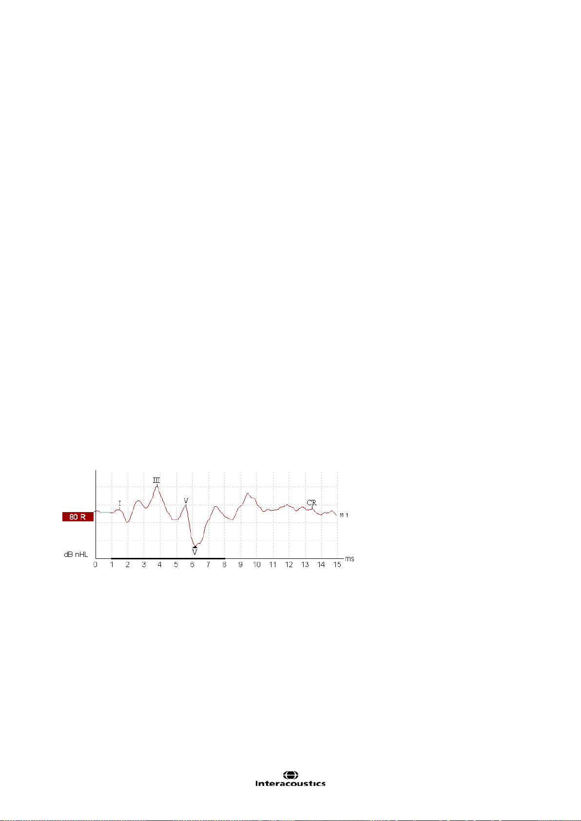
5. To check the signal output, start the test. The evoked potential for right and left with an output at 80dB
should be similar (in fact they are never 100% similar as the individual calibrated transducers are not connected), see picture example below. If one is much smaller/bigger than the other there might be a problem with the pre-amplifier or output stage to the transducers in the Eclipse, perform a listening check of
the transducers to check if the output are similar.
An intensity deviation can be adjusted with a software calibration (see the service manual for calibration
guidance).
Page 21

Eclipse Additional Information Page 11
6. You have now tested the system with the stimulus Tone Burst of 2kHz, to verify that the hardware functions properly.
7. To change the test frequency, select the wanted frequency from the drop down menu on the toolbar.
8. If you want to test with a different stimulus (e.g. click), you can press the icon Setup to make a temporary
change of the loop back test. The output of the LBK with a click is shown below.
9. Press start to start the test. The recording beg ins at -2ms because the default transducer is insert
phones. Due to the latency in the insert earphones, the sound must travel through the silicone tubes and
into the ear, the stimuli is presented at -0.9ms before recording at time 0ms in order to compensate for
the insert phones delay. If you use the headphones the stimuli is fired at 0.1ms as there is a minor delay.
NOTE As a supplement to the Loop Back test it is of good procedure to perform an easy sound check to ensure an equal output from the left and right transducer.
Page 22

Eclipse Additional Information Page 12
2.4 Testing noise level on the artificial patient LBK15
This test is using the default included LBK test box. The red LBK15 stimuli 6.3mm plug is not connected to
the Eclipse stimuli socket.
The red 6.3mm plug is placed non-connected to anything on the table/patient bed.
The electrode cables are connected to the nipples on the LBK15 unit, see picture below.
This way we can simulate a sleeping deaf neonate.
1. If no ground is connected, you will see full rejection on the EEG display in the ABR module, check that
there is ground in the wall outlet as well the power cord.
2. Be careful to place the Eclips e too close EMI radiation sources, especially transf ormers.
3. Do not touch the system or patient bed as you can ground the chassis, and in this way lead to different
results. Often better recordings are seen, not reflecting the patient test scenario, where the operator cannot touch the part during testing.
4. Optimally test with the LBK and Eclipse on same position as you would place the test subjects.
5. Check that electrode fall off is working as expected, full rejection is expected when one lead is disconnected (example of check of left electrode is shown below).
If one cable is broken, change firstly the cable/electrode with the highest impedance and recheck if more
need to be swapped.
6. Check that the impedances are around 3kOhm with the LBK switch in IMP setting.
Page 23

Eclipse Additional Information Page 13
2.4.1 Check the amplitudes of the EEG with LBK15
Double click on the EEG to get picture belo w.
Use and move the horizontal curtains in the EEG box to read the peak to peak amplitude of the EEG. Typi-
cally an amplitude of 2uV peak to peak is expected for electrical quit surroundings.
You can also troubleshoot which part makes noise while monitoring the EEG while moving the potential
noisy parts.
1. Select Threshold Click (included to all licenses) or the protocol you want to check out.
2. The Threshold Click uses a filtering of 1500-33Hz.
3. Uncheck the residual noise stop criteria to let the test run for a longer time (the Threshold Click protocol
will stop the test when the residual noise is down to 40nV which often is after 800 sweeps in this test).
4. Select intensity, if using higher intensities > 80dB nHL take account for EMI from transducers.
5. Start the recording and analyze the results obtained.
Typically a residual noise of 16nV is expected after 4000 sweeps for electrical quit surroundings.
Note The LBK15 is an electrical circuit and will not mimic a patient 100% as human tissue interacts differently to electrical noise compared to a passive electrical circuit with 4 resistors (LBK15).
The LBK15 testing noise levels can be used as a good guideline for troubleshooting but indeed also for practicing the test protocols before a test subject is connected.
Page 24

Eclipse Additional Information Page 14
Page 25

Eclipse Additional Information Page 15
3 EP15/25
3.1 About EP15/25 Module
The Eclipse EP15 and EP25 are intended for use in the electrophysiological evaluation, documentation and
diagnosis of ear disorders in humans. EP15/EP25 is a 2 channel evoked potential system that allows for recording waveforms that can be used for screening and diagnostic applications.
The EP15 allows for the recording of ABRs (Auditory Brainstem Responses) while the EP25 allows for recording ABRs, middle and late latenc y potenti als . The target pop ul ati on for EP15 and EP 25 incl udes all
ages.
The EP 15/25 unit is capable of recording a variety of auditory evoked potentials, but because of its popularity and importance, the auditory brainstem response (ABR) is used as the primary example of EP15/25 use
and in the terminology describing more general applications. The data acquisition of the ABR recordings
takes place from the surface electrodes mounted at specific recording points on the patient.
The analogue ABR recordings are amplified in the external Preamplifier connected to the electrodes. The
amplified analogue ABR recordings are converted into a digital signal in the ADC (Analog to Digital Converter) inside the Eclipse. The digital ABR recordings undergo data processing handled by the PC to improve
the ABR recordings. The ABR-recordings are displayed on the monitor for the operator for further examination and diagnosis. All ABR recordings are stored on the laptop or desktop computer hard drive for later examination and diagnosis.
The EP15/EP25 module contains the following default protocols where VEM P is described in a separate
chapter.
NOTICE
Protocols not included by your license are not visible when the Eclipse is connected.
Page 26
Eclipse Additional Information Page 16
3.2 Brief Introduction to ABR
When a well-functioning ear is stimulated with sound electrical activities are generated within the cochlea as
well as in the combined nerve system connecting the cochlea to the brain. The cortex itself also generates
electrical activities when a sound is processed at these high levels of brain activity.
All of these electrical activities spread to a certain degree through the surrounding tissue and are therefore
also present, though at a very low level, on the outer surface of the head, at the earlobe, within the ear canal,
etc. The electrical potential generated by the brainstem as a result of sound stimulation is around 100nV
upto 1µV when measured in the far field (on the surface of the head), and picked up by electrodes placed in
relevant locations on the head or in the ear canal.
Unfortunately many other electrical activities are present on the surface of the head. These originate from
brain activity, muscle activity etc. Such activities generate electrical potentials at the head normally around
20µV. The largest contributor to this is muscle activity.
When we need to record the AEP (Auditory Evoked Potentials), we are facing the problem of the very poor
signal to noise ratio explained above. The solution is simple in theory, and it is based on the fact that the
noise is random in character, while the AEP signal follows the same exact pattern every time a given sound
is presented to the ear. During testing the sound stimulus is presented to the ear many times, each time followed by a recording of the AEP in a time window starting at stimulus onset and running for a certain number
of milliseconds. Remember that this signal contains two parts: 1) a very small signal stemming from the
nerve activity related to the sound stimulation, and 2) a much larger signal from muscles and unre lat ed br ain
activity which for the purposes of our test we regard as electrical noise. All the recordings are then simply
added together and their average value is calculated at each point in the time window. What will be the average then at any given point? Well, let us look at the noise part of the signal first.
Remember that the noise was random in character, so chances are that there will be as many negative electrical values as there will be positive electr ica l values . And here comes the point: When averaged the positive values will tend to cancel out the negative values. This is why often several thousand stimuli are presented, so we can get thousands of samples to contribute to this averaging process to make the noise disappear. But what about the signal content we are looking for - the AEP?
Luckily, that is the same every time we stimulated with our sound stimulus. Imagine after 6ms from stimulus
onset, you have the presence of the signal albeit at a very low level. As the high level noise has disappears
due to our averaging process described above, we will now be able to see this very small ABR signal.
Example of the auditory brainstem response (ABR) neuro testing:
Remember that it is a recording of electrical nerve activity resulting from a sound stimulus. It is therefore not
a test of hearing in the traditional sense.
As transmission time through the nervous system is well known, it is possible to concentrate on various
points in time relative to stimulus onset. The longer the time window, the deeper can we look into the brain.
Please refer to the quick guides to see and read more about the various AEP tests.
Page 27

Eclipse Additional Information Page 17
3.3 The EP15/25 Menu Items
From the main menu, the following options are available - Setup, Print, Edit or Help. The menu has the following structure:
File | Setup System allows you to enter the EP15/25 setup w here the setti ngs of all protoc ols can be viewed
and changed.
File | Print will open the general PC printer dialog.
File | Print Setup brings you to the traditional print out settings.
File | Print anonymous to create an anonymous print of the current measurement.
File | Print patient data to pdf lets you print the current measurement directly to pdf.
File | Design and preview session gives you the opportunity to see a print preview of the current measure-
ment using the print template that is linked to the current protocol. From here it is possible to make temporary changes in the printout before printing.
File | Export ses sion will export the current measurement as a XML-file.
File | Exit to exit the module.
Edit | Delete waveform marker will delete placed waveform marker on the current selected curve.
Edit | Delete waveform markers on all curves will delete waveform markers for all curves in the current
session.
View | Left displays only the left ear.
View | Right displays only the right ear.
View | Both L & R display both ears.
View | Show cursor will bring up the curser on the selected curve.
Help | Help Topics will bring you the dialog for help topics.
Help | About brings you to an inform ation win do w whic h sho ws the following:
EP version
Hardware version and DSP serial number
Firmware version
License
Page 28

Eclipse Additional Information Page 18
3.4 General Operation of EP 15/25
The Toolbar is always available during testing. In the left side of the screen, there are the tabs Record, Edit,
and Latency. The Record tab shows the recording screen, the Edit tab will allow you to edit and mark your
current and measured data and the Latency tab lets you examine the latency differences between the
measured peaks. Please refer to the Record, Edit & Latency chapters for more information.
3.4.1 Toolbar
1. Help launces the help function if available.
2. Protocol Selection lets you select from the default protocols available.
3. Temporary Protocol Setup brings you a dialog of from where you can make temporary changes before
and during measurements. Changes will apply to this session only. The test protocol name will then be followed by an * to indicate modified contents. Possible changes vary based on the selected protocol and is
limited in relation to the Auto Protocol Setup.
4. Rearrange curves during test arranges curves with equa l distanc e bet ween them.
5. Group Curves automatically groups waveforms with identical parameters (e.g. stimulation levels) on top
of each other for easy comparison of wave reproducibility. If any parameter is changed (e.g. stimulation rate
or stimulus type), such different waveforms will not be grouped together by this function even though they
have the same stimulus level.
6. Suggest waveform markers: Press i ng Sug gest Waveform Markers will show suggested markers for
which Normative Data exists at the most dominant peak within the assigned normative data range. This
means that a peak falling outside the normative data range will have its W avef orm marker plotted only as
close to the wave peak as the latency template range allows. This makes it easy to evaluate whether Waveform Markers are within normative range or not. Sometimes a Waveform Marker may be placed far from the
correct position. This happens if the correct position is not the maximum point wit hin the nor m data range.
Page 29

Eclipse Additional Information Page 19
The suggest waveform markers are only intended as guidelines and the function cannot determine if the selected peak
stems from a patient response or is just noise.
Always use this function with care and ensure that each of plotted w av eform mar ker s are cor rect.
7. Report: By selecting the Report button in the upper menu bar, you can write a report for the session. If
report templates are entered in the System Setu p then you may choose one of these. You may edit such a
report template for this session if needed without changing the original contents of the report template.
8. Print: This function will provide a printout according to the printout designed in the Print Wizard for the
selected Test Protocol.
9. Display A/B curves: By pressing the A/B button the two curves A and B which average makes up the
main curve, will be shown.
They can be used for evaluating wave reproducibility, as they are actually recorded as independent curves.
With alternating polarity stimulation, the A curve will hold all the condensation sweeps, and the B curve will
hold all the rarefaction sweeps.
Furthermore displaying A&B curves will help pinpointing of the cochlear microphonic (going opposite directions) and to differentiate between these and Wave I.
10. Display contra curve: By pressing this button the contralateral ear waveform response will be shown.
This has certain diagnostic values:
Wave I can sometimes be difficult to pin point in the normal ipsilateral curve. By comparing the ipsi-
lateral curve to the contralateral curve, Wave I should be present only on the ipsilateral curve.
Wave IV and Wave V are often separated in the contralateral curve, which will help the identification
of Wave IV and Wave V.
When doing bone conduction testing both cochlea are prone to the same stimulation. The ipsilateral
curve and the contralateral curve will show the early responses (e.g. Wave I) for each ear individually. Please note however, that later wav es (e.g. wave V) will be se en on both ipsi and co ntra cur ves
regardless of which ear receives the stimulus.
Wave I will therefore in this way indicate the integrity of the two cochleas as seen at the contralateral
curve and ipsilateral curve respectively. If wave I is present in only the ipsilateral curve, it is likely that
the contralateral curve was evoked by the ipsilateral cochlea. Separate testing of the other ear, with
masking, is likely to be necessary to assess the poorer hearing ear.
11. Talk Forward: Activates the talk forward function. The test will pause while this function is activated.
12. Single curve will display only the highlighted curve on the screen with larger display gain for easy visual
evaluation. Browsing is done with the tab key or by clicking on the hidden curve’s handle with the mouse.
A completed curve is evident when the handle/box becomes filled in with color.
In Single Curve Mode you may also have an automatic display of the latency templates for the selected
curve. The single curve option may be selected as a default parameter for each individual protocol and may
also be selected/deselected by the Single Curve. This feature is selected in the Auto Protocol Setup, or in
the Temporary Protocol Setup.
Page 30

Eclipse Additional Information Page 20
Note The display gain may be presented at display gains different from the default 100µV per division, if
Auto Single Curve Display Gain is selected in the General Setup.
13. Split Screen Split Screen function will display Right and Left waveforms on separate sides of the screen.
The various view options can be changed prior to, during and after testing by clicking on the split screen icon
for optimal flexibility for the user.
14. Save & new session saves your recording and continue with a new session. This feature is used to con-
tinue patient testing with different protocol from the list.
15. Save & exit saves the recording and returns to the patient database. The session will be saved in the da-
tabase. Any modifications to the test results must be carried out prior to saving the original session, as limited only subsequent editing in historical sessions is allowed. If no data was recorded a session wi ll not be
saved.
When editing, the session date remains unchanged in the database as this always refers to the date of the
recording. In case you want to exit without saving anything, click on the “x” in the upper right hand corner.
16. Session: Indication of historic session date, if multiple sessions are available you can shuffle between
sessions with the arrows. The toggling of session can also be done with the keys PgUp and PgDn.
3.4.2 Record tab
1. Stimulus: The Stimulus window shows the stimulus parameters for the curve
currently being recorded including ear and intensity.
It informs you of the type of stimulus, whether masking is applied and which
transducer is used. You can change the transducer in the temporary setup or
you can set a different transducer as default for this protocol under System
Setup | Auto Protocol tab.
Note changing transducer must take place prior to recording.
2. Status: Shows the number of accepted sweeps together with the number of
sweeps being rejected (percentage).
3. Wave Reproducibility: When a test is performed, an A buffer and a B buffer
exists and each holds half of the responses. A correlation (similarity) between
the two curves is indicated using a percentage bar.
The correlation calculation is part of the test parameter setup and is indicated by
the bold line parallel to the time scale. You may change the width or position of
this bold bar simply by dragging it by its ends or by grabbing it with the mouse
and sliding it back and forth along the time scale. Wave reproducibility will be recalculated immediatel y accor din g to the new tim e wind o w.
Page 31

Eclipse Additional Information Page 21
4. Manual Stimulation: The Man. Stim window allows you at any time, also before the test starts, to ov er -
rule the automatic test protocol you have selected: Se lec t ear and click on one or more intensities. If an automatic test sequence is in progress, the manually entered intensities will be tested as soon as the automatic
intensity sequence has finished. After the manually entered intensities are tested, the instrument will stop. If
you hit Start again, the remaining part of the automatic test sequence will resume. During recording the
dropdown intensity box can be used to add extra intensities. If is checked it the general
setup. The marked intensity will stay on after Start is pressed.
3.4.3 Rejection level
It may be necessary to adjust the rejection level prior to starting the test.
Note while measuring surface electrode impedances full rejection takes place.
Note if one or more surface electrode is disconnected before and during recording full rejection takes place.
By clicking on the arrows to the left of the raw EEG curve you will manually set the input rejection level to a
level where the curves wi ll be accept ed (typically 40µV or less). Rejected curves turn red. High frequency
content in the signal is not visible on the Raw EEG curve but may still cause rejection.
There is no exact input rejection value as this depends on patient and electrical interference for this test time
and test location. The rejection level should be modified until the raw EEG curve is not red. A black EEG
curve indicates that the system is ready to measure. But be advised that the higher the rejection, the more
noise is allowed and recorded. Always use the lowest rejection setting possible without rejection or troubleshoot to minimize the noise.
e.g. Adult ±40µV and children/neonates ±20µV
No recordings can be made if the system rejects the signal. If considerable or total rejection occurs with
the reject level set to a reasonable value check electrode impedances and that the patient is relaxing and not
tensing muscles. Muscle pain or tensed muscle due to neck problems or uncomfortable patient position will
disturb the ABR recordings as these muscles are close to the recording site. When either or both EEG
curves are shown in red rejection occurs.
When a rejection level is chosen the gain is also set, which is shown in the adjustment of the rejection level
in the System Setup | Auto Protocols. Below is the relation between rejection level and gain.
Page 32

Eclipse Additional Information Page 22
3.4.3.1 Advanced Rejection
Advanced EEG settings can be entered by double clicking on the EEG curve. It can be useful to change the
advanced rejection during the recording e.g. to avoid rejection taking place due to bone conductor stimuli artefacts.
1. Specify the time range over which normal rejection is applied
In the advanced rejection view the time range is set, this avoids a sweep being rejected when an artefact
(e.g. stimulus artefact) occurs outside the specified range. Simply grab the vertical lines with the mouse and
move them along the time axis (see 1 above). The grey area indicates the area where the rejection is disabled.
Note The Rejection disabled areas cannot exceed the Fmp range as this is used for the Fmp and Residual
noise calculation. If you need to adjust the window further, the Fmp range must be changed first, which is
done in the Auto Protocol Setup.
Note if the grey areas turn red, the recording circuits have been overloaded and to safeguard incorrect recordings all sweeps are rejected. Should you choose to overrule the protection, check the box D is able re-
jection (for eABR only).
2. Fine tuning the rejection level
Simply grab one of the horizontal lines with the mouse and move the rejection level to match the desired
value (see section above).
The current rejection level is shown to the left on the curve and updated while moving the horizontal lines.
Use the Input Level Display arrows to zoom into the rejection level for more precise rejection level placement. Once done, click Ok to save rejection level to the current test protocol.
Page 33

Eclipse Additional Information Page 23
Checking the rejection level with the stimuli enabled
You may also wish to set the rejection level with the stimuli enabled. Please
note that the activation of the stimulus is only available from the main screen
and not in the Protocol Setup. The stimulus can be activated with a click on
Stim @ 0dB nHL. For other intensity level, select the required intensity click the Stim. box and adjust the rejection level in the control panel on the
right.
Note that the rejection window can be resized and its position moved so that
you can keep the window open during recording if you wish.
3.4.4 Fmp and Residual Noise
This is the area for evaluating the quality of a recording. It shows the data that relates to whatever
curve is highlighted.
The Confidence Interval, Fmp value, and the Residual Noise may be used to indicate the quality of the recorded ABR. The values can also be used together to answer the important clinical question: When to stop
averaging? Examples are described in detail by Don and Elberling (1996):
Stop when a given F
mp (~SNR2) has been achieved.
Stop when a given residual averaged background noise level has been reached.
Residual Noise
The residual EEG-noise in the averaged ABR waveform calculated during the ABR recording by measuring
the stability of the entire averaged waveform. The residual noise calculation is based on the principles described in detail by Elberling and Don (1984 & 2006), and Don and Elberling (1994 & 1996). During the recording of the ABR, the actual residual background noise and a graph showing how this noise develops
along with the data collection (number of sweeps), is presented on the screen.
The Residual Noise indicates exactly how much noise is included in the recording that may visually obscure
the presence of a response. Continued averaging will reduce this residual noise. This residual noise calculation is a much more relevant stopping criteria than the number of sweeps (e.g. 2000 sweeps), that is often
used to decide when to stop a recording.
The reason for this is that the number of sweeps is only a relative measure of quality as it depends very
much on the actual amounts of noise having entered the averaging process.
The residual noise on the other hand is not a relative measure but an exact indication of the status of the obtained noise reduction through averaging.
A Residual noise value of 40nV or less indicates that the waveform contains a minimal amount of nois e an d
the recording can be stopped. Therefore if a response is present it is not due to noise in the recording. If a
response is absent with a low residual noise value, it can be concluded that there is no repeated response in
the actual recording, hence averaging can be stopped. In the Auto Prot oc ol Setup r es idual noise can be set
as stop criteria.
The scale for the residual noise goes from 0nV to 200nV. The arrow points at the noise target – here
40nV. Typically a residual noise level of 40nV is considered by some as a practical noise target for no-response situations. This residual noise target is set in the Auto Protocol, and it may be set to operate as an
automatic stop criterion. Lower residual noise figures (ideally 20nV or less) increase the confidence that a
response is truly absent rather than being obscured by residual noise.
The grey curve and bar indicates the residual noise level. As the averaging, continues the residual noise will
drop towards the noise target. Noise levels above the 200nV display limit will be shown with the curve
against the ceiling of the display area.
Page 34

Eclipse Additional Information Page 24
The residual noise bar will be grey until the residual noise criterion is reached (e.g. 40nV). If enabled the bar
will turn green with a checkmark when the criterion is reached. Show response confidence & residual
noise bars are enabled/disabled in the General Setup.
Fmp & Response Confidence
Fmp is the statistical F-value calculation for multiple points. Fmp works on the principle of comparing response amplitude to residual noise to provide the confidence level or detection rate. The underlying analysis
considers the ABR recording in a 10 ms range. The Fmp is the ratio between the response amplitude and
the residual noise. In a response situation, lower noise or larger response amplitude will drive the Fmp up
(indicated by the red line a bove). In a no-response situation the response amplitude will not rise above the
residual noise and Fmp will remain low.
The Response Confidence is a statistical confidence of a true detection of a response, by default 99% (Fmp
3:1). It is indicated in the bar-view on the left side.
The Fmp is the result of the actual quality calculation of the highlighted curve. The Response Confidence is
specific quality characteristics derived from this Fmp number.
The relation between the Fmp and the Response Confidence is:
Response Confidence 99.0% = Fmp 3.10 There is only a 1% chance that the “response” is just noise.
Response Confidence 97.5% = Fmp 2.65 There is only a 2.5% chance that the “response” is just noise.
Response Confidence 95.0% = Fmp 2.25 There is only a 5% chance that the “response” is just noise.
The red curve and bar indicates the development of the Response Confidence over the course of the test.
The primary use is to see if the Response Confidence is reached. Also, if the curve grows steadily during the
test, it may be used as an indication of the relevance of extending the test time to allow the Response Confidence to be met. For a quality reading well above the target, this curve will hit the ceiling of the display area
and continue as a flat line despite higher quali t y levels actually being present. When the Response Confidence level is reached the bar will turn green with a checkmark (e.g. 99%, as shown in the figure in the beginning of the section).
Note As the Fmp is based on statistical caluclation you may experience that the Fmp fluctates as the
recording processes, see above right picture.
For this reason there is a minium of 800 sweeps that must be collected before the test can be stopped by
either the Fmp or residual noise.
You may experience that the Fmp detects a waveform repsonse quicker than you may find the waveform
looking visually good. Should this be the case, uncheck the Fmp detection from the test protocol and use the
Fmp as guidedance.
Recorded (recorded sweeps)
The Fmp, Response Confidence, and the Residual Noise are calculated as the recording proceeds. The horizontal scale therefore indicates the number of accepted sweeps entering the average. Rejected sweeps are
not counted.
Page 35

Eclipse Additional Information Page 25
3.4.5 Graph area
3.4.5.1 Changing the Gain and Time scale
Changing the gain or time scale with the arrows affect only the viewing range on the screen and does not
influence the actual characteristics of the recording. The preference of time and gain display can be set individually for each test protocol from Auto Protocol Setup.
3.4.5.2 Right click in the graph area
By right clicking a dialog appears. The dialog allows you to change 1) displayed stimulus parameters on
graph, 2) Manually labeling of waveforms, 3) rearrange curves, and 4) extend the measure with a number of
sweeps.
1. Displayed Stimulus Parameters: When enabled (Show stim. rate, Show stim. freq, and Show
stim. polarity) will appear in the end of each curve (as seen below).
2. Manual labeling of waveforms can be done during and after measurement. The functionality of
right clicking in the graph area from the Edit tab is the same as from the Record tab. From here it is
possible to place and delete the peak and trough waveform markers.
When the peak or trough is selected (e.g. Wave I) the cursor will appear on the screen. Simply move
the cursor to the intended peak and place the peak with a click on the mouse or by pressing enter.
Place Clear Response (CR), Place Response Absent (RA), Place Inconclusive (INC) will appear on
the curve when placed and the corresponding values are found on the left of the screen.
Page 36

Eclipse Additional Information Page 26
Depending on the settings in the Auto Protocol Setup the display of X, Y and Z or I’, III’ or V’ can be
selected instead of CR, RA and INC.
3. Rearrang e curv es arrange curves with equal distance between them.
4. Extending test time: The test time can be extended with a number of sweeps.
3.4.5.3 Right click on the curve handle
The following appears when right clicking on the curve handle.
Enlarge and Diminish (Changing Display Gain for this Curve only): This is a handy feature to apply
when closely examining a single curve. Other curves on the screen will remain unchanged so as to not impinge on the curve under examination.
Identical functions are available by using Crtl + the arrow keys on the keyboard following the right click and
selection of Enlarge or Diminish.
Hide (Hiding a Curve): This will hide the curve from the screen. The handle remains to indicate the presence of the hidden curve. Repeating the operation will bring the curve back on the screen.
Fixate (Comparing a Curve to a previous historic session): The fixated curve may be compared to previous sessions which are brought forward by selecting the PgUp or PgDn keys on the keyboard or by toggling
between sessions with the arrows in the toolbar (see picture below). This function is not available if you have
entered Edit mode directly from the database. A fixated curve will appear with “n” added to the curve handle
e.g. 60n R and the curve will be grey. Only data sessions that are comparable to the fixed curve will be
shown when toggling. To display all sessions again the fixated curves must be “unfixated” by right clicking on
the handle and clicking on “unfixate”.
Page 37
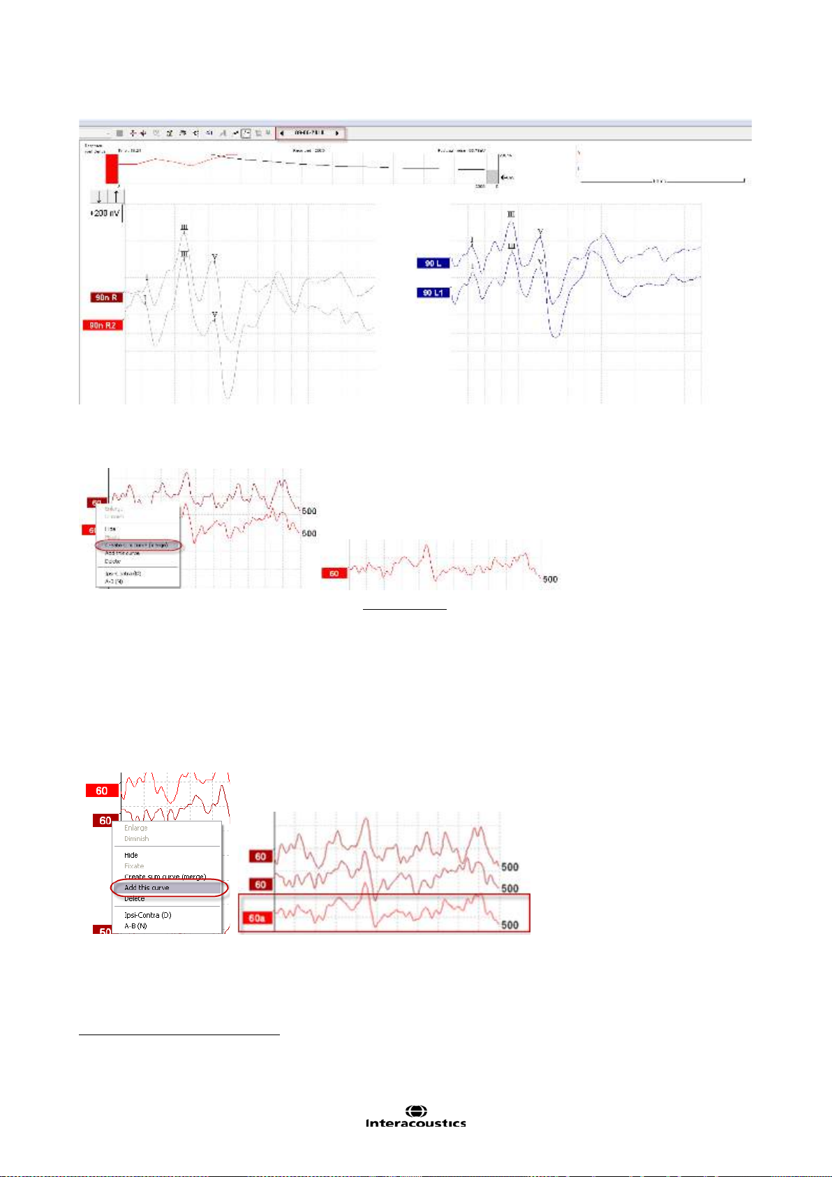
Eclipse Additional Information Page 27
Creating Sum Curve (merge) and Add this curve:
Create sum curve will generate a single curve based on the total average of the individual sweeps of the
two selected curves.
The Sum curve will contain the two merged curves recording sweeps and in this way an improved SNR
reached. The SNR improves by the formula
. .
�
1
is
Instead of merging the curves together to one curve – a third curve can instead be generated.
Add this curve will combine the two selected curve into a third curve based on the total average of the indi-
vidual sweeps of the two selected curves. The added curve will be labelled with an “a” in the handle e.g. 60a
(as shown below). Note New Fmp and Residual noise values are calculated for the combined/merged curve.
However, the graph showing how the Fmp and Residual noise figures change with the number of epochs will
not be available.
1
SNR = Signal to Noise Ratio – the higher the SNR number the better the signal to noise ratio.
Page 38

Eclipse Additional Information Page 28
In order to remove the added curve – use the “Delete” – to delete the curve.
In this way repeated curves can be merged together in order to maximize the reduction of residual
noise if needed.
When using these features the curve must be one of a pair of curves recorded at the same intensity
and of the same ear.
This combined curve may then be split into its two parts again later even after it has been saved in
the database.
Delete (Delete Curve): Right Click while pointing at the handle. In order to remove the added curve press
Delete to delete the curve. Note
Ipsi-Contra (D): This curve will indicate the differenc e bet ween t he ipsi lat eral and c ontr alat era l curv es and is
one way of assessing the noise in general leaving primarily the cochlear microphonic and Wave I visible.
A-B (N): This curve will also indicate the noise in general. However, if the stimulation polarity was alternat-
ing, then the cochlear microphonic will remain and may even sum up to approximately double size for easy
identification.
Export Waveform: Select Export waveform to export the selected waveform as an XML-file. The file is
saved automatically at the destination defined in the Auto Protocol Setup.
This will permanently delete the curve.
Page 39

Eclipse Additional Information Page 29
3.5 Edit tab
Select the Edit tab to enter Edit mode. You may edit a test while an automatic protocol is in progress or after
the test has been finished. For the Edit tab you can then monitor the rejection situation by observing the little
light at the bottom of the screen during a recording. Green indicates no rejection is occurring while yellow or
red indicates higher rejection rates.
3.5.1 Assigning Waveform Markers and Labels
Automatic Procedure
Click on Suggest Waveform Markers.
Now all Waveform Markers, for which Normative Data exists , will be plotted automatically at the most dominant peak within the assigned normative data range. This means that a peak falling outside the normative
data range will have its Waveform marker plotted only as close to the wave peak as the latency template
range allows. This makes it easy to evaluate whether Waveform Markers are within normative range or not.
Sometimes a Waveform Marker may be placed far from the correct position. This happens if the correct position is not the maximum point within the norm data range.
To adjust the position of a Waveform Markers, use the manual procedure explained below.
Manual Waveform Makers and Labels
Waveforms can be marked in three different ways:
1. Click on the marker button (e.g. I, II, III, IV, V) and then click on the curve where you want to place
the marker.
2. Press the marker number (e.g. 1, 2, 3, 4, 5) on the keyboard. Then use the arrow keys, Ctrl + arrow
keys or the mouse to move the cursor to the desired position. Press the enter button or left click with
the mouse to place the marker. Using the Ctrl + arrow keys will move the cursor from peak to peak.
3. Right click on the waveform and select Place maker or Place trough followed by a selection of the
number you want to place.
Page 40

Eclipse Additional Information Page 30
The corresponding ms and μV values will be displayed in the boxes next to the Waveform Markers.
Interlatency values will also be calculated after the relevant markers have been placed.
Manual Marking of Trough
To use the SN10 / trough markers, it must be selected in the General Setup. T r butto ns will app ear for manual positioning of the various troughs including trough V.
.
Signal to noise calculation 3:1
An alternative method to Fmp and residual noise can be used to determine whether a response is present or
not and what the recorded noise is. Place Wave V & Tr waveform markers on the recorded curve.
The Noise is calculated as the deviation between the A&B buffer for each curve in accordance to the Wave
repro line. So if the A&B buffers or wave repro line are moved from their original position a new noise value
is calculated. The Ratio is the Amplitude of Wave V top to SN10 (both markers must be placed manually.
The noise is automatically calculated based on the current Wave Repro line position. Normally this one is not
moved. If it is, a new noise levels for all curves are calculated each time the line is moved. See the below
picture for more guidance.
Page 41

Eclipse Additional Information Page 31
The above markers CR, RA & INC are shown on the Printout together with other relevant parameters such
as the area ratio. Further, note the Ratio in the table indicating 2.9. That is the ratio of interest when comparing peak V and trough V (SN10).
3.5.1.1 Latency times
When Multiple waveform markers on same intensity and side is selected the view of the latency times is
shown on the left of the screen and multiple peaks and troughs can be marked. This screen provides information about the difference between the slow and fast rate in ms for each ear individually, and the difference
between the two ears.
Page 42
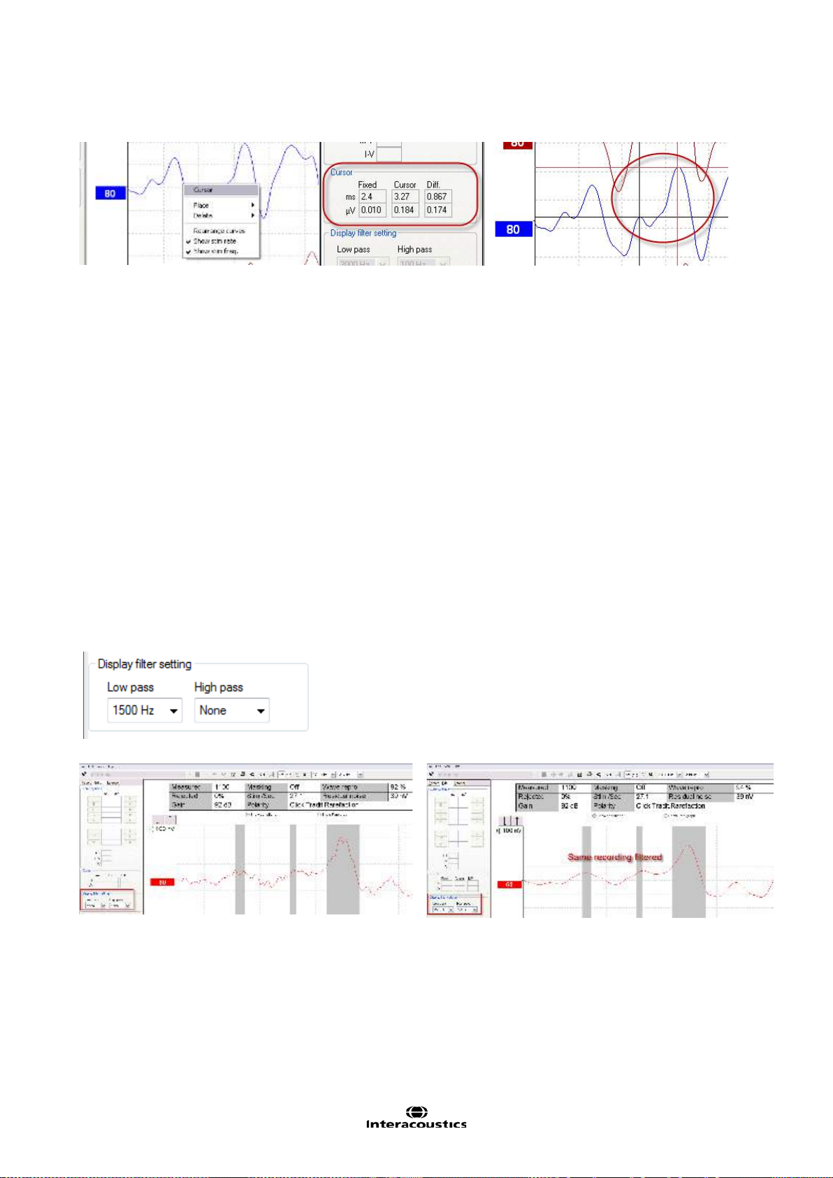
Eclipse Additional Information Page 32
3.5.2 Double Cursor / measuring individual differences
This feature gives you the ability to use two cursors in the Edit Screen. Pointing at the highlighted waveform
(not its handle) and then clicking the right button on your mouse activates the double cursor. Alternatively,
you may select th e curs or by hitt ing the icon View in the upper menu bar.
The first cursor is now frozen at this point. Now move the second cursor to any point on the curve you wis h.
The boxes in the Cursor window will now show the position at which the first cursor was fixed, the present
position of the second cursor and the difference between these two positions. This is a big help if you need
to know the exact difference in amplitude or latency between two points on the curve.
Assign a new position for the fixed cursor by clicking with the normal mouse button. Remove the double cursor by left clicking with the mouse.
3.5.3 Filter settings
You may change the Display filter settings at any time. This will not affect the raw data recording so the
filters can always be disabled again.
This may assist you during the editing function by eliminating unwanted noise from recordings. Using the
Low Pass Filter will typically smooth the curve making it easier to pinpoint the peaks. Using heavy filtering
(e.g. 1000Hz) will often smooth the curve so much that it will be difficult to assign accurate markings to the
peaks. If you are looking only for wave V for fast screening situations, heavy filtering might be applicable.
Conventional Low pass filtering for ABR is 1.5kHz (sometimes up to 3kHz).
The High Pass Filter will reduce the low frequency content of a waveform and thus help in the visual inspection of the curves. Use of very heavy high pass filtering (e.g. 500Hz) will consequently greatly reduce the response amplitude.
Example of curve without filtering Example of curve with filtering
On the Print out the hardware High and Low Pass filters are printed (incl. the high and low pass display filter.
Page 43

Eclipse Additional Information Page 33
3.5.4 Show Conditi on / show Fmp Graph
It is possible to toggle between Show Fmp graph and Show Conditions in the Edit tab. By clicking Show
Conditions the summary of the test settings shown below appear. At the right of the table is the comments
box. Here you can add comments for each curve separately. These comments will be displayed onl y when
the corresponding curve is highlighted. All entered curve comments will be printed out on the Curves Conditions page.
Show Fmp view:
Show condition view:
3.5.5 Latency Template
If latency templates are entered in the System Setup shaded areas indicating the template values will appear
during assignment of the various Waveform Markers.
Note Data for gender and age are taken from the database to provide a correct selection of the corresponding latency template.
Page 44

Eclipse Additional Information Page 34
3.6 Latency tab
Click the tab Latency to enter the Latency window.
Left panel
The two boxes on the left part of the screen provide the latencies of all Waveform Markers assigned to the
curves in this session for right and left ear (see below, left). When selecting InterLatency the information at
the right in the picture below will appear. The view of the inter-latency is split into Right, Left and the difference between R and L for peak inter-latencies as shown below. This information is used in the interpretation
for the ABR.
ABR Latency norms
ABR Latencies are plotted against intensities and a shaded area indicates the latency template data. This
allows for an easy interpretation of latency change relative to the change in stimulus intensity. To assist in
the diagnosis, a grey shaded area of normal responses will be shown providing a latency template has been
entered in the System Setup. Data for gender and age are taken from the database to provide a correct selection of the latency template.
Page 45

Eclipse Additional Information Page 35
An example of a comparison of peak V, III and I. Here the grey area indicates the norm range for entered in
the System Setup. You can add more norms and changes the default ABR normative latency data.
Page 46

Eclipse Additional Information Page 36
3.7 System Setup
3.7.1 Auto Protocols
From the File menu it is possible to enter the System Setup. From here it is possible to modify existing protocols and create ne w protocols.
NOTICE Features not included b y your license will be dimmed or not visible.
Here it is described how you can change and modify your test protocol in general. Please refer to the chapter
describing each test for information about protocols settings for a specific test.
Note. The Auto protocols tab is only available from the current session, and not from historic sessions. Refer
to the condition tab to see what parameters were used for the selected session.
3.7.1.1 Predefined protocol settings
Select the icon New to create a new auto protocol as per all the options in this measurement setup box. Enter the name of your new test in the Name of protocol box. Please note that if no test has been made yet, the
New button is automatically pressed when this dialog box is entered which means that you do not need, and
cannot press New.
Page 47

Eclipse Additional Information Page 37
If you want to edit an existing test sequence, select it from Selected protocol, instead of selecting New. You
have the option to save an edited test with a new protocol name, thus preserving the original protocol.
If you have started the process of creating or editing a test and you want to abort the action press Cancel.
To delete an automated test sequence from the list of predefined tests you must select it in the Selected
protocol window, and then press Delete.
Press OK to save the new test sequence after you have designed it. If you want to abort this setup box without causing any changes what so ever, press Cancel in the lower right corner.
3.7.1.2 Type of measurement
This is where you assign which type of test you want. The tests vary in features available as well as the
length of the recording window: the maximum recording window (epoch) associated with each test type are
as follows:
ECochG: 15ms
ABR-15: 15ms
ABR-30: 30ms
AMLR: 150ms (only if it is included in your license)
ALR: 980ms (only if it is included in your license)
MMN/P300: 980ms (only if it is included in your license)
STS: 45ms recording window with multiple stimuli, each 5 ms apart
(only if it is included in your license)
VEMP: 150ms (only if it is included in your license)
3.7.1.3 Print Wizard
The Print Wizard lets you modify the print out for the selected protocol. Please refer to the section Printing for
a detailed description of the functionally for the Print Wizard.
3.7.1.4 Stimulus properties
Stimulus type
From the drop down four different stimulus options are available. The NB CE-Chirp® LS and CE-C h irp® LS
are optional for the EP15 module and included in the EP25 module. If you have added wavefiles yourself
they will appear from the list (only if the research license is bought).
Page 48

Eclipse Additional Information Page 38
CE-Chirp® (Broadband CE-Chirp®)
In Interacoustics ABR system an additional broad band stimulus (a Chirp), can be chosen if license allows
for it. A chirp stimulus counteracts the temporal dispersion in the normal cochlea and thus presents its lowfrequency energy before its high-frequency energy. The design of the chirp is described in detail by Elberling
et al. (2007a), and has the same power spectrum as a standard click. In the study by Elberling and Don
(2008), it was demonstrated that the chirp ABR is up to 1.5-2.0 times larger than the corresponding click
ABR in normal-hearing subjects. The chirp has also been applied for newborn hearing screening and for this
type of hearing testing it has been demonstrated that the chirp is more efficient than the click.
The practical consequence of this is that responses of a desired signal to noise ratio are obtained in a
shorter test time (or that in a fixed test time, the response will have a higher signal to noise ratio) when a
chirp is used rather than a traditional click.
The above description is the first version of the chirp stimuli from Interacoustics and was named CE-Chirp®.
Elberling et al. (2010) demonstrated that the response amplitude can be further improved by changing the
CE-Chirp model for each stimuli level. This is referred to as the level specific chirp - CE-Chirp® LS.
The level specific stimuli has been further tested in the study Elberling et al. (2012), demonstrating that the
response at higher intensities can be further improved by using the CE-Chirp® LS.
NB CE-Chirp® (Narrow-band CE-Chirp®)
The narrow-band stimuli (octave-band Chirps), can optionally be chosen for frequency specific hearing evaluation. The design and testing of these octave-band chirps is described by Elberling et al. (2007b). These
narrow-band stimuli are also implemented in the Interacoustics ASSR system.
Like the broad band chirp, narrow band chirps hold the promise of a larger response than their traditional
tone burst counterpart whilst offering approximately similar frequency specificity.
The NB CE-Chirps has also been applied for newborn hearing screening and for this type of hearing testing
it has been demonstrated that the NB CE-Chirps are more efficient than the toneburst (Ferm et al. 2013).
The NB CE-Chirp® stimuli has also been changed into level specific octave wide stimuli. To further help and
assist the clinician in the daily testing, the waveform response from the NB CE-Chirps® LS are placed at the
same location as the click response. So for each stimuli level, the entire CE-Chirp® LS stimulus family provides a response located at the same latency timing as it would be for the click response (for normal hearing
subjects).
For further information about the latency norms for CE-Chirp® LS and NB CE-Chirp® LS, please refer the
section about latency norms.
Stimulus rate
Here you assign the stimulus rate per second. For neurological tests 11.1 clicks per second is considered a
reasonable stimulation as this low rate improves the neural synchronization for the waves I-V.
For screening and threshold testing, where the presence of wave V rather than accurate morphology is important, stimulus rates like 45.1 will increase test spe e d.
A stimulus rate of up to 88.8 is available depending on the test type chosen. This rate is particularly appropriate for evaluations of Multiple Sclerosis or other neurological problems (Cochlear Michrophonic test). It is not
possible to have this many stimulations per second and still provide a recording window of 15ms, so the
waveform may be reduced in length, to match very high stimulation rate requirements.
The option for allowing external trigger appears if the minimum stimulus rate is selected.
The recordings below are recording made with different stimuli rates. A compromise between a fast stimuli
rate and not too much smearing of the wave peak morphology is the goal in threshold tests. Please note
there may be large differences of the wave morphology in relation to age and gender.
Page 49

Eclipse Additional Information Page 39
Polarity
Stimulus polarity may be set to Rarefaction, Condensation or Alternating.
Rarefaction and Condensation will each provide slightly different waveforms and either is recommended for
normal ABR. Alternating polarity provides a waveform which is actually a combination of these two waveforms. Such a combination of waveforms may introduce some unwanted distortions to the waveform morphology. The advantage of the alternating stimulation with ABR is that artefacts stemming from electromagnetic radiation from the transducer can be cancelled. Bone conductors can generate very strong artefacts.
An insert phone has hardly any artefact due to its construction.
Tone Burst / Tone pips
The desired frequency of the tone burst is selected here. The following frequencies are available: 250Hz,
500Hz, 750Hz, 1kHz, 1.5kH z, 2kHz, 3k Hz and 4kH z.
Sine Waves (applicable to Burst only)
The desired total number of sine waves cycles of the burst is selected here. Please note, that due to inaccurate use of terms in some early ABR systems, you may see a stimulus be referred to as e.g. a 2-1-2 Blackmann. This is a stimulus with a total of 5 cycles, and this slider should be set at 5.
The longer the stimuli (amount of cycles e.g. 28 cycles) the more frequency specific the stimuli becomes. But
it also means that fewer hair cells are stimulated and smaller responses are expec ted.
On the other hand if the stimulus is narrow, e.g. 2 cycles, the frequency range is much larger and it turns into
a click likely stimuli where most of the hair cells are stimulated. Larger responses are expected, but it also
means we cannot exactly tell which part of the cochlea response occurs from.
E.g. if the patient has a low frequency hearing loss, but some of the hair cells at higher frequencies work,
then the overall response from the narrow stimuli tells us incorrectly that the patient would have a normal
hearing.
Window (applicable to Burst only)
The desired window, which sets the rise and fall parameters of the burst, is selected here. E.g. “Blackmann”
is considered to have good frequency specificity. If you select “Manual” you must set the Rise/Fall and Plateau.
Page 50

Eclipse Additional Information Page 40
Rise/Fall and Plateau (applicable to Burst only)
Here you can design your stimulus manually (if you have selected “Manual” in the “Window” mentioned
above. Rise/Fall sets the number of sine waves it takes before the maximum intensity is reached. The same
number of sine waves will eventually be used in terminating the stimulation. Plateau is the number of sine
waves presented at full intensity. A Rise/Fall of 2 and a Plateau of 1 is popular for ABR testing (= total of 5
sine waves), and is the reference tone burst stimulus described in IEC 60645-3 (2007).
Intensity
Here you select the intensities (between -10dB and 100dB nHL or 20 and 135.5dB peSPL) you want tested
in the automated test sequence. The display of nHL or peSPL depends of your calibration settings.
If you want more than one test performed at the same intensity (for replication purposes) enter the desired
number of tests in the box below.
The intensities selected may be tested in Ascending or Descending order. The S oft Attenuator will assure
that all changes in intensity will happen gradually to allow for a more relaxing experience for the patient.
Also, when initiating a test, the stimulus will gradually increase intensity until the desired int ensity is reached.
Testing of sleeping babies is facilitated by this feature.
If different intensities are needed, the user can enter in the box what intensity they want to see on the
screen. During recording, the user can manually select a new intensity from the user screen.
Stimulus Ear
Select the type of transducer you wish to use as stimulator for the recording.
The instrument is by default calibrated to insert phones (ABR insert or IP30) and optionally DD45s headphones and a B71 Bone conductor. The instrument is only calibrated to the type of transducers supplied with
your instrument.
Please note that all the factory default protocols use the insert headphone. Should you wish to use a different transducer, select the new transducer under Stimulus Ear and save the protocol.
From the drop down “Msk” stands for masking, while “Mnt” in the VEMP protocols stands for monitor.
If Binaural Stim. is selected, the stimulus will be present in both ears. This procedure is used by some hospitals in neonatal screening since evidence of hearing may be found quickly.
Note however that any response might originate for either ear and for individual examination of thresholds at
greater levels it is necessary to test each ear independently.
Masking offset and Masking stimulus
It is possible to apply masking during a measurement for both air conduction and bone conduction measurements.
Masking is available with intensities at a pre-set number of dB above or below any selected test intensity. A
value of -40dB is normally appropriate for air conduction tests. The value should be increased to offset the
effects of an air-bone gap (conductive loss) in the ear to which the masking is applied. Masking is not available if simultaneous stimulation is selected.
White noise (WN) is typically used as a masker for ABR stimuli, the WN level can be considered to be close
to effective masking level. The important exception from this rule of thumb is, that 500Hz TB and 500Hz NB
Page 51

Eclipse Additional Information Page 41
CE-Chirps® LS require slightly louder masking levels of around +10dB. A good reference for getting started
with masking ABR is found on www.hearing.screening.nhs.uk
. The reference refers to a masking calculator
created by Prof. Guy Lightfoot. The masking calculator can be downloaded from the homepage.
If additional masking has been added from the calibration ( as a wa vef ile) of EP they will appear on the list
(only if licensed).
Note as there is no standard for correcting the masking level from SPL into nHL, the masking level are always presented in SPL relative to the stimuli level.
3.7.1.5 Filter properties
Filtering is used to remove unwanted frequencies, and each test protocol holds filter settings for the input
Preamplifier and changing the default settings may remove noise content from the AEP recordings, but may
as well remove some of the response if over filtering is applied. Therefore, it is recommended to follow the
defaults filter settings of the factory protocols to maximize the signal to noise ratio.
On some occasions there might be an electrical noise source within the test ing e nvir onment which 'forces'
you to apply some stricter filtering to get rid of the problems. In such case properly fixing the grounding of the
equipment (and the metal bed) is usually more beneficial than adapting filter settings.
If filtering is applied to smooth the curves, the goal is to make interpretation easier. The Eclipse offers two
different filtering methods 1) Input Amplifier filtering, modified from the System Setup, and 2) Preliminary
Visual display filtering, applied from either the System Setup or the Edit tab.
For the less experienced users, it is recommended to use the display filtering under the Edit tab.
1. Input Amplifier filtering (Filter settings for input amp)
Caution must be taken when setting the hardware filters as it in worst case can result in incorrect recordings. Raw data is
affected.
It is important to pay attention to the filtering as this will influence the recorded AEP response. Here you can
assign the frequency limit above which you want the signal content to be amplified and eventually be present
in your waveform. Contrary to the digital filtering, the filtering you apply here is permanent.
Note These amplifier filters are pre-set and fixed during the recordings and cannot be changed after recording. However if needed it is possible to change the filter for the next recording.
The hardware filters consist of a highpass filter and a lowpass filter.
Page 52

Eclipse Additional Information Page 42
The effect of the Low Pass Filters of the Amplifier
The filter cut off high frequencies chosen by the user. The low pass filter improves the recording conditions
by attenuating unwanted frequency components (noise) and instead allows only the waveform response to
be recorded.
The frequency you choose for the low pass filter is the maximum frequency to record.
The picture below shows the different low pass filters frequency response and steepness for the Eclipse at a
DSP sampling rate of 30kHz.
nd
The low pass filtering is applied by the DSP (digital signal processor) and is a digital FIR filter of the 102
order.
An example of the effect of low pass filtering (LP) is shown below. Note that the hardware LP was changed
prior to each recording under the System Setup, while the display filter was not changed.
Here the low pass filters away unwanted higher frequency components and the waveform response get
cleaner and cleaner.
Page 53

Eclipse Additional Information Page 43
The effect of the High Pass Filter of the Amplifier
The high pass frequency you choose is the frequency above which frequencies are recorded. The number
next to the frequency indicates the filter slope in dB per octav e. At the chosen frequency you will have 3dB
st
attenuation/filtering at the chosen frequency. All AEP high pass filters are analog Butterworth filters of 1
nd
der 6dB/octave or 2
order - 12dB/octave. See below.
or-
2. Preliminary display settings (visual smoothing )
Amplifiers for Evoked Potentials will always have a limited frequency response. This allows signal content
below a certain frequency to be disregarded. Certain tests will have certain desirable frequency limits. This
preliminary filter setting has no consequence for the data recorded, it only affect the visual presentation of
the recorded waveform. This may assist you during the editing function by eliminating unwanted noise from
recordings.
The High Pass Filter will reduce the low frequency content of a waveform (amplitude) - thus helping the visual inspection of the curves. Use of very heavy high pass filtering (e.g. 500Hz) will consequently greatly reduce the response amplitude.
The Low Pass Filter will reduce the high frequency content of a waveform (sharpness) - thus helping the
visual inspection of the curves. Use of very low pass filtering (e.g. 1000Hz) will consequently greatly reduce
the response sharpness (for some less distorted for others with missing details of the waveform). Using the
Low Pass Filter wil
l typically smooth the curve making it easier to pinpoint the peaks. Using heavy filtering
(e.g. 1000Hz) will often smooth the curve so much that it will be difficult to assign accurate markings to the
peaks. If you are looking only for wave V for fast screening situations, heavy filtering might be applicable.
The display filtering applied under Edit tab are all software digital filters, the Low Pass filters (6dB per octave). The High Pass filters are 33rd order filters.
Page 54

Eclipse Additional Information Page 44
Under the Edit tab you can choose display digital filtering of the measurement (which can be done before/during and after the recording).
A default display filter can be set in the System Setup for the individual Auto Protocols. This can if needed be
changed temporary anytime under the Edit tab later.
To see later what hardware filters were used, click a curve and see under the Edit tab on the top or on the
Print out the hardware High and Low Pass filters are printed (see left column) and display filters - right column).
Page 55

Eclipse Additional Information Page 45
Overview of Filtering and Recording
In general the advice is to follow the default parameter of the factory protocols. On some occasions there
might be an electrical noise source within the testing environment which 'forces' you to apply some stricter
filtering to get rid of the problems. In such case properly fixing the grounding of the equipment (and the metal
bed) is usually a more beneficial than adapting filter settings.
If filtering is applied to smooth the curves with the goal to make interpretation easier for the less experienced
users, it is recommended to use the visual filtering under the Edit screen for that purpose (they can be predefined in a protocol).
3.7.1.6 Display properties
From Display properties you can enable and disable the display of rearranged curves and split screen. You
can also set whether the stimulus rate, stimulus frequency, and stimulus polarity must be shown in the end of
each curve. When the parameters are enabled they will appear on the screen during measurement and on
the printout.
Setting the single curve option to On option will default the display screen to Single Curve mode, where only
one curve is displayed at a time. Enabling the Latency Templates option will display available latency template data in edit mode whenever Single Curve display is used.
A preset Volt per division (unit gain) (Volt/Div response curve) can be set. Often 200nV is an appropriate
unit for display under normal ABR testing such as threshold and neurological.
Page 56

Eclipse Additional Information Page 46
The Gain info on raw EEG allows you to change the display of the EEG window; off, in dB, and as a factor
are the options.
3.7.1.7 Recording properties
Stop criteria
Allows you to select the maximum number of accepted stimuli you
need for each test. You can extend the maximum of sweeps on the recording screen.
A typical number of stimuli (sweeps) are
4000. Note the stop criteria should be based on statistical parameters
and a clinical evaluation of the collected curve rather than a defined
number of sweeps.
Response confidence
The Response Confidence drop down lets you change the Response
confidence setting to off, 99%, 97.5% or 95%. Default is 99%, wh i c h
provides the most accurate measure.
The selected criteria can be set as Stop Criteria by ticking the box.
The ABR software calculates the signal-to-noise ratio (SNR) of the averaged ABR waveform. The Response Confidence is based on the
principles described in detail by Elberling and Don (1984 & 2006), and
Don and Elberling (1994 & 1996), and is called Fmp. During the re-
2
cording of the ABR, the actual value of the Fmp (~ SNR
), and a graph
showing how the response confidence develops along with the data
collection (number of sweeps), is presented on the screen.
An Fmp value higher than 3.1 indicates with 99% accuracy that a repeated response is present in the recorded waveform. In this way Fmp
can be used for objective detection of repeated waveforms.
A minimum of 800 sweeps must be recorded before the Fmp value is
used as a stop criteria and ends the test (in order to retrieve sufficient mathematic data).
Residual noise
The Residual Noise Target Line dropdown lets you change the setting for the residual noise target line and
allows you to set the residual noise level as Stop Criteria by ticking the box. When the box is ticked the test
will stop automatically when the set criterion for residual noise is reached.
The residual EEG-noise in the averaged ABR waveform is calculated. The residual noise calculation is
based on the principles described in detail by Elberling and Don (1984 & 2006), and Don and Elberling (1994
& 1996). A Residual noise va lue of 40nV or less indicates that the waveform contains a minimal amount of
noise and the recording can be stopped. Therefore if a response is present it is not due to noise in the recording. If a response is absent with a low residual noise value, it can be concluded that there is no repeated
response in the actual recording, hence averaging can be stopped.
A minimum of 800 sweeps must be recorded before the residual noise value is used as a stop criteria and
ends the test (in order to retrieve sufficient mathematic data).
Page 57

Eclipse Additional Information Page 47
The scale for the residual noise goes from 0nV to 200nV in the combined Fmp & residual noise view. Typically a residual noise level of 40nV is considered by some as a practical noise target for no-response situations. Lower residual noise f igures (ideally 20nV or less) increase the confidence that a response is truly absent rather than being obscured by residual noise.
Fmp range
The Standard Fmp range is calculat ed b y using a 10ms range.
By selecting Manual the Fmp 10 ms range can be modified to the desirable range for a particular test. It is
normal to place the Fmp confidence detector on the timeline where the response is expected, similar to the
older waveform reproducibility.
3.7.1.8 Recording begin and end
If you want the recording to start e.g. 2ms prior to the stimulus onset, select -2ms in the bar. Similarly, you
may delay the onset of data acquisition until maximum 2ms after the stimulus onset. Please note that the
time window of ABR-15 recording is always 15ms for normal ABR, so if the recording is started prior to stimulus onset, then the recording will not quite extend to the 15ms point on the time axis. For threshold testing,
especially with tone bursts at lower frequencies, longer latencies are recorded. Setting the recording to begin
at +2ms has the effect of extending the recording window to 17ms after the stimulus thus aiding in the identification of near-threshold responses.
ABR-30 will provide a 30ms recording window for test routines where 15ms recording window is considered
inappropriate.
3.7.1.9 Rejection
Select the default rejection level for the test protocol. A low rejection e.g. ±20µV level should be used. This
will allow only recordings containing a minimum of amplitude (less noise) to be recorded.
When a rejection level is chosen the gain is also set. When either or both EEG tracings is/are shown with
red, it is indicating full rejection and no recordings are created.
Click Advanced to enter more rejection level settings to specify in which time range normal rejection is applied. By doing this a potential artefact e.g. stimuli, causing the entire sweep to reject, can be avoided.
Simply grab the vertical lines with the mouse and move them along the time axis.
Notice the Rejection disabled areas cannot exceed the Fmp range as this is used for the Fmp and Residual
noise calculation. If you need to adjust the window further, the Fmp range must be moved prior to.
Notice if the grey areas turn red, the recording circuits have been overloaded and to safeguard incorrect recordings all sweeps are rejected. Should you choose to overrule the protection, check the box Disable re-
jection (for eABR only).
Page 58

Eclipse Additional Information Page 48
Fine tuning the rejection level
Simply grab one of the horizontal lines with the mouse and move the rejection level to match an exact value.
The current rejection level is shown to the left on the curve and updated while moving the horizontal lines.
Use the Input Level Display buttons to zoom into the rejection level for more precise rejection level placement. Once done, click OK to save rejection level to the current test protocol.
3.7.1.10 Optimized recording
Bayesian Weighting
Bayesian weighted averaging can optionally be chosen as a method to improve the recording conditions
when the EEG-noise, which depends on the state of arousal or relaxation of the patient, is changing during
the recording of the ABR, and is useful tool to assist the clinician when testing in less than optimal conditions. While giving sweeps with less noise a higher “score”, sweeps with more noise are not given the same
level of importance in the overall recording. Each sweep is analysed and not simply “accepted or unaccepted” (traditional averaging) but given a unique significance based on its level of noise. Bayesian
Weighting can be used in all typical ABR testing situations and will be effective when EEG levels vary during
recording.
Page 59

Eclipse Additional Information Page 49
This method was orig ina lly formulated and tested by Elberling and Walhlgreen (1985). By comparing this
method of weighted averaging to traditional averaging and to different strategies for artifact rejection the superiority of weighted averaging was demonstrated by Don and Elberling (1994).
Measuring without Bayesian Weighting
Note how the residual noise gets worse when the contracted period starts. If the patient would have continued contraction for 10.000 sweeps we would start seeing the noise coming down of course, but it would
never reach the same low level as with Bayesian.
Measuring with Bayesian Weighting
Note how the residual noise still drops in the contracted situation, and never got worse.
Bayesian Weighting does not change the response of a waveform and Bayesian Weighting can be used in
all typical ABR recording situations.
Why use Bayesian?
Optimum use of all data reduces in total the test time
The recordings are more stable, as residual noise will never suddenly rise (and a good waveform deterio-
rate) during recording, even if patient starts to be uneasy.
The difficulty of selecting the optimum rejection level is reduced, as a softer rejection rate can be used
without the noisier sweeps contaminating the more quite sweeps.
When is Bayesian Weighting less Relevant?
If the patient does not have a fluctuating EEG during the session: Bayesian weights noisy sweeps less and
quite sweeps more. In a situation where all sweeps are the same, they will be weighted equally. This is identical to normal averaging. Hence, there is no difference between recordings with and witho ut Bayesian.
Page 60

Eclipse Additional Information Page 50
If a very tough rejection level is set: In this case, all noisy sweeps are simply rejected for both Bayesian and
non-Bayesian recordings. Only the most quite sweeps are accepted, and you have a situation almost similar
to above. With softer rejection criteria (e.g. 80µV) you would benefit from the contributions of the more noisy
sweeps in your averaging thus arriving at your desired residual noise level in less time.
If you run long enough to get a low residual noise level:
If two waveforms each have 40nV residual noise, then they will look equally clean. It does not matter
whether you have used 1.000 or 10.000 sweeps to get there or what type of weighting is used. Weighting will
simply get you there faster if the patient has fluctuating EEG during the session. It should be noted, that two
waveforms each with 40nV residual noise may exhibit minor variations in wave morphology, due to e.g. the
frequency distribution of the residual noise. This may differ with different test situations, and quite patients
tend to provide residual noise with more high frequency content and less low frequency content, which may
look nicer to the eye. So keeping the patient as relaxed as possible is still recommended.
Minimize Interference
When enabled, the system will insert random pauses between the stimuli in the order of a few milliseconds
depending on the rate of stimulation. When adding random stimuli pauses, the recording system will be less
sensitive to periodic electrical interferences as it should minimize the synchronization with the recordings. It
should minimize periodic interference which may, on screen, have a sine wave’s appearance. This approach
is an alternative to the use of a notch filter which carries the disadvantage of phase distortion of the response.
These pauses will not influence the latency times or in any other manner, change the behaviour of ABR responses. Minimize interference is a useful feature to improve recordings made under periodic interferences
such as mains power interference.
3.7.1.11 Wave Reproducibility (Wave repro)
The wave reproducibility monitors the quality of the curve being recorded. Subsequently, when a predefined
quality (Wave repro level) is met, the user can decide to stop the testing and proceed to the next intensity.
The percentage refers to the calculated correlation between the two curves stored in the A buffer and the B
buffer. Even though these two curves are obtained during the same test run, they are actually separately acquired - and therefore independent - data. It is for this reason they may be considered capable of depicting
test reproducibility. Please note that if the polarity of the stimulation is set to alternating, slightly less Wave
reproducibility may be encountered, as the A buffer will hold all the rarefaction data, and the B buffer will hold
all the condensation data resulting in curves which, by nature, will show slightly different characteristics.
The time window you wish to use for the correlation calculation is set by “Wave repro from” and the “Wave
repro to” bars. For neurologic testing a window from 4ms to 8ms will often prove useful. For hearing threshold/screening testing, a slightly later window may be more appropriate.
3.7.1.12 Research availability (only with research licence)
Logging the data for the research module can be enabled and disabled for each protocol from here, and the
destination for the logged data can be changed.
3.7.1.13 Special tests
MMN/P300
This is where you assign how large a percentage of the stimuli for MMN testing shall be of the frequent stimulus type. The rare rate is always 100 minus the frequent rate. Please refer to the description of the Protocol
settings for MMN and the Protocol settings for P300 for more information about the protocols settings for
MMN and P300.
VEMP
This is where you can change the parameters for the VEMP settings. Please refer to the chapter about the
VEMP module for a detailed description of the protocol settings for the VEMP protocols.
Page 61

Eclipse Additional Information Page 51
3.7.2 General Setup
From the General Setup the user can setup and change basic test parameters. The functions not included by
your license will not be visible when connected to Eclipse hardware.
3.7.2.1 External Trigger Output
The unit has an electrical output socket carrying a synchronization signal, by which external stimulation devices may be synchronized to enable ABR recordings.
The trigger pulse can here be set to match the individual requirements of such external stimulator devices.
The scrollbar controls the duration of this brief triggering electrical pulse 5 Volt TTL. Source selects a positive trigger signal and Sink selects a negative trigger signal.
Note Some external stimulation devices do not rely on a synchronization pulse from the ABR unit, but do
themselves send out a synchronization signal. In this case, use the same socket, but disregard this setting,
and set instead the Stimuli per sec. in the Auto Pr oto c ol setup to Ext. Trigger. Please refer to the section
eABR for a detailed description of the Trigger.
3.7.2.2 Auto Protocol Options (Separating ears)
Having the Separating ears ticked off will cause all selected intensities to be tested at one ear before starting to test the other ear. If not selected, the test will follow the selected range intensities in order, testing one
ear at a time before descending or ascending to the next intensity.
The way in which Left and Right recordings are displayed if split screen is not used, is also determined by
this setting.
Page 62

Eclipse Additional Information Page 52
3.7.2.3 Language
There are several languages available for the EP15/25 module. Please ask for and install the separate language CD-ROM. When installed they language settings can be changed from the dropdown.
3.7.2.4 ECochG Area Function
In the setup it can be specified whether the ratio calculation must be based on the Amplitude or the Area.
The number of reference points can be set to 1 or 2. The AP method (Area method) is only available when
the area is selected from the ratio calculation. The setting defines if the area is calculated from AP1 to AP
peak or baseline (BLst) to AP peak.
The cursor amplitude and amplitude ratio functions can be used to calculate the AP and SP amplitudes and
the ratio between the two. These points on the waveform are manually chosen by the user, and the underlying cursor function simply gives the amplitudes and amplitude ratios in those points.
The principle of the user having to manually choose whatever points on the waveforms that is found appropriate remains the same. Not just the amplitudes, but also the areas and area ratios that are between such
manually selected cursor points and the waveform are mathematically calculated and provided as simple
numbers.
This is done to provide a simple mathematical cursor tool to assist those who are interest ed in ca lcul ati ng
such areas.
Please refer to the Quick guide about ECochG to get more information about the use of the area ratio function.
3.7.2.5 Quick stimulus rate
To change quickly between the stimuli rate speed, the Quick Stimulus Rate function can be used. When
enabled the following dropdown will appear on the toolbar during a Neuro Rate Study Examination.
Page 63

Eclipse Additional Information Page 53
3.7.2.6 Special Waveform Markers
In the edit screen, you have additional labels to use for marking points of interest on the waveforms. In contrast to the normal Waveform Markers, these marks may be applied to many waveforms all of the same intensity, as their ms and µV values are not used for the latency/intensity graph. For example, these markers
may be helpful when performing a rate study so that the latencies for a specific wave may be compared at
two different rates for the same intensity.
The Clear Response (CR) user label is intended to indicate that a waveform contains a genuine response.
Local or national criteria may have been defined for this. For example a Signal to Noise ratio above 3:1.
The Response Absent (RA) user label is intended to indicate that a waveform not only contains no obvious
response but also meets local or national criteria for residual noise, thus allowing the tester to be confident
that there is genuinely no response present and therefore that stimulus level is below the hearing threshold.
The Inconclusive (INC) user label is intended to indicate that a waveform is inconclusive (qualifies as neither
CR nor RA). This third option is frequently overlooked but is essential for accurate hearing threshold estimation tests. In general this label will be used to denote waveforms that are of insufficiently good quality to be
allowed to help define the hearing threshold.
Enable Multiple Waveforms Markers if needed, when enabled it is no longer possible to compare curves to
each other and this way calculate inter-latency data.
3.7.2.7 Display Options
Invert Curves on Screen When enabled all curves will be displayed inverted. This is indicated at the vertical
axis with negative values.
Invert ECochG on Screen allows you to invert only the ECochG curves displayed with the wave peaks going downwards.
Auto Single Curve Display Gain will automatically apply additional display gain if the displayed waveform
only has very small excursions. This may allow for an easier identification of peaks.
Page 64

Eclipse Additional Information Page 54
This option carries the potential for the operator to misinterpret the curve. It is important for the operator to note the display scale being used and to estimate the size of any response. Responses that are, in voltage terms, uncharacteristically small or large should be correctly identified as such and not mistaken for genuine responses.
Show EEG too low warning causes a warning to appear below the EEG window when the EEG is too low.
E.g when electrode are short circuited.
Invert VEMP on screen to change the display of the P1 and N1 polarity in accordance to user preference.
Please refer to the VEMP chapter for more information.
Baseline In order to ease the visual evaluation of the curves you can tick off Baseline. Baseline is a horizontal line through the waveform at 0,0µV.
Draw intensity handle at baseline If you find it is a problem that the handle is placed far away from the
curve deactivate the draw intensity handle at baseline, and the handle will follow the curve when you change
the display of the vertical axis.
Show response confidence & residual noise bars will activate the display of the response confidence bar
& residual noise bar (is by default activated).
Show all Contra curves enables the display of all contra curves by default.
Show all A&B curves enables the display of the all A&B curves (rarefaction and condensation) when press-
ing on the Show A&B curve.
Green latency area (normally grey) changes the color of the latency area.
Page 65

Eclipse Additional Information Page 55
Show Standard deviation on EMG graph when testing VEMP, the standard deviation is displayed on the
grap
Leave intensity checkmark on When enabled the intensity checkmark is left on when the intensity is
started. This is beneficial, as the intensity will restart when the running intensity has met the stop criteria defined in the Auto Protocol or when pressing Next intensity from the recording screen.
Waveform order will when enabled shown the order of the collected intensities of each intensity separately
e.g. 80R, 80R1, 80R2 etc.
3.7.2.8 Level measure method
Changes the way to measure the waveform peak amplitudes.
- Peak to baseline, the amplitude from the Jewett mark to the baseline of the entire waveform.
- Peak to trough, enables the Tr (Trough) buttons, mark the peak and bottom peak can be marked manually
and the amplitude is measured.
Trough markers, they must be enabled in the general setup,
Tr buttons will appear for manual positioning of the various trough / SN10 ( V bott o m ) markers. See picture
below.
3.7.2.9 Export Waveform
From this window it is possible to define the destination of exported waveforms when they are exported from
the File menu.
Page 66

Eclipse Additional Information Page 56
3.7.3 Latency Template
Below this tab you are able to enter you own latency template values, relative to patient age and gender.
This Latency Setup permits you to enter latency values which will then be displayed as grey shaded areas
when you assign Waveform Markers on curves.
For these latency values to correspond to the type of patient being tested, latency values for a variety of
combinations of ages and gender must be entered.
Even though the unit may hold examples of latency values when delivered from the factory, it is highly recommended that each clinic enters their own approved latency values, as no international standardized data
exists.
1. Stimulus Here the different types of stimulus frequencies and transducer are selected.
2. Age and Gender As the characteristics of the curves change significantly for babies we have made four
divisions from 0 to 16 months of age. Patients older than 16 months are considered adults. There are also
variations between men and women. For this reason, the gender of the patient can also be added to the Latency Norm.
3. Waveform Markers This feature allows you to add the expected time values at which Waves I, III and V
normally occur. The boxes for “Deviation” define the width of the grey time bar which appears when you start
selecting the Waveform Markers on the curves. After specifying the desired Waveform Markers/Intensities,
hit the “OK” button and then “Yes” for saving the modified norm data.
Data entered here will also specify where the automatic function “Suggest Waveform Markers” will place its
suggested Waveform Markers. If you do not want this function to suggest Waveform Markers at e.g. Wave I
at low intensities, or in other situations where results are often difficult to obtain, do not enter normative data
for these Waveform Markers.
Page 67

Eclipse Additional Information Page 57
Click CE-Chirp® LS NB CE-Chirp® LS
et al. 2012b.
ABR Latency Norms
With the release of EP4.4 the latency norms for Click, CE-Chirp® LS and NB CE-Chirp® LS have been
aligned to make it more straight forward locating the wave V response. The figures below show how response latencies for all three types of stimuli are aligned for the different stimuli levels. Note that age, rates
and filter settings can influence response latencies.
Latency Norms (mean) for the Click, CE-Chirp LS and NB CE-Chirp® LS (500-4 kHz) wave V ABR.
Latency Norms for adults for Click, CE-Chirp® LS, NB CE-Chirp® LS (500-4 kHz) wave V ABR calculated with one
standard deviation (68.2%). The norm values are based on Kristensen & Elberling, 2012; Elberling et al. 2012a, Elberling
Latency norms for CE-Chirp® and NB CE-Ch irp® are als o pres ent in the list if latency norms. The norm sets
are based on Elberling & Don, 2010; Kristensen & Elberling, 2012; Elberling et al, 2012a.
Page 68

Eclipse Additional Information Page 58
Latency norms for the click stimulus for the 3-4 months, 5-8 months and 9-16 month age ranges were provided by Gabriela Ribeiro Ivo Rodrigues & Doris Ruthy Lewis, based on data collected in a published study
(Rodrigues & Lewis, 2014).
3.7.4 Report Templates
You may write various report templates to be used for easy reporting for each session.
Select New, assign a name in the designated area, and now write your standard report template. Remember
that clinic name and patient name etc. is part of the standard header on the printed page. Also realize that
the content of any report template can easily be modified to fit an actual sess ion , with out affecting your original template.
Page 69

Eclipse Additional Information Page 59
3.8 Printing
To print the session, select the print icon in the upper menu bar. The printout will appear according to the
way you have set up your curves with scaling, position etc. The test results will be printed based on the print
template set for the protocol. A default print wizard is set for all protocols. The default can be changed by the
user for each protocol in the System Setup | Print Wizard (see below).
3.8.1 Print options from file menu
There are multiple print options available from the file menu. Print and Print Setup…are functions creates a
physical print.
Page 70

Eclipse Additional Information Page 60
Print anonymous allows you the print a file without patient information, which is beneficial when you want to
share data with others, e.g. colleges or students. The anonymous file still contains the date for test so it is
possible to locate the original file in your database, if you want to do so at a later stage.
To print anonymous to PDF enter the print Setup and select an installed pdf-printer. Exit the printer setup
and press Print anonymous.
Print patient data to PDF creates a PDF-file that is store automatically in the folder defined in the System
Setup | Printer Setup. From here you can also define the naming of the PDF printed file.
It takes approximately 6 seconds to generate a PDF-file, depending of the size of file. While the PDF is generated, the following window will appear on the screen. While creating a PDF it is not possible to use the
module.
Design and preview session lets you modify the Print Wizard for the given session temporarily. From here
it is possible to add additional pages and modify the printout to ensure all the measured data for that particular session is shown correctly on the PDF-print. The file is stored automatically in the folder defined in the
Printer Setup. It is also possible to make temporary changes in the Print Wizard from the Temporary Protocol
Setup.
Page 71

Eclipse Additional Information Page 61
3.8.2 Printer Setup
1. Print view lets you modify the view of the curves (aspect ratio) and latencies on the printout.
2. Native filename formatter By clicking on the Setup native print it is possible to change the destination
of the saved PDF-files. From the dialog it is also possible to modify the view of the patient information separation symbols in the naming of the patient file. The example is shown in the lower part of the dialog based
on the seleced options.
3. Layout of Address fields lets you modify the information provided in the Address field shown in the top
of the printout.
3.8.3 Print Wizar d
When entering the Print Wizard the following window appears. The parts shown in the wizard depends on
the design of the Print Wizard for that particular protocol. The template for each protocol can be modified
from System Setup | Auto Protocols | Print Wizard. When making changes from here the changes are
permanent. Temporary changes can be made from the file menu and from the Temporary Protocol Setup.
The Print Wizard contains of the following menu items:
File | Save automatically saves the Print Wizard template for the current session. Note Save does not save
the file as a PDF, but only safes the print wizard template. To save the file as a PDF select Print patient
data to PDF from the file menu in the main module.
File | Exit closes the Print Wizard window.
Page 72

Eclipse Additional Information Page 62
Elements | Add Quality curves will display the quality curves containing the Fmp and residual noise infor-
mation.
Elements | Add report to add a report field that contains the information you have added in your report.
TM
Elements | Add patient information to show patient information. The information is from OtoAccess
and
changes in the information have to be made from here.
Elements | Add clinic information to show clinical information. The clinical information is from the OtoAc-
TM
cess
database, and changes have to be made from here.
Elements | Add Response Curves the size of the window can be modified. Scaling can be enabled and
disabled in the Printer Setup (see below). When enabled the ratio between the horizontal and vertical axis
stays the same.
Page 73

Eclipse Additional Information Page 63
Elements | Add Latency Curve shows the latency curve information, similar to what is shown in the latency
tab.
Elements | Add Latency Tables provides information about the latencies and inter-latencies.
Elements | Add Condition Tables shows the conditions of the measurement.
Elements | Remove will remove an added element click remove to activate the function and then click on
the element you want to remove.
Page | Add to add a page
Page | Remove to remove a page
The arrows in the toolbar allow you to move to the next or previous page. After adding an element, the size
and display of each element can be modified.
Note it can be a good idea to add curves when setting up a new default print wizard from the Auto Protocols.
Showing the correct number of graphs and marked peaks, latencies and etc., will make it easier to modify
your default print wizard for that particular protoc o l.
Page 74
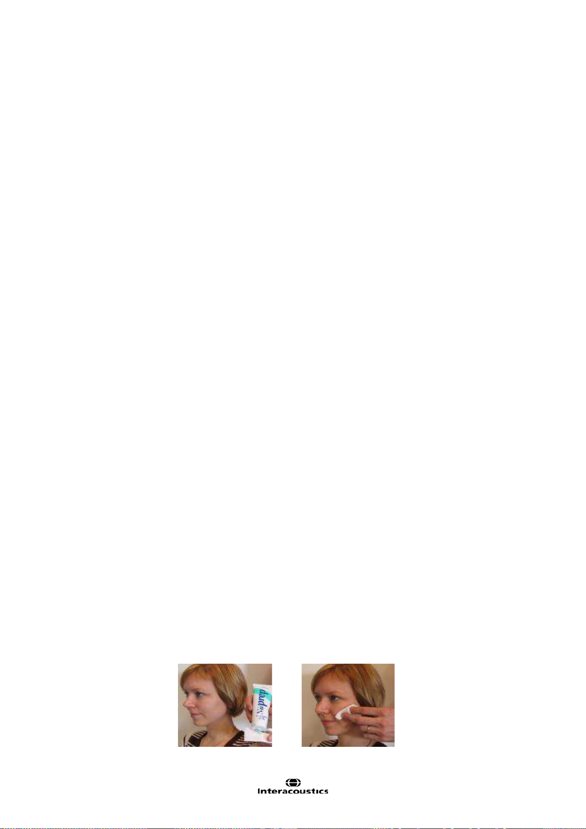
Eclipse Additional Information Page 64
3.9 Preparation Prior to Testing
This description explains how to prepare for testing when perf orming measurements that requires the traditional electrode montage used for threshold examination, neur o lat enc y examination, and etc. For a description of electrode placement that differs from the traditional ABR electrode montage please refer to the Quick
Guide provided with the software installation for the particular test.
3.9.1 Instruction of the patient
The quality of the recordings depends on the state of the patient. If the patient is not physically/mentally relaxed, you will get recordings that are dominated by noise. Therefore, to obtain reliable and valid test results,
it is crucial that the patient is well prepared for the test. Place the patient on a comfortable bed or a comfortable chair. A sitting posture should be avoided due to contracted neck/head muscles. Small children may feel
more comfortable sitting on a parent's or nurse's lap. Show the eartips and electrodes to the patient and then
explain the following:
The aim of the test is to test the function of the auditory nerve.
The tip of the eartips will be inserted into the ear canal.
The electrodes will be placed on your head (depends of selected test).
One or more tones will be heard during the test.
No participation is expected from the patient.
Instruct the patient to relax during testing. A sleeping state is preferred if possible.
Eyes must be closed.
3.9.2 Visual inspection of the ear canal
Check the external ear canal for wax with an otoscope and remove excessive wax to prevent the foam eartip
opening from clogging which will inhibit testing.
3.9.3 Preparation of the Skin
It is very important to clean the skin where the electrodes are to be placed in order to obtain acc ep tab le el ectrode impedance. Be sure not to apply the following procedure to patients for whom it is inappropriate.
Please follow normal clinical procedures for cleanliness and allergy precautions.
The electrode sites must be prepared to assure that the top layer of skin (epidermis) is cleaned and oil is removed. This will ensure low skin impedance for the measurement. For this purpose a large variety of electrode pastes can be purchased. Please note that two different types of electrode pastes exist: One which
rubs off the outer thin layer of the skin and another which is an electrically conductive paste used to adhere
the reusable electrodes. Only the first type can be used for skin preparation (you can feel the abrasive nature
of this type of paste when rubbing it between your fingers). The paste supplied with the unit is this type of
skin preparation paste.
Some clinicians prefer to clean off the paste with alcohol. This will also ensure a very clean area well suited
for the adhesive part of the electrode.
A good and thorough job of rubbing the skin with the paste might turn the skin a little red but will ensure good
impedance. The procedure is displayed below.
Page 75

Eclipse Additional Information Page 65
Neonates generally do not require excessive abrasion. Neonates Alcohol prep pads may be used to prepare
the electrode site. Observe and comply with any local protocol that may limit the agents and techniques used
in preparing electrode sites in neonates.
3.9.4 Placement of Electrodes
Mounting the electrode depends of the type of electrode used. Disposable electr od es are already pregelled, no further gel is needed. Mount the disposable electrode by securing it to the position by firmly pressing the fingertip along the white border around the edge of the electrode pad.
Do not press in the middle of the disposable electrodes when mounting, since this will cause gel to be
pressed out and the adhesive below the white border line will not stick. This will cause the electrode to
loosen from the skin and may cause very high impedances during testing.
For the reusable electrodes apply some conductive electrode gel on all reusable electrodes and mount.
You can use the conductive gel for the reusable electrodes cups after the preparation. Tape can be used to
secure the reusable electrodes in place on the skin. A good tape to use is hospital tape which is a gaze-like
with a good glue/sticky surface. If you carefully pull on the electrode some seconds after application, the
electrode should remain tightly adhered to the skin.
Note Mounting the electrodes correctly is crucial for a good measurement. When mounted correctly it should
be possible to achieve impedance in the range 0.5-1kOhm.
Place an electrode on each mastoid or earlobe (blue electrode lead on left side, red on right side) one at the
vertex or hair-line (white electrode lead) and the ground connection (black) can be placed on the low forehead or side of the forehead. The placement of the ground electrode is not very critical, though in general it
should not be placed within about 3cm of any other electrode. It is a good idea to attach the cable and the
electrodes before placing them on the head to avoid unnecessary pressure on the electrodes while they are
place on the patient.
Note, that all four/three electrodes should be positioned (EPA4/EPA3). In other words all electrode sockets
must be occupied.
The disposable electrodes supplied with the unit are single use types, which are already prepared with electrically conductive paste. No additional electrode gel/paste is needed.
Note Positioning of the white electrode at the true vertex will provide ABR and cortical response waveforms
with higher wave amplitudes.
If the hair-line montage is used, move the electrode as close to the hair-line as possible for best results. In
general the lower the active electrode is positioned the smaller the response.
Generally the system can be used to record any potentials generated by muscles, nerves etc. (including research on animals). However, pay attention to the amplitude and rate of the signal to record.
Place an electrode on each mastoid (or earlobe), one at vertex (or hair-line) and one on the cheek or low
forehead. Connect all four electrode leads.
After having attached the electrodes to the patient, it is crucial to check if the skin impedance is acceptable.
For best results, impedance at each electrode site should be as low as possible; preferably 3kΩ or less and
best if they are balanced.
Page 76

Eclipse Additional Information Page 66
trode.
If a socket is left open or a cable not connected to the patient via an electrode, rejection will occur and testing will not be possible. Both the ipsilateral and contralateral EEG is evaluated to determine rejection.
3.10 Impedance Check
Press the Imp. button
and turn the dial fully
clockwise.
Low and balanced electrode impedances are typically more efficient in reducing interference.
If the impedance of one or more electrodes is too high, consider rechecking the bond between the skin and
electrode. If this does not help you may need to remove the electrode and repeat the skin preparation procedure using a new electrode.
Return to recording mode by pressing down the IMP button again. All Preamplifier LED turns off.
Turn the dial slowly
counter clockwise.
The LED for each
electrode will change
from red to green as
the impedance is
found for each elec-
Press the Imp. button
to exit the impedance
mode before testing.
3.10.1 Insertion of eartips
The final element before starting the test it to insert the eartips. Alternatively headphones or a bone conductor can be used as transducer.
1. Make sure that the end of the black tube is not covered by the yellow foam when you roll the tip into
the smallest diameter possible.
2. Insert the tip well into the ear canal. The correct insertion depth into the ear canal is obtained when
the rear edge of the tip is 2-3 mm inside the entrance of the ear canal.
3. Secure the tip in the ear canal until foam expands.
Use a new pair of ear tips for the next patient.
Page 77

Eclipse Additional Information Page 67
3.10.2 Placement of bone conductor
When testing with the bone-conductor, stimulus artifacts will be present at intensities near maximum output.
Reduce the artifact by placing the electrode on the front of the earlobe instead of mastoid position. Placing
the bone conductor too close to the electrode causes artifact and more noise in the recording. A good rule of
thumb is to keep the electrode and bone-conductor minimum 1 cm apart from each other.
2
Mastoid is preferred as it is 30dB more sensitive than forehead
. Consider bone conductor location before
applying electrodes. Place Mastoid electrode below bone conductor for the largest ABR response but not on
the neck muscle.
BC placement on the temporal bone slightly posterior to the upper part of the pinna gave similar ASSR
thresholds to a placement on the lower mastoid.
Most bone conductor headbands are too big to fit the head of an infant. Hand-holding the bone conductor
can be used for the mastoid position. Firmly hold the bone-conductor with a finger on the infants head.
Experiments on an artificial mastoid showed differences of less than 1dB in stimulus level between finger
pressure and standard force of 5N.
Do not use two fingers as this reduces the stimuli level. Make sure not to touch the pinna with the bone-conductor or the surface electrode.
Start testing at moderate level (e.g., 30dB nHL). A higher intensity might wake up the sleeping infant.
3
3.11 ABR Masking
As in Pure Tone Audiometry, problems occur with con duc ti ve hear ing loss es , where cross-masking can occur.
Differences between ipsi and contralateral waveforms are used to identify the side of the response
Two approaches to detect the hearing ear.:
(a) Presence or absence of wave I (CE-Chirps® helps to give larger amplitudes also wave I which is an indication of the stimulated ipsi ear is responding).
(b) Asymmetry between ipsi and contralateral recordings, earlier latency and larger amplitude on the side
generating the response.
If a contra response is found, masking should be applied.
An ABR threshold can be masked to ensure that the threshold level is not overheard. The easiest way to apply masking during a measurement is to stop the measurement or wait until the current recording is complete.
Masking on new-borns and children should be applied when the interaural hearing difference between right
and left ear exceeds:
• Insert phones = 60-70dB nH L
• Headphones = 40dB nHL
• Bone = 15dB nHL
Masking bone, studies indicate an inter-aural attenuation of 20 to 30dB, probably no need to mask at or below 15dBeHL.
If response seen at 15dBeHL then it must be from the ipsilateral ear. If right ear and left ear thresholds are
no more than 15dB apart (10dB at lower frequencies) then no need to mask.
4
2
http://hearing.screening.nhs.uk/
3
Small, Hatton & Stapells (2007)
4
http://hearing.screening.nhs.uk/
Page 78

Eclipse Additional Information Page 68
3.12 ABR Threshold Determination
For a child not able to co-operate in traditional audiometric tests, ABR is a popular and effective way to evaluate hearing threshold.
This is done by testing at different stimulation levels and evaluating the resulting waveforms for responses
related to the sound stimulation. Often a descending stimulation protocol will be used for each ear independently. Masking may be applied if a large unilateral hearing loss is found or when testing by bone conduction.
It is possible to change from the normal broad frequency range Click stimulus to the more frequency specific
tone Burst stimulation, to obtain a closer resemblance with traditional audiogram findings. Such testing may
reveal responses down into the 10-0dBnHL region for normally hearing babies, depending on many factors
like degree of relaxation, the number of sweeps done and the electrode positioning.
The ABR allows the use of the following stimuli for threshold determination:
NB CE-Chirp® LS & CE-Chirp® LS or NB CE-Chirp® & CE-Chirp®
Click
Tone burst (TB)
3.12.1 Protocol Settings for Threshold Determination
There is variety of test protocols available for Threshold Determination. By default the Threshold Protocols
parameters are the same. The default threshold protocols are optimized for children.
Page 79

Eclipse Additional Information Page 69
Type of measurement: ABR-30
Stimulus Ear: Insert phone
Filter properties: LP: 1.5 kHz/12dB/oct
HP: 33 Hz/6dB/oct
Stop criteria: Residual noise ≤ 40nV
Recording: Optimize recording Bayesian weighting
Rejection level ± 40µV
Display: Split Screen enabled
Multiple Waveform Markers disabled
There are protocol differences on:
Stimulus properties: Stimulus type (CE-Chirp® LS, NB CE-Chirp® LS, Click and Tone Burst)
Stimuli rate (45.1, 35.1)
Stop criteria: Fmp range is set individually for each threshold frequency.
Recording: Set individually for each threshold frequency.
Display: Choose to show Polarity
Wave reproducibility: Changes depending of the selected stimulus and frequency.
Note All default parameters can be changed if needed.
For information about the test procedure please refer to the relevant quick guide.
3.12.2 ABR Threshold Results
This is an example for a Threshold determination using CE-Chirp LS for the left ear. In the given case the
threshold is 10 dB nHL.
Page 80

Eclipse Additional Information Page 70
3.12.3 Protocol Settings for Bone Conduction ABR
The EP15/25 contains the default bone conducti on pr otoc ols: Bone Conduction CE-Chirp LS, Bone Conduction 2 kHz TB, Bone Conduction 2 kHz NB CE-Chirp LS, and Bone Conduction Click.
One of the main test parameters of interest when performing a BC ABR is the Stimulus ear. Here the type of
transducer is indicated for masking, and it is possible to adjust the masking level from the dropdown. This
function is also available from the Temporary Protocol Setup.
Page 81

Eclipse Additional Information Page 71
3.13 Neuro Latency Examination
If there is a tumour affecting the hearing nerve, the transmission time is prolonged. Since the transmission
time is fairly stable between individuals of the same age group, it is common to compare the latency of the
response against a set of ABR normative data. This will reveal if the patient has normal nerve transmission
times or should be referred for more extensive testing due to the presence of transmission times longer than
expected. There will, of course, be some variance between individuals when determining normative latency
times. A common test is to compare left ear’s latency times to right ear’s latency times, as they should match
very accurately. When doing this comparison, remember that a unilateral hearing loss may also cause a
longer latency time at the impaired side. This is because the stimulus is perceived with lower effective intensity and lower intensity by itself causes a longer latency.
3.13.1 Protocol Settings for Neuro Latency Examination
The Latency protocol is used for comparison of the latencies between left and right ear.
The Latency protocol is using a slower rate (slower rates can also be used) – and high intensity stimuli. This
should provide clear ide ntif i abl e waves peaks.
For information about the test procedure please refer to the relevant quick guide.
Page 82

Eclipse Additional Information Page 72
3.14 Neuro Rate Study Examination
The preprogrammed Rate Study test is designed to evaluate the integrity of the auditory nerve. The purpose
of the test is to look for retrocochlear lesions abnormalities along the auditory pathway. Changes in response
latency between fast stimulation rates and slow stimulation rates are recorded and compared. The Eclipse
offers both slow and fast markers and performs the calculation between the inter-peak Wave V latencies (between Left and Right) as well as the intra-peak latency shift change from slow to fast rate.
3.14.1 Protocol Settings for Neuro Rate Study Examination
The Rate Study protocol is used for comparison of the latencies between fast and slow stimuli rates.
To change quickly between the stimuli rate speed – the quick access stim. rate function can be us ed - these
can be manually changed if needed under the General Setup.
For information about the test procedure please refer to the relevant quick guide.
Page 83

Eclipse Additional Information Page 73
3.15 eABR – Trigger Enabled (if included in your license)
The Electrical Auditory Brainstem Response (eABR) is a measurement of the ABR using an electrical stimulus. The purpose of the test is to determine if the auditory nerve responds as expected to electrical stimulation. The stimulus to elicit the response comes from an external cochlear implant stimulator not supplied with
the EP25 system. The cochlear implant system also determines the stimulus and level. The test is used to
evaluate electrical threshold while stimulating with a Cochlear Implant, the result is typically used to ensure
brainstem activity and determine how to set the cochlear implant levels.
3.15.1 Protocol Settings for eABR
A special auto protocol setup of the EP25 system has been made that will set the measuring range typically
used for this type of measurements as shown below.
eABR Protocol
External Trigger: Active – Tr iggered b y Cochlear implant system
Transducer: Not used
Stimulus: Elicited by Cochlear implant system
Masking offset: Not used
Repetition Rate: Controlled by Cochlear implant Stimulus System
Polarity: Not used
Filters: 1–5kHz or 3kHz
Time base: 0-15ms or 0-30ms
Disable rejection: Enabled
Page 84

Eclipse Additional Information Page 74
3.15.2 Using the Eclipse Trigger
To describe the Eclipse trigger an example of the Eclipse connected to a cochlear implant stimulator is used.
The cochlear implant stimulator is provided by the manufacturer of the cochlear implant.
Left: The trigger socket on the back of the Eclipse. Center and left: The PPS box from Cochlear Nucleus and
it setting.
The trigger signal to synchronize the EP25 and the Cochlear Implant Stimulator may work in one of two
ways:
1. A signal is sent from the EP25 software on the Eclipse to the Cochlear Implant Stimulator
2. A signal is sent from the Cochlear Implant Stimulator to the Eclipse hardware.
Sending the trigger (synchronization) signal from EPx5 software:
Under the EPx5 General Setup you must select the type of trigger signal your Cochlear Implant Stimulator
device needs (Source or Sink):
The trigger signal is a 5 Volt square wave standard trigger signal
which is either positive (Source) or negative (Sink). The duration of
the trigger signal can be set to meet the needs of the Cochlear Implant Stimulator device. You may find such specifications by referring to the technical specifications supplied by the manufacturer of
the device, or simply by trial and error.
The onset of the trigger signal starts at 0ms on the recording scale, however the duration of the trigger signal
can be changed to work in accordance with manufacturer specifications.
Cochlear Implant Stimulator sendi ng the trigger signal:
Under the EPx5 Auto Protocols tab, the eABR protocol setting for Stimuli per
sec, must be set to Ext. Trigger (move the slider to the far right) in order to enable the “External Trigger”. This allows the EPx5 to record a measurement every
time a 5 Volt Source signal (duration >10ms) is sent from the Cochlear Implant
Stimulator. The stimulus rate from the Cochlear Implant Stimulator or other external device, must not exceed 50 per second in order to allow sufficient recording and processing time.
Ensure that the trigger signal is actually being sent from the Cochlear Implant
Stimulator to the EPx5 software. It may need to be manually enabled in the
software provided by the manufacturer of the CI or ABI.
Page 85

Eclipse Additional Information Page 75
Trigger Cable
Connection to the Eclipse is via a standard 6.3mm stereo Jack. The “Trigger In” signal is on the tip of the
jack.
The “Trigger Out” signal is a stereo jack with the signal present on the “middle ring”. Ensure that the trigger
cable used is a stereo jack. A mono jack will not work.
Ensure that the trigger signal is actually being sent from the Cochlear Implant Stimulator to the EPx5 software. The trigger signal may not be enabled when the speech processor box/PPS communicates with the
Cochlear Implant. It can be enabled under the software on the Cochlear Implant computer.
Trigger Cables
The following two cables sold by Interacoustics are compatible for use with Cochlear implant devices. The
cables are available in either 1.5m (Part #: 8004222) or 5m (Part #: 8004236).
An eABR trigger kit can also be ordered number 8105928. This includes the below two cables and the EPA3
cable collector.
8105924 cable for AB/MedEl/Neurolec/Oticon Medical
8004222 cable for Cochlear Nucleus
1. Connect the trigger output of the Cochlear Implant computer to the trigger input of the Eclipse
2. Start up both the Eclipse and CI system .
3. Select the eABR auto protocol under the EP25 list.
4. Do a trial test (no patient connected) if this is first time to perform the eABR – to make sure the two
system are communicating as expected.
Example: Set the CI system to generate a stimuli and a trigger signal. The EPx5 system must make a
recording when receiving the trigger signal. The preamplifier electrodes can be short-circuited oth erwise it will report rejection.
5. Connect the patient
6. Set up the cochlear implant computer and follow the eABR instructions as specified by the cochlear
implant manufacturer.
7. Select the electrode band to stimulate on the CI-system
8. Click on the Start button to start. The Eclipse EP25 system will wait for the triggers to start acquisition.
For information about the test procedure please refer to the relevant quick guide.
Page 86

Eclipse Additional Information Page 76
3.16 ECochG (Electrochochleargraphy) (if included in your license)
Electrocochleography (ECochG) is a measure of the electrical potentials of the cochlea, which appear within
the first few milliseconds of the response. Typically, the measurement is characterized by the stimulus onset
(baseline), the response of the cochlea to the stimulus (summating potential - SP) and response to the synchronous firing of nerve fibers (action potential - AP). The AP is also known as Wave I. The cochlear microphonic (CM) is also part of the ECochG, but has its own protocol because the settings for measuring CM is
different from the parameters needed to highlight AP and SP.
To have as strong a signal as possible, it is recommended to record from a point as close to the site of generation as possible.
3.16.1 Protocol Settings for ECochG
It is recommend to use insert phones for the measurement to be able to make a clamped reference measure. The time window is set to within the first few milliseconds as they are of interest.
For information about the test procedure please refer to the relevant quick guide.
Page 87

Eclipse Additional Information Page 77
3.17 Cochlear Microphonic (CM) (if included in your license)
The presence of CM and absence or abnormal ABR is used in the diagnosis of auditory neuropathy spectrum disorder (ANSD). When a click ABR is not present or abnormal performing an CM test should be considered as an important part of the ANSD diagnosing to examine if the response from the OHCs is present
(normal or abnormal).
To have as strong a signal as possib le, it is recommended to record from a point as close to the site of generation as possible.
3.17.1 Protocol settings for CM
The protocol makes used of a fast stimulus rate, and is set with an alternating stimulus. The parameter of
interest is rarefaction and condensation with is enabled by pressing
(condensation (+) and rarefac-
tion (-)) prior to starting the test. Alternatively, you can enter the Temporary Setup to change the
polarity if you want to measure one curve as condensation and one curve as rar efaction.
It is recommend to use insert phones for the measurement to be able to make a clamped reference measure. The time window is set within the first few milliseconds as they are of interest.
For information about the test procedure please refer to the relevant quick guide.
Page 88

Eclipse Additional Information Page 78
3.18 AMLR (if included in your license)
AMLR has the potential to offer a more complete picture of the status of the auditory system and can be
used to help determine the degree of hearing loss. The most common neurological use of the AMLR is for
the assessment of the functional integrity of the auditory pathway above the level of the brainstem in cases
with suspected lesions and for the assessment of nonorganic hearing loss.
3.18.1 Protocol settings for AMLR
The test parameters are set to highlight the subcortical regions (Na) and Pa components occur r ing aroun d
18-80ms.
An AMLR should be measured using traditional ABR stimuli, such as Toneburst 250Hz-4kHz, stimuli
from the CE-Chirp® stimulus family and custom wave files at an moderate intensity level.
For neuro diagnosis a moderate stimuli intensity below 70dB nHL is appropriate.
For estimation of threshold response amplitude follows the stimuli level as for traditional ABR thresh-
old testing – e.g. starting at a level of 45dB nHL and determine to step up or below 20dB nHL to
threshold.
A slower rate is indicated for younger children or for patients with cortical pathology. Normal rate for
adults is below 7.1 stimuli per second.
Stimuli rates as low as 1 per second or 0.5 per second are required to consistently record the Pb
component.
For information about the test procedure please refer to the relevant quick guide.
Page 89

Eclipse Additional Information Page 79
3.19 ALR (if included in your license)
These tests are concerned with revealing responses at cortical levels, where well documented responses
can be found in the 100-500ms range. A time window of up to 980ms provides possibilities here.
The N1-P2 cortical response may be used for threshold evaluation in adults and older children.
3.19.1 Protocol settings for ALR
EP25 comes with the default ALR protocols ALR 2kHz TB and ALR Click.
The protocol settings for ALR depend on the parameters of interest. A good guideline to modify the test parameters in your ALR protocol can be found on www.corticalera.com
MMN.
For information about the test procedure please refer to the relevant quick guide.
. A specific protocol exists for P300 and
Page 90

Eclipse Additional Information Page 80
3.20 P300 (if included in your license)
P300 and MMN are popular ALLR tests. Both of them rely on their electrical responses of the patient’s attention to the stimuli. Two different stimuli like 1kHz and 2kHz are presented randomly but with different relative
likelihood – one is frequent and the other rare (typically only 20% of the time).The patient is asked to count
all the rare stimuli and disregard the frequent ones. Two independent curves are then recorded; one for each
type of stimulus. A normal response will be a deflection around 300ms from stimulus onset (P300) on the
curve recorded for the rare stimulus.
3.20.1 Protocol settings for P300 (if included in your license)
A test designed to retrieve the P300 response phenomenon, which is present approximately 300ms after
stimulus onset. It occurs as a response to a stimulus, which differs from a stimulus to which the patient is accustomed. The rate between the accustomed stimulus and the rare stimulus is approximately 80/20. The test
setup must specify both the frequent stimulus and the rare stimulus, which can be adjusted from the Protocol
Setup in the field highlighted above.
For information about the test procedure please refer to the relevant quick guide.
Page 91

Eclipse Additional Information Page 81
3.21 MMN (if included in your license)
Mismatch Negativity Test (MMN) is designed to retrieve the MMN response phenomenon, which is present
approximately 250ms after stimulus onset. The MMN is present on a calculated differential curve found by
subtracting two waveforms where one is recorded with a frequently appearing sound stimulus and another
recorded with a rare appearing different sound stimulus. Unlike the P300 patient does NOT need to pay attention to the stimuli.
3.21.1 Protocol settings for MMN
The MMN Frequent rate is typically set to 80% frequent and 20% rare. The protocol for MMN differs slightly
from the P300 protocol with the time window being the main difference. The test setup must specify both the
frequent stimulus and the rare stimulus, which can be adjusted from the Protocol Setup in the field highlighted above.
For information about the test procedure please refer to the relevant quick guide.
Page 92

Eclipse Additional Information Page 82
3.22 Loop Back
The loopback test is described in the chapter “Ensuring the Eclipse is working properly”. Please refer to
the chapter for information about the test procedure.
Page 93
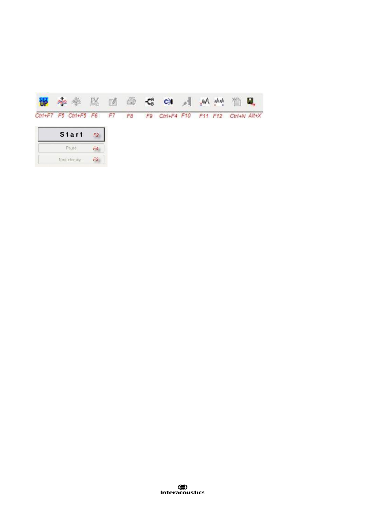
Eclipse Additional Information Page 83
3.23 EP 15/EP25 PC shortcuts
Many of the functions carried out by dragging and clicking with the mouse can be accessed also from the
keyboard. Once you get to know these functions, you may find them faster and easier than using the mouse.
Icon descriptions and keyboard shortcuts can be viewed by hovering your mouse over the icon of interest.
Other shortcuts
Crlt+F10 All Contra are displayed
Shift+F9 All A&B buffers are displayed
Tabs
Use Alt+V to open the View tab while you hold down the Alt key, select the underscored letter to make the
desired selection in the menu. This procedure works for all tabs which hold an underscored letter.
Recording Screen
Change waveform size with the arrow keys.
Edit screen
You may select the Wave I through Wave V buttons, simply by selecting the corresponding numbers 1
through 5 on the keyboard.
You may move the marker with the arrow keys on the keyboard. If you use Crtl+Arrow key then the marker
will jump from peak to peak for easy selection of correct position. Place the marker mark by hitting Enter on
the keyboard.
Above procedure is also an easy way to adjust Waveform Markers which are positioned incorrectly, e.g. by
the Suggest Waveform Marker function.
General size of the waveforms is controlled with the arrow keys.
Page 94

Eclipse Additional Information Page 84
Page 95
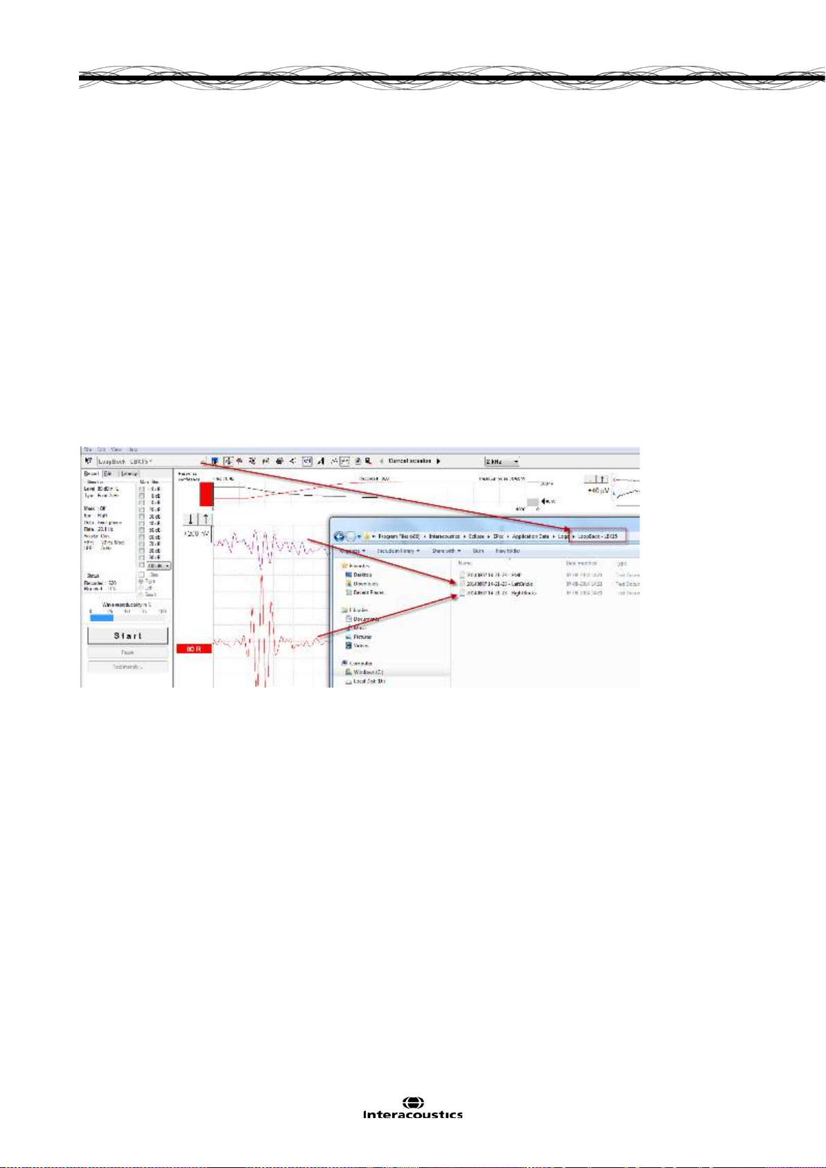
Eclipse Additional Information Page 85
4 Research Module
The research module license enables options to export averaged curves. It can also be used to log each
sweep so the entire recording can be “replayed”. The exported data can be analyses further in e.g. Excel
and Matlab programs. Please refer to the instruction for use, chapter Research Module for an introduction of
the research module. This chapter describes parameters and functions of the Research module into more
details.
4.1 Logging data (while recording)
Logging of data results in 3 txt files being generated and placed in the specified log folder. Below is an example recorded using the test protocol LoopBack LBK15.
A folder with the protocol name is automatically created where the logged files are saved - In this case below
3 files for one recording is generated and saved.
1. First is the Fmp/ Residual noise curve.
2. Second the contra curve (called LeftBricks .tx t) .
3. Third the 80 dB nHL 2kHz LBK response from the right side. (called RightBricks.txt).
Depending on if the data are logged or they are exported, the following parameters are to be considered.
Logging the recording.
The logged data consist of blocks each holding 10 sweeps.
So e.g. in excel you see a total list of row of 60 blocks, the total number of sweeps is 600.
The logged data are filtered by the High pass Hardware filter and the antialiasing filter at LP 5kHz.
Furthermore is the Low Pass HW applied to each of the logged data.
The visual display filters and Bayesian are not included to the logged data.
Page 96

Eclipse Additional Information Page 86
4.2 Exporting the single curve
To export one curve of interest, right click at the intensity handle to export this averaged waveform.
The exported curve is an XML-file located in the specified Export Waveform folder.
4.3 Exporting the whole session
Click Menu-File and Export session to export the full session of the averaged data seen on screen.
Below an example of six curves that has been exported to an XML-file and saved in the folder “Exported
Waveforms”.
When exporting a waveform or entire session:
The exported average waveform is including Bayesian and the two HW filters.
The visual display filters are not included.
Page 97

Eclipse Additional Information Page 87
Opening the above XML in Excel, Internet Explorer, XML viewer or Matlab, you will see the same structure
as described when exporting one waveform per time.
The six curves (3 right and 3 left) are listed in the spreadsheet when scrolling down the list.
4.4 Exporting waveform when offline
The recorded data is available for export when the Eclipse is not connected, but only if the recordings are
made on an Eclipse with license for the research module function.
4.5 Exporting data from another laptop
If the recording are made on an Eclipse with the Research license (export function is available) – the recorded data is indicated research mode is possible (both import wavefiles, export waveform, export whole
session).
4.6 Exporting other data
If the laptop is connected to an Eclipse with the Research license, the averaged recorded data can be exported.
Page 98

Eclipse Additional Information Page 88
Maximum voltage analog to
digital converter
1.6V constant number
Digital resolution
16 bits constant number, means it can represent the data with ± 32768.
Sampling rates
Typically 30.000Hz but depends on measurement type.
Number of samples per curve
Typically 467, see string “NumberOfSamples”
Number of sweeps
See string “NumberOfMeasurements”
Recording time
See string “PrestimulusSamples” and “ScreenStartPos” and “ScreenEnd-
Pos”
WAV file for stimuli
The WAV files format must be 16bit using a sampling rate of 30kHz.
The maximum length of the WAV stimuli is 1.09227 sec.
Gain
Often set to 92dB, see string “Gain”
Preamplifier output
12VAC
Stimuli rate
“StimulusRate”,
4.7 Technical details of the research module
For visualization of the recorded data there are important parameters to know and understand in order to
reestablish the EPx5 recordings in e.g. Excel and Matlab.
An overview of the most used parameters needed for extracting data from the research module are
See string “SampleRate”
ABR15 sampling rate is 30kHz. Recording time 15ms.
ABR30 sampling rate is 15kHz, reduced a factor 2. Recording time 30ms.
VEMP sampling rate is 3kHz, reduced a factor 10. Recording time
150ms.
ALR sampling rate is 500Hz, reduced a factor 60. Recording time 900ms
Only 450 are displayed as 17 points are used for the filter algorithm.
Please be informed when logging data that the exported data consist of
blocks, each holding 10 sweeps. E.g. 600 sweeps have been conducted,
you will see 60 logged data in the string.
For an exported session you will have one “block” which is the average of
all the sweeps.
Number of measurements
Stimuli type
Frequency
Transducer
The sampling rate of the Eclipse is 30 kHz with an Analog to Digital resolution of 16 bits.
The numbers of dots per trace is specified by the variable “NumberOfSamples” in the xml file, which is typically 467 dots displayed per trace.
If a fast stimuli rate has been used for the test, the number of dots per trace may be less, this means in other
words that the curve is getting shorter to maintain the high stimuli rate.
“NumberOfMeasurements”,
“StimuliType”,
“Frequency”
“Transducer”
Page 99

Eclipse Additional Information Page 89
4.8 Import of XML-file in external program
Use e.g. Excel, Matlab, Notepad ++ (freeware), Microsoft notepad or Internet explorer to open the XML-file.
To open the file in Excel, select how you want to open the file in the dialog below.
4.8.1 Import in Excel
Users then can pull the data into an Excel Spreadsheet using the function under ‘Data ‘ tab. ‘From Other
sources’>’From XML Data Import’
Upon clicking ‘Open’, the data will automatically populate the Excel Spreadsheet with appropriate headings.
Alternatively, drag the XML file into the excel sheet.
When selecting As an XML table the following the data will be displayed in columns as shown below. The
headings (the first row) in Excel show the parameter names. The two pictures of data illustrate the A & B
buffer. The last 4 columns in the Excel sheet, using XML table option, are Ipsi A & Ipsi B buffer, and contra A
and Contra B curve (called IPSI_A_Raw, IPSI_B_Raw, Contra_A_Raw and Contra_B_Raw in html viewer).
The contra curve is also made of 2 buffers (A & B). This display option is not available in the the EPx5 software, where only the averaged contra curve is displayed.
Page 100

Eclipse Additional Information Page 90
If opening from Excel and choosing the format As a read-only table workbook, the data sheet is rearranged and renamed into IPSI & Contra. See picture below with the red square.
Here an example of a single block of B-Buffer data displayed as a graph in Excel. The loopback 2kHz stimuli
is presented in the beginning of the curve. The entire curve is overlaid with a 50Hz interference stimuli.
 Loading...